Master Thesis

Models for the Steiner Tree PackingProblem

Michael Sausen

Master Thesis DKE 13-20

Thesis submitted in partial fulfillmentof the requirements for the degree of Master of Science

of Operations Research at the Department of KnowledgeEngineering of the Maastricht University

Thesis Committee:

Dr. Jean DerksProf. Dr. Marco Lubbecke

Maastricht UniversityFaculty of Humanities and Sciences

Department of Knowledge EngineeringMaster Operations Research

November 21, 2013

Abstract

The Steiner tree packing problem is a long studied problem in combinato-rial optimization. In contrast to many other problems, where an enormousprogress has been made in the practical problem solving, the Steiner treepacking problem remains very difficult. Most heuristics schemes are ineffec-tive and even finding feasible solutions is already NP -hard. What makes thisproblem special, is that in order to reach an overall optimal solution non-optimal solutions to the underlying NP -hard Steiner tree problems must beused. Any non-global approach to the Steiner tree packing problem is likelyto fail. Integer programming is currently the best approach for computingoptimal solutions.

The goal of this master thesis is to give a survey of models relating to theSteiner tree packing problem from the literature. In addition, a closer lookat a model for the switchbox routing problem in VLSI-Design will be given.

Contents

List of Figures III

1 Introduction 1

2 Foundations 32.1 Graph Theory . . . . . . . . . . . . . . . . . . . . . . . . . . . 3

2.1.1 Graphs . . . . . . . . . . . . . . . . . . . . . . . . . . . 32.1.2 Walks . . . . . . . . . . . . . . . . . . . . . . . . . . . 42.1.3 Trees . . . . . . . . . . . . . . . . . . . . . . . . . . . . 42.1.4 Planar Graphs . . . . . . . . . . . . . . . . . . . . . . 52.1.5 Grid Graphs . . . . . . . . . . . . . . . . . . . . . . . . 62.1.6 Hypergraphs . . . . . . . . . . . . . . . . . . . . . . . . 72.1.7 Flows and Cuts . . . . . . . . . . . . . . . . . . . . . . 8

2.2 Linear Programming . . . . . . . . . . . . . . . . . . . . . . . 11

3 Steiner Tree Packing Problem 133.1 Steiner Tree Problem . . . . . . . . . . . . . . . . . . . . . . . 133.2 Steiner Tree Packing Problem . . . . . . . . . . . . . . . . . . 163.3 Complexity . . . . . . . . . . . . . . . . . . . . . . . . . . . . 183.4 Related Problems . . . . . . . . . . . . . . . . . . . . . . . . . 19

3.4.1 Edge-Disjoint Steiner Tree Packing . . . . . . . . . . . 193.4.2 Vertex-Disjoint Steiner Tree Packing . . . . . . . . . . 223.4.3 Element-Disjoint Steiner Tree Packing . . . . . . . . . 25

4 VLSI-Design 274.1 Routing Problem in VLSI-Design . . . . . . . . . . . . . . . . 274.2 Decomposition of the Routing Problem . . . . . . . . . . . . . 28

4.2.1 Global Routing . . . . . . . . . . . . . . . . . . . . . . 28

I

4.2.2 Detailed Routing . . . . . . . . . . . . . . . . . . . . . 304.3 Related Problems . . . . . . . . . . . . . . . . . . . . . . . . . 33

4.3.1 Switchbox routing . . . . . . . . . . . . . . . . . . . . . 33

5 Integer Programming Models 375.1 The Undirected Cut Formulation . . . . . . . . . . . . . . . . 375.2 The Directed Cut Formulation . . . . . . . . . . . . . . . . . . 395.3 The Explicit Formulation . . . . . . . . . . . . . . . . . . . . . 405.4 The Multicommodity Flow Formulation . . . . . . . . . . . . . 41

6 Approach 446.1 A Cutting Plane Algorithm . . . . . . . . . . . . . . . . . . . 45

6.1.1 Mathematical Formulations . . . . . . . . . . . . . . . 456.1.2 The Algorithm . . . . . . . . . . . . . . . . . . . . . . 476.1.3 Primal Heuristic . . . . . . . . . . . . . . . . . . . . . 486.1.4 Results . . . . . . . . . . . . . . . . . . . . . . . . . . . 54

7 Implementation 577.1 The Algorithm . . . . . . . . . . . . . . . . . . . . . . . . . . 577.2 Code . . . . . . . . . . . . . . . . . . . . . . . . . . . . . . . . 597.3 Results . . . . . . . . . . . . . . . . . . . . . . . . . . . . . . . 697.4 More Examples . . . . . . . . . . . . . . . . . . . . . . . . . . 72

8 Conclusion 74

Bibliography 76

II

List of Figures

2.1 An undirected graph with 6 vertices and 7 edges . . . . . . . . 42.2 A labeled tree . . . . . . . . . . . . . . . . . . . . . . . . . . . 52.3 Planar and Non-Planar Graphs . . . . . . . . . . . . . . . . . 62.4 A Grid Graph . . . . . . . . . . . . . . . . . . . . . . . . . . . 72.5 A hypergraph . . . . . . . . . . . . . . . . . . . . . . . . . . . 82.6 A graph showing flow and capacity . . . . . . . . . . . . . . . 92.7 A cut on a graph . . . . . . . . . . . . . . . . . . . . . . . . . 10

3.1 An arbitrary graph . . . . . . . . . . . . . . . . . . . . . . . . 153.2 Steiner tree . . . . . . . . . . . . . . . . . . . . . . . . . . . . 153.3 Miminimum Steiner tree . . . . . . . . . . . . . . . . . . . . . 163.4 Gadget for high degree nodes [Aaz08] . . . . . . . . . . . . . . 213.5 Routing paths via the gadget [Aaz08] . . . . . . . . . . . . . . 21

4.1 Dividing a routing area in subareas . . . . . . . . . . . . . . . 294.2 Channel routing area . . . . . . . . . . . . . . . . . . . . . . . 304.3 Switchbox routing area . . . . . . . . . . . . . . . . . . . . . . 314.4 General routing area . . . . . . . . . . . . . . . . . . . . . . . 314.5 Knock-knee model . . . . . . . . . . . . . . . . . . . . . . . . 32

6.1 A minimal enclosing rectangle . . . . . . . . . . . . . . . . . . 516.2 An example for criterion 3 . . . . . . . . . . . . . . . . . . . . 536.3 An example for criterion 5 . . . . . . . . . . . . . . . . . . . . 53

7.1 Structure of a grid graph . . . . . . . . . . . . . . . . . . . . . 607.2 Graph with not-used edges . . . . . . . . . . . . . . . . . . . . 687.3 Computing Time . . . . . . . . . . . . . . . . . . . . . . . . . 707.4 Sample switchbox routing . . . . . . . . . . . . . . . . . . . . 71

III

Chapter 1

Introduction

The enormous progress in the development of electronic circuits have letthis become a backbone of modern technology. For example, manufacturing,communication, measurement or control systems of the present generationare no longer conceivable without electronic controls.

An electronic circuit is a complex interconnection of semiconductor devices(so-called transistors). This interconnection is the physical implementationof a logic function. The current technical capabilities allow the integration ofseveral million transistors on a few square centimeters. The magnitude andcomplexity of the problems that arise in the design of such circuits, providea great challenge for the developers of electronic circuits. Naturally, meth-ods from the fields of engineering, computer science and mathematics arerequired to solve these problems. For example, a number of problems whicharise in the design of electronic circuits can be formulated as a combinatorialoptimization problem. For this reason, various methods can be used fromthis mathematical field.

The problem of minimizing the length of a network or graph is one of theoldest optimization problems in mathematics, for example the Steiner treepacking problem. Many famous mathematicians of the past dealt with thisproblem.

This thesis gives a detailed introduction to the problem. First importantterms and notations from the fields of graph theory and linear programmingare summarized. During the thesis these terms and notations are required.

1

In order that the Steiner Tree Packing Problem can be defined, a definitionof the underlying Steiner tree problem and its historical aspects are givenin chapter 3. Then a mathematical definition of the Steiner tree packingproblem is given. Furthermore, there are given some complexity-theoreticstatements about this problem. After that, this thesis gives a short overviewof different algorithms from the literature, that are related to the Steiner treepacking problem. These include the edge-disjoint, node-disjoint and element-disjoint Steiner tree packing problem.

The following part of the thesis deals with the application of the Steiner treepacking problem (see Chapter 4). The motivation for the study of Steinertree packing problem comes from the design of electronic circuits. A part ofthe problem occurring there is the so-called routing problem. First the readerwill get familiar with the technical terms occurring in the design of electroniccircuits. Then some variants of the routing problem are presented, in whichdifferent restrictions are given. In addition, it is made clear at which pointsthe study of the Steiner tree packing problem can make a contribution tosolve the routing problem.

Subsequently, in order to come up with some mathematical formulationsfor solving the Steiner tree packing problem, a survey of different integerprogramming models is given in chapter 5, which focuses on computationalaspects of the problem. This type of mathematical programming is a way toachieve a good solution.

In order to show how far an approach, which uses linear programming, cansolve a problem of practical application, the cutting plane algorithm for solv-ing the weighted Steiner tree packing problem is explained. First, the basicprocedure of such a method is explained in chapter 6. This algorithm wasdeveloped to solve the switchbox routing problem by using integer linearprogramming and a heuristic to determine a feasible solution. Moreover, dif-ferent test examples from the literature are used for validating this approach,and the results are discussed afterwards.

A similar heuristic as described in the cutting plane approach was imple-mented with Matlab. In chapter 7 a detailed description and an evaluationof the developed heuristic is provided.

2

Chapter 2

Foundations

This chapter serves to explain important terms and descriptions which arerequired during the thesis. First some terms of the graph theory will bediscussed and then a small insight into the linear programming is given. Inaddition, in this thesis different terms from the complexity theory are used.It is assumed that the reader is familiar with these terms and is reffered tothe book of Goldreich [Gol10].

2.1 Graph Theory

In mathematics graph theory is the study of graphs, which are models rep-resenting pairwise relations between objects. Graphs are one of the primeobjects of study in discrete mathematics. The following important graph-theoretic terms and descriptions are presented. In addition, some definitionsand notations are introduced. For more detailed graph-theoretic summarythe reader is refered to [Ruo13] or [BM08].

2.1.1 Graphs

A graph is an ordered pair G = (V ,E ) comprising a set V of vertices ornodes together with a set E of edges or lines. Every edge has two endverticesand is said to connect or join the two endvertices. An edge can thus bedefined as a set of two vertices. The two endvertices of an edge are also saidto be adjacent to each other.

3

Figure 2.1: An undirected graph with 6 vertices and 7 edges

A graph may be undirected (Figure 2.1), meaning that there is no distinc-tion between the two vertices associated with each edge, so that (vi , vj ) and(vj , vi) denote the same edge, or its edges may be directed from one vertexto another. A graph can be a weighted graph G = (V ,E , c) with an edgefuntion c : E → R. For each edge terms like costs, weight, lenght, etc. areused which can also be denoted by c(vi , vj ) or cij . A graph is called finite ifV and E are finite, otherwise G is infinite. In this thesis only finite graphsare used.

2.1.2 Walks

A walk is an alternating sequence of vertices and edges, beginning and endingwith a vertex. Each vertex is an end vertex of the edge that precedes it andthe edge that follows it in the sequence. A walk is closed if its first and lastvertex are the same and open if they are different. A walk is called a pathif no vertices and no edges are repeated. If a closed walk has no repeatedvertices or edges, it is also called a cycle. Furthermore a cycle with directededges where all the edges are traveled in the same direction is called a circuit.

2.1.3 Trees

A tree is a connected acyclic graph. A graph is called acyclic, if it has nocycles. An acyclic graph is also called a forest. For a directed tree it isfurthermore assumed that each vertex has at most one incoming edge. Thedegree of a vertex is the number of edges incident to the vertex, such that a

4

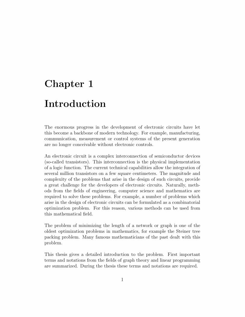
vertex of degree 1 is called a leaf or a pendant vertex. An edge incident to aleaf is a leaf edge or a pendant edge. A non-leaf vertex is an internal vertex.Sometimes, one vertex of the tree is distinguished, and called the root, inwhich case the edges have a natural orientation, towards or away from theroot. Such a tree is called a routed tree.

Figure 2.2: A labeled tree

In figure 2.2 a labeled tree with 6 vertices and 5 edges is shown. Nodes1, 2, 3, and 6 are leaves, while 4 and 5 are internal vertices.

2.1.4 Planar Graphs

A graph G = (V ,E ) can be drawn in a plane, by representing each vertexby a point in the plane, and assigns a curve or a straight line to each edge,that connects the points, which are representing the two end vertices of theedge. A graph is called planar if it can be drawn in the plane such that twoedges (more precisely, they representing curves) intersect at most in theirend vertices.

5

Figure 2.3: Planar and Non-Planar Graphs

Such a representation of a planar graph (Figure 2.3 (A)) in the plane iscalled an embedding of G in the plane. There can be different embeddingsfor a graph G . The example B is a non-planar graph, because the edges in-tersect with each other, it cannot reconfigured in a manner that would makeit planar.

When a graph is drawn without any intersection, any cycle that surroundsa region without any edges reaching from the cycle into the region forms aface. Two faces on a planar graph are adjacent if they share a common edge.A face that contains the entire graph is called outer face. In this thesis theouter surface of the graph G is denoted by the edge set OG .

2.1.5 Grid Graphs

A graph G = (V ,E ) is called a grid graph, if the set of vertices V can benumbered, such that V ⊆ {(i , j )|i = 1, ..., h; j = 1, ..., b} with (h, b) ∈ N×N.The number h is called the grid height and the number b, the grid width ofG . It is obvious that each grid graph is planar.

6

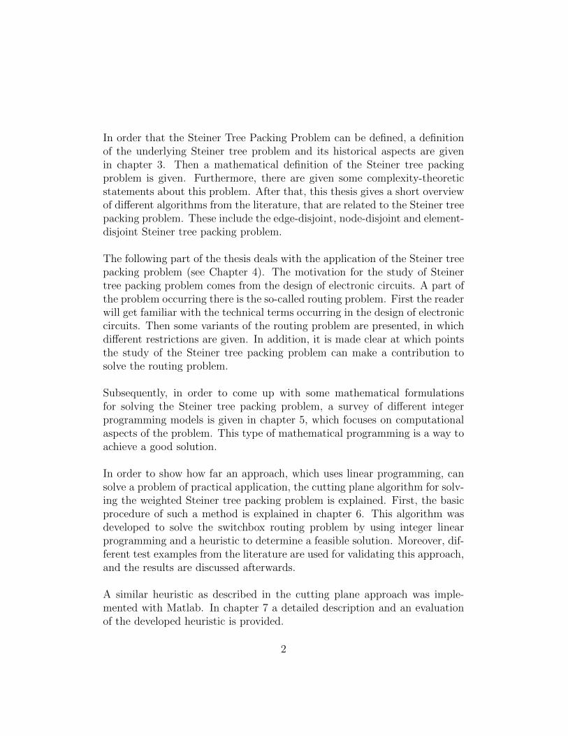
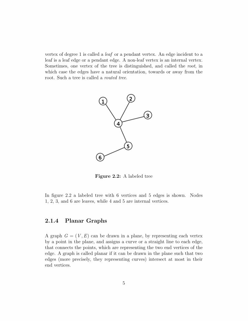
For a grid graph G it is normally assumed a certain embedding, in whicheach edge of the form [(i , j ), (i + 1, j )] is represented by an vertical line andeach edge of the form [(i , j ), (i , j + 1)] is represented by an horizontal line(Figure 2.4).

Figure 2.4: A Grid Graph

2.1.6 Hypergraphs

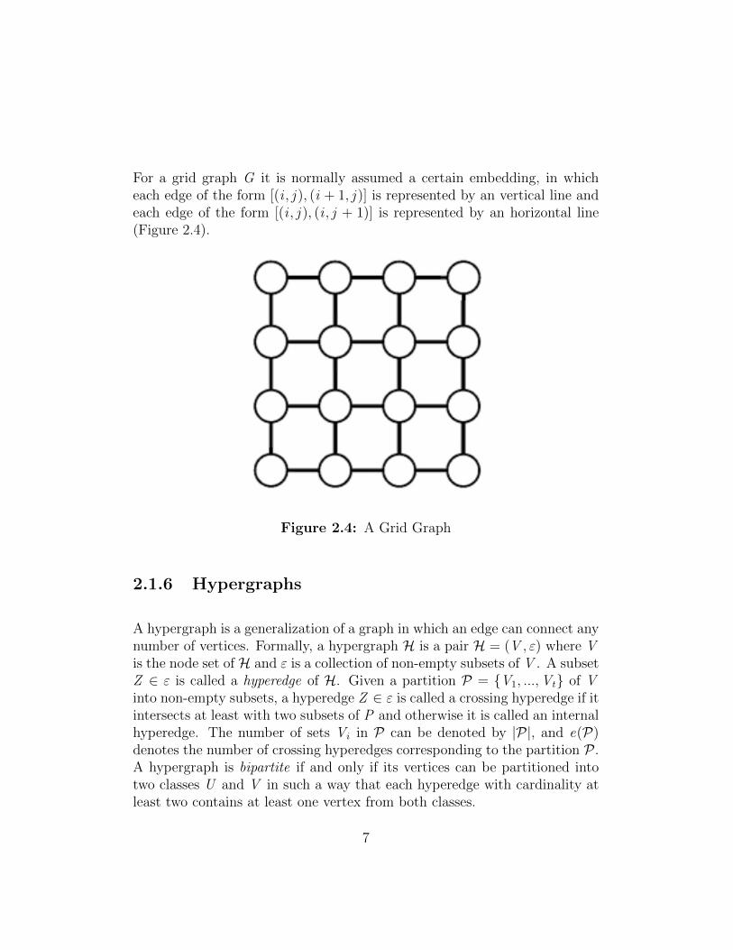
A hypergraph is a generalization of a graph in which an edge can connect anynumber of vertices. Formally, a hypergraph H is a pair H = (V , ε) where Vis the node set of H and ε is a collection of non-empty subsets of V . A subsetZ ∈ ε is called a hyperedge of H. Given a partition P = {V1, ...,Vt} of Vinto non-empty subsets, a hyperedge Z ∈ ε is called a crossing hyperedge if itintersects at least with two subsets of P and otherwise it is called an internalhyperedge. The number of sets Vi in P can be denoted by |P|, and e(P)denotes the number of crossing hyperedges corresponding to the partition P .A hypergraph is bipartite if and only if its vertices can be partitioned intotwo classes U and V in such a way that each hyperedge with cardinality atleast two contains at least one vertex from both classes.

7

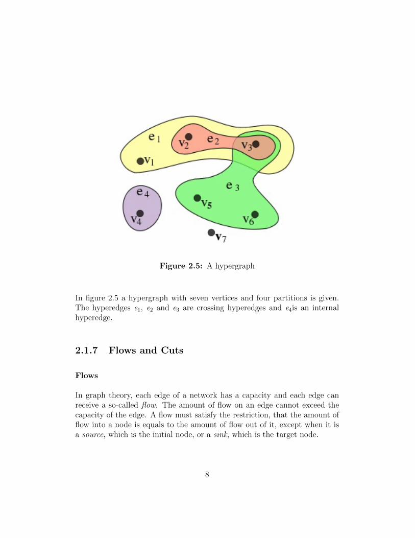
Figure 2.5: A hypergraph

In figure 2.5 a hypergraph with seven vertices and four partitions is given.The hyperedges e1, e2 and e3 are crossing hyperedges and e4is an internalhyperedge.

2.1.7 Flows and Cuts

Flows

In graph theory, each edge of a network has a capacity and each edge canreceive a so-called flow. The amount of flow on an edge cannot exceed thecapacity of the edge. A flow must satisfy the restriction, that the amount offlow into a node is equals to the amount of flow out of it, except when it isa source, which is the initial node, or a sink, which is the target node.

8

Given a directed graph G = (V ,E ) in which every edge (u, v) ∈ E hasa non-negative capacity c(u, v). If (u, v) /∈ E , it is assumed that c(u, v) = 0.A flow with the source s and the sink t is a function f : E → R≥0 with thefollowing three properties for all nodes u and v :

1) The capacity constraints f (u, v) ≤ c(u, v), which presupposes that theflow along an edge cannot exceed its capacity. The flow from u to v must bethe opposite of the flow from v to u.

2) The conservation constraint implies that∑w∈V

f (u,w) =∑w∈V

f (w , u), un-

less u = s or u = t . The flow to a node is zero, except for the source node,which produces flow, and the sink node, which consumes flow.

Notice that f (u, v) is the flow from u to v . If the graph represents a physicalnetwork, and if there is a real flow of, for example four units from u to v ,and a real flow of three units from v to u, then f (u, v) = 1.

Figure 2.6: A graph showing flow and capacity

In figure 2.6 a graph is shown, where the flow and capacity of an edge isdenoted by f /c.

9

Cuts

A cut is a partition of the vertices of a graph into two disjoint subsets.The cut-set of the cut is the set of edges, whose end points are in differentsubsets of the partition. Edges are said to be crossing the cut, if they are inits cut-set.

In a network the cut requires the source and the sink to be in different sub-sets. In this case the cut-set only consists of edges going from the source’sside to the sink’s side.

Figure 2.7: A cut on a graph

In figure 2.7 a cut is shown, where one partition has black vertices and theother partition has white vertices. The red edges are in the cut-set, becausetheir end points are in different subsets of the partition.

10

2.2 Linear Programming

Linear programming [Van08] (shorter: LP) is a mathematical method for de-termining a way to achieve the best outcome in a given mathematical modelfor some list of requirements represented as linear relationships. Linear pro-gramming is a specific case of mathematical programming.

More formally, linear programming is a technique for the optimization ofa linear objective function, subject to linear equality and linear inequalityconstraints. Let Ax ≤ b (Ax = b) be a system of linear inequalities (equal-ities), with A a real m × n - matrix and b ∈ R

m . The set of solutions{x ∈ R

n |Ax ≤ b} from a system of inequalities is then called the feasibleregion of the linear program, which is a polyhedron. It is a intersection offinitely many half spaces, each of which is defined by a linear inequality. Itsobjective function is a real-valued affine function defined on this polyhedron.A linear programming algorithm finds a point in the polyhedron, where thisfunction has the smallest (or largest) value if such a point exists.

Linear programs are problems, that can be expressed in the standard form:

minimize cTxsubject to Ax ≤ band x ≥ 0

x represents the vector of variables, which has to be computed, c and bare vectors of (known) coefficients and A is a (known) matrix of coefficients.The expression, which has to be minimized in this case is called the objectivefunction (here cTx ). The inequalities Ax ≤ b and x ≥ 0 are the constraintswhich specify a convex polyhedron over which the objective function is to beoptimized.

If all of the unknown variables are required to be integers, then the problem iscalled an integer programming or integer linear programming (shorter: ILP)problem. In contrast to linear programming, which can be solved efficientlyin the worst case, integer programming problems are in many practical situ-ations NP -hard. A special case, 0− 1 integer linear programming, in whichunknowns are binary, is one of the Karp’s 21 NP -complete problems.

11

Linear Programming Relaxation

The linear programming relaxation [MG07] (shorter: LP-Relaxation) of aninteger program is the problem, that arises by replacing the constraint xi ∈{0, 1}, that each variable must be either 0 or 1 by a weaker constraint0 ≤ xi ≤ 1, that each variable belong to the interval [0, 1].

The resulting relaxation is a linear program, hence the name. The relax-ation technique transforms an NP -hard optimization problem (integer pro-gramming) into a related problem, that is solvable in polynomial time (linearprogramming); the solution to the relaxed linear program can be used to gaininformation about the solution to the original integer program.

12

Chapter 3

Steiner Tree Packing Problem

In this chapter, a mathematical definition of the Steiner Tree Packing Prob-lem is given. In addition, some designations and properties are introduced,which will be useful later on. Some statements about the complexity of theproblem are given and, moreover, related problems from the literature arestudied.

3.1 Steiner Tree Problem

Before the Steiner Tree Packing Problem can be defined, the notion of Steinertree is needed. The actual Steiner tree problem will be discussed. Also thehistorical aspects of this problem are offered.

The Steiner problem is the combinatorial variant of the much older EuclideanSteiner problem, which asks for a minimal tree that connects a given set ofpoints in the plane. This problem has already been discussed, before 1640by Fermat [Str10]:

Given three points in the plain, find a fourth point T , such that the lengthfrom this point to the three given points is minimal.

13

Torricelli solved this problem and the point has since been known as theTorricelli-point. Torricelli’s method was to construct equilateral triangles oneach side of the triangle made up by the original points. Circles circumscrib-ing the equilateral triangles intersect in the point that is sought.

Jacob Steiner (1796-1863) considered a generalization of this problem forn points (the generalized Fermat problem), which is the origin of the (Eu-clidean) Steiner problem. These two problems are identical only in the casen = 3. In 1836 the Steiner problem is believed to have been presented first byGauß. The first (terminating) algorithm for the Euclidean Steiner problemwas given by Melzak [Mel61]. More information on the Euclidean Steinerproblem and its history is contained in Hwang et al. [HRW92].

In 1971 Hakimi and Levin, independently of each other, gave a formulationof the Steiner tree problem [Hak71, Lev71]. Since then hundreds of articleshave been published concerning different variants of this problem.

(Steiner Tree Problem)

Given: An undirected graph G = (V ,E ) with edge cost c : E → R+, anda set of vertices T ⊆ V , called terminals.

Problem: Find an edge set S spanning T of minimum cost c(S ) :=∑e∈S

c(e).

Given a set of terminals, a tree is called a Steiner tree, if all leafs are termi-nals. It combines all terminals and it is allowed to use non-terminal verticesof the graph (the Steiner nodes) in order to determine the Steiner tree.

To illustrate the difference between a graph, a Steiner tree and a minimumSteiner tree, all three variants are shown graphically in an example below.

14

Figure 3.1: An arbitrary graph

In figure 3.1 is shown a graph G , which has a set of vertices and a setof edges. The green squares are terminal symbols, the yellow circles are theother nodes and the connecting lines have to be seen as edges with assignedlength.

Figure 3.2: Steiner tree

This graph (Figure 3.2) is a Steiner tree, since it contains all the termi-nals and also all the leaves of the tree are occupied by terminal symbols.

15

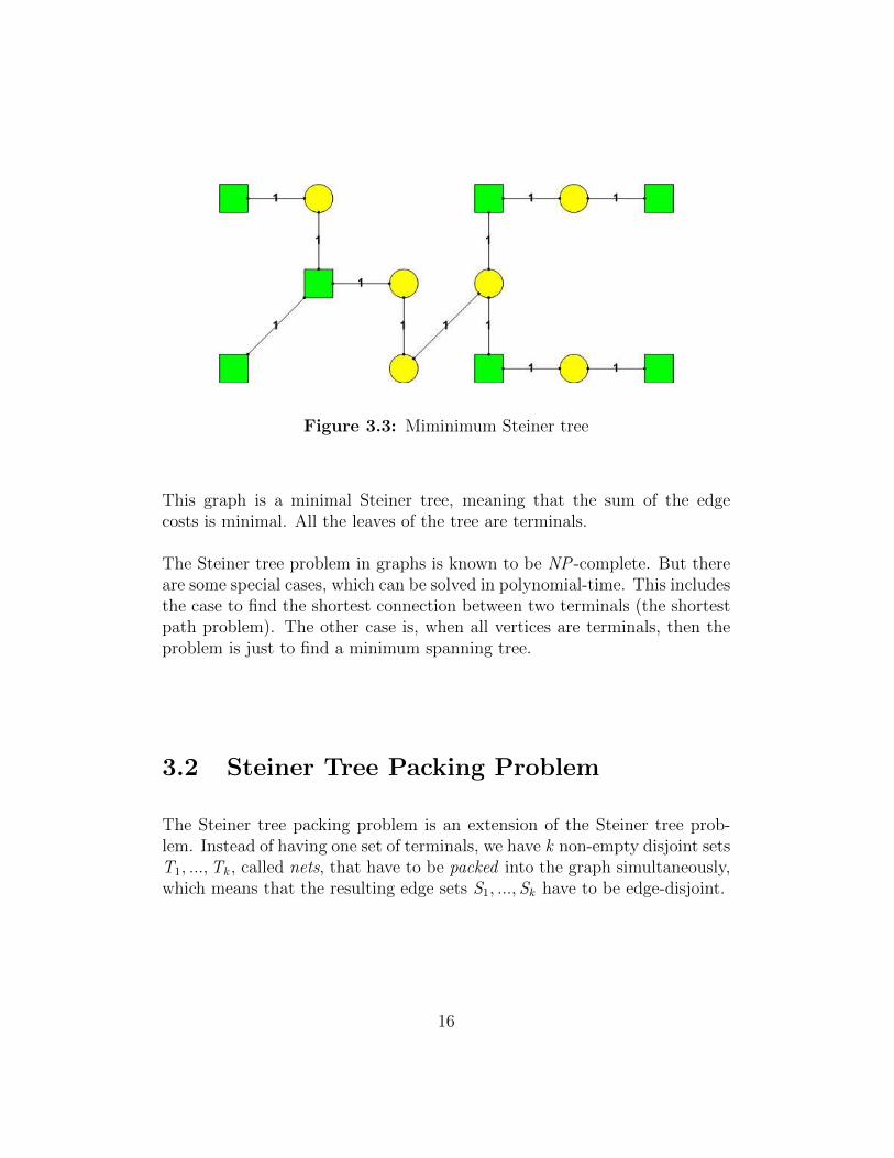
Figure 3.3: Miminimum Steiner tree

This graph is a minimal Steiner tree, meaning that the sum of the edgecosts is minimal. All the leaves of the tree are terminals.

The Steiner tree problem in graphs is known to be NP -complete. But thereare some special cases, which can be solved in polynomial-time. This includesthe case to find the shortest connection between two terminals (the shortestpath problem). The other case is, when all vertices are terminals, then theproblem is just to find a minimum spanning tree.

3.2 Steiner Tree Packing Problem

The Steiner tree packing problem is an extension of the Steiner tree prob-lem. Instead of having one set of terminals, we have k non-empty disjoint setsT1, ...,Tk , called nets, that have to be packed into the graph simultaneously,which means that the resulting edge sets S1, ..., Sk have to be edge-disjoint.

16

(Steiner Tree Packing Problem)

Given: A planar graph G = (V ,E ) and a list of terminal setsN = (T1, ...,TN ), where N ≥ 1 and Tk ⊆ V for all k = 1, ...,N .

Problem: Find for each k = 1, ...,N , an edge set Sk ⊆ E , which spans Tk ,such that (V (Sk), Sk) is a Steiner tree and S1, ..., SN are pairwiseedge-disjoint.

The list of vertex sets N is called a netlist. The number N denotes the cardi-nality of the netlist. A vertex set Tk is called a terminal set and the elementsof Tk terminals. All vertices, which are used by the edge set Sk , are denotedby V (Sk). It is often used net k instead of terminalset Tk . The notationsnet, terminal, etc. originate from the VLSI-Design (Chapter 4), which isthe main application area of the Steiner tree packing problem. Usually theedge capacities ce = 1, if ce > 1, the problem will be extended to multiplelayers. An instance of the Steiner tree packing problem is then defined bythe triple (G ,N , c). That means, when refering to an instance of a Steinertree packing problem, so a triple (G ,N , c) is always meant.

Often there are additionally given weighted edges, searching for a solution ofthis problem, which is minimal with respect to the weightings. This weightedproblem is called the weighted Steiner tree packing problem.

(Weighted Steiner Tree Packing Problem)

Given: A planar graph G = (V ,E ), with non-negative weighted edgeswe ∈ R+. A list of terminal sets N = (T1, ...,TN ), with N ≥ 1and Tk ⊆ V for all k = 1, ...,N .

Problem: Find for each k = 1, ...,N , an edge set Sk ⊆ E , which spans Tk ,such that (V (Sk), Sk) is a Steiner tree. The resulting edge setsS1, ..., Sk have to be edge-disjoint while the weighted sum ofN∑

k=1

∑e∈Sk

we have to be minimal.

The notation (G ,N , c,w) is an instance of the weighted Steiner tree packingproblem and is also called a weighted instance of the Steiner tree packingproblem.

17

3.3 Complexity

It is not surprising, that the (weighted) Steiner tree packing problem is NP -complete (NP -hard). In this context the decision problem, whether the prob-lem is solvable or not, is NP -complete and the optimization problem, wherean optimal solution is searched, is NP -hard. This problems has a lot of spe-cial cases, which are already NP -complete or NP -hard. In the following asmall selection of special cases is given.

The case N = 1 will be considered for the weighted Steiner tree packingproblem, such that the Steiner tree problem (Section 3.1) will be obtained.Karp [Kar10] showed that the Steiner tree problem is NP -hard. Garey andJohnson [GJ77] show that the so-called rectangular Steiner tree problem isalso NP -hard. For this problem several points are given in a plane and thegoal is to find a tree of minimum cost connecting the points with horizontaland vertical lines. From this it follows directly, that the Steiner tree prob-lem also remains NP -hard, when the underlying graph G is planar or a gridgraph and all edges have the same weights.

For example the Steiner tree packing problem contains the problem of findingk edge-disjoint paths. This problem is obtained if it is additionally requiredthat all terminal sets have a cardinality of two. Kramer and van Leeuwen[Kv80] have provided a proof of NP -completeness for this problem. Anotherspecial case of the Steiner tree packing problem arises, when only two termi-nal sets are specified. Also in this case this problem is NP -complete [KPS90].

Moreover, there are NP -complete problem statements for very specific in-stances, which very often occur in applications derived from the VLSI-Design(Chapter 4). Let G = (V ,E ) be a complete, rectangular grid graph and Na netlist, whose terminals are only located on the four borders of the gridgraph. Sarrafzadeh [Sar87] showed that it is NP -complete to decide, whetherthere is a Steiner tree packing for such a problem. This result remains valid,if each terminal set has at most cardinality k for a fixed k > 3. For the casek = 2, this problem can be solved in polynomial time.

These examples should give an impression about the actual difficulty of theproblem. It can be said that the (weighted) Steiner tree problem is NP -hard.There are also special cases, which can be solved in polynomial time.

18

3.4 Related Problems

The Steiner tree packing problem is a long studied topic. Here a shortoverview of different ideas and algorithms for the Steiner tree packing prob-lem is given. The various algorithms were divided roughly into the edge-disjoint, the vertex-disjoint and the element-disjoint cases.

3.4.1 Edge-Disjoint Steiner Tree Packing

The edge-disjoint case is usually treated, when referring to a Steiner treepacking problem. Most of the edge-disjoint Steiner tree packing problems inplanar graphs are NP -complete. Even when restricted to paths, which means,that all nets have only two terminals, the problem remains NP -complete. Inthe following some algorithms of this problem are presented.

(Max-Steiner-Tree-Packing Min-Steiner-Cut Algorithm)

This approximation algorithm for the Steiner tree packing problem was givenby Lau [Lau07]. The goal is to find a largest collection of edge-disjoint Steinertrees of an undirected graph G . In this approximation algorithm the mainidea is an approximate min-max relation between the maximum number ofedge-disjoint Steiner trees, that each connect the terminals and the minimumsize of an edge-cut that disconnect some pair of terminals.

Given an undirected graph G and a subset of vertices S ⊆ V (G), calledterminals. The terminals S are also called black vertices, while the verticesV (G)\S are called white vertices (Steiner vertices). An edge is called a whiteedge if it connects two white vertices.

The algorithm consists of two parts. In the first step the given graph G with` white edges will be transformed into at most ` + 1 graphs {G1, ...,G`+1},such that each graph has no white edge by using Edmonds’ matroid par-tition algorithm [Edm65]. In the second step for each subgraph Gi withi = 1, ..., ` + 1, all Steiner trees are determined. Afterwards the solutions ofthe subgraphs are combined.

19

Then the Steiner tree packing problem is formulated by the following linearprogram, which was introduced by Jain, Mahdian and Salacatipour [JMS03]:

maximize∑T∈T

xT

subject to∑T∈Te∈E

xT ≤ ce ∀T ∈ T : xT ≥ 0

In this formulation T denotes the collection of all Steiner trees in a graphG = (V ,E ), and ce is the given capacity of the edge e ∈ E . The size of Tgrows exponentially to the number of vertices in V .

(Edge-Disjoint Steiner Trees)

This approximation algorithm for packing edge-disjoint Steiner trees in pla-nar graphs was introduced by Aazami [Aaz08]. Based on the element-disjoint Steiner tree packing algorithm (Section 3.4.3), which also was givenby Aazami, this egde-disjoint version of the problem on planar graphs wasdeveloped. The goal is to find a maximum cardinality set of edge-disjointSteiner trees, such that each tree contains every terminal node.

A graph is said to be k -edge connected if it remains connected wheneverat most k edges are removed. The following statement is the main result ofthis algorithm:

Let G = (V ,E ) be an undirected planar graph, let R ⊆ V be the set ofterminals, and assume that R is k-edge connected. Then there are at leastb k4c−1 edge-disjoint Steiner trees in G. Moreover, there is an algorithm with

a running time of O(|V |4.5) that finds at least b k4c − 1 edge-disjoint Steiner

trees in G.

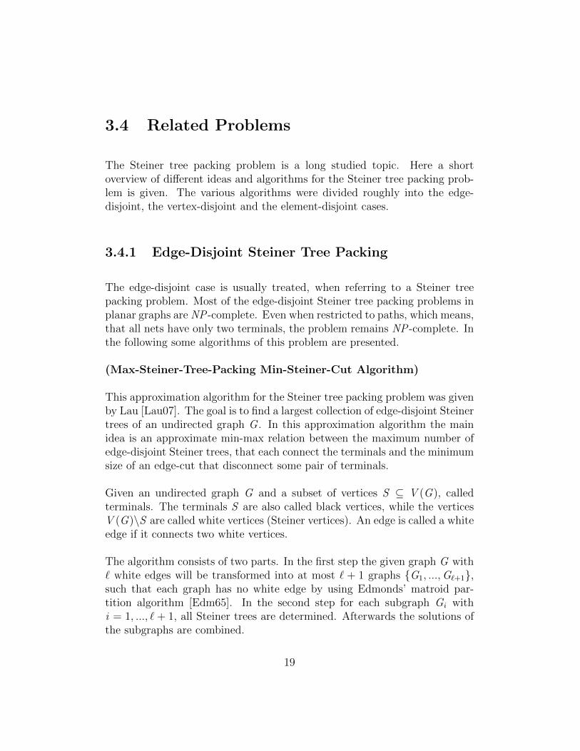
The graph G is first reduced to a planar graph G ′ with Steiner nodes ofdegree at most four. To achieve this, a Steiner node of degree more than fouris repeatedly replaced by a so-called gadget, which retains the connectivity

20

and planarity. The gadget and its properties are well known from the liter-ature [MP93, NS08]. The new Steiner nodes have a degree of at most four.For example let v be a Steiner node of degree seven in G . The node will bereplaced by a gadget as shown in figure 3.4.

Figure 3.4: Gadget for high degree nodes [Aaz08]

Let v be a Steiner node of degree d > 4 in G . The gadget has dd2e − 1

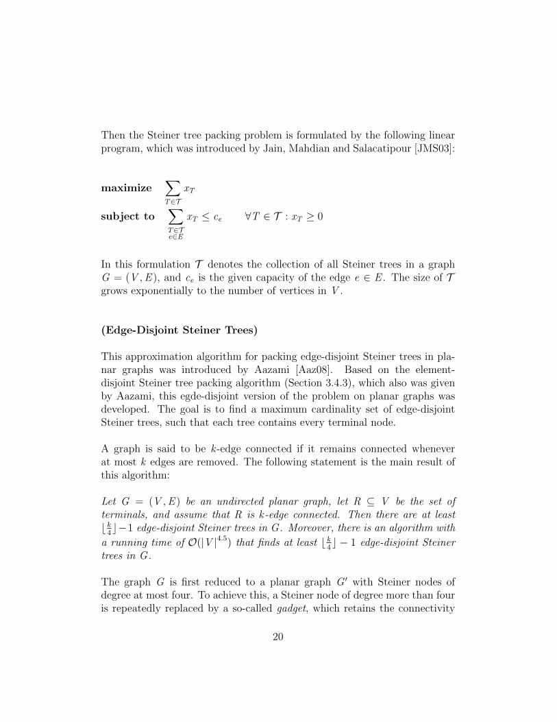
rows including the row with the previously given Steiner node, which is nowcalled v ′. Through this process the graph now has one less Steiner node ofdegree more than four. The set of terminal nodes and their degree stay thesame. Any set of edge-disjoint paths using edges which belongs to v can bererouted via the gadget (Figure 3.5).The set of terminals R is k -connected inthe obtained graph, where every Steiner node is of degree less or equal four.

Figure 3.5: Routing paths via the gadget [Aaz08]

21

Given a pairing of edges, used in the paths, going through v , one of the ex-treme pairs will be routed first. An extreme pair is the pair, which uses theleft most edge or the right most edge. This pair uses the first horizontal rowof the gadget. The next pair is routed along the vertical edges to the nexthorizontal row. Some of the paths may be need to be shifted, like the pathlabeled (2, 2′), which is shifted on the first row to the left (Figure 3.5).

An edge that connects two terminals can be subdivided by introducing aSteiner node. Aazami assumes that G ′ does not contain such an edge con-necting two terminals. By applying the element-disjoint Steiner tree packingalgorithm (Section 3.4.3) to G ′, there are b k

4c − 1 element-disjoint Steiner

trees in G ′. These Steiner trees are obviously edge-disjoint. Then it can besaid that G has at least b k

4c − 1 edge-disjoint Steiner trees.

3.4.2 Vertex-Disjoint Steiner Tree Packing

In the vertex-disjoint case, each node of the graph G is only allowed to occurin one of the Steiner trees. The vertex-disjoint Steiner tree packing problemin planar graphs is known to be NP -complete. Even when restricted to paths,which means that all nets have only two terminals, the problem remains NP -complete. Robertson and Seymour [RS90] showed, that the vertex-disjointpaths packing problem is solvable in polynomial time if the number of paths kis fixed. A linear-time algorithm for planar graphs, which goodness stronglydepends on the number of paths, has been introduced by Reed, Robertson,Schrijver and Seymour[RRSS93].

There are polynomial time algorithms for the vertex-disjoint Steiner treepacking problem in planar graphs, where the terminals lie only on one or twoborders of the graph. The algorithms, which are presented in the following,where the terminals lie only on one border of the graph may be seen as a keyidea for simple linear-time algorithms for similar problems.

22

(Vertex-Disjoint One-Face Steiner Tree Packing Problem)

Given: A planar graph G = (V ,E ), |V | = n, and pairwise vertex-disjointsets N1, ...,Nk ⊆ V . The graph G is embedded in the plane, suchthat all terminals lie on the boundary of the outer face of G .

Problem: Find, for each i = 1, ..., k , a Steiner tree Ti for Ni such thatTi , ...,Tk are pairwise vertex-disjoint.

It should be noted, that in this problem statement a feasible not an optimalsolution is searched. The algorithm, given by Liao and Sarrafzadeh [LS91],has two steps. In the first step the topological solvability is tested and in thesecond step the layout of the nets is determined. It is important that enoughedge capacity is available and that the nets have a nested structure, whichmeans that the nets are not allowed to intersect each other. The topologicalsolution is a collection of Steiner trees for the nets that can be drawn dis-jointly in the plane outside the outer face.

The topological solvability can be decided by the simple Stack Algorithm.It checks whether the nets are nested. In this algorithm the terminals arescanned in anti-clockwise direction along the outer face boundary, beginningwith some arbitrary terminals. Every new visited terminal is pushed ontothe stack. If the pushed terminal is the last non-visited terminal of the cor-responding net, it is tested if all terminals of the net lie on top of the stack.If this is not the case, the problem is not topologically solvable. Otherwise,all terminals of the net are popped. When all the terminals of all nets arevisited, and there was no conflict before, the instance is topologically solvableonly if the stack is empty. For net Ni the first terminal is denoted by si andthe last terminal by ti .

Stack Algorithm

Input:A net set N = {Ni |i = 1, ..., k} and a planar graph G , where si and ti areon the outer face.STACK := ∅

23

Output:Topological solvable or unsolvable.

beginarbitrarily choose a vertex v as the starting point;the first terminal si is the one closest to v in anti-clockwise direction of theboundary of G ;set j = i and a = |Nj | − 1;walk anti-clockwise direction along outer face boundary;if visited vertex v ∈ Nj ;

then a = a − 1;if a = 0, such that v is a last terminal ti ;

then POP until si is popped;else if a 6= 0;

then PUSH v on the stack;else if v ∈ Nk for k 6= j and a 6= 0;

then return topological unsolvable;else if v ∈ Nk for k 6= j ;

then j = k and a = |Nj | − 1;end;

return topologically solvable;

The Stack Algorithm can be implemented to run in linear time. The one-facelayout algorithm, which tries to get a solution, is now based on the StackAlgorithm. This algorithm is explained in the following. In order to get acorrect spanning of the nets, they are considered in the order, in which theyhave been deleted from the stack. After a net is routed, the boundary iscorrected by deleting all used edges and vertices, and all edges incident tothem.

(One-face Layout Algorithm)

This algorithm can be interpreted as a right-first search or a depth-firstsearch, where in each search step the edges are searched from right to left.A backtrack and remove step consists of a backtrack step, where in additionthe searched edge is deleted from the graph. For technical reasons all si aredetermined to have degree one in G . In the following the One-Face LayoutAlgorithm is formulated:

24

Algorithm

for i := 1 to k dolet pi initially consist of the unique edge incident to si ;v := the unique vertex adjacent to si ;while not all terminals of Ni are visited and v 6= si do

if at least one edge incident to v is not yet searched thenlet {v ,w} be the next edge after the leading edge of pi w.r.t. v ;if w is just occupied by some tree different from Ni then

perform a backtrack and remove step;else add {v ,w} to pi ;v := w ;

else perform a backtrack and remove step;v := the leading vertex of pi ;

if v = si then stop; return unsolvable;return (p1, ..., pk);

The running time of this algorithm is also O(n).

3.4.3 Element-Disjoint Steiner Tree Packing

This approximation algorithm for packing element-disjoint Steiner trees inplanar graphs was introduced in [Aaz08]. An element describes either anedge or a Steiner node. The goal is to find a maximum cardinality set ofelement-disjoint Steiner trees, such that each tree contains every terminalnode. The method consists of two steps. In the first step the given graphG will be transformed into a bipartite graph. In the second step the bipar-tite graph is considered as a hypergraph and apply a method of Frank et al.[FKK03] to decompose the set of hyperedges ε into a number of disjoint setsε1, ε2, ε3, ..., where each set is a Steiner tree of the bipartite graph. Each ofthese bipartite Steiner trees will be transformed back to a Steiner tree of theoriginal graph.

A graph is k -element connected if it remains connected whenever at mostk edges or Steiner nodes are removed. The following statement is the mainresult of this algorithm:

25

Let G = (V ,E ) be an undirected planar graph, let R ⊆ V be the set of ter-minals, and assume that R is k-element connected. Then there are at leastb k2c − 1 element-disjoint Steiner trees in G. Moreover, there is an algorithm

with a running time of O(|V |4.5) that finds at least b k2c − 1 element-disjoint

Steiner trees in G.

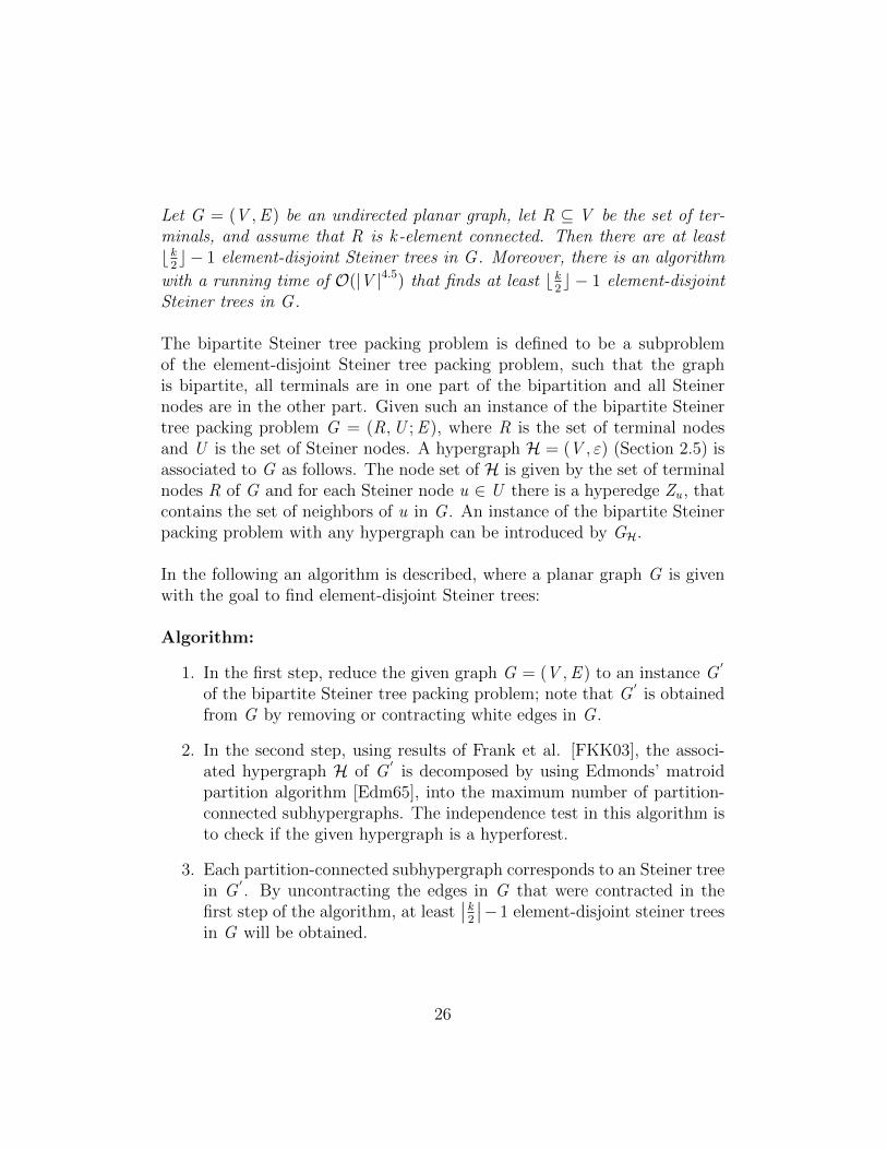
The bipartite Steiner tree packing problem is defined to be a subproblemof the element-disjoint Steiner tree packing problem, such that the graphis bipartite, all terminals are in one part of the bipartition and all Steinernodes are in the other part. Given such an instance of the bipartite Steinertree packing problem G = (R,U ; E ), where R is the set of terminal nodesand U is the set of Steiner nodes. A hypergraph H = (V , ε) (Section 2.5) isassociated to G as follows. The node set of H is given by the set of terminalnodes R of G and for each Steiner node u ∈ U there is a hyperedge Zu , thatcontains the set of neighbors of u in G . An instance of the bipartite Steinerpacking problem with any hypergraph can be introduced by GH.

In the following an algorithm is described, where a planar graph G is givenwith the goal to find element-disjoint Steiner trees:

Algorithm:

1. In the first step, reduce the given graph G = (V ,E ) to an instance G′

of the bipartite Steiner tree packing problem; note that G′

is obtainedfrom G by removing or contracting white edges in G .

2. In the second step, using results of Frank et al. [FKK03], the associ-ated hypergraph H of G

′is decomposed by using Edmonds’ matroid

partition algorithm [Edm65], into the maximum number of partition-connected subhypergraphs. The independence test in this algorithm isto check if the given hypergraph is a hyperforest.

3. Each partition-connected subhypergraph corresponds to an Steiner treein G

′. By uncontracting the edges in G that were contracted in the

first step of the algorithm, at least∣∣ k2

∣∣−1 element-disjoint steiner treesin G will be obtained.

26

Chapter 4

VLSI-Design

The motivation for the study of Steiner tree packing problem comes fromthe field of the design of electronic circuit, which is also called Very LargeScale Integration (shorter: VLSI). An important subproblem that occursin the design of electronic circuits is the routing problem. In this chapter,the routing problem is considered in more detail. The problems which ariseare identified and some solution approaches are given [JLPP02, GMW96a,GMW97, KH12].

4.1 Routing Problem in VLSI-Design

The VLSI-Design can be divided into two phases. A circuit has to fulfill agiven task. The task is a complex logical function, which is comprised ofmany elementary logical operations. The logical design specify, which of thelogical functional units may be used and defines the connection, which haveto be realized between the units. These units specifying a logical functioncalled cells. The connections, which have to be realized are called networks.The list of cells, together with the list of networks, forms the input for thesecond phase, the physical design. The task here is to realize the logicaldesign physically, this means that the cells have to be arranged on a givensurface and to realize the network, which is connected by electrical lines. Thetask is made more difficult, because depending on the technology specific de-sign rules (for example: minimum distance of certain cells or networks) mustbe observed and an objective function, where the resulting surface must beminimized. Generally this problem can be divided into two subproblems,

27

which are solved one after the other. The first is the placement problem,which deals with the arrangement of the cells and the second is the routingproblem, which deals with the realization of the network. In this thesis onlythe routing problem is from intrest.

As mentioned above, the routing problem is to connect the cells on the rout-ing area subject to certain technical side constraints. The objective usually isto minimize the overall routing length. A net is called routed if its terminalsare connected. A net where k is the number of terminals, is defined as ak-terminal net. If k > 2, the term multiterminal net is often used.

For the routing there are usually several levels available, the so-called layers.If a net changes a layer, a hole must be drilled. Such a hole is called a via.The routing of a net is usually on horizontal and vertical lines, the so-calledtracks to which the contacts of the nets must be assigned. If the routing ofthe nets is not on such tracks, this can also be called a grid-free routing.

4.2 Decomposition of the Routing Problem

In practice, the routing problem is usually decomposed, so that large scales,which can occur at this problem, can be treated. In a first step, the networkshomotopy is determined. It is defined how the cells have to be connected.This step is also known as the global routing. The second step is the detailedrouting. Here the nets are assigned to the layers and tracks according tothe homotopy specified in the global routing step. This decoposition schemegives rise to many variants of the routing problem.

4.2.1 Global Routing

For modelling the global routing problem, the routing area is subdivided intosubareas and these are represented by nodes in a graph. There are many vari-ants to make such a subdivision, which among other things depends on theunderlying technology and the methods used. An example of how such anrouting area may be divided is illustrated in figure 4.1.

28

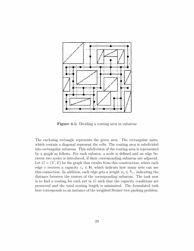
Figure 4.1: Dividing a routing area in subareas

The enclosing rectangle represents the given area. The rectangular units,which contain a diagonal represent the cells. The routing area is subdividedinto rectangular subareas. This subdivision of the routing area is representedby a graph as follows. For each subarea, a node is defined and an edge be-tween two nodes is introduced, if their corresponding subareas are adjacent.Let G = (V ,E ) be the graph that results from this construction, where eachedge e receives a capacity ce ∈ N, which indicats how many nets can usethis connection. In addition, each edge gets a weight we ∈ R+, indicating thedistance between the centers of the corresponding subareas. The task nowis to find a routing for each net in G such that the capacity conditions arepreserved and the total routing length is minimized. The formulated taskhere corresponds to an instance of the weighted Steiner tree packing problem.

29

4.2.2 Detailed Routing

After having solved the global routing problem, the detailed routing problemmust be solved. This means, that every subarea, which are represented bynodes and are connected by edges, must be routed in detail. The homotopy,which was determined at the global routing, must be considered. There area lot of different detailed routing models which are studied in the literature.In most cases, these problems can be formulated in a grid graph. This thesiswill be restricted to problems in such grid graphs.

The detailed routing problem can be classified according to two indepen-dent criteria. In the following the two (A, B) criteria are explained andvarious models are introduced.

A: Structure of the routing areaOne criterion distinguishes the detailed routing problems in the constructionof the routing areas. In the following different resulting models are presented:

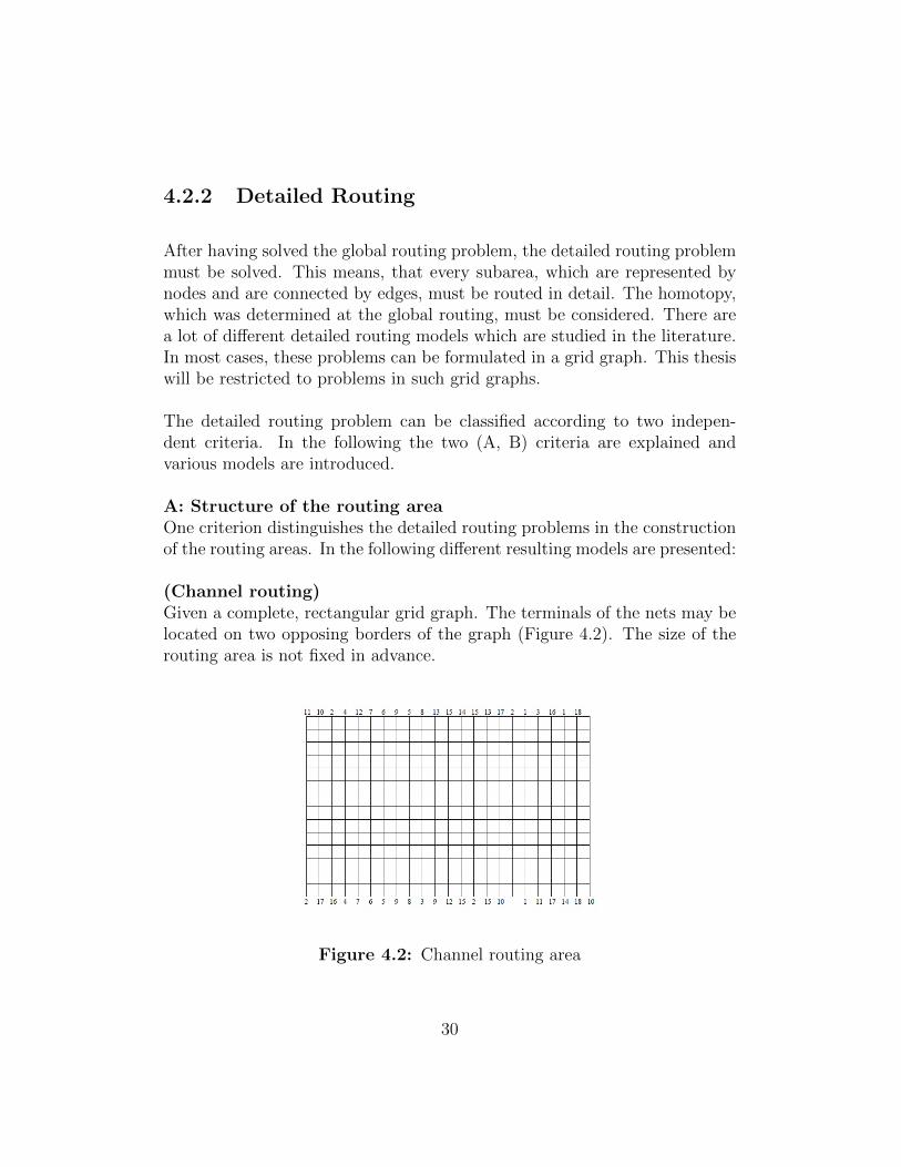
(Channel routing)Given a complete, rectangular grid graph. The terminals of the nets may belocated on two opposing borders of the graph (Figure 4.2). The size of therouting area is not fixed in advance.

Figure 4.2: Channel routing area

30

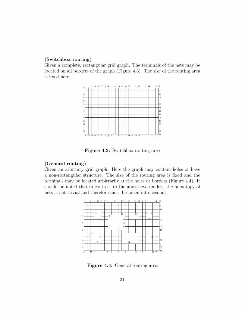
(Switchbox routing)Given a complete, rectangular grid graph. The terminals of the nets may belocated on all borders of the graph (Figure 4.3). The size of the routing areais fixed here.

Figure 4.3: Switchbox routing area

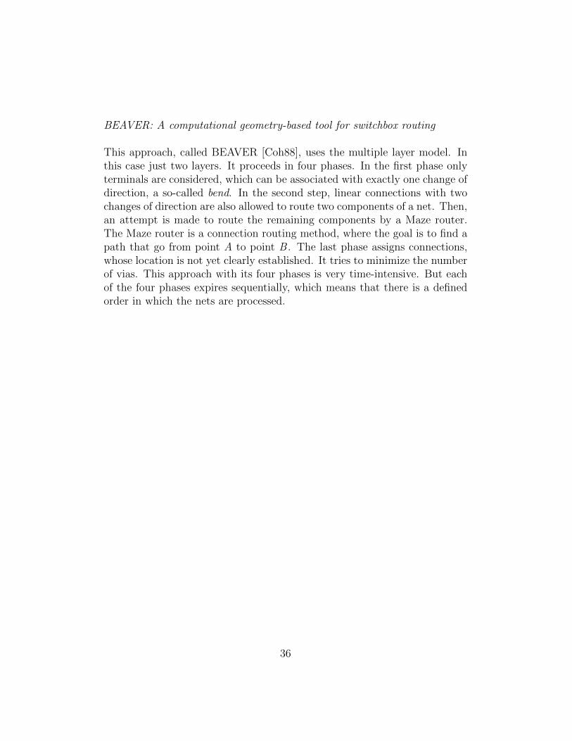
(General routing)Given an arbitrary grid graph. Here the graph may contain holes or havea non-rectangular structure. The size of the routing area is fixed and theterminals may be located arbitrarily at the holes or borders (Figure 4.4). Itshould be noted that in contrast to the above two models, the homotopy ofnets is not trivial and therefore must be taken into account.

Figure 4.4: General routing area

31

B: Layer structuresThe other criterion distinguishes the detailed routing problems by extent towhich the layers are taken into account when the connections of the netsare assigned to the tracks. In the following are presented different resultingmodels for this criterion:

(Multiple layer model)A k -dimensional grid graph can be obtained by stacking k copies of a gridgraph on top of each other and connecting the corresponding nodes by per-pendicular lines. The nets have to be routed in a node-disjoint way. Thismodel certainly comes very close to the technology requirements, but hasthe disadvantage that, in general, the resulting graphs are very large. Thenumber k has to be chosen minimal.

(Manhattan model)Given a planar grid graph. The nets have to be routed in a node-disjointway, with the additional restriction that nets that meet at some node arenot allowed to bend at this node. The so-called knock-knees are not allowed(Figure 4.5).

(Knock-knee model)Given a planar grid graph. The task is to find an edge-disjoint routing of thenets. Here the restriction of the Manhattan model is omitted, which meansthat knock-knees are allowed. It often arise shorter connections, than in theprevious model, but the main disadvantage is that the assignement to layersis neglected. Brady and Brown have designed an algorithm, that guarantees,that any solution in this model can be routed on four layers [BB84]. It wasshown, that it is NP -complete to decide if a realization on three layers ispossible.

Figure 4.5: Knock-knee model

32

These two types of categorization (A and B) with its models can be combinedarbitrarily. For example, the switchbox routing problem in the knock-kneemodel, which will be of interest in the approach presented in chapter 6. Ingraph-theoretic terms this combination can be formulated as a problem offinding edge-disjoint Steiner trees in a complete grid graph, where all termi-nals may be located on all borders of the graph. Additionally is the fact thatdepending on the model different objective functions can be optimized. Pos-sible objective functions are, minimizing of the routing area, minimizing ofthe routing length or minimizing the number of vias. In the case of switchboxrouting, minimizing of the routing length is typically the objective, becausehere the routing area is fixed. The objective for the channel routing problemis usually the minimization of the routing area and for the general routingproblem the minimization of the number of vias can be used as the objectivefunction.

4.3 Related Problems

As seen in this chapter, a large number of subproblems of the routing problemcan be derived. For all these models different approaches are studied and dis-cussed in the literature. In this section different approaches for the switchboxrouting problems, which are formulated as an instance of the Steiner treespacking problem, are given.

4.3.1 Switchbox routing

(Exact Method)

In this context an exact method is understood as an algorithm that alwaysfinds a solution, if there exists a solution or it decides in finite time that thereis no solution. Until now exact methods for the switchbox routing problemare known for the case, where only two terminals have to be routed in theknock-knee model. Because in this case the problem, to route N nets, isequivalent to the edge-disjoint packing problem.

33

Given a planar graph G = (V ,E ) and a net list N = {T1,T2, ...,TN} withTK = {sk , tk} for k = 1, 2, ...,N . The outer face of G is denoted by theedge set OG . Robertson and Seymour [RS90] denoted f (X ) = δG(X ) as aninduced cut X ⊆ V , where δG(X ) is the set of edges in G with one end nodein X and another in V \X (see Section 2.1.7). In the following an algorithmis described:

Algorithm

Input:A planar graph G = (V ,E ) and a net list N of nets {sk , tk} with k =

1, ..,N .Output:

N edge-disjoint paths P1,P2, ...,PN , such that sk and tk are connectedthrough Pk for k = 1, 2, ...,N , else there exists no solution.

(1) if G is not 2-vertex-connected, decompose G in components, whichare 2-vertex-connected and use the following steps on everycomponent

(2) let e ∈ OG be an edge, located in an induced cut of X , which isminimal regarding f

(3) if f (X ) < 0, then STOP (there exists no solution)(4) number V (OG) cyclically, such that V (OG) = {v0, v1, ..., vk = v0} with

e = v0v1(5) if f (X ) = 0, then(6) choose a vertex minimal cut X

′with vi ∈ X

′and v0 /∈ X

′;

(7) choose [vi , vj ] ∈ δH (X′) with vj /∈ X

′, j maximum;

(8) if f (X ) > 0, then(9) choose [vi , vj ] ∈ F arbitrarily;(10) set G := G\e and N := N\{vi , vj} ∪ {{vj , v0}, {vi , v1}}(11) if E 6= ∅, go to (1)(12) if sk 6= tk for {sk , tk} ∈ N , then STOP (there exists no solution)(13) identify the paths P1,P2, ...,PN according to the decomposition in (10)(14) STOP.

34

The difficult part of this algorithm is to show, that the choice of the cutX in step (6) and the choice of the nets in step (7) guarantee, that G\e andN := N\{vi , vj} ∪ {{vj , v0}, {vi , v1}} are solvable, if G and N are solvabletoo. The reduction of the problem in step (10) ensures, that N ⊆ V (OG).Finally, it should be noted for determining the ways in step (13), that theway P with the terminals {vi , vj} in step (10) is made up of the ways P1 with{vj , v0}, the way P2 with {vi , v1} and the edge e.

(Heuristics)

A heuristic is a technique designed for solving a problem more quickly whenclassic methods are too slow, or for finding an approximate solution, whenclassic methods fail to find any exact solution. This is achieved by tradingoptimality, completeness, accuracy, or precision for speed. In this sectionsome heuristic methods are described.

A greedy switch-box router

This approach introduced by Luk [Luk85] uses the Manhattan model for theswitchbox routing problem. Luk tries to extend a channel routing algorithmto a switchbox routing problem. The idea is to pass through the columnsof the routing area from left to right. In each column (iteration) the netsare assigned to the horizontal tracks. The nets, that already use horizontaltracks will be routed by taking into account the terminals, which have to beconnected. Nets, which have a terminal in the current column are assignedto free horizontal tracks. If there are not enough horizontal tracks, then ad-ditional tracks will be introduced. Also, additional columns are inserted atthe end, if the rightmost terminals can not be connected. Every decision ofthe algorithm is based on very heuristic arguments. This is especially truefor the selection of the direction (from left to right, top to bottom, or in eachcase vice versa) in which the grid graph is traversed.

35

BEAVER: A computational geometry-based tool for switchbox routing

This approach, called BEAVER [Coh88], uses the multiple layer model. Inthis case just two layers. It proceeds in four phases. In the first phase onlyterminals are considered, which can be associated with exactly one change ofdirection, a so-called bend. In the second step, linear connections with twochanges of direction are also allowed to route two components of a net. Then,an attempt is made to route the remaining components by a Maze router.The Maze router is a connection routing method, where the goal is to find apath that go from point A to point B . The last phase assigns connections,whose location is not yet clearly established. It tries to minimize the numberof vias. This approach with its four phases is very time-intensive. But eachof the four phases expires sequentially, which means that there is a definedorder in which the nets are processed.

36

Chapter 5

Integer Programming Models

In this chapter different, mathematical formulations for the Steiner tree pack-ing problem are given. A survey of these integer programming models canbe found in [Cho94]. In the following the same notations as introduced insection 3.2 is used.

5.1 The Undirected Cut Formulation

This formulation is used by Grotschel et al. in [GMW97]. A similar formu-lation as presented here, is given by Lengauer and Lugering in [Len90] and[LL93].

Given a weighted instance of the Steiner tree packing problem (G ,N , c,w).In addition binary variables χk

e are introduced, for all k = 1, ...,N and e ∈ E .

χke =

{1 if edge e is in the Steiner tree spanning net k ,

0 otherwise.

Each partitition (W ,V \W ) of the nodes V of the graph G defines a cut. Itis called a Steiner cut for net k if |W ∩Tk | ≥ 1 and |Tk\W | ≥ 1. Steiner cutsare based on the idea that a Steiner tree contains a path from the terminalt ∈ Tk to every other terminal Tk\{t}. Thus every cut separating the ter-

37

minal t from any other terminal Tk\{t} must contain at least one edge fromthe Steiner tree. Let δ(W ) be the set of edges in G with one end node inW and another in V \W . For a net k with k = 1, ...,N and each associatedSteiner cut (W ,V \W ), the Steiner cut inequality is defined. In generel theSteiner cut inequalities ensure that for each terminal set Tk , all Steiner cutsare covered with at least one edge.

In order that the capacity is large enough to satisfy the requirements ofall connections, which have to be housed, the capacity inequalities are in-troduced. It can also be said that by using capacities on the edges theformulation can be extended to model an arbitrary number of layers.

In the following an integer programming formulation to model an edge-disjoint routing for the weighted Steiner tree problem is given:

minN∑

k=1

∑e∈E

weχke

(i)∑

e∈δ(W )

χke ≥ 1, for all W ⊂ V , W ∩ Tk 6= ∅, Tk\W 6= ∅.

(ii)N∑

k=1

χke ≤ ce , for all e ∈ E .

(iii) χke ∈ {0, 1}, for all e ∈ E , k = 1, ...,N .

In the above mentioned integer programming model the inequalities (i) arecalled Steiner cut inequalities and inequalities (ii) are called capacity inequal-ities. The model can be further strengthened with several valid inequalities,which are described by Grotschel et al. in [GMW96a, GMW97, GMW96b].

This formulation contains only |E |+ |E |×N variables, but exponential manyinequalities (order of N × 2|V | constraints of type (i)).

38

5.2 The Directed Cut Formulation

This formulation was introduced by Wong in [Won84]. A similar formulationas presented here, is given by Bienstock and Bley in [BB00] or by Althaus,Polzin and Daneshmand in [APD03].

Given a weighted instance of the Steiner tree packing problem (G ,N , c,w),the formulation can be restated on a corresponding directed graph as follows:Given G = (V ,E ) with edge set E , construct the directed graph D = (V ,A)with arc set A, where arcs a = (s , t) and a ′ = (t , s) are in A if and onlyif edge e = st ∈ E . For each k ∈ N one vertex rk ∈ Tk will be chosen asroot. An arborescence is a directed, rooted tree in which all edges point awayfrom the root, such that an arborescence rooted at rk is said to be a Steinerarborescence, if it spans each node in Tk . A routing on D consists of a set ofSteiner arborescences with one for each net. In the following the variable yk

a

for each net k and arc a ∈ A are introduced:

yka =

{1 if arc a is in the Steiner arborescence spanning net k ,

0 otherwise.

In the following an integer programming formulation of the directed ver-sion is given:

min∑a∈A

N∑k=1

weyka

(i)∑

a∈δ(W )

yka ≥ 1, for all W ⊂ V , W ∩ Tk 6= ∅, Tk\W 6= ∅.

(ii)N∑

k=1

(yka + yk

a ′) ≤ ce , for all a ∈ A.

(iii) yka ∈ {0, 1}, for k = 1, ...,N .

Define a cut (W ,V \W ) to be a directed Steiner cut if rk ∈ W with |W ∩Tk | ≥ 1 and |Tk\W | ≥ 1. Define δ(W ) to be the set of arcs directed fromW to V \W with one end in W and the other in V \W . For each net k

39

and directed Steiner cut (W ,V \W ), the directed Steiner cut inequality (i)is obtained.

Consider an undirected edge e = st ∈ E and let a = (s , t) and a ′ = (t , s) bethe corresponding arcs in A. The capacity is consumed, if either a or a ′ arecontained in the directed routing. The capacities inequalites for this modelare given in inequalities (ii) [Cho94].

5.3 The Explicit Formulation

This formulation has been considered by Lengauer and Lugering [LL93]. Asimilar formulation has also been considered by Raghavan and Thompson[RT87].

Here the notation is a bit different as in the other formulations. The ideais that for each set of edges, which is a Steiner tree with respect to a ter-minal set a variable is introduced. Let Si = {Tij |j = 1, ..., ni} be the setof all possible Steiner trees in the graph G = (V ,E ), where Ti1,Ti2, ...,Tini

is an enumeration of the spanning tree of the ith terminal set. ni may beexponential in |V |. In this formulation a variable zij for each Steiner treeTij for net i is explicity defined. In the following the variable zij is introduced:

zij =

{1 if Steiner tree Tij is chosen to span net i ,

0 otherwise.

The total number of variables, where k is the number of terminal sets, isgiven by:

k∑i=1

ni

The weight lij of a Steiner tree Tij is given by:

lij =∑e∈Tij

we

40

In the following an integer programming formulation of the explicit versionis given:

mink∑

i=1

ni∑j=1

lij zij

(i)

ni∑j=1

zij = 1, for i = 1, ..., k .

(ii)k∑

i=1

∑j :e∈Tij

zij ≤ ce , for all e ∈ E .

(iii) zij ∈ {0, 1}, for i = 1, ..., k , j = 1, ..., ni .

The constraint (i) ensures, that exactly one Steiner tree is chosen for eachnet i , where all nets are edge-disjoint to each other. In constraint (ii) therequirement for the capacities is given.

A disadvantage of this formulation is certainly the number of variables. Thenumbers ni are generally exponential in the size of the input data. Exceptionsare problem instances whose underlying graph is very small.

5.4 The Multicommodity Flow Formulation

The multicommodity flow formulation as proposed by Wong [Won84] has theadvantage that it has only a polynomial number of variables and constraints.A similar formulation is given by Koch in [KH12]. The multicommodity flowformulation can be derived from the directed formulation.

Given an undirected graph G = (V ,E ), the directed graph D = (V ,A)is formed as in section 5.2. For each net k , one of the nodes rk ∈ Tk isdeclared as the root. For each net k and terminals s ∈ Tk\{rk}, a commod-ity (k , s) is defined. Given an arc a = (f , h), let χks

fh represent the flow ofcommodity (k , s) on arc a. In order to ensure a Steiner tree for each netk ∈ {1, ...,N }, a flow of one unit of commodity (k , s) from rk to s for alls ∈ Tk\{rk} have to be ensured. This is done by using the following flowconstraints:

41

∑f ∈V

(χksfh − χks

hf ) =

−1 if h = rk ,

1 if h = s ,

0 if h 6= rk , s .

If in the above mentioned constraints (f , h) /∈ A, the variable χksfh is simply

ignored. If a multicommodity flow is found, which satisfies these constraintsfor s ∈ Tk\{rk}, the arcs with positive flow contain a Steiner arborescencespanning net k . In order to capture this, integer variables yk ,a are defined:

yk ,a =

1 if there is a positive flow of any of the commodities (k , s)

for s ∈ Tk\{rk} on arc a,

0 if the flow on arc a = 0.

In the following an integer programming formulation of the multicommodityflow version is given:

min∑a∈A

N∑k=1

wayk ,a

(i) χksfh ≤ yk ,a , for a = (f , h) ∈ A, k = 1, ...,N , s ∈ Tk\{rk}.

(ii)N∑

k=1

(yk ,a + yk ,a ′) ≤ ce , for a = (s , t), a ′ = (t , s), e = [s , t ] ∈ E ,

(iii) yk ,a ∈ {0, 1}, for k = 1, ...,N , a = (f , h) ∈ A,

(iv) χksfh ∈ {0, 1}, for k = 1, ...,N , s ∈ Tk\{rk}, fh ∈ A.

In constraints (ii) the capacities inequalities are given, let a = (f , h) anda ′ = (h, f ) be the corresponding arcs in A. The capacity is consumed, ifeither a or a ′ are contained in the directed routing.

Let C be the total number of commodities created, such that the numberof variables |E | + |E | × N + |A| × C and the number of linear constraints|V | × C + |E | × C + |E | can be given.

42

Results using this model to compute optimal routings can be found in Koch[KH12]. The advantage of the formulation is that it models all the layerssimultaneously. On the other hand the size of the graph grows rapidly withthe number of terminals.

43

Chapter 6

Approach

In this chapter, an approach, which is based on finding a solution with thehelp of integer linear programming is presented in more detail. In the ap-proach the process is described, the mathematical formulations and heuristicsare given.

In the following specific notations are still needed. It is considered a N ×|E |-dimensional vector space RE × ... × R

E . For this vector space the symbolRN×E is used. Each component of a vector x ∈ RN×E is indexed by x k

e withk ∈ {1, ...,N } and e ∈ E . The vector x k ∈ RE with k ∈ {1, ...,N } denotes avector (x k

e )e∈E .

In the approach it is generally assumed that an instance of a weighted Steinertree packing problem is given that defines a switchbox routing problem.Which means that a complete rectangular grid graph with edge capacitiesce = 1 with e ∈ E and a netlist N = (T1, ...,TN ) with N ⊆ V (OG), whereOG is the outer face, is given. Furthermore, for each edge a weight we isgiven. In all examples of the literature, the weights are equal to 1. Most ofthe examples in the literature have a large grid graph and a large number ofnets, which causes some problems in solving the problems computationally.This is because the number of variables for such examples is very large.

In order to solve problems of this magnitude, it is necessary to have a very fastand robust code for solving linear programs. Grotschel et al. [GMW96a] usedin their implementation of the linear programs the simplex method, whichwas developed by Bixby [Bix91]. Nonetheless, solving the linear programs

44

appears quite difficult, because there are probably alternative optimum solu-tions and the linear programs occur highly degenerate. That means it exista lot of different corners of the corresponding bases to a polyhedron. After abase exchange of the simplex method, it is often the case that the new basisis defined at the same area as before, such that no progress is achieved in theobjective function.

Another problem occurs, when the actual linear program finds no optimalsolution. In order to strengthen the linear program, it needs further inequal-ities, which can be determined by separation algorithms. Here the problemis, that not every separation algorithm is exact.

6.1 A Cutting Plane Algorithm

The cutting plane algorithm for the Steiner tree packing problem was de-scribed by Grotschel, Martin and Weismantel [GMW96a]. This algorithmis used to solve the switchbox routing problem in the knock-knee model byusing separation algorithms and a LP -based primal heuristic.

6.1.1 Mathematical Formulations

In the following a mathematical formulation and its motivation is given.The switchbox routing problem in knock-knee model can be modeled as theSteiner tree packing problem with the additional restrictions:

• G = (V ,E ) is a complete rectangular grid graph

• edge capacities ce = 1 for all e ∈ E

By taking these restrictions into account the switchbox routing problem canfinally be formulated as follows:

45

Instance:A graph G = (V ,E ) and a list of node sets N = (T1, ...,TN ), N ≥ 1,with Tk ⊆ V for all k = 1, ...,N .

Problem:Find edge sets S1, ..., SN ⊆ E such that:(i) Sk is a Steiner tree in G for Tk for all k = 1, ...,N ,

(ii)N∑

k=1

|Sk ∩ {e}| ≤ 1 for all e ∈ E ,

(iii)N∑

k=1

|Sk | is minimal.

The integer linear program for the weighted Steiner tree problem [GMW97](also see section 5.1) can be formulated as follows, wherein the constraint,that each variable must be either 0 or 1 is replaced by a weaker constraint,that each variable belong to the interval [0, 1]:

minN∑

k=1

∑e∈E

weyke

(i)∑

e∈δ(W )

yke ≥ 1, for all W ∪ V , W ∩ Tk 6= ∅, Tk\W 6= ∅.

(ii)N∑

k=1

yke ≤ 1, for all e ∈ E , k = 1, ...,N .

(iii) 1 ≥ yke ≥ 0, for all e ∈ E , k = 1, ...,N .

Given that the capacity ce = 1, this linear programming formulation canalso be stated as a knock-knee one-layer model.

46

6.1.2 The Algorithm

In this section a cutting plane method for solving the weighted Steiner treepacking problem will be introduced. First the basic idea and the basic proce-dure of such a cutting plane method will be described. It will turn out, thatthe core of a cutting-plane algorithm is to solve the separation problems.

Procedure

The idea of the cutting plane algorithm is the following. For the start asmall set of inequalities is taken, for example the trivial and the capacityinequalities. Let y be an optimal solution for the linear objective function,such that y describes a lower bound for the optimum value of the weightedSteiner tree packing problem. If y is feasible, then y is an optimal solutionfor the problem.

If y is not feasible, there exists a valid inequality, that is violated by y .At this point the separation problem will be used in order to find a validinequality, that is violated by y . If an inequality can be determined, it willbe added to the linear program and subsequently it will be solved again.Such a procedure of iteratively solving linear programs and adding violatedconstraints is generally called a cutting plane algorithm.

A cutting plane algorithm ends either with an optimum solution or at leastwith a lower bound of the Steiner tree packing problem. It can not beexpected that the cutting plane method ends with an optimal solution, be-cause not all known classes of valid inequalities have an exact algorithm. Ifthe cutting plane algorithm ends with a solution y , which is not allowed, sothe process can be embedded in an enumeration scheme.

The overall problem will be divided into two subproblems by fixing somevariable to zero in one subproblem and in the other subproblem the samevariable will be set to one. This procedure generates a binary tree, also calledbranching tree, where each subproblem is represented by a node. A key ad-vantage of this approach is, that each cutting plane found for a subproblem isalso valid for all other subproblems. The whole methode is commonly knownas a branch and cut algorithm.

47

A branch and cut algorithm can only be used to solve practical problemsefficiently if the generated branching tree is kept small. In order to achievethis, exact separation algorithms or at least good separation heuristics arenecessary. Additionally, a good heuristic for finding a feasible solution is veryimportant.

The separation algorithms and the associated correctness proofs are quitecomplicated. In order to not exceed the scope of the thesis, here the proofsand descriptions for the different separation algorithms are omitted. Fora detailed discussion of this issue the reader is refered to [GMW96a] and[GMW93].

6.1.3 Primal Heuristic

The aim of this section is to explain the algorithm for determining a feasiblesolution for the Steiner tree packing problem developed by Grotschel, Martinand Weismantel. Based on this, a heuristic has been implemented in Matlab,which is presented in chapter 7.

It is known, that the Steiner tree packing problem is NP -complete evenif the given instance defines a switchbox routing problem [Kv80]. Therefore,the restriction was to develop a heuristic. From the literature, no heuristicmethod for solving the switchbox routing problem in the knock-knee modelare known. There are just algorithms, that find a solution if one exists, butonly under the condition that all terminal sets have a cardinality of two (Sec-tion 4.3.1). The idea of the heuristic is to make use of the information givenby the actual solution of the cutting plane algorithm.

The Algorithm

The developed heuristic is a sequential algorithm. Each terminal of a net isconsidered as an (isolated) component. Now iteratively two components ofa net will be connected in a determined order. The procedure is not that anet will be fully routed, but only two components of the same net will beconnected per iteration. Here the determined order plays an essential role

48

for the success of such a procedure. In this algorithm the order will be deter-mined by the solution vector y of the actual linear program. More precisely,a function f depending on y is defined according to which two componentsare selected. The function will be explained later in more detail. An attemptis made to connect the two selected components on a shortest path. Thispath is in general not uniquely determined, since the underlying graph is acomplete rectangular grid graph. Therefore, a number of criteria have beencreated in order to limit the choices. A detailed description of these detailswill be given later. If it is possible to connect the two selected componentson a shortest path by taking the mentioned criteria into account, the twocomponents will be connected, the graph and all relevant datastructures willbe updated and the next pair of components, which have to be connected,will be selected. Else the function f is recalculated and a new order will bedetermined by taking into account the already connected components. Thisprocedure will be iterated either until all nets are connected or no more con-nections are possible. In the following a detailed description of the algorithmis given with the solution vector y and the notation as introduced in section2.2:

Input:A complete rectangular h × b grid graph G = (V ,E ) with edgecapacities ce = 1 and edge weights we ∈ R+, e ∈ E . Furthermore, anet list N = {T1, ...,TN} and a vector y ∈ RN×E , y ≥ 0.

Output:A feasible solution of the weighted Steiner tree packing problem(G ,N , 1,w) or the message “No feasible solution found”.

(1) Set Sk := ∅ for k = 1, ...,N .

(2) Determine the graph G = (V , E ) with E := {e ∈ E |ce > 0}.(3) Compute shortest paths for all pairs of nodes in G .(4) For k = 1, ...,N perform the following steps (5) to (6):(5) If Sk = ∅, then

determine sk , tk ∈ Tk such thatfyk (sk , tk) = min

s,t∈Tks 6=t

fyk (s , t);

set T ′k := Tk\{tk}.

49

(6) Elsedetermine sk ∈ T ′k , tk ∈ V (Sk) such that

fyk (sk , tk) = mins∈T ′

kt∈V (Sk )

fyk (s , t)

(7) As long as further connections are possible perform the followingsteps:

(8) Determine k0 ∈ {1, ...,N } withfyk0 (sk0 , tk0) = min{fyk (sk , tk)|k = 1, ...,N }.

(9) Try to connect sk0 with tk0 via a shortest path by taking thecriteria into account.

(10) If the connection via a shortest path is possible, thenlet W be the chosen path;set Sk0 := Sk0 ∪W , T ′k0 := T ′k0\{sk0} and ce := 0 for all e ∈W ;if T ′k0 = ∅, set fyk0 :=∞;else determine another pair (sk0 , tk0) similar to (6).

(11) Else go to (2);(12) If all terminal sets are connected, return the feasible solution

(S1, ..., SN ).(13) Otherwise, print the message “No feasible solution found”.(14) STOP.

Let Sk be the edge set, that was already determined for connecting Tk , T ′kthe set of not yet connected terminals, G the underlying graph and W theedge set of the chosen shortest path, where W (sk , tk) is the shortest pathfrom sk to tk in G with respect to w .

In the heuristic a distinction is made between two cases Sk = ∅ and Sk 6= ∅.The algorithm allows at most one component for each net, which has morethan one terminal. If Sk 6= ∅, there is already a component containing morethan one terminal. The task is then to connect the remaining terminals ofT ′k to this component. If Sk = ∅, it has not yet determined which terminalsare connected first.

50

fyk := |w(W (s , t))−∑

e∈E(s,t)

weyke |,

The above mentioned function fyk is used to find the two components whichhave to be connected. In general, the two components are searched, whichhave the smallest value resulting from the function. The first part of the func-tion is the weighted sum of the shortest path from s to t . To explain the otherpart of the function a graph must be determined, which is the smallest rectan-gular grid graph containing both components, also called minimal enclosingrectangle. Inside the minimal enclosing rectangle the weighted sum will becomputed, where only the edges with yk

e > 0 are considered. The edges,which are inside the minimal enclosing rectangle are denoted by E (s , t).

Figure 6.1: A minimal enclosing rectangle

In figure 6.1 an example of a minimal enclosing rectangle is shown. Thementioned rectangle is represented by blue lines. The red points representthe two components sk and tk .

51

Criteria for routing the shortest path

We consider now the execution of step (9) in the algorithm. Let k be thechosen net, sk and tk the nodes, which have to be connected via shortest path.First all neighbors v of sk are determined, where ce = 1. Among these, thosenodes that lie on a shortest path from sk to tk are selected. Let η be thenumber of neighbor nodes, which may vary. If η = 0, then no connection ona shortest path is possible. If η = 1, then v is the unique node. Otherwise,if η ≥ 2, there are a number of criteria, which help in selecting the node.Let L be the node list of candidates, such that the following criteria can beintroduced:

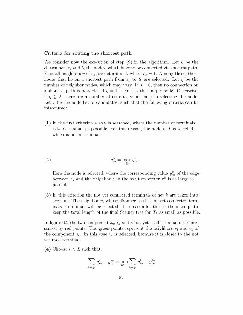
(1) In the first criterion a way is searched, where the number of terminalsis kept as small as possible. For this reason, the node in L is selectedwhich is not a terminal.

(2) yksv = max

u∈Lyksu

Here the node is selected, where the corresponding value yksv of the edge

between sk and the neighbor v in the solution vector yk is as large aspossible.

(3) In this criterion the not yet connected terminals of net k are taken intoaccount. The neighbor v , whose distance to the not yet connected term-inals is minimal, will be selected. The reason for this, is the attempt tokeep the total length of the final Steiner tree for Tk as small as possible.

In figure 6.2 the two component sk , tk and a not yet used terminal are repre-sented by red points. The green points represent the neighbors v1 and v2 ofthe component sk . In this case v2 is selected, because it is closer to the notyet used terminal.

(4) Choose v ∈ L such that:∑k 6=k0

yksv − yk0

sv = minu∈L

∑k 6=k0

yksu − yk0

su

52

Figure 6.2: An example for criterion 3

With criterion (4), an attempt is made to avoid those edges that are lik-ely to be preferred by another net.

(5) In the last criterion the node is selected, which gives less change in thedirection.

Figure 6.3: An example for criterion 5

53

In figure 6.3 an example for criterion (5) is sketched. In this case the neighborv2 will be selected, because in this case there would be no change of directionwith respect to the last connection.

In the selection of the node v it is proceeded as follows. First, the firstcriterion is examined. If the minimum is uniquely determined, so let v bethe corresponding node. If the minimum is not uniquely determined, allnodes that take the minimum in (1) will be used in criterion (2). If amongthese nodes the minimum in (2) is uniquely determined, then v is the cor-responding node. Otherwise, the process continues according to the criteria(3) to (5). If in criterion (5) no node is uniquely determined, any node v isselected. After every iteration from (1) to (5) a node is determined, whichis adjacent to s . Then the edge sv is added to the way W , set s = v anditerate until s = tk or no neighbor node, which is located on a shortest path(η = 0), was found.

6.1.4 Results

In principle, the cutting plane algorithm can be used to find an optimalsolution for the given switchbox routing problem or to determine that nosolution exists. However, this may often not be guaranteed in an acceptablecomputing time. Therefore Grotschel et al. [GMW96a] has integrated a timebarrier. If this time barrier is exceeded the process ends and gives out theuntil then best lower bound and the best feasible solution.

Grotschel et al. has given various results of different test examples. Theseswitchbox examples have often been discussed in the literature. They in-clude various difficulties, such as a very high density of the networks or aterminal intensive example, where all vertices of the outer face are terminals.The example difficult switchbox can be found in [BP83]. Examples terminalintensive switchbox, dense switchbox and augmented dense switchbox wereintroduced in [Luk85]. Finally, the examples modified dense switchbox, ped-agogical switchbox and more difficult switchbox can be found in [Coh88].

In table 6.1 it is shown how large the test examples are and how large theircorresponding nets are. In column 1 the name of the examples is listed. The

54

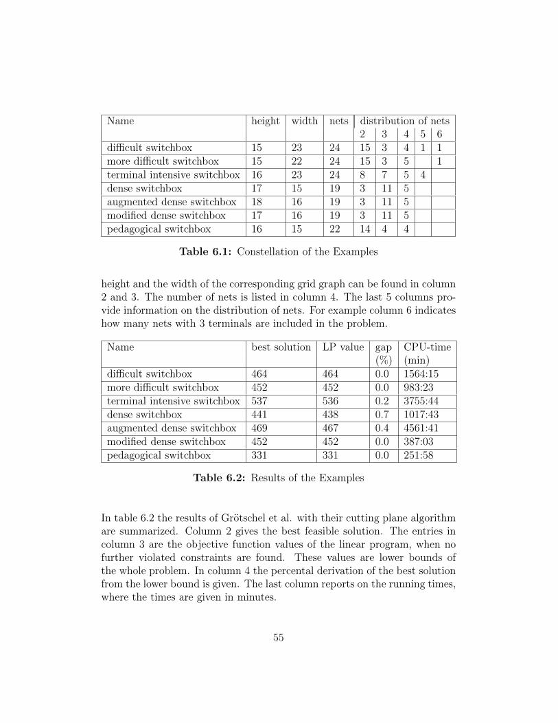
Name height width nets distribution of nets2 3 4 5 6

difficult switchbox 15 23 24 15 3 4 1 1more difficult switchbox 15 22 24 15 3 5 1terminal intensive switchbox 16 23 24 8 7 5 4dense switchbox 17 15 19 3 11 5augmented dense switchbox 18 16 19 3 11 5modified dense switchbox 17 16 19 3 11 5pedagogical switchbox 16 15 22 14 4 4

Table 6.1: Constellation of the Examples

height and the width of the corresponding grid graph can be found in column2 and 3. The number of nets is listed in column 4. The last 5 columns pro-vide information on the distribution of nets. For example column 6 indicateshow many nets with 3 terminals are included in the problem.

Name best solution LP value gap CPU-time(%) (min)

difficult switchbox 464 464 0.0 1564:15more difficult switchbox 452 452 0.0 983:23terminal intensive switchbox 537 536 0.2 3755:44dense switchbox 441 438 0.7 1017:43augmented dense switchbox 469 467 0.4 4561:41modified dense switchbox 452 452 0.0 387:03pedagogical switchbox 331 331 0.0 251:58

Table 6.2: Results of the Examples

In table 6.2 the results of Grotschel et al. with their cutting plane algorithmare summarized. Column 2 gives the best feasible solution. The entries incolumn 3 are the objective function values of the linear program, when nofurther violated constraints are found. These values are lower bounds ofthe whole problem. In column 4 the percental derivation of the best solutionfrom the lower bound is given. The last column reports on the running times,where the times are given in minutes.

55

The results are promising, such that for the given examples the best fea-sible solution deviates at most 0.7% from the optimal solution. Generally forproblem instances arising in VLSI-Design there is only given a heuristic. Theadvantage of the cutting plane algorithm is, that the quality of the heuristi-cally determined solution can be evaluated with the lower bound, which mayinclude knowledge about the problem itself.

This approach has been shown to be quite promising, but there are stillmany open problems that need to be solved. In order to solve large scaleproblem instances as they occur in practice, the algorithm must be improved.

56

Chapter 7

Implementation

The explained heuristic in chapter 6.1.3 has been implemented in Matlab.Given that this is a LP -based heuristic, various changes have been made,such that at least the main idea was implemented. Instead of using thesolution vector y , which is computed from a linear program, all values of yare set to 0. In general it can be said, that this simplification makes theheuristic independent of a linear program, such that it can be implementedwithin a Matlab environment.

7.1 The Algorithm

Each terminal of a net is considered as a component. Now iteratively alwaysjust two components of the same net will be connected. In which order thecomponents are connected, is depending on a function fk , which is explainedlater. The selected components have to be connected on a shortest path,where some criteria are important in order to limit the choices. If it is notpossible to connect the two components, then another pair of componentshave to be connected. Is there no possible way to connect two componentsvia shortest path, there should be a path via detour. If this is the case,there is no guarantee that the solution is optimal. The graph and all rele-vant datastructures will be updated and it will be continued with the nextiteration. This precedure will be iterated either until all nets are connectedor no more connections are possible. If it is not possible to connect two

57

components somehow, then the procedure will be interrupted, such that nosolution was found. In the following a detailed description of the algorithmis given:

Input:A complete rectangular rows × columns grid graph G = (V ,E ) withedge capacities ce = 1 and e ∈ E . Furthermore, a list of terminal setsN = {T1, ...,TN}.

Output:A feasible solution of the Steiner tree packing problem, given by theedge sets (S1, ..., SN ) or the message “No feasible solution found”.

(1) Set Sk := ∅ and the not yet used terminals T ′k = Tk for

k = 1, ...,N , and the graph G = G .(2) For k = 1, ...,N perform the following steps:(3) If Sk = ∅, then

determine sk , tk ∈ Tk such thatfk(sk , tk) = min

s,t∈Tks 6=t

fk(s , t);

set T ′k := Tk\{sk , tk}.(4) Else

determine sk ∈ T ′k , tk ∈ V (Sk) such thatfk(sk , tk) = min

s∈T ′k

t∈V (Sk )

fk(s , t)

(5) Try to connect sk with tk via a shortest path by taking thecriteria into account.

(6) If the connection via a shortest path is possible, then go to (9);(7) Else determine another pair (sk , tk), go to (3);(8) If the connection via a detour is possible, then(9) Update datastructures:

let W be the edge set of the chosen path;set Sk := Sk ∪W , T ′k := T ′k\{sk};delete all e ∈W from the graph G ;

(10) Else print the message “No feasible solution found”.(11) If all terminal sets are connected, return the feasible solution

(S1, ..., SN ).(12) STOP.

58

fk := |w(W (sk , tk))|

The function fyk presented in chapter 6 was changed to fk and is also used tofind the two components which have to be connected. The two componentsare searched, which have the smallest value resulting from the function. Thefunction gives the weighted sum of the shortest path from sk to tk .

For routing the shortest path, those criteria were taken, which have no re-lation to the solution vector y . The criteria (1), (3) and (5) from chapter 6were implemented.

7.2 Code

The implementation was programmed with Matlab, which is a high perfor-mance language for technical computing. It integrates computation, visu-alization, and programming in an easy-to-use environment, where problemsand solutions are expressed in familiar mathematical notation.

Given that this is a graph-theoretic problem, it turned out to be usefull touse a toolbox. MATGRAPH is a toolbox provided by Scheinerman [Sch08]for working with simple graphs in Matlab. The goal of this toolbox was, tomake interactive graph theory exploration simple and efficient.

In figure 7.1 a grid graph is shown, which was created with MATGRAPH.In order to understand the calculations in the following functions of the al-gorithm, it is intended to show how the vertices are arranged. The verticesare labeled with their corresponding number.

59

Figure 7.1: Structure of a grid graph

Similarly as in chapter 6.1.3 the minimum enclosing rectangle was used, buthere in a differnt way. A shortest path between two vertices must run withintheir minimum enclosing rectangle. If there is no possible connection insidethis rectangle, then there should be a connection via detour. Otherwise nopath between the two vertices is available. In the following some functionsare presented, where the minimal enclosing rectangle is abbreviated with mer.

The function merVertices determines all vertices of the minimal enclosingrectangle between the two vertices u and v . Additionally the height and thewidth are determined.

function [vert ,h,w] = merVertices(rows ,columns ,u,v)

%determine height

h_u = mod(u-1,rows)+1;

h_v = mod(v-1,rows)+1;

h = abs(h_u -h_v)+1;

60

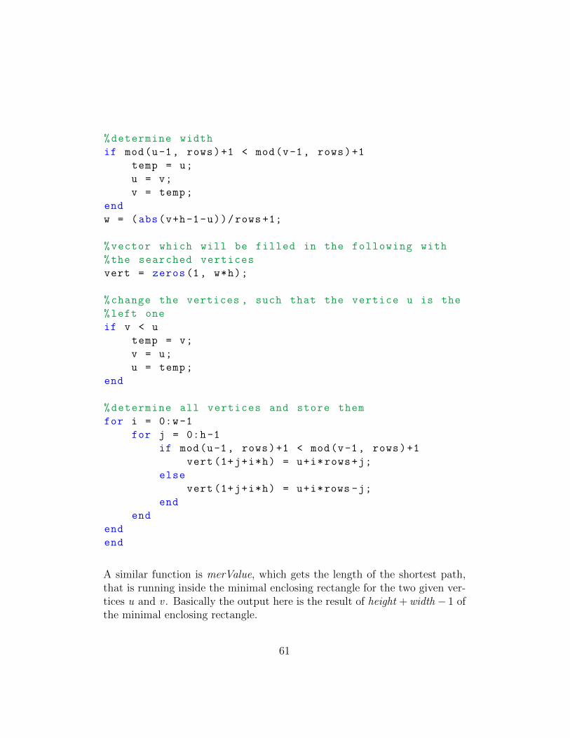
%determine width

if mod(u-1, rows)+1 < mod(v-1, rows)+1

temp = u;

u = v;

v = temp;

end

w = (abs(v+h-1-u))/rows +1;

%vector which will be filled in the following with

%the searched vertices

vert = zeros(1, w*h);

%change the vertices , such that the vertice u is the

%left one

if v < u

temp = v;

v = u;

u = temp;

end

%determine all vertices and store them

for i = 0:w-1

for j = 0:h-1

if mod(u-1, rows)+1 < mod(v-1, rows)+1

vert (1+j+i*h) = u+i*rows+j;

else

vert (1+j+i*h) = u+i*rows -j;

end

end

end

end

A similar function is merValue, which gets the length of the shortest path,that is running inside the minimal enclosing rectangle for the two given ver-tices u and v . Basically the output here is the result of height + width − 1 ofthe minimal enclosing rectangle.

61

The function merMin finds the one vertex from each vertex set T 1 andT 2, which have to be connected. In general the two vertices are searched,where the length of the shortest path is minimal. This function plays animportant role in the steps (3) and (4) of the algorithm.

function [a, b] = merMin(g, rows , columns , T1, T2)

%declaration

a = 0; %index of the first vertice in T1

b = 0; %index of the second vertice in T2

value = rows * columns; %biggest possible value

%save the the two vertices with the minimal

%shortest path

for i = 1:size(T1, 2) -1

for j = i+1: size(T2, 2)

if merValue(g, rows , columns , T1(i), T2(j))

< value

value = merValue(g, rows , columns , T1(i),

T2(j));

a = i;

b = j;

end

end

end

end

In step (3) the vertice sets T 1 and T 2 are equal the terminal set Tk . Howeverin step (4) T 1 is the set of the not yet connected terminals T ′k and T 2 is theset of vertices V (Sk).

The function merShortestPath determines every shortest path from verticeu to v . In addition there are some criteria, such that the path which satisfyall the criteria, will be chosen. This function is used for step (5) of the algo-rithm. It is first checked, if the given vertices are valid, which means that thevertices exists in the graph G and that they are not equal. Then all neighbor

62

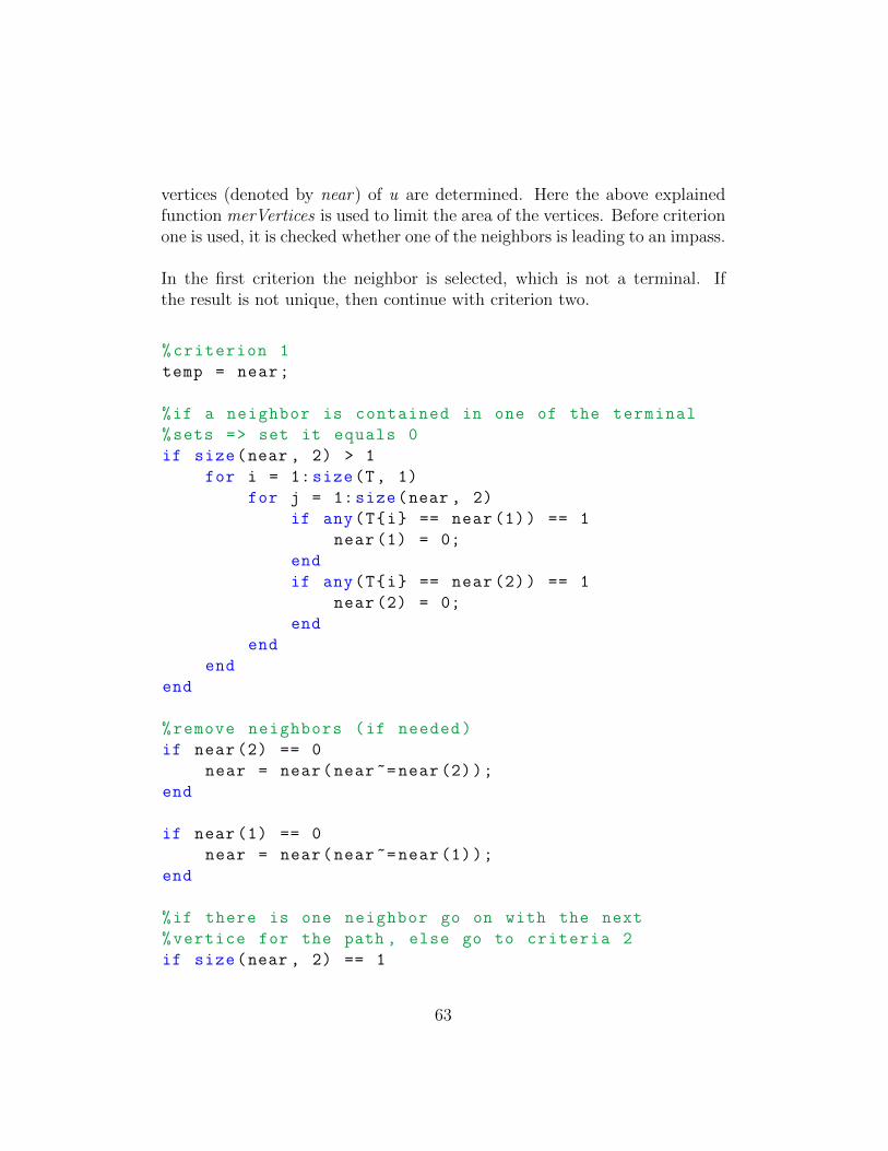
vertices (denoted by near) of u are determined. Here the above explainedfunction merVertices is used to limit the area of the vertices. Before criterionone is used, it is checked whether one of the neighbors is leading to an impass.

In the first criterion the neighbor is selected, which is not a terminal. Ifthe result is not unique, then continue with criterion two.

%criterion 1

temp = near;

%if a neighbor is contained in one of the terminal

%sets => set it equals 0

if size(near , 2) > 1

for i = 1:size(T, 1)

for j = 1:size(near , 2)

if any(T{i} == near (1)) == 1

near (1) = 0;

end

if any(T{i} == near (2)) == 1

near (2) = 0;

end

end

end

end

%remove neighbors (if needed)

if near (2) == 0

near = near(near~=near (2));

end

if near (1) == 0

near = near(near~=near (1));

end

%if there is one neighbor go on with the next

%vertice for the path , else go to criteria 2

if size(near , 2) == 1

63

path = [path near (1)];

continue;

else

near = temp;

end

In the second criterion the not yet connected terminals of the same net aretaken into account. The function shortestPath determines every shortestpath from vertice u and v to all vertices in set T ′.

%criterion 2

function direction = shortestPath(g, start , u, v, T)

%Output: 0 => the length of the paths are equal

% 1 => u is the chosen vertex

% 2 => v is the chosen vertex

length_u = size(edges(g), 1);

length_v = size(edges(g), 1);

direction = 0;

T = T(T~= start);

%determine all shortest paths to the not yet

%connected terminals and store the smallest one

for i=1: size(T, 2)

path = find_path(g, u, T(i));

if length_u > size(path , 2)

length_u = size(path , 2);

end

path = find_path(g, v, T(i));

if length_v > size(path , 2)

length_v = size(path , 2);

end

end

if length_u < length_v

direction = 1;

64

end

if length_v < length_u

direction = 2;

end

end

The vertex with the shortest path will be the chosen one. The output is 1,if u is the chosen vertex and 2 if v is the chosen vertex. Otherwise if theselengths are equal, then the output is 0, in this case continue with criterion 3.

In the last criterion the node is selected, which gives less change in thedirection as explained in section 6.1.3. The vector path contains the untilthen determined shortest path.

%criterion 3

if size(path , 2) >= 2

if abs(path(end)-path(end -1)) == rows

if path(end) < last

path = [path near (2)];

else

path = [path near (1)];

end

continue;

end

if abs(path(end)-path(end -1)) == 1

if path(end) < last

path = [path near (1)];

else

path = [path near (2)];

end

continue;

end

end

If no connection via the shortest path within the minimum enclosing rect-angle is possible, then there must be a detour. The function findDetourdetermines a path, which is as small as possible, that connects two compo-

65

nents. Finally, the following heuristic was created by using the presentedfunctions.

function [S] = heuristic(example_name)

%% Input

struct = importdata(example_name);

T = getfield(struct , ’S’); %terminal sets

c = getfield(struct , ’c’); %columns

r = getfield(struct , ’r’); %rows

dim = getfield(struct , ’dim’); %span

%% Initialization

graph_init;

G = graph;

grid(G,r,c); %grid graph

k = size(T,1); %number of terminal sets

S = cell(k,1); %egde sets for the Steiner trees

VS = cell(k,1); %all vertices of each Steiner tree

T_ = T; %terminals which are not used

%% Algorithm

for j=1: dim

for i=1:k

path = [];

if isempty(S{i}) %if edge set i is empty

temp = T_{i};

while isempty(path) && size(temp ,2) >= 2

[s_k ,t_k] = merMin(G, r, c, temp , temp);

path = merShortestPath(G, r, c, i, temp(

s_k), temp(t_k), T, T_);

if isempty(path)

temp([t_k]) = [];

end

end

if isempty(path)

temp = T_{i};

66

[s_k , t_k , path] = findDetour(G, r, c,

T_{i}, T_{i});

end

if s_k ~= 0

VS{i} = [VS{i} path];

T_{i} = T_{i}(T_{i}~= temp(s_k));

T_{i} = T_{i}(T_{i}~= temp(t_k));

else

’No solution found’

return;

end

else %if terminal set i is not empty

if ~isempty(T_{i})

temp = T_{i};

while isempty(path) && size(temp ,2) >= 2

[s_k , t_k] = merMin(G, r, c, temp , VS{i

});

path = merShortestPath(G, r, c, i, temp(

s_k), VS{i}(t_k), T, T_);

if isempty(path)

temp([s_k]) = [];

end

end

if isempty(path)

temp = T_{i};

[s_k , t_k , path] = findDetour(G, r, c,

T_{i}, VS{i});

end

if s_k ~= 0

VS{i} = [VS{i} path (1: size(path ,2) -1)];

T_{i} = T_{i}(T_{i}~= temp(s_k));

else

’No solution found’

return;

end

end

end

%save used edges and delete them from the graph

67

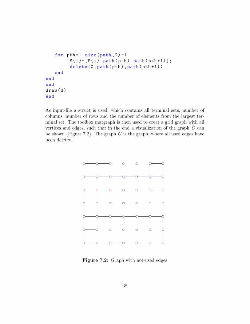
for pth=1: size(path ,2) -1

S{i}=[S{i} path(pth) path(pth+1)];

delete(G,path(pth),path(pth+1))

end

end

end

draw(G)

end

As input-file a struct is used, which contains all terminal sets, number ofcolumns, number of rows and the number of elements from the largest ter-minal set. The toolbox matgraph is then used to creat a grid graph with allvertices and edges, such that in the end a visualization of the graph G canbe shown (Figure 7.2). The graph G is the graph, where all used edges havebeen deleted.

Figure 7.2: Graph with not-used edges

68

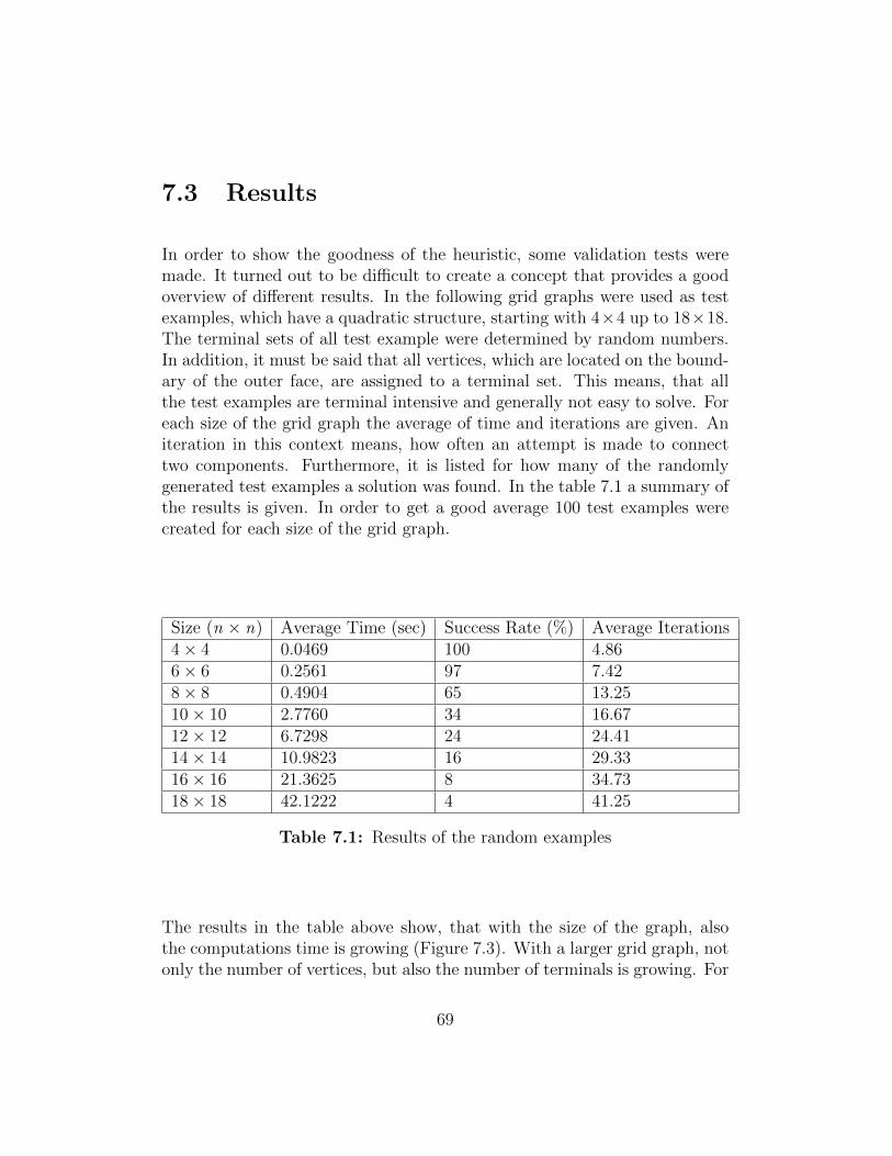
7.3 Results

In order to show the goodness of the heuristic, some validation tests weremade. It turned out to be difficult to create a concept that provides a goodoverview of different results. In the following grid graphs were used as testexamples, which have a quadratic structure, starting with 4×4 up to 18×18.The terminal sets of all test example were determined by random numbers.In addition, it must be said that all vertices, which are located on the bound-ary of the outer face, are assigned to a terminal set. This means, that allthe test examples are terminal intensive and generally not easy to solve. Foreach size of the grid graph the average of time and iterations are given. Aniteration in this context means, how often an attempt is made to connecttwo components. Furthermore, it is listed for how many of the randomlygenerated test examples a solution was found. In the table 7.1 a summary ofthe results is given. In order to get a good average 100 test examples werecreated for each size of the grid graph.

Size (n × n) Average Time (sec) Success Rate (%) Average Iterations4× 4 0.0469 100 4.866× 6 0.2561 97 7.428× 8 0.4904 65 13.2510× 10 2.7760 34 16.6712× 12 6.7298 24 24.4114× 14 10.9823 16 29.3316× 16 21.3625 8 34.7318× 18 42.1222 4 41.25

Table 7.1: Results of the random examples

The results in the table above show, that with the size of the graph, alsothe computations time is growing (Figure 7.3). With a larger grid graph, notonly the number of vertices, but also the number of terminals is growing. For

69

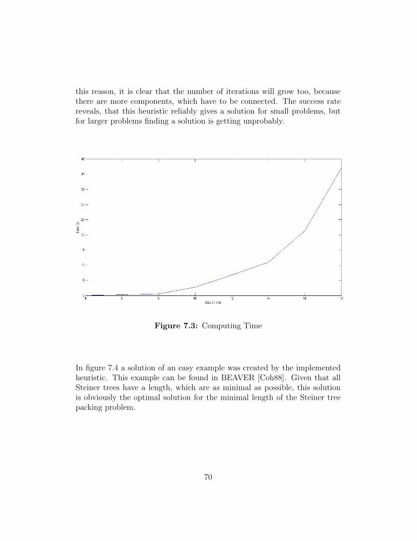
this reason, it is clear that the number of iterations will grow too, becausethere are more components, which have to be connected. The success ratereveals, that this heuristic reliably gives a solution for small problems, butfor larger problems finding a solution is getting unprobably.

Figure 7.3: Computing Time

In figure 7.4 a solution of an easy example was created by the implementedheuristic. This example can be found in BEAVER [Coh88]. Given that allSteiner trees have a length, which are as minimal as possible, this solutionis obviously the optimal solution for the minimal length of the Steiner treepacking problem.

70

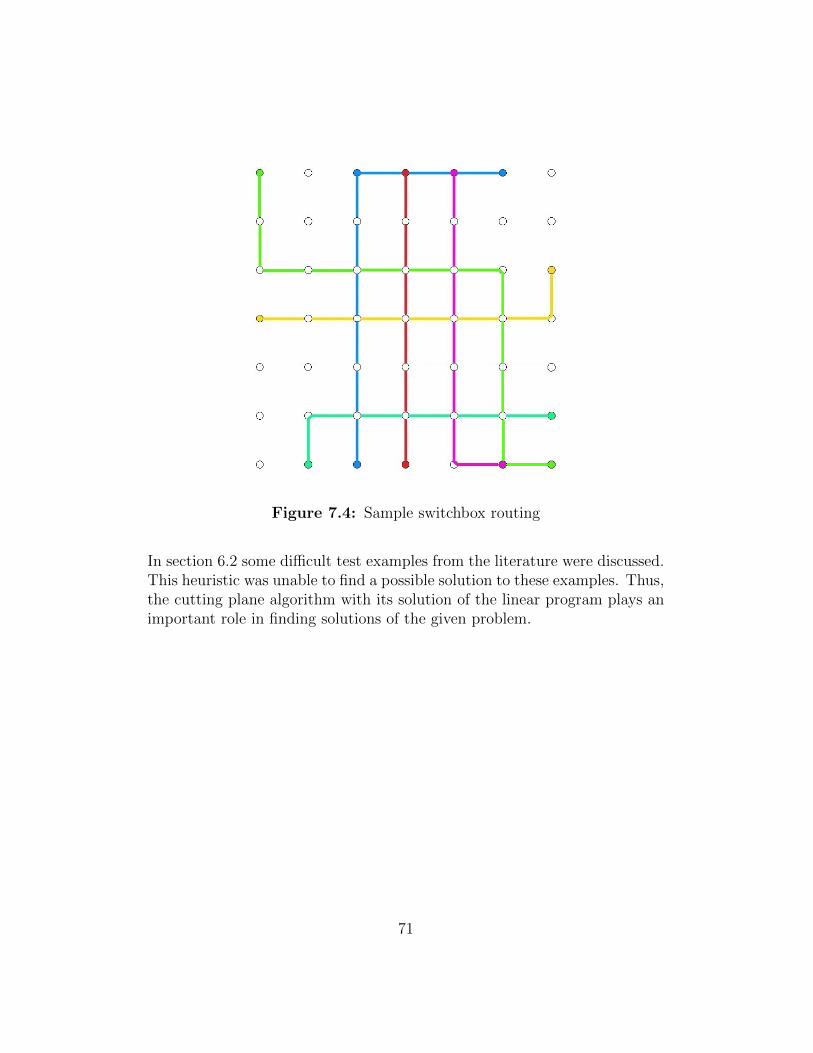
Figure 7.4: Sample switchbox routing

In section 6.2 some difficult test examples from the literature were discussed.This heuristic was unable to find a possible solution to these examples. Thus,the cutting plane algorithm with its solution of the linear program plays animportant role in finding solutions of the given problem.

71

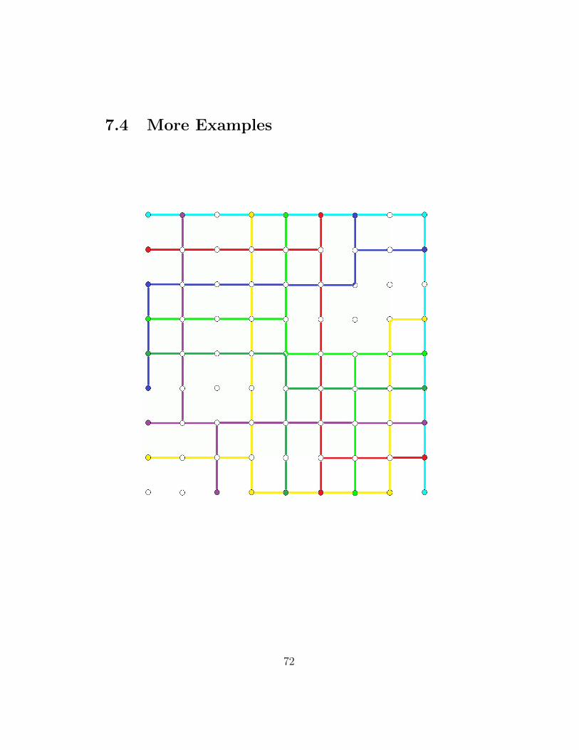
7.4 More Examples

72

73

Chapter 8

Conclusion

In this thesis the problem of packing Steiner trees is considered. It is givenan extensive background knowledge of this problem, for example definitionsof the graph theory, linear programming and of the underlying Steiner treeproblem. Furthermore, there are given some related problems from the lit-erature and the main application of the Steiner tree packing problem, theVLSI-Design, is studied. An important subproblem that occurs in the VLSI-Design, can be solved by using the Steiner tree packing problem. Somedetailed routing models, which can be derived from there, are also presented.In the thesis the switchbox routing model was discussed in more detail.

A survey of different integer programming models, which solve the Steinertree packing problem, is given. It focuses on computational aspects of theproblem. The undirected cut formulation is used in the cutting plane algo-rithm to solve the switchbox routing problem in the knock-knee model. Forthis the inter program had to be relaxed, such that each variable belong tothe interval [0, 1], which is called an linear programming relaxation. Thecutting plane algorithm uses the computed solutions of the linear programand tries to find a feasible solution with a heuristic. It came out, that thisapproach finds either an optimal solition, or at least a lower bound of theproblem.

This approach has been shown to be quite promising, but there are stillopen problems, that need to be solved like seperation methods, where noexact algorithm is provided. With the results, which were presented in thisthesis, it can be hoped that the approach can also be used for solving prob-

74

lems of practical examples. In order to solve large scale problem instances asthey occur in practice, the algorithm must be improved. For example, by re-ducing the computation time with a smaller number of variables in the linearprogram. This can possibly reached by reducing the area for each terminalset in the minimal enclosing area.

The heuristic of the presented approach has been implemented in Matlab,but with a symplification, that made the heuristic independent of a linearprogram. This heuristic turned out to be significantly worse than the cuttingplane algorithm. Consequently, it can be said, that the linear program playsa very important role of finding solutions for the Steiner tree packing prob-lem in the approach. This algorithm behaves much faster, but for a growingsize of the graph, the success rate is running pretty fast towards zero.

75

Bibliography

[Aaz08] Aazami, Ashkan: Hardness results and approximation algo-rithms for some problems on graphs. (2008)

[APD03] Althaus, Ernst ; Polzin, Tobias ; Daneshmand, Siavash Vah-dati: Improving Linear Programming Approaches for the SteinerTree Problem. In: Experimental and Efficient Algorithms: Lec-ture Notes in Computer Science, Volume 2647, pp 1-14 (2003)

[BB84] Brady, M.L. ; Brown, D.J.: VLSI routing: Four layers suffice.Advances in Computing Research, Volume 2, pp 245-258, (1984)

[BB00] Bienstock, D. ; Bley, A.: Capacitated Network Design withMulticast Commodities. In: International Conference Telecom-munication Systems, pp 575-599 (2000)

[Bix91] Bixby, Robert E.: Implementing The Simplex Method: TheInitial Basis. In: Rice University: Department of MathematicalSciences (1991)

[BM08] Bondy, J.A. ; Murty, U.S.R.: Graph Theory. Graduate Textsin Mathematics, Volume 244, (2008)

[BP83] Burstein, M. ; Pelavin, R.: Hierachical wire routing.In: IEEE Transactions on Computer-Aided-Design, pp 223-234(1983)

[Cho94] Chopra, Sunil: Comparison of formulations and a heuristicfor packing Steiner trees in a graph. In: Annals of OperationsResearch 50, pp 143-171 (1994)

76

[Coh88] Cohoon, J. P.: BEAVER: computational geometry-based toolfor switchbox routing. In: IEEE Transactions on Computer-Aided-Design CAD-7, pp 684-697 (1988)

[Edm65] Edmonds, J.: Minimum partition of a matroid into independentsubsets. In: Journal of Research National Bureau of StandardsSections B, pp 67-72 (1965)

[FKK03] Frank, A. ; Kiraly, T. ; Kriessel, M.: On decomposinga hypergraph into k connected sub-hypergraphs. In: DiscreteApplied Methematics, Volume 131, pp 373-383 (2003)

[GJ77] Garey, M.R. ; Johnson, D.S.: The rectilinear Steiner treeproblem is NP -complete. In: SIAM Journal on Applied Mathe-matics 32, pp 835-859 (1977)

[GMW93] Grotschel, M. ; Martin, A. ; Weismantel, R.: PackingSteiner Trees: seperation algorithms. In: Konrad-Zuse-Zentrumfur Informationstechnik Berlin, Preprint SC 93-2 (1993)

[GMW96a] Grotschel, M. ; Martin, A. ; Weismantel, R.: PackingSteiner Trees: A Cutting Plane Algorithm and ComputationalResults. In: Mathematical Programming, Volume 72, pp 125-145(1996)

[GMW96b] Grotschel, M. ; Martin, A. ; Weismantel, R.: PackingSteiner Trees: Further Facets. In: Europ. J. Combinatorics,Volume 17, pp 39-52 (1996)

[GMW97] Grotschel, M. ; Martin, A. ; Weismantel, R.: The SteinerTree Packing Problem in VLSI-Design. In: Mathematical Pro-gramming, Volume 78, pp 265-281 (1997)

[Gol10] Goldreich, Oded: P, NP, and NP-Completeness: The Ba-sics of Computational Complexity. Cambridge University Press,(2010)

[Hak71] Hakimi, S.L.: Steiner’s problem in graphs and its implications.In: Networks 1, pp 113-133 (1971)

77

[HRW92] Hwang, Frank K. ; Richards, Dana S. ; Winter, Pawel: TheSteiner Tree Problem. Annals of Descrete Mathematics, Volume53, 1992

[JLPP02] Jeong, Gue-woong ; Lee, Kyungsik ; Park, Sungsoo ; Park,Kyungchul: A branch-and-price algorithm for the Steiner treepacking problem. In: Computer & Operations Research 29, pp221-241 (2002)

[JMS03] Jain, K. ; Mahdian, M. ; Salvatipour, M.R.: Packing Steinertrees. In: Proceedings of the fourteenth annual ACM-SIAM sym-posium on Discrete algorithms, pp 266-274 (2003)

[Kar10] Karp, R.M.: Reducibility among combinatorial problems. In:50 Years of Integer Programming 1958-2008, pp 219-241 (2010)

[KH12] Koch, Thorsten ; Hoang, Nam-Du.: Steiner tree packing revis-ited. In: Mathematical Methods of Operations Research, Volume76, pp 95-123 (2012)

[KPS90] Korte, B. ; Promel, H.J. ; Schrijver, A.: Steiner trees inVLSI-layout. In: Paths, Flows, and VLSI-Layout, pp 185-214(1990)

[Kv80] Kramer, M.R. ; van Leeuwen, J.: The complexity of wire-routing and finding minimum area layouts for arbitrary VLSIcircuits. In: Advances in Computing Research 2, pp 270-281(1980)

[Lau07] Lau, Lap C.: An Approximate Max-Steiner-Tree-Packing Min-Steiner-Cut Theorem. In: Combinatorica, Volume 27, pp 71-90(2007)

[Len90] Lengauer, T.: Combinatorial Algorithms for Integrated CircuitLayout. John Wiley & Sons, (1990)

[Lev71] Levin, A.Y.: Algorithm for shortest connection of a group ofgraph vertices. In: Sov. Math. Dokl., Volume 12, pp 1477-1481(1971)

78

[LL93] Lengauer, T. ; Lugering, M.: Integer programming formu-lations of global routing and placement problems. In: ResearchReport, University of Paderborn (1993)

[LS91] Liao, Kuo-Feng ; Sarrafzadeh, Majid: Vertex-disjoint treesand boundary single-layer routing. In: Graph-Theoretic Con-cepts in Computer Science: Lecture Notes in Computer Science,Volume 484, pp 99-108 (1991)

[Luk85] Luk, W. K.: A greedy switch-box router. In: Integration, Vol-ume 3, pp 129-149 (1985)

[Mel61] Melzak, Z.A.: On the problem of Steiner. In: Canadian Math-ematical Bulletin, Volume 4, pp 143-148 (1961)

[MG07] Matousek, Jir ; Grtner, Bernd: Integer Programming andLP Relaxation. In: Understanding and Using Linear Program-ming Universitext, pp 29-40 (2007)

[MP93] Middendorf, M. ; Pfeiffer, F.: On the complexity of thedisjoint paths problem. In: Combinatorica, Volume 13, pp 185-107 (1993)

[NS08] Naves, G. ; Sebo, A.: Multifow feasibility: an annotatedtableau. In: Research Trends in Combinatorial Optimization,pp 261-283 (2008)

[RRSS93] Reed, B. ; Robertson, N. ; Schrijver, A. ; Seymour, P.D.:Finding disjoint trees in graphs on surfaces. (1993)

[RS90] Robertson, N. ; Seymour, P.D.: An outline of a disjointpaths algorithm. In: Path, Flows and Vlsi-Layout (1990)

[RT87] Raghavan, P. ; Thompson, C.D.: Randomized rounding: Atechnique for provably good algorithms and algorithmic proofs.In: Combinatorica, Volume 7, pp 365-374 (1987)

[Ruo13] Ruohonen, Keijo: Graph Theory. Tampere University of Tech-nology, (2013)

79

[Sar87] Sarrafzadeh, M.: Channel-routing problem in the knock-kneemode is NP -complete. In: IEEE Transactions on Computer-Aided-Design CAD-6, pp 503-506 (1987)

[Sch08] Scheinerman, Edward R.: MATGRAPH: A Matlab ToolboxFor Graph Theory. In: Department of Applied MathematicsStatistics Vice Dean for Education, Whiting School of Engineer-ing Johns Hopkins University (2008)

[Str10] Streck, Stefanie: The Fermat problem. In: Pacific LutheranUniversity (2010)

[Van08] Vanderbei, Robert J.: Linear Programming. InternationalSeries in Operations Research & Management Science, Volume114, (2008)

[Won84] Wong, R.T.: A dual approach for the steiner tree on a directedgraph. In: Mathematical Programming 28, pp 271-287 (1984)

80