models, methods and tools for bridging the design
TRANSCRIPT

HAL Id: tel-01610096https://tel.archives-ouvertes.fr/tel-01610096
Submitted on 5 Oct 2017
HAL is a multi-disciplinary open accessarchive for the deposit and dissemination of sci-entific research documents, whether they are pub-lished or not. The documents may come fromteaching and research institutions in France orabroad, or from public or private research centers.
L’archive ouverte pluridisciplinaire HAL, estdestinée au dépôt et à la diffusion de documentsscientifiques de niveau recherche, publiés ou non,émanant des établissements d’enseignement et derecherche français ou étrangers, des laboratoirespublics ou privés.
Models, Methods and Tools for Bridging the DesignProductivity Gap of Embedded Signal Processing
SystemsMaxime Pelcat
To cite this version:Maxime Pelcat. Models, Methods and Tools for Bridging the Design Productivity Gap of EmbeddedSignal Processing Systems. Signal and Image processing. Université Clermont Auvergne, 2017. �tel-01610096�

M A X I M E P E L C AT
M O D E L S , M E T H O D S A N D T O O L S
F O R B R I D G I N G T H E D E S I G N
P R O D U C T I V I T Y G A P O F
E M B E D D E D S I G N A L P R O C E S S I N G
S Y S T E M S
Soutenue le 10 ju i l l e t 2017 devan t un ju ry composé de
RAPPORTEURS :
M I C H E L A U G U I N, D R C N R SJ E A N - P I E R R E TA L P I N , D R I N R I AC H R I S T O P H E J É G O , P R O F. E N S E I R B - M AT M E C AEXAM I NAT EURS :
J O C E LY N S É R O T, P R O F. U C AF R A N Ç O I S B E R R Y, M C F H D R U C AJ E A N - F R A N Ç O I S N E Z A N , P R O F. I N S A R E N N E S / I E T RD A N I E L M É N A R D, P R O F. I N S A R E N N E S / I E T RS H U V R A S . B H AT TA C H A R Y YA , P R O F. U M D / T U T
H A B I L I TAT I O N À D I R I G E R D E S R E C H E R C H E S


Contents
List of Personal Publications 5
Foreword 9
Abstract 11
1 Design Productivity 13
A Using Dataflow MoCs for Raising Design Productivity 19
2 Improving Design Efficiency 21
3 Improving Implementation Quality 41
4 Evaluating Design Productivity 51
B Introducing MoAs for Raising Design Productivity 71
5 Models of Architecture: A New Design Abstraction 73
6 State of the Art of Models of Architecture 85
7 Models of Architecture in Practice 105
8 Research Perspectives 121
Bibliography 129


List of Personal Publications
[1] Carlo Sau, Francesca Palumbo, Maxime Pelcat, Julien Heulot, Erwan Nogues, Daniel Ménard, Paolo Meloni,
and Luigi Raffo. Challenging the best HEVC fractional pixel FPGA interpolators with reconfigurable and multi-
frequency approximate computing. IEEE Embedded Systems Letters, 2017. IEEE, to appear.
[2] Alexandre Mercat, Florian Arrestier, Wassim Hamidouche, Maxime Pelcat, and Daniel Menard. Energy reduction
opportunities in an HEVC real-time encoder. In Proceedings of the ICASSP conference. IEEE, 2017.
[3] Alexandre Mercat, Florian Arrestier, Wassim Hamidouche, Maxime Pelcat, and Daniel Menard. Constrain the
docile CTUs: an in-frame complexity allocator for HEVC intra encoders. In Proceedings of the ICASSP conference.
IEEE, 2017.
[4] Michael Masin, Francesca Palumbo, Hans Myrhaug, Julio de Oliveira Filho, Max Pastena, Maxime Pelcat, Luigi
Raffo, Francesco Regazzoni, Angel Sanchez, Antonella Toffetti, Eduardo de la Torre, and Katiuscia Zedda. Cross-
layer design of reconfigurable cyber-physical systems. In Proceedings of the DATE Conference. IEEE ACM, 2017.
[5] Erwan Raffin, Wassim Hamidouche, Erwan Nogues, Maxime Pelcat, and Daniel Menard. Scalable HEVC De-
coder for Mobile Devices: Trade-offs between Energy Consumption and Quality. In Proceedings of the DASIP
conference. IEEE, 2016.
[6] Alexandre Mercat, Wassim Hamidouche, Maxime Pelcat, and Daniel Menard. Estimating encoding complexity of
a real-time embedded software hevc codec. In Proceedings of the DASIP conference. IEEE, 2016.
[7] Raquel Lazcano, Daniel Madroñal, Karol Desnos, Maxime Pelcat, Raúl Guerra, Sebastián López, Eduardo Juarez,
and César Sanz. Parallelism Exploitation of a Dimensionality Reduction Algorithm Applied to Hyperspectral
Images. In Proceedings of the DASIP Conference. IEEE, 2016.
[8] Kamel Abdelouahab, Cédric Bourrasset, Maxime Pelcat, François Berry, Jean-Charles Quinton, and Jocelyn Serot.
A holistic approach for optimizing DSP block utilization of a CNN implementation on FPGA. In Proceedings of
the ICDSC Conference. ACM, 2016.
[9] Maxime Pelcat, Karol Desnos, Luca Maggiani, Yanzhou Liu, Julien Heulot, Jean-François Nezan, and Shuvra S.
Bhattacharyya. Models of Architecture: Reproducible Efficiency Evaluation for Signal Processing Systems. In
Proceedings of the SiPS Workshop. IEEE, 2016.
[10] Karol Desnos, Maxime Pelcat, Jean-François Nezan, and Slaheddine Aridhi. Distributed memory allocation tech-
nique for synchronous dataflow graphs. In Proceedings of the SiPS Workshop. IEEE, 2016.

6
[11] Francesca Palumbo, Carlo Sau, Davide Evangelista, Paolo Meloni, Maxime Pelcat, and Luigi Raffo. Runtime
Energy versus Quality Tuning in Motion Compensation Filters for HEVC. In Proceedings of PDeS. IEEE, 2016.
[12] Maxime Pelcat, Cédric Bourrasset, Luca Maggiani, and François Berry. Design productivity of a high level
synthesis compiler versus HDL. In Proceedings of the IC-SAMOS Workshop. IEEE, 2016.
[13] Erwan Nogues, Daniel Menard, and Maxime Pelcat. Algorithmic-level approximate computing applied to energy
efficient HEVC decoding. IEEE Transactions on Emerging Topics in Computing, 2016. IEEE.
[14] Erwan Nogues, Julien Heulot, Glenn Herrou, Ladislas Robin, Maxime Pelcat, Daniel Menard, Erwan Raffin,
and Wassim Hamidouche. Efficient DVFS for low power HEVC software decoder. Journal of Real-Time Image
Processing, 2016. Springer Verlag.
[15] John McAllister, Maire O’neill, and Maxime Pelcat. Guest editorial: New frontiers in signal processing applica-
tions and embedded processing technologies. Journal of VLSI Signal Processing Systems for Signal, Image, and
Video Technology (JSPS), 2016. Springer Verlag.
[16] Erwan Nogues, Maxime Pelcat, Daniel Menard, and Alexandre Mercat. Energy efficient scheduling of real time
signal processing applications through combined DVFS and DPM. In Proceedings of the PDP conference. IEEE,
2016.
[17] Manel Ammar, Mouna Baklouti, Maxime Pelcat, Karol Desnos, and Mohamed Abid. On Exploiting Energy-
Aware Scheduling Algorithms for MDE-Based Design Space Exploration of MP2SoC. In Proceedings of the PDP
Conference. IEEE, 2016.
[18] Miguel Chavarrias, Fernando Pescador, Matias Garrido, Maxime Pelcat, and Eduardo Juarez. Design of Multicore
HEVC Decoders Using Actor-based Dataflow Models and OpenMP. In Proceedings of the ICCE Conference.
IEEE, 2016.
[19] Karol Desnos, Maxime Pelcat, Jean François Nezan, and Slaheddine Aridhi. On Memory Reuse Between Inputs
and Outputs of Dataflow Actors. ACM Transactions on Embedded Computing Systems (TECS), 2016. ACM.
[20] Simon Holmbacka, Erwan Nogues, Maxime Pelcat, Sébastien Lafond, Daniel Menard, and Johan Lilius. Energy-
awareness and performance management with parallel dataflow applications. Journal of VLSI Signal Processing
Systems for Signal, Image, and Video Technology (JSPS), 2015. Springer Verlag.
[21] Erwan Raffin, Erwan Nogues, Wassim Hamidouche, Seppo Tomperi, Maxime Pelcat, and Daniel Menard. Low
power HEVC software decoder for mobile devices. Journal of Real-Time Image Processing, 2015. Springer Verlag.
[22] Erwan Nogues, Erwan Raffin, Maxime Pelcat, and Daniel Menard. A modified HEVC decoder for low power
decoding. In Proceedings of the Computing Frontiers Conference. ACM, 2015.
[23] Erwan Raffin, Wassim Hamidouche, Erwan Nogues, Maxime Pelcat, Daniel Menard, and Tomperi Seppo. En-
ergy Efficiency of a Parallel HEVC Software Decoder for Embedded Devices. In Proceedings of the Computing
Frontiers Conference. ACM, 2015.
[24] Karol Desnos, Maxime Pelcat, Jean-François Nezan, and Slaheddine Aridhi. Buffer Merging Technique for Min-
imizing Memory Footprints of Synchronous Dataflow Specifications. In Proceedings of the ICASSP Conference.
IEEE, 2015.

7
[25] Manel Ammar, Mouna Baklouti, Maxime Pelcat, Karol Desnos, and Mohamed Abid. Automatic generation
of S-LAM descriptions from UML/MARTE for the DSE of massively parallel embedded systems. In Software
Engineering, Artificial Intelligence, Networking and Parallel/Distributed Computing. 2015. Springer Verlag.
[26] Erwan Nogues, Berrada Romain, Maxime Pelcat, Daniel Menard, and Erwan Raffin. A DVFS based HEVC
decoder for energy-efficient software implementation on embedded processors. In Proceedings of the ICME con-
ference. IEEE, 2015.
[27] Karol Desnos, Maxime Pelcat, Jean-François Nezan, and Slaheddine Aridhi. Memory Analysis and Optimized
Allocation of Dataflow Applications on Shared-Memory MPSoCs. Journal of VLSI Signal Processing Systems for
Signal, Image, and Video Technology (JSPS), 2014. Springer Verlag.
[28] Julien Heulot, Maxime Pelcat, Jean-François Nezan, Yaset Oliva, Slaheddine Aridhi, and Shuvra S Bhattacharyya.
Just-in-time scheduling techniques for multicore signal processing systems. In Proceedings of the GlobalSIP con-
ference. IEEE, 2014.
[29] Karol Desnos, Safwan El Assad, Aurore Arlicot, Maxime Pelcat, and Daniel Menard. Efficient multicore imple-
mentation of an advanced generator of discrete chaotic sequences. In Proceedings of the ICITST conference. IEEE,
2014.
[30] Zheng Zhou, William Plishker, Shuvra S Bhattacharyya, Karol Desnos, Maxime Pelcat, and Jean-François Nezan.
Scheduling of parallelized synchronous dataflow actors for multicore signal processing. Journal of VLSI Signal
Processing Systems for Signal, Image, and Video Technology (JSPS), 2014. Springer Verlag.
[31] Julien Heulot, Maxime Pelcat, Karol Desnos, Jean François Nezan, Slaheddine Aridhi, et al. SPIDER: A syn-
chronous parameterized and interfaced dataflow-based RTOS for multicore DSPs. Proceedings of the EDERC
Conference, 2014.
[32] Manel Ammar, Mouna Baklouti, Maxime Pelcat, Karol Desnos, and Mohamed Abid. MARTE to πSDF transfor-
mation for data-intensive applications analysis. In Proceedings of the DASIP Conference. IEEE, 2014.
[33] Simon Holmbacka, Erwan Nogues, Maxime Pelcat, Sébastien Lafond, and Johan Lilius. Energy efficiency and
performance management of parallel dataflow applications. In Proceedings of the DASIP conference. IEEE, 2014.
[34] Erwan Nogues, Simon Holmbacka, Maxime Pelcat, Daniel Menard, and Johan Lilius. Power-aware HEVC de-
coding with tunable image quality. In Proceedings of the SiPS Workshop. IEEE, 2014.
[35] Maxime Pelcat, Karol Desnos, Julien Heulot, Clément Guy, Jean-François Nezan, and Slaheddine Aridhi.
PREESM: A dataflow-based rapid prototyping framework for simplifying multicore dsp programming. In Pro-
ceedings of the EDERC Conference, 2014.
[36] Jinglin Zhang, Jean-François Nezan, Maxime Pelcat, and Jean-Gabriel Cousin. Real-time GPU-based local stereo
matching method. In Proceedings of the DASIP Conference. IEEE, 2013.
[37] Zheng Zhou, Karol Desnos, Maxime Pelcat, Jean-François Nezan, William Plishker, and Shuvra S Bhattacharyya.
Scheduling of parallelized synchronous dataflow actors. In Proceedings of the SoC Conference. IEEE, 2013.
[38] Karol Desnos, Maxime Pelcat, Jean François Nezan, Shuvra S. Bhattacharyya, and Slaheddine Aridhi. PiMM:
Parameterized and interfaced dataflow meta-model for MPSoCs runtime reconfiguration. In Proceedings of the
IC-SAMOS Workshop. IEEE, 2013.

8
[39] Julien Heulot, Jani Boutellier, Maxime Pelcat, Jean François Nezan, and Slaheddine Aridhi. Applying the Adaptive
Hybrid Flow-Shop Scheduling Method to Schedule a 3GPP LTE Physical Layer Algorithm onto Many-Core Digital
Signal Processors. In Proceedings of the AHS conference, NASA/ESA, 2013.
[40] Karol Desnos, Maxime Pelcat, Jean François Nezan, and Slaheddine Aridhi. Pre- and post-scheduling memory
allocation strategies on MPSoCs. In Proceedings of the ESLsyn conference. IEEE, 2013.
[41] Julien Heulot, Karol Desnos, Jean François Nezan, Maxime Pelcat, Mickaël Raulet, Hervé Yviquel, Pierre-Laurent
Lagalaye, and Jean-Christophe Le Lann. An Experimental Toolchain Based on High-Level Dataflow Models of
Computation For Heterogeneous MPSoC. In Proceedings of the DASIP Conference. IEEE, 2012.
[42] Karol Desnos, Maxime Pelcat, Jean François Nezan, and Slaheddine Aridhi. Memory Bounds for the Distributed
Execution of a Hierarchical Synchronous Data-Flow Graph. In Proceedings of the IC-SAMOS Workshop. IEEE,
2012.
[43] Maxime Pelcat, Slaheddine Aridhi, Jonathan Piat, and Jean-François Nezan. Physical Layer Multi-Core Prototyp-
ing: A Dataflow-Based Approach for LTE eNodeB. Springer Verlag, 2012.
[44] Yaset Oliva, Maxime Pelcat, Jean-François Nezan, Jean-Christophe Prevotet, and Slaheddine Aridhi. Building a
RTOS for MPSoC dataflow programming. In Proceedings of the SoC Conference. IEEE, 2011.
The regularly updated list of my publications is available on :
http://mpelcat.org/publications.

Foreword
This Habilitation à Diriger des Recherches (HDR) report presents past and
future research directions resulting from the work I conducted since 2010 to-
gether with colleagues at IETR/INSA Rennes and more recently at Institut
Pascal in Clermont-Ferrand, as well as with researchers from University of
Maryland, Tampere University of Technology, Texas Instruments, ENIS, Abo
Akademi, Scuola Sant’ Anna, Università degli studi di Cagliari, Università
degli Studi di Sassari, Universidad Politécnica de Madrid and Queen’s Univer-
sity Belfast.
I am very grateful for all the enriching discussions I had the chance to partic-
ipate in during laboratory and project meetings, research stays and seminars. A
special thank you to the doctors I co-advised: Karol Desnos, Julien Heulot and
Erwan Nogues, as well as to the PhD students I currently co-advise: Alexan-
dre Mercat, El Mehdi Abdali, Jonathan Bonnard, and Kamel Abdelouahab. I
would like to thank the colleagues with whom I had the chance to closely col-
laborate, and in particular Daniel Ménard, Jean-François Nezan, Karol Desnos,
and François Berry who have helped many ideas to ripen that now appear in
this document. Thanks also to all my colleagues at the VAADER team of IETR
and DREAM team of Institut Pascal. Finally, I am grateful to Jocelyn Sérot
for accepting to direct this Habilitation à Diriger la Recherche (HDR) and for
helping with the creation of this report.


Abstract
The complexity of systems is currently growing faster than the productivity of
system designers and programmers. This phenomenon is called Design Pro-
ductivity Gap and results in inflating design costs. This Habilitation à Diriger
des Recherches (HDR) report present models, methods and tool for improving
the Design Productivity (DP) of embedded Digital Signal Processing (DSP)
systems and reducing this Design Productivity Gap. The notion of Design
Productivity (DP) is commonly used without defining it. This report starts
by precisely defining DP before presenting different methods to improve and
evaluate it.
In a first part, methods based on Models of Computation (MoCs) are ex-
plored. They constitute our past and present work on the subject. Dataflow
MoCs are used to study application properties (liveness, schedulability, paral-
lelism, etc.) at a high level of abstraction, often before implementation details
are known. We have over the last seven years explored how dataflow MoCs
can influence the performance and design efforts of modern multicore Digital
Signal Processing (DSP) systems.
In the second part of this report, the focus is shifted on the notion of Model
of Architecture (MoA) we recently introduced. Parallel and heterogeneous
platforms are becoming ever more complex. MoAs have the potential to coun-
teract the DP reduction caused by this rising complexity and constitute the
main subject I intend to continue studying in the next years.
MoAs, and in general Model-Based Design, can have a great impact on
future design methods. Together with the concepts of Cyber-Physical Systems
(CPS), Approximate Computing and Rapid Prototyping, they represent new
opportunities for reducing the Design Productivity Gap of future DSP systems.


1
Design Productivity
1.1 Chapter Abstract
In this introductory chapter, the concept of DP is defined in the context of
DSP system design. DP a ratio between the quality of a system — in terms of
Non-Functional Properties (NFPs) — and the efforts spent to build the system,
expressed as Non-Recurring Engineering (NRE) costs. This definition allows
for evaluations and comparisons of the DPs from several methods.
My work over the last 7 years is then overviewed under the perspective of
DP reduction for DSP embedded systems. DP improvements are finally argued
to be necessary in the long run to follow the upward trend of embedded system
exposed complexity.
1.2 Design Productivity
The concept of DP is often evoked in literature but we only recently proposed
a definition1. Design Productivity (DP) relates to a compromise between the 1 Maxime Pelcat, Cédric Bourrasset, Luca
Maggiani, and François Berry. Design pro-
ductivity of a high level synthesis compiler
versus HDL. In Proceedings of IC-SAMOS,
2016
efforts spent to build a system and the quality of the system resulting from
these design efforts. A generic representation of system DP is proposed in
Figure 1.1. DP may be augmented by two factors:
• when design effort is reduced. This corresponds to augmenting design effi-
ciency,
• when, for a fixed effort, implementation quality is increased.
Design effort can be measured by Non-Recurring Engineering (NRE) cost
metrics such as design time, test and validation time, the number of lines of
code to write, the NRE monetary expenses, etc. Implementation quality can
be measured by Non-Functional Property (NFP) costs such as the energy con-
sumption of the system, its latency, throughput, production cost, silicon area,
etc. A DSP system can be considered functional when it produces, for a given
input data stream, the corresponding correct output data stream. NFPs cor-
respond to all the properties, except functional behavior, that may participate

14 MODELS , METHODS AND TOOLS FO R BR IDG ING THE DESI GN PRO DUCTI VI TY GAP OF EMBEDDED
SIG NAL PROCESSI NG SY STEMS
to make a system conform to its specification. For a given design, DP can be
characterized by the area under the radar chart curve of Figure 1.1. The smaller
this area is, the more DP the design process offers.
NRE cost 1
NFP cost 1
Designefficiency
Implementation quality
NFP cost 2
NRE cost 2 NRE cost 3
NRE cost 4
NFP cost 3
NFP cost 4
Desig
n Productivity
Figure 1.1: Design Productivity represen-
tation as a combination of Non-Recurring
Engineering (NRE) costs and system Non-
Functional Property (NFP) costs.
The NRE and NFP cost metrics chosen to appear in the chart strongly im-
pact how the Design Productivity is measured. They should be chosen accord-
ing to the most important design constraints and the most important features
of the built system. As a consequence, a unique scalar value can not alone
quantify DP. However, if two design methods are compared on the same use
case, in the same conditions and with the same NRE and NFP metrics, a fair
DP ratio can be measured, provided that the conditions for producing this ratio
are explained. A fair DP comparison will be demonstrated in Chapter 4.
DP fair assessment is a promising tool to promote new system design prac-
tices. We recently prototyped such a system DP fair assessment[1] to demon-
strate its feasibility. Platform technologies and architectures currently evolve
at a tremendous pace but design practices clearly evolve at a more leisurely
pace. Fair DP studies have the potential to boost design practices and foster
new tools, languages and methods.
The next section illustrates my research activities under the prism of DP
augmentation.
1.3 Research Activities on Design Productivity
Figure 1.2 illustrates my carrier as maître de conférences over the last 7 years.
Dots represent personal publications, ordered by their main subjects.
The research subjects we have tackled over these years are diverse. They
however have in common a long term objective of DP enhancement.
In the context of the 3 PhD thesis of Karol Desnos (2011-2013), Julien
Heulot (2012-2014) and Erwan Nogues (2013-2015), we have studied dif-
ferent aspects of DP, with a particular focus on application modeling with
dataflow MoCs. Playing with a DSP application representation to enhance its
performance and portability is possible using dataflow MoCs that represent the
high-level aspects (e.g. parallelism, exchanged data, triggering events, etc.) of

DESI GN PRODUC TI VI TY 15
Dataflow compilation
DSP applications
Memory allocation
System adaptivity
Energy reduction
Approximate Computing
Design Productivity
Cyber-Physical Systems
Models of Architecture
professional carrier
publication
co-advised PhDs
projects
2010 2011 2012 2013 2014 2015 20172016
PhD ATER MCF IETR/INSA Rennes MCF IETR/Institut Pascal/INSA
PhD Karol Desnos
PhD Julien Heulot
PhD Erwan Nogues
PhD Alexandre Mercat
PhD Kamel Abdelouahab
PhD El Mehdi Abdali
PhD Jonathan BonnardANR Compa
FUI GreenVideo
ANR HPeC
ANR ARTEFaCT
H2020 CERBERO
Figure 1.2: Research timeline from 2010 to
today.
an application while hiding its detailed implementation. We have tackled the
subjects of representing complex systems with predictable models, automating
memory allocation, automating energy reduction and adapting the execution of
a multicore system to hardware and software states. Alongside this work on
design methods, we have built several DSP designs to test and demonstrate
the methods. This MoC-based design approach is described in Chapters 2 and
3 and illustrated in Figure 1.3 that represents our main past and current re-
search subjects and the NFPs and NREs they address. In the figure, latency
corresponds to the real-time response time of the system, energy is the en-
ergy consumption due to processing and memory is the memory footprint of
the application. New architecture porting time corresponds to the design time
necessary to port and application to a new architecture.
Our focus is currently shifting, motivated by the continuous augmentation
of the number of cores in systems and their rising heterogeneity. In particular,
the complexity of embedded processors is ever more exposed. An exposed
architecture is a set of hardware features that a designer must know to exploit
the potential performance of a platform. We oppose to exposed architectures
the hidden architectures that are hardware- or software-managed and can be
ignored by the designer while still getting acceptable performance. Our focus

16 MODELS , METHODS AND TOOLS FO R BR IDG ING THE DESI GN PRO DUCTI VI TY GAP OF EMBEDDED
SIG NAL PROCESSI NG SY STEMS
Design time
Latency
Energy
New architectureporting time
Test time
Memory
Dataflow compilation
DSP applications
Memory allocation
System adaptivity
Energy reduction
Design time
LatencyEnergy
New architectureporting time
Test time
Memory
Designefficiency
Implementation quality
Research subjects NRE and NFP costs
Desig
n Productivity
Figure 1.3: Relating the main research sub-
jects addressed by our past and current work
(Figure 1.2) and their influence on the ad-
dressed DP-related metrics.is now set on a new notion we recently proposed2: Models of Architecture
2 Maxime Pelcat, Karol Desnos, Luca
Maggiani, Yanzhou Liu, Julien Heulot,
Jean-François Nezan, and Shuvra S
Bhattacharyya. Models of architecture:
Reproducible efficiency evaluation for signal
processing systems. In Proceedings of the
SiPS Workshop. IEEE, 2016
(MoAs).
Equivalently to MoCs on the application side, Models of Architecture (MoAs)
can be used on the architectural side to extract the fundamental elements af-
fecting efficiency. An MoA is a model abstracting away details of a hardware
platform but producing, when combined with an application model, a repro-
ducible evaluation of a system’s Non-Functional Property (NFP). The notion
of MoA will be defined in Chapter 5. Related works and an example use of an
MoA are respectively presented in Chapters 6 and 7.
New ideas are currently emerging into our research: Cyber-Physical Sys-
tems (CPS), adaptable hardware, approximate computing, and hardware/soft-
ware High-Level Synthesis (HLS). All of them can benefit from the concept
of MoAs. These starting research directions will be presented in Chapter 8,
together with perspectives.
1.4 Why Addressing Embedded Systems’ DP?
In computer science, system performance is often used as a synonym for real-
time performance, i.e. adequate processing speed. However, most DSP sys-
tems must, to fit their market, meet at the same time several NFPs, including
high performance, low cost, and low power consumption.
Observing the available processing systems, three categories can be distin-
guished, based on their power consumption, as displayed in Figure 1.4. Em-
bedded systems are often battery powered and characterized by a processing
power dissipation below 20W. Between 20W and 20kW are either conventional
processing, including personal computers, and dedicated systems such as cel-
lular base stations or large medical devices. Over 20kW and below 20MW are
High Performance Computing (HPC) systems, 20MW being a common upper
bound of processing power consumption for future exascale facilities. One data
center facility can require even more than 20MW (up to around 200MW) but a
data center is constantly shared between millions of independent applications

DESI GN PRODUC TI VI TY 17
and thus cannot be considered as one processing system.
0W
embedded systems
20W 20kW 20MW
conventional systemsdedicated systems
high performancecomputing
2W 7Wneeda fan
need adissipator
high performanceembedded systems
Figure 1.4: Categories of processing systems
based on their power consumption.
A great variety of processors is available for the embedded processing do-
main and embedded processors have a great influence on all domains of
processing as a consequence of their high energy efficiency. For instance,
the influence of embedded systems on HPC is visible in the Mont-Blanc Eu-
ropean projects [3] that design ARM-based HPC platforms. Moreover, mobile
devices, built around embedded processors, have become the main driver of
processing innovation and future systems, either in the Internet of Things (IoT)
or in the CPS domain, are predicted to continue this trend.
The energy efficiency of embedded processors comes at the price of very
complex design and programming procedures due to considerable exposed
complexities. As an example, porting complex applications to an FPGA or
a many-core processor can easily take several tens or hundreds of men-months
to exploit an acceptable share of platform performances and a large set of hard-
ware skills is expected from the design teams. The 2011 ITRS report warns that
“design implementation productivity must be improved to the same de-
gree as design complexity is scaled” for design costs to remain sustainable[4].
The examples of processors studied in this document have a limited number
of cores: for example the Exynos 5410 and 5422 processors, each composed
of 4 energy-efficient ARM Cortex-A7 cores and 4 high-performance ARM
Cortex-A15 cores, and the Texas Instruments TMS320C6678 processor com-
posed of 8 c66x DSP cores interconnected by a Network-on-Chip (NoC) with
access to an internal shared memory. However, both these processors already
require hardware knowledge to properly program them. For instance, com-
municating between cores through the shared memory of the TMS320C6678
processor necessitates manual data cache coherency management, taking ac-
count of the cache line size of 128Bytes to avoid invalidating or writing back
the wrong data in memory.
This kind of programming is difficult to maintain for the currently released
many-core processors. The upward trend currently followed by platforms’ ex-
posed complexity is likely to continue in the next years and the number of
cores in mobile systems is forecast to grow at least until the end of the 2020s
[5]. In this context, one major challenge of electronic system design is the
growing Design Productivity Gap referring to a faster increase in the complex-
ity of systems than in the productivity of system designers. As a consequence,
Design Productivity (DP) is at the heart of system costs and should be carefully
18 MODELS , METHODS AND TOOLS FO R BR IDG ING THE DESI GN PRO DUCTI VI TY GAP OF EMBEDDED
SIG NAL PROCESSI NG SY STEMS
addressed in future research, especially for the cost and performance-critical
DSP applications exploiting embedded processors.
This report is organized into two Parts. Part A covers our previous work on
augmenting and measuring the DP of DSP embedded systems using dataflow
MoCs while part B proposes the new concept of MoAs to further improve DP
in the next years.
In Part A, Chapter 2 presents our work on augmenting the DP of embed-
ded processing systems by raising the design efficiency while Chapter 3 fo-
cuses on the improvement of the implementation quality. Chapter 4 overviews
the use cases leveraged on to assess our models and methods and shows on a
High-Level Synthesis (HLS) example how DP can be measured in practice. In
Part B, Chapters 5, 6 and 7 respectively concentrate on the definition, state-of-
the-art and applicability of Models of Architecture (MoAs) as a new direction
to explore. Finally, Chapter 8 presents some research perspectives I intend to
follow in the next years.

Part A
Using Dataflow MoCs for Raising Design
Productivity


2
Improving Design Efficiency
Non-
Recu
rring Engineering (NRE) costsDesign
efficiency
Figure 2.1: Improving design efficiency on
the DP chart.
2.1 Chapter Abstract
This chapter highlights our contributions on Design Productivity (DP) with a
particular focus on the design efficiency of DSP systems. These contributions
are based on the PiMM dataflow metamodel we introduced in 2013. They aim
at automating design phases and hiding parts of the system complexity.
The PiMM metamodel is first presented. PiMM can be used in conjunction
with any dataflow MoC. When combining the PiMM metamodel together with
the Synchronous Dataflow (SDF) MoC, a hierachical, predictible, composi-
tional and parameterized model of computation is obtained called PiSDF. The
benefits offered by the PiSDF dataflow MoC on design efficiency come from the
portable nature of a PiSDF algorithm representation. Indeed, PiSDF, inher-
iting properties from the formerly existing parameterized dataflow and IBSDF
models, represents both the parallelism of the application, and the data com-
municated between computational actors, while supporting dynamic applica-
tion reconfigurability.
Then, a scheduling method called JIT-MS is introduced. The objective of
Just-In-Time Multicore Scheduling (JIT-MS) is to find a balance between a
static scheduling that has no runtime overhead but does not take into account
the application and architecture modifications, and dynamic scheduling that
costs time and resources to take decisions. JIT-MS exploits the information of
a PiSDF application representation to adapt a dynamic application execution
to potentially dynamic platform resources. JIT-MS maintains a graph of the
current application state and optimizes the application execution as soon as
its parameters are resolved. It splits the scheduling of a PiSDF dataflow graph
into steps to identify locally static regions. It also provides efficient assignment
and ordering of actors into Processing Elements (PEs), leveraging on dataflow
information.
When compared to the current programming methods for parallel systems
based on manual parallelization and imperative languages such as C and ex-
tension such as OpenMP or OpenCL, PiMM and JIT-MS aim to foster a shift

22 MODELS , METHODS AND TOOLS FO R BR IDG ING THE DESI GN PRO DUCTI VI TY GAP OF EMBEDDED
SIG NAL PROCESSI NG SY STEMS
in the programming paradigm of DSP embedded systems from state-machine-
based languages to parallelism-aware dataflow representations.
2.2 Building the PiMM Metamodel to improve De-
sign Efficiency
Currently available high performance DSP platforms all have multiple cores.
They sometimes also bring together programmable cores and programmable
hardware. The procedure to design systems for these platforms is complex
and specific to each architecture. Our work on design efficiency consists of
designing models, methods and tools to decouple the application model from
the architecture model.
On the application side, the parameters of applications (e.g. the size of a
processed image, the bandwidth of a telecommunication algorithm„ the size
of a cryptographic key to generate, etc.) impact their parallelism and the effi-
ciency of their execution. If this impact is extensive, a runtime management of
the system is necessary to migrate processing tasks, manage data movements
and handle external event. If on the contrary the impact of parameters on con-
currency is limited, it is desirable to take as many code and memory locality
decisions at compile time, avoiding runtime management overheads.
A common method to design a DSP system today is to first build a versatile
simulation model of the application algorithms using Matlab, Scilab or Python.
Then, this model is used as a golden reference to separately build the hardware
and software subparts of the system and then verify the functional properties
of the system. The hardware is written in VHDL or Verilog to be ported for
instance on an Field-Programmable Gate Array (FPGA) or to be implemented
as an ASIC IP. The software is written is imperative code, usually in C code,
and must be adapted to the number of of available cores, their performance,
their communication facilities, their memory, and the interfaces they use to
communicate with the their environment.
There are several ways to reduce the efforts necessary to build a system in
this context, and thus increase its design efficiency:
• The design time can be reduced, corresponding to the time needed to rep-
resent the application in a language or model serving as an input for the
compilation/synthesis process. This reduction can come from a more user
friendly language, a Domain specific language (DSL) making language se-
mantics fitting closely the applicative needs and automating some repetitive
procedures, an Integrated Development Environment (IDE) with advanced
language semantics analysis, etc. Another possibility is for the golden ref-
erence code to be made executable for the designer to write application
functionalities only once and infer the total system.
• The test time can be reduced, for instance by setting correct-by-design con-
structs in the input language or automating the construction of test benches.

IMPROVIN G DESI GN EFFI CI ENCY 23
• The porting time to another platform can be shortened. A processor is
currently commercialized only for a few years before being replaced by
a new one, often with a very different architecture. Porting applications
between architectures of different types is currently very time consuming.
During the last years and particularly as part of the PhD thesis of Karol
Desnos and Julien Heulot, we have developed a new dataflow metamodel
named Parameterized and Interfaced Dataflow Meta-Model (PiMM) and com-
bined it with the SDF MoC to form a hierachical, predictible and parameterized
model named Parameterized and Interfaced Synchronous Dataflow (PiSDF).
We have also built the compilation and runtime tools PREESM1 and Spider2 1 M. Pelcat, K. Desnos, J. Heulot, C. Guy,
J.-F. Nezan, and S. Aridhi. PREESM: A
dataflow-based rapid prototyping framework
for simplifying multicore dsp programming.
In Proceedings of the EDERC Conference,
Sept 20142 Julien Heulot, Maxime Pelcat, Karol
Desnos, Jean François Nezan, Slaheddine
Aridhi, et al. SPIDER: A synchronous
parameterized and interfaced dataflow-based
rtos for multicore dsps. Proceedings of the
EDERC Conference, 2014
to generate multicore software from PiSDF. In a partnership with the Poly-
technic University of Madrid (UPM), we are currently extending PiSDF to
hardware design.
Our work on dataflow compilation has focused on enhancing the predictabil-
ity of algorithm modeling because a predictable model is compulsory when a
DSP processing algorithm is to be mapped onto a multicore system with a de-
gree of guaranteed efficiency. In particular, the added value of an embedded
system lies in the possibility to ensure properties such as real-time and en-
ergy consumption. The PiMM metamodel, published in IC-SAMOS 2013 3 3 K. Desnos, M. Pelcat, J.-F. Nezan, S. S.
Bhattacharyya, and S. Aridhi. PiMM: Pa-
rameterized and interfaced dataflow meta-
model for MPSoCs runtime reconfiguration.
In SAMOS XIII, 2013
complements previous work on Interface-Based SDF (IBSDF) from Jonathan
Piat[9]. It favors the design of highly-efficient heterogeneous multicore sys-
tems, specifying algorithms with customizable trade-offs among predictability
and exploitation of both static and adaptive task, data and pipeline parallelism.
Next sections discuss a selection of our contributions on PiSDF and JIT-MS.
2.3 Dataflow Compilation: The PiMM Meta-Model
and PiSDF MoC
2.3.1 State of the Art of Dataflow MoCs
Dataflow MoCs can be used to specify a wide range of DSP applications such
as video decoding [10], telecommunication 4, and computer vision [12] appli- 4 Maxime Pelcat, Slaheddine Aridhi,
Jonathan Piat, and Jean-François Nezan.
Physical Layer Multi-Core Prototyping: A
Dataflow-Based Approach for LTE eNodeB.
Springer, 2012
cations. The popularity of dataflow MoCs is due to their great analysability and
their natural expressivity of the parallelism of a DSP application which make
them particularly suitable to exploit the parallelism offered by heterogeneous
Multiprocessor Systems-on-Chips (MPSoCs). The increasing complexity of
applications leads to the continuing introduction of new dataflow MoCs, and
the extension of previously developed MoCs for different types of modeling
contexts. Dataflow MoCs are differentiated by their capacity to either describe
dynamic application behaviors (expressive models) or to feed a behaviour pre-
diction process efficiently (predictible models).
Representing an application with a Dataflow Process Network (DPN) [13]
consists of dividing this application into persistent processing entities, named
24 MODELS , METHODS AND TOOLS FO R BR IDG ING THE DESI GN PRO DUCTI VI TY GAP OF EMBEDDED
SIG NAL PROCESSI NG SY STEMS
actors, connected by First In, First Out data queues (FIFOs). An actor per-
forms processing (it “fires”) when its incoming FIFOs contain enough data
tokens. The number of data tokens consumed and produced by an actor for
each firing is given by a set of firing rules [14]. Firing rules can be static or
they can depend on data, as in the CAPH language, or on parameters, as in the
Parameterized Synchronous Dataflow (PSDF) MoC [15].
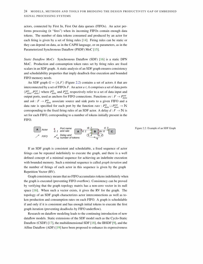
Static Dataflow MoCs Synchronous Dataflow (SDF) [16] is a static DPN
MoC. Production and consumption token rates set by firing rules are fixed
scalars in an SDF graph. A static analysis of an SDF graph ensures consistency
and schedulability properties that imply deadlock-free execution and bounded
FIFO memory needs.
An SDF graph G = (A,F) (Figure 2.2) contains a set of actors A that are
interconnected by a set of FIFOs F . An actor a∈A comprises a set of data ports
(Pindata,Pout
data) where Pindata and Pout
data respectively refer to a set of data input and
output ports, used as anchors for FIFO connections. Functions src : F → Poutdata
and snk : F → Pindata associate source and sink ports to a given FIFO and a
data rate is specified for each port by the function rate : Pindata ∪ Pout
data → N
corresponding to the fixed firing rules of an SDF actor. A delay d : F → N is
set for each FIFO, corresponding to a number of tokens initially present in the
FIFO.
A Actor
FIFO
Port nameand rate A Bd: 1 d: 1
di: 2
fi: 4 fo: 4Cdo: 6
d: 3
*4*4Delay andnumber of tokens
Figure 2.2: Example of an SDF Graph
If an SDF graph is consistent and schedulable, a fixed sequence of actor
firings can be repeated indefinitely to execute the graph, and there is a well
defined concept of a minimal sequence for achieving an indefinite execution
with bounded memory. Such a minimal sequence is called graph iteration and
the number of firings of each actor in this sequence is given by the graph
Repetition Vector (RV).
Graph consistency means that no FIFO accumulates tokens indefinitely when
the graph is executed (preventing FIFO overflow). Consistency can be proved
by verifying that the graph topology matrix has a non-zero vector in its null
space [16]. When such a vector exists, it gives the RV for the graph. The
topology of an SDF graph characterizes actor interconnections as well as to-
ken production and consumption rates on each FIFO. A graph is schedulable
if and only if it is consistent and has enough initial tokens to execute the first
graph iteration (preventing deadlocks by FIFO underflow).
Research on dataflow modeling leads to the continuing introduction of new
dataflow models. Static extensions of the SDF model such as the Cyclo-Static
Dataflow (CSDF) [17], the multidimensional SDF [18], the IBSDF [9], and the
Affine Dataflow (ADF) [19] have been proposed to enhance its expressiveness

IMPROVIN G DESI GN EFFI CI ENCY 25
and conciseness while preserving its predictability.
The Compositional Temporal Analysis (CTA) model is a non-executable
timed abstraction of the SDF MoC that can be used to analyze efficiently the
schedulability and the temporal properties of applications [20]. The IBSDF
and the CTA models both enforce the compositionality of applications. A
model is compositional if the properties (schedulability, deadlock freeness, ...)
of an application graph composed of several sub-graphs are independent from
the internal specifications of these sub-graphs [21].
Interface-Based Synchronous Dataflow MoC Interface-Based SDF (IBSDF)
[9] is a hierarchical extension of the SDF model interpreting hierarchy levels
as code closures. IBSDF fosters subgraph composition, making subgraph exe-
cutions equivalent to imperative language function calls. IBSDF has proved to
be an efficient way to model dataflow applications [11]. IBSDF interfaces are
inherited by the PiMM proposed meta-model (Section 2.3.2).
In addition to the SDF semantics, IBSDF adds interface elements to insulate
levels of hierarchy in terms of schedulability analysis. An IBSDF graph G =
(A,F , I) contains a set of interfaces I = (Iindata, Iout
data) (Figure 2.3).
A data input interface iindata ∈ Iindata in a subgraph is a vertex transmitting
to the subgraph the tokens received by its corresponding data input port. If
more tokens are consumed on a data input interface than the number of tokens
received on the corresponding data input port, the data input interface behaves
as a circular buffer, producing the same tokens several times.
A data output interface ioutdata ∈ Iout
data in a subgraph is a vertex transmitting
tokens received from the subgraph to its corresponding data output port. If a
data output interface receives too many tokens, it will behave like a circular
buffer and output only the last pushed tokens.
A Bd: 1di: 2
fi: 4 fo: 4C
do: 6d: 3
src
snk
data input interfacedata output interface
B1di1: 1
di2: 4 do2: 4
do1: 3difi
dofo
2
4
6
4
*4
Figure 2.3: Example of an IBSDF Graph
[9] details the behavior of IBSDF data input and output interfaces as well
as the IBSDF properties in terms of compositionality and schedulability check-
ing. Through PiMM, interface-based hierarchy can be applied to other dataflow
models than SDF with less restrictive firing rules.
Parameterized Dataflow MoCs Parameterized dataflow is a meta-modeling
framework introduced in [15] that is applicable to all dataflow MoCs that
present graph iterations. When this meta-model is applied, it extends the tar-
geted MoC semantics by adding dynamically reconfigurable hierarchical ac-
tors. A reconfiguration occurs when values are dynamically assigned to the

26 MODELS , METHODS AND TOOLS FO R BR IDG ING THE DESI GN PRO DUCTI VI TY GAP OF EMBEDDED
SIG NAL PROCESSI NG SY STEMS
parameters of a reconfigurable actor, causing changes in the actor computation
and in the production and consumption rates of its data ports. As presented
in [22], reconfigurations can only occur at certain points, namely quiescent
points, during the execution of a graph in order to ensure the runtime integrity
of the application.
An objective of PiMM is to further improve parameterization compared to
parameterized dataflow by introducing an explicit parameter dependency tree
and by enhancing graph compositionality. Indeed, in a PSDF graph, ports are
simple connectors between data FIFOs that do not insulate levels of hierarchy
(Section 2.3.1). Other parameterized dataflow MoCs were previously devel-
oped such as the Scenario-Aware Dataflow (SADF) [10], an analysis-oriented
model based on a probabilistic description of the dynamic firing rules of ac-
tors; or the Compaan generated KPN (CPN) [12], a parameterized extension
of the Kahn Process Network (KPN) MoC. In these models, the complexity of
the parameterization mechanism is handled by actors that can reconfigure the
firing rules of other actors (or their own) via “control channels”. This recon-
figuration mechanism differs from that of PiMM in that the latter relies on the
explicit definition of parameters and their dependencies which allows for a pre-
cise specification of what is influenced by a parameter, even in multiple levels
of hierarchy, leading to an enhanced predictability and quasi-static scheduling
potential for the model.
2.3.2 Our Contribution on Parameterized and Interfaced Dataflow
Meta-Modeling
Most of the following discussion is borrowed from our publication on PiMM
[8]. PiMM can be used similarly to the parameterized dataflow to extend the
semantics of all dataflow MoCs implementing the concept of graph iteration.
PiMM adds both interface-based hierarchy and an explicit parameter depen-
dency tree to the semantics of the extended MoC. In this section, we formally
present PiMM through its application to the SDF MoC, composing the PiSDF
model. The pictograms associated to the different elements of the PiSDF se-
mantics are presented in Figures 2.4 and 2.5.
A PiSDF graph G = (A,F , I,Π,∆) contains, in addition to the SDF actor
set A and FIFO set F , a set of hierarchical interfaces I, a set of parameters Π,
and a set of parameter dependencies ∆.
Parameterization semantics
A parameter π ∈ Π is a vertex of the graph associated to a parameter value
v∈N that is used to configure elements of the graph. For a better analyzability
of the model, a parameter can be restricted to take only values of a finite subset
of N. A configuration of a graph is the assignation of parameter values to all
parameters in Π.
An actor a ∈ A is now associated to a set of ports (Pindata, Pout
data, Pincfg, Pout
cfg )

IMPROVIN G DESI GN EFFI CI ENCY 27
where Pincfg and Pout
cfg are a set of configuration input and output ports respec-
tively. A configuration input port pincfg ∈ Pin
cfg of an actor a ∈ A is an input port
that depends on a parameter π ∈ Π and can influence the computation of a and
the production/consumption rates on the dataflow ports of a. A configuration
output port poutcfg ∈ Pout
cfg of an actor a ∈ A is an output port that can dynamically
set the value of a parameter π ∈ Π of the graph (Section 2.3.2).
A parameter dependency δ ∈ ∆ is a directed edge of the graph that links
a parameter π ∈ Π to a graph element influenced by this parameter. For-
mally a parameter dependency δ is associated to the two functions setter :
∆ → Π∪Poutcfg and getter : ∆ → Π∪Pin
cfg∪F which respectively give the source
and the target of δ . A parameter dependency set by a configuration output port
poutcfg ∈ Pout
cfg of an actor a ∈ A can only be received by a parameter vertex of the
graph that will dispatch the parameter value to other graph elements, building
a parameter dependency tree. Dynamism in PiMM relies on parameters whose
values can be used to influence one or several of the following properties: the
computation of an actor, the production/consumption rates on the ports of an
actor, the value of another parameter, and the delay of a FIFO (Section 2.3.1).
In PiMM, if an actor has all its production/consumption rates set to 0, it will
not be executed.
A parameter dependency tree T = (Π,∆) is formed by the set of parameters
Π and the set of parameter dependencies ∆. The parameter dependency tree T
is similar to a set of combinational relations where the value of each parameter
is resolved virtually instantly as a function of the parameters it depends on.
This parameter dependency tree is in contrast to the precedence graph (A,F)
where the firing of the actors is enabled by the data tokens flowing on the
FIFOs.
πSDF hierarchy semantics
The hierarchy semantics used in PiSDF inherits from the interface-based dataflow
introduced in [9] and presented in Section 2.3.1. In PiSDF, a hierarchical actor
is associated to a unique PiSDF subgraph. The set of interfaces I of a sub-
graph is extended as follows: I = (Iindata, Iout
data, Iincfg, Iout
cfg ) where Iincfg is a set of
configuration input interfaces and Ioutcfg a set of configuration output interfaces.
Configuration input and output interfaces of a hierarchical actor are respec-
tively seen as a configuration input port pincfg ∈ Pin
cfg and a configuration output
port poutcfg ∈ Pout
cfg from the upper level of hierarchy (Section 2.3.2).
From the subgraph perspective, a configuration input interface is seen as a
locally static parameter whose value is left undefined.
A configuration output interface enables the transmission of a parameter
value from the subgraph of a hierarchical actor to upper levels of hierarchy.
In the subgraph, this parameter value is provided by a FIFO linked to a data
output port poutdata of an actor that produces data tokens with values v ∈ N. In
cases where several values are produced during an iteration of the subgraph, the
configuration output interface behaves like a data output interface of size 1 and

28 MODELS , METHODS AND TOOLS FO R BR IDG ING THE DESI GN PRO DUCTI VI TY GAP OF EMBEDDED
SIG NAL PROCESSI NG SY STEMS
only the last value written will be produced on the corresponding configuration
output port of the enclosing hierarchical actor (Section 2.3.1).
Figure 2.4 presents an example of a static PiSDF description. Compared
to Figure 2.3, it introduces parameters and parameter dependencies that com-
pose a PiMM parameter dependency tree. The modeled example illustrates the
modeling of a test bench for an image processing algorithm. In the example,
one token corresponds to a single pixel in an image. Images are read, pixel
by pixel, by actor A and stored, pixel by pixel, by actor C. A whole image is
processed by one firing of actor B. A feedback edge with a delay stores the
previous image for comparison with the current one. Actor B is refined by an
actor B1 processing one Nth of the image. In Figure 2.4, the size of the image
picsize and the parameter N are locally static.
N
di: picsize/N do: picsize/N
A Bd: 1
picsize
C
picsize
d: 1
B1
difi
dofo
picsize
size locally staticparameter
parameterdependency
configurationinput port
*picsize
picsize picsizefi: picsize/N fo: picsize/N
configurationinput interface
Figure 2.4: Example of a PiSDF Graph with
Static Parameters
πSDF Reconfiguration As introduced in [22], the frequency with which the
value of a parameter is changed influences the predictability of the applica-
tion. A constant value will result in a high predictability while a value which
changes at each iteration of a graph will cause many reconfigurations, thus
lowering the predictability.
There are two types of parameters π ∈Π in PiSDF: configurable parameters
and locally static parameters. Both restrict how often the value of the parameter
can change. Regardless of the type, a parameter must have a constant value
during an iteration of the graph to which it belongs.
Configurable parameters
A configurable parameter πcfg ∈ Π is a parameter whose value is dynamically
set once at the beginning of each iteration of the graph to which it belongs.
Configurable parameters can influence all elements of their subgraph except
the production/consumption rates on the data interfaces Iindata and Iout
data. As ex-
plained in [15], this restriction is essential to ensure that, as in IBSDF, a parent
graph has a consistent view of its actors throughout an iteration, even if the
topology may change between iterations.
The value of a configurable parameter can either be set through a param-
eter dependency coming from an other configurable parameter or through a

IMPROVIN G DESI GN EFFI CI ENCY 29
parameter dependency coming from a configuration output port poutcfg of a con-
figuration actor (Section 2.3.2). In Figure 2.5, N is a configurable parameter.
Locally static parameters
A locally static parameter πstat ∈ Π of a graph has a value that is set before the
beginning of the graph execution and which remains constant over one or sev-
eral iterations of this graph. In addition to the properties listed in Section 2.3.2,
a locally static parameter belonging to a subgraph can also be used to influence
the production and consumption rates on the Iindata and Iout
data interfaces of its hi-
erarchical actor.
The value of a locally static parameter can be statically set at compile time,
or it can be dynamically set by configurable parameters of upper levels of hi-
erarchy via parameter dependencies. For example, a subgraph sees a config-
uration input interface as a locally static parameter but this interface can take
different values at runtime if its corresponding configuration input port is con-
nected to a configurable parameter. In Figure 2.5, picsize is a locally static
parameter both in main graph and in subgraph B.
A partial configuration state of a graph is reached when the parameter val-
ues of all its locally static parameters are set. Hierarchy traversal of a hierar-
chical actor is possible only when the corresponding subgraph has reached a
partial configuration state.
A complete configuration state of a graph is reached when the values of
all its parameters (locally static and configurable) are set. If a graph does not
contain any configurable parameter, its partial and complete configurations are
equivalent. Only when a graph is completely configured is it possible to check
its consistency, compute a schedule, and execute it.
Configuration Actors
A firing of an actor a with a configuration output port poutcfg produces a pa-
rameter value that can be used via a parameter dependency δ to dynamically
set a configurable parameter π (Section 2.3.2), provoking a reconfiguration
of the graph elements depending on π . In PiMM, such an actor is called a
configuration actor. The execution of a configuration actor is the cause of a
reconfiguration and must consequently happen only at quiescent points during
the graph execution, as explained in [22]. To ensure the correct behavior of
PiSDF graphs, a configuration actor acfg ∈ A of a subgraph G is subject to the
following restrictions:
R1. acfg must be fired exactly once per iteration of G before the firing of any
non-configuration actor. Indeed, G reaches a complete configuration only
when all its configuration actors have fired.
R2. acfg must consume data tokens only from hierarchical interfaces of G and
must consume all available tokens during its unique firing.

30 MODELS , METHODS AND TOOLS FO R BR IDG ING THE DESI GN PRO DUCTI VI TY GAP OF EMBEDDED
SIG NAL PROCESSI NG SY STEMS
R3. The production/consumption rates of a acfg can only depend on locally
static parameters of G.
R4. Data tokens produced by acfg are seen as a data input interface by other
actors of G. (i.e. they are made available using a ring-buffer and can be
consumed more than once).
These restrictions naturally enforce the local synchrony conditions of parame-
terized dataflow defined in [15] and reminded in Section 2.3.2.
The firing of all configuration actors of a graph is needed to obtain a com-
plete configuration of this graph. Consequently, configuration actors will al-
ways be executed before other (non-configuration) actors of the graph to which
they belong. Configuration actors are the only actors whose firing is not data-
driven but driven by hierarchy traversal.
The sets of configuration and non-configuration actors of a graph are respec-
tively equivalent to the subinit φs and the body φb subgraphs of parameterized
dataflow [15]. Nevertheless, configuration actors provide more flexibility than
subinit graphs as they can produce data tokens that will be consumed by non-
configuration actors of their graph. The init subgraph φi has no equivalent
in PiMM as its responsibility, namely the configuration of the production/-
consumption rates on the actor interfaces, is performed by configuration input
interfaces and parameter dependencies.
Figure 2.5 presents an example of a PiSDF description with reconfiguration.
It is a modified version of the example in Figure 2.4 presented in Section 2.3.2.
In Figure 2.5, the parameter N is a configurable parameter of subgraph B, while
the parameter picsize is a locally static parameter. The number of firings of ac-
tor B1 for each firing of actor B is dynamically configured by the configuration
actor setN. In this example, the dynamic reconfiguration dynamically adapts
the number N of firings of B1 to the number of cores available to perform the
computation of B. Indeed, since B1 has no self-loop FIFO, the N firings of B1
can be executed concurrently.
configurationoutput port
Aconfigurationactor
di: picsize/N do: picsize/N
A Bd: 1
picsize
C
picsize
d: 1
B1
difi
dofo
picsize
*picsize
picsize picsizefi: picsize/N fo: picsize/N
setNdi: picsize N
configurableparameterN
Figure 2.5: Example of a PiSDF Graph with
Reconfiguration
Model Analysis and Behavior The PiSDF MoC presented in Section 2.3.2
is dedicated to the specification of applications with both dynamic and static

IMPROVIN G DESI GN EFFI CI ENCY 31
parameterizations. This dual degree of dynamism implies a two-step analysis
of the behavior of applications described in PiSDF: a compile time analysis
and a runtime analysis. In each step a set of properties of the application can be
checked, such as the consistency, the deadlock freeness, and the boundedness.
Other operations can be performed during one or both steps of the analysis such
as the computation of a schedule or the application of graph transformation to
enhance the performance of the application.
Compile Time Schedulability Analysis PiSDF inherits its schedulability prop-
erties both from the interface-based dataflow modeling and the parameterized
dataflow modeling.
In interface-based dataflow modeling, as proved in [9], a (sub)graph is
schedulable if its precedence SDF graph (A,F) (excluding interfaces) is con-
sistent and deadlock-free. When a PiSDF graph reaches a complete configura-
tion, it becomes equivalent to an IBSDF graph. Given a complete configura-
tion, the schedulability of a PiSDF graph can thus be checked using the same
conditions as in interface-based dataflow.
In parameterized dataflow, the schedulability of a graph can be guaranteed
at compile time for certain applications by checking their local synchrony [15].
A PSDF (sub)graph is locally synchronous if it is schedulable for all reachable
configurations and if all its hierarchical children are locally synchronous. As
presented in [15], a PSDF hierarchical actor composed of three subgraphs φi,
φs and φb must satisfy the 5 following conditions in order to be locally syn-
chronous:
1. φi, φs and φb must be locally synchronous, i.e. they must be schedulable for
all reachable configurations.
2. Each invocation of φi must give a unique value to parameter set by this
subgraph.
3. Each invocation of φs must give a unique value to parameter set by this
subgraph.
4. Consumption rates of φs on interfaces of the hierarchical actor cannot de-
pend on parameters set by φs.
5. Production/consumption rates of φb on interfaces of the hierarchical actor
cannot depend on parameters set by φs.
The last four of these conditions are naturally enforced by the PiSDF seman-
tics presented in Section 2.3.2. However, the schedulability condition number
1., which states that all subgraphs must be schedulable for all reachable con-
figurations, cannot always be checked at compile time. Indeed, since values of
the parameters are freely chosen by the application developer, non-schedulable
graphs can be described. It is the responsibility of the developer to make sure

32 MODELS , METHODS AND TOOLS FO R BR IDG ING THE DESI GN PRO DUCTI VI TY GAP OF EMBEDDED
SIG NAL PROCESSI NG SY STEMS
that an application will always satisfy the schedulability condition; this respon-
sibility is similar to that of writing non-infinite loops in imperative languages.
PiSDF inherits from PSDF the possibility to derive quasi-static schedules at
compile time for some applications. A quasi-static schedule is a schedule that
statically defines part of the scheduling decisions but also contains parameter-
ized parts that will be resolved at runtime.
2.3.3 Comparison or PiMM with other MoCs
Table 2.1 presents a comparison of dataflow MoCs based on a set of common
MoC features. The compared MoCs include the static SDF [16], ADF [19],
and IBSDF [9]. Also compared are the dynamic PSDF [15], SADF [10],
DPN [13], and PiSDF.
In Table 2.1, a black dot indicates that the feature is implemented by a
MoC, an absence of dot means that the feature is not implemented, and an
empty dot indicates that the feature may be available for some applications
described with this MoC. It is important to note that the full semantics of the
compared MoCs is considered here. Indeed, some features can be obtained by
using only a restricted semantics of other MoCs. For example, all MoCs can
be restricted to describe a SDF, thus benefiting from the static schedulability
and the decidability but losing all reconfigurability.
Feature SDFADF
IBSDF
PSDFPiS
DF
SADF
DPN
Hierarchy • • •
Compositional • •
Reconfigurable • • • •
Configuration dependency • •
Statically schedulable • • •
Decidability • • • ◦ ◦ •
Variable rates • • • • •
Non-determinism • •
Table 2.1: Features comparison of different
dataflow MoCs
The features compared in Table 2.1 are the following: Hierarchy: compos-
ability can be achieved by associating a subgraph to an actor. Compositional:
graph properties are independent from the internal specifications of the sub-
graphs that compose it [21]. Reconfigurable: actors firing rules can be recon-
figured dynamically. Configuration dependency: the MoC semantics includes
an element dedicated to the transmission of configuration parameters. Stati-
cally schedulable: a fully static schedule can be derived at compile time [16].
Decidability: the schedulability is provable at compile time. Variable rates:
production/consumption rates are not a fixed scalar. Non-determinism: output
of an algorithm does not solely depends on inputs, but also on external factors
(e.g. time, randomness).
In the next section on system adaptivity, we put the focus on using the

IMPROVIN G DESI GN EFFI CI ENCY 33
PiSDF model to efficiently use the resources of a system even in the case of
highly variable application, and this without requiring additional design effort.
2.4 System Adaptivity
A system is qualified as adaptive when it can use variations on application
loads to save resources and optimize Non-Functional Properties. Adaptivity
also refers to the capacity to receive, at runtime, a new application, adapt to
it and resume execution. We have started in the PhD thesis of El Mehdi Ab-
dali a study of adaptive systems for hardware-defined applications using the
Dynamic and Partial Reconfiguration (DPR) capabilities of modern FPGAs.
In the former PhD thesis of Julien Heulot, we have targeted software-defined
systems over heterogeneous multi-core architectures and a dynamic schedul-
ing method has been developed for the PiSDF MoC. The following discussion
has been published in the Proceedings of the GlobalSIP 2014 conference5. 5 Julien Heulot, Maxime Pelcat, Jean-
François Nezan, Yaset Oliva, Slaheddine
Aridhi, and Shuvra S Bhattacharyya. Just-
in-time scheduling techniques for multicore
signal processing systems. In Proceedings of
the GlobalSIP conference. IEEE, 2014
The proposed scheduling method, named JIT-MS, aims to efficiently sched-
ule PiSDF graphs on multicore architectures. This method exploits features of
PiSDF to find locally static regions that exhibit predictable communications.
As evoked in the introduction of this report, embedded processors contain
an increasingly number of cores [24, 25, 26]. This trend is mainly due to limi-
tations in the processing power of individual PEs as a result of power consump-
tion considerations. Concurrently, signal processing applications are becoming
increasingly dynamic in terms of hardware resource requirements. For exam-
ple, the Scalable High Efficiency Video Coding (SHVC) standard provides a
mechanism to temporarily reduce the resolution of a transmitted video in order
to match the instantaneous bandwidth of a network [27].
One of the main challenges of the design of multicore signal processing
systems is to distribute computational tasks efficiently onto the available PEs
while taking into account dynamic application and architecture changes. The
process of assigning, ordering and timing actors on PEs in this context is re-
ferred to as multicore scheduling. Inefficient use of the PEs affects latency and
energy consumption, making multicore scheduling an important challenge [28].
JIT-MS addresses this challenge. JIT-MS is a flexible scheduling method that
determines scheduling decisions at run-time to optimize the mapping of an ap-
plication onto multicore processing resources. In relation to the scheduling
taxonomy defined by Lee and Ha [29], JIT-MS is a fully dynamic schedul-
ing strategy. In the context of the taxonomy used in Singh’s survey [30], our
method can be classified as “On-the-fly” mapping, targeting heterogeneous
platforms with a centralized resource management strategy.
JIT-MS exploits the fact that between two quiescent points[22], the applica-
tion can be considered static. Decisions are taken Just-In-Time, immediately
after the quiescent points are reached, unveiling new application parallelism.
Various competing frameworks based on OpenMP [31] and OpenCL [32]
language extensions are currently proposed to address the multicore schedul-

34 MODELS , METHODS AND TOOLS FO R BR IDG ING THE DESI GN PRO DUCTI VI TY GAP OF EMBEDDED
SIG NAL PROCESSI NG SY STEMS
ing challenge. However, these extensions are based on imperative languages
(e.g., C, C++, Fortran) that do not provide mechanisms to model specific signal
flow graph topologies. In the experimental results on this section we demon-
strate that JIT-MS is capable of challenging, on an 8-core DSP processor, an
OpenMP implementation provided by Texas Instruments. Latency improve-
ments of up to 26% are observed, obtained because advanced information is
known by the runtime manager on the application. The next sections detail
JIT-MS.
2.4.1 Context
Runtime Architecture JIT-MS is applicable to heterogeneous platforms. On
such platforms, a locally optimal decision to fire an actor (e.g., based on the
availability of its input data) can be inefficient when considering the system
globally. In order to take effective decisions globally, a Master/Slave execution
scheme is chosen for the system.
Scheduling
ElementProcessing
Element
Processing
Element
Parameters
Jobs
Jobs
Parameters
Data
Tokens
Figure 2.6: JIT-MS Runtime execution
scheme.
The JIT-MS method relies on multiple software or hardware Processing
Elements (PEs) that are slave components responsible for processing actors
(Figure 2.6). PEs can be of multiple types, such as General Purpose Processors
(GPPs), DSPs, or hardware accelerators. The master processor of the JIT-MS
system is called Scheduling Element (SE). This is the only component that
has access to the general algorithm topology. Jobs are used to communicate
between the SE and PEs. Each PE has a job queue from which it pops jobs
out prior to their execution. Parameters influence dataflow graph topology or
execution timing of actors. When a parameter value is set by a configuration
actor, its value is sent to the SE via a parameter queue. Finally, Data FIFOs
are used by the PEs to exchange data tokens. A data FIFO can be implemented
either over a shared memory or over network-on-chip communication.
Benchmark We illustrate the JIT-MS scheduling algorithm in this report by
the scheduling of a benchmark application. This benchmark is an extension of
the MP-sched benchmark [33]. The MP-sched benchmark can be viewed as
a two-dimensional grid involving N channels, where each branch consists of
M cascaded Finite Impulse Response (FIR) filters of NbS samples. We extend

IMPROVIN G DESI GN EFFI CI ENCY 35
the MP-sched benchmark by allowing the M parameter to vary across different
branches, as illustrated in Figure 2.7. We refer to this extended version of
the MP-sched benchmark as heterogeneous-chain-length MP-sched (HCLM-
sched).
Figure 2.7: Description of the HCLM-Shed
benchmark used to test JIT-MS scheduling.
A PiSDF representation of the HCLM-sched benchmark is shown in Fig-
ure 2.8. To represent the channels in the HCLM-sched benchmark, a hierar-
chical actor called FIR_Chan is introduced. The top level graph is designed
to repeat N times this actor. In the subgraph describing the behavior of the
FIR_Chan actor, M pipelined FIR filter repetitions in the branches are handled
by a feedback loop and specific control actors (Init, Switch and Broadcast).
N
FIR_Chan
in out
MSrcsrcN
SnkN
snk
configN
M
NbS N*NbSN*NbS Nbs
In
Out
MM
1
Nmax
MFilter
M
N
MNNmax
NbS
NbS
NbS
NbS
NbS
NbS
NbS
NbSNbS NbSNbS
Figure 2.8: A PiSDF model of the HCLM-
sched benchmark.
Notations To describe JIT-MS, the following notation is used. CA represents
the set of configuration actors of the given PiSDF graphand CA represents all
actors in the given PiSDF graph that are not configuration actors.
2.4.2 Just-In-Time Multicore Scheduling (JIT-MS)
Multicore Scheduling of Static Subgraphs JIT-MS involves decomposing the
scheduling of a given PiSDF graph into the scheduling of a sequence X1,X2, . . .
of SDF graphs. Different executions (with different sets of input data) can
result in different sequences of SDF graphs for the same PiSDF graph. For
a given execution, we refer to each Xi as a step of the JIT-MS scheduling
process. At each step, resolved parameters trigger the transformation of the

36 MODELS , METHODS AND TOOLS FO R BR IDG ING THE DESI GN PRO DUCTI VI TY GAP OF EMBEDDED
SIG NAL PROCESSI NG SY STEMS
PiSDF graph into an SDF graph, which can be scheduled by any of the numer-
ous existing SDF scheduling heuristics that are relevant for multicore architec-
tures [34]. For example, [35] presents a set of techniques that can be applied
upon transforming the resulting SDF graph into an single rate SDF (srSDF)
graph. An srSDF graph is an SDF graph in which the production rate on each
edge is equal to the consumption rate on that edge. A consistent SDF graph
can be transformed into an equivalent srSDF graph for instance by applying
techniques that were introduced by Lee and Messerschmitt [36].
The Just-In-Time Multicore Scheduling (JIT-MS) method is based on a
static multicore scheduling method which is composed of the following se-
quence of phases:
1. Computing the Repetition Vector (RV) of the current graph (the graph that
is presently being scheduled). The RV is a positive-integer vector and rep-
resents the number of firings of each actor in a minimal periodic scheduling
iteration for the graph. We note however, that certain technical details of
PiSDF require adaptations to the conventional repetitions vector computa-
tion process from [16].
2. Converting the SDF graph into an equivalent srSDF graph, where each ac-
tor is instantiated a number of times equal to its corresponding RV compo-
nent.
3. Scheduling actors and communications from a derived acyclic srSDF graph
onto the targeted heterogeneous platform. Any scheduling heuristic that is
applicable to acyclic srSDFs graphs can be chosen here — e.g., the applied
schedule can be a list scheduler, fast scheduler, flow-shop or genetic sched-
uler [30, 37, 35]. Upon completing the described scheduling process, the
resulting schedule S is executed.
A complete JIT-MS schedule of a PiSDF hierarchical graph consists of sev-
eral of these phases, repeated as many times as needed.
In a PiSDF graph, some data FIFOs behave as Round Buffers (RBs) — i.e.,
such FIFOs produce multiple copies of individual tokens as necessary to sat-
isfy consumption demand. In particular, FIFOs at the interface of a hierarchical
actor have RBs behavior to help ensure composability in hierarchical specifi-
cations. FIFOs connecting configuration actors to other actors also behave as
RBs to ensure that configuration actors fire only once per subgraph. Applica-
tion designers using the PiSDF model of computation need to take such RB
behavior into account during the development process.
Configuration Actors and such RBs are excluded from the RV computation
as they are forced to fire only once.
Multicore Scheduling of Full Graphs The JIT-MS method is based on the
PiSDF runtime operational semantic. As shown in [8], the JIT-MS scheduler
has to proceed in multiple steps, each one unveiling a new portion of srSDF

IMPROVIN G DESI GN EFFI CI ENCY 37
graph for scheduling. In one step, configuration actors have to be fired first,
they produce parameters needed to resolve the rest of the subgraph. When all
parameters are solved at one hierarchy level, scheduling of other actors of this
hierarchy level is made possible. The complete srSDF graph is only known
when all configuration actors have been executed.
Once an srSDF graph has been generated, it can be analyzed to exploit
the parallelism of the application (Section 2.4.2). The JIT-MS runtime sched-
ules the actors and communications and fires their execution on the platform.
Newly instantiated hierarchical actors are added to a global srSDF graph, called
execution graph, and the same process can be used until the whole graph has
been processed.
To keep track of actor’s execution, each actor of the execution graph is
tagged with a flag representing its execution state. An actor can be Run (R),
Not Executable (N) or Executable (E). An actor is Executable only when all its
parameters are resolved and when all its predecessors are Executable or Run.
CfgM
RBI O
10 10
Srcsrc
MFilMM
FIR_CM
I OSnksnk
FIR_CM
I O
Join
I1 O
I0
2
8000
1
4000
1
4000
Fork
I
O0
O1
Fork
I
O0
O1
4000
4000 8000
CfgM
RBI O
10 10
Srcsrc
MFilMM
Snksnk
Join
I1 O
I0
2
8000
1
4000
1
4000
Fork
I
O0
O1
Fork
I
O0
O1
4000
4000 8000
RBI O
RBI O
RBI O
RBI O
RBI O
RBI O
SMM
SMM
1
1
CfgM
RBI O
10 10
Srcsrc
MFilMM
Snksnk
Join
I1 O
I0
2
8000
1
4000
1
4000
Fork
I
O0
O1
Fork
I
O0
O1
4000
4000 8000
RBI O
RBI O
RBI O
RBI O
RBI O
RBI O
SMM
SMM
1
1
Initsel
Sw
O
seli0
i1
FIROI
Br
I
O0
O1
Fork
I
O1
O0
Fork
I
O0
O1
Join
I0 O
I1
1
4000
4000 4000
4000
Initsel
Sw
O
seli0
i1
FIROI
Br
I
O0
O1
2
4000
4000 4000
8000
1
Sw
O
seli1
i0
FIROI
Br
I
O0
O14000 4000
4000
4000
4000
4000
4000
1
8000
4000
CfgM
RBI O
10
a) Loop I.a b) Loop I.b c) Loop II.a
d) Loop II.b
Figure 2.9: single rate SDFs (srSDFs) graphs
generated from the HCLM-sched benchmark
of Figure 2.8. Blue actors are not executable,
green ones are executable and black ones are
already run. Red dashed actors are hierarchi-
cal.
Applying JIT-MS to the Benchmark The execution graph shape at each step
of the HCLM-sched benchmark can be seen in Figure 2.9.
Figure 2.9.a corresponds to the execution graph state at the end of the first
phase of the first iteration of the while loop (loop I.a). At this point, N is set
to 2. Then Figure 2.9.b corresponds to execution graph state after the third
phase of the first iteration (loop I.b). The hierarchical FIR_Chan actors are
instanciated. Then, Figures 2.9.c and 2.9.d correspond to the execution, first of
the internal configuration actors of FIR_Chan (SM), then of their actors with
parameter M = {1,2}.

38 MODELS , METHODS AND TOOLS FO R BR IDG ING THE DESI GN PRO DUCTI VI TY GAP OF EMBEDDED
SIG NAL PROCESSI NG SY STEMS
2.4.3 Experimental Results
The main goal of JIT-MS is to parallelize dynamic applications. The following
experimental results focus on the comparison between the JIT-MS approach
and an OpenMP runtime system with similar objectives. Results are acquired
by studying the latency of single and multiple iterations of the HCLM-sched
benchmark on a Texas Instruments TMS320C6678 multicore DSP processor
[24].
OpenMP is a framework designed for shared memory multiprocessing. It
provides mechanisms for launching parallel teams of threads to execute an al-
gorithm on a multicore architecture. OpenMP applications are designed with
a succession of sequential code sections, executed by a master thread, and par-
allel code sections, distributed in a team of threads dispatched onto multiple
cores [31]. The c6678 processor is composed of 8 c66x DSP cores intercon-
nected by a NoC called TeraNet with access to an internal shared memory.
To perform synchronization between cores, hardware queues provided by the
Texas Instruments Multicore Navigator[38] have been used in this study.
Results on execution time are displayed in Figure 2.10.a.
1e+06
1.5e+06
2e+06
2.5e+06
3e+06
3.5e+06
7 8 9 10 11 12 13 14 15 16 17
Late
ncy (
cycle
s)
N
JIT-MSOpenMP
Figure 2.10: JIT-MS Latency versus values
of N for the HCLM-sched benchmark
Experimental results of Figure 2.10 show that the OpenMP implementa-
tion latency curve displays a step shape when increasing N. With the JIT-MS
implementation, the graph transformation and scheduling phases introduce an
overhead but the execution efficiency over varying parameters is smoother. The
overhead can be observed on the figure when N equals to 7 or 8 as the result-
ing scheduling is the same as OpenMP. The transformation to srSDF extracts
more parallelism than OpenMP from the subdivision of channels into multiple
FIRs. These choices make JIT-MS suitable for unbalanced applications. In the
HCLM-sched benchmark with 9 channels, the overall latency is reduced of up
to 26%. Figures 2.11 and 2.12 illustrate this effect by displaying the real Gantt
chart of execution, based on measurements from the internal processor timer.
Spider scheduling is shown to introduce an initial latency due to graph manage-
ment (the red block on the left of Figure 2.12) but then efficiently interleaves
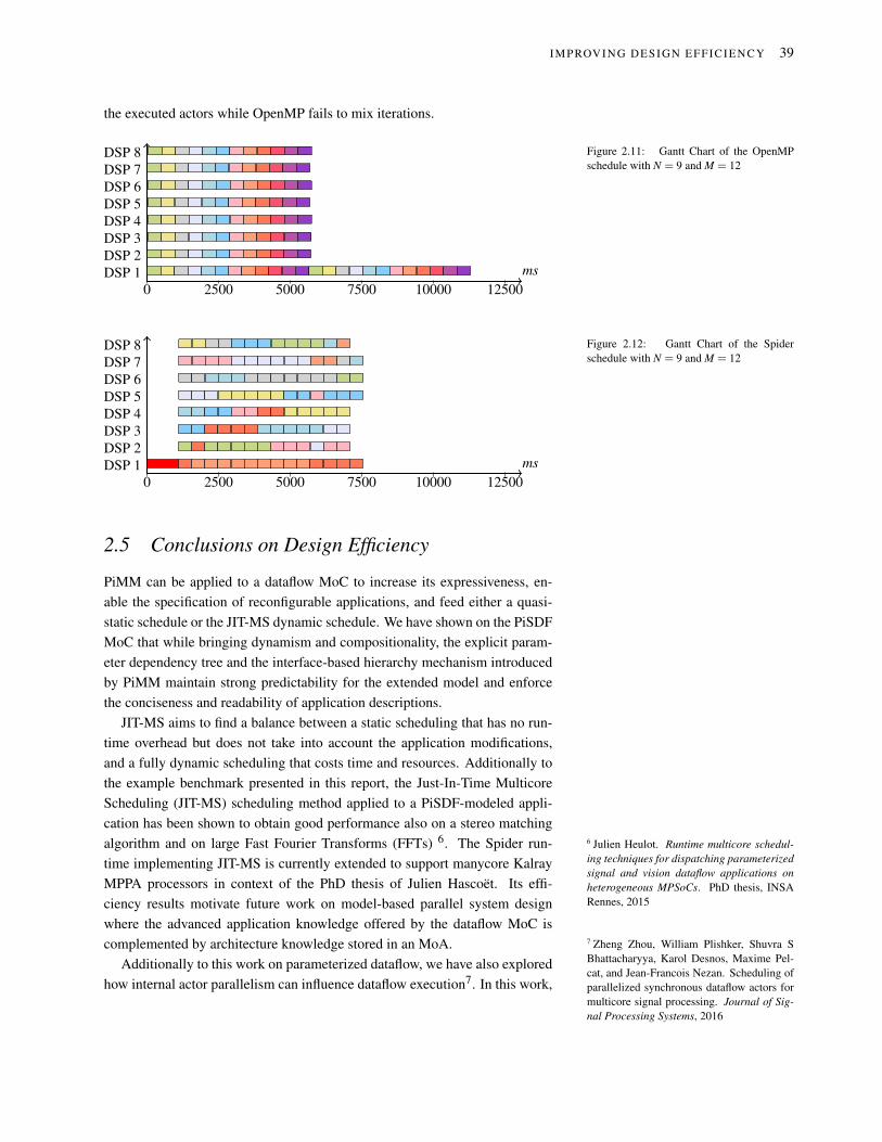
IMPROVIN G DESI GN EFFI CI ENCY 39
the executed actors while OpenMP fails to mix iterations.
0 2500 5000 7500 10000 12500
msDSP 1
DSP 2
DSP 3
DSP 4
DSP 5
DSP 6
DSP 7
DSP 8 Figure 2.11: Gantt Chart of the OpenMP
schedule with N = 9 and M = 12
0 2500 5000 7500 10000 12500
msDSP 1
DSP 2
DSP 3
DSP 4
DSP 5
DSP 6
DSP 7
DSP 8 Figure 2.12: Gantt Chart of the Spider
schedule with N = 9 and M = 12
2.5 Conclusions on Design Efficiency
PiMM can be applied to a dataflow MoC to increase its expressiveness, en-
able the specification of reconfigurable applications, and feed either a quasi-
static schedule or the JIT-MS dynamic schedule. We have shown on the PiSDF
MoC that while bringing dynamism and compositionality, the explicit param-
eter dependency tree and the interface-based hierarchy mechanism introduced
by PiMM maintain strong predictability for the extended model and enforce
the conciseness and readability of application descriptions.
JIT-MS aims to find a balance between a static scheduling that has no run-
time overhead but does not take into account the application modifications,
and a fully dynamic scheduling that costs time and resources. Additionally to
the example benchmark presented in this report, the Just-In-Time Multicore
Scheduling (JIT-MS) scheduling method applied to a PiSDF-modeled appli-
cation has been shown to obtain good performance also on a stereo matching
algorithm and on large Fast Fourier Transforms (FFTs) 6. The Spider run- 6 Julien Heulot. Runtime multicore schedul-
ing techniques for dispatching parameterized
signal and vision dataflow applications on
heterogeneous MPSoCs. PhD thesis, INSA
Rennes, 2015
time implementing JIT-MS is currently extended to support manycore Kalray
MPPA processors in context of the PhD thesis of Julien Hascoët. Its effi-
ciency results motivate future work on model-based parallel system design
where the advanced application knowledge offered by the dataflow MoC is
complemented by architecture knowledge stored in an MoA.
Additionally to this work on parameterized dataflow, we have also explored
how internal actor parallelism can influence dataflow execution7. In this work,
7 Zheng Zhou, William Plishker, Shuvra S
Bhattacharyya, Karol Desnos, Maxime Pel-
cat, and Jean-Francois Nezan. Scheduling of
parallelized synchronous dataflow actors for
multicore signal processing. Journal of Sig-
nal Processing Systems, 2016

40 MODELS , METHODS AND TOOLS FO R BR IDG ING THE DESI GN PRO DUCTI VI TY GAP OF EMBEDDED
SIG NAL PROCESSI NG SY STEMS
a type of parallel task scheduling problem called Parallel Actor Scheduling
(PAS) has been defined. It combines intra- and inter-actor parallelism for plat-
forms in which individual actors can be parallelized across multiple cores. We
demonstrated that the PAS-targeted scheduling framework provides a useful
range of trade-offs between synthesis time requirements and the quality of the
derived solutions.
The UML Modeling And Analysis Of Real-Time Embedded Systems (MARTE)
standard defines semantics close to the PiSDF model to represent applications.
We have, in collaboration with Ecole Nationale d’Ingénieurs de Sfax (ENIS),
demonstrated the compatibility of the UML MARTE model with PiSDF and
the possibility to generate PiSDF from a UML MARTE compliant model and
derive Design Space Exploration (DSE) results from this generated model 8. 8 Manel Ammar, Mouna Baklouti, Maxime
Pelcat, Karol Desnos, and Mohamed Abid.
Marte to πsdf transformation for data-
intensive applications analysis. In Proceed-
ings of the DASIP Conference. IEEE, 2014
All our studies on PiSDF are implemented in the PREESM tool9 available on
9 M. Pelcat, K. Desnos, J. Heulot, C. Guy,
J.-F. Nezan, and S. Aridhi. PREESM: A
dataflow-based rapid prototyping framework
for simplifying multicore dsp programming.
In Proceedings of the EDERC Conference,
Sept 2014
Github:
http://preesm.sourceforge.net.
In the next chapter, PiSDF is also employed but this time for improving the
Non-Functional Properties (NFPs) of the built system and increase its imple-
mentation quality.

3
Improving Implementation Quality
Implementation quality
Non-Functional Property (NFP
) cos
ts
Figure 3.1: Improving implementation qual-
ity on the DP chart.
3.1 Chapter Abstract
After the previous chapter looking into the reduction of design efforts, this
chapter puts the focus on the Non-Functional Properties (NFPs) of DSP sys-
tems we aim to optimize. The latency (time between input and output) and
throughput (acceptable input rate) real-time NFPs are historically the main
optimized properties by compilers and tools and solutions exist in the litera-
ture to optimize and guarantee them. We have thus focused on the NFPs that
are often the other main concerns of designers: the energy consumption and
the memory footprint.
Memory is often very limited in embedded systems compared to the mem-
ory required by modern DSP algorithms. As a consequence, complex hardware
and software features are used to fit the application into the platforms. Based
on the PiSDF MoC, we have studied pre-scheduling and post-scheduling au-
tomated memory allocations methods, and computed memory bounds for de-
ciding early whether a platform can execute or not a given application. Pre-
scheduling and post-scheduling memory allocations have been compared and
memory bounds computed for deciding early whether a platform can execute
or not a given application. Finally, aggressive memory optimizations have
been obtained using additional information on the internal actor behavior re-
garding memory access types and order. A Domain specific language (DSL)
has been created to capture this behavior and feed the memory optimization
process. The resulting compilation process has been demonstrated to gain
substantial memory when compared to state-of-the-art methods.
In terms of energy consumption, we have observed that modern multi-
core platforms with Dynamic Voltage and Frequency Scaling (DVFS) and
Dynamic Power Management (DPM) capabilities present a non-trivial en-
ergy consumption behavior. Depending on the parallelism of the application,
the latency constraints and the static and dynamic power consumption of the
platform, different strategies should be adopted and neither the As-Slow-As-
Possible (ASAP) nor the As-Fast-As-Possible (AFAP) actor execution strate-

42 MODELS , METHODS AND TOOLS FO R BR IDG ING THE DESI GN PRO DUCTI VI TY GAP OF EMBEDDED
SIG NAL PROCESSI NG SY STEMS
gies obtains the optimal energy consumption. These first results encourage us
to explore further the use of dataflow information for driving complex MPSoC
platforms.
3.2 Using Dataflow Application Representations to
Improve System Non-Functional Properties
Real-time processing is the main NFP a DSP system must respect. Ensuring
real-time (in terms of either latency or throughput) is compulsory and the pre-
dictability of PiSDF is particularly useful for obtaining time guarantees. The
State of the Art of real-time multicore scheduling of dataflow modeled applica-
tions is rich. As a consequence, we have mostly used methods from literature
for mapping and scheduling actors to multiple cores and worked on extending
these methods to balancing the loads over the available cores1. 1 Maxime Pelcat, Slaheddine Aridhi,
Jonathan Piat, and Jean-François Nezan.
Physical Layer Multi-Core Prototyping: A
Dataflow-Based Approach for LTE eNodeB.
Springer, 2012
The two NFPs we extensively studied in the past years from PiSDF de-
scribed applications are memory consumption and energy consumption.
In terms of memory consumption, dataflow MoCs, including PiSDF, tend
to favor parallelism to the detriment of memory consumption. Within the PhD
thesis of Karol Desnos, this drawback has been eliminated and state-of-the-art
memory allocation techniques defined.
In terms of energy consumption, battery powered systems represent a large
share of embedded systems. Energy consumption is thus certainly the second
most important NFP after real-time. The reduction of the computational en-
ergy consumption has been studied during the PhD thesis of Erwan Nogues
and experimented on use case implementations of the MPEG High Efficiency
Video Coding (HEVC) standard. New strategies of energy reduction have been
designed, in particular from PiSDF application descriptions.
The next sections give some insights on these memory and energy studies.
3.3 Dataflow Memory Optimizations
Having a predictable model of an application such as PiSDF, the causality of
the actors in the application is precisely known and this information can be
employed to reuse memory between different parts of an application.
Within the PhD thesis of Karol Desnos, we have covered several aspects of
memory allocation on a multicore platform from a static dataflow description
of an application 2. 2 Karol Desnos. Memory Study and Dataflow
Representations for Rapid Prototyping of
Signal Processing Applications on MPSoCs.
PhD thesis, INSA Rennes, 20143.3.1 Computing Upper and Lower Memory Bounds
We have computed upper and lower bounds for the amount of memory to be
allocated to implement an application described with SDF3. The First In, First 3 Karol Desnos, Maxime Pelcat,
Jean François Nezan, and Slaheddine
Aridhi. Memory Bounds for the Distributed
Execution of a Hierarchical Synchronous
Data-Flow Graph. In Proceedings of the
IC-SAMOS Conference, 2012
Out data queues (FIFOs) used to exchange data between SDF actors can either
be allocated without reusing memory between them or different methods can

I MPROVIN G I MPLEMENTATION QUA LITY 43
be used to allocate them in overlapping memory locations. If no memory reuse
is employed, the size of the memory footprint can be very high, due to the
potentially large number of FIFOs employed to decouple actors’ executions.
A PiSDF application representation with static parameters being convertible to
an SDF graph, this study is applicable to static PiSDF applications.
To compute the bounds, a graph representing FIFO exclusions is built from
the original SDF graph. This graph is called Memory Exclusion Graph (MEG)
and can be studied to characterize the application memory consumption. Fig-
ures 3.2, 3.3 and 3.4 display on an example the bound computation procedure.
As shown in Figure 3.3, an intermediate acyclic graph must be built before ob-
taining the MEG. An algorithm to build such a Directed Acyclic Graph (DAG)
can be found in [44]. In Figure 3.4, each graph vertice represents a FIFO in
the DAG of Figure 3.3. Edges model exclusions, i.e. the impossibility to share
memory between two FIFOs.
A20
B40
C10
F10
E30
D20
200 100 50 100 150150
100100
150150
100100
50 50
100100
x100Figure 3.2: Example of an SDF graph used to
study its memory bounds.
A20
C10
F10
E30
D20
B140
B240
150
100150
100100
10050
50
50
100
x100
Figure 3.3: Result from transforming the
SDF graph from Figure 3.2 into a Directed
Acyclic Graph (DAG) [44]. This transforma-
tion is a necessary step before studying the
memory consumption.
AB2100
AB1100
CE100
CD150
CF50
EF150
DF100
B1C50
B2C50
The Maximum-Weight CliqueA clique
Figure 3.4: Memory Exclusion Graph
(MEG) extracted from the DAG from Fig-
ure 3.3. Two cliques are displayed, including
the maximum weight clique that represents a
lower bound on algorithm memory consump-
tion. The lower bound for this example is 550
tokens.
Different computation methods for the lower memory bound are proposed,
ranging from the costly but exact interval coloring problem to the approxi-
mate MEG maximum-weight clique problem and a fast heuristic to approach
it. These bounds are illustrated in As illustrated in Figure 3.5. A MEG clique
is a totally connected subgraph in the MEG and represents an indivisible unit
of memory. The maximum-weight clique is the indivisible unit with largest
memory. It represents a lower bound for allocating the graph on a platform
but does not mean that the actual allocation procedure will effectively manage
to allocate this amount of memory. As a consequence, the maximum-weight

44 MODELS , METHODS AND TOOLS FO R BR IDG ING THE DESI GN PRO DUCTI VI TY GAP OF EMBEDDED
SIG NAL PROCESSI NG SY STEMS
clique memory lower bound is optimistic. However, if this bound is larger
than the platform memory, a decision can already be taken to either change
platform or redesign the algorithm because the algorithm tested representation
is guaranteed not to fit on the platform.
Insu�cientmemory
Possibleallocated memory
Wastedmemory
AvailableMemory
Maximum-WeightClique Problem
Heuristic forMaximum-Weight
Clique Problem
≤ ≤ Interval ColoringProblem
Sum ofvertices weights
0
Figure 3.5: Memory bounds computed from
the FIFOs of a SDF application representa-
tion.
3.3.2 Allocating Memory for a Dataflow Application
We have tested different memory allocation policies to offer precise trade-offs
between system adaptivity and necessary memory 4. In this work, the dataflow 4 Karol Desnos, Maxime Pelcat,
Jean François Nezan, and Slaheddine
Aridhi. Pre- and post-scheduling memory
allocation strategies on MPSoCs. In
Proceedings of the ESLsyn conference, 2013
FIFOs are all considered allocated in a unique memory shared between the
platform cores. This hypothesis is motivated by the architecture of the first
processor used to test these methods: the Texas Instruments TMS320C6678
processor that contains 8 cores sharing 4MBytes of memory [24]. The allo-
cation of dataflow FIFOs to precise memory addresses has been shown to be
possible at different steps during the design process:
1. Pre-scheduling Memory Allocation signifies that memory locations are cho-
sen before choosing where and in which order actor firings will be executed,
2. Post-scheduling Memory Allocation means that memory locations are cho-
sen after choosing actor firings mapping and scheduling,
3. Timed Memory Allocation means that not only the firing order of actors is
chosen but also the exact time of these firings.
The allocation step is demonstrated in 5 to have a great influence on the
5 Karol Desnos, Maxime Pelcat, Jean-
François Nezan, and Slaheddine Aridhi.
Memory Analysis and Optimized Allocation
of Dataflow Applications on Shared-Memory
MPSoCs. Journal of VLSI Signal Processing
Systems for Signal, Image, and Video
Technology (JSPS), 2014
amount of memory to allocate. The later the FIFOs are allocated in the design
process, the less memory they require, but the more limited execution choices
are. Additionally to previously presented allocation techniques, the internal
behavior of actors, i.e. the moment when they read and write their input and
output FIFOs, has been used to further reduce the memory consumption of
executing dataflow applications 6,7. This behavior is described with a DSL
6 Karol Desnos, Maxime Pelcat, Jean-
François Nezan, and Slaheddine Aridhi.
Buffer Merging Technique for Minimiz-
ing Memory Footprints of Synchronous
Dataflow Specifications. In Proceedings of
the ICASSP Conference, 2015
7 Karol Desnos, Maxime Pelcat,
Jean François Nezan, and Slaheddine
Aridhi. On Memory Reuse Between Inputs
and Outputs of Dataflow Actors. ACM
Transactions on Embedded Computing
Systems (TECS), 2016expressing the opportunities to use the same memory for the input and output
FIFOs of a single actor. Experiments on a set of real DSP applications have
shown that the proposed techniques result on average in memory footprints
48% smaller than previous state-of-the-art optimization techniques.
Finally, a method has been created to jointly optimize shared memory and
distributed memory allocations8. This last set of optimizations do not only save
8 Karol Desnos, Maxime Pelcat, Jean-
François Nezan, and Slaheddine Aridhi.
Distributed memory allocation technique
for synchronous dataflow graphs. In
Proceedings of the SiPS Workshop. IEEE,
2016

I MPROVIN G I MPLEMENTATION QUA LITY 45
memory but also improve the execution speed by playing with data locality.
To the extent of our knowledge, this work constitutes the state of the art of
memory allocation for dataflow applications.
3.4 Energy Reduction
System energetic optimization has been the objective of Erwan Nogues PhD
thesis, with a particular focus on MPSoC implementations of MPEG HEVC
decoders. This thesis has been deeply involved in the GreenVideo FUI project.
Current embedded processors are all based on Complementary Metal Ox-
ide Semi-conductor (CMOS) transistors. The power consumed by a processor
based on CMOS transistors is composed of 3 elements [50]:
Ptot = Pdyn +Pshort +Pstat (3.1)
where the dynamic power Pdyn is consumed by the charging and discharging
of the capacitive load on the output of each logic gate. The second component
Pshort captures the power resulting from a short-circuit current which momen-
tarily flows between the supply voltage and the ground due to a short-circuit
current appearing when a CMOS logic gate output switches. However this
component is relatively small compared to the others [50] and can be neglected.
The third component Pstat is due to the leakage current and is not related to the
gate state. While the two first components are related to circuit activity and
called dynamic power, Pstat is consumed regardless of computational activity
and referred to as static power.
Energy consumption in modern MPSoCs can be controlled through Dy-
namic Voltage and Frequency Scaling (DVFS) and Dynamic Power Manage-
ment (DPM). While DVFS consists of varying the frequency and voltage of
cores in order to adapt their power consumption to their instantaneous load,
DPM is the process of dynamically shutting down unused cores.
DVFS reduces the dynamic power consumption Pdyn caused by transistors’
activity. Pdyn can be expressed as:
Pdyn = α .C. f .V 2dd (3.2)
where C is the total capacitance seen by the outputs of the logic gates, Vdd is the
supply voltage, f is the frequency of operation, and α is the processor activity
(number of modified gates per clock change). Reducing the frequency f has a
direct effect on Pdyn but also an indirect effect because a lower frequency makes
computation reliable with a lower Vdd (explaining the term DVFS), strongly
impacting Pdyn.
DPM reduces the static power consumption, unrelated to transistor activity.
Indeed, DPM disconnect the power supply of a given silicon area (correspond-
ing for exemple to one core in the system) and, as a consequence, removes
most of the transitors’ leakage in this area. A processor combining DPM and

46 MODELS , METHODS AND TOOLS FO R BR IDG ING THE DESI GN PRO DUCTI VI TY GAP OF EMBEDDED
SIG NAL PROCESSI NG SY STEMS
DVFS offers a large number of energetic configurations, as illustrated in Fig-
ure 3.6.
Figure 3.6: Power consumption vs. operat-
ing frequency and number of on cores on an
Exynos 5410 MPSoC with DVFS and DPM
While DVFS and DPM strongly impact energy consumption, they also
bring the processor into states of low processing capabilities. As a conse-
quence, when executing a DSP application, a compromise must be found at
runtime between energy consumptions and real-time processing. Significant
energy gains can be obtained by using DVFS and DPM provided that a sub-
stantial “slack-time” exist between the real-time deadline and the processing
time when executing at full speed.
In a partnership with Abo Akademi in Finland, we have studied how to pre-
cisely control DVFS and DPM based on the parallelism data extracted from an
SDF dataflow representation 9,10. The dataflow representation is transformed
9 Simon Holmbacka, Erwan Nogues,
Maxime Pelcat, Sébastien Lafond, and
Johan Lilius. Energy efficiency and per-
formance management of parallel dataflow
applications. In Proceedings of the DASIP
conference. IEEE, 2014
10 Simon Holmbacka, Erwan Nogues,
Maxime Pelcat, Sébastien Lafond, Daniel
Menard, and Johan Lilius. Energy-awareness
and performance management with parallel
dataflow applications. Journal of Signal
Processing Systems, 2015
into “p-values” (Figure 3.7) that represent the instantaneous execution paral-
lelism. P-values are then fed to a Linux-based runtime management system
to adapt DVFS and DPM to this parallelism. Energy gains of up to 20% have
been obtained w.r.t. the reactive DVFS and DPM management of Linux that
observes the current load of the processor and adapts a posteriori the execution.
Figure 3.7: Transforming a dataflow appli-
cation representation into a sequence of p-
values to exploit parallelism for energy re-
duction.
Considering only DVFS, the energy consumption of a modern MPSoC, rel-
ative to its frequency and number of ON core, is not simple. Figures 3.8 and
3.9 give the energetic performances of a fully loaded Samsung Exynos 5410
processor, consisting of a cluster of 4 ARM Cortex-A7 cores and a cluster of 4
ARM Cortex-A15 cores. Contrary to the true octo-core Exynos 5422 that will
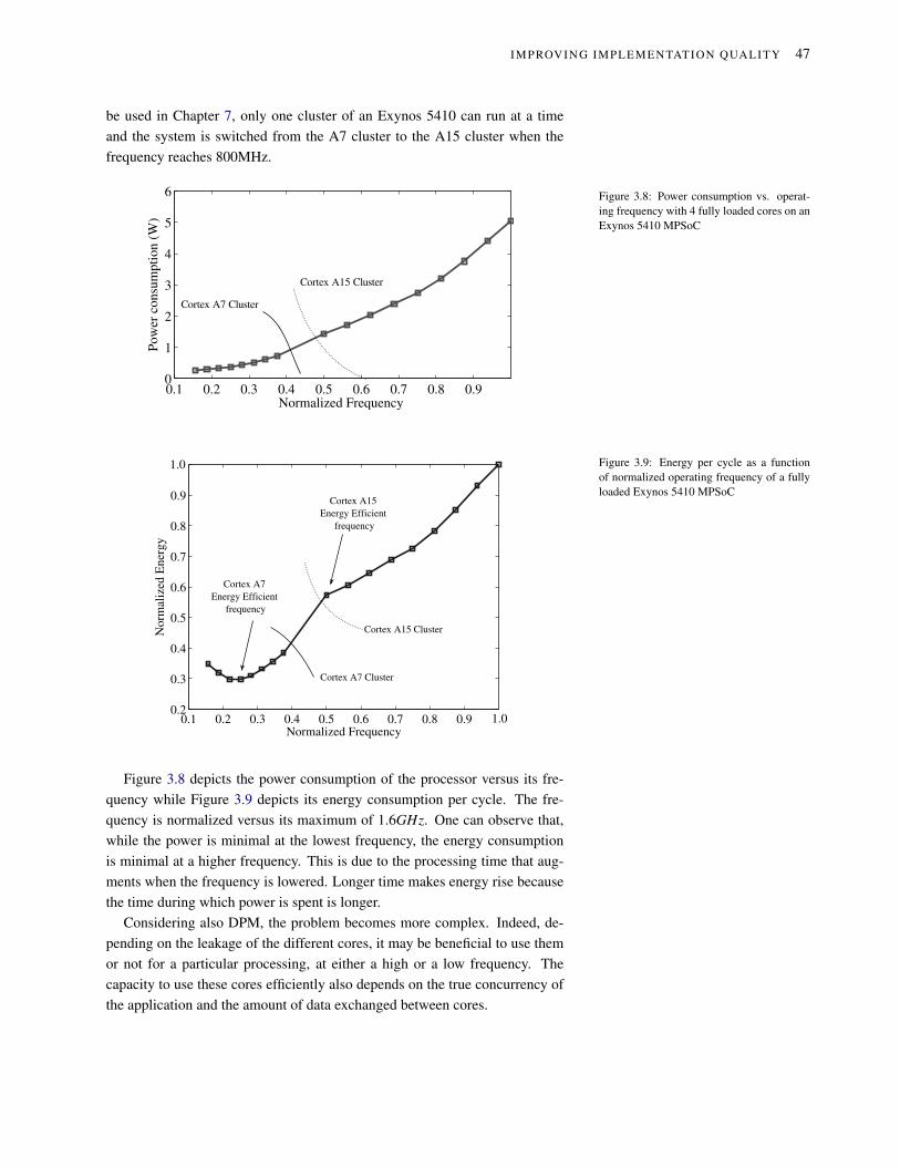
I MPROVIN G I MPLEMENTATION QUA LITY 47
be used in Chapter 7, only one cluster of an Exynos 5410 can run at a time
and the system is switched from the A7 cluster to the A15 cluster when the
frequency reaches 800MHz.
0.1 0.2 0.3 0.4 0.5 0.6 0.7 0.8 0.90
1
2
3
4
5
6
Normalized Frequency
Pow
erco
nsu
mpti
on
(W)
Cortex A15 Cluster
Cortex A7 Cluster
Figure 3.8: Power consumption vs. operat-
ing frequency with 4 fully loaded cores on an
Exynos 5410 MPSoC
0.1 0.2 0.3 0.4 0.5 0.6 0.7 0.8 0.90.2
0.3
0.4
0.5
0.6
0.7
0.8
0.9
1.0
Normalized Frequency
Norm
alized
Energy
1.0
Cortex A7
Energy Efficient
frequency
Cortex A15 Cluster
Cortex A7 Cluster
Cortex A15
Energy Efficient
frequency
Figure 3.9: Energy per cycle as a function
of normalized operating frequency of a fully
loaded Exynos 5410 MPSoC
Figure 3.8 depicts the power consumption of the processor versus its fre-
quency while Figure 3.9 depicts its energy consumption per cycle. The fre-
quency is normalized versus its maximum of 1.6GHz. One can observe that,
while the power is minimal at the lowest frequency, the energy consumption
is minimal at a higher frequency. This is due to the processing time that aug-
ments when the frequency is lowered. Longer time makes energy rise because
the time during which power is spent is longer.
Considering also DPM, the problem becomes more complex. Indeed, de-
pending on the leakage of the different cores, it may be beneficial to use them
or not for a particular processing, at either a high or a low frequency. The
capacity to use these cores efficiently also depends on the true concurrency of
the application and the amount of data exchanged between cores.

48 MODELS , METHODS AND TOOLS FO R BR IDG ING THE DESI GN PRO DUCTI VI TY GAP OF EMBEDDED
SIG NAL PROCESSI NG SY STEMS
From a static dataflow representation of a pipeline shaped application, con-
vex programming is used in Erwan Nogues PhD thesis to choose, for each
actor, the most optimal frequency and number of operating cores on a complex
MPSoC11. The result is non-trivial and the most optimal operating point de- 11 Erwan Nogues. Energy optimization of Sig-
nal Processing on MPSoCs and its Applica-
tion to Video Decoding. PhD thesis, INSA de
Rennes, 2016
pends much on the amount of concurrency of the application and the energetic
behaviour of the platform.
in outactor 2
outactor 1
in outactor 3 actor 4
in
w1 = 115e6 w2 = 1.15e6 w3 = 460e6 w4 = 23.03e6
1 1 1 11 1
Figure 3.10: example of a simple dataflow
application to be optimize in energy over an
MPSoC with DVFS and DPM capabilities.
Figure 3.10 shows a single-rate SDF application with static loads expressed
in numbers of cycles. 4 iterations of the applications are assumed to be exe-
cutable in parallel. Potential execution strategies for this application are illus-
trated in 3.11, 3.12 and 3.13.
core
time
frequency
deadline
actor 1.2
out
actor 1.1
out
actor 1.1
out
actor 1.1
out
actor 2.4
out
actor 2.3
out
actor 2.2
out
actor 2.1
outin
actor 3.4
out
actor 3.3
out
actor 3.2
out
actor 3.1
outin
actor 4.4
actor 4.3
actor 4.2
actor 4.1
in
Figure 3.11: As-fast-as-possible execution
of the application from Figure 3.10 on an
MPSoC with DVFS and DPM capabilities.
out
out
out
out
actor 1.1
actor 1.2
actor 1.3
actor 1.4
core
time
frequencydeadline
actor 2.3
actor 2.4
actor 2.1
actor 2.2
in
in
in
in out
out
out
out
in
out
out
out
outactor 3.3
actor 3.4
actor 3.2
actor 3.1actor 4.3
actor 4.4
actor 4.1
actor 4.2
in
in
in
in
Figure 3.12: As-slow-as-possible execution
of the application from Figure 3.10 on an
MPSoC with DVFS and DPM capabilities.
Figure 3.11 illustrates the case where the application 4 iterations are run
over a 4-core platform with maximum frequency and parallelism. This strat-
egy is called As-Fast-As-Possible (AFAP). Figure 3.12 illustrates the case,

I MPROVIN G I MPLEMENTATION QUA LITY 49
out
out
out
out
in
actor 1.1
actor 1.2
actor 1.3
actor 1.4
in
inout
in
in
in
actor 2.1
actor 2.2actor 3
actor 4.1
actor 4.2
actor 4.3
core
time
frequency
deadline
out
out
Figure 3.13: Most energy-efficient execu-
tion of application from Figure 3.10 on an
MPSoC with DVFS and DPM capabilities.
called As-Slow-As-Possible (ASAP), where the frequency is lowered as much
as possible while still respecting the application deadline. Energetic models
of an MPSoC platform are used to demonstrate that the most energy optimal
solution is neither as-fast-as-possible not As-slow-as-possible but rather a tai-
lored solution where some actors are forced to run on a limited number of
cores and different frequencies are set depending on the actor[53]. Energy
gains between 5% and 34% have been reported versus AFAP and ASAP on
synthetic benchmarks by using Geometric Programming (GP)[54] to find the
most energy optimal solution.
These results show the positive impact of exploiting the information of a
dataflow MoC for energy reduction. They open new opportunities for model-
based energy optimizations. These opportunities will be discussed in the con-
cluding Chapter 8.
The energy consumption studies of Erwan Nogues have been applied to
MPEG HEVC embedded decoding12. In the current PhD thesis of Alexandre 12 Erwan Nogues, Julien Heulot, Glenn Her-
rou, Ladislas Robin, Maxime Pelcat, Daniel
Menard, Erwan Raffin, and Wassim Hami-
douche. Efficient DVFS for low power
HEVC software decoder. Journal of Real-
Time Image Processing, 2016. Springer Ver-
lag
Mercat, we are starting a new study of the complexity and energy consump-
tion of an embedded HEVC encoder. The encoder is more computationally
intensive than the decoder13 and an encoder must test many possible encod-
13 Alexandre Mercat, Wassim Hamidouche,
Maxime Pelcat, and Daniel Menard. Estimat-
ing encoding complexity of a real-time em-
bedded software hevc codec. In Proceedings
of the DASIP conference. IEEE, 2016
ing methods for choosing the most optimal configuration in terms of bitrate and
image quality. In this context, energy is gained by smartly reducing the amount
of tested encoding methods14. This gain has an impact on the performance of
14 Alexandre Mercat, Florian Arrestier, Was-
sim Hamidouche, Maxime Pelcat, and Daniel
Menard. Energy reduction opportunities in an
hevc real-time encoder. In Proceedings of the
ICASSP conference, 2017
the encoder and this impact must be precisely controlled for the optimisations
to be useful in practice15. Such a system behavior where the functional behav-
15 Alexandre Mercat, Florian Arrestier, Was-
sim Hamidouche, Maxime Pelcat, and Daniel
Menard. Constrain the docile ctus: an in-
frame complexity allocator for hevc intra en-
coders. In Proceedings of the ICASSP con-
ference, 2017
ior, and non only NFPs, is affected by implementation optimizations goes out
of the scope of Design Productivity as defined in Chapter 1. It opens to the
domain of Approximate Computing that will be evoked in Chapter 8.
3.5 Conclusions on Implementation Quality
This chapter has focused on the gains obtained by using dataflow MoCs on the
processing memory consumption and the energy consumption of an MPSoC.
One important point to note is that our methods and tools have been created to
automate these gains. As a consequence, the developed approaches make low

50 MODELS , METHODS AND TOOLS FO R BR IDG ING THE DESI GN PRO DUCTI VI TY GAP OF EMBEDDED
SIG NAL PROCESSI NG SY STEMS
memory and low energy attainable without additional effort for the designer.
This element makes our studies impact DP through implementation quality.
The next section studies the use cases and protocol we developed to assess
DP in its different modalities.

4
Evaluating Design Productivity
DP
?Figure 4.1: Evaluating Design Productivity.
4.1 Chapter Abstract
Two elements are essential for measuring the productivity of a DSP system
design procedure. Use case systems must be built in realistic conditions and
these use cases should be representative of the DSP systems targeted by the
evaluated set of models, methods and tools. Moreover, a fair protocol must
be adopted to ensure that the benefits offered by the new design process are
not overrated or underrated. In this chapter, we first overview the use cases
we built in the last years to evaluate design processes. Then, a protocol is pro-
posed for fair DP evaluation and this protocol is demonstrated on an example.
Design Productivity (DP) is a multi-faceted concept and the amount of DP
observed for a given design depends on the experience of designers, on the
amount of constraints on implementation quality, on the time-to-market, etc.
As a consequence, building reliable DP comparisons between several design
methods is a delicate operation that requires a precise protocol and an equal
treatment of the compared design methods. However, DP evaluation is impor-
tant for assessing the maturity of design tools, evaluate the user-friendliness
of a language or check the appropriateness of a design method.
This chapter demonstrates the fair DP assessment protocol on an HLS com-
piler compared to the synthesis of manually written VHDL code. The choices of
Non-Functional Properties (NFPs) and Non-Recurring Engineerings (NREs)
costs for measuring respectively the implementation quality and the design ef-
ficiency are discussed. Experimental results are generated from the evaluation
of the CAPH HLS compiler and the reasons that make CAPH higher level than
VHDL are discussed.
4.2 Building DSP Use Cases for Testing Design Meth-
ods
Precise and complex use cases are needed to test “in vivo” new system de-
sign procedures in terms of both design efficiency and implementation quality.

52 MODELS , METHODS AND TOOLS FO R BR IDG ING THE DESI GN PRO DUCTI VI TY GAP OF EMBEDDED
SIG NAL PROCESSI NG SY STEMS
We have developed over the years a set of challenging use case designs and
published on the obtained performances. These use case applications belong
to the technical fields of telecommunications, cryptology, computer vision,
video compression, medical imaging, and artificial intelligence. From these
use cases, we analyse the difficulties of automating design and the causes of
DP losses. The next section exemplifies this effort on the use case of a 4G base
station algorithm modeling with PiSDF1. 1 Karol Desnos. Memory Study and Dataflow
Representations for Rapid Prototyping of
Signal Processing Applications on MPSoCs.
PhD thesis, INSA Rennes, 20144.2.1 A 4G Telecommunication Use Case: the LTE PUSCH
3GPP Long Term Evolution (LTE), which commercially corresponds to the
fourth generation of mobile telecommunications (4G), is a wireless telecom-
munication standard released in 2009. A complete method to describe a 4G
base station with a dataflow MoC is presented in our book 2. 2 Maxime Pelcat, Slaheddine Aridhi,
Jonathan Piat, and Jean-François Nezan.
Physical Layer Multi-Core Prototyping: A
Dataflow-Based Approach for LTE eNodeB.
Springer, 2012
Figure 4.2 presents a PiSDF specification of the bit processing algorithm of
the Uplink Physical Layer data processing (PUSCH) decoding which is part
of LTE. LTE PUSCH decoding is executed once per millisecond in the phys-
ical layer of an LTE base station. An LTE base station manipulates the data
of the hundreds of User Equipments (UEs) (for instance mobile phones) lo-
cated in its geographical region composed of “cells”. It consists of receiving
multiplexed data from several UEs, decoding and demultiplexing the data, and
transmitting it to upper Open Systems Interconnection (OSI) layers of the LTE
standard. This procedure is complex and computationally intensive. The in-
formation is received on several antenna at the base station side and time and
frequency multiplexed using Single-Carrier Frequency Division Multiple Ac-
cess (SC-FDMA).
ConfigNbCB
ConfigNbUE NbUE
ConvergeNbCB: NbUE
Symbols: maxCBsPerUE*NbUE
mac
sym
bols
snk
PUSCH Bit Processing
Symbols: maxCBsPerUE
NbCB: 1
NbCB
KeepCurrentTones
NbC
BS
ymbo
ls
PerUEProcess.
BitProcess.
TurboDec.
CRCCheck
snk
Symbols: NbCBSymbols: maxCBsPerUE
CBs: NbCBCB: 1
CB: 1CBs: NbCB
Channel Decoding
CB: 1
maxCBsPerUE
ChannelDecoding
Figure 4.2: PiSDF Model of the Bit Process-
ing Part of the LTE PUSCH Decoding
Because the number of UEs connected to a base station and the data rate

EVALUATING DESIG N PRO DUCTI VITY 53
received from each UE can change every millisecond, the bit processing of
PUSCH decoding is inherently dynamic and cannot be modeled with static
MoCs such as SDF [11]. The PUSCH bit processing specification can be mod-
eled by two hierarchical actors: the PUSCH Bit Processing actor and the Chan-
nel Decoding actor. For clarity, Figure 4.2 shows a simplified specification of
the LTE PUSCH decoding process where some actors and parameters are not
depicted.
The PUSCH Bit Processing actor is executed once per invocation of the
PUSCH decoding process (i.e. once per millisecond) and has a static pa-
rameter, maxCBsPerUE, that represents the maximum number of data blocks
(named Code Block (CB)) received per UE. maxCBsPerUE statically sets the
configuration input interface of the lower level of the hierarchy, according to
the base station limitation of bitrate for a single UE. The ConfigNbUE configu-
ration actor consumes data tokens coming from the upper OSI Medium Access
Control (MAC) layer and sets the configurable parameter NbUE representing
the number of UEs whose data must be decoded in the current millisecond.
The converge actor consumes the multiplexed CBs received from the several
antennas of the base station on the symbols data input interface of the graph.
It produces NbUE tokens, each containing the number of CBs for one UE, and
produces NbUE packets of maxCBsPerUE CBs, each containing the CBs of a
UE.
The Channel Decoding hierarchical actor fires NbUE times, once for each
UE, because each UE has specific signal channel conditions and thus a specific
channel decoding procedure. This actor has a configuration input interface
maxCBsPerUE that receives the eponymous locally static parameter from the
upper hierarchy level. The ConfigNbCB configuration actor sets the NbCB
parameter with the number of CBs allocated for the current UE.
The numbers of UEs and CBs can both reach 100. The number of potential
application configurations is thus very high [11]. This example illustrates how
a very dynamic applications can be modeled with PiSDF.
4.2.2 Other Modeled DSP Use Cases
In the cryptology domain, we have studied a cryptographic algorithm based on
chaos theory 3. We have used the memory and parallelism analysis offered by
3 Karol Desnos, Safwan El Assad, Aurore Ar-
licot, Maxime Pelcat, and Daniel Menard.
Efficient multicore implementation of an
advanced generator of discrete chaotic se-
quences. In Proceedings of the ICITST con-
ference, pages 31–36. IEEE, 2014
PiSDF to provide details on the performance of a cryptographic key generator.
In the image processing domain, we recently explored a dimensionality re-
duction algorithm for hyperspectral images 4. This algorithm is used to choose
4 Raquel Lazcano, Daniel Madroñal, Karol
Desnos, Maxime Pelcat, Raúl Guerra, Se-
bastián López, Eduardo Juarez, and César
Sanz. Parallelism Exploitation of a Dimen-
sionality Reduction Algorithm Applied to
Hyperspectral Images. In Proceedings of the
DASIP Conference, 2016
among a very large number of spectral bands the few spectral bands that con-
tain the most information. It uses Principal Component Analysis (PCA) and
represents a challenging use case due to large processed data. The algorithm is
ported to a many-core MPPA processor from Kalray and applied to detecting
brain cancer cells from hyperspectral images taken live during a brain opera-
tion.

54 MODELS , METHODS AND TOOLS FO R BR IDG ING THE DESI GN PRO DUCTI VI TY GAP OF EMBEDDED
SIG NAL PROCESSI NG SY STEMS
The MPEG HEVC encoder 5 and decoder 6,7 are some of our preferred use 5 Alexandre Mercat, Wassim Hamidouche,
Maxime Pelcat, and Daniel Menard. Estimat-
ing encoding complexity of a real-time em-
bedded software hevc codec. In Proceedings
of the DASIP conference. IEEE, 20166 Erwan Raffin, Erwan Nogues, Wassim
Hamidouche, Seppo Tomperi, Maxime Pel-
cat, and Daniel Menard. Low power hevc
software decoder for mobile devices. Jour-
nal of Real-Time Image Processing, 20167 Carlo Sau, Francesca Palumbo, Maxime
Pelcat, Julien Heulot, Erwan Nogues, Daniel
Ménard, Paolo Meloni, and Luigi Raffo.
Challenging the best HEVC fractional pixel
FPGA interpolators with reconfigurable and
multi-frequency approximate computing.
IEEE Embedded Systems Letters, 2017.
IEEE, to appear
cases, video compression being one of the main specialties of the VAADER
team from IETR. As an example,an algorithm from the HEVC standard is used
in the next sections to illustrate the creation of a DP evaluation procedure.
We are also extensively using a computer stereo vision matching algorithm8
8 Jinglin Zhang, Jean-Francois Nezan,
Maxime Pelcat, and Jean-Gabriel Cousin.
Real-time gpu-based local stereo matching
method. In Proceedings of the DASIP
Conference. IEEE, 2013
for our DP studies. This algorithm will be used in Chapter 7 to evaluate the
learning procedure of a Model of Architecture (MoA) from platform measure-
ments.
We are starting in the PhD thesis of Kamel Abdelouahab to address deep
learning use cases based on Convolutional Neural Networks (CNNs) 9. CNNs
9 Kamel Abdelouahab, Cédric Bourrasset,
Maxime Pelcat, François Berry, Jean-Charles
Quinton, and Jocelyn Serot. A holistic ap-
proach for optimizing dsp block utilization of
a cnn implementation on fpga. In Proceed-
ings of the ICDSC Conference. ACM, 2016
are exponentially gaining interest because of their demonstrated ability to per-
form image and video recognition and natural language processing with un-
precedented performances. Their regular structure and data locality make them
particularly well suited to dataflow-based methods.
Finally, the undergoing PhD thesis of Jonathan Bonnard and and El Mehdi
Abdali both study the hardware implementation of computer vision algorithms
in the objective of porting them to smart cameras.
The next section exposes on one use case our proposed protocol for evalu-
ating DP.
4.3 Introducing a Design Productivity Evaluation Pro-
tocol
The rest of this chapter describes a protocol for measuring the DP of a method
when compared to a reference. In order to make the study more concrete
and create the protocol, an HEVC video compression use case is implemented
and an HLS method is compared to writing VHDL manually for building an
FPGA-based system. We first introduce the notion of HLS before analyzing
the protocol and its results. This protocol has been published in the Proceed-
ings of IC-SAMOS 201610. 10 Maxime Pelcat, Cédric Bourrasset, Luca
Maggiani, and François Berry. Design pro-
ductivity of a high level synthesis compiler
versus HDL. In Proceedings of IC-SAMOS,
20164.3.1 HLS as a Tool for Improving Hardware Design DP
The most commonly used languages for Electronic Design Automation (EDA)
logic synthesis today are the VHDL, Verilog and SystemVerilog Hardware
description languages (HDLs). HDL languages are used to describe a hard-
ware implementation at a Register Transfer Level (RTL), i.e. at a level where
an implementation is constructed from signal transfers between registers and
from logical and arithmetic operations applied to these signals. However, this
domination of HDL languages is currently regressing and High-Level Synthe-
sis (HLS) methods are becoming market practice in the industry [65]. An HLS
method raises the level of abstraction of the code manipulated by designers
higher than RTL and replaces the VHDL or Verilog entry languages by a soft-
ware language such as plain C code, often accompanied by additional informa-

EVALUATING DESIG N PRO DUCTI VITY 55
tions such as pragmas. HLS methods ambition to improve design efficiency
while maintaining solid implementation Quality of Results (QoR).
In this chapter, we use HLS as a use case for testing our DP measurement
method. The scope of this HLS DP study is illustrated in Figure 4.3 as the first
step of the design process and before compilation, optimization and place &
route.
Optimized netlist(Gate level)
Netlist(Gate level)
VHDL files(RTL level)
HLS entry(High level)
Place & RoutePhysicalDevice
High-Level Synthesis
Synthesis Optimization
Compilation
Simulation
Simulation
Scope of the Study
Figure 4.3: Scope of the HLS versus VHDL
DP study.
The main motivation behind HLS is to improve the DP of hardware design-
ers by providing some correct-by-construction features and by separating the
correctness design concern from the timing design concern. This separation of
concerns is provided by a design process consisting of three steps:
1. the HLS compiler is fed with an untimed description of the algorithm. Us-
ing a timeless test bench, the correctness of the produced output values can
be checked regardless of their arrival time,
2. RTL code is generated either in VHDL or in Verilog from the higher level
language, and the correct arrival time of the output signals is checked,
3. additional constraints can be set on the RTL code generator to correct po-
tential violations of time and resource constraints.
Depending on the HLS method, different high-level descriptions are used
such as the imperative C and C++ languages and their extensions SystemC and
OpenCL, or the BlueSpec functional language [66]. Dataflow based descrip-
tions, built over the DPN paradigm [13] like the models introduced in Chap-
ter 2, are an alternative to classical HLS methods where the input language
does not follow an imperative paradigm.
While imperative languages decompose a computation into a sequence of
successive operations (similarly to an algorithmic description), dataflow lan-
guages decompose a computation into actors communicating only via FIFOs.
A drawback of using a dataflow language when compared to C/C++ or Sys-
temC code is that a less common programming paradigm, close to the func-
tional programming paradigm, must be learned by the designer. However,

56 MODELS , METHODS AND TOOLS FO R BR IDG ING THE DESI GN PRO DUCTI VI TY GAP OF EMBEDDED
SIG NAL PROCESSI NG SY STEMS
whereas parallelism must be inferred from code analysis in imperative HLS,
parallelism is naturally present in a dataflow algorithm description. Dataflow
languages for HLS exist both in academia (e.g. CAL [67] and CAPH [68]) and
in the industry (e.g. Cx [69]). The DPN paradigm is specifically suited to sig-
nal processing problems where limited control is necessary and computation
should be triggered by data availability. For that reason, we use a dataflow-
based language in this chapter to build our DP evaluation protocol for DSP
systems.
The following study does not intend to promote a particular HLS language
or method or to display advanced quality metrics on a given FPGA. Instead, a
precise and reproducible procedure is defined for assessing DP. While difficult,
this task is fundamental to drive the future developments of design methods.
The application chosen for applying the method is the MPEG HEVC [70]
interpolation filter. This 2-dimensional separable FIR filter is a simple yet
costly operation that requires fine implementation tuning. Moreover, the con-
volutions composing this filter are canonical examples of signal processing.
The HLS system chosen for evaluating DP assessment is the CAPH dataflow
compiler, compiling the CAPH language [68]. CAPH is a dataflow language
based on a functional paradigm.
4.3.2 Choosing NFPs and NREs Metrics and Designing the Pro-
tocol
As stated in Chapter 1, the DP of a design method is a trade-off between an
implementation quality to optimize, expressed as a set of NFPs (frequency,
area, memory, etc.) and design efficiency expressed as NRE costs.
The objective of the study is to produce DP radar charts equivalent to the
ones in Figure 1.1 and also a DP metric representative of the tested method
performance.
The obtained radar charts for the use case are displayed later in Figure 4.7.
We introduce 3 metrics to assess DP: the gain in NRE design time GNRE eval-
uating design efficiency, the quality loss LQ evaluating implementation quality
and finally the design productivity PD evaluating the trade-off between design
quality and design efficiency. These metrics are then computed on the use case
and lead to the results presented in Section 4.3.8.
Choosing the NREs Metrics to Evaluate Design Efficiency Design efficiency
results from a combination of parameters including the complexity of the de-
sign under development, the amount of NRE tasks to execute (i.e. the cost of
the new code to produce), the expressiveness, and “developer friendliness” of
the design languages, the available legacy code, the designer’s experience, the
testability of the results, the simulation time (influencing the time of design
and verification steps), and the maturity of the design tools.
Quantitative quality metrics can be computed to characterize both the tested

EVALUATING DESIG N PRO DUCTI VITY 57
HLS and reference HDL methods. System development time can be divided
into:
— 1.a NRE design time, i.e. time necessary for writing the code of a function-
ality,
— 1.b NRE verification time, i.e. time used for building a testbench and unit
testing,
— 1.c the system integration time, i.e. time necessary to build from compo-
nents a system respecting its requirements.
The system integration time, comprising verification and validation, de-
pends on features that go beyond DSP system design (analog to digital con-
version, energy management, physical environment, etc.). Reducing integra-
tion time by an HLS method would require a system completely defined with
the HLS method, including for example I/O drivers. The system tested in this
chapter, like all systems using HLS today, integrates HLS generated blocks
within a framework written with standard HDL. Integration time is thus con-
sidered out of the scope of this study.
Design times are controversial because they depend on the designer’s ex-
perience. Different times may be required for a design by a junior hardware
designer and a senior hardware designer. Software developers may themselves
require a different time. The design time is not systematically reproducible
(who has never experienced losing a few hours on a simple bug and its non-
explicit bug report?). Moreover, design time can not really be weighted by
an “experience rate” — an experienced designer is likely to spend more time
in unit testing and commenting, in order to save time in code integration and
training of colleagues. This study intends to overcome these difficulties by
comparing HDL and HLS in the same conditions. In the experiments, design
times measured for HDL and HLS reflect the time required by a single devel-
oper experienced on software signal processing but novice in both VHDL and
HLS languages. The experiments reflect the capacity of HLS to offer a high-
level API to a novice designer. This choice is consistent with the important
objective of HLS to open hardware design to a broader public of developers. A
selection of the time taken into account in measurements reduces the subjectiv-
ity of the approach. The time taken to refer to books and chapters for syntactic
details is excluded from the measured time. The development times are thus
sums of short design and verification times with a quantum of 1’ (minute) and
an average length of 15’.
Code properties complement the timing results:
— 2.a number of Source Lines Of Code (SLOC) (excluding blank lines and
comments),
— 2.b number of characters in the code (excluding blank lines and com-
ments).

58 MODELS , METHODS AND TOOLS FO R BR IDG ING THE DESI GN PRO DUCTI VI TY GAP OF EMBEDDED
SIG NAL PROCESSI NG SY STEMS
These grades reflect the complexity and expressiveness of the languages.
A lower number of lines in the HLS code than in the HDL code reflects the
abstraction of some implementation concerns. These numbers do not fully
reflest complexity, as for instance, one line of regular expression may have a
greater complexity than 20 lines of C code. As a consequence, SLOCs are not
used in the DP metric but rather as an additional information.
Choosing the NFP Metrics to Evaluate Implementation Quality The NFPs
Metrics depend on the chosen hardware platform. In this study, we choose as
a target a Field-Programmable Gate Array (FPGA). On an FPGA implemen-
tation, quality metrics are divided into area and time information. We propose
the following metrics:
— 3.a number of Lookup tables (LUTs)
— 3.b number of registers,
— 3.c number of Random Access Memory (RAM) blocks,
— 3.d number of DSP cores.
— 4.a processing latency,
— 4.b minimum operating period.
Computing a Metric for Design Productivity As HLS aims at reducing design
time, the gain in global NRE time GNRE is the most important metric of design
efficiency. GNRE is defined formally as:
GNRE =tHDLdesign + tHDL
veri f
tHLSdesign + tHLS
veri f
(4.1)
where tHDLdesign and tHDL
veri f are respectively the design and verification times when
writing the application in HDL. Similarly, tHLSdesign and tHLS
veri f are the design and
verification times when writing the application in HLS. A time gain GNRE
greater than 1 reflects the ability of an HLS method to save design and/or ver-
ification time. If only design and verification times are evaluated to assess an
HLS method, methods resulting in a fast design with low quality are favored.
In the proposed method, a quality degradation metric is included that penalizes
low quality systems.
Implementation quality metrics depend on the constraints of the design
(strict frequency constraint, strong resource limitations...). To take into ac-
count in a single cost the different quality metrics constituting a QoR vector,
the implementation cost is defined as the weighted sum of normalized features
to minimize [71]. The normalization of the different hardware quality met-
rics is done with respect to the maximum amount on the chosen system. For

EVALUATING DESIG N PRO DUCTI VITY 59
instance, the maximum period of the design obtained with HDL is computed
as:
prdHDLnorm = prdHDL/prdsystem
max , (4.2)
where prdsystemmax is the maximum period for supporting the application (for in-
stance, to ensure the frame rate). In the general case of HLS DP measurement,
we define quality loss as:
LQ =∑φHLS
i ∈ΦHLS αi × (φ HLSi )
∑φHDLi ∈ΦHDL αi × (φ HDL
i ), (4.3)
where ΦHLS is the sets of normalized quality metrics to minimize and αi are
normalizing coefficients. In particular, in the case of an FPGA, we can define
quality loss as:
LQ =α1 × lutHLS
norm +α2 × regHLSnorm +α3 × ramHLS
norm+
α1 × lutHDLnorm +α2 × regHDL
norm +α3 × ramHDLnorm+
α4 ×dspHLSnorm +α5 × latHLS
norm +α6 × prdHLSnorm
α4 ×dspHDLnorm +α5 × latHDL
norm +α6 × prdHDLnorm
(4.4)
where lutHDLnorm and lutHLS
norm are numbers of LUTs (3.a), regHDLnorm and regHLS
norm are
numbers of registers (3.b), ramHDLnorm and ramHLS
norm are numbers of RAM blocks
(3.c), dspHDLnorm and dspHLS
norm are numbers of DSP blocks (3.d), latHDLnorm and latHLS
norm
are latencies (4.a), and prdHDLnorm and prdHLS
norm are operating periods (4.b).
The parameters αi can be tuned to favor different hardware features. We
propose 2 approaches: 1) architecture-relative where each al phai is set to 1,
and 2) fair to place all metrics on an equal footing, where each (non null) pair
of values is normalized to its maximum:
αi =
0, if max(φ HLSi ,φ HDL
i ) = 0.
(max(φ HLSi ,φ HDL
i ))−1, otherwise.(4.5)
for φ HLSi ∈ Φ
HLS and φ HDLi ∈ Φ
HDL. The architecture-relative approach is
specific to a single device because it favors metrics that are sparse on the
measured platform. Experimental results (Section 4.3.8) focus on the fair ap-
proach, putting all parameters on the same footing.
Quality loss LQ reflects the loss due to rising the level of abstraction. A low
LQ reflects a good HLS generated code quality. We introduce the HLS Design
Productivity (DP) metric as a unique grade to assess the trade-off between
design efficiency and quality. System DP ratio is defined as:
PD = GNRE /LQ (4.6)
A new design method can be considered successful if its DP is greater than
1. Two design methods can be compared in terms of DP, provided that the
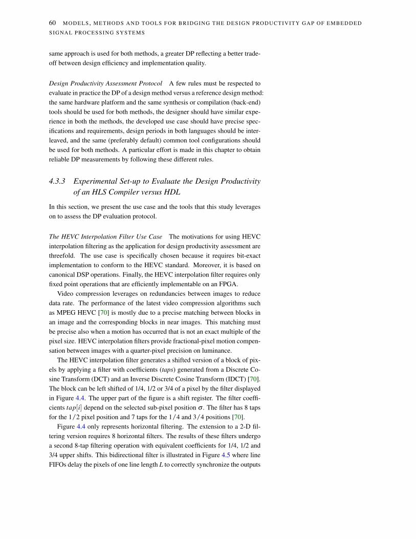
60 MODELS , METHODS AND TOOLS FO R BR IDG ING THE DESI GN PRO DUCTI VI TY GAP OF EMBEDDED
SIG NAL PROCESSI NG SY STEMS
same approach is used for both methods, a greater DP reflecting a better trade-
off between design efficiency and implementation quality.
Design Productivity Assessment Protocol A few rules must be respected to
evaluate in practice the DP of a design method versus a reference design method:
the same hardware platform and the same synthesis or compilation (back-end)
tools should be used for both methods, the designer should have similar expe-
rience in both the methods, the developed use case should have precise spec-
ifications and requirements, design periods in both languages should be inter-
leaved, and the same (preferably default) common tool configurations should
be used for both methods. A particular effort is made in this chapter to obtain
reliable DP measurements by following these different rules.
4.3.3 Experimental Set-up to Evaluate the Design Productivity
of an HLS Compiler versus HDL
In this section, we present the use case and the tools that this study leverages
on to assess the DP evaluation protocol.
The HEVC Interpolation Filter Use Case The motivations for using HEVC
interpolation filtering as the application for design productivity assessment are
threefold. The use case is specifically chosen because it requires bit-exact
implementation to conform to the HEVC standard. Moreover, it is based on
canonical DSP operations. Finally, the HEVC interpolation filter requires only
fixed point operations that are efficiently implementable on an FPGA.
Video compression leverages on redundancies between images to reduce
data rate. The performance of the latest video compression algorithms such
as MPEG HEVC [70] is mostly due to a precise matching between blocks in
an image and the corresponding blocks in near images. This matching must
be precise also when a motion has occurred that is not an exact multiple of the
pixel size. HEVC interpolation filters provide fractional-pixel motion compen-
sation between images with a quarter-pixel precision on luminance.
The HEVC interpolation filter generates a shifted version of a block of pix-
els by applying a filter with coefficients (taps) generated from a Discrete Co-
sine Transform (DCT) and an Inverse Discrete Cosine Transform (IDCT) [70].
The block can be left shifted of 1/4, 1/2 or 3/4 of a pixel by the filter displayed
in Figure 4.4. The upper part of the figure is a shift register. The filter coeffi-
cients tap[i] depend on the selected sub-pixel position σ . The filter has 8 taps
for the 1/2 pixel position and 7 taps for the 1/4 and 3/4 positions [70].
Figure 4.4 only represents horizontal filtering. The extension to a 2-D fil-
tering version requires 8 horizontal filters. The results of these filters undergo
a second 8-tap filtering operation with equivalent coefficients for 1/4, 1/2 and
3/4 upper shifts. This bidirectional filter is illustrated in Figure 4.5 where line
FIFOs delay the pixels of one line length L to correctly synchronize the outputs

EVALUATING DESIG N PRO DUCTI VITY 61
x[t]
tap[7]tap[6]
x[t-1]
tap[5]
x[t-2]
tap[4]
x[t-3]
tap[3]
x[t-4]
tap[2]
x[t-5]
tap[1]
x[t-6]
tap[0]
x[t-7]
y[t-7]
8
16 16 16 16 16 16 16 16
8 888888
16
/6410
clip88
horizontal filterinput pixel flow
filtered pixel flow
Figure 4.4: Signal flow of an HEVC interpo-
lation filter for horizontal shift of 1/4, 1/2 or
3/4 of a pixel.
of the different horizontal filters.
horizontal filter
horizontal filter
horizontal filter
horizontal filter
horizontal filter
horizontal filter
inputpixelflow picture line FIFO
x[t]
x[t-L]
x[t-2L]
x[t-3L]
x[t-4L]
x[t-5L]
x[t-6L]
x[t-7L]
8
16
16
16
16
16
16
horizontal filter
horizontal filter 16
16
22
22
22
22
22
22
22
22
22/642
10
clip8
8
filteredpixelflow
y[t-7L-7]
tap[0]
tap[1]
tap[2]
tap[3]
tap[4]
tap[5]
tap[6]
tap[7]
Figure 4.5: Signal flow of a 2-dimensional
HEVC interpolation filter for horizontal and
vertical shift of 1/4, 1/2 or 3/4 of a pixel.
The use case being normative, data sizing is derived from the standard spec-
ifications. This is an important point because it limits the design choices and
helps comparing different versions of the code. The presented filters corre-
spond to the core of the luminance filters. In the next sections, the presented
filters serve as the basis for the HLS vs. HDL study.
Used Design Tools and Platform The software tools and versions used for
the study are:
• Altera Quartus II versions 13.1.0.162 and VHDL 2008,
• Mentor Graphics Modelsim ASE, delivered with Quartus,
• CAPH Compiler version 2.7.0.
A golden reference of the filter Design Under Test (DUT) is coded in C
language. This implementation is out of the scope of the study and serves
for verifying both the HDL and the HLS implementations. The HDL code is

62 MODELS , METHODS AND TOOLS FO R BR IDG ING THE DESI GN PRO DUCTI VI TY GAP OF EMBEDDED
SIG NAL PROCESSI NG SY STEMS
ported to an FPGA-based smart camera named DreamCAM [72]. This camera
embeds an Altera Cyclone III EP3C120F780C7N FPGA. Using a camera aims
at making the study close to designer’s best practices by not limiting the study
to simulations. A complex pattern of data valid signals makes the filter not
trivial to port on the camera.
4.3.4 Designing HEVC Interpolation Filters in VHDL
In this section, the use case is implemented in HDL and qualitative as well as
quantitative elements are given on the design effort. VHDL [73] is a language
for hardware description standardized in 1987 and revised in 1993, 2000, 2002,
and 2008. A VHDL program consists of explaining how a digital circuit is
structured and what the behavior of each component is. These behaviors can
be purely combinatorial, sequential or more commonly mixed.
Assumptions and Verification of the Use Case Design The number of possible
designs in HDL for a filter such as the ones presented in Section 4.3.3 is large.
Accesses to external memory to store intermediate values can alter much the
quality. It is also possible to use existing Intellectual Property core (IP) blocks
or “design templates” (especially for FIR filters). The choice of parallelizing
or sequencing operations is also very important.
In order to narrow the design space, some assumptions are taken on the
input and output pixel streams of our use case. The filter is synchronous to
a unique clock and has asynchronous reset. The input pixel stream comes
in raster order (i.e. scanning the image from left to right and from top to
bottom) in a stream of 8-bit pixels. A data valid signal states whether the
current clock corresponds to a data value. Each filter configuration (1/4, 1/2
or 3/4 horizontal and vertical shifts) is studied independently and coefficients
are considered constant. In an HEVC encoder or decoder, the filter must then
be duplicated for the different positions. A sufficient number of clock events
without data is given for the filter to resume execution at the end of a pixel
line. The last assumption is compatible with most CMOS image sensors that
provide horizontal and vertical blanking. The assumptions foster a pipelined
design with FIFOs such as the ones illustrated in Figures 4.4 and 4.5. Several
versions of the filter are designed with their test benches. A golden reference
code in C language provides reference values for debug.
VHDL Version 1: Horizontal Filter with Minimal Interfaces In this version
of the filter, implementing the diagram in Figure 4.4, the stream of input pixels
is considered continuous (1 clock event = 1 data). A transition to zero of the
data valid signal resets the filter. It is interpreted as the beginning of a new
line and thus, the filter needs to gather 8 data before outputting the first valid
data. Based on the writing of this HDL filter, the time needed to describe the
pipelined quarter pixel filter in HDL is 358’ for design and 288’ for verifica-

EVALUATING DESIG N PRO DUCTI VITY 63
tion, including time for writing the test bench, RTL simulation, and debug.
The algorithm description time includes all the reflections on the description
(data types, generics, sizing, the use of functions, data conversions, use of best
practices...) and the writing, from scratch, of the VHDL files.
VHDL Version 2: Horizontal Filter with Interfaces for the DreamCAM Cam-
era When porting the filter onto the camera, the VHDL block must input and
output a data valid signal (indicating pixel validity for each clock event) as
well as a frame valid signal. The frame valid signal is continuously set during
the reception of a frame and reset at the end of the frame. Clock events that do
not carry data happen pseudo randomly during the reception of an image.
The time needed to describe the filter in HDL is 162’ for design and 783’ for
debug, including 152’ on a test bench and 631’ on the DreamCAM platform.
VHDL Version 2 shows that porting an algorithm onto a real platform has a
large cost, even when the algorithm has already passed some RTL verification
process.
VHDL Version 3: 2-D Filter with Interfaces for the DreamCAM Camera This
filter is designed by reusing the VHDL version 2 horizontal filter and combin-
ing filter results of several lines such as in Figure 4.5. The time needed to
describe the filter in HDL is 232’ for design and 775’ for verification.
The main difficulties comes again from the control part of the filter that
determines when a data is valid or not and on which cycle it must appear on
a given signal. In particular, synchronizing data valid and frame valid sig-
nals have necessitated most of the time. Next section discusses the sources of
VHDL non-optimality in terms of design productivity that make room for HLS
methods.
4.3.5 Discussion on the Origins of VDHL Complexity
The Counterpart of VHDL Versatility In order to build verifiable logic, it is
recommended to design a fully synchronous system. Using VHDL, a designer
is however free to design asynchronous circuits and gated clocks that are chal-
lenging to verify. For instance, while rarely being necessary, latch constructs
may be generated by mistake with VHDL, for instance with an incomplete
IF T HEN ELSE statement in a combinatorial process. Latches are strongly
discouraged in literature [73] and this type of “low level implementation bugs”
is at the heart of the need for HLS methods [66].
A Unique Language for Different Objectives A difficulty of VHDL comes
from the combination, in a single language, of simulation-oriented and implementation-
oriented features. For example, operators such as modulus MOD or remainder
REM are generally not synthesizable [73].

64 MODELS , METHODS AND TOOLS FO R BR IDG ING THE DESI GN PRO DUCTI VI TY GAP OF EMBEDDED
SIG NAL PROCESSI NG SY STEMS
Some Unintuitive Properties The absence of precedence in logical operators
makes the following expression:
y <= a and b or c and d
equivalent to:
y <= ((a and b) or c) and d.
This property stands in contradiction to the mathematical order of operation
and can cause errors that are difficult to detect for a new programmer.
The Historical Reasons Some difficulties of the VHDL language come from
the different techniques available to implement a single functionality. For in-
stance, an 8-bit unsigned integer signal data can be declared by
SIGNAL data : INTEGER RANGE 0 TO 255;
or by
SIGNAL data : UNSIGNED (7 DOWNTO 0);
Choosing between the two solutions requires a knowledge that is not related
to system design but rather to language implementation details. The integer
style is typically used to manipulate data within a design while the unsigned
style is used for designing I/Os.
The Fundamental Reason The main productivity limitation while using VHDL
is the tangle of value and timing concerns. A value is considered as correctly
received only if it arrives at an exact predefined clock event. During design, a
lot of time is spent to obtain a value one cycle later or, worse, one cycle sooner
than what the current design outputs. As an input signal of an entity must be
present when its corresponding valid signal occurs, much of the design time is
spent to synchronize data and control signals.
Now that VHDL design characteristics have been presented, next section
details for comparison the design of the same filter versions with the CAPH
HLS language.
4.3.6 Introduction to the CAPH Language
CAPH [68] is a domain-specific language (DSL) for describing and imple-
menting stream processing applications on configurable hardware, such as
FPGAs. CAPH was first released in 2011 and is based upon the dataflow model
of computation where an application is described as a network of autonomous
processing elements (actors) exchanging tokens through unidirectional chan-
nels (FIFOs).
As the CAPH language is not mainstream like the VHDL language, details
on the syntax and semantics are given in this section. The behavior of indi-
vidual actors in CAPH is specified using a set of transition rules, where a rule
consists of a set of patterns, involving inputs and local variables, and a set of
expressions, describing modifications of outputs and local variables. Tokens

EVALUATING DESIG N PRO DUCTI VITY 65
circulating on channels and manipulated by actors are either data tokens (car-
rying actual values, such as pixels for example) or control tokens (acting as
structuring delimiters). With this approach, fine grain processing (down to the
pixel level) is expressed without global control or synchronization.
As an example, the actor coded in Listing 4.1 computes the sum of a list
of values. Given the input stream < 1 2 3 > < 4 5 6 >, — where 1, 2,
. . . represent data tokens and < and > control tokens respectively encoding the
start and the end of a list — the CAPH program produces the values 6, 15.
For this, the CAPH code uses two local variables : An accumulator s and a
state variable st. st indicates whether the actor is actually processing a list or
waiting for a new list to start. In the first state, the accumulator keeps track of
the running sum. The first rule can be read as : when waiting for a list (st=S0)
and reading the start of a new one (i=’<), then reset accumulator (s:=0) and
start processing (st=S1). The second rule says : When processing (st=S1)
and reading a data value (i=’v), then update accumulator (s:=s+v). The last
rule is fired at the end of the list (i=’>); the final value of the accumulator
is written on output o. This style of description fits a stream-based execution
model where pixels are processed “on the fly”.
Listing 4.1: An actor computing the sum of values along lists in CAPH.
actor suml
in (i: signed<8> list)
out (o: signed<16>)
var st: {S0,S1}=S0
var s : signed<16>
rules
(st:S0, i:’<) -> (st:S1, s:0)
| (st:S1, i:’v) -> (st:S1, s:s+v)
| (st:S1, i:’>) -> (st:S0, o:s)
For describing the structure of dataflow graphs, CAPH embeds a textual
Network Description Language (NDL). NDL is a higher-order, purely func-
tional language in which dataflow graphs are described by defining and ap-
plying wiring functions. A wiring function is a function accepting and return-
ing wires (graph edges). This concept is illustrated in Figure 4.6, where the
dataflow graph on the left is described by the CAPH program on the right. In
this example, two wiring functions are defined : neigh13 and neigh33. The
former takes a wire and produces a bundle of three wires representing the 1×3
neighborhood of the input stream, by applying twice the one-pixel delay actor
dp. The latter takes a wire and produces a bundle of nine wires representing
the 3×3 neighborhood of the input stream, by applying the previously defined
neigh13 function and the dl actor (one-line delay)
The tool chain supporting the CAPH language comprises a reference inter-
preter and a compiler producing both SystemC and synthetizable, platform-
independent VHDL code. The SystemC back-end is used for verification.

66 MODELS , METHODS AND TOOLS FO R BR IDG ING THE DESI GN PRO DUCTI VI TY GAP OF EMBEDDED
SIG NAL PROCESSI NG SY STEMS
net neigh13(x) =
x,
dp x,
dp (dp x);
net neigh33(x) =
neigh13 x,
neigh13 (dl x),
neigh13 (dl (dl x));
net
(o11,o12,o13),
(o21,o22,o23),
(o31,o32,o33)
= neigh33(i);
DPDP
DL DP DP
DL DP DP
i
o11
o12
o13
o21
o22
o23
o31
o32
o33
Figure 4.6: Example of a graph description
in CAPH.
4.3.7 Writing the MPEG HEVC Interpolation Filters in CAPH
Assumptions and Verification of the Use Case Design The assumptions on
the filter are the same as in the VHDL description case: pixel flow in raster
order, unique clock, valid signal and sufficient blanking (Section 4.3.4).
Data validation is automated by the CAPH compiler based on the struc-
tural tokens < and > in the bitstream (Section 4.3.6). The CAPH environment
provides FIFOs implemented in VHDL that automate data valid management.
Moreover, a VHDL wrapper for the CAPH-generated VHDL code exists for
the DreamCAM camera, driving inputs and FIFOs with the data valid signals
of the camera. These features may appear unfair for the comparison between
VHDL and CAPH but, in our opinion, VHDL and CAPH are treated on an
equal footing, as they are both ported to the platform with tools helping the
connection of their communication means (signals in VHDL, FIFOs in CAPH)
to their environment (a CMOS sensor and a USB port).
CAPH Version 1: Horizontal Filter with Minimal Interfaces In version 1 of
the HEVC filter in CAPH, the code is composed of a single actor receiving
the image bitstream and sending the horizontally filtered data. The test bench
represents only 5 lines of code connecting the actor to the input and output
streams. This simple test bench is possible because the HLS compiler performs
only functional verification and time verification is left to the synthesizer. The
actor implements a shift register and a counter discards the 7 first output tokens
that do not represent valid data. The actor has four transition rules and most of
the design time is taken to find the right way to represent the shift register in
CAPH. In this version, the shift register is made of a set of internal variables in
the CAPH actor. The filter is functionally equivalent to its VHDL counterpart
after 103’ for design and 65’ for writing the test bench and debugging the filter
with a SystemC simulation.

EVALUATING DESIG N PRO DUCTI VITY 67
CAPH Version 2: Horizontal Filter with Interfaces for the DreamCAM Cam-
era Similarly to its VHDL counterpart, this version 2 of the filter in CAPH is
adapted to the DreamCAM needs, resetting the filter at the end of each line and
adding modularity to the description. The filter is decomposed into 8 pipelined
multiply-accumulate actors. The last actor in the pipeline has a different code.
It gathers the intermediate products into a filtered and clipped value and gen-
erates the output flow. The main difficulty comes from getting rid of unwanted
tokens, i.e. tokens that appear while the pipeline is filled up and emptied. The
time for designing this version, composed of 9 actors, can be decomposed into
71’ for design and 72’ for verification.
CAPH Version 3: 2-D Filter In this 2-D version of the filter, 7 new delay
actors are first instantiated and connected. CAPH higher order functions are
used to create a large number of actors with a code of limited size. Delay actors
insert L first dummy tokens in the stream, where L is the length of a picture line,
and then forward the arriving pixel values. The time needed to describe the
2-D filter in CAPH is split into 187’ for design and 169’ for verification.
4.3.8 Experimental Results: Evaluating the Design Productivity
of the CAPH HLS Compiler versus VHDL
Overview of the Experimental Results Table 4.1 summarizes the experimen-
tal results of the different versions of the use case and Figure 4.7 illustrates
them. Concerning CAPH results, values reported in brackets correspond to the
total hardware resources including the overhead of the transformation from the
platform signals (frame and data valid) to the token representation. These num-
bers are the fairest to compare to VHDL so they are the ones used for quality
assessment.
VHDL CAPH VHDL CAPH VHDL CAPH
v1 v1 v2 v2 v3 v3
NREdesign (minutes) 358 103 162 71 232 187
NREveri f (minutes) 288 65 783 72 775 169
# SLOCs 147 43 333 61 805 194
# chars 4114 1351 9465 2395 22072 6099
# LUTs 193 226 282 3161 2868 11398
(445) (3380) (11636)# Regs 81 103 115 2209 1252 7557
(269) (2375) (7723)# RAM 0 0 (1) 0 0 (1) 18 14
Frequency (MHz) 64.7 68.0 71.8 83.0 65.2 84.2
Table 4.1: VHDL vs. CAPH design effi-
ciency and implementation quality figures.
Figure 4.7 displays values normalized to the largest of the two values. One
can see that HLS is obtaining gains on design efficiency because, in the upper
part of the charts, the CAPH values are smaller than the VHDL values (smaller
is better). Conversely, there is a quality loss due to HLS that makes the VHDL
values smaller than the CAPH values in the lower part of the chart. The CAPH

68 MODELS , METHODS AND TOOLS FO R BR IDG ING THE DESI GN PRO DUCTI VI TY GAP OF EMBEDDED
SIG NAL PROCESSI NG SY STEMS
HLS method is efficient for frequency; it even obtains slightly better mini-
mum period than manual VHDL. This effect can be explained by the insula-
tion of each actors by FIFOs that build a pipeline. However, CAPH presents
a large overhead in terms of LUTs and registers. This effect is explained by
the automatic insertion of FIFO queues between actors that are not present in
VHDL (VHDL). Improving the footprint of the VHDL generated from CAPH
is thus an important objective to make this HLS method competitive. Globally,
a smaller area in the clear red zone than in the dark blue zone is a good indica-
tor that HLS is reaching a higher DP than VHDL; this fact will be confirmed
in the next sections.
NREdesign
NREveri f
SLOC
LUTs
Regs
prd
(a) v1
NREdesign
NREveri f
SLOC
LUTs
Regs
prd
(b) v2
NREdesign
NREveri f
SLOC
RAM
LUTs Regs
prd
(c) v3
Figure 4.7: Design efficiency and implemen-
tation quality chart (the smaller the better) for
each filter in CAPH (clear red) and VHDL
(dark blue).Gain in NRE Design Time of CAPH vs. Manual VHDL Table 4.2 shows
for each use case version the Gain in NRE Design Time GNRE introduced in
Section 4.3.2. In average, designing the use case versions with the CAPH HLS
method took 4.42× less time than writing and testing VHDL by hand. The
standard deviation is large (1.96). This fact shows that, depending on the code
type (raw 1-D filter, 1-D filter with control or 2-D filter), the gain in design
time varies.
CAPH vs. CAPH vs. CAPH vs. Average
VHDL v1 VHDL v2 VHDL v3
GNRE 3.84× 6.60× 2.82× 4.42×
LQ 1.70× 2.53× 1.47× 1.90×
PD 2.26× 2.61× 1.92× 2.26×
Table 4.2: Gain in NRE Design Time GNRE ,
Quality Loss LQ and Design Productivity PD
of CAPH vs. manual VHDL.
Quality Loss of CAPH vs. Manual VHDL The quality loss, defined in Section
4.3.2, is evaluated to study the productivity of the HLS method. We focus in
this chapter on the fair approach, putting all parameters on equal footing to
make results not very dependent on the type of FPGA so normalization to
maximum values is skipped and parameters αi are computed by equation 4.5.

EVALUATING DESIG N PRO DUCTI VITY 69
Numbers of DSPs and latency are ignored in quality loss computation (α4 =
0 and α5 = 0) because the use case does not generate multipliers and the la-
tency of a few cycles introduced by VHDL and CAPH is negligible when com-
pared to the latency of several picture lines, mandatory in the 2-D filter, so
latency does not reflect system quality.
Quality loss LQ figures are displayed in Table 4.2. They show that, when
putting all quality metrics on an equal footing, there is in average a quality loss
of about 2× due to using the CAPH HLS method when compared to VHDL
manual writing. The standard deviation of 0.6 is limited.
Design Productivity of CAPH HLS versus Manual HDL From the previously
computed gain in NRE design time and quality loss, we can derive the Design
Productivity PD for the different use case versions. The values of PD are shown
in Table 4.2. The HLS Design Productivity (DP) metric for the tested CAPH
compiler version 2.7.0 is 2.2×. This number is an evaluation of the gains
obtained by the HLS compiler. The small standard deviation of 0.34 between
the different versions is an encouraging sign of the relevance of the DP metric
evaluation method proposed in this chapter. Finally, one can see in Figure 4.1
that while verification takes in average 3× the time of design in VHDL, it takes
in average only 85% of the design time in CAPH.
4.4 Discussion on the Reduction of Complexity when
using CAPH HLS Instead of VHDL
More than numbers, this DP studies gives us some insights on what makes the
tested HLS method higher level than the reference.
A dataflow MoC abstracts two elements:
• time. Instead of reacting to clock events, actors react to the arrival of data
tokens,
• amount of data stored in FIFOs. The MoC assumes FIFOs of sufficient size
to store pending tokens.
These two abstractions make it possible a first verification of the process
independently from the notion of time. The designer can thus verify very early
in the design process whether the output values conform to the specification.
Moreover, by generating SystemC code for simulation and verification, the
CAPH compiler leverages on an optimized simulation environment. Writing
the test bench in CAPH is also fairly less complex than in VHDL.
These advantages come at the cost of a higher memory consumption, mostly
due to the allocation of FIFO queues between actors.

70 MODELS , METHODS AND TOOLS FO R BR IDG ING THE DESI GN PRO DUCTI VI TY GAP OF EMBEDDED
SIG NAL PROCESSI NG SY STEMS
4.5 Conclusion and Perspectives
In this chapter, our use cases and a protocol to assess DP gains have been
presented. Using this protocol, an HLS compiler based on the CAPH dataflow
programming language has been compared to manual VHDL.
The framework for design productivity estimation proposed in this chap-
ter can be extended to any type of software and hardware system design.
Figures of merit for the implementation quality and design efficiency should
be adapted to the system under test. However, the method and recommen-
dations remain valid. Crossbreeding different design methods and combining
their best features in a unique method could offer new opportunities of DP
enhancement for complex heterogeneous system design.
Assessing and comparing systems at a higher level of abstraction that the
RTL level used in this chapter is possible if cross-hardware Non-Functional
Properties (NFPs) are chosen to represent implementation performance. For
instance, if silicon area instead of LUTs is measured to estimate resource
needs, an FPGA can be compared to a multicore processor. Predicting such
high-level NFPs is the role of MoAs that will be developed in the second Part
of this document. The fairness of DP comparisons comes at the price of op-
timisation efforts both for the reference and tested methods and of a precise
protocol for evaluating design efficiency and implementation performance. To
the extent of our knowledge, the protocol presented in this chapter is the first
fair protocol for assessing DP. As new levels of abstractions appear for system
design and as model-based methods are increasingly adopted, fair DP assess-
ment becomes essential to better understand where efficiency lies and which
features bring a substantial productivity gain.
Our work of the last years has concentrated on DP improvements from ap-
plications modeled with dataflow MoCs. However, having information on the
platform architecture is crucial to automate the design of complex systems and
the body of work on architecture modeling is much more reduced than the one
on application modeling. The next sections of Part B detail a new research sub-
ject I wish to further investigate in the next years to provide this architectural
information: Models of Architecture.

Part B
Introducing MoAs for Raising Design
Productivity


5
Models of Architecture: A New Design Abstrac-
tion Model of Architecture
Application
Map
Architecture
NFPs
Redesign
Redesign
Figure 5.1: MoAs in the Y-chart.
5.1 Chapter Abstract
This chapter initiates the second part of this report that introduces and posi-
tions in state-of-the-art the new concept of Models of Architecture (MoAs) to
complement the work on MoCs and further improve the DP of DSP embedded
systems.
This chapter precisely defines the MoA concept that aims at representing
platform architectures at a high level of abstraction with the objective of feed-
ing efficient Design Space Exploration methods and, in turn, enhance design
productivity by automating some design decisions. MoAs formalize the archi-
tecture input of the Y-chart design approach in the same way MoCs formal-
ize the application input. The application/architecture separation of concerns
should not be confused with the hardware/software separation of concerns.
While the former is a fundamental model-related notion, the second is a tool-
related notion that tends to fade away with the adoption of virtualization and
HLS.
To be an MoA, an architecture model must respect three constraints: 1)
offer a reproducible cost computation for a Non-Functional Property (NFP)
when combined with an application model respecting a precise MoC, 2) be
application independent, and 3) abstract the computed cost. An architecture
model respecting only a subset of these rules is referred to as a quasi-MoA.
This chapter also introduces the notion of application activity that serves as
an intermediate between application and architecture models. Indeed, the NFP
cost (e.g. energy consumption) results from the activity of the application sup-
ported by the hardware platform.
In order to make the MoA concept more concrete, this chapter also in-
troduces a first MoA named Linear System-Level Architecture Model (LSLA).
LSLA computes an abstract NFP cost as a linear combination of the computa-

74 MODELS , METHODS AND TOOLS FO R BR IDG ING THE DESI GN PRO DUCTI VI TY GAP OF EMBEDDED
SIG NAL PROCESSI NG SY STEMS
tion and communication tokens composing application activity. LSLA will be
compared to state-of-the-art architecture description languages and models in
Chapter 6 and its capacities will be demonstrated in Chapter 7.
5.2 The Context of Models of Architecture
5.2.1 Models of Architecture in the Y-Chart Approach
The main motivation for developing Models of Architecture is for them to
formalize the specification of an architecture in a Y-chart approach of system
design. The Y-chart approach, introduced in [74], consists in separating in two
independent models the application-related and architecture-related concerns
of a system’s design.
Model of Architecture
Model ofComputation Application
Mapper and Simulator
efficiency metrics
conform to conform to
redesign redesign
What How
Architecture
Figure 5.2: MoC and MoA in the Y-chart.
This concept is refined in Figure 5.2 where a set of applications is mapped
to a set of architectures to obtain a set of efficiency metrics. In Figure 5.2,
the application model is required to conform to a specified MoC and the ar-
chitecture model is required to conform to a specified MoA. This approach
aims at separating What is implemented from How it is implemented. In this
context, the application is qualified by a Quality of Service (QoS) and the ar-
chitecture, offering resources to this application, is characterized by a given
efficiency when supporting the application. For the discussion not to remain
abstract, next section illustrates the problem on an example.
5.2.2 Illustrating Iterative Design Process and Y-Chart on an
Example System
QoS and efficiency metrics are multi-dimensional and can take many forms.
For a signal processing application, QoS may be the Signal-to-Noise Ratio
(SNR) or the Bit Error Rate (BER) of a transmission system, the compression
rate of an encoding application, the detection precision of a radar, etc. In terms
of architectural decisions, the obtained set of efficiency metrics is composed
of some of the following Non-Functional Properties (NFPs):
• over time:

MODELS O F ARCH ITECTU RE : A N EW D ESIGN ABSTRACTIO N 75
– latency (also called response time) corresponds to the time duration be-
tween the arrival time of data to process and the production time of pro-
cessed data,
– throughput is the amount of processed data per time iterval,
– jitter is the difference between maximal and minimal latency over time,
• over energy consumption:
– energy corresponds to the energy consumed to process an amount of
data,
– peak power is the maximal instantaneous power required on alimentation
to process data,
– temperature is the effect of dissipated heat from processing,
• over memory:
– RAM requirements corresponds to the amount of necessary read-write
memory to support processing,
– Read-Only Memory (ROM) requirements is the amount of necessary read-
only memory to support processing,
• over security:
– reliability is 1− p f with p f the probability of system failure over time,
– electromagnetic interference corresponds to the amount of non-desired
emitted radiations,
• over space:
– area is the total surface of semiconductor required for a given process-
ing,
– volume corresponds to the total volume of the built system.
– weight corresponds to the total weight of the built system.
• and cost corresponds to the monetary cost of building one system unit under
the assumption of a number of produced units.
When compared to the implementation efficiency metrics developed in Sec-
tion 4.3.2, these system efficiency metrics are more generic, architecture-independent
and application-related. They make it possible to compare software-defined
and hardware-defined systems by observing the NFPs of a “black-box” sys-
tem.
The high complexity of automating system design with a Y-chart approach
comes from the extensive freedom (and imagination) of engineers in redesign-
ing both application and architecture to fit the efficiency metrics, among this

76 MODELS , METHODS AND TOOLS FO R BR IDG ING THE DESI GN PRO DUCTI VI TY GAP OF EMBEDDED
SIG NAL PROCESSI NG SY STEMS
list, falling into their applicative constraints. Figure 5.3 is an illustrating ex-
ample of this freedom on the application side. Let us consider a video com-
pression system to be ported on a platform. As shown in Figure 5.3 a), the
application initially has only pipeline parallelism. Assuming that all four tasks
are equivallent in complexity and that they receive and send at once a full im-
age as a message, pipelining can be used to map the application to a multicore
processor with 4 cores, with the objective to rise throughput (in frames per
second) when compared to a monocore execution. However, latency will not
be reduced because data will have to traverse all tasks before being output. In
Figure 5.3 b), the image has been split into two halves and each half is pro-
cessed independently. The application QoS in this second case will be lower,
as the redundancy between image halves is not used for compression. The
compression rate or image quality will thus be degraded. However, by accept-
ing QoS reduction, the designer has created data parallelism that offers new
opportunities for latency reduction, as processing an image half will be faster
than processing a whole image.
colorprocessing
predictiontransform &quantization
entropycoding
colorprocessing
predictiontransform &quantization
entropycoding
colorprocessing
predictiontransform &quantization
entropycoding
compressedbitstream 1
compressedbitstream 2
a) original video compression application
b) redesigned video compression application forcing data parallelism
Figure 5.3: Illustrating designer’s freedom on
the application side with a video compression
example.
In terms of architecture, and depending on money and design time resources,
the designer may chose to run some tasks in hardware and some in software
over processors. He can also choose between different hardware intercon-
nects to connect these architecture components. For illustrative purpose, Fig-
ure 5.4 shows different configurations of processors that could run the appli-
cations of Figure 5.3. rounded rectangles represent Processing Elements (PEs)
performing computation while ovals represent Communication Nodes (CNs)
performing inter-PE communication. Different combinations of processors
are displayed, leveraging on high-performance out-of-order ARM Cortex-A15
cores, on high-efficiency in-order ARM Cortex-A7 cores, on the Multi-Format
Codec (MFC) hardware accelerator for video encoding and decoding, or on
Texas Instruments C66x Digital Signal Processing cores. Figure 5.4 g) cor-
responds to a 66AK2L06 Multicore DSP+ARM KeyStone II processor from
Texas Instruments where ARM Cortex-A15 cores are combined with C66x
cores connected with a Multicore Shared Memory Controller (MSMC) [75].
In these examples, all PEs of a given type communicate via shared memory

MODELS O F ARCH ITECTU RE : A N EW D ESIGN ABSTRACTIO N 77
with either hardware cache coherency (Shared L2) or software cache coherency
MSMC), and with each other using either the Texas Instruments TeraNet switch
fabric or the ARM AXI Coherency Extensions (ACE) with hardware cache co-
herency [76].
ARMCortexA7
ARMCortexA7
ARMCortexA7
ARMCortexA7
SharedL2
ARMCortexA15
ARMCortexA15
ARMCortexA15
ARMCortexA15
SharedL2
ACE
ARMCortexA7
ARMCortexA7
ARMCortexA7
ARMCortexA7
SharedL2
MFCACE
ARMCortexA7
a) monocoreenergy-efficient
ARMCortexA15
b) monocorehigh-performance ARM
CortexA7ARM
CortexA7
ARMCortexA7
ARMCortexA7
SharedL2
c) quad-core energy-efficient
e) quad-core energy-efficient + accelerator f) octo-core big.LITTLE
ARMCortexA15
ARMCortexA15
ARMCortexA15
ARMCortexA15
SharedL2
c) quad-core high-performance
ARMCortexA15
ARMCortexA15
SharedL2
TIC66x
TIC66x
TIC66x
TIC66x
MSMCTeraNet
g) multi-ARM + multi-DSP processor from Texas Instruments
Figure 5.4: Illustrating designer’s freedom
on the architecture side with some current
ARM-based and Digital Signal Processor-
based multi-core architectures.
Each architecture configuration and each mapping and scheduling of the
application onto the architecture leads to different efficiencies in all the previ-
ously listed NFPs. Considering only one mapping per application-architecture
couple, models from Figures 5.3 and 5.4 already define 2× 7 = 14 systems.
Adding mapping choices of tasks to PEs, and considering that they all can
execute any of the tasks and ignoring the order of task executions, the num-
ber of possible system efficiency points in the Pareto Chart is already roughly
19.000.000. This example shows how, by modeling application and archi-
tecture independently, a large number of potential systems is generated which
makes automated multi-dimensional DSE necessary to fully explore the design
space.
5.2.3 On the separation between application and architecture
concerns
Separation between application and architectural concerns should not be con-
fused with software (SW) / hardware (HW) separation of concerns. The soft-
ware/hardware separation of concerns is often put forward in the term HW/SW
co-design. Software and its languages are not necessarily architecture-agnostic
representations of an application and may integrate architecture-oriented fea-
tures if the performance is at stake. This is shown for instance by the differ-
ences existing between the C++ and CUDA languages. While C++ builds an
imperative, object-oriented code for a processor with a rather centralized in-
struction decoding and execution, CUDA is tailored to GPGPUs with a large

78 MODELS , METHODS AND TOOLS FO R BR IDG ING THE DESI GN PRO DUCTI VI TY GAP OF EMBEDDED
SIG NAL PROCESSI NG SY STEMS
set of cores. As a rule of thumb, software qualifies what may be reconfigured
in a system while hardware qualifies the static part of the system.
The separation between application and architecture is very different in the
sense that the application may be transformed into software processes and
threads, as well as into hardware IPs. Software and Hardware application parts
may collaborate for a common applicative goal. In the context of Digital Signal
Processing (DSP), this goal is to transform, record, detect or synthetize a signal
with a given QoS. MoCs follow the objective of making an application model
agnostic of the architectural choices and of the HW/SW separation. The ar-
chitecture concern relates to the set of hardware and software support features
that are not specific to the DSP process, but create the resources supporting the
application.
On the application side, many MoCs have been designed to represent the
behavior of a system. The Ptolemy II project [77] has a considerable influence
in promoting MoCs with precise semantics. Different families of MoCs exist
such as finite state machines, process networks, Petri nets, synchronous MoCs
and functional MoCs. This chapter defines MoAs as the architectural counter-
parts of MoCs and presents a state-of-the-art on architecture modeling for DSP
systems.
5.2.4 Scope of this Part B
In this Part B, we focus on architecture modeling for the performance estima-
tion of a DSP application over a complex distributed execution platform. We
keep functional testing of a system out of the scope of the chapter and rather
discuss the early evaluation of system non-functional properties. As a con-
sequence, virtual platforms such as QEMU [78], gem5 [79] or Open Virtual
Platforms simulator (OVPsim), that have been created as functional emulators
to validate software when silicon is not available, will not be discussed. MoAs
work at a higher level of abstraction where functional simulation is not central.
The concept of MoA has been introduced in1. 1 Maxime Pelcat, Karol Desnos, Luca
Maggiani, Yanzhou Liu, Julien Heulot,
Jean-François Nezan, and Shuvra S
Bhattacharyya. Models of architecture:
Reproducible efficiency evaluation for signal
processing systems. In Proceedings of the
SiPS Workshop. IEEE, 2016
The considered systems being dedicated to digital signal processing, the
study concentrates on signal-dominated systems where control is limited and
provided together with data. Such systems are called transformational, as
opposed to reactive systems that can, at any time, react to non-data-carrying
events by executing tasks.
Finally, the focus is put on system-level models and design rather than on
detailed hardware design, already addressed by large sets of existing literature.
Next section introduces the concept of an MoA, as well as an MoA example
named Linear System-Level Architecture Model (LSLA).

MODELS O F ARCH ITECTU RE : A N EW D ESIGN ABSTRACTIO N 79
5.3 The Model of Architecture Concept
The concept of MoA is evoked in 2002 in [80] where it is defined as “a formal
representation of the operational semantics of networks of functional blocks
describing architectures”. This definition is broad, and allows the concepts
of MoC and MoA to overlap. As an example, a SDF graph [16] represent-
ing a system fully specialized to an application may be considered as a MoC,
because it formalizes the application. It may also be considered as an MoA
because it fully complies with the definition from [80]. The Definition 4 of
this chapter is a new definition [2] of an MoA that does not overlap with the
concept of MoC. The LSLA model is then presented to clarify the concept by
an example.
5.3.1 Definition of an MoA
Prior to defining MoA, the notion of application activity is introduced that en-
sures the separation of MoC and MoA. Figure 5.5 illustrates how application
activity provides intermediation between application and architecture. Appli-
cation activity models the computational burden supported by the architecture
when executing the application.
Application modelMoC
Architecture modelMoA
applicationactivity
abstractefficiencycost
activity tokenactivity quantum
data data
efficiencycost
fixingphysical
unit
Figure 5.5: Application activity as an inter-
mediate model between application and ar-
chitecture.
Definition 1 Application activity A corresponds to the amount of process-
ing and communication necessary for accomplishing the requirements of the
considered application during the considered time slot. Application activity is
composed of processing and communication tokens, themselves composed of
quanta.
Definition 2 A quantum q is the smallest unit of application activity. There
are two types of quanta: processing quantum qP and communication quantum
qC.
Two distinct processing quanta are equivalent, thus represent the same amount
of activity. Processing and communication quanta do not share the same unit
of measurement. As an example, in a system with a unique clock and byte-
addressable memory, 1 cycle of processing can be chosen as the processing
quantum and 1 byte as the communication quantum.

80 MODELS , METHODS AND TOOLS FO R BR IDG ING THE DESI GN PRO DUCTI VI TY GAP OF EMBEDDED
SIG NAL PROCESSI NG SY STEMS
Definition 3 A token τ ∈ TP∪TC is a non-divisible unit of application activity,
composed of a number of quanta. The function size : TP ∪TC → N associates
to each token the number of quanta composing the token. There are two types
of tokens: processing tokens τP ∈ TP and communication tokens τC ∈ TC.
The activity A of an application is composed of the set:
A = {TP,TC} (5.1)
where TP = {τ1P,τ2
P,τ3P...} is the set of processing tokens composing the appli-
cation processing and TC = {τ1C,τ2
C,τ3C...} is the set of communication tokens
composing the application communication.
An example of a processing token is a run-to-completion task with always
identical computation. All tokens representing the execution of this task en-
close the same number N of processing quanta (e.g. N cycles). An example of
a communication token is a message in a message-passing system. The token
is then composed of M communication quanta (e.g. M Bytes). Using the two
levels of granularity of a token and a quantum, an MoA can reflect the cost
of managing a quantum, and the overhead of managing a token composed of
several quanta.
Definition 4 A Model of Architecture (MoA) is an abstract efficiency model of
a system architecture that provides a unique, reproducible cost computation,
unequivocally assessing an architecture efficiency cost when supporting the
activity of an application described with a specified MoC.
This definition makes three aspects fundamental for an MoA:
• reproducibility: using twice the same MoC and activity computation with a
given MoA, system simulation should return the exact same efficiency cost,
• application independence: the MoC alone carries application information
and the MoA should not comprise application-related information such as
the exchanged data formats, the task representations, the input data or the
considered time slot for application observation. Application activity is an
intermediate model between a MoC and an MoA that prevents both models
to intertwine. An application activity model reflects the processing burden
to be supported by architecture and should be versatile enough to support a
large set of MoCs and MoAs, as demonstrated in [2].
• abstraction: a system efficiency cost, as returned by an MoA, is not bound
to a physical unit. The physical unit is associated to an efficiency cost out-
side the scope of the MoA. This is necessary not to redefine the same model
again and again for energy, area, weight, etc.
Definition 4 does not compel an MoA to match the internal structure of the
hardware architecture, as long as the generated cost is of interest. An MoA for

MODELS O F ARCH ITECTU RE : A N EW D ESIGN ABSTRACTIO N 81
energy modeling can for instance be a set of algebraic equations relating appli-
cation activity to the energy consumption of a platform. To keep a reasonably
large scope, this chapter concentrates on graphical MoAs defined hereafter:
Definition 5 A graphical MoA is an MoA that represents an architecture with
a graph Λ = 〈M,L, t, p〉 where M is a set of “black-box” components and
L ⊆ M×M is a set of links between these components.
The graph Λ is associated with two functions t and p. The type function
t : M × L 7→ T associates a type t ∈ T to each component and to each link.
The type dedicates a component for a given service. The properties function
p : M×L×Λ 7→ P(P), where P represents powerset, gives a set of properties
pi ∈ P to each component, link, and to the graph Λ itself. Properties are
features that relate application activity to implementation efficiency.
When the concept of MoA is evoked throughout this chapter, a graphical
MoA is supposed, respecting Definition 5. When a model of a system ar-
chitecture is evoked that only partially compels with this definition, the term
quasi-MoA is used, equivalent to quasi-moa in [2] and defined hereafter:
Definition 6 A quasi-MoA is a model respecting some of the aspects of Defi-
nition 4 of an MoA but violating at least one of the three fundamental aspects
of an MoA, i.e. reproducibility, application independence, and abstraction.
All state-of-the-art languages and models presented in Sections 6.2 and 6.3
define quasi-MoAs. As an example of a graphical quasi-MoAs, the graphical
representation used in Figure 5.4 shows graphs Λ = 〈M,L〉 with two types of
components (PE and CN), and one type of undirected link. However, no infor-
mation is given on how to compute a cost when associating this representation
with an application representation. As a consequence, reproducibility is vio-
lated. Next section illustrates the concept of MoA through the LSLA example.
5.3.2 Example of an MoA: the Linear System-Level Architecture
Model (LSLA)
The LSLA model computes an additive reproducible cost from a minimalistic
representation of an architecture [2]. As a consequence, LSLA fully complies
with Definition 5 of a graphical MoA. The LSLA composing elements are
illustrated in Figure 5.6. An LSLA model specifies two types of components:
Processing Elements and Communication Nodes, and one type of link. LSLA
is categorized as linear because the computed cost is a linear combination of
the costs of its components.
Definition 7 The Linear System-Level Architecture Model (LSLA) is a Model
of Architecture (MoA) that consists of an undirected graph Λ= (P,C,L,cost,λ )
where:

82 MODELS , METHODS AND TOOLS FO R BR IDG ING THE DESI GN PRO DUCTI VI TY GAP OF EMBEDDED
SIG NAL PROCESSI NG SY STEMS
Link
PE Processing Element
CN Communication Node
10s+1 Per token cost(s=size(token))
z
PE2
1s
x y
10s 1sPE110s+1
5s+1 PE4
PE3 2s+1
2s+1λ=0.3
Figure 5.6: LSLA MoA semantics elements.
• P is a set of Processing Elements (PEs). A PE is an abstract processing
facility with no assumption on internal parallelism, Instruction Set Archi-
tecture (ISA), or internal memory. A processing token τP from application
activity must be mapped to a PE p ∈ P to be executed.
• C is the set of architecture Communication Nodes (CNs). A communication
token τC must be mapped to a CN c ∈C to be executed.
• L = {(ni,n j)|ni ∈ C,n j ∈ C ∪ P} is a set of undirected links connecting
either two CNs or one CN and one PE. A link models the capacity of a CN
to communicate tokens to/from a PE or to/from another CN.
• cost is a property function associating a cost to different elements in the
model. The cost unit is specific to the non-functional property being mod-
eled. It may be in mJ for studying energy or in mm2 for studying area.
Formally, the generic unit is denoted ν .
On the example displayed in Figure 5.6, PE1−4 represent Processing Ele-
ments (PEs) while x, y and z are Communication Nodes (CNs). As an MoA,
LSLA provides reproducible cost computation when the activity A of an ap-
plication is mapped onto the architecture. The cost related to the management
of a token τ by a PE or a CN n is defined by:
cost : TP ∪TC ×P∪C → R
τ ,n 7→ αn.size(τ)+βn,
αn ∈ R,βn ∈ R
(5.2)
where αn is the fixed cost of a quantum when executed on n and βn is the
fixed overhead of a token when executed on n. For example, in an energy
modeling use case, αn and βn are respectively expressed in energy/quantum
and energy/token, as the cost unit ν represents energy. A token communicated
between two PEs connected with a chain of CNs Γ = {x,y,z...} is reproduced
card(Γ) times and each occurrence of the token is mapped to 1 element of
Γ. This procedure is illustrated in Figure 5.7. In figures representing LSLA
architectures, the size of a token size(τ) is abbreviated into s and the affine
equations near CNs and PEs (e.g. 10s + 1) represent the cost computation
related to Equation 5.2 with αn = 10 and βn = 1.
A token not communicated between two PEs, i.e. internal to one PE, does
not cause any cost. The cost of the execution of application activity A on an

MODELS O F ARCH ITECTU RE : A N EW D ESIGN ABSTRACTIO N 83
LSLA graph Λ is defined as:
cost(A ,Λ) = ∑τ∈TPcost(τ ,map(τ))+
λ ∑τ∈TCcost(τ ,map(τ))
(5.3)
where map : TP ∪TC → P∪C is a surjective function returning the mapping of
each token onto one of the architecture elements.
• λ ∈ R is a Lagrangian coefficient setting the Computation to Communica-
tion Cost Ratio (CCCR), i.e. the cost of a single communication quantum
relative to the cost of a single processing quantum.
Similarly to the SDF MoC [16], the LSLA MoA does not specify relations
to the outside world. There is no specific PEs type for communicating with
non-modeled parts of the system. This is in contrast with Architecture Analysis
and Design Language (AADL) processors and devices that separate I/O
components from processing components (Section 6.2.1). The Definition 1
of activity is sufficient to support LSLA and other types of additive MoAs.
Different forms of activities are likely to be necessary to define future MoAs.
Activity Definition 1 is generic to several families of MoCs, as demonstrated
in [2].
Figure 5.7 illustrates cost computation for a mapping of the video compres-
sion application shown in Figure 5.3 b), described with the SDF MoC onto the
big.LITTLE architecture of Figure 5.4 f), described with LSLA. The number
of tokens, quanta and the cost parameters are not representative of a real execu-
tion but set for illustrative purpose. The natural scope for the cost computation
of a couple (SDF, LSLA), provided that the SDF graph is consistent, is one
SDF graph iteration [2].
LSLA architecture
activity of an iteration:
2 colorProc tokens,
2 Pred tokens,
2 trans&Quant tokens,
2 entropyCod tokens,
1 mux&send token,
8 data tokens
SDF application
tokens relative costs:
decomposition into quanta.
mapping tokens to PEs and CNs.
communication tokens local from
one PE to the same PE are
discarded.λ=0.2
10s+1
10s+1 2s1s
3s+1
3s+1
predcolorProc1 1 trans&
Quant
1 1 1 1 1 2entropyCod
mux&send
ARM72
ARM73 1s
ARM71
ARM74
ARM152
ARM153
ARM151
ARM154
10s+1
10s+1
3s+1
3s+1
SL21 SL22ACE
consuming 2 tokens
and forcing 2 executions
of other actors
Figure 5.7: Computing cost of executing an
SDF graph on an LSLA architecture. The
cost for 1 iteration is (looking first at pro-
cessing tokens then at communication tokens
from left to right) 31+ 31+ 41+ 41+ 41+41+ 13+ 13+ 4+ 0.2× (5+ 5+ 5+ 10+5+ 5+ 10+ 5) = 266 ν (Equation 5.3).

84 MODELS , METHODS AND TOOLS FO R BR IDG ING THE DESI GN PRO DUCTI VI TY GAP OF EMBEDDED
SIG NAL PROCESSI NG SY STEMS
The SDF application graph has 5 actors colorProc, pred, trans&Quant,
entropyCod, and mux&Send and the 4 first actors will execute twice to pro-
duce the 2 image halves required by mux&Send. The LSLA architecture model
has 8 PEs ARM jk with j ∈ {7,15} and k ∈ {1,2,3,4}, and 3 CNs SL21, ACE
and SL22. Each actor execution during the studied graph iteration is trans-
formed into one processing token. Each dataflow token transmitted during one
iteration is transformed into one communication token. A token is embedding
several quanta (white squares), allowing a designer to describe heterogeneous
tokens to represent executions and messages of different weight.
In Figure 5.7, each execution of actors colorProc is associated with a cost
of 3 quanta and each execution of other actors is associated to a cost of 4 quanta
except mux&Send requiring 1 quantum. Communication tokens (representing
one half image transfer) are given 5 quanta each. These costs are arbitrary here
but should represent the relative computational burden of the task/communica-
tion.
Each processing token is mapped to one PE. Communication tokens are
“routed” to the CNs connecting their producer and consumer PEs. For in-
stance, the fifth and sixth communication tokens in Figure 5.7 are generating
3 tokens each mapped to SL21, ACE and SL22 because the data is carried from
ARM71 to ARM151. It is the responsibility of the mapping process to verify
that a link l ∈ L exists between the elements that constitute a communication
route. The resulting cost, computed from Equations 5.2 and 5.3, is 266ν . This
cost is reproducible and abstract, making LSLA an MoA.
5.4 What is New about MoAs?
LSLA is one example of an architecture model but many such models exist
in literature. Next chapter studies different languages and models from liter-
ature and explains the difference existing between an MoA fully respecting
Definition 4 and the quasi-MoAs state-of-the-art works define.

6
State of the Art of Models of Architecture
Figure 6.1: A common representation of 4
cores, a bus and a memory... without precise
semantics.
6.1 Chapter Abstract
This chapter positions the concept of Models of Architecture (MoAs) in state-
of-the-art languages and models for architecture description. This overview
will be published in the third edition of the Handbook of Signal Processing
Systems1. It covers three standard architecture modeling languages and four 1 Maxime Pelcat. Models of Architecture for
DSP Systems. In Shuvra S Bhattacharyya,
Ed F Deprettere, Rainer Leupers, and Jarmo
Takala, editors, Handbook of signal process-
ing systems, third edition. Springer Science
& Business Media, to appear, 2017
models from literature to help the understanding of previous work on MoAs.
All languages and models from literature are shown to define quasi-MoAs.
Indeed, none of the defined models respect the three MoA-defining constraints
specified in the previous chapter.
The AADL language is first studied and shown to define a quasi-MoA that
is reproducible but does not separate architectural concerns from application
concerns. Then, the quasi-MoA specified by the MCA SHIM standard language
is explained. It is tailored to the needs of multicore partitioning tools and
dedicated to time simulation. Finally, UML MARTE is demonstrated to specify
4 different quasi-MoAs with different simulation purposes. The computation of
NFPs from these quasi-MoAs is based on designer’s experience, which makes
reproducibility not guaranteed.
The evolution of formal architectural models is then presented with four
different models. These models have progressively introduced the notions of
system-level architecture abstraction, multi-dimensional exploration, internal
component parallelism and data transfer models. The notion of MoAs results
from this evolution and a property table gathering the properties of the dis-
cussed models is presented.
6.2 Architecture Design Languages and their Archi-
tecture Models
This section studies the architecture models provided by three standard Archi-
tecture Design Languages (ADLs) targeting architecture modeling at system-
level: AADL, MCA SHIM, and UML MARTE.

86 MODELS , METHODS AND TOOLS FO R BR IDG ING THE DESI GN PRO DUCTI VI TY GAP OF EMBEDDED
SIG NAL PROCESSI NG SY STEMS
While AADL adopts an abstraction/refinement approach where components
are first roughly modeled, then refined to lower levels of abstraction, UML
MARTE is closer to a Y-Chart approach where the application and the archi-
tecture are kept separated and application is mapped to architecture.
For its part, MCA SHIM describes an architecture with “black box” pro-
cessors and communications and puts focus on inter-PE communication simu-
lation. All these languages have in common the implicit definition of a quasi-
MoA (Definition 6). Indeed, while they define parts of graphical MoAs, none
of them respect the 3 rules of MoA Definition 4.
6.2.1 The AADL Quasi-MoA
Architecture Analysis and Design Language (AADL) [82] is a standard lan-
guage released by SAE International, an organization issuing standards for
the aerospace and automotive sectors. The AADL standard is referenced as
AS5506 [83] and the last released version is 2.2.
Some of the most active tools supporting AADL are Ocarina2 [84] and OS- 2 https://github.com/OpenAADL/ocarina
ATE3. 3 https://github.com/osate
AADL provides semantics to describe a software application, a hardware
platform, and their combination to form a system. AADL can be represented
graphically, serialized in XML or described in a textual language [85]. The
term architecture in AADL is used in its broadest sense, i.e. a whole made
up of clearly separated elements. A design is constructed by successive re-
finements, filling “black boxes” within the AADL context. Figure 6.2 shows
two refinement steps for a video compression system in a camera. Blocks of
processing are split based on the application decomposition of Figure 5.3 a).
First, the system is abstracted with external data entering a video compres-
sion abstract component. Then, 4 software processes are defined for the
processing. Finally, processes are transformed into 4 threads, mapped onto
2 processes. The platform is defined with 2 cores and a bus and application
threads are allocated onto platform components. The allocation of threads to
processors is not displayed. Sensor data is assigned a rate of 30 Hz, corre-
sponding to 30 frames per second. Next sections detail the semantics of the
displayed components.
Software, hardware and systems are described in AADL by a composition
of components. In this chapter, we focus on the hardware platform modeling
capabilities of AADL, composing an implicit graphical quasi-MoA. Partly re-
specting Definition 5, AADL represents platform with a graph Λ = 〈M,L, t, p〉
where M is a set of components, L is a set of links, t associates a type to each
component and link and p gives a set of properties to each component and link.
As displayed in Figure 6.3, AADL defines 6 types of platform components
with specific graphical representations. The AADL component type set is
such that t(c∈M)∈{system, processor, device, bus, memory, abstract}.
There is one type of link t(l ∈ L) ∈ {connection}. A connection can be set

STATE OF THE A RT OF MODELS OF ARC HITEC TURE 87
abstract systemvideo compression
video compression system
sensor_datacompressed_data
sensorcolor
processingprediction
transform &quantization
entropycoding
compressed_data
video compression system
sensorcolor
processingprediction
transform &quantization
entropycoding
compressed_data
ACE
process 1 process 2
30Hz
refin
emen
t1
refin
emen
t2
ARMCortex-A7
ARMCortex-A15
HW componentSW component
threadprocess
processorbusdevice
abstract component
data portevent data port
system
connection
Figure 6.2: The AADL successive refinement
system design approach.
between any two components among software, hardware or system. Contrary
to the Y-chart approach, AADL does not separate application from architecture
but makes them coexist in a single model.
device busprocessor memorysystem abstractFigure 6.3: The basic components for de-
scribing a hardware architecture in AADL.
AADL is an extensible language but defines some standard component
properties. These properties participate to the definition of the quasi-MoA
determined by the language and make an AADL model portable to several
tools. The AADL standard set of properties targets only the time behavior of
components and differs for each kind of component. AADL tools are intended
to compute NFP costs such as the total minimum and maximum execution la-
tency of an application, as well as the jitter. An AADL representation can also
be used to extract an estimated bus bandwidth or a subsystem latency [86].
Processors are sequential execution facilities that must support thread schedul-
ing, with a protocol fixed as a property. AADL platform components are not
merely hardware models but rather model the combination of hardware and
low-level software that provides services to the application. In that sense, the
architecture model they compose is conform to MoA Definition 4. However,
what is mapped on the platform is software rather than an application. As a
consequence, the separation of concerns between application and architecture
is not supported (Section 5.2.3). For instance, converting the service offered by
a software thread to a hardware IP necessitates to deeply redesign the model.
A processor can specify a Clock_Period, a Thread_Swap_Execution_Time
and an Assign_Time, quantifying the time to access memory on the processor.
Time properties of a processor can thus be precisely set.
A bus can specify a fixed Transmission_Time interval representing best- and
worst-case times for transmitting data, as well as a PerByte Transmission_-
Time interval representing throughput. The time model for a message is thus an
affine model w.r.t. message size. Three models for transfer cost computation
are displayed in Figure 6.4: linear, affine, and stair. Most models discussed
in the next sections use one of these 3 models. The interpretation of AADL

88 MODELS , METHODS AND TOOLS FO R BR IDG ING THE DESI GN PRO DUCTI VI TY GAP OF EMBEDDED
SIG NAL PROCESSI NG SY STEMS
time properties is precisely defined in [82] Appendix A, making AADL time
computation reproducible.
message size N
co
mm
un
ica
tio
n c
ost ζ
offs
et
start
step_width
step_height
stair message cost
from equation (1)
800
700
600
500
400
300
200
100
08007006005004003002001000 900 1000
affine message cost
linear message costFigure 6.4: Examples of different data trans-
fer cost computation functions (in arbitrary
units): a linear function (with 1 parameter),
an affine function (with 2 parameters) and a
step function (with 4 parameters).
A memory can be associated to a Read_Time, a Write_Time, a Word_Count
and a Word_Size to characterize its occupancy rate. A device can be associ-
ated to a Period, and a Compute_Execution_Time to study sensors’ and actu-
ators’ latency and throughput. Platform components are defined to support a
software application. The next section studies application and platform inter-
actions in AADL.
AADL aims at analyzing the time performance of a system’s architecture,
manually exploring the mapping (called binding in AADL) of software onto
hardware elements. AADL quasi-MoA is influenced by the supported software
model. AADL is adapted to the currently dominating software representation
of Operating Systems (OS), i.e. the process and thread representation [82]. An
application is decomposed into process and thread components, that are purely
software concepts. A process defines an address space and a thread comes
with scheduling policies and shares the address space of its owner process.
A process is not executable by itself; it must contain a least one thread to
execute. AADL Threads are sequential, preemptive entities [82] and requires
scheduling by a processor. Threads may specify a Dispatch_Protocol or a
Period property to model a periodic behavior or an event-triggered callback or
routine.
A values or interval of Compute_Execution_Time can be associated to a
thread. However, in real world, execution time for a thread firing depends on
both the code to execute and the platform speed. Compute_Execution_Time is
not related to the binding of the thread to a processor but a Scaling_Factor
property can be set on the processor to specify its relative speed with regards
to a reference processor for which thread timings have been set. This property
is precise when all threads on a processor undergo the same Scaling_Factor,
but this is not the case in general. For instance, if a thread compiled for the
ARMv7 instruction set is first executed on an ARM Cortex-A7 and then on
an ARM Cortex-A15 processor, the observed speedup depends much on the
executed task. Speedups between 1.3× and 4.9× are reported in this context

STATE OF THE A RT OF MODELS OF ARC HITEC TURE 89
in 4. 4 Maxime Pelcat, Alexandre Mercat, Karol
Desnos, Luca Maggiani, Yanzhou Liu, Julien
Heulot, Jean-François Nezan, Wassim Hami-
douche, Daniel Menard, and Shuvra S
Bhattacharyya. Models of Architecture:
Application to ESL Model-Based Energy
Consumption Estimation. Research re-
port, IETR/INSA Rennes ; Scuola Superiore
Sant’Anna, Pisa ; Institut Pascal ; University
of Maryland, College Park ; Tampere Univer-
sity of Technology, Tampere, 2017
AADL provides constructs for data message passing through port features
and data memory-mapped communication through require data access fea-
tures. These communications are bound to busses to evaluate their timings.
A flow is neither a completely software nor a completely hardware con-
struct. It specifies an end-to-end flow of data between sensors and actuators for
steady state and transient timing analysis. A flow has timing properties such
as Expected_Latency and Expected_Throughput that can be verified through
simulation.
AADL specifies a graphical quasi-MoA, as it does define a graph of plat-
form components. AADL violates the abstraction rule because cost properties
are explicitely time and memory. It respects the reproducibility rule because
details of timing simulations are precisely defined in the documentation. Fi-
nally, it violates the application independance rule because AADL does not
conform to the Y-chart approach and does not separate application and archi-
tecture concerns.
AADL is a formalization of current best industrial practices in embedded
system design. It provides formalization and tools to progressively refine a
system from an abstract view to a software and hardware precise composition.
AADL targets all kinds of systems, including transformational DSP systems
managing data flows but also reactive system, reacting to sporadic events. The
thread MoC adopted by AADL is extremely versatile to reactive and transfor-
mational systems but has shown its limits for building deterministic systems
[88] [89]. By contrast, the quasi-MoAs presented in Section 6.3 are mostly
dedicated to transformational systems. They are thus all used in conjunction
with process network MoCs that help building reliable DSP systems. The next
section studies another state-of-the-art language: MCA SHIM.
6.2.2 The MCA SHIM Quasi-MoA
The Software/Hardware Interface for Multicore/Manycore (SHIM) [90] is a
hardware description language that aims at providing platform information to
multicore software tools, e.g. compilers or runtime systems. SHIM is a stan-
dard developped by the Multicore Association (MCA). The most recent re-
leased version of SHIM is 1.0 (2015) [91]. SHIM is a more focused language
than AADL, modeling the platform properties that influence software perfor-
mance on multicore processors.
SHIM components provide timing estimates of a multicore software. Con-
trary to AADL that mostly models hard real-time systems, SHIM primarily
targets best-effort multicore processing. Timing properties are expressed in
clock cycles, suggesting a fully synchronous system. SHIM is built as a set of
UML classes and the considered NFPs in SHIM are time and memory. Timing
performances in SHIM are set by a shim::Performance class that charac-
terizes three types of software activity: instruction executions for instructions

90 MODELS , METHODS AND TOOLS FO R BR IDG ING THE DESI GN PRO DUCTI VI TY GAP OF EMBEDDED
SIG NAL PROCESSI NG SY STEMS
expressed in the LLVM instruction set, memory accesses, and inter-core com-
munications. LLVM [92] is used as a portable assembly code, capable of de-
composing a software task into instructions that are portable to different ISAs.
SHIM does not propose a chart representation of its components. How-
ever, SHIM defines a quasi-MoA partially respecting Definition 5. A shim::-
SystemConfiguration object corresponds to a graph Λ = 〈M,L, t, p〉 where
M is the set of components, L is the set of links, t associates a type to each
component and link and p gives a set of properties to each component and
link. A SHIM architecture description is decomposed into three main sets of
elements: Components, Address Spaces and Communications. We group
and rename the components (refered to as “objects” in the standard) to makes
them easier to compare to other approaches. SHIM defines 2 types of platform
components. The component types t(c ∈ M) are chosen among:
• processor (shim::MasterComponent), representing a core executing soft-
ware. It internally integrates a number of cache memories (shim::Cache)
and is capable of specific data access types to memory (shim::AccessType).
A processor can also be used to represent a Direct Memory Access (DMA),
• memory (shim::SlaveComponent) is bound to an address space (shim::Address-
Space).
Links t(l ∈ L) are used to set performance costs. They are chosen among:
• communication between two processors. It has 3 subtypes:
– fifo (shim::FIFOCommunication) refering to message passing with buffer-
ing,
– sharedRegister (shim::SharedRegisterCommunication) refering to a
semaphore-protected register,
– event (shim::EventCommunication for polling or shim::InterruptCommuni-
cation for interrupts) refering to inter-core synchronization without data
transfer.
• memoryAccess between a processor and a memory (modeled as a cou-
ple shim::MasterSlaveBinding, shim::Accessor) sets timings to each type
of data read/write accesses to the memory.
• sharedMemory between two processors (modeled as a triple shim::Shared-
MemoryCommunication, shim::MasterSlaveBinding, and shim::Accessor)
sets timing performance to exchanging data over a shared memory,
• InstructionExecution (modeled as a shim::Instruction) between a pro-
cessor and itself sets performance on instruction execution.
Links are thus carrying all the performance properties in this model. Ap-
plication activity on a link l is associated to a shim::Performance property,
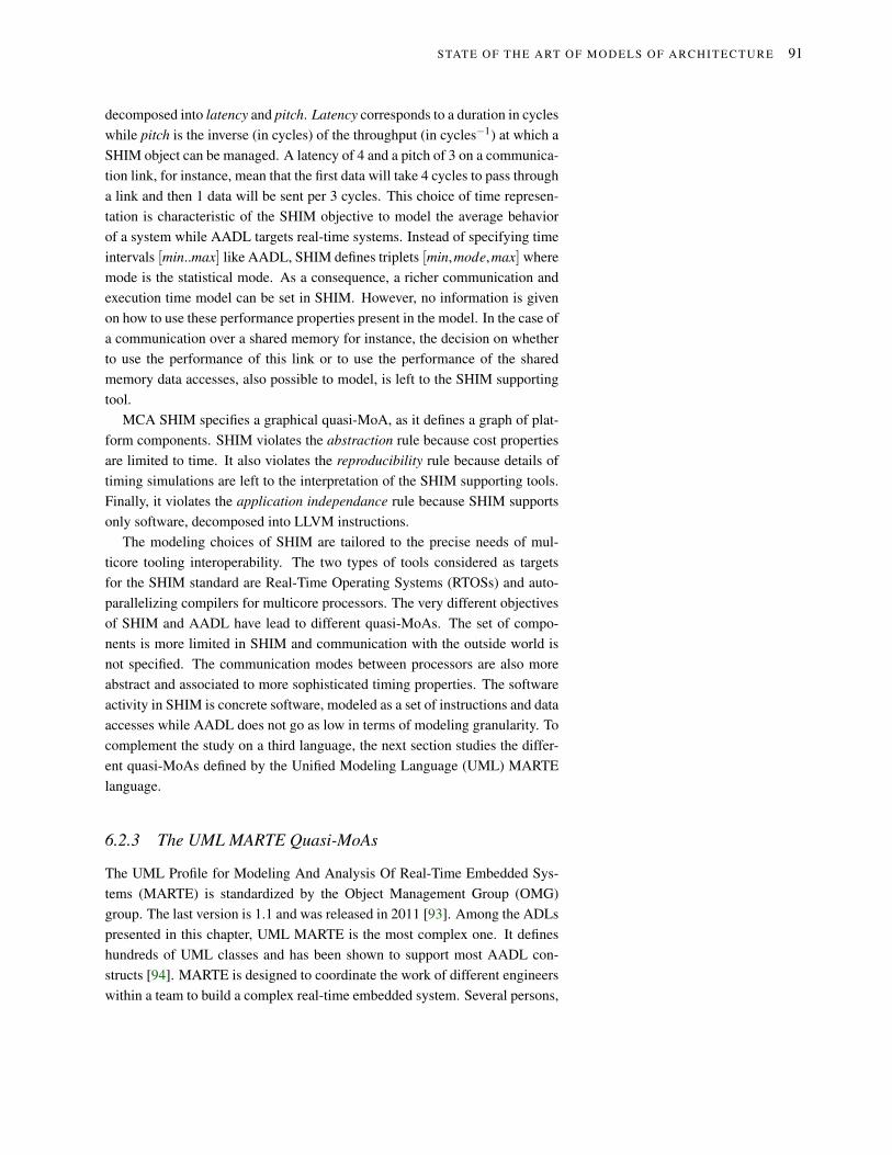
STATE OF THE A RT OF MODELS OF ARC HITEC TURE 91
decomposed into latency and pitch. Latency corresponds to a duration in cycles
while pitch is the inverse (in cycles) of the throughput (in cycles−1) at which a
SHIM object can be managed. A latency of 4 and a pitch of 3 on a communica-
tion link, for instance, mean that the first data will take 4 cycles to pass through
a link and then 1 data will be sent per 3 cycles. This choice of time represen-
tation is characteristic of the SHIM objective to model the average behavior
of a system while AADL targets real-time systems. Instead of specifying time
intervals [min..max] like AADL, SHIM defines triplets [min,mode,max] where
mode is the statistical mode. As a consequence, a richer communication and
execution time model can be set in SHIM. However, no information is given
on how to use these performance properties present in the model. In the case of
a communication over a shared memory for instance, the decision on whether
to use the performance of this link or to use the performance of the shared
memory data accesses, also possible to model, is left to the SHIM supporting
tool.
MCA SHIM specifies a graphical quasi-MoA, as it defines a graph of plat-
form components. SHIM violates the abstraction rule because cost properties
are limited to time. It also violates the reproducibility rule because details of
timing simulations are left to the interpretation of the SHIM supporting tools.
Finally, it violates the application independance rule because SHIM supports
only software, decomposed into LLVM instructions.
The modeling choices of SHIM are tailored to the precise needs of mul-
ticore tooling interoperability. The two types of tools considered as targets
for the SHIM standard are Real-Time Operating Systems (RTOSs) and auto-
parallelizing compilers for multicore processors. The very different objectives
of SHIM and AADL have lead to different quasi-MoAs. The set of compo-
nents is more limited in SHIM and communication with the outside world is
not specified. The communication modes between processors are also more
abstract and associated to more sophisticated timing properties. The software
activity in SHIM is concrete software, modeled as a set of instructions and data
accesses while AADL does not go as low in terms of modeling granularity. To
complement the study on a third language, the next section studies the differ-
ent quasi-MoAs defined by the Unified Modeling Language (UML) MARTE
language.
6.2.3 The UML MARTE Quasi-MoAs
The UML Profile for Modeling And Analysis Of Real-Time Embedded Sys-
tems (MARTE) is standardized by the Object Management Group (OMG)
group. The last version is 1.1 and was released in 2011 [93]. Among the ADLs
presented in this chapter, UML MARTE is the most complex one. It defines
hundreds of UML classes and has been shown to support most AADL con-
structs [94]. MARTE is designed to coordinate the work of different engineers
within a team to build a complex real-time embedded system. Several persons,

92 MODELS , METHODS AND TOOLS FO R BR IDG ING THE DESI GN PRO DUCTI VI TY GAP OF EMBEDDED
SIG NAL PROCESSI NG SY STEMS
expert in UML MARTE, should be able to collaborate in building the system
model, annotate and analyze it, and then build an execution platform from its
model. Like AADL, UML MARTE is focused on hard real-time application
and architecture modeling. MARTE is divided into four packages, themselves
divided into clauses. 3 of these clauses define 4 different quasi-MoAs. These
quasi-MoAs are named QMoAiMART E | i ∈ {1,2,3,4} in this chapter and are
located in the structure of UML MARTE clauses illustrated by the following
list:
• The MARTE Foundations package includes:
– the Core Elements clause that gathers constructs for inheritance and com-
position of abstract objects, as well as their invocation and communica-
tion.
– the Non-Functional Property (NFP) clause that describes ways to spec-
ify non-functional constraints or values (Section 5.2.2), with a concrete
type.
– the Time clause, specific to the time NFP.
– the Generic Resource Modeling (GRM) clause that offers constructs to
model, at a high level of abstraction, both software and hardware ele-
ments. It defines a generic component named Resource, with clocks
and non-functional properties. Resource is the basic element of
UML MARTE models of architecture and application. The quasi-MoA
QMoA1MART E is defined by GRM and based on Resources. It will be
presented in Section 6.2.3.
– the Allocation Modeling clause that relates higher-level Resources to
lower-level Resources. For instance, it is used to allocate Schedulable-
Resources (e.g. threads) to ComputingResources (e.g. cores).
• The MARTE Design Model package includes:
– the Generic Component Model (GCM) clause that defines structured
components, connectors and interaction ports to connect core elements.
– the Software Resource Modeling (SRM) clause that details software re-
sources.
– the Hardware Resource Modeling (HRM) clause that details hardware
resources and defines QMoA2MART E and QMoA3
MART E (Section 6.2.3).
– the High-Level Application Modeling (HLAM) clause that models real-
time services in an OS.
• The MARTE Analysis Model package includes:
– the Generic Quantitative Analysis Modeling (GQAM) clause that spec-
ifies methods to observe system performance during a time interval. It
defines QMoA4MART E .

STATE OF THE A RT OF MODELS OF ARC HITEC TURE 93
– the Schedulability Analysis Modeling (SAM) clause that refers to thread
and process schedulability analysis. It builds over GQAM and adds
scheduling-related properties to QMoA4MART E .
– the Performance Analysis Modeling (PAM) clause that performs proba-
bilistic or deterministic time performance analysis. It also builds over
GQAM.
• MARTE Annexes include Repetitive Structure Modeling (RSM) to compactly
represent component networks, and the Clock Constraint Specification Lan-
guage (CCSL) to relate clocks.
The link between application time and platform time in UML MARTE is
established through clock and event relationships expressed in the CCSL lan-
guage [95]. Time may represent a physical time or a logical time (i.e. a contin-
uous repetition of events). Clocks can have causal relations (an event of clock
A causes an event of clock B) or a temporal relations with type precedence,
coincidence, and exclusion. Such a precise representation of time makes UML
MARTE capable of modeling both asynchronous and synchronous distributed
systems [96]. UML MARTE is capable, for instance, of modeling any kind of
processor with multiple cores and independent frequency scaling on each core.
The UML MARTE resource composition mechanisms give the designer
more freedom than AADL by dividing his system into more than 2 layers.
For instance, execution platform resources can be allocated to operating sys-
tem resources, themselves allocated to application resources while AADL
offers only a hardware/software separation. Multiple allocations to a sin-
gle resource are either time multiplexed (timeScheduling) or distributed in
space (spatialDistribution). Next sections explain the 4 quasi-MoAs defined
by UML MARTE.
The UML MARTE Quasi-MoAs 1 and 4 The UML MARTE GRM clause
specifies the QMoA1MART E quasi-MoA. It corresponds to a graph Λ= 〈M,L, t, p〉
where M is a set of Resources, L is a set of UML Connectors between these
resources, t associates types to Resources and p gives sets of properties to
Resources.
«Processing Resource»
specializes
«Computing Resource» «Communication Media» «Device Resource»
«Storage Resource» «Synchronization Resource»«Timing Resource»
«Concurrency Resource»Figure 6.5: Elements of the quasi-MoA
define in UML MARTE Generic Resource
Modeling (GRM).
7 types of resources are defined in GRM. Some inconsistencies between re-
source relations make the standard ambiguous on resource types. As an exam-
ple, CommunicationMedia specializes CommunicationResource on standard
p.96 [93] while CommunicationMedia specializes ProcessingResource on
standard p.99. SynchResource disappears after definition and is possibly

94 MODELS , METHODS AND TOOLS FO R BR IDG ING THE DESI GN PRO DUCTI VI TY GAP OF EMBEDDED
SIG NAL PROCESSI NG SY STEMS
equivalent to the later SwSynchronizationResource. Considering the most
detailed descriptions as reference, types of resources (illustrated in Figure 6.5)
are:
• a Processing Resource, associated to an abstract speed Factor property
that can help the designer compare different Processing Resources. It
has 3 subtypes: Computing Resource models a real or virtual PE storing
and executing program code. It has no property. Device Resource com-
municates with the system environment, equivalently to an AADL device.
It also has no property. Communication Media can represent a bus or a
higher-level protocol over an interconnect. It has several properties: a mode
among simplex, half-duplex, or full-duplex specifies whether the media is
directed or not and the time multiplexing method for data. Communication
Media transfers one data of elementSize bits per clock cycle. A packet time
represents the time to transfer a set of elements. A block time represents
the time before the media can transfer other packets. A data rate is also
specified.
• a Timing Resource representing a clock or a timer, fixing a clock rate.
• a Storage Resource representing memory, associated with a unit size and
number of units. Memory read and write occur in 1 clock cycle.
• a Concurrency Resource representing several concurrent flows of execu-
tion. It is a generalization of SchedulableResources that model logical
concurrency in threads and processes.
The communication time model of QMoA1MART E , set by the Communication
Media, is the affine model illustrated in Figure 6.4. Precise time properties are
set but the way to correctly compute a timing at system-level from the set of
resource timings is not explicitely elucidated.
QMoA1MART E can be used for more than just time modeling. ResourceUsage
is a way to associate physical properties to the usage of a resource. When
events occur, amounts of physical resources can be specified as “consumed”.
A resource consumption can be associated to the following types of NFPs val-
ues: energy in Joules, message size in bits, allocated memory in bytes, used
memory in bytes (representing temporary allocation), and power peak in Watts.
The Generic Quantitative Analysis Modeling (GQAM) package defines an-
other quasi-MoA (QMoA4MART E ) for performing the following set of analysis:
counting the repetitions of an event, determining the probability of an execu-
tion, determining CPU requirements, determining execution latency, and de-
termining throughput (time interval between two occurrences). New resources
named GaExecHost (ExecutionHost) and GaCommHost (CommunicationHost)
are added to the ones of QMoA1MART E and specialize the ProcessingResource
for time performance and schedulability analysis, as well as for the analysis of
other NFPs. QMoA4MART E is thus close to QMoA1
MART E in terms of resource

STATE OF THE A RT OF MODELS OF ARC HITEC TURE 95
semantics but additional properties complement the quasi-MoA. In terms of
MoAs, QMoA1MART E and QMoA4
MART E have the same properties and none of
them clearly states how to use their properties.
The UML MARTE Quasi-MoAs 2 and 3 The UML MARTE Hardware Re-
source Modeling (HRM) defines two other, more complex quasi-MoAs than
the previously presented ones: QMoA2MART E (logical view) and QMoA3
MART E
(physical view).
An introduction of the related software model is necessary before present-
ing hardware components because the HRM is very linked to the SRM soft-
ware representation. In terms of software, the UML MARTE standard con-
stantly refers to threads as the basic instance, modeled with a swSchedulable-
Resource. The swSchedulableResources are thus considered to be man-
aged by an RTOS and, like AADL, UML MARTE builds on industrial best
practices of using preemptive threads to model concurrent applications. In or-
der to communicate, a swSchedulableResource references specifically de-
fined software communication and synchronization resources.
The HW_Logical subclause of HRM refers to 5 subpackages: HW_Computing,
HW_Communication, HW_Storage, HW_Device, and HW_Timing. It composes
a complex quasi-MoA referred to as QMoA2MART E in this chapter. For brevity
and clarity, we will not enter the details of this quasi-MoA but give some in-
formation on its semantics.
The UML MARTE QMoA2MART E quasi-MoA is, like AADL, based on a
HW/SW separation of concerns rather than on an application/architecture sep-
aration. In terms of hardware, UML MARTE tends to match very finely the
real characteristics of the physical components. UML MARTE HRM is thus
torn between the desire to match current hardware best practices and the ne-
cessity to abstract away system specificities. A QMoA2MART E processing ele-
ment for instance can be a processor, with an explicit Instruction Set Architec-
ture (ISA), caches, and a Memory Management Unit (MMU), or it can be a
Programmable Logic Device (PLD). In the description of a PLD, properties go
down to the number of available LUTs on the PLD. However, modern PLDs
such as FPGAs are far too heterogeneous to be characterized by a number of
LUTs. Moreover, each FPGA has its own characteristics and in the space do-
main, for instance, FPGAs are not based on a RAM configuration memory, as
fixed in the MARTE standard, but rather on a FLASH configuration memory.
These details show the interest of abstracting an MoA in order to be resilient
to the fast evolution of hardware architectures.
HW_Physical composes the QMoA3MART E quasi-MoA and covers coarser-
grain resources than QMoA2MART E , at the level of a printed circuit board. Prop-
erties of resources include shape, size, position, power consumption, heat dis-
sipation, etc.
Interpreting the technological properties of HRM quasi-MoAs QMoA2MART E
and QMoA3MART E is supposed to be done based on designer’s experience be-

96 MODELS , METHODS AND TOOLS FO R BR IDG ING THE DESI GN PRO DUCTI VI TY GAP OF EMBEDDED
SIG NAL PROCESSI NG SY STEMS
cause the UML MARTE properties mirror the terms used for hardware design.
This is however not sufficient to ensure the reproducibility of a cost computa-
tion.
Conclusions on UML MARTE Quasi-MoAs When considering as a whole
the 4 UML MARTE quasi-MoAs, the standard does not specify how the hun-
dreds of NFP standard resource parameters are to be used during simulation
or verification. The use of these parameters is supposed to be transparent,
as the defined resources and parameters match current best practices. How-
ever, best practices evolve over time and specifying precisely cost compu-
tation mechanisms is the only way to ensure tool interoperability in the lon
run. UML MARTE quasi-MoAs do not respect the abstraction rule of MoAs
because, while cost properties target multiple NFPs, each is considered inde-
pendently without capitalizing on similar behaviors of different NFPs. Finally,
QMoA1MART E and QMoA4
MART E respect the application independance rule, and
even extend it to the construction of more than 2 layers, while QMoA2MART E
and QMoA3MART E rather propose a HW/SW decomposition closer to AADL.
6.2.4 Conclusions on ADL Languages
AADL and UML MARTE are both complete languages for system-level de-
sign that offer rich constructs to model a system. MCA SHIM is a domain-
specific language targeted to a more precise purpose. While the 3 languages
strongly differ, they all specify quasi-MoAs with the objective of modeling the
time behavior of a system, as well as other non-functional properties. None
of these 3 languages fully respects the three rules of MoA’s Definition 4. In
particular, none of them abstracts the studied NFPs to make generic the com-
putation of a model’s cost from the cost of its constituents. Abstraction is how-
ever an important feature of MoAs to avoid redesigning redundant simulation
mechanisms.
To complement this study on MoAs, the next section covers four formal
quasi-MoAs from literature.
6.3 Formal Quasi-MoAs
In this Section, we put the focus on graphical quasi-MoAs that aim at pro-
viding system efficiency evaluations when combined with a model of a DSP
application. The models and their contribution are presented chronologically.
6.3.1 The AAA Methodology Quasi-MoA
In 2003, an architecture model is defined for the Algorithm-Architecture Match-
ing (AAA) Y-chart methodology, implemented in the SynDEx tool [97]. The
AAA architecture model is tailored to the needs of an application model that

STATE OF THE A RT OF MODELS OF ARC HITEC TURE 97
splits processing into tasks called operations arranged in a DAG representing
data dependencies between them.
The AAA architecture model is a graphical quasi-MoA Λ = 〈M,L, t, p〉,
where M is a set of components, L is a set of undirected edges connecting
these components, and t and p respectively give a type and a property to com-
ponents. As illustrated in Figure 6.6, there are three types t ∈ T of compo-
nents, each considered internally as a Finite State Machine (FSM) perform-
ing sequencially application management services : memory, sequencer, and
bus/multiplexer/demultiplexer (B/M/D). For their part, edges only model the
capacity of components to exchange data.
component
operator communicator RAM SAM
RAMP RAMD RAMDP
memory B/M/Dsequencer
B/M/D with arb. B/M/D w/o arb.
specializes
P D DP
arbiter
Figure 6.6: Typology of the basic compo-
nents in the AAA architecture model. Leaf
components are instantiable.
In this model, a memory is a Sequencial Access Memory (SAM) or a Random
Access Memory (RAM). A SAM models a FIFO for message passing between
components. A SAM can be point-to-point or multipoint and support or not
broadcasting. A SAM with broadcasting only pops a data when all readers have
read the data. A RAM may store only data (RAMD), only programs (RAMP)
or both (RAMDP). When several sequencers can write to a memory, it has an
implicit arbiter managing writing conflicts.
A sequencer is of type operator or communicator. An operator is a PE
sequencially executing operations stored in a RAMP or RAMDP. An operation
reads and writes data from/to a RAMD or RAMDP connected to the operator.
A communicator models a DMA with a single channel that executes commu-
nications, i.e. operations that transfer data from a memory M1 to a memory
M2. For the transfer to be possible, the communicator must be connected to
M1 and M2.
A B/M/D models a bus together with its multiplexer and demultiplexer that
implement time division multiplexing of data. As a consequence, a B/M/D
represents a sequential schedule of transfered data. A B/M/D may require an
arbiter, solving write conflicts between multiple sources. In the AAA model,
the arbiter has a maximum bandwidth BPMax that is shared between writers
and readers.
Figure 6.7 shows an example, inspired by [97], of a model conforming the
AAA quasi-MoA. It models the 66AK2L06 processor [75] from Texas Instru-
ments illustrated in Figure 5.4 g). Operators must delegate communication to
communicators that access their data memory. The architecture has hardware
cache coherency on ARM side (L2CC for L2 Cache Control) and software
cache coherency on c66x side (SL2C for Software L2 Coherency). The com-

98 MODELS , METHODS AND TOOLS FO R BR IDG ING THE DESI GN PRO DUCTI VI TY GAP OF EMBEDDED
SIG NAL PROCESSI NG SY STEMS
munication between ARML2 and MSMC memories is difficult to model with
AAA FSM components because it is performed by a NoC with complex topol-
ogy and a set of DMAs so it has been represented as a network of B/M/Ds and
communicators in Figure 6.7.
ARM
Cortex-A15
TI c66xL2DP
SL2C
1024KB
L1PP
32KB MSMCDP
2048KB
L2CC
DMA
DMA
DMA
TI c66xL2DP
SL2C
1024KB
TI c66xL2DP
SL2C
1024KB
TI c66xL2DP
SL2C
1024KB
TeraNet
arbiter
ARM
Cortex-A15
L1DD
32KBL2CC
ARML2DP
1024KB
TeraNet
arbiter
TeraNet
arbiter
...
...
DMA
DMA
DMA
L1DD
32KB
L1PP
32KB
Figure 6.7: Example of an architecture de-
scription with the AAA quasi-MoA.
Properties p on components and edges define the quasi-MoA. An operator
Op has an associated function δOp setting a Worst Case Execution Time (WCET)
duration to each operation δOp(o) ∈ R≥0 where O is the set of all operations in
the application. This property results from the primary objective of the AAA
architecture model being the computation of an application WCET. Each edge
of the graph has a maximum bandwidth B in bits/s. The aim of the AAA
quasi-MoA is to feed a multicore scheduling process where application oper-
ations are mapped to operators and data dependencies are mapped to routes
between operators, made of communicators and busses. Each operator
and communicator being an FSM, the execution of operations and communi-
cations on a given sequencer is totally ordered. The application graph being
a DAG, the critical path of the application is computed and represents the la-
tency of one execution, i.e. the time distance beween the beginning of the first
operation and the end of the last operation. The computation of the latency
from AAA application model and quasi-MoA in [97] is implicit. The behavior
of the arbiter is not specified in the model so actual communication times are
subject to interpretations, especially regarding the time quantum for the update
of bandwidth utilization.
The AAA syntax-free quasi-MoA is mimicking the temporal behavior of
a processing hardware in order to derive WCET information on a system.
Many hardware features can be modeled, such as DMAs; shared memories
and hardware FIFO queues. Each element in the model is sequential, making
a coarse-grain model of an internally parallel component impossible. There is
no cost abstraction but the separation between architecture model and applica-
tion model is respected. The model is specific to dataflow application latency
computation, with some extra features dedicated to memory requirement com-
putation. Some performance figures are subject to interpretation and latency
computation for a couple application/architecture is not specified.
The AAA model contribution is to build a system-level architecture model
that clearly separates architecture concerns from algorithm concerns. Next
section discusses a second quasi-MoA, named CHARMED.

STATE OF THE A RT OF MODELS OF ARC HITEC TURE 99
6.3.2 The CHARMED Quasi-MoA
In 2004, the CHARMED co-synthesis framework [98] is proposed that aims
at optimizing multiple system parameters represented in Pareto fronts. Such
a multi-parameter optimization is essential for DSE activities, as detailed in
[99].
In the CHARMED quasi-MoA Λ = 〈M,L, t, p〉, M is a set of PEs, L is a set
of Communication Resources (CR) connecting these components, and t and
p respectively give a type and a property to PEs and CRs. There is only one
type of component so in this model, t = PE. Like in the AAA architecture
model, PEs are abstract and may represent programmable microprocessors as
well as hardware IPs. The PE vector of properties p is such that p(PE ∈ M) =
[α ,κ , µd , µi,ρidle]T where α denotes the area of the PE, κ denotes the price
of the PE, µd denotes the size of its data memory, µi denotes the instruction
memory size and ρidle denotes the idle power consumption of the PE. Each CR
edge also has a property vector: p(CR ∈ L) = [ρ ,ρidle,θ ]T where ρ denotes
the average power consumption per each unit of data to be transferred, ρidle
denotes idle power consumption and θ denotes the worst case transmission
rate or speed per each unit of data.
This model is close to the concept of MoA as stated by Definition 4. How-
ever, instead of abstracting the computed cost, it defines many costs altogether
in a vector. This approach limits the scope of the approach and CHARMED
metrics do not cover the whole spectrum on NFPs shown in Section 5.2.2.
The CHARMED architecture model is combined with a DAG task graph of a
stream processing application in order to compute costs for different system
solutions. A task in the application graph is characterized by its required in-
struction memory µ , its Worst Case Execution Time WCET and its average
power consumption ℘avg while a DAG edge is associated with a data size δ .
The cost for a system x has 6 dimensions: the area α(x), the price κ(x), the
number of used inter-processor routes ln(x), the memory requirements µ(x),
the power consumption ℘(x) and the latency τ(x). Each metric has an op-
tional maximum value and can be set either as a constraint (all values under
the constraint are equally good) or as an objective to maximize.
Cost computation is not fully detailed in the model. We can deduce from
definitions that PEs are sequential units of processing where tasks are time-
multiplexed and that a task consumes℘avg×WCET energy for each execution.
The power consumption for a task is considered independent of the PE execut-
ing it. The latency is computed after a complete mapping and scheduling of
the application onto the architecture. The price and area of the system are the
sums of PE prices and areas. Memory requirements are computed from data
and instruction information respectively on edges and tasks of the application
graph. Using an evolutionary algorithm, the CHARMED framework produces
a set of potential heterogeneous architectures together with task mappings onto
these architectures.

100 MODELS , METHODS AND TOOLS FO R BR IDG ING THE DESI GN PRODUCTI VI TY GA P OF EMBEDDED
SIG NAL PROCESSI NG SY STEMS
For performing DSE, the CHARMED quasi-MoA has introduced a model
that jointly considers different forms of NFP metrics. The next section presents
a third quasi-MoA named System-Level Architecture Model (S-LAM).
6.3.3 The System-Level Architecture Model (S-LAM) Quasi-MoA
In 2009, the S-LAM model 5 is proposed to be inserted in the PREESM rapid 5 M. Pelcat, J.-F. Nezan, J. Piat, Jerome
Croizer, and S. Aridhi. A system-level ar-
chitecture model for rapid prototyping of het-
erogeneous multicore embedded systems. In
Proceedings of DASIP conference, 2009
prototyping tool. S-LAM is designed to be combined with an application
model based on extensions of the Synchronous Dataflow (SDF) dataflow MoC
and a transformation of a UML MARTE architecture description into S-LAM
has been conducted in 6. 6 Manel Ammar, Mouna Baklouti, Maxime
Pelcat, Karol Desnos, and Mohamed Abid.
Automatic generation of s-lam descriptions
from uml/marte for the dse of massively par-
allel embedded systems. In Software En-
gineering, Artificial Intelligence, Networking
and Parallel/Distributed Computing 2015.
Springer, 2016
S-LAM defines a quasi-MoA Λ = 〈M,L, t, p〉 where M is a set of com-
ponents, L is a set of links connecting them, and t and p respectively give a
type and a property to components. As illustrated in Figure 6.8, there are five
instantiable types of components: operator, parallel node, contention
node, RAM, and DMA.
component link
data link
directed data link undirected data link
control link
RAM DMA
communicationenabler
operatorcommunicationnode
parallel node contention node
refines
Figure 6.8: Typology of the basic compo-
nents in the S-LAM. Leaf components are
instantiable.
Operators represent astract processing elements, capable of executing tasks
(named actors in dataflow models) and of communicating data through links.
Actors’ executions are time-multiplexed over operators, as represented by the
black dot on the graphical view, symbolizing scheduling. There are also data
links and control links. A data link represents the ability to transfer
data between components. Control links specify that an operator can pro-
gram a DMA. Two actors can not be directly connected by a data link. A route
must be built, comprising at least one parallel node or one contention
node. A parallel node Np virtually consists of an infinite number of data
channels with a given speed σ(Np) in Bytes/s. As a consequence, no schedul-
ing is necessary for the data messages sharing a parallel node. A contention
node Nc represents one data channels with speed σ(Nc). Messages flowing
over a contention node need to be scheduled, as depicted by the black dot
in its representation. This internal component parallelism is the main novelty
of S-LAM w.r.t. the AAA model. When transferring a data from operator O1
to operator O2, three scenarios are considered:
1. direct messaging: the sender operator itself sends the message and, as a
consequence, cannot execute code simultaneously. It may have direct ac-
cess to the receiver’s address space or use a messaging component.
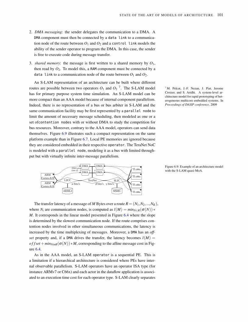
STATE OF THE ART OF MODELS OF ARC HITEC TURE 101
2. DMA messaging: the sender delegates the communication to a DMA. A
DMA component must then be connected by a data link to a communica-
tion node of the route between O1 and O2 and a control link models the
ability of the sender operator to program the DMA. In this case, the sender
is free to execute code during message transfer.
3. shared memory: the message is first written to a shared memory by O1,
then read by O2. To model this, a RAM component must be connected by a
data link to a communication node of the route between O1 and O2.
An S-LAM representation of an architecture can be built where different
routes are possible between two operators O1 and O27. The S-LAM model 7 M. Pelcat, J.-F. Nezan, J. Piat, Jerome
Croizer, and S. Aridhi. A system-level ar-
chitecture model for rapid prototyping of het-
erogeneous multicore embedded systems. In
Proceedings of DASIP conference, 2009
has for primary purpose system time simulation. An S-LAM model can be
more compact than an AAA model because of internal component parallelism.
Indeed, there is no representation of a bus or bus arbiter in S-LAM and the
same communication facility may be first represented by a parallel node to
limit the amount of necessary message scheduling, then modeled as one or a
set ofcontention nodes with or without DMA to study the competition for
bus resources. Moreover, contrary to the AAA model, operators can send data
themselves. Figure 6.9 illustrates such a compact representation on the same
platform example than in Figure 6.7. Local PE memories are ignored because
they are considered embedded in their respective operator. The TeraNet NoC
is modeled with a parallel node, modeling it as a bus with limited through-
put but with virtually infinite inter-message parallelism.
L2CC
ARMCortex-A15
ARMCortex-A15
TeraNet
ARML2
SL2C
MSMC
DMA
DMA
DMA
DMATI c66x
TI c66x
TI c66x
TI c66x
α bits/s β bits/s γ bits/s
DMA progtime (s)
Figure 6.9: Example of an architecture model
with the S-LAM quasi-MoA.
The transfer latency of a message of M Bytes over a route R= (N1,N2, ...,NK),
where Ni are communication nodes, is computed as l(M) = minN∈R(σ(N)) ∗
M. It corresponds in the linear model presented in Figure 6.4 where the slope
is determined by the slowest communication node. If the route comprises con-
tention nodes involved in other simultaneous communications, the latency is
increased by the time multiplexing of messages. Moreover, a DMA has an off-
set property and, if a DMA drives the transfer, the latency becomes l(M) =
o f f set +minNinR(σ(N))∗M, corresponding to the affine message cost in Fig-
ure 6.4.
As in the AAA model, an S-LAM operator is a sequential PE. This is
a limitation if a hierarchical architecture is considered where PEs have inter-
nal observable parallelism. S-LAM operators have an operator ISA type (for
instance ARMv7 or C66x) and each actor in the dataflow application is associ-
ated to an execution time cost for each operator type. S-LAM clearly separates

102 MODELS , METHODS AND TOOLS FO R BR IDG ING THE DESI GN PRODUCTI VI TY GA P OF EMBEDDED
SIG NAL PROCESSI NG SY STEMS
algorithm from architecture but it does not specify cost computation and does
not abstract computation cost.
S-LAM has introduced a compact quasi-MoA to be used for DSP applica-
tions. The next section presents one last quasi-MoA from literature.
6.3.4 The MAPS Quasi-MoA
In 2012, a quasi-MoA is proposed in [102] for programming heterogeneous
MPSoCs in the MAPS compiler environment. It combines the multi-modality
of CHARMED with a sophisticated representation of communication costs.
The quasi-MoA serves as a theoretical background for mapping multiple con-
current transformational applications over a single MPSoC. It is combined
with KPN application representations [103] and is limited to the support of
software applications.
The MAPS quasi-MoA is a graph Λ = 〈M,L, t, p〉 where M is a set of PEs,
L is a set of named edges called Communication Primitives (CPs) connecting
them, and t and p respectively give a type and a property to components. Each
PE has properties p(PE ∈ M) = (CMPT ,XPT ,V PT ) where CMPT is a set of
functions associating NFP costs to PEs. An example of NFP is ζ PT that as-
sociates to a task Ti in the application an execution time ζ PT (Ti). XPT is a
set of PE attributes such as context switch time of the OS or some resource
limitations, and V PT is a set of variables, set late after application mapping
decisions, such as the processor scheduling policy. A CP models a software
Application Programming Interface (API) that is used to communicate among
tasks in the KPN application. A CP has its own set of cost model functions
CMCP associating costs of different natures to communication volumes. A
function ζCP ∈CMCP is defined. It associates a communication time ζCP(N)
to a message of N bytes. Function ζCP is a stair function modeling the mes-
sage overhead and performance bursts frequently observed when transferring
data for instance with a DMA and packetization. This function, displayed in
Figure 6.4, is expressed as:
ζCP : N 7→=
{
o f f set i f N < start
o f f set + scale_height ×⌈(N − start + 1)/scale_width⌉ otherwise,
(6.1)
where start, o f f set, scale_height and scale_width are 4 CP parameters. The
primary concern of the MAPS quasi-MoA is thus time. No information is
given on whether the sender or the receiver PE can compute a task in parallel to
communication. A CP also refers to a set of Communication Resources (CRs),
i.e. a model of a hardware module used to implement the communication.
A CRs has two attributes: the number of logical channels and the amount of
available memory in the module. For example, a CR may model a shared
memory, a local memory, or a hardware communication queue.
This quasi-MoA does not specify any cost computation procedure from the
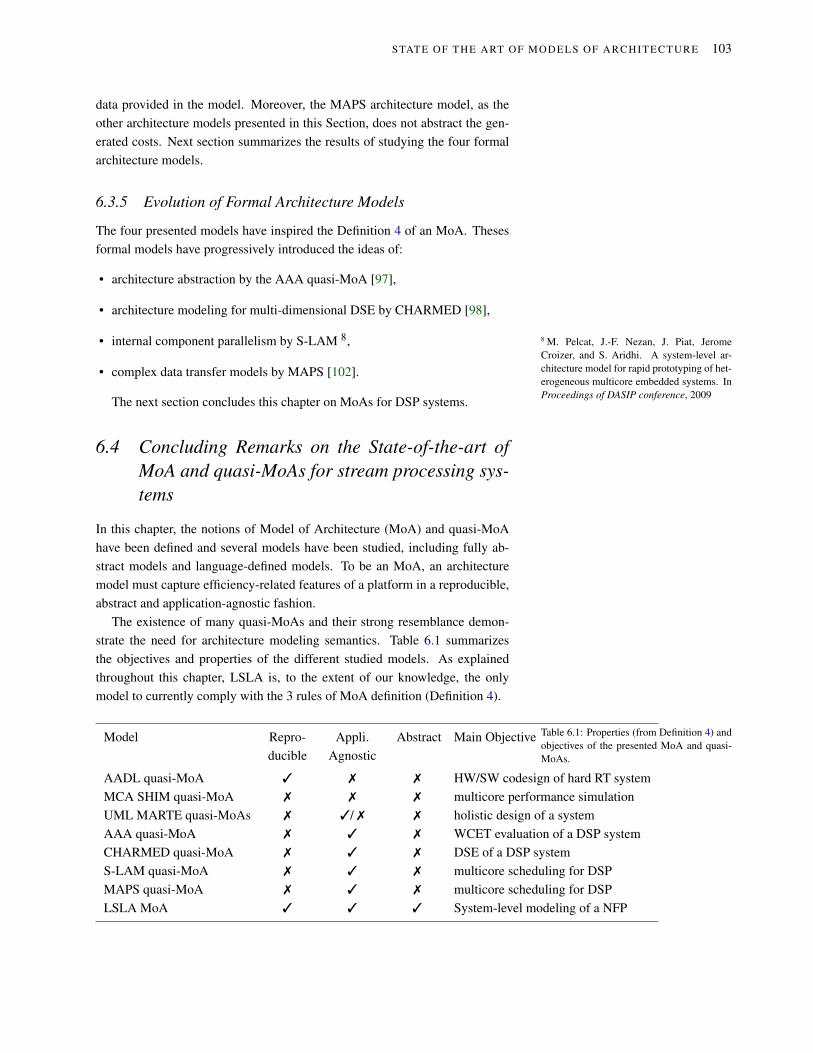
STATE OF THE ART OF MODELS OF ARC HITEC TURE 103
data provided in the model. Moreover, the MAPS architecture model, as the
other architecture models presented in this Section, does not abstract the gen-
erated costs. Next section summarizes the results of studying the four formal
architecture models.
6.3.5 Evolution of Formal Architecture Models
The four presented models have inspired the Definition 4 of an MoA. Theses
formal models have progressively introduced the ideas of:
• architecture abstraction by the AAA quasi-MoA [97],
• architecture modeling for multi-dimensional DSE by CHARMED [98],
• internal component parallelism by S-LAM 8, 8 M. Pelcat, J.-F. Nezan, J. Piat, Jerome
Croizer, and S. Aridhi. A system-level ar-
chitecture model for rapid prototyping of het-
erogeneous multicore embedded systems. In
Proceedings of DASIP conference, 2009
• complex data transfer models by MAPS [102].
The next section concludes this chapter on MoAs for DSP systems.
6.4 Concluding Remarks on the State-of-the-art of
MoA and quasi-MoAs for stream processing sys-
tems
In this chapter, the notions of Model of Architecture (MoA) and quasi-MoA
have been defined and several models have been studied, including fully ab-
stract models and language-defined models. To be an MoA, an architecture
model must capture efficiency-related features of a platform in a reproducible,
abstract and application-agnostic fashion.
The existence of many quasi-MoAs and their strong resemblance demon-
strate the need for architecture modeling semantics. Table 6.1 summarizes
the objectives and properties of the different studied models. As explained
throughout this chapter, LSLA is, to the extent of our knowledge, the only
model to currently comply with the 3 rules of MoA definition (Definition 4).
Model Repro-
ducible
Appli.
Agnostic
Abstract Main Objective
AADL quasi-MoA ✓ ✗ ✗ HW/SW codesign of hard RT system
MCA SHIM quasi-MoA ✗ ✗ ✗ multicore performance simulation
UML MARTE quasi-MoAs ✗ ✓/ ✗ ✗ holistic design of a system
AAA quasi-MoA ✗ ✓ ✗ WCET evaluation of a DSP system
CHARMED quasi-MoA ✗ ✓ ✗ DSE of a DSP system
S-LAM quasi-MoA ✗ ✓ ✗ multicore scheduling for DSP
MAPS quasi-MoA ✗ ✓ ✗ multicore scheduling for DSP
LSLA MoA ✓ ✓ ✓ System-level modeling of a NFP
Table 6.1: Properties (from Definition 4) and
objectives of the presented MoA and quasi-
MoAs.

104 MODELS , METHODS AND TOOLS FO R BR IDG ING THE DESI GN PRODUCTI VI TY GA P OF EMBEDDED
SIG NAL PROCESSI NG SY STEMS
LSLA is one example of an MoA but many types of MoAs are imaginable,
focusing on different modalities of application activity such as concurrency
or spatial data locality. A parallel with MoCs on the application side of the Y-
chart motivates for the creation of new MoAs. MoCs have the ability to greatly
simplify the system-level view of a design, and in particular of a DSP design.
For example, MoCs based on Dataflow Process Networks (DPNs) are able to
simplify the problem of system verification by defining globally asynchronous
systems that synchronize only when needed, i.e. when data moves from one
location to another. DPN MoCs are naturally suited to modeling DSP applica-
tions that react upon arrival of data by producing data. MoAs to be combined
with DPN MoCs do not necessarily require the description of complex rela-
tions between data clocks. They may require only to assess the efficiency of
“black box” PEs, as well as the efficiency of transferring, either with shared
memory or with message passing, some data between PEs. This opportunity is
exploited in the semantics of the 4 formal languages presented in Section 6.3
and can be put in contrast with the UML MARTE standard that, in order to sup-
port all types of transformational and reactive applications, specifies a generic
clock relation language named CCSL [95].
The 3 properties of an MoA open new opportunities for system design.
While abstraction makes MoAs adaptable to different types of NFPs, cost com-
putation reproducibility can be the basis for advanced tool compatility. Inde-
pendance from application concerns is moreover a great enabler for Design
Space Exploration methods.
Architecture models are also being designed in other domains than Digital
Signal Processing. As an example in the HPC domain, the Open MPI Portable
Hardware Locality (hwloc) [104] models processing, memory and communi-
cation resources of a platform with the aim of improving the efficiency of HPC
applications by tailoring thread locality to communication capabilities. Sim-
ilarly to most of the modeling features described in this chapter, the hwloc
features have been chosen to tackle precise and medium-term objectives. The
convergence of all these models into a few generic MoAs covering different
aspects of design automation is a necessary step to manage the complexity of
future large scale systems.
The next chapter complements our study by illustrating the use of an MoA
on a practical case study.

7
Models of Architecture in Practice
Figure 7.1: The Odroid XU3 board used
for measuring execution energy consumption
and learning a LSLA MoA.
7.1 Chapter Abstract
The MoA named Linear System-Level Architecture Model (LSLA) has been
introduced in Section 5.3.2. As an MoA, it abstracts the internal organisa-
tion of a computing platform. This MoA has also been demonstrated in the
Section 5.3.2 to compute an abstract NFP cost when combined with a SDF
modeled application. Its linear nature comes from the fact that it computes
a NFP cost as a linear combination of individual costs due to an application
activity.
In this chapter, LSLA is further studied in collaboration with SDF. The
Chapter demonstrates the capacity of a simple LSLA MoA to model in prac-
tice the energy consumption of a complex MPSoC. The parameters of the LSLA
model are learnt from physical measurements of the platform energy consump-
tion by linear regression. The additive nature of energy consumption is used to
abstract away many of the hardware and software features and still efficiently
predict energy.
The generated model is shown to represent the hardware behavior with a
fidelity of 86% while the model remains simple and inexpensive. Such result is
a great incentive to progress further in MoA semantics formulation and MoA-
based system design.
7.2 Learning an LSLA Model from Platform Mea-
surements
This section first introduces a method to learn the parameters of a LSLA model
from hardware measurements of the MoA-modeled cost. The method being
based on algebra, the next section presents an algebraic representation of an
LSLA model. This study has been made public in a research report1.
1 Maxime Pelcat, Alexandre Mercat, Karol
Desnos, Luca Maggiani, Yanzhou Liu, Julien
Heulot, Jean-François Nezan, Wassim Hami-
douche, Daniel Menard, and Shuvra S
Bhattacharyya. Models of Architecture:
Application to ESL Model-Based Energy
Consumption Estimation. Research re-
port, IETR/INSA Rennes ; Scuola Superiore
Sant’Anna, Pisa ; Institut Pascal ; University
of Maryland, College Park ; Tampere Univer-
sity of Technology, Tampere, 2017

106 MODELS , METHODS AND TOOLS FO R BR IDG ING THE DESI GN PRODUCTI VI TY GA P OF EMBEDDED
SIG NAL PROCESSI NG SY STEMS
7.2.1 Algebraic Expression of costs in an LSLA Model
Let us consider an LSLA model (Section 5.3.2) with fixed topology, i.e. the
sets P, C and L of respectively PEs, CNs and Links are fixed. The param-
eters αn and βn are initially unknown and will be learnt from measurements
of the modeled non-functional property on the platform (e.g. energy). The
Lagrangian coefficient λ is fixed to 1. The parameters of an LSLA MoA are
gathered in a vector m of size 2η such that:
m = (αn,∀n ∈ P∪C;βn,∀n ∈ P∪C). (7.1)
The size of 2η is due to the concatenation of token- and quanta-related
parameters. An arbitrary order is thus chosen for PEs and CNs and the per-
quantum costs αn and per-token costs βn are concatenated in a unique vector.
7.2.2 Applying Parameter Estimation to LSLA Model Inference
Parameter estimation [105] consists of solving an inverse problem to learn the
parameters of a model from real-life measurements. In the case of LSLA, the
relationship between activity and cost is assumed to be linear and the inverse
problem is solved by a linear regression. A series of measured cost d can be
ideally expressed as the result of the following forward problem:
d = Gm+ ε , (7.2)
where d = (d1, ...,dM)T is a set of M cost samples (e.g. energy samples), m is
the vector of 2η costs defined in Equation 7.1, ε is the measurements noise
resulting in the error vector ε = (ε1, ...,εm), and each line Gk ∈ G corresponds
to an activity vector containing the number of quanta and tokens mapped to the
corresponding PEs or CNs for a sample dk. Gk can be decomposed into:
Gk = (∑size(τ),∀τ ∈ Mk(n1);
∑size(τ),∀τ ∈ Mk(n2); ...;∑size(τ),∀τ ∈ Mk(nη );
card(Mk(n1));card(Mk(n2)); ...;card(Mk(nη )))
(7.3)
where Mk : P ∪C → TP ∪ TC is the mapping function for experiment k that
associates to each PE or CN the set of tokens executed by this component.
card refers to the cardinality of the considered set, i.e. the number of tokens
while the sum of sizes return the number of quanta.
In order to obtain reliable parameter values, the system is overdetermined
by performing more measurements than there are parameters in the model,
i.e. M >> 2η . Furthermore, the error vector ε is assumed as random vari-
able with zero mean µε and constant standard deviation σε among samples.
From the forward problem in Equation 7.2, we can derive the Ordinary Least
Square (OLS) solution to the inverse problem [105]:
mL2 = (GTG)−1
GT
d. (7.4)

MODELS O F ARCH ITECTU RE IN PRACTI CE 107
This equation performs the training of the model. mL2 is thus a set of pa-
rameters αn and βn, deduced from measurements d, that can be entered in the
LSLA model. For a new system activity G′, cost evaluation is computed with:
dLSLA = G
′mL2. (7.5)
This equation performs the prediction of the cost based on the LSLA model
and on the application activity. The residual error of the prediction can be
evaluated as follows:
εm = dLSLAm −dm m = 1, ...,M (7.6)
where the error term is expressed as the deviation between measures and the
trained model. Such residuals represent the measures’ variability that is not
considered in the regression model (e.g., correlated side-effect among mea-
sures) [106]. In section 7.3.4, the impact of the error term ε on the trained
model is empirically evaluated. In the next section, parameter inference is put
into practice for predicting the energy consumption of an MPSoC.
7.3 Experimental Evaluation with LSLA of an MP-
SoC Energy Consumption
7.3.1 Objectives and Modeled Hardware Architecture
We intend to model with LSLA the dynamic energy consumption when exe-
cuting an application, modeled with SDF, on an MPSoC running at full speed
where the number of cores reserved for the application is tuned. The moti-
vation for this study lies in the hypothesis that dynamic energy consumption
depends additively on application activity.
The modeled architecture is an Exynos 5422 processor from Samsung. This
processor is integrated in an Odroid-XU3 platform that offers real-time power
consumption measurements of the cores and memory. The Exynos 5422 pro-
cessor embeds 8 ARM cores in a big.LITTLE configuration. Four of the cores
are of type Cortex-A7 and form an A7 cluster sharing a clock with frequency
up to 1.4GHz. The four remaining cores are of type Cortex-A15 and form an
A15 cluster with frequency up to 2GHz. An external Dynamic Random Access
Memory (DRAM) of 2GBytes is connected as a Package on Package (PoP). A
Linux Ubuntu Symmetric Multiprocessing (SMP) operating system is running
on the platform. Four Texas Instruments INA231 power sensors measure the
instantaneous power of the A7 cluster, the A15 cluster, the Graphics Process-
ing Unit (GPU) and the external DRAM memory. The energy consumed by
the GPU is left out of the scope of the chapter but its modeling with an MoA
constitutes a promising extension. Power values are read from an I2C driver. A
lightweight script runs in parallel to the measured program, forces the proces-
sor to run at full speed and reports current and voltage at 10Hz during program

108 MODELS , METHODS AND TOOLS FO R BR IDG ING THE DESI GN PRODUCTI VI TY GA P OF EMBEDDED
SIG NAL PROCESSI NG SY STEMS
execution. This data is exported into files to be processed offline. In our experi-
ments, the power measurements from the A7 and A15 clusters and the memory
are summed up and used as the energy consumption vector d.
7.3.2 Choosing the lsla topology
We consider a fixed target platform from which a model is learnt. While the
parameters set on PEs and CNs are learnt, their number and topology are cho-
sen, based on assumptions and on prior knowledge of the real hardware fea-
tures. This type of model is qualified as a “hybrid combination of mechanistic
and empirical modeling” in [99]. Mechanistic choices are made “from a ba-
sic understanding of the mechanics of the modeled system” while empirical
modeling corresponds to the set of trained parameters. A method is introduced
hereunder to perform the mechanistic choices. It is assumed that the hardware
being characterized preexists the study. The method is decomposed into:
1. the number of coarse-grain PEs to consider in the study (cores, coproces-
sors, GPUs...) is determined. One PE is instantiated in the model per con-
sidered physical PE on the platform,
2. the different communication hardware features on the platform for inter-
core communication are located (including shared bus, DMA, shared mem-
ory, hardware cache coherency management, etc.). If several PEs share the
same communication hardware feature, one CN is allocated on the model,
connected to all the cores sharing this feature,
3. if communication hardware features, already modeled by CNs, are them-
selves communicating through "higher-level" hardware communication, a
new CN is created and connected to their corresponding CNs,
4. step 3 is repeated until the MoA forms a connected component.
Applying this method to the experimental setup, the 8 PEs corresponding
to the 8 cores of the Exynos 5422 processor are first instantiated. Then, each
cluster being connected by a shared memory with hardware cache coherency,
A7 and A15 clusters are each associated to a CN connecting the 4 cores of the
CN. Finally, The ARM ACE (AXI Coherency Extension) higher-level cache
coherency protocol, connecting the two clusters, is associated to a CN. The
resulting model is shown at the bottom of Figure 7.2.
Once this mechanistic model creation step has been performed, the model
may be simplified to reduce its number of parameters. First, two connected
CNs may be connected if 1- the number of tokens crossing each CN is forecast
or measured to be equivalent, or 2- one of the 2 CNs is forecast or measured
to strongly dominate the other in terms of generated cost. Moreover, equiv-
alently performing PEs can be merged to simplify the model. Such a model
simplification will be experimented in Section 7.3.4.

MODELS O F ARCH ITECTU RE IN PRACTI CE 109
7.3.3 Experimental Setup
PREESMmulticorescheduler
A7A15A15
A15
A7
A7 A7 A15
Application(PiSDF)
PREESMSDF
generator
fixingapplicationparameters
(configuration)
Texas Instruments
INA 231 power monitor
architecturemodel
applicationSDF model G
CC C
ompile
r
C code of the SDF actors
PREESMcode gen.
measuring energyfor E application executions
Linux Multicore OS
3) Code Generation
5) LearningModelParameters
LSLA architecture
applicationactivity
measuredenergy
A15CN PE6
PE5
PE8
PE7
PE2A7CN
PE1αPE1.s+βPE1
PE3
PE4
ICC
λ=1
αPE2.s+βPE2
αPE3.s+βPE3
αPE4.s+βPE4
αPE5.s+βPE5
αPE6.s+βPE6
αPE7.s+βPE7
αPE8.s+βPE8
αA7CN.s+βA7CN
αICC.s+βICC
αA15CN.s+βA15CN
1) Executableapplicationspecification
2) Static Mapping and Scheduling
4) ExecutingApplication
6) Energy prediction from LSLA
Figure 7.2: Experimental setup for inferring
the LSLA execution energy model of a Sam-
sung Exynos 5422 MPSoC.Software Tools Figure 7.2 summarizes the experimental setup used to train
and test the LSLA MoA of an Exynos 5422 processor from energy measure-
ments. The PREESM dataflow framework 2 is used to generate code for dif- 2 M. Pelcat, K. Desnos, J. Heulot, C. Guy,
J.-F. Nezan, and S. Aridhi. PREESM: A
dataflow-based rapid prototyping framework
for simplifying multicore dsp programming.
In Proceedings of the EDERC Conference,
Sept 2014
ferent SDF configurations of a stereo matching application from a PiSDF exe-
cutable specification (Section 2.3.2. The motivation for using a PiSDF descrip-
tion is that, by fixing various values for application parameters, different func-
tional SDF applications are obtained. Once the parameters of the application
are fixed, PREESM generates an executable SDF graph that feeds a multicore
mapper and scheduler. Mapping and scheduling are statically and automati-
cally computed, based on the list scheduling algorithm from [35]. PREESM
then generates a self-timed multicore code for the application that runs on the
target platform. The internal code of the actors is manually written in C code.
PREESM manages the inter-core communication and allocates the application
buffers statically in the .bss segment of the executable. PREESM generates
one thread per target core and forces the thread to the corresponding core via
affinities.
Communication between actors occurs through shared memory with cache
coherency between different threads. Semaphores are instantiated to synchro-
nize memory accesses. The whole procedure of mapping, scheduling and gen-
erating code with PREESM is either manually launched or scripted. For the
current experiment, scripts have been developed to automate large numbers of
code generations, compilations, application executions and energy measure-
ments. An application activity exporter has also been added to PREESM that
computes the activity for each core, from which αn and βn LSLA parameters
are learnt. Finally, once its parameters have been learnt, the LSLA model of
the platform can be used, together with application activity information, to

110 MODELS , METHODS AND TOOLS FO R BR IDG ING THE DESI GN PRODUCTI VI TY GA P OF EMBEDDED
SIG NAL PROCESSI NG SY STEMS
predict the energy consumption of the platform.
Benchmarked Application The stereo matching algorithm from 3, shown in 3 A. Mercat, J.-F. Nezan, D. Menard, and
J. Zhang. Implementation of a stereo match-
ing algorithm onto a manycore embedded
system. In Proceedings of the ISCAS con-
ference. IEEE, 2014
its SDF form in Figure 7.3, is used for the study. From a pair of views of the
same scene, the stereo matching application computes a disparity map, corre-
sponding to the depth of the scene for each pixel. The disparity corresponds
to the distance in pixels between the representations of the same object in both
views. Parameters can be customized such as the size of the input images,
the number of tested disparities and the number of refinement iterations in the
algorithm. These parameters allow for various configurations and application
activities to be created. The tested configurations for this study are summa-
rized in Table 7.1. The size of the obtained SDF graph is stated, as well as its
maximum speedup in latency if executed on a homogeneous architecture with
an infinite number of Cortex-A7 cores and costless communication.
Configuration ID 1 2 3 4 5 6
input image size 450×375 90×75 270×225
# disparities 30 2 15 60 60 60
# iterations 4 2 3 4 4 4
# of actors 177 67 134 297 317 317
total # of FIFOs 560 102 323 1040 1050 1050
max. speedup 6× 2.5× 4.7× 6.6× 6.5× 6.6×
Table 7.1: Configurations of the stereo
matching application employed to assess the
energy modelling.
The stereo matching application is open source and available at 4. Below 4 K. Desnos and J. Zhang. PREESM
project - stereo matching, 2017.
svn://svn.code.sf.net/p/preesm/code/trunk/tests/stereoeach actor in the SDF graph of Figure 7.3 is a repetition factor indicating the
number of actor executions during an iteration of the graph. This number
is deduced from the data production and consumption rates of actors. Two
parameters are shown in the graph: NbDisparities represents the number of
distinct values that can be found in the output disparity map, and NbOffsets
is a parameter influencing the size of the pixel area considered for the pixel
weight and aggregation calculus of the algorithm. NbIterations affects the
computational load of actors.
The SDF graph contains 12 distinct actors: ReadRGB reads from a file the
RGB data of an image, BrdX is a broadcast actor. It duplicates on its out-
put ports the data token consumed on its input port. It generates only pointer
manipulations in the code. GetLeft gets the RGB left view of the stereo pair.
RGB2Gray converts an RGB image into grayscale. Census produces an 8-bit
signature for each pixel, obtained by comparing the pixel to its 8 neighbors: if
the value of the neighbor is greater than the value of the pixel, the signature bit
is set to 1, and otherwise to 0. CostConstruction is executed once per potential
disparity level. By combining the two images and their census signatures, it
produces for each pixel the cost of matching this pixel from the first image
with the corresponding pixel in the second image shifted by a disparity level.
ComputeWeights produces 3 weights for each pixel, using characteristics of

MODELS O F ARCH ITECTU RE IN PRACTI CE 111
neighboring pixels. AggregateCosts computes the matching cost of each pixel
for a given disparity. Computations are based on an iterative method that is
executed NbOffsets times. DisparitySelect produces a disparity map by com-
puting the disparity of the input cost map from the lowest matching cost for
each pixel. RoundBuffer forwards the last disparity map consumed on its input
port to its output port. MedianFilter applies a 3×3 pixels median filter to the
input disparity map to smooth the results. The filter is data parallel and 15
occurrences of the actor are fired to process 15 slices in the image. Finally,
Display writes the depth map in a file.
ReadRGB
3
3
3
2*3
2*3 2
2
1
1
2
12*3
2*3
3rgb
3*2*NbOffsets
3*2*NbOffsets
3*2*NbOffsets*NbDisparities
3
3
3*2*NbOffsets
x1
NbDisparities
1 1 1
11
1
111
1
2*NbDisparities
2
2
2*NbDisparitiesBrd0i o0
o1
rgb
RGB2Graygray
GetLeftrgb rgbLeft
cen
cost
Brd1i o0
o1
Censusgray cen
Brd2i o
Brd3i o weight
Brd4i o
cost
weights
aggregate aggregate
feed
result
back
i o result filtered filtered
gray
CostConstruction
DisparitySelectAggregateCosts
rgbLeft
DisplayMedianFilterRoundBuffer
ComputeWeights
x1
x2 x1
x1x1 x2*NbOffsets
x1xNbDisparitiesxNbDisparities
x1x15
xNbDisparitiesx1x2
x1x2
Figure 7.3: Illustration of the stereo match-
ing application graph. The number of dupli-
cations of each actor is specified. All rates
are implicitly multiplied by the picture size.
The SDF description of the algorithm provides a high degree of parallelism
since it is possible to execute in parallel the repetitions of the three most com-
putationally intensive actors: CostConstruction, AggregateCosts, and Com-
puteWeights.
The generated application code is compiled by GCC with −O3 optimiza-
tion. For each configuration, 255 different PE mappings are tested by enabling
different subsets of the platform cores. PREESM schedules the application on
the subsets with the objective of minimizing application latency.
Energy Measurements Only the dynamic energy consumption is considered
in this experiment. All the eight cores are activated and their frequency is fixed
at their maximum. Thus, the static power, measured at 2.4362W in the given
conditions, is subtracted from power samples. d in Equation 7.2 is a vector of
energy samples expressed in Joules. The energy of an application execution is
measured by integrating the instantaneous power consumed by the A7 cluster,
the A15 cluster and the memory during application execution time.
The unit being measured and analyzed is one execution of the application,
from the beginning of the retrieval of 2 images to the end of the production of a
depth map. By varying application parameters and the set of authorized cores,
a population of executions is built, modeled and analyzed.

112 MODELS , METHODS AND TOOLS FO R BR IDG ING THE DESI GN PRODUCTI VI TY GA P OF EMBEDDED
SIG NAL PROCESSI NG SY STEMS
Application Activity The activity of the application must be expressed in
terms of tokens and quanta (Section 5.3). The stereo matching application
is represented by a static SDF graph and the computational loads of its actors
do not depend on input data. Its application activity does thus not depend on
input data. For supporting a more dynamic application with data-dependent
loads and topology, a time scope, as well as training input data, representative
of application data, would be necessary be chosen to compute activity.
Several possibilities arise when choosing the format of tokens and quanta.
In the code generated by PREESM, each PE runs a loop that processes a sched-
ule of actors and the different PEs are synchronized by blocking messages. Us-
ing PREESM information, the number of computational tokens on a given PE
is set to the number of actor firings onto this PE and the number of communi-
cation tokens is the number of messages between actors. Time computational
quanta in nanoseconds are used, corresponding to the execution time of the ac-
tor on the considered core. They are measured by repeating actor execution and
running the C clock() function to retrieve timings. This operation is automated
in the PREESM tool. As an example, the timings of actors for application con-
figuration 4 are shown in Table 7.2. Communication quanta correspond to the
size of exchanged messages (in Bytes).
Instead of time computation quanta, the per-actor computational energy
could be used. Each computation quantum could correspond, for instance, to
1mJ of energy to execute the actor on the considered core. Such an approach
requires each actor to be characterized in energy. Section 7.3.4 evokes how
energy quanta could be used to extend the present study. Activity focuses on
particular aspects of a design while ignoring others. For instance, application-
related GPU and cache activities are not modeled in the chosen application ac-
tivity and they are also ignored in the MoA. As the energy of cores is measured
independently from the energy of the GPU, the model can ignore its presence.
However, the multiport caches with hardware coherency management are be-
ing measured and their activity depend on the data flowing between cores. In
the built model, the energetic cost of managing a message by cache coherency
is assumed to be affine w.r.t number and sizes of messages. This model is ba-
sic but proves useful in the next sections. More sophisticated MoAs could be
developed to precise simulation. The parameter λ of the LSLA model is fixed
to 1 in the following experiments. λ aims at obtaining similar orders of mag-
nitude for computation and communication tokens. It can be fixed to 1 here
because the units for communication quanta (Bytes) and computation quanta
(ns) have been chosen so that communication-related and computation-related
parameters have the same orders of magnitude.
7.3.4 Experimental Results
Measuring Computational Dynamic Energy Each of the six application con-
figurations from Table 7.1 are scheduled with each of the 255 possible mapping

MODELS O F ARCH ITECTU RE IN PRACTI CE 113
Actor time on time on tA7
name Cortex-A7 Cortex-A15 tA15
ReadRGB 1,813 719 2.5×
RGB2Gray 6,682 2,459 2.7×
Census 6,846 2,320 3.0×
ComputeWeights 85,265 32,251 2.6×
CostConstruction 13,240 2,698 4.9×
AggregateCosts 76,262 29,052 2.6×
disparitySelect 6,192 1,128 5.5×
MedianF ilter 4,923 2,555 1.9×
Display 131,638 100,411 1.3×
Table 7.2: Time quanta (in us) per actor type
and core type for configuration 4.
patterns in the Odroid architecture, resulting in M = 1530 energy measure-
ments. Having M = 1530 measurements for 2η = 22 parameters, the con-
straint M >> 2η stated in Section 7.2.2 is respected. The mapping pattern
refers to a binary-composed integer representing the currently used subset of
cores (1 for PE1, 2 for PE2, 3 for PE1 + PE2, 4 for PE3, etc.).
To ensure reliable measures, application iteration is repeated from 10 to 100
times for each measurement. All energy measurements are repeated 10 times
to obtain the energy standard deviation. As illustrated in Figure 7.4, the av-
erage standard deviation of measurements is moderate (0.21J, or 2.4%). This
low variation shows that energy consumption is stable for a given application
activity and motivates for LSLA modeling. For each configuration, the first
measurements on the left (in a dashed circle on Figure 7.4) show less energy
than the rest of the measurements of their application configuration on their
right. This is due to the fact that PEs 1 to 4 are A7 cores and these cores
are more energy efficient than A15 cores. These samples use only Cortex-A7
cores and, as a consequence, show more energy-efficiency. One may note in
the third column of Table 7.2 that the energy efficiency of Cortex-A7 cores
comes at the price of a significantly lower speed.
0
5
10
15
20
25energy(J)
configuration 110 executions
configuration 210 executions
configuration 310 executions
configuration 410 executions
configuration 5100 executions
configuration 610 executions
0 200 400 600 800 1000 1200experiment number
increasingmapping pattern
increasingmapping pattern
increasingmapping pattern
increasingmapping pattern
increasingmapping pattern
increasingmapping pattern
Figure 7.4: Training set composed of proces-
sor energy measurements. The dynamic of
measurements is displayed.
Learning the Energy Model with LSLA Following the experimental setup de-
picted in Figure 7.2 and the learning method from Section 7.2, an LSLA model
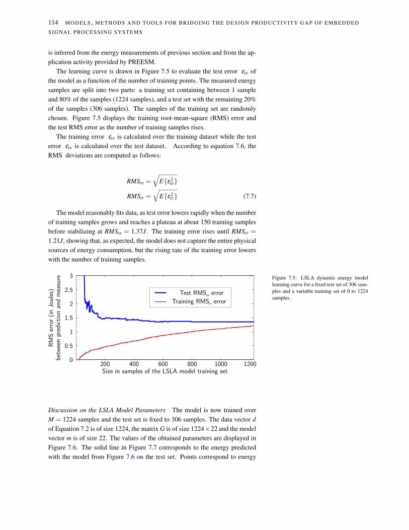
114 MODELS , METHODS AND TOOLS FO R BR IDG ING THE DESI GN PRODUCTI VI TY GA P OF EMBEDDED
SIG NAL PROCESSI NG SY STEMS
is inferred from the energy measurements of previous section and from the ap-
plication activity provided by PREESM.
The learning curve is drawn in Figure 7.5 to evaluate the test error εte of
the model as a function of the number of training points. The measured energy
samples are split into two parts: a training set containing between 1 sample
and 80% of the samples (1224 samples), and a test set with the remaining 20%
of the samples (306 samples). The samples of the training set are randomly
chosen. Figure 7.5 displays the training root-mean-square (RMS) error and
the test RMS error as the number of training samples rises.
The training error εtr is calculated over the training dataset while the test
error εte is calculated over the test dataset. According to equation 7.6, the
RMS deviations are computed as follows:
RMSte =√
E{ε2te}
RMStr =√
E{ε2tr} (7.7)
The model reasonably fits data, as test error lowers rapidly when the number
of training samples grows and reaches a plateau at about 150 training samples
before stabilizing at RMSte = 1.37J. The training error rises until RMStr =
1.21J, showing that, as expected, the model does not capture the entire physical
sources of energy consumption, but the rising rate of the training error lowers
with the number of training samples.
200 400 600 800 1000 12000
0.5
1
1.5
2
2.5
3
RM
Ser
ror
(in
Joule
s)bet
wee
n p
redic
tion
and m
easu
re
Size in samples of the LSLA model training set
Test RMSte error
Training RMStr error
Figure 7.5: LSLA dynamic energy model
learning curve for a fixed test set of 306 sam-
ples and a variable training set of 0 to 1224
samples.
Discussion on the LSLA Model Parameters The model is now trained over
M = 1224 samples and the test set is fixed to 306 samples. The data vector d
of Equation 7.2 is of size 1224, the matrix G is of size 1224×22 and the model
vector m is of size 22. The values of the obtained parameters are displayed in
Figure 7.6. The solid line in Figure 7.7 corresponds to the energy predicted
with the model from Figure 7.6 on the test set. Points correspond to energy

MODELS O F ARCH ITECTU RE IN PRACTI CE 115
-0.551×s+0.010
PE6
PE5 1.232×s+0.119
1.237×s+0.107
PE8
PE7 1.212×s+0.084
1.257×s+0.068
PE2
-1.322×s-0.018
A7CN
PE1
PE3
PE4
1.018×s+0.038
λ=1
0.246×s+0.024
0.230×s+0.048
0.230×s+0.044
0.239×s+0.011
A15CNICC
Figure 7.6: LSLA dynamic energy model
inferred from energy measurements with
computational quanta in ns, communication
quanta in Bytes, and energy data vector d in
nJ. PE1−4 are Cortex-A7 cores and PE5−8 are
Cortex-A15 cores.
samples. The full model offers an energy assessment with a RMSte of 1.37J,
corresponding to an average error of 16%.
config. 1
LSLA predicted costs
median of energy samplesin test set
ener
gy(J
)
30
20
10
0
25
15
5
experiment number0 100 200 300
config. 2 config. 4
config. 5 config. 6
config. 3 Figure 7.7: Comparing the LSLA predicted
cost and the median of the corresponding en-
ergy measurements in test set.
Easily explainable parameters in Figure 7.6 are αPE1to αPE8
because they
translate into average core execution dynamic power, in nJ/ns =W . PEs 1 to
4 have an average dynamic power of 236mW and PEs 5 to 8 have an average
dynamic power of 1.23W . These values are credible and correspond to the
average dynamic powers of a Cortex-A7 core (PEs 1 to 4) and of a Cortex-
A15 core (PEs 5 to 8) running at full speed.
One may observe in Figure 7.7 that the last energy samples of each configu-
ration are lower than their prediction with LSLA. This effect can be explained
by the intra-cluster parallelism that reduces the execution time of the appli-
cation without increasing as much the instantaneous power. This intra-cluster
parallelism tends to decrease the dynamic energy. This effect is partly cap-
tured by the learnt negative costs on internal cluster communication quanta
αA7CN = −1.322nJ/Byte and αA15CN = −0.551nJ/Byte because more paral-
lelism in a cluster leads in general to more communication in this cluster. How-
ever, the amount of communication in a cluster is not fully correlated with the
load balancing inside this cluster, leading to errors. The per-quantum cost of
ICC αICC = 1.018nJ/Byte is positive but, as a token flowing through ICC also
flows through A7CN and A15CN, each inter-cluster exchanged quantum finally

116 MODELS , METHODS AND TOOLS FO R BR IDG ING THE DESI GN PRODUCTI VI TY GA P OF EMBEDDED
SIG NAL PROCESSI NG SY STEMS
costs 1.018−1.322−0.551 =−0.855nJ/Byte. As a consequence, the energy
gain obtained by parallelizing over the whole processor dominates the energy
cost of the communication. This phenomenon motivates for research on a new,
more precise MoA especially capable of capturing the effects of caches.
The LSLA model from Figure 7.6 does not model the mere hardware. In-
stead, it represents hardware together with its operating system, the PREESM
scheduler and the communication and synchronization library. For example,
PREESM tends to favor A15 cores because PREESM optimizes the schedule
for latency and, because A15 cores are much faster than Cortex-A7 cores, the
demand placed on them is greater. An A15 core is less energy efficient than a
Cortex-A7 so the scheduling choices will tend to raise the consumed dynamic
energy.
While the average error of the model is substantial, the built LSLA model is
characterized by an extreme simplicity, the implementation of the cost compu-
tation being reduced to 22 multiplications and a limited number of additions.
Moreover, neither application code nor architecture hardware of low-level rep-
resentation are needed to compute this model cost. Only a MoC and an MoA
are needed, as well as a well defined activity inference method.
Discussion on the Trained LSLA Model Stability In this section, the stability
of the trained LSLA model is tested to account for outliers in training data. To
this end, 100 training sets of size 1224 samples are randomly chosen among
available data, the rest serving as test set. The standard deviations of param-
eters σ(αn) and σ(βn) in the LSLA model, caused by training set modifica-
tions, are reported in Table 7.3. They show that, by far, not all parameters are
equivalent in stability. While parameters αn (applied to quanta) all have mod-
erate standard deviations under 5% (except for A15CN with 7.7%), showing a
rather precise determination, parameters βn (applied to tokens) have in average
standard deviations of 30%. This difference shows that the most stable infor-
mation relevant for energy estimation lies in the number of quanta (in this case,
in the execution time of actors). The number of tokens (number of executed
actors) is less reliably related to energy.
PE/CN PE1 PE2 PE3 PE4 PE5 PE6
αn 0.246 0.230 0.230 0.238 1.239 1.238
σ(αn) 2.9% 3.0% 2.7% 3.0% 0.7% 0.7%
βn 0.027 0.048 0.046 0.012 0.119 0.107
σ(βn) 45.7% 27.3% 23.9% 82.2% 7.1% 6.8%
PE/CN PE7 PE8 A7CN A15CN ICC
αn 1.213 1.258 −1.324 −0.552 1.018
σ(αn) 0.8% 0.6% 1.8% 7.7% 4.6%
βn 0.083 0.068 −0.018 0.010 0.038
σ(βn) 9.2% 13.1% 27.9% 63.1% 16.8%
Table 7.3: Average and standard deviation of
trained LSLA parameters αn and βn when the
training set is varied.

MODELS O F ARCH ITECTU RE IN PRACTI CE 117
Discussion on the Trained LSLA Model Accuracy The RMSte prediction er-
ror of 16% is is provoked by a vast amount of factors, including cache non-
deterministic behaviour, shared memory access arbitration, Linux scheduler
decisions, background tasks, energy measurement sampling effect, etc.
The particular features of the training application (limited parallelism, power
consumed by each actor, correlation between number of tokens and number of
quanta, etc.) make the energy model learning mostly specific, not to one appli-
cation but to a set of applications with similar behavior.
As an example of this specialization, by using LSLA with time quanta to
predict energy, the present analysis assumes the power consumed by a core to
be equivalent for each executed actor. However, it is not the case in reality.
From low-power to high-power actors in the stereo matching application, the
difference of power consumption is +55% on A7 cores and +102% on A15
cores. It is worth noting that the LSLA model averages away most of these
variations on the considered application. However, these variations prevent
from using the same model for predicting the energy of distinct applications.
Characterizing actors with energy and using an activity composed of energy
quanta instead of time quanta is a promising extension for making a single
energy LSLA model usable for different applications.
The fidelity of an LSLA model is certainly more important than its average
error. The next section discusses the fidelity of the inferred LSLA energy
model.
Fidelity of the LSLA Energy Model Model fidelity, as presented in [109],
refers to the probability, for a couple of data di and d j, that the order of the
simulated costs dLSLAi and dLSLA
j matches the order of the measured costs. The
fidelity f of the LSLA energy model is formally defined by
f =2
M(M−1)
M−1
∑i=1
M
∑j=i+1
fi j, (7.8)
where M is the number of measurements and
fi j =
1 if sgn(dLSLAi −dLSLA
j ) = sgn(di −d j)
0 otherwise, (7.9)
with dLSLAi and di respectively the ith LSLA-evaluated and measured energy,
and
sgn(x) =
(−1) if (x < 0)
0 if x = 0
1 if x > 0
. (7.10)
The fidelity of the inferred LSLA model for the considered problem is of
more than 86%, suggesting that the model can be used for taking energy-based

118 MODELS , METHODS AND TOOLS FO R BR IDG ING THE DESI GN PRODUCTI VI TY GA P OF EMBEDDED
SIG NAL PROCESSI NG SY STEMS
decisions at a system level. Fidelity is illustrated by Figure 7.8 where mea-
surements have been sorted in ascending order and are displayed together with
their LSLA prediction.
Simplifying a LSLA Model As explained in Section 7.3.2, different LSLA
topologies can be used to represent a single platform and metric, for example
by merging PEs and CNs. Each cluster of the Exynos 5422 processor having
homogeneous cores, a simplified model of the platform has been experimented
where PEs of one cluster are undifferentiated. As a consequence, only 2 PEs
are retained that each fuse the 4 PEs of one cluster. By doing so, we remove the
cost of intra-cluster communication because the new model does not differen-
tiate intra-core communication from intra-cluster communication. The results
on the same training and test sets of using the simplified model instead of
the original one show a limited degratation of RMStr (1.32J instead of 1.21J)
and RMSte (1.49J instead of 1.21J) and a very slight degradation of fidelity
(85.8% instead of 86.1%). Such a simplification is thus adequate and reduces
cost computation to a set of additions and 6 multiplications.
energy(J)
validation set experiment index after reordering
Ordered energy measurementsCorresponding LSLA energy estimations
50 100 150 200 250 300 3500
5
10
15
20
25
30
0
Figure 7.8: Test set sorted in ascending order
and their corresponding LSLA predictions.
7.4 Conclusions on the Practical Use of MoAs for
Raising System DP
In this chapter, the LSLA Model of Architecture (MoA) has been put into prac-
tice. LSLA represents hardware performance with a linear model, summing
the influences of processing and communication on system efficiency. LSLA
has been demonstrated on an example to predict the dynamic energy of an
MPSoC executing a complex SDF application with a fidelity of 86%. Addi-
tionally, a method for learning the LSLA parameters from hardware measure-
ments has been introduced, automating the creation of the model.

MODELS O F ARCH ITECTU RE IN PRACTI CE 119
LSLA opens new perspectives in building system-level architecture models
that provide reproducible prediction fidelity for a limited complexity.
The example developed in this study is focused on dynamic energy mod-
eling with LSLA for a given operating frequency. A vast amount of potential
extensions exist, defining new models, exploring different NFPs and scaling
up to large numbers of heterogeneous cores. Most of the potential DP gains
are related to predicting the performances of a system to automate decisions.
As a consequence, MoAs will certainly have a key role to play in future im-
provements of DP.


8
Research Perspectives
8.1 Chapter Abstract
This concluding chapter proposes some research directions to continue our
work on improving the DP of DSP systems presented in this report. First, some
achievements are presented that motivate us to propose these new directions
as a continuity of our previous research. Then, the current evolution of DSP
platforms and applications is analyzed and the exposed complexity of embed-
ded DSP architectures, as well as the complexity of applications are shown to
follow an upward trend.
These evolutions motivate for new research on model-based design and
MoAs to focus on the truly relevant parameters when taking system-level deci-
sions. They also motivate us to consider new parameters in automated design
methods such as the relationships between the system and its environment, cap-
tured by the models of Cyber-Physical Systems (CPS). Additionally, if a soft
degradation of applicative QoS can drastically gain performance, it should
also be considered by a design process, as advocated by approximate comput-
ing methods.
Finally, for orders of magnitude of DP to be gained in the next decades,
new rapid prototyping tools will need to be invented that will compile models
of the key non-functional aspects of the system and perform both Design Space
Exploration and functional code generation from a unique set of models. We
intend in the next years to propose models, methods and tools for building this
new generation of DSP system design processes.
8.2 Recent Achievements
This HDR report has covered models, methods and tools for the enhancement
of Design Productivity in DSP systems. A particular focus has been put on the
new concept of Model of Architecture (MoA). Several achievement indicators
encourage us to build on our previously proposed approaches and continue
proposing models and methods for augmenting Design Productivity. We have

122 MODELS , METHODS AND TOOLS FO R BR IDG ING THE DESI GN PRODUCTI VI TY GA P OF EMBEDDED
SIG NAL PROCESSI NG SY STEMS
for instance received the Best Paper awards at the DASIP conference 2014
and 2016 editions and the best demo awards at EDERC 2014 and ICME 2015
respectively for the low energy Open HEVC decoder1 and for the PREESM 1 Erwan Nogues, Morgan Lacour, Erwan Raf-
fin, Maxime Pelcat, and Daniel Menard. Low
power software hevc decoder demo for mo-
bile devices. In Proceedings of the ICME
conference, 2015
tool2. The PREESM website is steadily receiving more than 2500 visits per
2 M. Pelcat, K. Desnos, J. Heulot, C. Guy,
J.-F. Nezan, and S. Aridhi. PREESM: A
dataflow-based rapid prototyping framework
for simplifying multicore dsp programming.
In Proceedings of the EDERC Conference,
Sept 2014
year since 2014. Our book3 has received a positive review by Grant Martin
3 Maxime Pelcat, Slaheddine Aridhi,
Jonathan Piat, and Jean-François Nezan.
Physical Layer Multi-Core Prototyping: A
Dataflow-Based Approach for LTE eNodeB.
Springer, 2012
in IEEE Design and Test [111]. Erwan Nogues has received in 2017 the PhD
award “1er Prix de la Fondation Rennes 1 de l’école doctorale MATISSE”.
Finally, the CERBERO H2020 project, in which INSA Rennes is deeply in-
volved, has been accepted for funding notwithstanding a strong competition
and has started in January 2017. The next section proposes a snapshot of cur-
rent evolutions of DSP embedded systems and the last section exposes research
directions we wish to follow in the next years.
8.3 Current Evolutions in Embedded DSP Systems
8.3.1 More Dynamic and Computation-Intensive Applications
From one generation to the next, signal processing applications gain Quality of
Service (QoS) at the price of additional complexity and, often, of an additional
share of data-dependent processing.
In the video compression domain for instance, the HEVC [70] standard
represents the state-of-the-art of video coding. When compared with the pre-
ceding MPEG Advanced Video Coding (AVC) standard, the HEVC Main pro-
file reduces the bitrate of an encoded video by 40% on average for a similar
objective video quality [112]. The HEVC reference encoder and decoder are
however in average respectively 80% and 60% more complex than the ref-
erence codec of the previous AVC standard [112]. HEVC also comes with
extensive parallelism and much data-dependent processing, caused by a com-
pression method based on the prediction of image blocks from other previously
encoded blocks. Hundreds of different prediction modes are made possible for
a block in order to efficiently reduce block redundancy and, in turn, data rate.
The selection of these modes is based on the processed data and, as a conse-
quence, the amount and type of processing to be executed over time is very
variable. Such variations make multicore load balancing complex and require
runtime execution management such as the one offered by the Spider runtime
and JIT-MS scheduling method (Chapter 2).
Application complexity augmentation applies to all types of DSP process-
ing, from telecommunications to multimedia and from remote sensing to med-
ical appliances. It motivates for DP studies in order for the system price not to
follow the application complexity trend.

RESEAR CH PER SPEC TIVES 123
8.3.2 More Complex Exposed Architectures
Figure 8.1 illustrates different types of recent embedded processor architec-
tures. Most of these processors separate a set of cores dedicated to the con-
trol path and a set of cores or programmable logic dedicated to the data path.
While the control path is responsible for all the decisions in the system —
what, where and when to process — the data path is organized as a stream pro-
cessing pipeline that leverages on data locality to provide good performance-
per-Watt. The energy consumption in systems being largely dominated by data
movements, this heterogeneous system architecture is currently at the heart of
embedded processor energy efficiency.
control path
data pathMulti-ARM GPGPU
Multi-ARM FPGA
Multi-ARM DSP
Multi-Bostan Many-Bostan
a)
b)
c)
d) core
Figure 8.1: Current types of available embed-
ded heterogeneous processor architectures.
Figure 8.1 a) represents the Jetson TX1 module from NVidia that com-
bines a quad-core Cortex-A57 ARM multiprocessor for the control path and
a 256-core Maxwell General Purpose Graphics Processing Unit (GPGPU) for
the data path, organized into 32-core Streaming Multiprocessors (SM). Fig-
ure 8.1 b) represents a Xilinx Virtex Ultrascale+ FPGA that gathers a quad-
core Cortex-A57 ARM multiprocessor and a dual-core low power Cortex-R5
processor together with a large array of programmable logic for the data path.
Figure 8.1 c) represents a 12-core Texas Instruments Keystone II processor
that combines a quad-core Cortex-A15 ARM processor with 8 DSP cores for
the data path. Finally, the Kalray Bostan processor illustrated in Figure 8.1 d)
has quad-core clusters of Kalray Bostan cores for the control path and input-
s/outputs, and 256 Bostan Very Long Instruction Word (VLIW) cores for the
data path. These processors are representative of current high performance
embedded processors.
All the processors illustrated in Figure 8.1 extensively expose complex-
ity and cannot be programmed efficiently without knowing their internal
structure. Apart from the exposed complexity of their heterogeneous cores,
their inter-core interconnects, composed of shared multiport memory banks,
caches, busses, NoCs, switch fabrics, DMAs and interrupt controllers, are also
extremely complex and must be mastered by the system designer for the ob-
tained performance to justify the use of a specific processor.
Adaptable hardware, available in partially reconfigurable FPGA, adds
up to this complexity by introducing a new level of abstraction between tra-
ditional hardware and software. Partially reconfigurable architectures have a
great performance potential due to high versatility combined with a non-Von-
Neumann architecture that removes memory access bottlenecks in the system.

124 MODELS , METHODS AND TOOLS FO R BR IDG ING THE DESI GN PRODUCTI VI TY GA P OF EMBEDDED
SIG NAL PROCESSI NG SY STEMS
However, their Design Productivity is restrained by complex and costly design
and test processes. This restriction could be removed by model-based design
approaches, making partially reconfigurable hardware a prime choice for high
performance processing.
The increasing exposed complexity of embedded hardware architectures in-
volves higher design efforts and amplifies the Design Productivity Gap.
8.4 New Research Directions
So as to further progress in solving the Design Productivity Gap problem, new
models, methods and tools are necessary.
8.4.1 Models
Model-based design is increasingly necessary, as the exposed complexity of
systems rises. A dataflow MoC provides to a compiler or a runtime systems ad-
vanced information on an application state and dependencies. The use of this
information for system NFPs optimizations such as energy efficiency is mostly
unexplored. For instance, the work initiated by Erwan Nogues on dataflow
MoC-based energy optimization4 opens great opportunities for DP improve- 4 Erwan Nogues. Energy optimization of Sig-
nal Processing on MPSoCs and its Applica-
tion to Video Decoding. PhD thesis, INSA de
Rennes, 2016
ments. New evolutions of the PiSDF MoC are also to be envisaged to bet-
ter customize the compromise between application predictability and system
adaptivity. A challenge for application models will be to scale up to the hun-
dreds (and soon thousands) of cores offered by modern architectures. Another
important problem to solve is to mitigate the current limitations of dataflow
MoCs that enforce in-order communication of data tokens in the whole appli-
cation, making the description of some algorithms awkward or even impos-
sible. Relaxing this condition will open many new potential applications to
dataflow-based methods.
Contrary to Models of Computation (MoCs) that have been strongly ex-
plored over the last 3 decades, MoAs constitute a new research field (Chap-
ter 5). We believe that this field will be particularly active in the next few years
and we intend to have a leading role in this evolution. The formal definition of
an MoA proposed in5 is a starting point and much work will be necessary to 5 Maxime Pelcat, Karol Desnos, Luca
Maggiani, Yanzhou Liu, Julien Heulot,
Jean-François Nezan, and Shuvra S
Bhattacharyya. Models of architecture:
Reproducible efficiency evaluation for signal
processing systems. In Proceedings of the
SiPS Workshop. IEEE, 2016
understand the potential of these models, their different forms and their possi-
ble levels of abstraction.
8.4.2 Methods
Considering a system as a CPS makes the environment physical constraints
enter system design. They represent a new level of design automation and new
opportunities of Design Productivity improvements. Within the starting H2020
CERBERO project6, a model-based continuous design method is being built,
6 M. Masin, F. Palumbo, H. Myrhaug, J. A.
de Oliveira Filho, M. Pastena, M. Pelcat,
L. Raffo, F. Regazzoni, A. Sanchez, A. Tof-
fetti, E. de la Torre, and K. Zedda. Cross-
layer design of reconfigurable cyber-physical
systems. Proceedings of the DATE Confer-
ence, 2017
integrating our research results on dataflow-based design methods. We intend

RESEAR CH PER SPEC TIVES 125
to explore forward in the next years the potential of model-based design for
designing CPS.
Approximate computing, consisting in degrading in a controlled way the
Quality of Service (QoS) or a system to dramatically raise its efficiency, is cur-
rently a very active domain. Following the work from Erwan Nogues 7 and the 7 Erwan Nogues, Daniel Menard, and
Maxime Pelcat. Algorithmic-level approxi-
mate computing applied to energy efficient
hevc decoding. IEEE Transactions on
Emerging Topics in Computing, 2016
current PhD of Alexandre Mercat, a vast research field is open, particularly on
using approximate computing for low energy processing. Approximate com-
puting adds a new dimension to the Design Productivity chart where the appli-
cation Quality of Service (QoS) is manipulated together with NRE and NFP
properties. The ARTEFaCT ANR project finances our current research on the
subject.
8.4.3 Tools
A successful example of DP increase is the evolution followed in the last 20
years by Very Long Instruction Word (VLIW) compilers. As VLIW compil-
ers improve, they hide the previously exposed architecture of VLIW cores and
make them transparently programmable by portable code. For example, the
Texas Instruments compiler for C6x cores has hidden most of the VLIW com-
plex internal structure of C6x cores by making it possible to efficiently program
the 8 internal Arithmetic Logic Units (ALUs) of a core from the imperative C
language. Writing assembly code for the C6x core, and thus exposing the
architecture, can still provide execution speedups when compared to C pro-
gramming but these speedups are substancially more limited than in the early
2000s. Importantly, the complexity is resolved at compile time, and thus does
not introduce any runtime management overhead. Such tooling improvement
exemplifies what is needed to augment DPat system level by enabling portable
performances for a unique code executed on different forms of hardware.
However, the optimized performance in VLIW compilers is limited to la-
tency. The situation of embedded system design is much more complicated, as
systems must respects multi-dimensional constraints (time, energy, cost, etc.).
Many innovations will be necessary to provide an acceptable level of code
portability between the previously presented processors. The problem is also
compounded by the complexity of architectures to come, that are forecast to
expose even more complexity than today’s architectures.
A promising approach for gaining orders of magnitude of Design Produc-
tivity is rapid prototyping. A rapid prototyping tool is composed of a Design
Space Exploration (DSE) process and a functional code generation. While the
DSE process [99] performs high-level multi-dimensional optimization, tak-
ing into account both “cyber” and physical system information, as well as a
set of system relevant Non-Functional Properties (NFPs), the functional code
generation produces system design information compatible with lower-level
compilers. Exploring the design space consists in creating a Pareto chart such
as the one in Figure 8.2 and choosing solutions on the Pareto front, i.e. solu-

126 MODELS , METHODS AND TOOLS FO R BR IDG ING THE DESI GN PRODUCTI VI TY GA P OF EMBEDDED
SIG NAL PROCESSI NG SY STEMS
tions that represent the best alternative in at least one dimension and respect
constraints in the other dimensions. As an example, p1 on Figure 8.2 may be
energy consumption and p2 may represent the response time to input data. Fig-
ure 8.2 illustrates in 2 dimensions a problem that, in general, has many more
dimensions.
better p1
better p2
worse p1
worse p2
constraint on maximum p1
Pareto curve and
Pareto-optimal points
explored system
with sub-optimal efficiency
non-achieved efficiency
Figure 8.2: The problem of Design Space Ex-
ploration (DSE) illustrated on a 2-D Pareto
chart with efficiency metrics p1 and p2.
Using rapid prototyping for gaining productivity by raising the abstraction
of compiler models is one of our motivations for proposing the new domain
of MoAs. Indeed, separating the application concern (modeled by a MoC) and
architecture concern (modeled by an MoA) makes it possible to generate many
points for the DSE Pareto by separately varying application and architecture
parameters and observing their effects on system efficiency. For example, the
designer can build an application, test its efficiency on different platform ar-
chitectures and, if constraints are not met by any point on the Pareto, iterate
this process until reaching a satisfactory efficiency. This process is illustrated
on Figure 8.3 and leads to the Pareto points from Figure 8.2. The more a rapid
prototyping tool can, by itself, play with application and architecture parame-
ters, the better the resulting DP should be.
Tools also need to enter designers’ best practices at a higher pace than
today. On the hardware design side for example, the VHDL, Verilog and
SystemVerilog most commonly used languages for logic synthesis today are
progressively complemented with High-Level Synthesis (HLS) languages such
as C or OpenCL (Chapter 4). However, between the creation of the first C-
based HLS methods and the beginning of broad adoption, more than 30 years
have passed [65], equivalent in technological years to a geological era. For
speeding up the introduction of future model-based design tools, we intend to
continue our efforts on fair DP evaluation that provide in-depth information
on what makes a method higher-level than another(Chapter 4).
The privileged subjects for our future research are illustrated in Figure 8.4.
Future studies on model-based approaches, approximate computing, cyber-
physical systems and rapid prototyping will need to follow the rapid — and
hardly predictable — evolution of applications and platforms. In particular,
with the exponential expansion of artificial intelligence applications, an in-
flexion is likely to be observed in the next years on processor architectural

RESEAR CH PER SPEC TIVES 127
iterations on application design
iterations on architecture design
system design
redesign
application
redesign
application
constraints
not met
constraints
not met
constraints
met
mapping
application
to different
architectures
system
efficiency
to be assessed
with N-D Pareto
curve
redesign architecture redesign architecture
affect QoS & efficiency
affect efficiency
MoC
MoA
Figure 8.3: Example of an iterative design
process where application is refined and, for
each refinement step, tested with a set of
architectures to generate new points for the
Pareto chart.
choices. Moreover, hardware partial reconfiguration will certainly become a
standard feature and may provoke a spectacular establishment of virtualization
into the hardware world. Finally, the Internet of Things (IoT) and Internet of
Everything (IoE) trends are fostering interconnected systems with collective
intelligence. These subjects are at the heart of the current PhD thesis of Kamel
Abdelouahab, El Mehdi Abdali, Jonathan Bonnard and Alexandre Mercat, and
I am proud and happy to participate to this dynamic research process.
Ever more complex
and variable applications
Ever increasing
exposed architecture complexity
Growing Design Productivity Gap
Slow tool adoption
Approximate Computing
Fair Design Productivity Evaluation
Cyber-Physical SystemsModels of Architecture
Rapid Prototyping
Embedded systems' evolution Next research subjects
motivates
Figure 8.4: Priviledged next research sub-
jects.


Bibliography
[1] Maxime Pelcat, Cédric Bourrasset, Luca Maggiani, and François Berry.
Design productivity of a high level synthesis compiler versus HDL. In
Proceedings of IC-SAMOS, 2016.
[2] Maxime Pelcat, Karol Desnos, Luca Maggiani, Yanzhou Liu, Julien
Heulot, Jean-François Nezan, and Shuvra S Bhattacharyya. Models of
architecture: Reproducible efficiency evaluation for signal processing
systems. In Proceedings of the SiPS Workshop. IEEE, 2016.
[3] Mont-Blanc European projects.
[4] International technology roadmap for semiconductors - executive sum-
mary, 2011.
[5] International technology roadmap for semiconductors - executive re-
port, 2015.
[6] M. Pelcat, K. Desnos, J. Heulot, C. Guy, J.-F. Nezan, and S. Aridhi.
PREESM: A dataflow-based rapid prototyping framework for simplify-
ing multicore dsp programming. In Proceedings of the EDERC Confer-
ence, Sept 2014.
[7] Julien Heulot, Maxime Pelcat, Karol Desnos, Jean François Nezan, Sla-
heddine Aridhi, et al. SPIDER: A synchronous parameterized and in-
terfaced dataflow-based rtos for multicore dsps. Proceedings of the ED-
ERC Conference, 2014.
[8] K. Desnos, M. Pelcat, J.-F. Nezan, S. S. Bhattacharyya, and S. Aridhi.
PiMM: Parameterized and interfaced dataflow meta-model for MPSoCs
runtime reconfiguration. In SAMOS XIII, 2013.
[9] J. Piat, S.S. Bhattacharyya, and M. Raulet. Interface-based hierarchy for
synchronous data-flow graphs. In Proceedings of the SiPS Workshop,
2009.
[10] B.D. Theelen, MCW Geilen, T. Basten, JPM Voeten, S.V. Gheorghita,
and S. Stuijk. A scenario-aware dataflow model for combined long-run
average and worst-case performance analysis. In MEMOCODE, 2006.

130 MODELS , METHODS AND TOOLS FO R BR IDG ING THE DESI GN PRODUCTI VI TY GA P OF EMBEDDED
SIG NAL PROCESSI NG SY STEMS
[11] Maxime Pelcat, Slaheddine Aridhi, Jonathan Piat, and Jean-François
Nezan. Physical Layer Multi-Core Prototyping: A Dataflow-Based Ap-
proach for LTE eNodeB. Springer, 2012.
[12] H. Nikolov, T. Stefanov, and E. Deprettere. Modeling and FPGA imple-
mentation of applications using parameterized process networks with
non-static parameters. In FCCM Proceedings, 2005.
[13] Edward Lee and Thomas M Parks. Dataflow process networks. Pro-
ceedings of the IEEE, 1995.
[14] E.A. Lee and T.M. Parks. Dataflow process networks. Proceedings of
the IEEE, 1995.
[15] B. Bhattacharya and S.S. Bhattacharyya. Parameterized dataflow mod-
eling for dsp systems. Signal Processing, IEEE Transactions on, 2001.
[16] E. A. Lee and D. G. Messerschmitt. Synchronous data flow. Proceed-
ings of the IEEE, 1987.
[17] G. Bilsen, M. Engels, R. Lauwereins, and J. Peperstraete. Cyclo-static
dataflow. Signal Processing, IEEE Transactions on, 1996.
[18] P.K. Murthy and E.A. Lee. Multidimensional synchronous dataflow.
Signal Processing, IEEE Transactions on, 2002.
[19] Adnan Bouakaz, Jean-Pierre Talpin, and Jan Vitek. Affine data-flow
graphs for the synthesis of hard real-time applications. ACSD, 2012.
[20] Joost P.H.M. Hausmans, Stefan J. Geuns, Maarten H. Wiggers, and
Marco J.G. Bekooij. Compositional temporal analysis model for in-
cremental hard real-time system design. In EMSOFT ’12 Proceedings,
2012.
[21] J.S. Ostroff. Abstraction and composition of discrete real-time systems.
Proc. of CASE, 1995.
[22] S. Neuendorffer and E. Lee. Hierarchical reconfiguration of dataflow
models. In Proceedings of MEMOCODE Conference. IEEE, 2004.
[23] Julien Heulot, Maxime Pelcat, Jean-François Nezan, Yaset Oliva, Sla-
heddine Aridhi, and Shuvra S Bhattacharyya. Just-in-time scheduling
techniques for multicore signal processing systems. In Proceedings of
the GlobalSIP conference. IEEE, 2014.
[24] Texas Instruments. Multicore Fixed and Floating-Point Digital Signal
Processor - SPRS691E.
[25] Kalray. MPPA MANYCORE: a multicore processors family.
[26] Adapteva. Epiphany: A breakthrough in parallel processing.

BI BLIO GRAPH Y 131
[27] Philipp Helle, Haricharan Lakshman, Mischa Siekmann, Jan Stege-
mann, Tobias Hinz, Heiko Schwarz, Detlev Marpe, and Thomas Wie-
gand. A scalable video coding extension of HEVC. In Data Compres-
sion Conference (DCC), 2013, 2013.
[28] P. Marwedel, J. Teich, G. Kouveli, I. Bacivarov, L. Thiele, S. Ha, C. Lee,
Q. Xu, and L. Huang. Mapping of applications to MPSoCs. In Proceed-
ings of the CODES+ISSS conference. ACM, 2011.
[29] E. Lee and S. Ha. Scheduling strategies for multiprocessor real-time
dsp. In Proceedings of the GLOBECOM conference. IEEE, 1989.
[30] Amit Kumar Singh, Muhammad Shafique, Akash Kumar, and Jörg
Henkel. Mapping on multi/many-core systems: Survey of current and
emerging trends. In Proceedings of the DAC conference. ACM, 2013.
[31] Leonardo Dagum and Ramesh Menon. OpenMP: an industry standard
api for shared-memory programming. Computational Science & Engi-
neering, IEEE, 1998.
[32] John E Stone, David Gohara, and Guochun Shi. Opencl: A parallel pro-
gramming standard for heterogeneous computing systems. Computing
in science & engineering, 2010.
[33] George F Zaki, William Plishker, Shuvra S Bhattacharyya, Charles
Clancy, and John Kuykendall. Integration of dataflow-based hetero-
geneous multiprocessor scheduling techniques in gnu radio. Journal of
Signal Processing Systems, 2013.
[34] S. Sriram and S. S. Bhattacharyya. Embedded multiprocessors:
Scheduling and synchronization. CRC press, 2012.
[35] Yu-Kwong Kwok. High-performance algorithms for compile-time
scheduling of parallel processors. Ph. D. thesis, 1997.
[36] Edward Lee and David G. Messerschmitt. Static scheduling of syn-
chronous data flow programs for digital signal processing. Computers,
IEEE Transactions on, 1987.
[37] Jani Boutellier, Shuvra S Bhattacharyya, and Olli Silvén. A low-
overhead scheduling methodology for fine-grained acceleration of sig-
nal processing systems. Journal of Signal Processing Systems, 2010.
[38] Texas Instruments. KeyStone Architecture Multicore Navigator.
[39] Julien Heulot. Runtime multicore scheduling techniques for dispatch-
ing parameterized signal and vision dataflow applications on heteroge-
neous MPSoCs. PhD thesis, INSA Rennes, 2015.

132 MODELS , METHODS AND TOOLS FO R BR IDG ING THE DESI GN PRODUCTI VI TY GA P OF EMBEDDED
SIG NAL PROCESSI NG SY STEMS
[40] Zheng Zhou, William Plishker, Shuvra S Bhattacharyya, Karol Desnos,
Maxime Pelcat, and Jean-Francois Nezan. Scheduling of parallelized
synchronous dataflow actors for multicore signal processing. Journal
of Signal Processing Systems, 2016.
[41] Manel Ammar, Mouna Baklouti, Maxime Pelcat, Karol Desnos, and
Mohamed Abid. Marte to πsdf transformation for data-intensive appli-
cations analysis. In Proceedings of the DASIP Conference. IEEE, 2014.
[42] Karol Desnos. Memory Study and Dataflow Representations for Rapid
Prototyping of Signal Processing Applications on MPSoCs. PhD thesis,
INSA Rennes, 2014.
[43] Karol Desnos, Maxime Pelcat, Jean François Nezan, and Slaheddine
Aridhi. Memory Bounds for the Distributed Execution of a Hierarchi-
cal Synchronous Data-Flow Graph. In Proceedings of the IC-SAMOS
Conference, 2012.
[44] Jonathan Piat. Data flow modelling and optimization of loops for multi-
core architectures. PhD thesis, INSA de Rennes, 2010.
[45] Karol Desnos, Maxime Pelcat, Jean François Nezan, and Slaheddine
Aridhi. Pre- and post-scheduling memory allocation strategies on MP-
SoCs. In Proceedings of the ESLsyn conference, 2013.
[46] Karol Desnos, Maxime Pelcat, Jean-François Nezan, and Slaheddine
Aridhi. Memory Analysis and Optimized Allocation of Dataflow Ap-
plications on Shared-Memory MPSoCs. Journal of VLSI Signal Pro-
cessing Systems for Signal, Image, and Video Technology (JSPS), 2014.
[47] Karol Desnos, Maxime Pelcat, Jean-François Nezan, and Slaheddine
Aridhi. Buffer Merging Technique for Minimizing Memory Footprints
of Synchronous Dataflow Specifications. In Proceedings of the ICASSP
Conference, 2015.
[48] Karol Desnos, Maxime Pelcat, Jean François Nezan, and Slaheddine
Aridhi. On Memory Reuse Between Inputs and Outputs of Dataflow
Actors. ACM Transactions on Embedded Computing Systems (TECS),
2016.
[49] Karol Desnos, Maxime Pelcat, Jean-François Nezan, and Slaheddine
Aridhi. Distributed memory allocation technique for synchronous
dataflow graphs. In Proceedings of the SiPS Workshop. IEEE, 2016.
[50] Trevor Mudge. Computer power: A first-class architectural design con-
straint. IEEE Computer Magazine, 2001.
[51] Simon Holmbacka, Erwan Nogues, Maxime Pelcat, Sébastien Lafond,
and Johan Lilius. Energy efficiency and performance management of

BI BLIO GRAPH Y 133
parallel dataflow applications. In Proceedings of the DASIP conference.
IEEE, 2014.
[52] Simon Holmbacka, Erwan Nogues, Maxime Pelcat, Sébastien Lafond,
Daniel Menard, and Johan Lilius. Energy-awareness and performance
management with parallel dataflow applications. Journal of Signal Pro-
cessing Systems, 2015.
[53] Erwan Nogues. Energy optimization of Signal Processing on MPSoCs
and its Application to Video Decoding. PhD thesis, INSA de Rennes,
2016.
[54] David G Luenberger. Optimization by vector space methods. John Wi-
ley & Sons, 1969.
[55] Erwan Nogues, Julien Heulot, Glenn Herrou, Ladislas Robin, Maxime
Pelcat, Daniel Menard, Erwan Raffin, and Wassim Hamidouche. Effi-
cient DVFS for low power HEVC software decoder. Journal of Real-
Time Image Processing, 2016. Springer Verlag.
[56] Alexandre Mercat, Wassim Hamidouche, Maxime Pelcat, and Daniel
Menard. Estimating encoding complexity of a real-time embedded soft-
ware hevc codec. In Proceedings of the DASIP conference. IEEE, 2016.
[57] Alexandre Mercat, Florian Arrestier, Wassim Hamidouche, Maxime
Pelcat, and Daniel Menard. Energy reduction opportunities in an hevc
real-time encoder. In Proceedings of the ICASSP conference, 2017.
[58] Alexandre Mercat, Florian Arrestier, Wassim Hamidouche, Maxime
Pelcat, and Daniel Menard. Constrain the docile ctus: an in-frame com-
plexity allocator for hevc intra encoders. In Proceedings of the ICASSP
conference, 2017.
[59] Karol Desnos, Safwan El Assad, Aurore Arlicot, Maxime Pelcat, and
Daniel Menard. Efficient multicore implementation of an advanced
generator of discrete chaotic sequences. In Proceedings of the ICITST
conference, pages 31–36. IEEE, 2014.
[60] Raquel Lazcano, Daniel Madroñal, Karol Desnos, Maxime Pelcat, Raúl
Guerra, Sebastián López, Eduardo Juarez, and César Sanz. Parallelism
Exploitation of a Dimensionality Reduction Algorithm Applied to Hy-
perspectral Images. In Proceedings of the DASIP Conference, 2016.
[61] Erwan Raffin, Erwan Nogues, Wassim Hamidouche, Seppo Tomperi,
Maxime Pelcat, and Daniel Menard. Low power hevc software decoder
for mobile devices. Journal of Real-Time Image Processing, 2016.
[62] Carlo Sau, Francesca Palumbo, Maxime Pelcat, Julien Heulot, Erwan
Nogues, Daniel Ménard, Paolo Meloni, and Luigi Raffo. Challenging

134 MODELS , METHODS AND TOOLS FO R BR IDG ING THE DESI GN PRODUCTI VI TY GA P OF EMBEDDED
SIG NAL PROCESSI NG SY STEMS
the best HEVC fractional pixel FPGA interpolators with reconfigurable
and multi-frequency approximate computing. IEEE Embedded Systems
Letters, 2017. IEEE, to appear.
[63] Jinglin Zhang, Jean-Francois Nezan, Maxime Pelcat, and Jean-Gabriel
Cousin. Real-time gpu-based local stereo matching method. In Pro-
ceedings of the DASIP Conference. IEEE, 2013.
[64] Kamel Abdelouahab, Cédric Bourrasset, Maxime Pelcat, François
Berry, Jean-Charles Quinton, and Jocelyn Serot. A holistic approach
for optimizing dsp block utilization of a cnn implementation on fpga.
In Proceedings of the ICDSC Conference. ACM, 2016.
[65] Grant Martin and Gary Smith. High-level synthesis: Past, present, and
future. IEEE Design & Test of Computers, 2009.
[66] Haoxing Ren. A brief introduction on contemporary high-level synthe-
sis. In 2014 IEEE International Conference on IC Design & Technol-
ogy, 2014.
[67] Johan Eker and J Janneck. Cal language report: Specification of the cal
actor language, 2003.
[68] J. Sérot and F. Berry. High-level dataflow programming for reconfig-
urable computing. In Proceedings of the SBAC-PAD Workshop, 2014.
[69] Synflow. The Cx programming language. http://cx-lang.org,
2015. Accessed: 2015-09-25.
[70] Gary J Sullivan, Jens Ohm, Woo-Jin Han, and Thomas Wiegand.
Overview of the high efficiency video coding (hevc) standard. IEEE
Transactions on circuits and systems for video technology, 2012.
[71] Oleg Grodzevich and Oleksandr Romanko. Normalization and other
topics in multi-objective optimization. In Proceedings of the Fields -
MITACS Industrial Problems Workshop, 2006.
[72] Merwan Birem and François Berry. Dreamcam: A modular fpga-based
smart camera architecture. Journal of Systems Architecture, 2014.
[73] Volnei Pedroni. Circuit design with VHDL. MIT press, 2004.
[74] B. Kienhuis, E. Deprettere, K. Vissers, and P. van der Wolf. An ap-
proach for quantitative analysis of application-specific dataflow archi-
tectures. In Proceedings of the ASAP Conference. IEEE, 1997.
[75] Texas Instruments. 66AK2L06 Multicore DSP+ARM KeyStone II
System-on-Chip (SoC) - SPRS930. Texas Instruments, 2015.
[76] Ashley Stevens. Introduction to amba 4 ace and big.little processing
technology, 2011.

BI BLIO GRAPH Y 135
[77] J. Eker, J. W Janneck, E. Lee, J. Liu, X. Liu, J. Ludvig, S. Neuendorffer,
S. Sachs, Y. Xiong, et al. Taming heterogeneity-the ptolemy approach.
Proceedings of the IEEE, 2003.
[78] Fabrice Bellard. QEMU, a Fast and Portable Dynamic Translator. In
USENIX Annual Technical Conference, FREENIX Track, 2005.
[79] Nathan Binkert, Bradford Beckmann, Gabriel Black, Steven K. Rein-
hardt, Ali Saidi, Arkaprava Basu, Joel Hestness, Derek R. Hower,
Tushar Krishna, Somayeh Sardashti, and others. The gem5 simulator.
ACM SIGARCH Computer Architecture News, 2011.
[80] B. Kienhuis, E. F. Deprettere, P. Van Der Wolf, and K. Vissers. A
methodology to design programmable embedded systems. In Embed-
ded processor design challenges. Springer, 2002.
[81] Maxime Pelcat. Models of Architecture for DSP Systems. In Shuvra S
Bhattacharyya, Ed F Deprettere, Rainer Leupers, and Jarmo Takala, ed-
itors, Handbook of signal processing systems, third edition. Springer
Science & Business Media, to appear, 2017.
[82] Peter H Feiler and David P Gluch. Model-based engineering with
AADL: an introduction to the SAE architecture analysis & design lan-
guage. Addison-Wesley, 2012.
[83] SAE International. Architecture analysis and design language (aadl) -
http://standards.sae.org/as5506c/ (accessed 03/2017), 2012.
[84] Gilles Lasnier, Bechir Zalila, Laurent Pautet, and Jérome Hugues. Oca-
rina: An environment for aadl models analysis and automatic code gen-
eration for high integrity applications. In International Conference on
Reliable Software Technologies. Springer, 2009.
[85] P. H. Feiler, D. P. Gluch, and J. J. Hudak. The architecture analysis
& design language (AADL): An introduction. Technical report, DTIC
Document, 2006.
[86] Morten Larsen. Modelling field robot software using aadl. Technical
Report Electronics and Computer Engineering, 2016.
[87] Maxime Pelcat, Alexandre Mercat, Karol Desnos, Luca Maggiani,
Yanzhou Liu, Julien Heulot, Jean-François Nezan, Wassim Hami-
douche, Daniel Menard, and Shuvra S Bhattacharyya. Models of Ar-
chitecture: Application to ESL Model-Based Energy Consumption Es-
timation. Research report, IETR/INSA Rennes ; Scuola Superiore
Sant’Anna, Pisa ; Institut Pascal ; University of Maryland, College Park
; Tampere University of Technology, Tampere, 2017.
[88] Edward A Lee. The problem with threads. Computer, 2006.
136 MODELS , METHODS AND TOOLS FO R BR IDG ING THE DESI GN PRODUCTI VI TY GA P OF EMBEDDED
SIG NAL PROCESSI NG SY STEMS
[89] Peter Van Roy et al. Programming paradigms for dummies: What every
programmer should know. New computational paradigms for computer
music, 2009.
[90] Masaki Gondo, Fumio Arakawa, and Masato Edahiro. Establishing a
standard interface between multi-manycore and software tools-SHIM.
In COOL Chips XVII, 2014 IEEE. IEEE, 2014.
[91] Multicore Association. Software/Hardware Interface
for Multicore/Manycore (SHIM) - http://www.multicore-
association.org/workgroup/shim.php/ (accessed 03/2017), 2015.
[92] Chris Lattner and Vikram Adve. LLVM: A compilation framework for
lifelong program analysis & transformation. In Proceedings of the in-
ternational symposium on Code generation and optimization: feedback-
directed and runtime optimization. IEEE Computer Society, 2004.
[93] OMG. UML Profile for MARTE: Modeling and Analysis of Real-Time
Embedded Systems. Object Management Group, 2011.
[94] Madeleine Faugere, Thimothee Bourbeau, Robert De Simone, and Se-
bastien Gerard. Marte: Also an uml profile for modeling aadl appli-
cations. In Engineering Complex Computer Systems, 2007. 12th IEEE
International Conference on. IEEE, 2007.
[95] Frédéric Mallet and Charles André. UML/MARTE CCSL, signal and
petri nets. PhD thesis, INRIA, 2008.
[96] Frédéric Mallet and Robert De Simone. Marte vs. aadl for discrete-
event and discrete-time domains. In Languages for Embedded Systems
and Their Applications. Springer, 2009.
[97] Thierry Grandpierre and Yves Sorel. From algorithm and architecture
specifications to automatic generation of distributed real-time execu-
tives: a seamless flow of graphs transformations. In Proceedings of the
MEMOCODE conference. ACM/IEEE, 2003.
[98] V. Kianzad and S. S. Bhattacharyya. CHARMED: A multi-objective
co-synthesis framework for multi-mode embedded systems. In
Application-Specific Systems, Architectures and Processors, 2004. Pro-
ceedings. 15th IEEE International Conference on. IEEE, 2004.
[99] Andy D. Pimentel. Exploring exploration: A tutorial introduction to
embedded systems design space exploration. IEEE Design & Test,
2017.
[100] M. Pelcat, J.-F. Nezan, J. Piat, Jerome Croizer, and S. Aridhi. A system-
level architecture model for rapid prototyping of heterogeneous multi-
core embedded systems. In Proceedings of DASIP conference, 2009.

BI BLIO GRAPH Y 137
[101] Manel Ammar, Mouna Baklouti, Maxime Pelcat, Karol Desnos, and
Mohamed Abid. Automatic generation of s-lam descriptions from um-
l/marte for the dse of massively parallel embedded systems. In Soft-
ware Engineering, Artificial Intelligence, Networking and Parallel/Dis-
tributed Computing 2015. Springer, 2016.
[102] J. Castrillon Mazo and R. Leupers. Programming Heterogeneous MP-
SoCs. Springer International Publishing, Cham, 2014.
[103] Gilles Kahn. The semantics of a simple language for parallel program-
ming. In Information Processing, 1974.
[104] Brice Goglin. Managing the topology of heterogeneous cluster nodes
with hardware locality (hwloc). In High Performance Computing &
Simulation (HPCS), 2014 International Conference on. IEEE, 2014.
[105] R. C Aster, B. Borchers, and C. H Thurber. Parameter estimation and
inverse problems. Academic Press, 2011.
[106] Douglas C Montgomery, Elizabeth A Peck, and G Geoffrey Vining.
Introduction to linear regression analysis. John Wiley & Sons, 2015.
[107] A. Mercat, J.-F. Nezan, D. Menard, and J. Zhang. Implementation of
a stereo matching algorithm onto a manycore embedded system. In
Proceedings of the ISCAS conference. IEEE, 2014.
[108] K. Desnos and J. Zhang. PREESM project - stereo matching, 2017.
svn://svn.code.sf.net/p/preesm/code/trunk/tests/stereo.
[109] N. K. Bambha and S. S. Bhattacharyya. A joint power/performance op-
timization algorithm for multiprocessor systems using a period graph
construct. In Proceedings of the 13th international symposium on Sys-
tem synthesis. IEEE Computer Society, 2000.
[110] Erwan Nogues, Morgan Lacour, Erwan Raffin, Maxime Pelcat, and
Daniel Menard. Low power software hevc decoder demo for mobile
devices. In Proceedings of the ICME conference, 2015.
[111] Grant Martin. Let’s get physical [review of" physical layer multi-core
prototyping: A dataflow-based approach for lte enodeb"]. IEEE Design
& Test, 2014.
[112] Jarno Vanne, Marko Viitanen, Timo D Hamalainen, and Antti Halla-
puro. Comparative rate-distortion-complexity analysis of hevc and avc
video codecs. IEEE Transactions on Circuits and Systems for Video
Technology, 2012.
[113] M. Masin, F. Palumbo, H. Myrhaug, J. A. de Oliveira Filho, M. Pastena,
M. Pelcat, L. Raffo, F. Regazzoni, A. Sanchez, A. Toffetti, E. de la

138 MODELS , METHODS AND TOOLS FO R BR IDG ING THE DESI GN PRODUCTI VI TY GA P OF EMBEDDED
SIG NAL PROCESSI NG SY STEMS
Torre, and K. Zedda. Cross-layer design of reconfigurable cyber-
physical systems. Proceedings of the DATE Conference, 2017.
[114] Erwan Nogues, Daniel Menard, and Maxime Pelcat. Algorithmic-
level approximate computing applied to energy efficient hevc decoding.
IEEE Transactions on Emerging Topics in Computing, 2016.