models of visual neuron function - cornell...

Models of visual neuron function

Quantitative Biology Course LectureDan Butts

1

12

10 neurons

1,000-10,000 inputs

Electrical activity: nerve impulses

11

What is the “neural code"?

2

12

How does neural activity relate to brain function?

?

Well characterized

Intuitive functionUse visual system:

Lateral Geniculate Nucleus(LGN) Population input to the cortex

3

The Visual Cortex

Lateral Geniculate Nucleus(LGN)

Starting point: recordings in the LGN

Retina

Extracellular recordings (Jose-Manuel Alonso Lab)

1. Still relatively simple non-linear transforms on stimulus

2. Population input to the visual cortex

4

Visual stimulus

“Cat-cam” movies from Peter

Koenig’s Lab

(Kayser et al, 2004)5

500 ms

LGN neuron responses

6

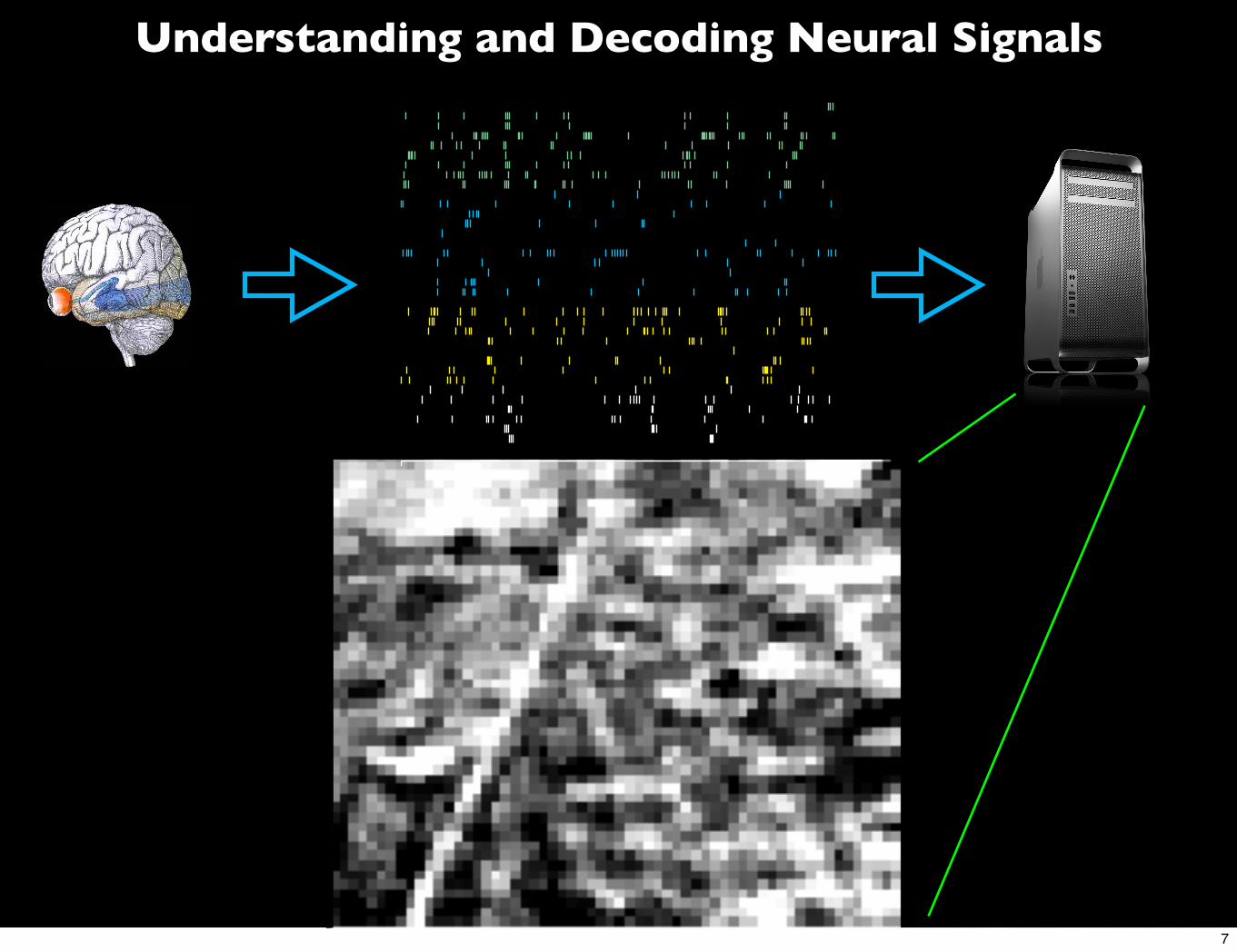
Understanding and Decoding Neural Signals

7

Outline1. Introduction to “receptive fields”

2. Building a visual neuron model

3. The problem of temporal precision and the need for new statistical methods

4. Research: Application of maximum-likelihood modeling to explain precise timing of neuronal responses

The LN (Linear-Non-linear) model

Maximum-likelihood modeling

8

Coding like the muscle

Muscle picturewith motoneuron

Littlecontraction

Lots ofcontraction

9

LGN

The receptive field

Spatial receptive field

Retina

LGN responses related to how much the stimulus matches the

receptive field

+

Center Surr.

RF

Stim

+ -

Linear comparison:R =

!

!x

Ksp(!x) S(!x)

+

+ -

+ +

Multiplication

+

Spatial stimulus

10

LGN

The receptive field


Retina

+

Center Surr.

RF

Stim

+ -

+

+

+

Multiplication

0 -

Linear comparison:R =

!

!x

Ksp(!x) S(!x)

LGN responses related to how much the stimulus matches the

receptive field

Spatial stimulus

11

LGN

The receptive field


Retina

Spatial features of image matter in relation to RF

++

Center Surr.

RF

Stim

+ --

-

+

Multiplication

- -

Neuron is tuned for a given stimulus over a certain range.Spatial stimulus

12

Circuitry of the retina

13

...but vision involves motion

Motion in thevisual scene/self motion

Eye movements• saccades, microsac.• ocular drift

14

1.2 1.6 2.0 2.4 2.80

50

100

Time (sec)

Fir

ing R

ate

(H

z)

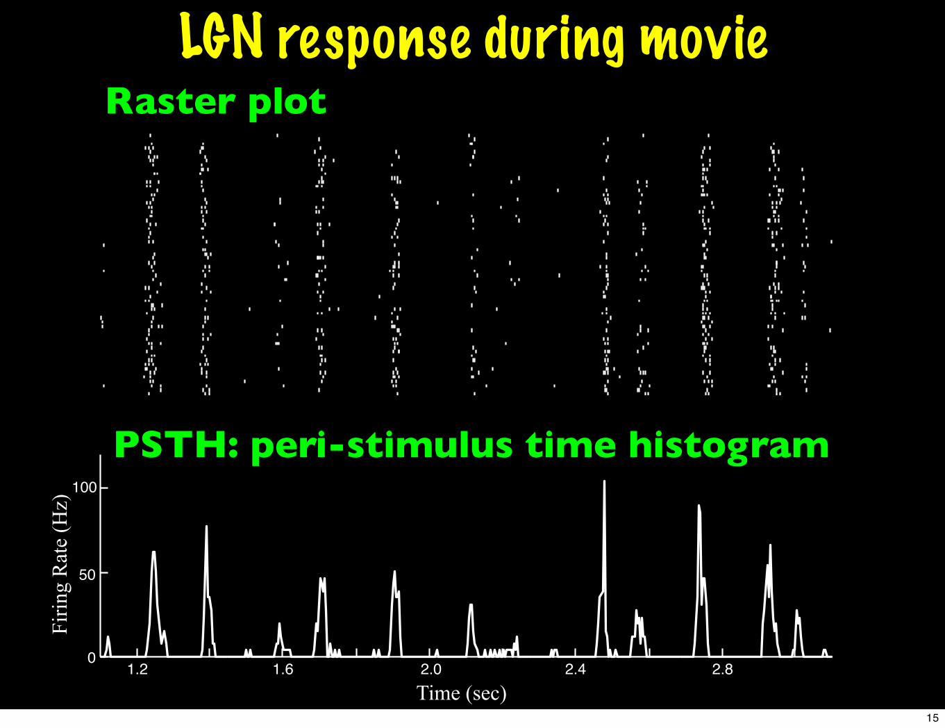
PSTH: peri-stimulus time histogram

LGN response during movieRaster plot

15

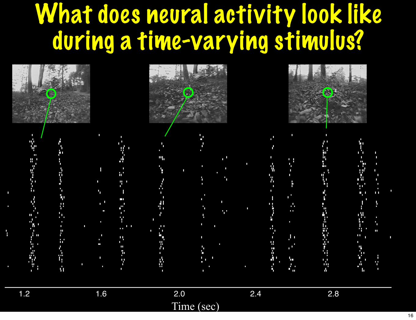
Raster Plot

1.2 1.6 2.0 2.4 2.8Time (sec)

What does neural activity look like during a time-varying stimulus?

16

Visual neuron function: the spatiotemporal receptive field

What stimuli are represented by a neuron’s response?

Spike-Triggered Average (STA)stimulus: “receptive field”

-200 ms -100

17

Visual neuron function: the spatiotemporal receptive field

What stimuli are represented by a neuron’s response?

Spike-Triggered Average (STA)stimulus: “receptive field”

-200 ms -100

18

Implicit Problems with Modeling> Too many parameters

0 5 10 15 20 25!0.4

!0.3

!0.2

!0.1

0

0.1

0.2

0.3

0.4

0.5

0.6

5 10 15 20 25 30

5

10

15

20

25

30 !0.04

!0.03

!0.02

!0.01

0

0.01

0.02

0.03

5 10 15 20 25 30

5

10

15

20

25

30

!0.04

!0.02

0

0.02

0.04

0.06

0.08

0.1

0.12

0.14

5 10 15 20 25 30

5

10

15

20

25

300

0.1

0.2

0.3

0.4

0.5

5 10 15 20 25 30

5

10

15

20

25

30 !0.3

!0.25

!0.2

!0.15

!0.1

!0.05

0

5 10 15 20 25 30

5

10

15

20

25

30 !0.04

!0.03

!0.02

!0.01

0

0.01

0.02

0.03

0.04

19

-100

Time (ms)

Averag

e tempo

ral stim

Full-field stimuli

-100

Time (ms)

Av

erage tem

po

ral stim

Spatiotemporal Stimuli

The “temporal receptive field”

20







21

Full-field stimuli

-100

Time (ms)

Av

erage tem

poral stim

The “temporal receptive field”

22

How measure the receptive field?The spike-triggered average

Full-field stimuli

-100

Time (ms)

Av

erage tem

po

ral stim

k(!) !!

dt r(t) s(t" !)

Stimulus-response cross-correlation

23

100 150 200 250 ms

Temporal Stimulus(full-field)

Filteredstimulus

x

=Temporal

Receptive Field

Linear model predictions

rest(t) = r0 +!

d! k(!) s(t! !)

24

Mathematical result

Layman’s summary:In the presence of Gaussian noise (uncorrelated) stimuli, the best linear model for the neuron is proportional to the spike triggered average.

(take functional derivative of MSE)

rest(t) = r0 +!

d! k(!) s(t! !)

k(!) !!

dt r(t) s(t" !)

Stimulus-response cross-correlationMean Squared Error (MSE)

MSE =!

t

[r(t)! rest(t)]2

25

100 150 200 250 ms


Filteredstimulus

x

=Temporal

Receptive Field

Linear model predictions

Firin

g R

ate

Observed firing rate

100 150 200 250 ms

0

500

Hz

26

How map linear function to firing rate?

Firin

g R

ate

Observed firing rate

100 150 200 250 ms

0

500

Hz

inear Kernel

Stimulus s(t)

Firing Rate!(t) K(")

Lon-linearity

#(g)Ng(t)

“LN” (Linear-Non-Linear) model of encoding

27

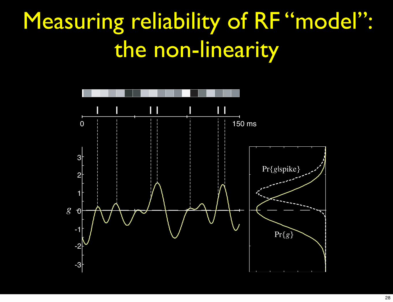
Measuring reliability of RF “model”: the non-linearity

0 150 ms

g 0

2

-2

-1

1

-3

3

Pr{g}

Pr{g|spike}

28

Generating Function g

Fir

ing R

ate

(Hz)

!0(g)

-3 -2 -1 0 1 2 30

100

200

300

"

#

Measuring reliability of RF “model”: the non-linearity

inear Kernel

Stimulus s(t)

Firing Rate!(t) K(")

Lon-linearity

#(g)Ng(t)

LN Model of Encoding

Pr{g}

Pr{g|spike}Pr{spike|g}

29

Bussgang’s Theorem

Layman’s summary:In the context of simple non-linearities, the “optimal” receptive field is STIL given by the spike-triggered average in the context of Gaussian white noise ***

30

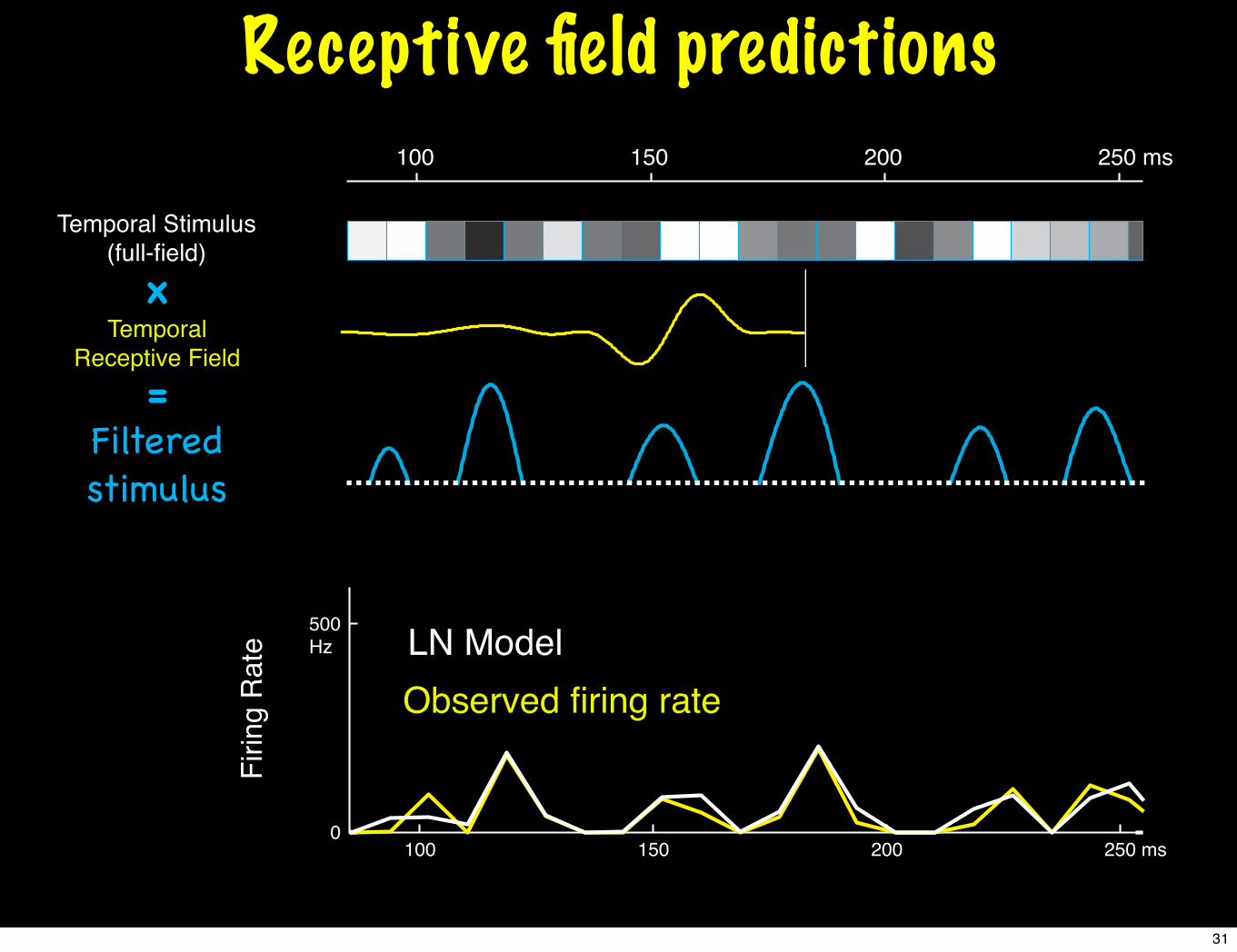
100 150 200 250 ms


Filteredstimulus

x

=Temporal

Receptive Field

Receptive field predictions

Firin

g Ra

te LN ModelObserved firing rate

100 150 200 250 ms0

500

Hz

31

How quantify quality of model fit?

Matlab Interlude

32

Problems with visual neuron modeling

3. r2 is not the best measure for evaluating a non-linear system

(also, it requires multiple repeats to estimate a good firing rate)

2. Non-linearities “force” the use of Bussgang’s theorem -> only use STA, and need noise stimuli

1. Looking at higher time resolution reveals that the LN model is insufficient

33







34

Maximum Likelihood ApproachStimulus

Response(Spike Train)

inear KernelL

on-linearityN

oisson

processP

f

k

Does data (LGN spike times) support refractory period explanation of precision?

0

500

Hz

Prob

abili

tyof

spi

ke

Likelihood: probability that model explains data

Find the “maximum likelihood”:The probability that the spikes were generated by a model with a certain choice of parameters

LL =!

tspk

log Pr{spk|tspk}!!

t

Pr{spk|t}

Firing rate when there is an observed spike

Firing rate when there is no observed spike

35

Problem: complicated function to maximize!The maximum likelihood:

LL =!

tspk

log Pr{spk|tspk}!!

t

Pr{spk|t}

Stimulus


inear KernelL

on-linearityN

oisson

processP

f

k

Paninski (2004):

No local minima in likelihood surface given certain forms of non-linearity (f)

Matlab can solve for optimal parameters in very little time!

[e.g., 2 minutes of data, 0.5 ms resolution~ 20 seconds]

36

LN model is fit “optimally” using maximum likelihood

Quick Matlab Interlude

37







38

100 150 200 250 ms


Filteredstimulus

x

=Temporal

Receptive Field

NeuronʼsFiring Rate

“LN Model”

0

500

Hz

Actual


39

Neuron's Response

"Function-based" Prediction

Spike Rasters


NeuronʼsFiring Rate

“LN Model”

0

500

Hz

Actual

40

0

500

Hz

Neuron is “tuned” to the stimulus

Need to “suppress” neuron’s response during periods of stimulus that matches RF

“Refractory”effects

30 ms

Refractoriness andNeural Precisione.g., Berry and Meister, 1998

Brillinger, 1992Keat et al., 2001Paninski, 2004

Pillow et al., 2005...

How to generate precision?

41

Generalized Linear Model (GLM)Stimulus


inear KernelL

on-linearityN

oisson

processP

f

k

Spike History

Term

+

wRP


Optimal solution for model parameters (no matter how many parameters!)

Paninski (2004):

But, spike history term does not explain the temporal resolution of the data.

42

GLM model does not explainLGN temporal precision

Data (60 reps x-validated)

LN

1.18 1.22 1.26 1.30 1.340

400

800

1200

0.5 ms resolution

Time (sec)

Fir

ing R

ate

(Hz)

GLM

Despite matchingISI distributions

0 5 10 15 20 25Interspike Interval (ms)

DataLN Model+spike history

43

0

500

HzWhat about “network” suppression?

“Tuned” Stimulus

LGN neuronspikes

Suppressionafter spikes

Others neurons in network active

Refractoriness and precision model

Network suppression model

Stimulus


RF

Spikegeneration

“Spike-Refractory

E!ects”

44

0

500

HzWhat about “network” suppression?

Refractoriness and precision model

Network suppression model

Stimulus


RF

Spikegeneration

“Spike-Refractory

E!ects”

Stimulus


RF1

Spikegeneration

RF2

(Recti!ed)Suppression

45

Directly fit *multiple* receptive fields


Stimulus


RF1

Spikegeneration

RF2


-- Alternative to spike-triggered covariance

-- Application to neurons that process stimuli

non-linearly (e.g., on-off cells in mouse retina)

-- Simplest way to incorporate two RFs

46

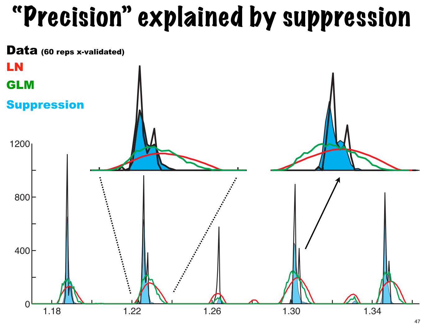
“Precision” explained by suppressionData (60 reps x-validated)

LN

1.18 1.22 1.26 1.30 1.340

400

800

1200

0.5 ms resolution

Time (sec)

Fir

ing R

ate

(Hz)

GLM

Suppression

47

2 minutes of FF stimulation

30 sec unique sequence repeated 60 times

...

Fit model to 2 min Model test

Cross-validation

0.4 0.8 1.2 1.61

2

3

Information gain (bits/spk)

Res

pons

e T

ime

Scal

e (m

s)

X cellsYcells

GLM Sup1

GLM

Sup1

X-cells(N = 13)

Y-cells(N = 10)

Info

rmat

ion

(bits

/spk

)

0.2

0.4

0.6

0.8

1.2

0.0

1.0

Significant improvement across all recorded neurons

48

Stimulus


RF1

Spikegeneration

RF2


Precision computation

0 20 40 60 80 100 120 140 160

- sup

linear

!ring rate

0 140 160

- sup

!ring rate-100 -80 -60 -40 -20 0

Linear FilterSuppressive !lter **

49

Exc: bipolar cellInh: spiking amacrine

General role of local inhibition?

Retina

++

-local inhibitoryinterneuron

long

-rang

e ex

cita

tory

pro

ject

ion

Exc: RGC inputInh: interneurons

LGNExc: LGN inputInh: interneurons

V1

50

Circuitry of the retina

Role in spatialprocessing?

Role in temporalprocessing?

OUTER PLEXIFORMLAYER

INNER PLEXIFORMLAYER

51

Conclusions/Parting Thoughts1. Visual neuron modeling

Don’t forget the LN model -- it is everywhereBasis for sensory models in neuroscience (“minimal model”)

2. Neuroscience has been (but no longer is?) stuck with standard statistics

Brought field to where it is (VERY USEFUL) but ... could not go much furtherNeuroscience-statisticians are having large impact on basic science(Emory Brown, Liam Paninski, Rob Kass, Valerie Ventura, Han Amarsingham,... )

3. Maximum likelihood modelingSystem of models that have smooth likelihood surfaceAbility to solve higher-order models with limited data

52

models of visual neuron function - cornell...

Documents