modern pid tuning and advanced control...
TRANSCRIPT

Modern Advanced Process Control Implementation and
PID Tuning Optimization inside the DCS or PLC
Janarde Leporea, Ivan Mohler
b, Constantine Tudoran
c
a PiControl Solutions LLC, Houston, TX, USA
b Zagreb University, Zagreb, Croatia
c Consultant, Houston, TX, USA
ABSTRACT
Application of closed-loop advanced control in industry has rapidly increased since the
1990s. The terms “DCS”, “PLC”, “PID”, “APC”, “Computer Control”, “Process
Optimization”, “MPC”, “Model-Based Control” etc. are ubiquitous in process control
literature. A prerequisite for APC/MPC success is a well-designed primary PID control
platform with optimized tuning. Increasing application of advanced control schemes
places higher demands on the skills and experience level of process control engineers and
technicians. This paper describes some powerful practical process control software tools
aimed at helping control engineers and technicians to design and implement control
schemes inside the DCS for improving plant control. These tools and the methodology
can help plants to maximize production rates, minimize utilities and increase the plant’s
profits.
KEYWORDS
Process control applications, APC, advanced process control, system identification, PID
tuning simulation and optimization.
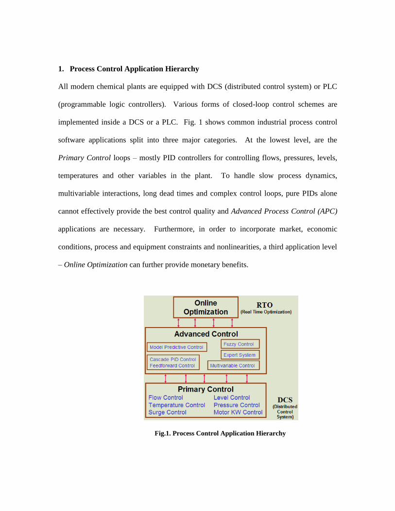
1. Process Control Application Hierarchy
All modern chemical plants are equipped with DCS (distributed control system) or PLC
(programmable logic controllers). Various forms of closed-loop control schemes are
implemented inside a DCS or a PLC. Fig. 1 shows common industrial process control
software applications split into three major categories. At the lowest level, are the
Primary Control loops – mostly PID controllers for controlling flows, pressures, levels,
temperatures and other variables in the plant. To handle slow process dynamics,
multivariable interactions, long dead times and complex control loops, pure PIDs alone
cannot effectively provide the best control quality and Advanced Process Control (APC)
applications are necessary. Furthermore, in order to incorporate market, economic
conditions, process and equipment constraints and nonlinearities, a third application level
– Online Optimization can further provide monetary benefits.
Fig.1. Process Control Application Hierarchy

Primary control and DCS-based Advanced Control, if correctly implemented can
significantly increase the plant’s profit margins. Optimized primary and advanced
control stabilizes process operation and pushes the operation closer to process, equipment
and economic constraints. This increases production rates, minimizes operating costs and
improves product quality.
2. Challenges facing Modern Control Rooms
The increasing use of primary and advanced control poses the following challenges in the
control rooms:
1. New control engineers and DCS/PLC technicians come into the plant on regular
basis. They need to be trained on practical process control.
2. Many primary and DCS-based advanced control concepts cannot be taught easily
at schools and colleges. Learning practical process control skills quickly is not
easy.
3. Changes in process or operating conditions, nonlinearities, external unmeasured
disturbances can impact closed-loop control quality resulting in inefficient
operation including lost production and could even cause equipment shutdowns
and safety/reliability incidents.
4. Constant software and hardware upgrades add to the maintenance challenges in
the control room.

3. Attractive Opportunities to Increase Profits using DCS Advanced Control
Using modern DCS and PLCs, various powerful, robust money-making control schemes
can be implemented. This paper describes several powerful techniques for designing and
implementing DCS/PLC-resident advanced control schemes. These include:
1. Process Dynamics Identification
2. Primary and Advanced Control PID Tuning Optimization
3. Online Adaptive Control
4. Model-Based Control for Product Quality
5. Production Rate Maximization
6. Engineer, Technician and Operator Practical Process Control Training
4. Process Control Tools for Control Rooms
Any modern DCS or PLC is capable of archiving real-time process data that can be
exported in Excel files for data analysis. Many DCS and PLC systems also have OPC
servers and OPC client software that allows trending and archiving of real-time process
data. Process data analysis can help to identify system dynamics, which in turn can be
used for optimizing base-level primary PID controllers and also for designing APC
systems. In this paper, we describe some powerful tools and methods designed especially
for use by control engineers and technicians in the plant control room environment.
These tools are simple and can be used effectively by both engineers and technicians.
Various illustrative examples on the application of these tools in the chemical plant
control rooms are described below.

5. Process Dynamics Identification
Chemical processes range process dynamics from as fast as milliseconds on compressor
surge control and motor control to as low as many hours in tall super-fractionators
distillation columns. In modern control rooms, there are plenty of data sets available
containing the controller OP (output), PV (process variable) and SP (set point). Data may
contain OP step changes with the controller in manual mode, or may contain SP changes
in auto mode. There are many opportunities in the plant where the operator may have
made changes to the SP or OP. All these data sets are abundantly available from the
plants data historians that continuously archive the data.
With modern process dynamics identification software tools like Pitops, the identification
takes just a few minutes. See Fig. 2 showing pressure control (PC) data.
Fig.2. Pressure Control Transfer Function Dynamics Identification
Transfer Function
Model Prediction
Reactor
Pressure (CV)
Control Valve
Step Changes
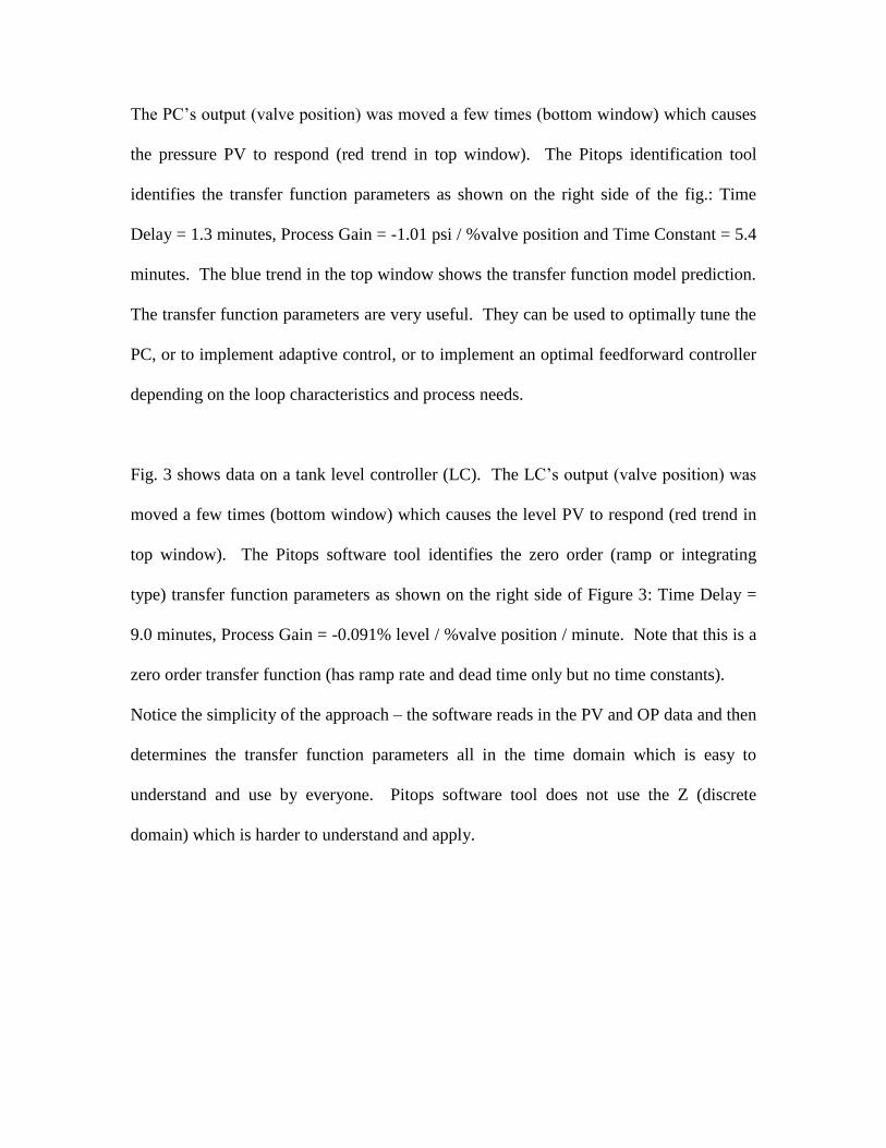
The PC’s output (valve position) was moved a few times (bottom window) which causes
the pressure PV to respond (red trend in top window). The Pitops identification tool
identifies the transfer function parameters as shown on the right side of the fig.: Time
Delay = 1.3 minutes, Process Gain = -1.01 psi / %valve position and Time Constant = 5.4
minutes. The blue trend in the top window shows the transfer function model prediction.
The transfer function parameters are very useful. They can be used to optimally tune the
PC, or to implement adaptive control, or to implement an optimal feedforward controller
depending on the loop characteristics and process needs.
Fig. 3 shows data on a tank level controller (LC). The LC’s output (valve position) was
moved a few times (bottom window) which causes the level PV to respond (red trend in
top window). The Pitops software tool identifies the zero order (ramp or integrating
type) transfer function parameters as shown on the right side of Figure 3: Time Delay =
9.0 minutes, Process Gain = -0.091% level / %valve position / minute. Note that this is a
zero order transfer function (has ramp rate and dead time only but no time constants).
Notice the simplicity of the approach – the software reads in the PV and OP data and then
determines the transfer function parameters all in the time domain which is easy to
understand and use by everyone. Pitops software tool does not use the Z (discrete
domain) which is harder to understand and apply.

Fig.3. Level Control Transfer Function Dynamics Identification
Fig. 4 shows more step test data on the same level control example. With more step tests
on this control loop, some nonlinearity is visible; this can be because of valve stiction,
flow meter problems or unmeasured disturbances that could mask the effect of the control
valve step tests. The Pitops software identification algorithm determines control valve
stiction also based on the OP and PV data.
Fig.4. Level Control Transfer Function Dynamics Identification – Multiple Step
Tank Level
(CV)
Transfer Function
Model Prediction
Tank Flow Outlet
Valve Position
Tank Level
(CV)
Transfer Function
Model Prediction
Tank Flow Outlet
Valve Position
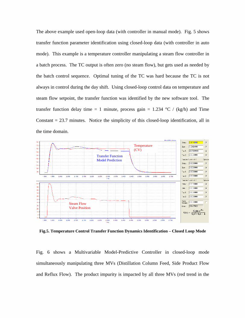
The above example used open-loop data (with controller in manual mode). Fig. 5 shows
transfer function parameter identification using closed-loop data (with controller in auto
mode). This example is a temperature controller manipulating a steam flow controller in
a batch process. The TC output is often zero (no steam flow), but gets used as needed by
the batch control sequence. Optimal tuning of the TC was hard because the TC is not
always in control during the day shift. Using closed-loop control data on temperature and
steam flow setpoint, the transfer function was identified by the new software tool. The
transfer function delay time = 1 minute, process gain = 1.234 °C / (kg/h) and Time
Constant = 23.7 minutes. Notice the simplicity of this closed-loop identification, all in
the time domain.
Fig.5. Temperature Control Transfer Function Dynamics Identification – Closed Loop Mode
Fig. 6 shows a Multivariable Model-Predictive Controller in closed-loop mode
simultaneously manipulating three MVs (Distillation Column Feed, Side Product Flow
and Reflux Flow). The product impurity is impacted by all three MVs (red trend in the
Temperature
(CV)
Transfer Function
Model Prediction
Steam Flow
Valve Position

top trend). The software identifies all three second order transfer functions with dead
time simultaneously using the closed-loop data.
This identification can be used to improve the step response coefficient models or
transfer function models used in any of the commercially used multivariable model-
predictive controllers to improve the controller performance.
Fig.6. Multivariable Distillation Transfer Function Dynamics Identification – Closed Loop Mode
6. PID Tuning Optimization
Knowing the process transfer function helps to optimally tune base-level and
cascade/advanced control type PIDs. Fig. 7 shows an industrial pressure control
example. The bottom window shows the PC’s output. The top window shows the SP
(blue trend) and PV (red trend).
MV1- Feed
MV2- Side Product
MV3- Reflux
Product Impurity Transfer Function Model

The PC’s objective is to not only provide crisp SP control but also to respond
aggressively when hit by a disturbance. Disturbances can come and go anytime and it is
important for the PC to respond quickly by closing or opening the valve immediately.
The key is that such aggressive control action needed during disturbance rejection should
not result in sustained oscillations at steady state.
The tuning optimization software generates such tuning parameters that give crisp, non-
oscillatory SP control while responding quickly during fast and large disturbances. Use
of the tuning software on this example resulted in increasing the controller proportional
gain from 2 to 11 in one step and the integral from 8 to 3 minutes.
Without modern optimization software tools, control engineers confronted with tuning
such a PC would not have the confidence to increase the controller gain that drastically
from 2 to 11 in one step. They would have crept up the gain from 2 to 2.5 and 3 etc. over
a much longer time period. And since the disturbance does not come all the time, it is
hard to manually tune the loop for optimal control without the help of modern software
tools.

Fig.7. PID Tuning Optimization in presence of SP change and typical disturbance
Fig. 8 shows how the software optimizes PID tuning in the presence of signal noise. It
mimics the real process by simulating the same level and frequency of white signal noise
seen in the real process. In just a few minutes, the optimizer converts the real process
signal characteristics into a custom simulation comprising typical set point changes,
signal noise and disturbances followed by PID tuning optimization.
Pressure
(PV)
Pressure Control
Setpoint
PID Output
(Control Valve)
Disturbance
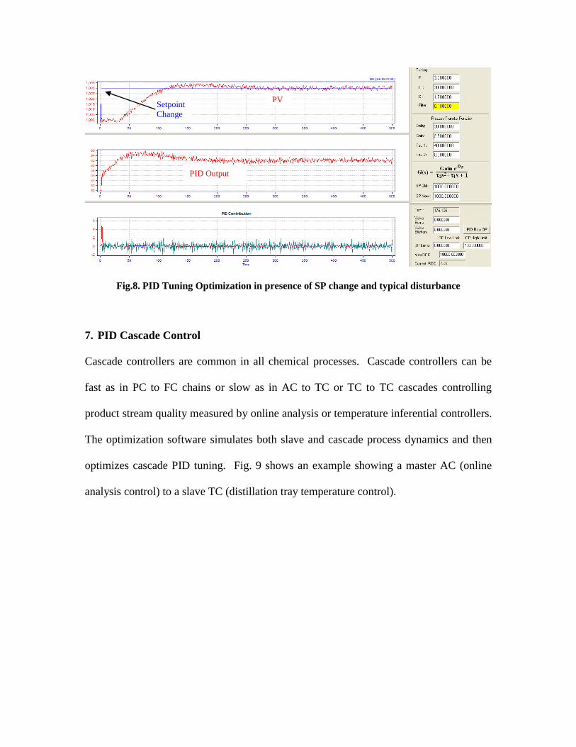
Fig.8. PID Tuning Optimization in presence of SP change and typical disturbance
7. PID Cascade Control
Cascade controllers are common in all chemical processes. Cascade controllers can be
fast as in PC to FC chains or slow as in AC to TC or TC to TC cascades controlling
product stream quality measured by online analysis or temperature inferential controllers.
The optimization software simulates both slave and cascade process dynamics and then
optimizes cascade PID tuning. Fig. 9 shows an example showing a master AC (online
analysis control) to a slave TC (distillation tray temperature control).
PV Setpoint
Change
PID Output
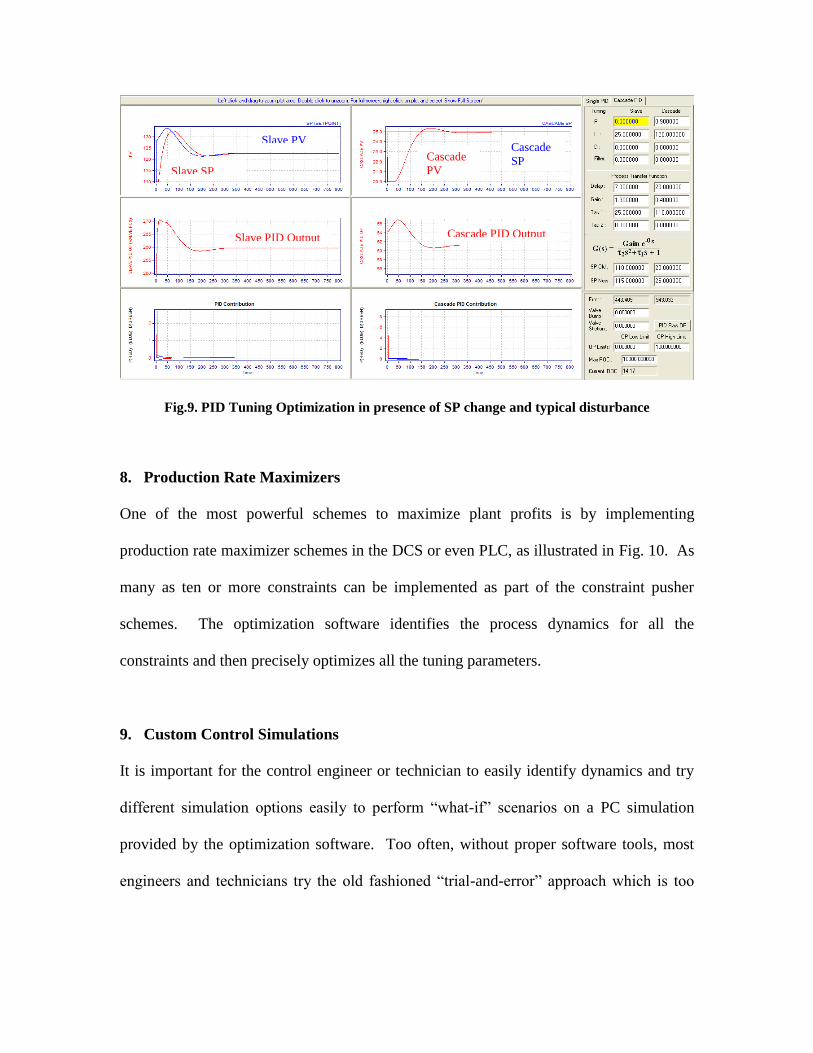
Fig.9. PID Tuning Optimization in presence of SP change and typical disturbance
8. Production Rate Maximizers
One of the most powerful schemes to maximize plant profits is by implementing
production rate maximizer schemes in the DCS or even PLC, as illustrated in Fig. 10. As
many as ten or more constraints can be implemented as part of the constraint pusher
schemes. The optimization software identifies the process dynamics for all the
constraints and then precisely optimizes all the tuning parameters.
9. Custom Control Simulations
It is important for the control engineer or technician to easily identify dynamics and try
different simulation options easily to perform “what-if” scenarios on a PC simulation
provided by the optimization software. Too often, without proper software tools, most
engineers and technicians try the old fashioned “trial-and-error” approach which is too
Cascade
PV
Slave PV
Slave PID Output
Cascade
SP Slave SP
Cascade PID Output

slow and ineffective. Fig. 11 shows how a sinusoidal disturbance can be quickly added
to a simulation to check the impact of tuning changes and controller output response.
10. Feedforward Control
In all chemical processes, control quality can be significantly improved on various
important control schemes using feedforward control. Unfortunately, almost all
feedforward tuning parameters are estimated today in the control room by trial-and-error
or “best-guessed” estimates.
The software tool provides powerful functionality to mathematically identify the
feedforward parameters - lead, lag, gain and dead time. Understanding how feedforwards
work allows building creative new applications all inside in the DCS or PLC for
numerous other innovative purposes.
Fig.10. Production Rate Maximizer Controllers inside DCS or PLC

Fig.11. Adding a Sinusoidal Disturbance to a Setpoint Change
Fig. 12 shows a pulse signal input to a feedforward transfer function with the lead
constant less than the lag constant.
Fig.12. Higher Lag Constant in a Feedforward Scheme
Fig. 13 shows a pulse signal input to a feedforward transfer function with the lead
constant higher than the lag constant. Notice the differences in the response in the two
cases.
Simulated Sinusoidal Disturbance
Setpoint Change
PID Output
Lead Constant Less than
Lag Constant

Fig.13. Higher Lead Constant in a Feedforward Scheme
All these simulations can calculations can be easily performed with the software tool. By
mastering the quantitative details of how feedforwards work, an engineer or technician
can easily build powerful feedforward control schemes inside the DCS or PLC with
numerous benefits. Fig. 14 shows a sample calculation overview of a feedforward
control scheme.
Fig.14. Feed forward Parameter Calculations
Lead Constant More
than Lag Constant

11. Model-Based Controllers
Another big opportunity is the implementation of model-based controllers in the DCS or
PLC. Any model based on rigorous, empirical, semi-empirical or regressed models can
be implemented in the DCS using once through or iterative calculations. Such models
can be used to implement closed-loop controllers in the DCS or PLC. Furthermore,
measurement feedback such as from online gas chromatographs or laboratory analysis
can be incorporated into the predictive models. The modern software tools help to design
model-based controllers with predictive, corrective and feedback closed-loop control
action. An overview of the implementation is shown in Fig. 15.
Fig.15. Implementing Model-Based Control inside DCS or PLC

Fig.16. Process Control Simulation Functions
12. Summary
Since the 80s, an increasingly large number of DCS and PLC systems are controlling
chemical processes. For many years, the basic hardware and software skills were being
learnt and mastered to ensure control system reliability and safety. Now, the control
community is past that stage and is ready to push the functions and capabilities of the
DCS and PLC systems like never before. Numerous powerful process control
applications can be implemented in the DCS or PLC with increased recurring average
annual profits ranging from $50K to $3 million, depending on the size and type of the
plant. However, to realize these benefits, chemical plant managements need to properly
train their control engineers and technicians and provide modern process control software
tools to aid their implementation and design.
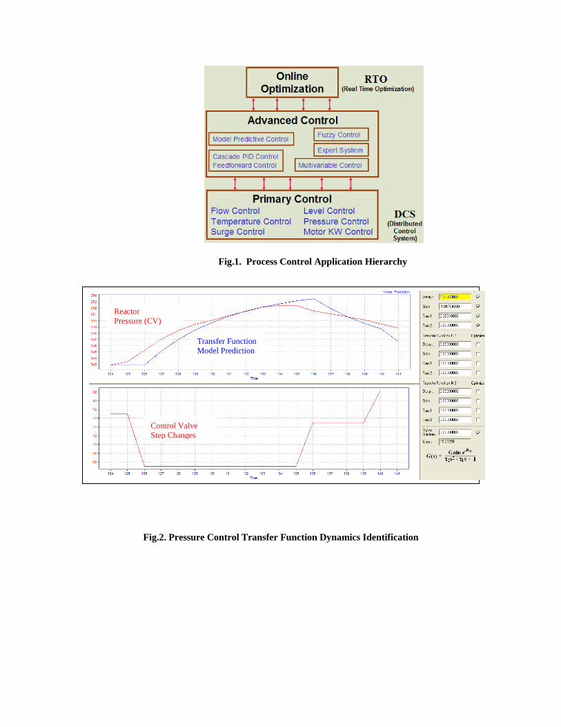
Fig.1. Process Control Application Hierarchy
Fig.2. Pressure Control Transfer Function Dynamics Identification
Transfer Function
Model Prediction
Reactor
Pressure (CV)
Control Valve
Step Changes

Fig.3. Level Control Transfer Function Dynamics Identification
Fig.4. Level Control Transfer Function Dynamics Identification – Multiple Step
Tank Level
(CV)
Transfer Function
Model Prediction
Tank Flow Outlet
Valve Position
Tank Level
(CV)
Transfer Function
Model Prediction
Tank Flow Outlet
Valve Position
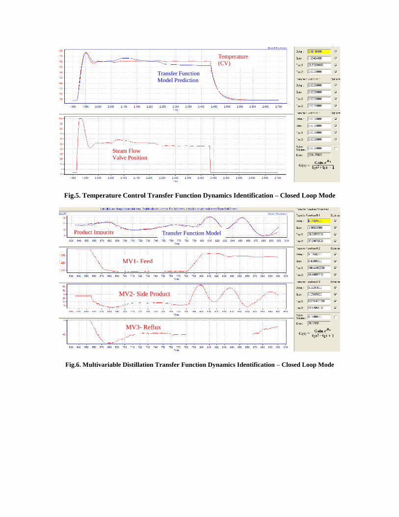
Fig.5. Temperature Control Transfer Function Dynamics Identification – Closed Loop Mode
Fig.6. Multivariable Distillation Transfer Function Dynamics Identification – Closed Loop Mode
MV1- Feed
MV2- Side Product
MV3- Reflux
Product Impurity Transfer Function Model
Temperature
(CV)
Transfer Function
Model Prediction
Steam Flow
Valve Position

Fig.7. PID Tuning Optimization in presence of SP change and typical disturbance
Fig.8. PID Tuning Optimization in presence of SP change and typical disturbance
PV Setpoint
Change
PID Output
Pressure
(PV)
Pressure Control
Setpoint
PID Output
(Control Valve)
Disturbance

Fig.9. PID Tuning Optimization in presence of SP change and typical disturbance
Fig.10. Production Rate Maximizer Controllers inside DCS or PLC
Cascade
PV
Slave PV
Slave PID Output
Cascade
SP Slave SP
Cascade PID Output
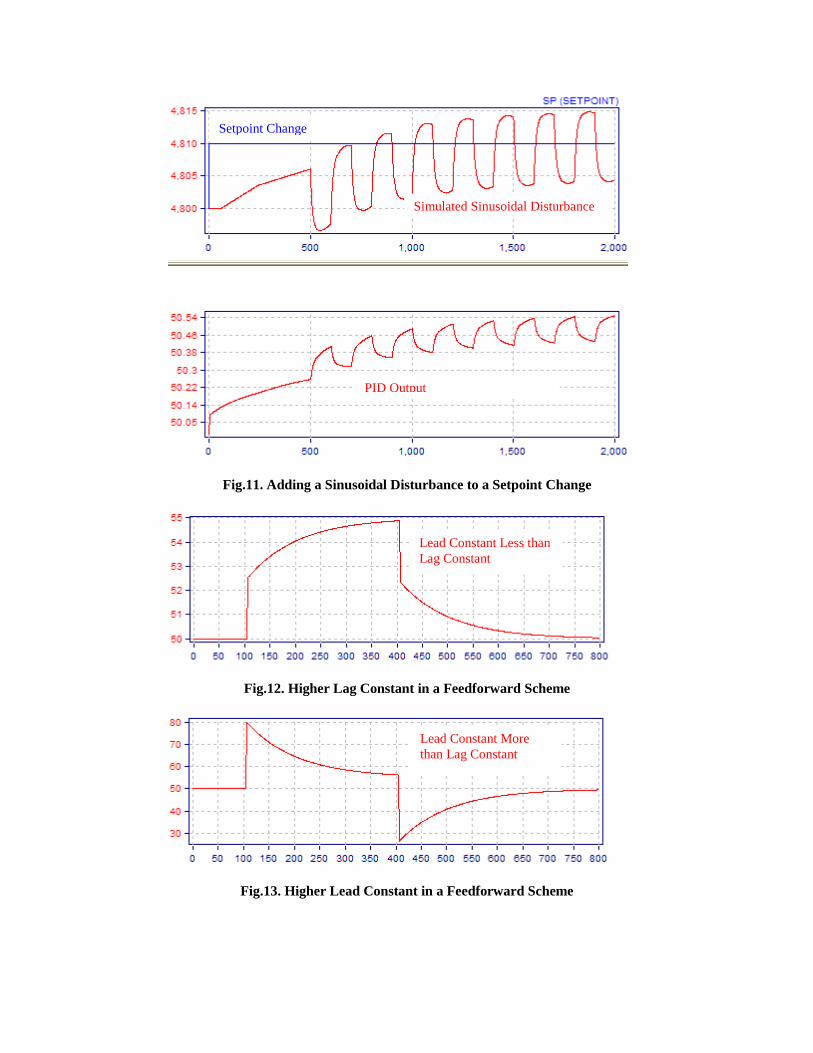
Fig.11. Adding a Sinusoidal Disturbance to a Setpoint Change
Fig.12. Higher Lag Constant in a Feedforward Scheme
Fig.13. Higher Lead Constant in a Feedforward Scheme
Lead Constant More
than Lag Constant
Lead Constant Less than
Lag Constant
Simulated Sinusoidal Disturbance
Setpoint Change
PID Output

Fig.14. Feed forward Parameter Calculations
Fig.15. Implementing Model-Based Control inside DCS or PLC
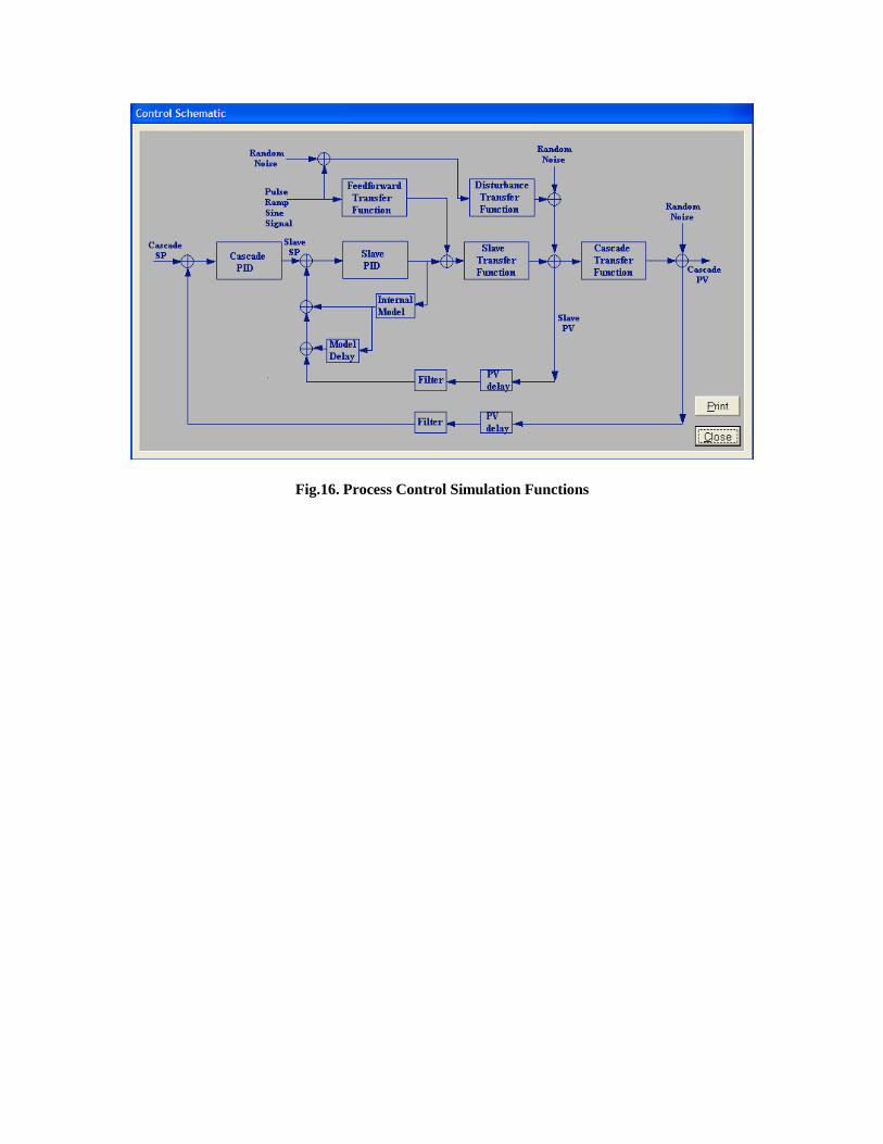
Fig.16. Process Control Simulation Functions