Mark Grigoleit

Principal Simulation Consultant

Optika Solutions Pty Ltd

Contents Introduction to iron ore

Part 1 – the problem

Part 2 – the solution

Part 3 – the results

Part 1: The problem Fun facts about Fe:

4th most common element in earth’s crust (about 5%) after Oxygen, Silicon and Aluminum

Has been mined for about 5,000 years

Exists mostly as oxides

Hematite (Fe2O3) and Magnetite (Fe3O4)

Refined back into metal by removing the oxygen in a furnace

Whyalla mines in SA

Infrastructure Diggers

Crushers and screening

Rail transport to shed

Ship loading by barge

All these activities have variability

No closed form solution

This is the motivation for using simulation modelling

Grade Variability Mine blocks have only estimates of grade from drill

cores

Mine plan is order of digging

After crushing, an assay to determine actual grades

What tonnes and grade will ultimately be exported – this is the devil in the problem

The economic facts Cost of production is $35 to $75 per tonne, depending

on the operation

High grade is considered to be ~63% Fe (or 90% hematite, rest is silica, alumina)

Lower grade material can be beneficiated (OBP) at extra cost (wash the sand off)

Grade penalties apply for deviation from agreed grade

Shipping delays may incur demurrage charges

The Problem To work out in advance what ore can be produced

Time frame of one year or more

How many tonnes of ore

And at what grade

Part 2: The solution We employ a discrete event model that uses built-in

distributions to account for local variability – processing rates, travel times, down times, weather delays, etc.

The model consists of many objects, with each piece of equipment represented as an object

The model has over 1,000 input variables

The model Model built in a simulation language called SLX

Operates on daily plan

Plan created by LP formulation of problem

Model took 4 smart guys 1 year to construct

Optimisation Problem Goal of the optimisation – supply export tonnes

(169,000) within grade limits

Types of constraints – time, tonnes, grade

Three ship lookahead (one month)

Local optimisation for building feed piles

Global optimisation for building ship consignments

Implemented with AIMMS

Multi-level grade control LP optimisation to select ore

Local level: ROM piles – crusher – stockpiles

Local level: stockpiles – rail – shed

Local level: shed + rail direct load to ship

Global level: from mine blocks to ship

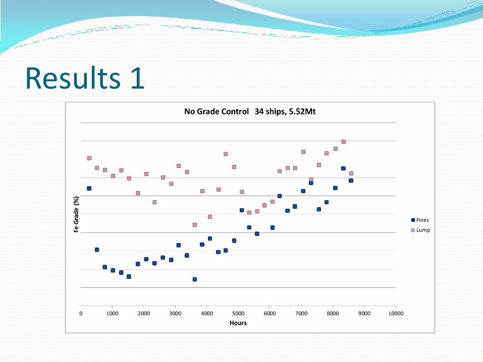
Results 1

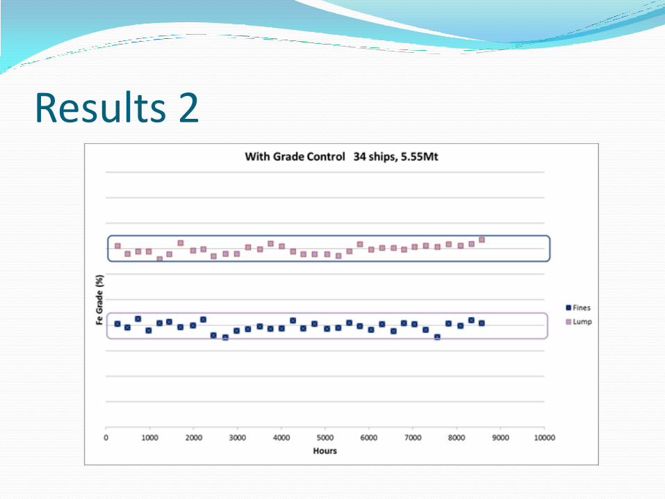
Results 2

Review Daily plan by LP solve takes seconds

Variability of shipped ore grade minimised

No loss of total exported tonnes

Detailed modelling allows prediction of tonnes and grade given changes in actual ore body or external market conditions

Conclusion For very large and complex operations, sometimes the

only way to evaluate performance is to use a simulation model.

In the case of grade variability of iron ore, this has proven successful.