modular forms and elliptic curves - lmu
TRANSCRIPT

Joachim Wehler
Modular Formsand Elliptic Curves
DRAFT, Release 1.50
April 16, 2021

2
c© Joachim Wehler, 2020, 2021
I prepared these notes for the participants of the lectures. The lecture took place atthe mathematical department of LMU (Ludwig-Maximilians-Universitat) atMunich. The first time during the winter term 2017/18 and then during the winterterm 2020/21. Some parts of the notes rely on notes of an unpublished lectureof O. Forster.
Compared to the oral lecture in class these written notes contain some additionalmaterial.
I thank all participants - in particular W. Hensgen - for pointing out some errorsand for their proposals for improvement. Please report to
any further errors or typos, adding the version of the lecture notes.
Release notes:
• Release 1.50: Update acknowledgment.• Release 1.49: Chapter 5. Remark 5.15 moved from Chapter 7. Chapter 7.
Revision.• Release 1.48: Chapter 6. Revision, Lemma 6.21 added.• Release 1.47: Chapter 5. Proposition 5.9 added.• Release 1.46: Chapter 3 and Chapter 2. Revision.• Release 1.45: Chapter 4. Revision.• Release 1.44: Chapter 5. Revision.• Release 1.43: Chapter 5. Theorem 5.25 proof corrected.• Release 1.42: Chapter 5. Theorem 5.25 corrected. Chapter 6 minor revisions.• Release 1.41: Chapter 7. Section 7.2 added. Chapter 5. Theorem 5.23 expanded.
Theorem 5.25 expanded and corollary integrated.• Release 1.40: Chapter 7. Section 7.1 added.• Release 1.39: Chapter 4. Proposition 4.25 expanded.• Release 1.38: Chapter 6. Sections 6.1 and 6.2 added.• Release 1.37: Chapter 5. Section 5.2, Lemma 5.24 replaced by new version,
subsequent Corollary added, Theorem 5.25 adapted, renumbering, Section 5.3added.
• Release 1.36: Chapter 5. Section 5.2, Proposition 5.28 added, minor revision.• Release 1.35: Chapter 5. Section 5.2 added.• Release 1.34: Chapter 5. Section 5.1, minor revision.• Release 1.33: Chapter 4. Example 4.39 expanded.• Release 1.32: Chapter 5. Section 5.1 added.• Release 1.31: Chapter 4. Section 4.2, Definition 4.19 expanded, Lemma 4.30
and Theorem 4.31 clarified, Remark 4.27 added, renumbering, minor revision.Section 4.3 added.

3
• Release 1.30: Chapter 4. Section 4.2, Example 4.36 added, minor revision.• Release 1.29: Chapter 3, Lemma 3.4, exponent of determinant changed.
Chapter 4, Example 4.4 added. Renumbering, Section 4.2 added.• Release 1.28: Chapter 4. Proposition 4.8, proof corrected. Section 4.1, minor
revisions.• Release 1.27: Chapter 2, Remark 2.30, formulas corrected by extended
Legendre symbol and Kronecker symbol. Chapter 4, Proposition 4.6 added,minor revisions, renumbering. List of results updated.
• Release 1.26: Chapter 3, proof of Lemma 3.4: formula corrected. Chapter 4,minor revisions
• Release 1.25: Chapter 4, Section 4.1 added.• Release 1.24: Minor revisions.• Release 1.23: Minor revisions.• Release 1.22: Chapter 3 completed.• Release 1.21: Section 3.2, some typos corrected.• Release 1.20: Minor revisions.• Release 1.19: Minor revisions.• Release 1.18: Chapter 2, Remark 3.5 added.• Release 1.17: Minor revisions.• Release 1.16: Chapter 2, Remark 2.8, Example 2.11, Lemma 2.26 corrected.
Chapter 3, Section 3.1 reordered.• Release 1.15: Chapter 3, Remark 3.7 added, Remark 3.7 expanded, minor
revisions, renumbering.• Release 1.14: Minor revisions.• Release 1.13: Chapter 3, Section 3.2 added. List of results added.• Release 1.12: Chapter 1, Proposition 1.19 added, renumbering. Chapter 2,
Remark 2.17 added, renumbering. Chapter 3, Section 3.1 added.• Release 1.11: Chapter 2 completed.• Release 1.10: Chapter 2, Section 2.2 correction of some typos.• Release 1.9: Chapter 1, revision of Corollary 1.9 and 1.10, Lemma 1.13,
Corollary 1.15 and Theorem 1.21. Further minor revisions.• Release 1.8: Chapter 2 minor revision.• Release 1.7: Chapter 2 minor revision, some additions.• Release 1.6: Chapter 2 minor revision.• Release 1.5: Chapter 2, Sections 2.1 and 2.2 added.• Release 1.4: Chapter 1, minor revision.• Release 1.3: Introduction added.• Release 1.2: Chapter 1, minor revision.• Release 1.1: Complete revision, starting with Chapter 1.


Contents
Introduction . . . . . . . . . . . . . . . . . . . . . . . . . . . . . . . . . . . . . . . . . . . . . . . . . . . . . . . 1
PARI files . . . . . . . . . . . . . . . . . . . . . . . . . . . . . . . . . . . . . . . . . . . . . . . . . . . . . . . . . 3
Part I General Theory
1 Elliptic functions . . . . . . . . . . . . . . . . . . . . . . . . . . . . . . . . . . . . . . . . . . . . . . . 91.1 The field of elliptic functions . . . . . . . . . . . . . . . . . . . . . . . . . . . . . . . . . 91.2 The Weierstrass ℘-function . . . . . . . . . . . . . . . . . . . . . . . . . . . . . . . . . . 141.3 Abel’s theorem. . . . . . . . . . . . . . . . . . . . . . . . . . . . . . . . . . . . . . . . . . . . . 24
2 The modular group Γ and its Hecke congruence subgroups Γ0(N) . . . 312.1 The moduli space of complex tori and group actions . . . . . . . . . . . . . 312.2 Topology of the orbit space of the Γ -action . . . . . . . . . . . . . . . . . . . . . 462.3 Modular curves X(Γ0(N)) as compact Riemann surfaces . . . . . . . . . . 63
3 The algebra of modular forms . . . . . . . . . . . . . . . . . . . . . . . . . . . . . . . . . . . 813.1 Modular forms and cusp forms . . . . . . . . . . . . . . . . . . . . . . . . . . . . . . . 813.2 Eisenstein series and the algebra of modular forms of Γ . . . . . . . . . . 903.3 Generalization to Hecke congruence subgroups Γ0(N) . . . . . . . . . . . . 117
4 Elliptic curves . . . . . . . . . . . . . . . . . . . . . . . . . . . . . . . . . . . . . . . . . . . . . . . . . 1254.1 Embedding tori as plane cubic hypersurfaces . . . . . . . . . . . . . . . . . . . 1254.2 Elliptic curves over subfields of C . . . . . . . . . . . . . . . . . . . . . . . . . . . . . 1394.3 Elliptic curves over finite fields . . . . . . . . . . . . . . . . . . . . . . . . . . . . . . . 169
5 Introduction to Hecke theory and applications . . . . . . . . . . . . . . . . . . . . 1815.1 Hecke operators of the modular group and their eigenforms . . . . . . . 1815.2 The Petersson scalar product . . . . . . . . . . . . . . . . . . . . . . . . . . . . . . . . . 2005.3 Numerology: Lagrange, Jacobi, Ramanujan, Mordell . . . . . . . . . . . . . 217
Part II Advanced Theory
v

vi Contents
6 Application to imaginary quadratic fields . . . . . . . . . . . . . . . . . . . . . . . . . 2296.1 Imaginary quadratic fields and tori with complex multiplication . . . . 2296.2 Modular polynomials . . . . . . . . . . . . . . . . . . . . . . . . . . . . . . . . . . . . . . . 2366.3 Fractional ideals and the class number formula . . . . . . . . . . . . . . . . . . 251
7 Outlook: Modular elliptic curves, monstrous moonshine . . . . . . . . . . . . 2617.1 Modular elliptic curves . . . . . . . . . . . . . . . . . . . . . . . . . . . . . . . . . . . . . . 2617.2 Monstrous moonshine . . . . . . . . . . . . . . . . . . . . . . . . . . . . . . . . . . . . . . . 266
List of results and some outlooks . . . . . . . . . . . . . . . . . . . . . . . . . . . . . . . . . . . . . 273
References . . . . . . . . . . . . . . . . . . . . . . . . . . . . . . . . . . . . . . . . . . . . . . . . . . . . . . . . . 277
Index . . . . . . . . . . . . . . . . . . . . . . . . . . . . . . . . . . . . . . . . . . . . . . . . . . . . . . . . . . . . . 281

Introduction
Modular Forms and elliptic curves are a classical domain from mathematics. Atleast, since the proof of Fermat’s last conjecture the domain attracts widespread at-tention. The domain of Modular Forms integrates the three mathematical disciplinesComplex Analysis, Algebraic Geometry, and Algebraic Number Theory.
Elliptic curves can be investigated by different mathematical methods.
• Algebraic geometry: Elliptic curves are the zero-sets of polynomials.
• Complex analytic geometry: When considered as Riemann surfaces then ellipticcurves are complex tori.
• Arithmetic geometry: Elliptic curves can be defined over different fields, e.g.over Q or Fp and over the ring Z.
The algebraic point of view identifies complex elliptic curves with smooth cubichypersurfaces of P2. Hence elliptic curves are the first ones in the series of cubichypersurfaces in complex projective space Pn, n≥ 2. The higher dimensionalcubics are also challenging examples, see [29, Chap.V, §4], [31].
Chapter 1 introduces elliptic functions as doubly periodic, meromorphic func-tions in the complex plane C. The period group is a lattice Λ ⊂ C. The main tool tostudy elliptic function is the residue theorem.
Chapter 2 characterizes elliptic functions as meromorphic functions on thetorus C/Λ . The classes of biholomorphically equivalent complex tori are the orbitsof a group action of the modular group
Γ ×H−→H
The quotients
1

2 Introduction
Γ0(N) \H
of the restricted action of the Hecke congruence subgroups
Γ0(N)⊂ Γ
are Riemann surfaces with compactifications X0(N).
Chapter 3 introduces modular forms and cusp forms as holomorphic functionson H∪∞with a certain transformation behaviour with respect to the Γ0(N)-action.These functions unreveal themselves as meromorphic differential forms on the mod-ular curve X0(N). The Riemann-Roch theorem computes the dimensions of the vec-tor spaces of modular forms and cusp forms.
Chapter 4 makes a new start from the viewpoint of algebraic geometry: Complextori embed as elliptic curves into the complex projective plane. They can be repre-sented as non-singular cubic curves, defined as zero set of a Weierstrass polynomial.The main tool to represent a complex torus as an elliptic curve is the Weierstrass ℘-function and its differential equation. Conversely, each complex elliptic curve arisesas embedding of a complex torus.
Choosing different fields for the coefficents of the Weierstrass polynomials al-lows to consider elliptic curves defined over C,Q,Z or even over the finite fields Fp.The focus of the chapter are some relations between complex analytic geometry, al-gebraic geometry and arithmetic geometry.
Chapter 5 considers families of Hecke operators, which are linear endomor-phisms on the finite dimensional vector spaces of modular forms. Each family ofHecke operators acts on a given vector space of modular forms of fixed weight. Onthe corresponding subspace of cusp forms the family can be diagonalized simulta-neously, a result which relies on the Petersson scalar product. As an application thechapter proves some theorems from algebraic number theory related to Lagrange,Jacobi, Ramanujan, Mordell and other mathematicians.
In the second, more advanced part of the lecture notes Chapter 6 deals withdeeper applications of the theory of modular forms to algebraic number theory. Thechapter investigates the relation between tori with complex multiplication and imag-inary quadratic number fields. The main role is played by the modular invariant j.As an application the chapter proves a lower bound of the class number.
The final Chapter 7 gives an outlook to the modularity theorem for elliptic curves,which plays the dominant role in Wiles’ proof of the Fermat conjecture. A secondsection gives an outlook to the moonshine relation between the Fourier coefficientsof the modular j-invariant and the dimensions of the irreducible representations ofthe monster group, which at day culminates in the work of Borcherds.
It is also the aim of these lecture notes to illustrate their results and the outlookby a series of numerical calculations using a computer algebra system.

PARI files
Chapter 1:
• Weierstrass_p_function_08: Laurent expansion of theWeierstrass ℘-function and its derivative, cf. Remark 1.14.
Chapter 2
• modular_curve_as_covering: Genus, degree and further parameters ofmodular curve X0(N), cf. Remark 2.30.
Chapter 3
• Congruence_subgroup_19: Dimension of Mk(Γ0(pn)) via Riemann-Roch,cf. Remark 3.27.
Chapter 4
• Torus_to_Weierstrass_equation_01: The plane cubic of anembedded torus, cf. Example 4.4
• Elliptic_curve_plot_06: Plot of some plane cubics, cf. Example 4.29.
• Elliptic_curve_02: Invariants of some plane cubics, cf. Example 4.29.
• Elliptic_curve_weierstrass_equation_12: Global minimalWeierstrass polynomial and its discriminant, cf. Example 4.39.
• Elliptic_curve_Hasse_estimate_05: Hasse estimate for numberof Fp-rational points, cf. Remark 4.42.
• Elliptic_curve_04_02: Analytic rank of elliptic curves, cf. Remark 4.47.
3

4 PARI files
Chapter 5
• Hecke_matrix_02: Hecke operator T2 ∈ End(S28(Γ )), cf. Example 5.14.
• Congruence_subgroup_20: Oldforms and newforms for different Γ0(N),cf. Example 5.30.
• Modular_forms_theta_01: 4-squares theorem and similardecompositions, cf. Example 5.39.
Chapter 6
• modular_polynomial_01: Modular polynomials of different levels, cf.Example 6.9.
• modular_polynomial_02: The polynomials Φm and their factorization, cf.Example 6.11.
Chapter 7
• Elliptic_curve_taniyama_10: Illustration of Wiles’ theorem by somenumerical examples, cf. Example 7.7.
The PARI-files of these lecture notes are contained in a separate folder. It isrecommended to download all of them together, because some of them will callother files. After downloading the PARI files into the working directory of PARI agiven file can be called by the command
\r filename
For more information see the PARI manual from the PARI homepage.

Part IGeneral Theory

6
The context of Chapter 1 is complex analysis on domains in the complex plane.The base field is the field C of complex numbers. We develop the theory of ellipticfunctions, i.e. doubly periodic meromorphic functions. Classical tools are Laurentseries and the residue theorem for meromorphic functions. The period group ofdoubly periodic functions are lattices in C.
The view point of Chapter 2 are compact Riemann surfaces. We continue work-ing with the base field C, but now the domain is a complex manifold. The mostsimple example of a compact Riemann surface is the Riemann sphere P1(C). Mero-morphic functions are holomorphic maps into the Riemann sphere. A second classof compact Riemann surfaces are complex tori. The doubly periodic meromorphicfunctions from Chapter 1 are meromorphic functions on a complex torus. The maintools from the theory of Riemann surfaces are line bundles, divisors and the Theo-rem of Riemann-Roch. The set of isomorphy classes of complex tori turns out to bethe orbit space of the modular group SL(2,Z) acting on the upper half plane H. Weshow that the compactified orbit space is biholomorphic equivalent to P1(C).
Chapter 4 switches from the analytic theory to an algebraic context. We con-sider the Riemann sphere from an algebraic point of view and study non-singularcurves C in the projective space P1(C), now equipped with the Zariski topology.These curves are the zero set of one or more homogeneous polynomials. The small-est subfield k ⊂ C which comprises their coefficients is the field of definition of C.As a consequence we extend the range of base fields under consideration to thefield Q and to the residue fields Fpn of Z. The Weierstrass ℘-function and its deriva-tive℘ ′ from Chapter 1 embedd a given torus into P2(C). The image is as an ellipticcurve E. It is the zero set of a Weierstrass polynomial F , a homogeneous polyno-mial of degree 3. If all coefficients of F are rational and if in addition a Q-valuedpoint of E exists, then E is a rational elliptic curve. The existence of a rationalpoint O ∈ E(Q) allows to equip E(Q) with an additive group structure having Oas neutral element. Rational elliptic curves have a Weierstrass polynomial F withinteger coefficients. We study the reduction Ep of E modulo the primes p ∈ Z. Thesequence (card Ep)p prime encodes important arithmetic properties of a rational el-liptic curve.
Chapter 3 takes up the study of the modular group from Chapter 2. We ex-tend the operation of Γ := SL(2,Z) on H to an operation on the vector space ofholomorphic functions on H. Those functions which are symmetric with respectto this operation are named resp. modular forms and cusp forms. All of them de-velop into a Fourier series around the point ∞. Due to their symmetry modularforms correspond bijectively to meromorphic sections of the line bundle Ω 1 andits tensor products defined on the compactified orbit space P1(C). The complexvector spaces of sections are finite dimensional, their dimension can be computedby the theorem of Riemann-Roch. Taking the tensor product as multiplication pro-vides the direct sum of these vector spaces with the structure of a finitely gener-ated graded algebra forms M∗(Γ ) =⊕k Mk(Γ ). The grading is given by the weightof the modular forms. The algebra of modular forms M∗(Γ ) contains the ideal ofcusp forms S∗(Γ ) =⊕kSk(Γ ). On M∗(Γ ) acts the family of Hecke operators as anAbelian algebra of endomorphisms. The ideal S∗(Γ ) is stable with respect to this

action. Each component Sk(Γ ) has a basis of eigenforms with respect to the Heckealgebra. For each eigenform f the family of eigenvalues reveals remarkable rela-tions from the arithmetic of the Fourier coefficients of f . These relations make upthe magic of modular forms.


Chapter 1Elliptic functions
The chapter starts with complex analysis in the plane. Subsequently the results aretranslated into the language of Riemann surface. Here they are combined with someresults from algebraic topology. A final section applies the Riemann-Roch theoremto prove Abel’s theorem about divisors on complex tori.
1.1 The field of elliptic functions
The present section deals with complex analysis in the plane, i.e. we study holomor-phic and meromorphic functions on domains in the complex plane C.
The trigonometric functions sin and cos are examples of periodic holomorphicfunctions, while tan and cot are periodic meromorphic. All periods of these func-tions are integer multiples of respectively 2π and π . Elliptic functions are meromor-phic with period group isomorphic to Z⊕Z.
Recall that a meromorphic function on a domain G⊂C is a holomorphic function
f : G\S→ C
with a discrete closed subset S⊂ G of poles of f - but no essential singularities.
Definition 1.1 (Period of a meromorphic function). Consider a meromorphicfunction f on a domain G. A number ω ∈ C is a period of f if
• for all z ∈ G also z±ω ∈ G
• and for all z ∈ G\Pf (z+ω) = f (z).
9

10 1 Elliptic functions
Only seemingly Definition 1.1 excludes the poles from the definition of period-icity. A pole z0 of f is an isolated singularity of f . Therefore the function f expandsinto a convergent Laurent series around z0
f (z) =∞
∑n≥n0
an · (z− z0)n
with coefficients
an =1
2πi
∫|z−z0|=ε
f (z)(z− z0)n+1 dz for suitable ε > 0.
If f has the period ω then the Laurent expansions of f around z0 and z0 +ω are thesame because the integrands attain the same value at z and z+ω . Hence periodicityof f includes also the poles.
Example 1.2 (Periodic meromorphic functions).
1. The functions sin,cos : C→ C are holomorphic with period ω = 2π .
2. The tangent-function is meromorphic on C with singularities (π/2)+ kπ, k ∈ Z,and period ω = π .
3. The exponential function C→ C∗,z 7→ e2πiz, is holomorphic with period ω = 1.
If a meromorphic function f has a period ω 6= 0 one can ask for the set of allperiods. Apparently elements of the form kω, k ∈ Z are also periods of f . Howmany independent periods of f exist?
Definition 1.3 (Discrete subgroup). A subgroup Γ ⊂ (C,+) is a discrete sub-group, if the subspace topology of Γ is discrete, i.e. any g ∈ Γ has an open neigh-bourhood U ⊂ C with
U ∩Γ = g.
Proposition 1.4 (Period group). Consider a non-constant meromorphic function fon a domain G⊂ C. The set Γf of all periods of f is a discrete subgroup of C. It isnamed the period group of f .
Proof. i) Apparently Γf is a subgroup.
ii) If Γf were not discrete then a convergent sequence (ωn)n∈N of pairwise distinctperiods ωn ∈ Γf would exist.

1.1 The field of elliptic functions 11
Hence for an arbitrary but fixed z0 ∈ G, which is not a pole of f , and for all n ∈ N
f (z0) = f (z0 +ωn).
The identity theorem implies that f is constant, a contradiction, q.e.d.
Proposition 1.5 (Discrete subgroups of (C,+)). Each discrete subgroup
Γ ⊂ (C,+)
belongs to one of the following types:
1. Rank = 0:Γ = 0
2. Rank = 1:Γ = Zω = m ·ω : m ∈ Z
with a suitable element ω ∈ C∗.
3. Rank = 2:
Γ = Zω1 +Zω2 = m1 ·ω1 +m2 ·ω2 : m1,m2 ∈ Z
with ω1,ω2 ∈ C linearly independent over the base field R. The subgroup Γ isnamed a lattice.
For a proof see [1, Chap. 7, Sect. 2.1].
Note. If we specify a lattice in the form
Λ = Zω1 +Zω2
we will assume that the basis (ω1,ω2) is positively oriented, i.e.
det(
Re ω1 Re ω2Im ω1 Im ω2
)> 0.
Definition 1.6 (Elliptic function). Consider a non-constant meromorphic function fon a domain G⊂ C with period group Γf .
• If rank Γf ≥ 1 then f is named periodic.

12 1 Elliptic functions
• If rank Γf = 2 then f is named doubly periodic. Its period group
Γf = Zω1 +Zω2
is also named the period lattice of f , see Figure 1.1. The subset
P = λ1ω1 +λ2ω2 : 0≤ λ1,λ2 < 1
is the fundamental period parallelogram of f with respect to the basis (ω1,ω2).
A doubly periodic meromorphic function on C is an elliptic function withrespect to a lattice Λ if
Λ ⊂ Γf
i.e. if all lattice points ω ∈Λ are periods of f .
Fig. 1.1 Period lattice Λ
Which elliptic functions do exist? Proposition 1.7 shows that it is not interestingto study the subclass of holomorphic elliptic functions. Therefore we will focus on

1.1 The field of elliptic functions 13
meromorphic functions with poles. See Proposition 1.8, and its corollaries about thevalue attainment of elliptic functions.
Proposition 1.7 (Constant elliptic functions). Any holomorphic elliptic function
f : C→ C
is constant.
Proof. An entire function f is holomorphic and attends the maximum of its moduluson its closed period parallelogram which is a compact set. Being a bounded entirefunction, f is constant according to Liouville’s theorem, q.e.d.
Proposition 1.8 (Residue theorem for elliptic functions). An elliptic function fwith period parallelogram P satisfies
∑ζ∈P
resζ ( f ) = 0.
Proof. The boundary ∂P comprises only finitely many poles of f . Therefore we canchoose a number a ∈ C such the boundary of the translated period parallelogram
Pa := a+P
contains no poles of f . The residue theorem implies
12πi
∫∂Pa
f (z) dz = ∑ζ∈Pa
resζ ( f ) = ∑ζ∈P
resζ ( f ).
The integrand on the left-hand side is doubly periodic. Therefore the integrationalong opposite sides of the period parallelogram cancels and the whole integral van-ishes, q.e.d.
Corollary 1.9 (Poles and zeros of elliptic functions).
1. There are no elliptic functions f with one pole of order = 1 modulo the periodlattice Γf and no other pole mod Γf .
2. There are no elliptic functions f with only one zero of order = 1 modulo theperiod lattice Γf and no other zero mod Γf .
Proof. 1. A pole of order 1 at a∈C has resa( f ) 6= 0, which contradicts Proposition 1.8.
2. Apply part 1) to the elliptic function 1/ f , q.e.d.

14 1 Elliptic functions
Corollary 1.10 (Counting poles and zeros of elliptic functions). Any non-constantelliptic function f attains modulo each lattice
Λ ⊂ Γf
all values a ∈ C∪∞ with the same multiplicity. In particular, f has mod Λ thesame number of poles and zeros taken with multiplicity.
Proof. The case a 6=∞ reduces to the second claim by considering the function f −a.It has the same poles as f . Therefore it suffices to show that f has the same numberof zeros and poles, taken with multiplicity. Moreover it suffices to prove the theoremfor Λ = Γf .
We apply Proposition 1.8 to the meromorphic function f ′/ f and obtain
∑ζ∈P
resζ
(f ′
f
)= 0.
Each residue evaluates to
resζ
(f ′
f
)=
k f has a zero of order k at ζ
−k f has a pole of order k at ζ
q.e.d.
1.2 The Weierstrass ℘-function
In the present section we consider an arbitrary but fixed lattice
Λ := Z ω1 +Z ω2.
We use the notation Λ ′ := Λ \ 0. Moreover P denotes the fundamental periodparallelogram of Λ .
The ℘-function of Λ is a distinguished elliptic function: All elliptic functions ofthe given lattice Λ derive from ℘ and its derivative ℘ ′.
Lemma 1.11 (Lattice constants). For k > 2 the infinite series
GΛ ,k := ∑ω∈Λ ′
1ωk
is absolutely convergent. Its value is named the lattice constant of Λ .
1.2 The Weierstrass ℘-function 15
Proof. We choose the exhaustion of Λ by the sequence (Λn)n∈N of disjoint sets ofindices of increasing modulus
Λn := µ ·ω1 +ν ·ω2 ∈Λ : µ,ν ∈ Z; |µ|, |ν | ≤ n and (|µ|= n or |ν |= n),
i.e.Λ =
⋃n∈N
Λn.
Thencard Λn = 8n.
A suitable constant c exists with |ω| ≥ c ·n for all n ∈ N and for all ω ∈Λn. There-fore
∑ω∈Λn
1|ω|k≤
8 ·nck ·nk ≤
(8ck
)·
1nk−1.
For k > 2∞
∑n=1
1nk−1 < ∞.
Therefore the claim follows from
∑ω∈Λ ′
1ωk =
∞
∑n=1
(∑
ω∈Λn
1ωk
), q.e.d.
We will study elliptic functions with period lattice Λ . According to Corollary 1.9a candidate f for the most simple example would have only one pole mod Λ , thepole having order = 2 and residue = 0. The Laurent expansion of f around z0 = 0would start
f (z) =1z2 +a1 · z+O(2).
Being doubly periodic, f would have poles exactly at the points ω ∈Λ . The follow-ing Theorem 1.12 shows that such a function actually exists.
Theorem 1.12 (Weierstrass ℘-function). For each lattice Λ the series
℘(z) :=1z2 + ∑
ω∈Λ ′
(1
(z−ω)2−1
ω2
)
is absolutely and compactly convergent for all z ∈ C\Λ . It defines an even ellipticfunction ℘ with respect to Λ , named the Weierstrass ℘-function of Λ . The pole setof ℘ is Λ , each pole has order = 2.
If we consider only the first summand with fixed z then
1(z−ω)2 ∼
1ω2.

16 1 Elliptic functions
Therefore the series with these summands alone does not converge. We will showthat the difference
1(z−ω)2−
1ω2
is proportional to1
ω3.
Therefore the series ℘(z) converges.
Note: TeX reserves the separate symbol “backslash wp” to denote the Weierstrassfunction ℘.
Proof. We recall the definition of compact convergence of a sequence ( fν)ν∈N ofmeromorphic functions on a domain G⊂C, cf. [62]: For each compact subset K⊂Gexists an index ν0 ∈ N such that
• for all ν > ν0 the function fν has no pole in K
• the sequence ( fν)ν>ν0 is uniformly convergent on K.
i) Meromorphic with pole set Λ : For each compact set K ⊂ C only finitely manysummands of ℘ have a pole in K. We show that the remaining series convergesabsolutely and uniform on K: Choose an arbitrary but fixed R > 0. For
|z| ≤ R and 2R≤ |ω|
holds|ω|2−|z| ≥ 0.
The triangle inequality
|z−ω|= |ω− z| ≥ ||ω|− |z||=
∣∣∣∣∣ |ω|2−|z|+
|ω|2
∣∣∣∣∣≥ |ω|2
implies the estimate∣∣∣∣∣ 1(z−ω)2−
1ω2
∣∣∣∣∣=∣∣∣∣∣ω2− (z−ω)2
ω2 · (z−ω)2)
∣∣∣∣∣≤ |− z2 +2zω|
|ω|2 ·
(|ω|2
)2 ≤ 4 ·|z|2 +2 · |z| · |ω|
|ω|4≤
≤ 4 ·|z|2
|ω|4+8 ·
|z||ω|3≤
4 ·R2
2 ·R · |ω|3+8 ·
R|ω|3
= 10 ·R|ω|3
independent from |z|< R.

1.2 The Weierstrass ℘-function 17
According to Lemma 1.11 the series
∑ω∈Λ ′
1ω3
converges absolutely. For |z| ≤ R we decompose the series with respect to the sum-mation over ω ∈Λ[
1z2 + ∑
ω∈Λ ′,|ω|<2R
(1
(z−ω)2−1
ω2
)]+
[∑
ω∈Λ ,|ω|≥2R
(1
(z−ω)2−1
ω2
)]
The first summand is meromorphic with poles exactly at the points z ∈Λ ∩D2R(0).The second summand converges absolutely and compactly on D2R(0) due to Lemma 1.11,and defines a holomorphic function on D2R(0).
Because R can be choosen arbitrary, the series ℘ is compact convergent and de-fines a meromorphic function on C with pole set Λ .
ii) Even function with periods from Λ :
• ℘ is even: It is admissible to rearrange the summation by replacing ω by −ω ,because the series is absolute convergent
℘(−z)=1z2+ ∑
ω∈Λ ′
(1
(−z−ω)2−1
ω2
)=
1z2+ ∑
ω∈Λ ′
(1
(−z− (−ω))2−1
(−ω)2
)=
=1z2 + ∑
ω∈Λ ′
(1
(z−ω)2−1
ω2
)=℘(z).
• ℘ has periods from Λ : The derivative is
℘′(z) =
−2z3 + ∑
ω∈Λ ′
−2(z−ω)3 =−2 ∑
ω∈Λ
1(z−ω)3
Apparently for each fixed ω0 ∈Λ
℘′(z+ω0) =℘
′(z)
after rearranging the summation by replacing ω by ω−ω0. As a consequence
℘(z+ω j) =℘(z)+ c j
with two suitable constants c j ∈ C, j = 1,2.
For j = 1,2 choosing the specific arguments
z :=−ω j/2,

18 1 Elliptic functions
and using that ℘ is even implies
℘(ω j/2) =℘((−ω j/2)+ω j) =℘(−ω j/2)+ c j =℘(ω j/2)+ c j
Hencec j = 0, q.e.d.
Lemma 1.13 (Half-periods of a lattice). Consider a lattice
Λ = Zω1 +Zω2
and denote by
Z(ω1,ω2) :=
ω1
2,
ω2
2,
ω1 +ω2
2
the set of half-periods of its fundamental period parallelogram with respect to(ω1,ω2). The derivative ℘ ′ of the Weierstrass function ℘ of Λ has mod Λ
• a pole of order = 3 at 0 ∈ C and no other poles,
• and exactly three zeros, represented by the points of Z(ω1,ω2).
Proof. Consider u ∈ Z(ω1,ω2). According to Theorem 1.12 the function ℘ has nopole at u. The derivative ℘ ′ has the same pole set as ℘. Because ℘ is even, thefunction ℘ ′ is an odd elliptic function
℘′(u) =−℘
′(−u) =−℘′(−u+2u) =−℘
′(u).
Therefore℘′(u) = 0,
i.e. each point of Z(ω1,ω2) is a zero of ℘ ′ within the fundamental period parallelo-gram. Hence ℘ ′ has at least three zeros mod Λ .
Moreover ℘ ′ like ℘ has a single pole at 0 ∈ C mod Λ . The pole of ℘ ′ hasorder = 3. Corollary 1.10 implies that ℘ ′ has exactly three zeros mod Λ . As aconsequence, the points of Z(ω1,ω2) represent exactly the zeros of ℘ ′, and each zerohas order = 1, q.e.d.
Note that the determination of the two zeros mod Λ of℘ is much more delicate [19].
Remark 1.14 (Weierstrass function ℘). Figure 1.2 shows the Laurent expansionaround 0 ∈ C of the Weierstrass function ℘ and its derivative ℘ ′ for the twolattices Λ

1.2 The Weierstrass ℘-function 19
• with basis (1,ρ = e2πi/3)
• and basis (1, i).
See PARI file “Weierstrass p function 08”. The numerical calculation confirms that℘ is an even function and that ℘ ′ vanishes at the half-lattice points of Λ .
Fig. 1.2 Laurent expansion of ℘ and ℘ ′ and vanishing at half-lattice points
Theorem 1.12 shows that the ℘-function of the lattice Λ has all points from Λ asperiods. Corollary 1.15 shows the other direction: There are no additional periods,i.e. Γ℘ = Λ .
Corollary 1.15 (Period lattice of ℘ and ℘ ′). The Weierstrass function ℘ of thelattice Λ and its derivative ℘ ′ have the period lattice Λ , i.e.
Λ = Γ℘ = Γ℘ ′
i.e. the only periods of ℘ and of ℘ ′ are the points from Λ .
Proof. We knowΛ ⊂ Γ℘⊂ Γ℘ ′

20 1 Elliptic functions
Here the first inclusion has been shown in Theorem 1.12, while the second inclusionis obvious. We show
Γ℘ ′ ⊂Λ :
Let ω ∈ Γ℘ ′ be a period of ℘ ′. Then
℘′(ω/2) =℘
′((ω/2)−ω) =℘′(−ω/2) =−℘
′(ω/2).
Either ω/2 is not a pole of℘ ′. Then ω/2 is a zero of℘ ′ and 1.13 implies ω/2 ∈Λ/2or ω ∈Λ .
Or ω/2 is a pole of ℘ ′. Then Theorem 1.12 implies ω/2 ∈Λ , and inparticular ω ∈Λ , q.e.d.
Proposition 1.16 (Coefficients of the Laurent expansion of ℘). The Weierstrassfunction ℘ of Λ has the Laurent expansion around zero
℘(z) =1z2 +
∞
∑k=1
a2k · z2k
with coefficients derived from the lattice constants of Λ
a2k = (2k+1) ·GΛ ,2k+2.
Proof. We determine for ω 6= 0 the Taylor series of
1(z−ω)2−
1ω2
around 0 ∈ C: Taking the derivative
1(z−ω)2 =
ddz
(−1
z−ω
)
and expanding into a geometric series
−1z−ω
=1
ω− z=
1/ω
1− (z/ω)= (1/ω) ·
∞
∑ν=0
(1/ω)ν · zν
shows
1(z−ω)2 = (1/ω) ·
∞
∑ν=1
ν · (1/ω)ν · zν−1 =∞
∑ν=0
(ν +1) ·1
ων+2 · zν
and1
(z−ω)2−1
ω2 =∞
∑ν=1
(ν +1)1
ων+2 · zν .

1.2 The Weierstrass ℘-function 21
Because℘ is even and the series converges absolutely, see Theorem 1.12, we obtainafter rearrangement and using that ℘ is even
℘(z) =1z2 + ∑
ω∈Λ ′
(1
(z−ω)2−1
ω2
)=
1z2 +
∞
∑ν=1
(ν +1)
(∑
ω∈Λ ′
1ων+2
)zν =
=1z2 +
∞
∑k=1
(2k+1)
(∑
ω∈Λ ′
1ω2k+2
)z2k, q.e.d.
Theorem 1.17 (Differential equation of ℘). The Weierstrass function ℘ of thelattice Λ satisfies the differential equation
℘′2 = 4 ·℘3−g2 ·℘−g3
with the constants
g2 := gΛ ,2 := 60 ·GΛ ,4, g3 := gΛ ,3 := 140 ·GΛ ,6
derived from the lattice constants.
Proof. To simplify the notation we omit the index Λ from the lattice constants GΛ ,k.Due to Proposition 1.16 the Laurent expansions start
℘(z) =1z2 + ∑
k≥1(2k+1) ·G2k+2 · z2k =
1z2 +3 ·G4 · z2 +5 ·G6 · z4 +O(6)
℘′(z) =−
2z3 +6 ·G4 · z+20 ·G6 · z3 +O(5)
℘′(z)2 =
4z6−
24 ·G4
z2 −80 ·G6 +O(2)
℘(z)2 =1z4 +6 ·G4 +10 ·G6 · z2 +O(4)
℘(z)3 =1z6 +
6 ·G4
z2 +10 ·G6 +3 ·G4
z2 +5 ·G6 +O(2) =1z6 +
9 ·G4
z2 +15 ·G6 +O(2)
Therefore all summands of order < 1 of the sum
℘′2−4 ·℘3 +g2 ·℘+g3
cancel and℘′2−4 ·℘3 +g2 ·℘+g3 = O(2).
The left-hand side is an elliptic function. The right-hand side shows that the functionis even holomorphic and vanishes at 0 ∈ C. According to Proposition 1.7 the left-hand side is constant, i.e. zero, q.e.d.

22 1 Elliptic functions
Theorem 1.18 (Field of elliptic functions). The field M (Λ) of elliptic functionswith respect to the lattice Λ is a field extension of C of transcendence degree = 1,more precisely
M (Λ) = C(℘)[℘ ′]
with ℘ ′ algebraic over the field C(℘) with quadratic minimal polynomial
F(T ) = T 2−4 ·℘3 +g2 ·℘+g3 ∈ C(℘)[T ]
with the lattice constants
g2 := 60 ·GΛ ,4, g3 := 140 ·GΛ ,6.
Note the equality C(℘)[℘ ′] = C(℘)(℘ ′) because℘ ′ is algebraic over C(℘).
Proof. i) Due to Theorem 1.17 we have
F(℘ ′) = 0 ∈ C(℘).
The derivative ℘ ′ is odd while ℘ is even. Therefore ℘ ′ /∈ C(℘), and the minimalpolynomial F must have degree ≥ 2.
ii) Consider an elliptic function f ∈M (Λ), f 6= 0. We show f ∈ C(℘, ℘ ′).
• We first consider the case that f has pole set Λ .
The unique pole of f mod Λ has order k ≥ 2 due to Corollary 1.9. We prove
f ∈ C(℘,℘ ′)
by induction on the pole order k.
If k = 2 then for suitable c ∈ C the function
f − c ·℘
has at most a single pole mod Λ of order < 2. Therefore the function is holomor-phic, and even constant due to Corollar 1.7.
For the induction step assume k > 2. On one hand, for even k = 2m a suitableconstant c ∈C exists such that f −c ·℘ m has only poles of order < k. Therefore
f − c ·℘ m ∈ C(℘,℘ ′)
by induction assumption. On the other hand, for odd k = 2m+1 a suitable con-stant c ∈ C exists such that
f − c ·℘ m−1 ·℘ ′

1.2 The Weierstrass ℘-function 23
has only poles of order < k. By induction assumption
f − c ·℘ m−1℘′ ∈ C(℘,℘ ′).
In both casesf ∈ C(℘,℘ ′).
• Eventually, we consider the case of an arbitrary pole set of f .
Then f has mod Λ only finitely many poles zν ∈P\Λ ,ν = 1, ...,n. The function ℘
is holomorphic in P\Λ . Hence for suitable constants k1, ...,kn ∈ N the function
f (z) ·n
∏ν=1
(℘(z)−℘(zν))kν
has poles at most in Λ . According to the first part
f (z) ·n
∏ν=1
(℘(z)−℘(zν))kν ∈ C(℘,℘ ′).
Thereforef ∈ C(℘,℘ ′), q.e.d.
Proposition 1.19 (Discriminant). For a given lattice
Λ = Zω1 +Zω2 ⊂ C
the cubic polynomial
GΛ (T ) := 4T 3−g2 ·T −g3 ∈ C[T ], g2 := 60 ·GΛ ,4, g3 := 140 ·GΛ ,6
has three pairwise distinct zeros: The values ℘(ω) ∈ C at the half-period pointsof Λ
ω ∈ ZΛ := ω1/2, ω2/2, (ω1 +ω2)/2
As a consequence, the discriminant
discr(GΛ ) =124 · (g
32−27 ·g2
3) ∈ C
of the polynomial GΛ (T ) is non-zero, in particular
g32−27 ·g2
3 6= 0.
Proof. 1. Pairwise distinct zeros: The differential equation of℘ ′ from Theorem 1.17implies
℘′(ω)2 = 4 ·℘(ω)3−g2 ·℘(ω)−g3 = GΛ (℘(ω))

24 1 Elliptic functions
Due to Lemma 1.13ω ∈ ZΛ =⇒ GΛ (℘(ω)) = 0
and the function ℘ assumes at the half-period ω ∈ ZΛ the value ℘(ω) with mul-tiplicity at least = 2 because ℘ ′(ω) = 0. In case
℘(ω) =℘(ω ′) for ω 6= ω′ ∈ ZΛ
the elliptic function℘would assume the value℘(ω) with multiplicity at least = 4.We would obtain a contradiction to Corollary 1.10 that the elliptic function ℘as-sumes mod Λ each value with multiplicity = 2. Hence
℘(ω) 6=℘(ω ′).
2. Discriminant: One checks the discriminant formula
discr(GΛ ) =124 · (g
32−27 ·g2
3) ∈ C,
e.g. see [33, Cor. 3.4]. By definition the discriminant of a polynomial is non-zeroiff the zeros of the polynomial are pairwise distinct, q.e.d.
1.3 Abel’s theorem
The zeros and poles of an elliptic functions cannot be prescribed in an arbitrary way:Abel’s Theorem states a sufficient and necessary condition.
We continue fixing an arbitrary lattice
Λ := Z ω1 +Z ω2,
keeping the notations Λ ′ := Λ \0 and P denoting the fundamental period paral-lelogram of Λ .
Proposition 1.20 (Zero and pole divisor). Consider an elliptic function and denoteby A = (ai)i=1,...,n its family of zeros in P and by B = (bi)i=1,...,n its family of polesin P. Then n≥ 2 and
∑i=1,...,n
ai− ∑i=1,...,n
bi ∈Λ .
Note that each point p of A and B appears as often as its multiplicity as zero or poleof f indicates. By Corollary 1.9 holds n≥ 2, and by Corollary 1.10 both families Aand B have the same cardinality.

1.3 Abel’s theorem 25
Proof. We consider a translation
Pa := P+a
of the fundamental parallelogram such that f has neither zeros nor poles on theboundary ∂Pa. With a counter-clockwise orientation of ∂Pa the residue theoremgives
12πi
∫∂Pa
z ·f ′(z)f (z)
dz = ∑p∈Pa
resp
(z ·
f ′(z)f (z)
).
• Right-hand side: Assume ord( f ; p) = k ∈ Z∗. Thenp is a zero of f of order k if k > 0p is a pole of f of order k if k < 0
In a neighbourhood of pf ′(z)f (z)
=k
z− p+ f1(z)
with f1 holomorph. As a consequence
z ·f ′(z)f (z)
= (p+(z− p)) ·f ′(z)f (z)
=p · k
z− p+ f2(z)
with f2 holomorph. Therefore
resp
(z ·
f ′(z)f (z)
)= p · k
and
∑p∈Pa
resp
(z ·
f ′(z)f (z)
)=
n
∑i=1
ai−n
∑i=1
bi.
• Left-hand side: Denote by A,B,C,D the vertices of Pa, counter-clockwise ori-ented.∫−→AB+−→CD
z·f ′(z)f (z)
dz=∫−→AB
(z−(z+ω2))·f ′(z)f (z)
dz=−ω2
∫−→AB
f ′(z)f (z)
dz=−ω2 ·[log f (z)]BA
Here log f denotes a branch of the logarithm in a simply-connected neighbour-hood of the line AB.∫
−→AB+−→CD
z ·f ′(z)f (z)
dz = ω2 · (log f (A)− log f (B)).
Because

26 1 Elliptic functions
f (A) = f (B)
an integer m2 ∈ Z exists with
log f (A)− log f (B) = 2πi ·m2.
A similar argument for the lines−→BC and
−→DA provides a second constant m1 ∈ Z,
such that finally
12πi·∫
∂Pa
z ·f ′(z)f (z)
dz = m1 ·ω1 +m2 ·ω2 ∈Λ , q.e.d.
Theorem 1.21 (Abel’s theorem). Consider n≥ 2 and two finite families of complexpoints
A := (ai)i=1,...,n, B := (bi)i=1,...,n ⊂ C
with A and B pairwise disjoint mod Λ . Then are equivalent:
• There exists an elliptic function f ∈M (Λ) which has mod Λ the zero set A andthe pole set B
• The points of A and B satisfy
n
∑i=1
ai−n
∑i=1
bi ∈Λ .
Proof. Proposition 1.20 proves that the zero set and the pole set of f satisfy the con-dition stated above. In order to prove the opposite direction of the theorem assumetwo sets A and B with the property stated above. Without restriction we may assume
n
∑j=1
(a j−b j) = 0
as an equation, not just a congruence; otherwise replace a1 by a suitable point whichis congruent mod Λ . The proof for the existence of a suitable elliptic function f isby induction.
Start of induction n = 2: If
a1−b1 = b2−a2
then consider
z0 :=a1 +a2 +b1 +b2
4.
Geometrically the point z0 is the center of the parallelogram with vertices thepoints a1,a2,b1,b2. We may assume z0 = 0, otherwise we translate all coordinatesby −z0. As a consequence, the two conditions state
1.3 Abel’s theorem 27
a1 =−a2 and b1 =−b2.
Depending on the position relative Λ of a1 and b1 we now distinguish the followingcases for the choice of f :
• a1, b1 /∈Λ : The even function
g(z) :=℘(z)−℘(a1)
has
– a simple zero at a1 and at a2 if a1 6≡ a2 mod Λ , and a zero of order = 2 ata1 ≡ a2 otherwise
– and a pole of order = 2 at z = 0 .
An analogous result holds for the function
h(z) :=℘(z)−℘(b1).
Hence the quotient
f :=gh=
℘−℘(a1)
℘−℘(b1)
has zeros exactly the zeros of g and poles exactly the zeros of h, while the polesof g and h at the origin cancel.
• a1 ∈Λ : Then b1 /∈Λ . Set
f :=1
℘−℘(b1)
• b1 ∈Λ : Then a1 /∈Λ . Setf :=℘−℘(a1)
Hence f is elliptic with prescribed zeros and poles.
Induction step n≥ 2, n 7→ n+1: If mod Λ
(a1−b1)+ ...+(an−bn)+(an+1−bn+1)≡ 0
then choose an ∈ C with
an ≡ (a1−b1)+ ...+(an−1−bn−1)+an.
Then mod Λ
(a1−b1)+ ...+(an−1−bn−1)+(an− an)≡ 0
and(an +an+1)− (bn +bn+1)≡ 0.
Depending on the position of an relative Λ we distinguish the following cases:

28 1 Elliptic functions
• an 6≡ a j for all j = 1, ...,n: First we exclude the two exceptional cases an ≡ bnand an ≡ bn+1: They lead to respectively
an+1 ≡ bn+1 and an+1 ≡ bn
which has been excluded by assumption.For the remaining general cases, by induction assumption two elliptic functionsexist
f1 ∈M (Λ)
with zeros (a1, ...,an) and poles (b1, ...,bn−1, an) and
f2 ∈M (Λ)
with zeros (an,an+1) and poles (bn,bn+1).
• an ≡ an: Then(a1−b1)+ ...+(an−1−bn−1)≡ 0
By induction assumption two elliptic functions exist
f1 ∈M (Λ)
with zeros (a1, ...,an−1) and poles (b1, ...,bn−1) and
f2 ∈M (Λ)
with zeros (an,an+1) and poles (bn,bn+1).
• an 6≡ an, an ≡ a j for at least one j = 1, ...,n−1, w.l.o.g. an ≡ a1: Then
(an−b1)(a2−b2)+ ...+(an−1−bn−1)≡ 0
and(a1 +an+1)− (bn +bn+1)≡ 0.
Similarly to the previous case by induction assumption two elliptic functionsexist
f1 ∈M (Λ)
with zero set (a2, ...,an) and pole set (b1, ...,bn−1) and
f2 ∈M (Λ)
with zero (a1,an+1) and poles (bn,bn+1).
In all cases the elliptic function
f := f1 · f2 ∈M (Λ)
has the prescribed zeros (a1, ...,an+1) and poles (b1, ...,bn+1), q.e.d.

1.3 Abel’s theorem 29
Corollary 1.22 (Elliptic functions with pole of order = 3). An elliptic function f ∈M (Λ)with a pole mod Λ at 0 ∈ Λ of order = 3 and no other poles mod Λ , has exactlythree zeros a1,a2,a3 mod Λ . They satisfy
a1 +a2 +a3 = 0 mod Λ .
Corollary 1.22 applies to f =℘ ′, see Lemma 1.13.
The lenghty case-by-case analysis in the proof of Theorem 1.21 indicates: Todefine elliptic functions as functions in the complex plane with a certain priodicityis not the best context. Therefore we will consider in Section 2.1 elliptic functionssimply as meromorphic functions on the torus. The torus is a compact Riemannsurface. Abel’s theorem generalizes to all compact Riemann surfaces. Phrasing andproving the theorem uses advanced results from the theory of Riemann surfaces,see [21, §20].


Chapter 2The modular group Γ and its Hecke congruencesubgroups Γ0(N)
2.1 The moduli space of complex tori and group actions
An elliptic function f with lattice Λ , as studied in Chapter 1, has as natural domainof definition not the complex plane C. Due to its periodicity the natural domain ofdefinition for f is the quotient C/Λ , a complex torus: Elliptic functions are mero-morphic functions on the torus.
Therefore the present section investigates complex analysis on complex tori. Wewill prove that the equivalence classes of complex tori up to biholomorphic isomor-phisms depend on one complex parameter. The parameter space can be choosen asquotient of the upper half-plane
H := τ ∈ C : Im τ > 0
with respect to the action of SL(2,Z) as group of fractional-linear transformations.
The basis of a latticeΛ = Zω1 +Zω2
is not uniquely determined. Two positively oriented bases generate the same latticeif and only if they are equivalent modulo SL(2,Z), i.e. iff they belong to the sameorbit of the following SL(2,Z)-action:
Lemma 2.1 (Different bases of a given lattice). Denote by
M :=(ω1,ω2) basis o f R2 with det
(ω1 ω2| |
)> 0
the set of positively oriented bases of R2. The set R of all lattices Λ ⊂ C is the setof (left) equivalence classes of M
SL(2,Z)\M
31

32 2 The modular group Γ and its Hecke congruence subgroups Γ0(N)
with respect to the equivalence relation induced by the map
SL(2,Z)×M→M,
(γ,
(ω1ω2
))7→(
ω ′1ω ′2
):= γ ·
(ω1ω2
).
Proof. The invertible matrices γ ∈M(2×2,Z) have determinant ±1. Because bothbases are positively oriented we have det γ = 1, q.e.d.
Two tori belonging to different lattices may be biholomorphically equivalent.The following Definition 2.2 introduces a name for the relation between latticeswith isomorphic tori.
Definition 2.2 (Similar lattices). Two lattices Λ , Λ ′ ⊂ C are similar if a complexnumber a ∈ C∗ exists with
Λ′ = a ·Λ .
Proposition 2.3 (Holomorphic maps between tori). Consider a holomorphic map
F : C/Λ1→ C/Λ2
between two tori with F(0) = 0. Then a uniquely determined number a ∈ C existssuch that the following diagram commutes
C C
C/Λ1 C/Λ2
µa
p1 p2
F
Here µa denotes the multiplication by a and pi, i = 1,2, denote the canonical pro-jections.
In particular, any holomorphic map between tori which fixes the neutral element isa group homomorphism.
Note: Due to the commutativity of the diagram in Proposition 2.3 the multiplier a ∈ Csatisfies
a ·Λ1 ⊂Λ2.
Proof. The compositionF p1 : C−→ C/Λ2
starts from the simply-connected domain C. Therefore it lifts to the total space C ofthe covering projection p2. It provides a holomorphic map
F : C−→ C,

2.1 The moduli space of complex tori and group actions 33
uniquely determined by the condition F(0) = 0. Comutativity of the lifting diagramshows: For all z ∈ C,ω ∈Λ1,
F(z+ω)− F(z) ∈Λ2.
The lattice Λ2 is discrete and F is continous. Therefore
F(z+ω)− F(z)
does not depend on z. As a consequence for all z ∈ C
F ′(z+ω)− F ′(z) = 0.
Hence F ′ is a holomorphic and elliptic. Therefore F ′ is a constant a ∈ C, and forall z ∈ C
F(z) = a · z
The uniqueness of a follows from the fact that µa induces the zero map F iff forall z ∈ C holds a · z ∈Λ2. Because Λ2 ⊂ C is discrete and a ·0 = 0 we have a · z = 0for all z ∈ C, which implies a = 0, q.e.d.
Corollary 2.4 (Lattices of biholomorphically equivalent tori). Two tori
T1 = C/Λ1 and T2 = C/Λ2
are biholomorphically equivalent iff their lattices Λ1 and Λ2 are similar.
Proof. i) Assume the existence of a biholomorphic map
F : T1→ T2
satisfying without restriction F(0) = 0. Proposition 2.3 provides a commutative di-agram
C C
C/Λ1 C/Λ2
µa
p1 p2
F
with µa the multiplication by a complex number a ∈ C, satisfying
µa ·Λ1 ⊂Λ2.
Analogously, there exists a complex number b ∈ C with µb the unique lift of F−1
fixing the origin. Then the map
µb µa = µb·a

34 2 The modular group Γ and its Hecke congruence subgroups Γ0(N)
is the unique lift ofidC/Λ1 = F−1 F
fixing the origin. Henceb ·a = 1.
In particulara, b ∈ C∗
anda ·Λ1 = Λ2.
ii) AssumeΛ2 = a ·Λ1
with a ∈ C∗. Then the multiplication
µa : C→ C,
induces a biholomorphic map F : T1→ T2, q.e.d.
Theorem 2.5 (Biholomorphic equivalence classes of complex tori).
1. Any complex torus is biholomorphic equivalent to a torus T = C/Λ with a nor-malized lattice
Λ = Z ·1+Z · τ ⊂ C
with τ ∈H in the upper half-plane.
2. The period τ of a normalized lattice is determined up to a fractional linear trans-formation with integer coefficients. Hence two tori
C/Λτ and C/Λτ ′
with normalized lattices
Λτ = Z ·1+Z · τ and Λτ ′ = Z ·1+Z · τ ′
are biholomorphic equivalent iff
τ′ =
a τ +bc τ +d
for a matrix (a bc d
)∈ SL(2,Z).
Proof. 1. Consider an arbitrary torus T = C/Λ with a lattice satisfying
Λ = Zω1 +Zω2

2.1 The moduli space of complex tori and group actions 35
and det (ω1 ω2)> 0. Then
τ :=ω2
ω1
satisfies Im τ > 0 and the lattice Λ is similar to the normalized lattice
Λτ := Z ·1+Z · τ
due to1
ω1·Λ = Λτ .
According to Corollary 2.4 the two tori T and T ′ := C/Λτ are biholomorphicequivalent.
2. i) Assume
τ′ = γ · τ =
a τ +bc τ +d
with γ :=(
a bc d
)∈ SL(2,Z).
Set (ω2ω1
):= γ ·
(τ
1
), i.e. ω2 = aτ +b, ω1 = cτ +d.
The base change implies
Z ·ω1 +Z ·ω2 = Z ·1+Z · τ = Λτ .
As a consequence1
ω1·Λτ = Λτ ′
because
τ′ =
ω2
ω1.
The lattices Λτ and Λτ ′ are similar. Hence the tori C/Λτ and C/Λτ ′ are biholo-morphic equivalent according to Corollary 2.4.
ii) For the opposite direction assume that two tori with normalized lattices
C/Λτ and C/Λτ ′ ,τ,τ′ ∈H,
are biholomorphic equivalent. According to Corollary 2.4 a number α ∈C∗ existswith
Λτ ′ = α ·Λτ .
As a consequenceΛτ ′ = Z ·α +Z ·α · τ.
Therefore a matrix
γ =
(a bc d
)∈ SL(2,Z)

36 2 The modular group Γ and its Hecke congruence subgroups Γ0(N)
exists with (τ ′
1
)= γ ·
(ατ
α
),
i. e.
τ′ =
a ·ατ +b ·αc ·ατ +d ·α
=a · τ +bc · τ +d
, q.e.d.
Theorem 2.5 shows the consequences when two points of H are related by anelement of the group SL(2,Z). We formalize this relation by the concept of a groupacting on a topological space.
Definition 2.6 (Group action).
1. Consider a topological group G with neutral element e ∈ G and a topologicalspace X . A left action of G on X is a continuous map
φ : G×X −→ X , (g,x) 7→ gx,
also written g(x) := gx, satisfying the following properties: For all g1,g2 ∈G andfor all x ∈ X
• ex = x
• g1(g2x) = (g1g2)x
2. Consider a group action G on X .
• The action is faithful if for all g ∈ G, g 6= e, exists x ∈ X with gx 6= x, i.e. nogroup element different from e acts in a trivial way.
• A fixed point of the group action is a point x ∈ X with gx = x for all g ∈ G.The action is fixed-point-free if it has no fixed points.
• The isotropy group of a point x ∈ X is the subgroup
Gx := g ∈ G : gx = x ⊂ G.
• The orbit of x ∈ X is the subspace
gx ∈ X : g ∈ G ⊂ X
Two points of X are equivalent with respect to the group action if they belongto the same orbit. The set of equivalence classes is the orbit space G\X , theset of orbits of the action. The canonical map to the orbit set is denoted
π : X −→ G\X , x 7→ [x].

2.1 The moduli space of complex tori and group actions 37
• A fundamental domain F of the group action is a subset F ⊂ X such that therestriction
π|F : F −→ G\X
is bijective. Depending on eventual additional properties of the group actionone looks for fundamental domains with specific additional properties.
• The action is transitive if the whole set X is a single orbit, i.e. if for any twopoints x1,x2 ∈ X exists g ∈ G with x2 = gx1.
Apparently all points of the same orbit have conjugated isotropy groups because
Ggx = g ·Gx ·g−1.
Theorem 2.5 deals with the specific group action from Definition 2.7.
Definition 2.7 (Action of SL(2,Z) on H). The SL(2,Z)-left action on H is the map
Φ : SL(2,Z)×H→H, (γ,τ) 7→ γ(τ) :=aτ +bcτ +d
, γ :=(
a bc d
).
Remark 2.8 (Action of SL(2,Z) and extensions).
1. Imaginary part: If τ ∈H and
γ =
(a bc d
)∈ GL(2,R)+ := A ∈ GL(2,C) : det A > 0
then
Im γ(τ) = det(γ) ·Im τ
|cτ +d|2
As a consequenceτ ∈H =⇒ γ(τ) ∈H.
Hence the map from Definition 2.7 extends to an action
GL(2,R)+×H−→H, γ(τ) :=aτ +bcτ +d
which apparently restricts to an action of all subgroups of GL(2,R)+, in particu-lar to Γ ⊂ GL(2,R)+.

38 2 The modular group Γ and its Hecke congruence subgroups Γ0(N)
Due to Theorem 2.5 the biholomorphic equivalence classes of complex tori cor-respond bijectively to the points of the orbit space SL(2,Z)\H. Hence the orbitspace is named the moduli space of 1-dimensional complex tori.
Note: The orbit space is read “H modulo SL(2,Z)”.
2. Action of Γ on H∗: We have
z ∈ R =⇒ γ(z) ∈ R∪∞ and z ∈Q =⇒ γ(z) ∈Q∪∞
Moreover, due toaz+bcz+d
=a+(b/z)c+(d/z)
we can extend γ to the argument ∞ by setting
γ(∞) :=
∞ if d 6= 0 and c = 0
ac
otherwise
SetH∗ :=H ∪ Q ∪ ∞
Then the extension
Φ : SL(2,Z)×H∗ −→H∗,(γ,z) 7→ γ(z),
is well-defined.
Note. The proof of Theorem 2.28 will provide H∗ with a specific topology whichinduces on Q⊂H a topology different from the subspace topology of Q⊂ C andalso different neighbourhoods of ∞ ∈H∗.
Definition 2.9 (Modular group, Hecke conguence subgroups and cusps).
1. The modular group is the group
Γ := SL(2,Z)
2. For a positive integer N ∈ N∗ the Hecke congruence subgroup of level N is thesubgroup
Γ0(N) :=(
a bc d
)∈ Γ : c≡ 0 mod N
⊂ Γ
The canonical left action of Γ from Remark 2.8 on H∗ restricts to a left action
ΦN : Γ0(N)×H∗→H∗.

2.1 The moduli space of complex tori and group actions 39
3. Points τ ∈H with non-trivial isotropy group, i.e. Γτ ) ±id, are named ellipticpoints of Γ0(N). Half the order of the isotropy group
hτ :=ord Γ0(N)τ
2
is named the period of τ . An orbit is named an elliptic orbit if at least one pointof the orbit - and hence all points - are elliptic.
4. The orbits of the points τ ∈ Q∪ ∞ are named the cusps of Γ0(N). The setof cusps is denote by cusp(Γ0(N)). The width (Deutsch: “Breite”) of the cusppassing through
τ ∈Q∪∞
is the index of the isotropy groups
hτ := [Γτ : Γ0(N)τ ]
Remark 2.10 (Modular group and congruence subgroups).
1. Apparently,Γ = Γ0(1)
2. For all N ≥ 1 the element−id ∈ Γ0(N)
acts trivially on H, i.e. for all τ ∈H
−id ∈ Γ0(N)τ
The elements±id ∈ Γ0(N)
are the only elements which act trivially on H. Therefore some authors apply thename modular group to the quotient
PSL(2,Z) := SL(2,Z)/±id.
We will not follow this convention. Because one can study also the action ofcertain subgroups of SL(2,Z) which do not contain the element −id.
3. Corollary 2.18 will show that the isotropy groups of all elliptic points from Def-inition 2.9 are finite groups. But the isotropy group Γ∞ ⊂ Γ is an infinite group,more specific
Γ∞ =<±T > with translation T :=(
1 10 1
)∈ Γ

40 2 The modular group Γ and its Hecke congruence subgroups Γ0(N)
4. Theorem 2.28 will show the importance to consider the group action not only onthe open upper half-plane H but also on its “closure” H∗.
Example 2.11 (Cusps of Γ , Γ0(2), Γ0(4) and Γ0(11)). See [17, Sect. 3.8], and thePARI commands mfcusps, mfnumcusps, mfcuspwidth.
1. For N ∈ N the number ε∞(Γ0(N)) of cusps is
∑d|N
φ(gcd(d,N/d))
with the sum extending over all positive divisors d of N, and φ denoting the Eulerfunction defined as
Φ(n) := card (Z/nZ)∗
2. The group Γ has a single cusp
• Orbit of the point 0:Q∪∞
with width = 1. All rationals p/q ∈ Q belong to the Γ -orbit of ∞, seeRemark 2.8.
3. The group Γ0(2) has two cusps
• Orbit of the point 0: pq∈Q : (p,q) = 1, q odd
with width = 2.
• Orbit of the point 1/2:pq∈Q : (p,q) = 1, p 6= 0, q even
∪∞
with width = 1.
4. The group Γ0(4) has three cusps
• Orbit of the point 0: pq∈Q : (p,q) = 1, q odd

2.1 The moduli space of complex tori and group actions 41
with width = 4.
• Orbit of the point 1/2:pq∈Q : (p,q) = 1, p 6= 0, q even, not divisible by 4
with width = 1.
• Orbit of the point 1/4:pq∈Q : (p,q) = 1, p 6= 0, q divisible by 4
∪∞
with width = 1.
5. The group Γ0(11) has two cusps
• Orbit of the point 0:pq∈Q : (p,q) = 1, q not divisible by 11
with width = 11.
• Orbit of the point 1/11:pq∈Q : (p,q) = 1, p 6= 0, q divisible by 11
∪∞
with with width = 1.
Lemma 2.12 (Divisor lemma). Consider three integers a,b,c ∈ Z with
gcd(a,b,c) = 1.
Then exists an integer r ∈ Z such that
gcd(a+ r ·b,c) = 1.
Proof. E.g. [36, Kap. II, §3 Lemma]: We claim that
r := ∏p|c,p-a
p

42 2 The modular group Γ and its Hecke congruence subgroups Γ0(N)
satisfies the claim. Otherwise assume the existence of a prime q satisfying
q | gcd(a+ r ·b,c).
• Case q | a: Then q | rb. Because q - r then q | b. Therefore
gcd(a,b,c,) 6= 1,
a contradiction.
• Case q - a: Then q | r by definition of r. Because q | a+ rb also q | a, a contradic-tion, q.e.d.
Lemma 2.13 (Exact sequence of congruence subgroups). Consider N ∈N∗. Thereexists a canonical exact sequence of Abelian groups
1−→ Γ (N)−→ Γπ−→ SL(2,Z/NZ)−→ 1
with the principal congruence subroup of level N
Γ (N) :=
A ∈ Γ : A≡(
1 00 1
)mod N
and
SL(2,Z/NZ) := B ∈M(2×2,Z/NZ) : det B = 1 ∈ (Z/NZ)∗
and the residue morphism
π : Γ −→ SL(2,Z/NZ), A 7→ A.
Proof. i) kernel: Apparently ker π = Γ (N).
ii) Surjectivity: E.g.see [36, Kap. II, §3 Satz]. Assume a given
A =
α β
γ δ
∈ SL(2,Z/NZ)
We may assume
A =
(α β
γ δ
)∈M(2×2,Z),
and w.l.o.g γ 6= 0, otherwise set γ = N. The condition about the determinant
det A = 1 ∈ Z/NZ
impliesαδ −βγ ≡ 1 mod N,

2.1 The moduli space of complex tori and group actions 43
and thereforegcd(γ,δ ,N) = 1.
Lemma 2.12 provides an integer r ∈ Z satisfying
gcd(γ,d) = 1
ford := δ + rN.
On one hand, from the determinant
αd−βγ = αδ −βγ +αrN = 1+ sN
with a suitable integer s ∈ Z. On the other hand
gcd(γ,d) = 1
provides an equationγy−dx = s
with suitable integers x, y ∈ Z.
Consider the matrix
A :=(
α + xN β + yNγ d
)∈M(2×2,Z)
Thenπ(A) = π(A) = A
anddet A = (α + xN) ·d− (β + yN) · γ = 1+ sN +N(xd− yγ) = 1,
which implies A ∈ Γ and finishes the proof of the Lemma, q.e.d.
Proposition 2.14 (Index of Hecke congruence subgroups). For any integer N ≥ 1holds the index formula
[Γ : Γ0(N)] = N ·∏p|N
(1+
1p
)
Here the product ranges over all prime factors p of N.
In particular, all Hecke congruence subgroups have finite index in the modulargroup.
Proof. See also [53, Chap. 1.6].

44 2 The modular group Γ and its Hecke congruence subgroups Γ0(N)
i) Transitivity of the index formula: We extend the exact sequence fromLemma 2.13 to the commutative diagram
1 Γ (N) Γ SL(2,Z/NZ) 1
1 Γ (N) Γ0(N) Γ0(N)/Γ (N) 1
π
id ψ
The induced mapψ : Γ0(N)/Γ (N)−→ SL(2,Z/NZ)
is injective with image
im ψ =
(α β
0 α−1
)⊂ SL(2,Z/NZ)
Apparently[Γ0(N) : Γ (N)] = card(im ψ) = φ(N) ·N
with the Euler function φ . The exact sequence of the first line of the diagram implies
[Γ : Γ (N)] = card SL(2,Z/NZ).
The transititvity of the index function implies
[Γ : Γ0(N)] · [Γ0(N) : Γ (N)] = [Γ : Γ (N)]
ii) Factorisation: The prime factorisation of integers
N =k
∏j=1
pe jj
implies the factorisation of the Euler function
φ(N) =k
∏j=1
pe j ·
(1−
1p j
)
with the Euler factors
φ(pe) = pe ·
(1−
1p
),
and the factorisation of the SL(2,−)-groups due to the Chinese remainder theorem
SL(2,Z/NZ)'k
∏j=1
SL(
2,Z/pe jj Z).
One has

2.1 The moduli space of complex tori and group actions 45
card SL(
2,Z/pe jj Z)= p
3e jj
(1−
1p2
j
),
see [53, Chap. 1.6] and [17, Exerc. 1.2.3]. For a proof see also [28, Cor. 2.8] and usefor the reduction from GL to SL the exact sequence of the determinant
1−→ SL(2,Z/peZ)−→ GL(2,Z/peZ) det−→ (Z/peZ)∗ −→ 1.
And also[Γ : Γ (N)] = card SL(2,Z/NZ),
see part i). It follows
[Γ : Γ (N)] =k
∏j=1
card SL(
2,Z/pe jj Z)=
=k
∏j=1
p3e jj
(1−
1p2
j
)= N2 ·
k
∏j=1
pe jj ·
(1−
1p2
j
)=
= N2 ·k
∏j=1
pe jj ·
(1−
1p j
)(1+
1p j
)= N2 ·φ(N) ·
k
∏j=1
(1+
1p j
)Hence
[Γ : Γ0(N)] =[Γ : Γ (N)]
[Γ0(N) : Γ (N)]=
=
N2 ·φ(N) ·∏kj=1
(1+
1p j
)N ·φ(N)
= N ·∏p|N
(1+
1p
), q.e.d.
Example 2.15 (Right cosets of congruence subgroups). See the PARI-commandmfcosets.
1. The subgroup Γ0(2) has index
[Γ : Γ0(2)] = 3
with the set of right coset representativesid, J :=
(0 −11 0
), U2 =
(0 −11 −1
)for
U :=(−1 1−1 0
)

46 2 The modular group Γ and its Hecke congruence subgroups Γ0(N)
2. The subgroup Γ0(4) has index
[Γ : Γ0(4)] = 6
with the set of right coset representatives(1 00 1
),
(0 −11 0
),
(1 01 1
),
(0 −11 2
),
(0 −11 3
),
(1 02 1
).
2.2 Topology of the orbit space of the Γ -action
The section continues the study of the moduli space of complex tori. We denote by
Φ : Γ ×H→H,(γ,τ) 7→ γ(τ) :=aτ +bcτ +d
, γ :=(
a bc d
)the continuous Γ -left action introduced in Remark 2.8. Our final aim is to providethe orbit space
Y := Γ \H
with an analytic structure and to compactify the resulting Riemann surface to obtaina compact Riemann surface X . The latter will be named the modular curve of theaction Φ . We proceed along the following steps:
• Constructing a Hausdorf topology on Y , see Theorem 2.21.
• Constructing an analytic structure on Y , see Section 2.3 Proposition 2.27.
• Compactifying Y to a compact Riemann surface X , see Section 2.3 Theorem2.28.
To provide the orbit space of a group action with a suitable topological or differ-entiable structure is always a subtle task. In the present context the problem is inten-sified by the fact that the modular group does not operate freely, see Theorem 2.16:There are elliptic points. The difficulty consist in dealing with the elliptic pointswith respect to the Hausdorff property and with respect to complex charts on thequotient.
The modular group Γ contains the two distinguished elements
• Reflection at the y-axis and dividing by squared absolute value:
S :=(
0 −11 0
)∈ Γ , S(τ) =−1/τ =
− τ
|τ|2.

2.2 Topology of the orbit space of the Γ -action 47
• Translation by one:
T :=(
1 10 1
)∈ Γ , T (τ) = τ +1.
Theorem 2.16 (Fundamental domain and elliptic points of the Γ -action).
1. The modular group Γ is generated by the two elements S, T ∈ Γ which satisfy
S4 = id, (ST )6 = id.
2. The orbit space Y = Γ \H of the action
Φ : Γ ×H−→H, (γ,τ) 7→ γ(τ),
maps bijectively to the set
D := τ ∈H : |τ|> 1 and −1/2≤Re τ < 1/2∪τ ∈H : |τ|= 1 and −1/2≤Re τ ≤ 0,
the standard fundamental domain of Φ .
3. The action Φ has exactly two elliptic points τ0 ∈ D . Their isotropy groups arecyclic:
• τ0 = i withΓi =< S >⊂ Γ , ord Γi = 4,
• τ0 = ρ := e2πi/3 with
Γρ =< ST >⊂ Γ , ord Γρ = 6.

48 2 The modular group Γ and its Hecke congruence subgroups Γ0(N)
Fig. 2.1 Fundamental domain D of the modular group Γ shaded, from [29]
Figure 2.1 shows the fundamental domain D of the modular group. In order toexclude pairs of congruent points within D one has to exclude part of the boundaryof D . This convention is followed by [29] but not by all references. Most referencesname fundamental domain the closure D .
Fig. 2.2 Some translates of the fundamental domain of Γ , from [52, Chap. VII, Fig. 1]

2.2 Topology of the orbit space of the Γ -action 49
Figure 2.2 shows some translates of the fundamental domain of Γ under theelements T,S ∈ Γ and their products.
Proof. The three parts of the subsequent proof do not correspond one to one to thethree parts of the theorem. Note that the subgroup
±id ⊂ Γ
operates on H in a trivial way and that S2 =−id.
i) The domain D : Denote by
G :=< S,T >⊂ Γ
the subgroup generated by the two distinguished elements. We show: Any givenpoint τ ∈H is equivalent to a point τ ′ ∈D mod G.
We choose an element γ0 ∈ G with Im γ0(τ) maximal. Such choice is possiblebecause
Im γ(τ) =Im τ
|c · τ +d|2for γ =
(a bc d
)∈ G.
The translation T ∈Γ does not change the imaginary part of its argument. Thereforewe may assume
−1/2≤ Re γ0(τ)< 1/2.
In addition, |γ0(τ)| ≥ 1 because otherwise
Im (S γ0)(τ) = Im
(− γ0(τ)
|γ0(τ)|2
)> Im γ0(τ).
• If |γ0(τ)|> 1 then τ ′ := γ0(τ).
• If |γ0(τ)|= 1 but 0 < Re γ0(τ)≤ 1/2 then
τ′ := (S γ0)(τ).
In both cases τ ′ ∈D .
ii) Isotropy groups and fundamental domain: Consider two points τ,τ ′ ∈D with
τ′ = γ(τ),γ =
(a bc d
)∈ Γ .
We show τ = τ ′, and the latter equation implies γ ∈ Γτ .
We may assume without restriction Im τ ′ ≥ Im τ . Then

50 2 The modular group Γ and its Hecke congruence subgroups Γ0(N)
Im τ′ =
Im τ
|c · τ +d|2.
implies|c · τ +d| ≤ 1.
Because Im τ ≥√
3/2 only the cases c = 0, ±1 are possible:
• Case 1, c = 0: Then d =±1 and a = d. Without restriction a = d = 1, hence
τ′ = τ +b, b ∈ Z.
Because Re τ ′ = (Re τ)+b we obtain b = 0; i.e. τ = τ ′ and
γ =±(
1 00 1
)=± id ∈ Γτ .
• Case 2, c = 1: Then |τ +d| ≤ 1, which implies d ∈ 0,±1.
Case 2a, d = 0: If d = 0 then b =−1 and
τ′ =
a · τ−1τ
= a− (1/τ), a ∈ Z.
Due to τ ∈D the equation
|c · τ +d|= |τ| ≤ 1
implies |τ|= 1. Hence
1/τ = τ and τ′+ τ = a ∈ Z
which impliesRe τ
′+Re τ = a ∈ Z and Im τ′ = Im τ.
Therefore: Either a = 0 and τ = i which implies
τ′ =−(1/τ) = i = τ
and
γ =±(
0 −11 0
)=±S ∈ Γi.
Or a =−1 and τ = ρ which implies
τ′ =−1− (1/τ) = ρ = τ
and
γ =±(−1 −11 0
)=±(ST )2 ∈ Γρ .
Case 2b, d =±1: If d =±1 then

2.2 Topology of the orbit space of the Γ -action 51
|c · τ +d|= |τ±1| ≤ 1.
Because of τ,τ ′ ∈D the case d =−1 with |τ−1| ≤ 1 is excluded. Therefore d = 1leaving
|τ +1|= |τ− (−1)| ≤ 1.
As a consequence, τ = ρ and
ad−bc = a−b = 1 and τ′ =
a ·ρ +bρ +1
= a+ρ,
hence a = 0, τ ′ = ρ = τ and
γ =
(0 −11 1
)= ST ∈ Γρ .
• Case 3, c =−1: This case reduces to case 2, c = 1, by considering −γ0.
iii) G = Γ : Consider an arbitrary element γ ∈ Γ and the point
τ0 := 2 · i ∈D .
Due to part i) an element γ0 ∈ G exists with
(γ0 γ)(τ0) ∈D .
Due to part ii) the two points of D coincide
τ0 = (γ0 γ)(τ0) ∈D ,
i.e.γ0 γ ∈ Γτ0 = ±id
which implies γ ∈ G, q.e.d.
Remark 2.17 (Presentation of the modular group and fundamental domain of itssubgroups).
1. Consider the element
U :=−T S =
(−1 1−1 0
)∈ SL(2,Z)
which satisfies U3 = id. Apparently also
G =< S, U > .

52 2 The modular group Γ and its Hecke congruence subgroups Γ0(N)
Therefore Theorem 2.16 implies that the two elements S and U generate thegroup SL(2,Z). One can show that all relations of the generators are generatedby
S4 =U3 = S2U · (US2)−1 = id,
i.e. thatSL(2,Z) =< S, U ; S4,U3,S2U · (US2)−1 >
is a presentation of SL(2,Z), see [36, Kap. II, §2 Bemerk.].
2. Denote byPSL(2,Z) := SL(2,Z)/±id
the corresponding projective-linear group, which acts faithful on H, and by
π : SL(2,Z)−→ PSL(2,Z), A 7→ A,
the canonical quotient map. The projective-linear group has the two cyclic sub-groups
H1 :=< S >' Z/2Z and H2 :=<U >' Z/3Z.
One can showPSL(2,Z) = H1 ∗H2 =< S,U ;S2
,U3>
as the free product, see the short argument from [3] and also [52, Chap. VII, § 1, Rem.].
3. For a subgroup K ⊂ Γ with finite index J := [G : K]< ∞ each decomposition
Γ =⋃
j∈Jγ j ·K, γ j ∈ Γ ,
into left cosets provides a fundamental domain
D(K) :=⋃
j∈Jγ−1i (D)
of the induced K-action, which derives from the standard fundamental domain Dof Γ . In the following we will always choose fundamental domains D(K) ⊂ Hwhich originate as translates of D . These fundamental domains are measurablesubsets of H.
Corollary 2.18 (Elliptic points). For N ≥ 1 the action
Φ : Γ0(N)×H−→H
has finitely many elliptic orbits. Each elliptic point τ ∈ H has the finite isotropygroup
Γ0(N)τ = Γτ ∩Γ0(N).

2.2 Topology of the orbit space of the Γ -action 53
Proof. Theorem 2.16 shows: The action of Γ has exactly two elliptic points i, ρ ∈D ,and both have finite isotropy groups. The index formula from Proposition 2.14 im-plies the finiteness of
[Γ : Γ0(N)] =: k.
According to Remark 2.17 each finite coset decomposition
Γ =k⋃
j=1
γ j ·Γ0(N), γ j ∈ Γ ,
provides the fundamental domain of the Γ0(N)-action
D(Γ0(N)) :=k⋃
j=1
γ−1j (D)
e.g. see Figure 2.3. For each j = 1, ...,k and each point τ ∈ γ−1j (D) the group mor-
phismΓ0(N)τ −→ Γγ j(τ), γ 7→ γ j · γ · γ−1
j ,
injects Γ0(N)τ into Γγ j(τ). Hence the elliptic points of Γ0(N) contained in D(Γ0(N))are contained in the finite set
k⋃j=1
γ−1j (i) ∪
k⋃j=1
γ−1j (ρ), q.e.d.
Figure 2.3 shows the fundamental domain of Γ0(13). The fundamental domainD(Γ0(13)) splits into 14 disjoint translates of D according to the index formula fromProposition 2.14
[Γ : Γ0(13)] = 14
For further explanations of Figure 2.3 see [17, Fig. 3.1 and Exerc. 3.1.4].

54 2 The modular group Γ and its Hecke congruence subgroups Γ0(N)
Fig. 2.3 Fundamental domain of Γ0(13), adapted from [17, Fig. 3.1]
The following Lemma 2.19 about the local behaviour of the action Φ covers themain step for proving the Hausdorff property of the quotient topoplogy with respectto the quotient map
H−→ Γ \H.
Lemma 2.19 (Properly discontinuous group action). Any two points τ1,τ2 ∈Hhave neighbourhoods
Ui ⊂H, i = 1,2,
such that for all γ ∈ Γ :
γ(U1)∩U2 6= /0 =⇒ γ(τ1) = τ2.
In particular: Any point τ ∈H has a neighbourhood U ⊂H such that for all γ ∈ Γ :
γ(U)∩U 6= /0 =⇒ γ ∈ Γτ .
The set U has no elliptic points except possibly τ .

2.2 Topology of the orbit space of the Γ -action 55
Fig. 2.4 Local behaviour of the action of the modular group, see Lemma 2.19
Figure 2.4 visualizes Lemma 2.19: If an element γ ∈ Γ maps a point of the dis-tinguished neighbourhood U1 of τ1 to the distinguished neighbourhhood U2 of τ2,then γ maps τ1 to τ2. The add-on states: If γ ∈ Γ does not fix τ , then γ moves allpoints from U to the complement of U .
Proof. 1. Introducing a finiteness condition: We choose two relatively compactneighbourhoods
Vi ⊂⊂H of τi, i = 1,2,
and show: Only finitely many matrices γ ∈ Γ exists with

56 2 The modular group Γ and its Hecke congruence subgroups Γ0(N)
γ(V1)∩V2 6= /0.
The idea is to consider the extension of the group action of Γ to SL(2,R), seeRemark 2.8,
Φ : SL(2,R)×H→H,(γ,τ) 7→ γ(τ) :=aτ +bcτ +d
, γ :=(
a bc d
),
which provides a compact isotropy group of the point i
SL(2,R)i = SO(2,R) :
One checksγ(i) = i ⇐⇒ a = d and b =−c,
hence (a bc d
)∈ SO(2,R).
The action Φ of SL(2,R) is transitive because any point τ ∈ H belongs to theorbit of i: If
τ = x+ iy
then γτ(i) = τ for the matrix
γτ :=
√
yx√
y
01√
y
=1√
y·(
y x0 1
)∈ SL(2,R).
As a consequence for any two points e1,e2 ∈H and any γ ∈ SL(2,R):
γ(e1) = e2 ⇐⇒ γ ∈ γe2 ·SO(2,R) · γ−1e1
according to the following commutatice diagram
e1 e2
i i
γ
γ−1e1
γe2
If a matrix γ ∈ Γ satisfies γ(V1)∩V2 6= /0 then also for the closure
γ(V 1)∩V 2 6= /0
and

2.2 Topology of the orbit space of the Γ -action 57
G := γ ∈ SL(2,R) : γ(V 1)∩V 2 6= /0=⋃
e1∈V 1,e2∈V 2
γe2 ·SO(2,R) · γ−1e1
.
Because γe and its inverse γ−1e depend continuously on e ∈ H, the latter set on
the right-hand side is the continuous image of the compact set
V 2×SO(2,R)×V 1
under the continuous map
V 2×SO(2,R)×V 1 −→ SL(2,R), (e2,γ,e1) 7→ γe2 · γ · γ−1e1
,
and therefore compact itself. Its intersection
G∩Γ
with the discrete group Γ is finite.
2. Shrinking V1 and V2: According to the first part only finitely many γ ∈ Γ existwith
γ(V1)∩V2 6= /0.
In particular, the set
GΓ := γ ∈ Γ : γ(V1)∩V2 6= /0 and γ(τ1) 6= τ2
is finite. Therefore, after finitely many steps we can shrink the neighbourhoods V1and V2 to neighbourhoods U1 and U2 with
γ(U1)∩U2 = /0 iff γ(τ1) 6= τ2 :
For each γ ∈ GΓ we haveγ(τ1) 6= τ2.
Because H is a Hausdorff space we choose for each γ ∈ GΓ two disjoint neigh-bourhoods of respectively γ(τ1) and τ2 in H
U1,γ ⊂H, U2,γ ⊂H and U1,γ ∩U2,γ = /0,
and define two neighbourhoods of respectively τ1 and τ2 in H
U1 :=V1∩
( ⋂γ∈GΓ
γ−1(U1,γ)
), U2 :=V2∩
( ⋂γ∈GΓ
U2,γ
).
Then for all γ ∈ GΓ
γ(U1)∩U2 = /0.

58 2 The modular group Γ and its Hecke congruence subgroups Γ0(N)
3. Isotropy group Γτ : The add-on is the specific case
τ = τ1 = τ2.
Apply part 2) and setU :=U1∩U2
4. Elliptic points form a discrete subset: Each
γ =
(a bc d
)∈ Γ , γ 6=±id,
fixes at most one point z ∈H: If z ∈H and γ(z) = z then z satisfies the quadraticequation
cz2 +(d−a)z−b = 0
Ifc 6= 0 or d 6= a or b 6= 0
the equation has at most two solutions, counted with multiplicity. The samequadratic equation is also satisfied by z. Because z 6= z, the equation has no fur-ther solution. Hence there is no
z′ ∈H, z′ 6= z,
satisfying γ(z′) = z′. For any elliptic point τ ′ ∈U exists
γ ∈ Γτ ′ , γ 6=±id.
Becauseτ′ ∈ γ(U)∩U
the previous part of the proof implies
γ ∈ Γτ
and therefore τ = τ ′, q.e.d.
Lemma 2.20 (Openness of the canonical projection onto the orbit space). De-note by
p : H−→ Y := Γ \H
the canonical projection onto the orbit space of the action
Φ : Γ ×H−→H
and provide Y with the corresponding quotient topology. Then p is an open map.
Proof. By definition of the quotient topology a subset U ⊂ Y is open iff

2.2 Topology of the orbit space of the Γ -action 59
p−1(U)⊂H
is open.
For each arbitrary but fixed γ ∈ Γ its orbit map, the restriction
Φ(γ,−) : H−→H, τ 7→ γ(τ),
is continuous with inverse the orbit map of γ−1
Φ(γ−1,−) : H−→H, τ 7→ γ−1(τ).
Hence the orbit map Φ(γ,−) is a homeomorphism.
In order to prove the openness of p we consider an open set U ⊂H and prove theopenness of p(U)⊂ Y : The inverse image
p−1(p(U)) =⋃
γ∈Γ
γ(U)
is open as union of open sets. Hence
p(U)⊂ Y
is open by definition of the quotient topology, q.e.d.
Theorem 2.21 (Hausdorff topology of the orbit space). The quotient topology onthe orbit space
Y := Γ \H
is Hausdorff.
Proof. Consider two distinct points y1 6= y2 ∈Y . For j = 1,2 chooose two points τ j ∈Hwith p(τ j) = y j. The assumption
p(τ1) 6= p(τ2)
implies: For all γ ∈ Γ
γ(τ1) 6= τ2.
As a consequence, Lemma 2.19 provides two open neighbourhoods U j ⊂ H of re-spectively τ1 and of τ2 with
γ(U1)∩U2 = /0
for all γ ∈ Γ . Hencep(U1)∩ p(U2) = /0.

60 2 The modular group Γ and its Hecke congruence subgroups Γ0(N)
Lemma 2.20 implies that the sets p(U j) ⊂ Y, j = 1,2 are open. Hence they aredisjoint open neighbourhoods of respectively
y1 = p(τ1) and y2 = p(τ2), q.e.d.
With Theorem 2.21 the present section has obtained its first goal. Its second goalis to embed the result into the general context: Which properties ensure that a setof equivalence classes becomes a Hausdorff space when provided with the quotienttopology with respect to the canonical projection? We introduce the general conceptof a proper group action in Definition 2.22 and prove the Hausdorff criterion fromLemma 2.24.
Definition 2.22 (Proper group action). Consider a continuous action
G×X → X , (g,x) 7→ g(x),
of a locally compact group G on a locally compact space X . The action is a propergroup action if
σ : G×X → X×X , (g,x) 7→ (x,g(x)),
is a proper map, i.e. if the inverse image of a compact set is again compact.
Note. The image of the map σ from Definition 2.22 is the equivalence relation
R⊂ X×X
which the group action induces on X .
Corollary 2.23 (Proper action of the modular group). The action of the modulargroup
Φ : Γ ×H→H
is a proper group action.
Proof. Consider a compact subset
K ⊂H×H.
In order to show the compactness of
σ−1(K)⊂ Γ ×H
it suffices to show that σ−1(K) is sequentially compact. We claim: Any sequence
(γν ,τν)ν∈N

2.2 Topology of the orbit space of the Γ -action 61
in σ−1(K) has a convergent subsequence. Due to compactness of K we may assumethat the image sequence
(σ(γν ,τν))ν∈N = (τν ,γν(τν))ν∈N
is convergent. Set
x1 := limν→∞
τν , x2 := limν→∞
γν(τν) (pointwise convergence).
We have to derive from the convergent sequences of points in H
(τν)ν∈N and (γν(τν))ν∈N
the existence of a convergent subsequence of group elements (γν)ν∈N ∈ Γ :
Lemma 2.19 implies the existence of open neighbourhoods Ui ⊂H of xi, i = 1,2,such that for all γ ∈ Γ
γ(U1)∩U2 6= /0 =⇒ γ(x1) = x2.
Due to the pointwise convergence for all ν ∈ N but finitely many indices
τν ∈U1 and γν(τν) ∈U2,
henceγν(U1)∩U2 6= /0.
The lemma impliesγν(x1) = x2
The setγ ∈ Γ : γ(x1) = x2
has the same cardinality as the isotropy group Γx1 . The latter is a finite group due toTheorem 2.16. A subsequence (γν)ν∈N becomes stationary, hence convergent, q.e.d.
Lemma 2.24 (Hausdorff criterion for an equivalence relation). Let X be a topo-logical space and
R⊂ X×X
an equivalence relation on X. Then the set of equivalence classes X/R provided withthe quotient topology with respect to the canonical map
p : X −→ X/R
is a Hausdorff spaces if both of the following conditions are satisfied:
• The map p is open

62 2 The modular group Γ and its Hecke congruence subgroups Γ0(N)
• The equivalence relation R⊂ X×X is closed.
Proof. See [18, Chap. VII, 1.6]: Consider x,y ∈ X with
p(x) 6= p(y)
as classes in X/R. Then (x,y) /∈ R. Because R ⊂ X ×X is closed, there is a neigh-bourhood
U×V ⊂ (X×X)\R
of (x,y) ∈ X×X . Openness of p implies the existence of neigbourhoods
p(U), p(V )⊂ X/R
of respectively p(x) and p(y) with
p(U)∩ p(V ) = /0, q.e.d.
With the new concepts and results the proof of the Hausdorff property fromTheorem 2.21 reads as follows:
Corollary 2.25 (Hausdorff topology of the orbit space). The quotient topology onthe orbit space
Y := Γ \H
is Hausdorff.
Proof. We apply Lemma 2.24: First, Lemma 2.20 states that p is an open map.Secondly, we have
R = σ(Γ ×H)⊂H×H
According to Corollary 2.23 the map
σ : Γ ×H→H×H
is proper, and therefore a closed map. Therefore Lemma 2.24 implies: The orbitspace Y , provided with the quotient topology, is a Hausdorff space, q.e.d.
As a consequence of the Hausdorff property of the orbit space Y each orbit
p−1(y)⊂H, y ∈ Y,
of the Γ -action is closed.

2.3 Modular curves X(Γ0(N)) as compact Riemann surfaces 63
2.3 Modular curves X(Γ0(N)) as compact Riemann surfaces
The elliptic points of the group action are those points which complicate the intro-duction of a complex structure on the orbit space Y . To overcome this difficulty wemake a detailed study of the group action in the neighbourhood of an elliptic point.Fortunately, here the action restricts to the action of the isotropy group and the lat-ter turns out as a group of rotations. The statement of the following Lemma 2.26 istrivial for non-elliptic points.
For elliptic points it relies on the Lemma of Schwarz. Lemma 2.26 states: Locallythe isotropy group of an elliptic point τ ∈ H with period hτ acts as the group ofrotations of a disk around the origin with angles a multiple of 2π/hτ .
Lemma 2.26 (Isotropy group acting as group of rotations). For any point τ ∈Hexist
• a neighbourhood Uτ ⊂H of τ such that for all γ ∈ Γ
γ(Uτ)∩Uτ 6= /0 =⇒ γ ∈ Γτ ,
• and a fractional linear transformation λτ ∈ GL(2,C) satisfying
λτ : Uτ
'−→ ∆τ
with a disc ∆τ = z ∈ ∆ : |z|< rτ for a suitable radius rτ > 0
such that: For all γ ∈ Γτ the conjugate map
γτ := λτ γ λ−1τ : ∆τ → ∆τ
from the commutative diagram
Uτ γ(Uτ)
∆τ ∆τ
γ
λτ
γτ
λτ
is a rotation around 0 ∈ ∆τ . The angle of rotation is an integer multiple of 2π/hτ .
Proof. Due to Theorem 2.16 w.l.o.g.
τ ∈ i, ρ.
Denote by

64 2 The modular group Γ and its Hecke congruence subgroups Γ0(N)
λτ : P1→ P1, λτ(z) :=z− τ
z− τ,
the fractional linear automorphism of P1 with λ (H) = ∆ and
λτ(τ) = 0, λτ(τ) = ∞.
The following diagram commutes for all γ ∈ Γτ
H H
∆ ∆
γ
λτ
γτ
λτ
The conjugate
γτ := λτ γ λ−1τ : ∆ → ∆
has the fixed point 0 ∈ ∆ . The non-trivial isotropy groups are
Γi =< S > and Γρ =< ST > .
For τ ∈ i, ρ one checks
|γτ′(0)|= |γ ′(τ)|= 1
because in particular|S ′(i)|= |(ST )′(ρ)|= 1.
The Lemma of Schwarz implies that
γτ : ∆ −→ ∆
is a rotationγτ(z) = ek·(2πi/hτ ) · z, k ∈ 0,1, ...,hτ −1
We choose a disk ∆τ ⊂ ∆ such that the neighbourhood of τ ∈H
Uτ := λ−1τ (∆τ)
satisfies the properties from Lemma 2.19. Then restricting the above digram provesthe claim, q.e.d.
In order to obtain a complex structure on the orbit space, the Hausdorff space
Y = Γ \H,

2.3 Modular curves X(Γ0(N)) as compact Riemann surfaces 65
we introduce charts on Y with holomorphic transition functions using the canonicalprojection
p : H−→ Y.
Around the class p(τ) ∈ Y of an elliptic point τ ∈ H we may consider the isotropygroups Γτ as cyclic groups of rotations of a disk ∆τ due to Lemma 2.26. Assume
(1/2) ·ord Γτ = hτ =: k.
Then in a neighbourhood ∆τ of λτ(τ) the function
z 7→ zk
foliates the k different segments of the disk ∆τ , which are eqivalent under the Γτ -action,to an open set Wτ ⊂ C, see Figure 2.5, and induces a chart
p(Uτ)φτ−→Wτ .
Fig. 2.5 The three equivalent segments of the disk ∆τ of an elliptic point τ ∈H with hτ = 3
Proposition 2.27 (Analytic structure of the orbit space). On the orbit space
Y = Γ \H
exists an analytic structure such that Y becomes a Riemann surface and the canon-ical projection
p : H→ Y
becomes a holomorphic map.
Considered from a general point of view the complex manifold Y is the coarsemoduli space of complex tori.
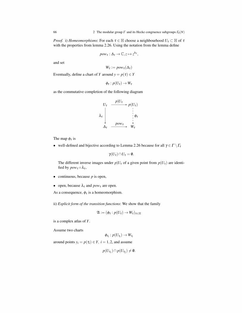
66 2 The modular group Γ and its Hecke congruence subgroups Γ0(N)
Proof. i) Homeomorphisms: For each τ ∈ H choose a neighbourhood Uτ ⊂ H of τ
with the properties from lemma 2.26. Using the notation from the lemma define
powτ : ∆τ → C,z 7→ zhτ ,
and setWτ := powτ(∆τ)
Eventually, define a chart of Y around y = p(τ) ∈ Y
φτ : p(Uτ)→Wτ
as the commutative completion of the following diagram
Uτ p(Uτ)
∆τ Wτ
p|Uτ
λτ
powτ
φτ
The map φτ is
• well-defined and bijective according to Lemma 2.26 because for all γ ∈ Γ \Γτ
γ(Uτ)∩Uτ = /0.
The different inverse images under p|Uτ of a given point from p(Uτ) are identi-fied by powτ λτ ,
• continuous, because p is open,
• open, because λτ and powτ are open.
As a consequence, φτ is a homeomorphism.
ii) Explicit form of the transition functions: We show that the family
A := (φτ : p(Uτ)→Wτ)τ∈H
is a complex atlas of Y .
Assume two chartsφτi : p(Uτi)→Wτi
around points yi = p(τi) ∈ Y, i = 1,2, and assume
p(Uτ1)∩ p(Uτ2) 6= /0.

2.3 Modular curves X(Γ0(N)) as compact Riemann surfaces 67
To simplify the subscripts we set
Ui :=Uτi ,φi := φτi ,λi := λτi ,hi := hτi ,Wτi :=Wi, i = 1,2.
Consider a pointx ∈ p(U1)∩ p(U2),
see Figure 2.6.

68 2 The modular group Γ and its Hecke congruence subgroups Γ0(N)
Fig. 2.6 Transition functions of Y

2.3 Modular curves X(Γ0(N)) as compact Riemann surfaces 69
We show that the transition function
φ2,1 := φ2 φ−11
is holomorphic in a neighbourhood of φ1(x) ∈W1 ⊂ C: By definition of φi twopoints τi ∈Ui, i = 1,2, exist with
λi(τi)hi = φi(x), i = 1,2.
They satisfy τ2 = γ(τ1) for a suitable γ ∈ Γ . Hence for q ∈ C in a neighbourhoodof φ1(x) the transition functions attains the value
φ2,1(q) =((λ2 γ λ
−11 )(q1/h1)
)h2
We have to prove: Taking the h1-root does not prevent the holomorphy of the map.
iii) Holomorphy of the transition functions: We prove the non-trivial case h1 > 1,i.e. we assume that the orbit x ∈ X is elliptic.
• Case φ1(x) = 0 ∈W1, i.e. τ1 = τ1:
The pointτ1 = τ1
is elliptic. Therefore also τ2 = γ(τ1) ∈U2 is elliptic. Because τ2 is the onlyelliptic point in U2 we obtain τ2 = τ2, and
τ2 = γ(τ1) and h := h2 = h1.
By construction of λi, i = 1,2, the composition of fractional lineartransformations
λ2 γ λ−11
is a fractional linear transformation of P1 mapping 0 to 0 and ∞ to ∞. Thereforea matrix
A =
(a bc d
)∈ GL(2,C)
exists withλ2 γ λ
−11 = A
andA · (0 1)> = (0 1)>, A · (1 0)> = (1 0)>.
With respect to the injection
C −→ P1, z 7→ (z : 1),
– the vector (0 1)> ∈ C2 represents the point (0 : 1) ∈ P1 and the point 0 ∈ C,

70 2 The modular group Γ and its Hecke congruence subgroups Γ0(N)
– while the vector (1 0)> ∈ C2 represents the point (1 : 0) ∈ P1 and the point∞ ∈ C∪∞.
As a consequence
A =
(a 00 d
)and
φ2,1(q) =((λ2 γ λ
−11 )(q1/h)
)h=(
A(q1/h))h
= ((a ·q1/h)/d)h = (a/d)h ·q.
Therefore φ2,1 is linear, and hence holomorphic in a neighbourhoodof 0 = φ1(x).
• Case φ2(x) = 0 ∈W2, i.e. τ2 = τ2:
The previous case shows the holomorphy of φ1,2 in a suitable neighbourhood.Because the map is bijective, its inverse φ2,1 is holomorphic.
• Case φ1(x) ∈W1 arbitrary, i.e. τ1 ∈U1 arbitrary:
We reduce this case to the other two cases. Choose τ3 ∈D with p(τ3) = x andconsider the chart
φτ3 : Uτ3 →Wτ3
with the shorthandU3 :=Uτ3 ,φ3 := φτ3 ,W3 :=Wτ3 .
In a suitable neighbourhood W of x with
W ⊂ (p(U1)∩ p(U2)∩ p(U3))
we haveφ1,2 = φ1,3 φ3,2.
The right-hand side is holomorphic due to part i) and ii). Therefore φ1,2 isholomorphic, q.e.d.
The important steps in the proof of Proposition 2.27 and its prerequisites:
• The modular group acts properly.
• Isotropy groups act as rotations (Lemma of Schwarz).
• Suitable fractional-linear maps λ : H '−→ ∆ .

2.3 Modular curves X(Γ0(N)) as compact Riemann surfaces 71
The upper half-plane has a canonical boundary point, the point ∞. The extension ofthe group action from Remark 2.8 shows that one has to consider also the rationalline Q, but not R\Q, as part of the boundary.When extending the Euclidean topology of H to a topology on H∗, one has todefine the neighbourhoods in H∗ of the additional points from
Q∪∞.
First, surprisingly as a neighbourhood basis of ∞ ∈H∗ one does not take thecomplements of compact sets in C as one does for the point
∞ ∈ P1
from the Riemann sphere, alias projective space. Instead one takes the sets
z ∈ C : Im z > R∪∞, R > 0,
i.e. the complements of sets with bounded imaginary part. Secondly, one translatesneighbourhoods of ∞ to neighbourhoods of a rational q ∈Q by fractional-lineartransformations γ ∈ Γ with
γ(∞) = q.
The resulting neighbourhood basis of a point q ∈Q are disks in H with q a point onthe Euclidean boundary of the disk, see Figure 2.7. The second step is determinedby the requirement, that the modular group acts as group of homeomorphismson H∗. The new topology of H∗ induces on Q the discrete topology. Apparently thelatter is finer than the topology induced on Q by the Euclidean topology of R.
Fig. 2.7 Neighbourhoods of infinity and of some rational points from H∗, from [17, Fig. 2.5]
Theorem 2.28 (The modular curve of the modular group). Consider the actionof the modular group Γ on the extended upper half-plane

72 2 The modular group Γ and its Hecke congruence subgroups Γ0(N)
H∗ :=H∪Q∪∞.
according to Remark 2.8.
1. On the orbit spaceX := Γ \H∗
exists the structure of a compact Riemann surface such that the following dia-gram commutes with canonical projections p and p∗ and canonical injections inthe horizontal direction
H H∗
Y X
p p∗
2. The Riemann surface X is biholomorphic equivalent to P1.
Proof. i) Topology on H∗: Take as neighbourhood basis of ∞ for the topology on H∗the sets
UR := τ ∈H : Im τ > R∪∞, R > 0,
and as neighbourhood basis of
q := a/c ∈Q, gcd(a,c) = 1,
the sets
γ(UR), R > 0, γ =
(a ∗c ∗
)∈ Γ ,
becauseγ(∞) = q
due to Remark 2.8. These neighbourhood bases together with the open sets of Hgenerate a topology on H∗ with H⊂H∗ an open subspace.
Note. Because fractional linear transformations from Γ take lines to circles or linesthe neighbourhoods of γ(UN) are circles tangent to the real axis at the distinguishedpoint a/c ∈Q. Hence neighbourhoods of ∞ and of rational points are completelydifferent from their counterpart with respect to the Euclidan topology, seeFigure 2.7.
ii) Hausdorff quotient topology on Γ \H∗: We provide the set
X := Γ \H∗
with the quotient topology with respect to the canonical projection
2.3 Modular curves X(Γ0(N)) as compact Riemann surfaces 73
p∗ : H∗→ X .
Then p∗ is an open map: The proof is the same as the corresponding proof forLemma 2.20. The proof uses only the fact that the quotient arises from a groupaction.
In order to show that X is Hausdorff we consider two points
xi = p∗(τi) ∈ X , τi ∈H∗, i = 1,2, and assume x1 6= x2.
We distinguish the following cases:
• τ1 ∈H, τ2 ∈Q∪∞: W.l.o.g. τ2 = ∞. For each
γ =
(a bc d
)∈ Γ
the formula
Im γ(τ) =Im τ
|c · τ +d|2=
Im τ
(c ·Re τ +d)2 + c2 · (Im τ)2 ≤
≤ Im τ ·
1d2 c = 0
1c2 · (Im τ)2 c 6= 0
≤
Im τ c = 01
Im τc 6= 0
≤ maxIm τ,1/Im τ
showsIm γ(τ)≤ maxIm τ,1/(Im τ),
independently from γ . Therefore a relatively compact neighbourhood
U1 ⊂⊂H
of τ1 and a neighbourhoodU2 ⊂H∗
of τ2 = ∞ exist such that for all γ ∈ Γ
γ(U1)∩U2 = /0.
As a consequencep∗(U1)∩ p∗(U2) = /0.
• τ1,τ2 ∈H: This case has been considered already by Corollary 2.25.
iii) Compactness of X : Denote by DH ⊂H the closure of D with respect to H.
Then
74 2 The modular group Γ and its Hecke congruence subgroups Γ0(N)
D := DH∪∞ ⊂H∗
is compact with respect to H∗: Consider an open covering (Ui)i∈I of D . If ∞ ∈Ui0then for suitable R > 0:
τ ∈DH
: Im τ > R∪∞ ⊂Ui0 .
The remaining setτ ∈D
H: Im τ ≤ R
is compact in H, and therefore covered by a finite subcovering of (Ui)i∈I . As aconsequence X is compact as continuous image via p∗ of the compact set
D ⊂H∗.
One has
Y = X \p∗(∞).
Therefore Y ⊂ X is an open subset.
iv) Charts of the modular curve: In order to define a chart
φ∞ : p∗(U∞)→W∞
around the cuspx = p∗(∞) ∈ X
we consider the neighbourhood of ∞ ∈H∗
U∞ :=U2 = τ ∈H : Im τ > 2∪∞.
We define
pow∞ : U∞→ ∆ , τ 7→
e2πi·τ if τ 6= ∞
0 if τ = ∞
and setW∞ := pow∞(U∞)⊂ ∆ .
For two points τi ∈U∞, i = 1,2,
p∗(τ2) = p∗(τ1) ⇐⇒ τ2 = γ(τ1) for a suitable γ ∈ Γ
⇐⇒ τ2 = τ1 +m for a suitable m ∈ Z, due to Theorem 2.16,
⇐⇒ pow∞(τ2) = pow∞(τ1).
We define the chart φ∞ as the commutative completion of the diagram

2.3 Modular curves X(Γ0(N)) as compact Riemann surfaces 75
U∞ p∗(U∞)
W∞
p∗|U∞
φ∞pow∞
One shows analogously to the proof of Proposition 2.27 that the map φ∞ is a home-omorphism.
Eventually we have to show that the charts of Y and the chart φ∞ are compatible, Itsuffices to prove the compatibility of the chart
φ∞ : p∗(U∞)→W∞
around p∗(∞) with the chart
φτ : p(Uτ) = p∗(Uτ)→Wτ
around an arbitrary point p(τ), τ ∈H. We may assume that Uτ does not contain anelliptic point, and therefore that
φτ (p∗|Uτ)
is injective and biholomorphic. Hence the transition function of the two charts isholomorphic.
v) Modular curve X ' P1: The image of the fundamental domain
Y = p(D)
is homeomorphic to the plane C: Identify points on the left and right boundary ofD and equivalent points of D on the left part of the unit circle and on the right part.Therefore the compactification of Y is homeomorphic to the 1-point compactifica-tion of C, i.e. X is homeomorphic to S2. The only complex structure on the sphere S2
is the complex projective space P1(C), cf. [63], q.e.d.
For the biholomorphy
X ' P1
a formal proof will be given in Corollary 3.16. This second proof uses the modularinvariant j from the theory of modular forms.

76 2 The modular group Γ and its Hecke congruence subgroups Γ0(N)
Definition 2.29 (Modular curve of Γ ). The compact Riemann surface from Theo-rem 2.28
X(1) := X(Γ ) := Γ \H∗
is named the modular curve of Γ or simply the modular curve.
An analogous construction of a modular curve can be made for each congruencesubgroup Γ0(N)⊂ Γ .
Remark 2.30 (Modular curves of the congruence subgroups). Generalizing the con-struction of the modular curve
X(1) = Γ \H∗
from Theorem 2.28 one can introduce for each Hecke congruence subgroup
Γ0(N)⊂ Γ , N ∈ N,
a complex structure on the orbit space
X0(N) := Γ0(N)\H∗ = (Γ0(N)\H) ∪Cusp(Γ0(N)),
see [17, Prop. 2.4.2ff.] The resulting compact Riemann surface X0(N) is named themodular curve of Γ0(N).
1. Branched covering of modular curves: The inclusion of groups
Γ0(N) −→ Γ (1)
induces a holomorphic branched covering
f : X0(N)−→ X(1)
of compact Riemann surfaces. The covering has degree
deg f = [Γ : Γ0(N)] = N ·∏p|N
(1+
1p
),
see [17, Exerc. 3.1.1] and Proposition 2.14.
2. Genus of modular curves: The Riemann-Hurwitz formula, e.g., [63], applied tothe covering
f : X0(N)−→ X(1)' P1
computes the genus of the modular curves of the Hecke congruence subgroupsas

2.3 Modular curves X(Γ0(N)) as compact Riemann surfaces 77
g(X0(N)) = 1+b( f )
2−deg f
withb( f ) = ∑
x∈X0(N)
b( f ; x)
the total branching order of f .
A detailed investigation of the elliptic points and of the cusps of the actionof Γ0(N) shows the genus formula
g(X0(N)) = 1+deg f
12−
ε2
4−
ε3
3−
ε∞
2
with ε2, ε3 and ε∞ denoting the number of elliptic points of respectively period 2and 3 and the number of cusps of the action of Γ0(N), see [17, Theor. 3.1.1].
The ε-constants can be computed as
ε∞ = ∑d|N
Φ(gcd(d,N/d)),
see Example 2.11, and ε2 and ε3 are the numbers of solutions in Z/NZ of theequations respectively
x2 +1 = 0 and x2− x+1 = 0.
Using the quadratic residue symbol for n∈−1,−3 and extended to all primes p
(−1p
):=
0 if p = 21 if p≡ 1 mod 4−1 if p≡ 3 mod 4
and (−3p
):=
0 if p = 31 if p≡ 1 mod 3−1 if p≡ 2 mod 3
one obtains, see [17, Cor. 3.7.2, Exerc. 3.7.6] and [53, Theor. 1.43]:
ε2 =
∏p|N
(1+(−1p
))if 4 - N
0 otherwise
and

78 2 The modular group Γ and its Hecke congruence subgroups Γ0(N)
ε3 =
∏p|N
(1+(−3p
))if 9 - N
0 otherwise
3. Estimate of the genus g(X0(N)): As a corollary of the genus formula the constantsfrom part 2) satisfy the estimate
2 ·g(X0(N))−2+ε2
2+
2ε3
3+ ε∞ > 0.
4. Modular curves of prime level: For a prime p ∈ N and k := p+ 1 the modularcurve X0(p) has the genus
g(X0(p)) =
⌊k
12
⌋−1 if k ≡ 2 mod 12
⌊k
12
⌋otherwise
In particular,
g(X0(2)) = 0, g(X0(11)) = 1, g(X0(13)) = 0 and g(X0(17)) = 1
5. Numerical example: See the PARI-file “modular curve as covering”. For thecomputation of the extended quadratic residue symbol PARI provides the com-mand
kronecker(a,p).
The Kronecker symbol is defined for arbitrary integer a∈Z and arbitrary primesincluding p = 2 by extending the Legendre symbol:
• Odd prime p:
kronecker(a, p) :=(
ap
)for odd p
• Even prime p = 2:
kronecker(a,2) :=
0 if a even(−1)(a
2−1)/8 otherwise
The Kronecker symbol satisfies
• Odd prime p:
kronecker(−4, p) =(−4p
)=
(2p
)2
·(−1p
)=
(−1p
)

2.3 Modular curves X(Γ0(N)) as compact Riemann surfaces 79
• Even prime p = 2:
kronecker(−4,2) = 0 =
(−12
)and kronecker(−3,2) =−1 =
(−32
)Hence
ε2 =
∏p|N (1+ kronecker(−4, p)) if 4 - N
0 otherwise
and
ε3 =
∏p|N (1+ kronecker(−3, p)) if 9 - N
0 otherwise
Figure 2.8 shows the invariants of the covering
X0(p)−→ X(1)
for all primes p < 100.

80 2 The modular group Γ and its Hecke congruence subgroups Γ0(N)
Fig. 2.8 Modular curves X0(N)−→ X(1)

Chapter 3The algebra of modular forms
Modular forms are holomorphic functions on H distinguished by two properties:
1. On one hand, they have the modular group as group of symmetries.
2. On the other hand, they expand into a Fourier series around the point ∞ withrational Fourier coefficients after normalization.
The interplay of these two properties is coined “The magic of modular forms” [65].Therefrom arises a series of remarkable identities between the Fourier coefficientsof modular forms. In many cases these identities imply interesting statements aboutarithmetic functions. We will see examples in Section ?? and Chapter 6.
In general, one introduces modular forms as functions on H with a certain trans-formation behaviour with respect to the action of the modular group or its con-gruence subgroups. The basic examples are the Eisenstein series, see Section 3.2.A meromorphic quotient of certain modular forms is the modular invariant j, seeDefinition 3.15, a key object of the whole theory. From a more abstract point ofview, modular forms are differential forms on the modular curves, which are com-pact Riemann surfaces, see Theorem 3.17. The Riemann-Roch theorem computesthe dimensions of the different vector spaces of modular forms.
3.1 Modular forms and cusp forms
Modular forms are holomorphic functions on H which transform in a simple man-ner under the operation of the congruence subgroups Γ0(N) and extend to H∗ ina certain holomorphic way. These functions have a discrete non-Abelian group ofsymmetries.
81

82 3 The algebra of modular forms
We introduce modular forms as analytical objects which are invariant undertransformation of the modular group Γ or its Hecke subgroups Γ0(N). In a sec-ond step, such invariant objects can be considered analytical objects on the modularcurves X0(N). Because the modular curves are compact Riemann surfaces one can-not expect interesting objects when restricting to invariant holomorphic functions.Instead one has to consider more general holomorphic and meromorphic differentialforms.
We start from the general context of representation theory of the group Γ , i.e. weintroduce a Γ -action on certain vector spaces of holomorphic differential forms.
Proposition 3.1 (Γ -invariant differential forms). Denote by
W 1 := H0(H,Ω 1H)
the vector space of holomorphic differential forms on the upper half-plane H.
1. The mapΦ
1 : W 1×Γ →W 1, (ω,γ) 7→Φ1(ω,γ) := γ
∗ω,
is a Γ -right action. For
γ =
(a bc d
)∈ Γ , ω = f dτ ∈W 1 and τ ∈H
holds
Φ1(ω,γ)(τ) := (γ∗ω)(τ) = ( f γ)(τ)
dτ
(cτ +d)2
2. For even k ∈ N set
Ωk/2 := Ω
⊗k/2H and W k/2 := H0(H,Ω k/2)
andΦ
k/2 : W k/2×Γ →W k/2, (ω,γ) 7→Φk/2(ω,γ) := γ
∗ω.
For
γ =
(a bc d
)∈ Γ , ω = f (dτ)k/2 ∈W k/2 and τ ∈H
holds
Φk/2(ω,γ)(τ) := ((γ ∗)k/2
ω)(τ) = ( f γ)(τ)(dτ)k/2
(cτ +d)k
3. For even k ∈ N,
γ =
(a bc d
)∈ Γ and ω = f (dτ)k/2 ∈W k/2

3.1 Modular forms and cusp forms 83
holds the equivalence which characterizes invariant differential forms:
γ∗ω = ω ⇐⇒ f (τ) = ( f γ)(τ)
1(cτ +d)k for all τ ∈H.
Note. In the context of modular forms Ω k/2 denotes the tensor product of Ω 1 notthe exterior product.
Proof. 1. We have
Φ1(ω,γ1 · γ2) = (γ1 · γ2)
∗ω = γ
∗2 (γ ∗1 ω) = Φ
1(Φ1(ω,γ1),γ2)
Moreover
(dγ)(τ) = d
(aτ +bcτ +d
)=
a(cτ +d)− (aτ +b)c(cτ +d)2 dτ =
1(cτ +d)2 dτ
Therefore
(Φ1( f dτ,γ))(τ) := (γ ∗( f dτ))(τ) = f (γ(τ)) (dγ)(τ) = ( f γ)(τ)dτ
(cτ +d)2
2. For even k > 2 the proof is analogous by applying the derivation separately foreach tensor factor dτ , q.e.d.
Proposition 3.1 shows: For even k ∈ N the invariant differential forms from thefixed space of the Γ -representation
f dτk/2 ∈ (W k/2)Γ
are characterized by holomorphic coefficient functions f ∈ O(H) satisfying
f (τ) = ( f γ)(τ) ·1
(cτ +d)k
for all
γ =
(a bc d
)∈ Γ and τ ∈H.
If these coefficent functions extend holomorphically to ∞ ∈H∗ they will be namedmodular functions of weight = k. The factors
1(cτ +d)k
from their transformation law will be isolated and termed factors of automorphy,see Definition 3.3.

84 3 The algebra of modular forms
For the translation
T :=(
a bc d
):=(
1 10 1
)∈ Γ0(N)
the factors of automorphy satisfy for all τ ∈H
1cτ +d
= 1.
Hence
T ∗( f (dτ)k/2) = f (dτ)k/2 ⇐⇒ f (τ +1) = f (τ) for all τ ∈H,
and the latter equality means that the function f has the period = 1. Hence f expandsinto a convergent Fourier series
f (τ) = f (q) =∞
∑n=−∞
an ·qn, q = e2πi·τ ,
similar to the trigonometric function
cos(2πz) =12(e2πi·z + e−2πi·z) .
The holomorphic mapH→ ∆
∗,τ 7→ e2πiτ ,
surjects to the punctured unit disk
∆∗ := z ∈ C : 0 < |z|< 1.
Here neighbourhoods of ∞∈H∗ with respect to the topology of H∗ from Theorem 2.28are mapped to neighbourhoods of zero. A meromorphic function on H with period = 1induces a corresponding meromorphic function f on ∆ ∗ according to the followingdiagram
H C
∆ ∗
f
f
Set
f (q) := f (τ) =∞
∑n=−∞
an ·qn, q = e2πi·τ .

3.1 Modular forms and cusp forms 85
Definition 3.2 (q-expansion and Fourier coefficients). Consider a meromorphicfunction f on H invariant with respect to the operation of T and the induced mero-morphic function f on ∆ ∗ with
f (q) := f (e2πiτ) := f (τ).
1. The function f is named meromorphic at ∞
• if f has an isolated singularity at 0 and
• if this singularity is a pole or a removable singularity.
2. If f is meromorphic at ∞ then the induced function f has a Laurent expansionaround 0
f (q) =∞
∑n=n0
an ·qn, q = e2πiτ ,
with a suitable n0 ∈ Z. The Laurent expansion is named the q-expansion of f ,and the elements (an)n≥n0 are the Fourier coefficients of f .
3. A function f , meromorphic at ∞, is named holomorphic at ∞ if n0 ∈ N, i.e.if 0 ∈ ∆ is a removable singularity of f . In this case one defines
f (∞) := f (0).
Note: For a meromorphic function f on H, invariant with respect to T :
f holomorphic at ∞ ⇐⇒ limIm τ→∞
| f (τ)|< ∞ ⇐⇒
⇐⇒ ∃ R > 0 : | f (τ)| bounded for Im τ ≥ R.
Modular forms will not be necessarily invariant under the operation of Γ0(N), butthey multiply with a factor of automorphy which is a holomorphic function withoutzeros. We define the concept in a slightly more general context.
Definition 3.3 (Factor of automorphy). Consider the left group action
Φ : GL(2,R)+×H→H, (γ,τ) 7→ γ(τ) :=aτ +bcτ +d
, γ =
(a bc d
),
which extends the group action of the modular group Γ to GL(2,R)+. The map
h : GL(2,R)+×H→H, h(γ,τ) := cτ +d,
is named the factor of automorphy of Φ .
The translation T ∈ SL(2,Z) has the factor of automorphy h(T,−) = 1.

86 3 The algebra of modular forms
Lemma 3.4 (Transformation of the factors of automorphy).
1. The factors of automorphy satisfy the composition rule
h(B ·A,τ) = h(B, A(τ)) ·h(A,τ); A,B ∈ GL(2,R)+, τ ∈H.
2. Consider the vector space
V := f : H−→ C
of complex-valued functions on H. For any k ∈ Z the map
V ×GL(2,R)+ −→V, ( f ,γ) 7→ f [γ]k,
withf [γ]k(τ) := f (γ(τ)) ·h(γ,τ)−k · (det γ)k−1, τ ∈H,
is a right group action of GL(2,R)+ on the vector space V .
In the definition of f [γ]k from Lemma 3.4 the exponent of det γ is not uni-form in the literature. We use the exponent (k − 1) from [17, Exerc. 1.2.11],while [35, Chap. III, §3] uses the exponent k/2. The choice of the exponent (k−1)will later simplify Definition 5.10.
Note that in Lemma 3.4 the group GL(2,R)+ is written on the right-hand side ofthe vector space V .
Proof. Consider A,B ∈ GL(2,R)+ and τ ∈H.
1.
A ·(
τ
1
)=
(A(τ)
1
)·h(A,τ).
Here we distinguish between the matrix product of A with a vector on the left-hand side and the fractional linear transformation A(τ) on the right-hand side.
Applying this identity to the product B ·A
(B ·A) ·(
τ
1
)=
((B ·A)(τ)
1
)·h(B ·A,τ).
Left-hand side:
B ·(
A ·(
τ
1
))= B ·
((A(τ)
1
)·h(A,τ)
)=
(B(A(τ))
1
)·h(B,A(τ)) ·h(A,τ).
Equating with the right-hand side gives for the lower row
h(B ·A,τ) = h(B,A(τ)) ·h(A,τ),

3.1 Modular forms and cusp forms 87
hence for the upper row(B ·A)(τ) = B(A(τ)).
2. Starting with the right-hand side we compute
(( f [B]k)[A]k)(τ) = ( f [B]k)(A(τ)) ·h(A,τ)−k(det A)k−1 =
= f (B(A(τ))) ·h(B,A(τ))−k ·h(A,τ)−k · (det B)k−1 · (det A)k−1 =
= f ((B ·A)(τ)) ·h(B ·A,τ)−k · (det (B ·A))k−1 = f [B ·A]k(τ).
Here the penultimate equality holds due the result from part 1) and due to theequality
(B ·A)(τ) = B(A(τ))
from the proof of part i). Hence
f [B ·A]k = ( f [B]k)[A]k, q.e.d.
Remark 3.5 (Meromorphy and holomorphy at the cusps). The Fourier expansionfrom Definition 3.2 is well-defined for holomorphic functions f : H −→ C wich areinvariant with respect to the translation T . The modular group Γ has only a sin-gle cusp, the orbit comprising ∞ and all rationals q ∈ Q. But Hecke congruencesubgroups Γ0(N), N ≥ 2, have several cusps, each comprising a different subset ofrationals q ∈ N.
Fix a Hecke congruence subgroup Γ0(N), a weight k ∈ Z, and a rational q =ac∈Q.
How to extend a holomorphic function
f : H−→ C
withf [γ]k = f
for all γ ∈ Γ0(N) to the point q ∈Q in a meromorphic or holomorphic way?
We consider the canonical surjective group homomorphism
Γ −→ PSL(2,Z) := Γ /±1, α 7→ α.
The image Γ ∞ ⊂ PSL(2,Z) of the isotropy group Γ∞ ⊂ Γ is generated by thetranslation:
Γ ∞ =< T >= T k : k ∈ Z ' Z
If α ∈ Γ withq = α(∞)

88 3 The algebra of modular forms
thenΓ0(N)q ' α
−1 · Γ0(N)q ·α ⊂ Γ∞
orΓ0(N)q ' α
−1 · Γ0(N)q ·α ⊂ Γ ∞ ' Z
For
α =
(a bc d
)define γ := α ·T N ·α−1 =
(∗ ∗−Nc2 ∗
)∈ Γ0(N)q
Then γ ∈ Γ0(N)q. Because < T N > ⊂ Γ∞ is a subgroup of finite index, the sameholds for
< γ > ⊂ Γq and for < γ > ⊂ Γ q
We obtain
1≤ hq := [Γq : Γ0(N)q] = [Γ q : Γ0(N)q]< ∞
Lemma 3.4 shows
( f [α]k)[T hq ]k = f [α ·T hq ]k = f [γ ·α]k = ( f [γ]k)[α]k = f [α]k
Hence f [α]k is invariant under T hq and has a Fourier series
( f [α]k)(τ) =∞
∑n=−∞
an · qn, q := e2πi·τ/hq
The function f [α]k is named meromorphic respectively holomorphic at ∞ iff f [α]khas at q = 0 at most a pole respectively a removable singularity. Note that the orderof f [α]k at q = 0 does not depend on the choice of α .
The fundamental object of the whole theory is the modular form. We intro-duce modular forms of the modular group Γ respectively its Hecke congruencesubgroups Γ0(N) as the coefficient functions of the invariant differential forms fromProposition 3.1 which extend to ∞ ∈ H∗. It turns out that modular forms are mero-morphic differential forms on the modular curve X0(N), see Theorem 3.17.
Definition 3.6 (Modular forms and automorphic forms).
1. Modular forms and automorphic forms of the modular group: Consider aninteger k ∈ Z and a meromorphic function f on H.
• The function f is weakly modular of weight k with respect to Γ if for all γ ∈ Γ
and for all τ ∈H
f (γ(τ)) ·1
(cτ +d)k = f (τ), γ =
(a bc d
).

3.1 Modular forms and cusp forms 89
• The function f is an automorphic form of weight k with respect to Γ if f isweakly modular of weight k and meromorphic at ∞.
• The function f is a modular form of weight k with respect to Γ if f is weaklymodular of weight k, holomorphic on H and holomorphic at ∞.
• A modular form f of weight k vanishing at all points of the cusp of Γ , i.e.
f (∞) = 0
is a cusp form of weight k with respect to Γ .
• An automorphic function with respect to Γ is an automorphic form of weight = 0,i.e. satisfying
f γ = f .
Similarly, a modular function is a modular form of weight = 0.
• On denotes byAk(Γ )⊃Mk(Γ )⊃ Sk(Γ )
the vector spaces of automorphic forms with respect to Γ of weight k, thesubspace of modular forms, and the subspace of cusp forms.
2. Modular forms of congruence subgroups: Consider a congruence subgroup Γ0(N)with a positive integer N ∈ N∗.
• A modular form of weight k ∈ Z, k ∈ Z, with respect to Γ0(N) is a holomor-phic function
f : H→ C
with the following properties: For all γ ∈ Γ0(N) holds
f [γ]k = f ,
and for all α ∈ Γ the function f [α]k is holomorphic at ∞ in the sense ofRemark 3.5.
• A modular form f of weight k ∈ Z, k ∈ Z, with respect to Γ0(N) is nameda cusp form of weight k ∈ Z with respect to Γ0(N) if for all α ∈ Γ thefunction f [α]k is holomorphic at ∞, and its Fourier series in the sense of Re-mark 3.5 vanishes at q = 0.
3. Automorphic forms of congruence subgroups: An automorphic form of weight k, k ∈ Z,with respect to Γ0(N) is a meromorphic function on H with the following prop-erties: For all γ ∈ Γ0(N) holds
f [γ]k = f ,

90 3 The algebra of modular forms
and for all α ∈ Γ the function f [α]k is meromorphic at ∞ in the sense ofRemark 3.5.
We denote byAk(Γ0(N))⊃Mk(Γ0(N))⊃ Sk(Γ0(N))
the complex vector space of respectively automorphic forms, modular forms, andcusp forms of weight k with respect to Γ0(N).
Definition 3.6, part 2) and 3) generalize part 1): For γ ∈ Γ holds det γ = 1, hence
f [γ]k(τ) = ( f γ)(τ) ·1
(cτ +d)k
Note that Definition 3.6 uses the weight convention from [17, Chap. 1.1]. Somesources use a different weight convention. In the literature also the notation to dis-criminate between modular functions and modular forms is not uniform.
As a consequence of Theorem 2.16 and Lemma 3.4 it is sufficient to require inDefinition 3.6, part 1) the transformation law only for the two generators S,T of Γ .
Remark 3.7 (Modular forms of odd weight). A modular form of a congruence sub-group Γ0(N), N ∈N, of odd weight k ∈ Z satisfies for all τ ∈H and for the particularelement
γ =
(−1 0
0 −1
)∈ Γ0(N)
the equation
f (τ) = f [γ]k(τ) = f (γ(τ)) · (−1)k = f (τ) · (−1)k.
Therefore f = 0 is the only modular function of Γ0(N) of odd weight.
3.2 Eisenstein series and the algebra of modular forms of Γ
We will now construct for the modular group Γ = SL(2,Z) explicit modularforms Gk of even weight k≥ 4 and a distinguished holomorphic function G2, whichbehaves in a different way under the Γ -action. To achieve the construction weneed the convergence of certain infinite series. Lemma 3.8 provides the necessaryprerequisites.

3.2 Eisenstein series and the algebra of modular forms of Γ 91
The whole section will use the unbranched covering projection
q : H−→ ∆∗, τ 7→ q(τ) := e2πi·τ ,
to study the number theoretic properties of modular forms f by considering theFourier coefficients of their Fourier expansion
f (q) =∞
∑n=0
an ·qn
Lemma 3.8 (Fourier series and partial fraction). Assume k ∈ N. Consider τ ∈ Cand set
q := e2πi·τ .
1. For k ≥ 2 and Im τ 6= 0
∑n∈Z
1(τ +n)k =
(−2πi)k
(k−1)!·
∞
∑r=1
rk−1 ·qr Im τ > 0
(−1)k ·∞
∑r=1
rk−1 ·q−r Im τ < 0
2. The double series∞
∑m,d=1
d ·qmd
satisfies the prerequisites of the rearrangement theorem, i.e. there exists a con-stant K such that for all finite subsets A, B⊂ N∗ holds
∑m∈A,d∈B
d · |q|md ≤ K
3. For even k ≥ 2, Im τ > 0,
∑m∈Z∗
(∑n∈Z
1(mτ +n)k
)=
2 (2πi)k
(k−1)!·
∞
∑n=1
σk−1(n) qn
is absolutely convergent.
Here for each k ≥ 2 the arithmetic function
σk−1 : N∗→ N∗, σk−1(n) := ∑d|n
dk−1,
adds the (k−1)-powers of the positive integer divisors of n.
Proof. 1. i) We first consider the case Im τ > 0. The proof compares the partialfraction and the Fourier expansion of the cotangent function.
92 3 The algebra of modular forms
• Partial fraction, see [62]:
π · cot(πτ) =1τ+
∞
∑m=1
(1
τ +m+
1τ−m
)
• Fourier series
π · cot(πτ) = πcos(πτ)
sin(πτ)= (−iπ) ·
1+q1−q
=−πi−2πi∞
∑m=1
qm.
Here the second equality results from the Euler formulas
cos πτ =12(eiπτ + e−iπτ) and sin πτ =
12i(eiπτ − e−iπτ)
which imply
cot(πτ) = i ·eiπτ + e−iπτ
eiπτ − e−iπτ= i ·
q+1q−1
= (−i) ·1+q1−q
The third equality uses the geometric series
1+q1−q
= (1+q)∞
∑m=0
qm = 1+2∞
∑m=1
qm
which is absolutely convergent because |q|< 1 due to τ ∈H.
Equating both expansions gives
1τ+
∞
∑m=1
(1
τ +m+
1τ−m
)=−πi−2πi
∞
∑m=1
qm,
and successive (k−1)-times differentiation with respect to τ shows
∑m∈Z
1(τ +m)k =
(−2πi)k
(k−1)!·
∞
∑m=1
mk−1 qm.
ii) For Im τ < 0 we use
(τ +n)k = (−1)k · (−τ−n)k
Hence
∑n∈Z
1(τ +n)k = (−1)k ·∑
n∈Z
1(−τ−n)k = (−1)k ·∑
n∈Z
1(−τ +n)k
Part i) applied to −τ implies

3.2 Eisenstein series and the algebra of modular forms of Γ 93
(−1)k ·∑n∈Z
1(−τ +n)k =
(−2πi)k
(k−1)!· (−1)k ·∑
r=1rk−1 ·q−r
which proves the claim.
2. Consider τ ∈H with q := e2πiτ real and 0 < q < 1.
For any real x ∈ [0,1[ the geometric series satisfies∞
∑d=0
xd =1
1− x
Taking the derivative and multiplying by x shows
∞
∑d=1
d · xd =x
(1− x)2
For arbitrary but fixed m≥ 1 set x := qm < 1
∞
∑m=1
(∞
∑d=1
d ·qmd
)=
∞
∑m=1
(∞
∑d=1
d · (qm)d
)=
∞
∑m=1
qm
(1−qm)2
The last series is convergent because for fixed q
limm→∞|1−qm|2 = 1.
Set
K :=∞
∑m=1
qm
(1−qm)2
As a consequence∑
m∈A,d∈Bd ·qmd ≤ K.
For arbitrary τ ∈H we have
q := e2πiτ with 0≤ |q|< 1
Hence w.l.o.g. we may assume q real with 0≤ q < 1, which proves the claim.
3. We split the exterior summation ∑m∈Z∗
into
∑m<0
where Im(mτ)< 0 and ∑m>0
where Im(mτ)> 0.
Due to part 1) for each m ∈ Z∗ exists the interior series

94 3 The algebra of modular forms
∑n∈Z
1(mτ +n)k =
(2πi)k
(k−1)!·
∞
∑r=1
rk−1 ·q−rm if m < 0
∞
∑r=1
rk−1 ·qrm if m > 0
Hence for even k ≥ 2
∑m∈Z∗
(∑n∈Z
1(mτ +n)k
)= 2 ·
(2πi)k
(k−1)!·
∞
∑m=1
(∞
∑r=1
rk−1 ·qrm
).
The latter series is convergent: For k≥ 4 any rearrangement of the original doubleseries is permitted. For k = 2 the result of part 2) allows to apply the rearrange-ment theorem to the double series
∞
∑m,r=1
r ·qrm, |q|< 1.
We rearrange the series by changing the indices of summation from (m,r)to (n = rm,d|n):
∞
∑m=1
(∞
∑r=1
rk−1 ·qrm
)=
∞
∑n=1
(∑d|n
dk−1 ·qn
)=
∞
∑n=1
σk−1(n) ·qn.
Eventually for all even k ≥ 2
∑m∈Z∗
(∑n∈Z
1(mτ +n)k
)= 2 ·
(2πi)k
(k−1)!·
k
∑n=1
σk−1(n) ·qn, q.e.d.
Eisenstein series are the lattice constants of normalized lattices
Λ1,τ = Z ·1+Z · τ
when considered as functions of the argument τ ∈ H. Eisenstein series are explicitrepresentations of modular forms.
Theorem 3.9 (Eisenstein series, k ≥ 4). Consider an even integer k ≥ 4.
1. The Eisenstein series
Gk(τ) := ∑(c,d)∈Z2
′ 1(cτ +d)k
is absolutely and compactly convergent for τ ∈H.
The series defines a modular form Gk of Γ of weight k with
3.2 Eisenstein series and the algebra of modular forms of Γ 95
Gk(∞) = 2ζ (k).
Here
ζ (s) :=∞
∑n=1
(1/ns), Re s > 1,
denotes the Riemann ζ -function.
2. The Eisenstein series Gk ∈Mk(Γ ) has the Fourier expansion
Gk(τ) = 2ζ (k)+2(2πi)k
(k−1)!
∞
∑n=1
σk−1(n) ·qn, q = e2πiτ .
Proof. i) Convergence and transformation: For τ ∈ H consider the normalized lat-tice
Λτ := Z+Zτ
and for k ≥ 4 its lattice constants GΛτ ,k . Apparently
Gk(τ) := GΛτ ,k
The series GΛ ,k is absolute convergent due to Lemma 1.11, hence allows arbitraryrearrangement. With respect to the translation
T : H→H, τ 7→ T (τ) := τ +1,
we obtainGk(τ) = Gk(τ +1).
With respect to the reflection
S : H→H, τ 7→ S(τ) :=−1τ
we have
Gk(S(τ)) ·h(S,τ)−k =1τk ·Gk(−(1/τ)) =
1τk · ∑
(c,d)∈Z2
′ 1(−c(1/τ)+d)k = Gk(τ).
Because S and T generate the modular group, Lemma 3.4 implies for all γ ∈ Γ andfor all τ ∈H
Gk(τ) = Gk(γ(τ)) ·h(γ,τ)−k, i.e. Gk = Gk[γ]k
ii) Fourier expansion and holomorphy: We split the summation over
(c,d) ∈ Z2,(c,d) 6= (0,0),
into the simple sum for (c,d) with c = 0 and d ∈Z∗ and the double sum with c ∈ Z∗and d ∈ Z. Then Lemma 3.8, part 3) implies

96 3 The algebra of modular forms
Gk(τ) = ∑(c,d)∈Z2
′ 1(cτ +d)k = ∑
d∈Z∗
1dk + ∑
c∈Z∗,d∈Z
1(cτ +d)k =
= 2ζ (k)+2 (2πi)k
(k−1)!·
∞
∑n=1
σk−1(n) qn, q = e2πi·τ .
The Fourier expansion, a convergent power series, proves the holomorphy of Gk inH and at the point ∞, q.e.d.
In order to get rid of the transcendent values in the Fourier expansion of Gk onedivides by the value of the Riemann ζ -function.
Definition 3.10 (Normalized Eisenstein series). For even k ≥ 4 one defines thenormalized Eisenstein series
Ek :=Gk
2ζ (k)∈Mk(Γ )
Corollary 3.11 (Normalized Eisenstein series). For each k ≥ 4 all Fourier coeffi-cients of the normalized Eisenstein series are rational, more precisely
Ek(τ) = 1−2kBk·
∞
∑n=1
σk−1(n) ·qn ∈Mk(Γ ), q = e2πi·τ
Proof. 1. Euler relation of Bernoulli numbers: See [20, Kap. VII, Satz 4.1]. Werelate the cotangent function to the Bernoulli numbers (Bn)n∈N. The Bernoullinumbers are the generators of the power series
zez−1
=:∞
∑n=0
Bn
n!· zn.
We compute
cot z =cos zsin z
= i ·eiz + e−iz
eiz− e−iz = i ·e2iz +1e2iz−1
= i+2i
e2iz−1
and use the vanishing of Bernoulli numbers with odd index≥ 3 and B0 = 1, B1 =−1/2
z·cotz= iz+2iz
e2iz−1= iz+1−
2iz2+
∞
∑µ=1
B2µ
(2µ)!·(2iz)2µ = 1+
∞
∑µ=1
(−1)µ22µ
(2µ)!·B2µ ·z2µ
• On one hand from the definition of the Bernoulli numbers - replacing z by πz -
πz · cot(πz) = 1+∞
∑µ=1
(−1)µ ·22µ
(2µ)!·π2µ ·B2µ · z2µ

3.2 Eisenstein series and the algebra of modular forms of Γ 97
• On the other hand the partial fraction of the cotangent function
πz · cot(πz) = 1+ z∞
∑ν=1
2zz2−ν2
and the geometric series
1z2−ν2 =−
1ν2 ·
∞
∑µ=0
(z2
ν2
)µ
imply
πz · cot(πz) = 1+2z2 ·∞
∑ν=1
(−
1ν2 ·
∞
∑µ=0
(z2
ν2
)µ)=
= 1−2∞
∑µ=1
(∞
∑ν=1
1ν2µ
)z2µ
Comparing the coefficients of both series representing
πz · cot(πz)
implies the Euler relation
2 ·ζ (2µ) := 2 ·∞
∑ν=1
1ν2µ
= (−1)µ+1 22µ
(2µ)!·π2µ ·B2µ
2. Rationality of the Fourier coefficients: The Fourier expansion of the Eisensteinseries Gk from Theorem 3.9 and Part 1) show
Ek(τ) :=Gk(τ)
2ζ (k)= 1−
2kBk·
∞
∑n=1
σk−1(n) ·qn ∈Mk(Γ ).
All Bernoulli numbers are rational due to the recursion formula for N ∈ N∗
N
∑n=0
(N +1
n
)·Bn = 0 with B0 = 1.
As a consequence, all Fourier coefficients of Ek are rational, q.e.d.
Concerning the first values of Bernoulli numbers(k,ζ (k),Bk,−
2kBk
)

98 3 The algebra of modular forms
one has
(2,π2/6,1/6,−24)
(4,π4/(2 ·32 ·5),−1/30,240)
(6,π6/(33 ·5 ·7),1/42,−504)
(8,π8/(2 ·33 ·52 ·7),−1/30,480)
(10,π10/(35 ·5 ·7 ·11),5/66,−264)
(12, 691 ·π12/(36 ·53 ·72 ·11 ·13),−691/2730,65520/691)
For k ∈ 4,6,8 the numerical value of Bk implies that all Fourier coefficientsof Ek are not only rational but are integers.
Remark 3.12 (Eisenstein series).
1. Rationality of the Fourier coefficients: The result from Corollary 3.11 is remark-able: The invariance of the holomorphic function Ek under the right action ofthe modular group implies the rationality of the Fourier coefficients of Ek. TheFourier coefficients of these holomorphic functions are not arbitrary numbersfrom C but rationals from Q. This rationality is the reason for the “magic ofmodular forms” revealed by later applications. See also Proposition 3.14.
2. Weight k ≥ 4: For even k > 2 the Eisenstein series Gk relate to the latticeconstants GΛ ,k of an arbitrary lattice with positively oriented basis
Λ = Zω1 +Zω2
as follows: Set τ := ω2/ω1 ∈H. Then
GΛ ,k =1
ω k1
Gk(τ).
3. Weight k = 2: Similar to the series
∞
∑n=1
(−1)n−1
n
in one dimension, in two dimensions the series
∑(m,n)∈Z2
′ 1(mτ +n)2
3.2 Eisenstein series and the algebra of modular forms of Γ 99
is not absolutely convergent. Anyhow, in both cases some specific orders of sum-mation provide certain finite values. In the 2-dimensional case we define theEisenstein series
G2(τ) := 2 ·∞
∑n=1
1n2 + ∑
m∈Z∗
(∑n∈Z
1(mτ +n)2
), τ ∈H.
Lemma 3.8, part 3) implies that the sum on the right-hand side is convergent withFourier series
G2(τ) = 2 ·ζ (2)−8π2 ·
∞
∑n=1
σ1(n) ·qn, q = e2πi·τ .
The equalityζ (2) = π
2/6
implies for the normalized Eisenstein series of weight k = 2
E2(τ) :=G2(τ)
2ζ (2)= 1−24 ·
∞
∑n=1
σ1(n) ·qn, q = e2πi·τ .
The convergent Fourier representation shows: G2 is holomorphic on H∪∞ dueto Lemma 3.8, part 3), and invariant with respect to translation.
4. Transformation of G2: With respect to the reflection S∈Γ the Eisenstein series G2transforms as
(G2[S]2)(τ) := G2(Sτ) ·1τ2 = G2(τ)−
2πiτ
or(G2[γ]2)(τ) = G2(τ)−2πic ·h(γ,τ)−1
for general
γ =
(a bc d
)∈ Γ ,
see [36, Kap. III, § 6, Abschn. 1] or [17, Exerc. 1.2.8]. In particular, G2 is notweakly modular. The lack of modularity is due to the conditional convergenceof G2.
Proposition 1.19 dealt with the discriminant of the cubic polynomial from the dif-ferential equation of the Weierstrass function ℘ of a lattice. Definition 3.13 shows:These discriminants are the values of a modular form.
Definition 3.13 (Discriminant form). The discriminant form is the modular formof Γ of weight k = 12 defined as
∆ := g32−27 ·g2
3 : H→ C

100 3 The algebra of modular forms
derived from the Eisenstein series
g2 := 60 ·G4, g3 := 140 ·G6.
In Definition 3.13 the letters g2 and g3 designate modular functions, not the con-stants from Theorem 1.17, which denote the value at the period τ of a given normal-ized lattice
Λ = Z ·1+Z · τ.
Proposition 3.14 (Fourier coefficients of the dicriminant form). All Fourier co-efficients of the normalized discriminant form
∆
(2π)12 ∈M12(Γ )
are integers:∆(q)(2π)12 =
∞
∑n=0
τn ·qn ∈ Zq, q = e2πi·τ ,
with τ0 = 0 and τ1 = 1.
In particular ∆ ∈ S12(Γ ) is a cusp form of weight 12, and the zero at ∞ ∈H∗ hasorder = 1.
The Fourier coefficients τn, n ≥ 0, are the subject of certain of Ramanujan’s well-known conjectures, see Definition 5.31.
Proof. i) Fourier series: We refer to Definition 3.10 of the normalized Eisensteinseries and their Fourier series expansion from Corollary 3.11
E4 = 32 ·5 ·G4
π4 = 1+240 ·∞
∑n=1
σ3(n) ·qn
E6 =33 ·5 ·7
2·
G6
π6 = 1−504 ·∞
∑n=1
σ5(n) ·qn.
We have
g2 = 60 ·G4 =22
3π
4 ·E4 and g3 = 140 ·G6 =23
33 π6 ·E6.
Hence
∆ = g32−33g2
3 = π12 ·
26
33(E34 −E2
6 ) = (2π)12 ·E3
4 −E26
26 ·33 = (2π)12 ·E3
4 −E26
1728

3.2 Eisenstein series and the algebra of modular forms of Γ 101
and eventually∆
(2π)12 =E3
4 −E26
26 ·33 =E3
4 −E26
1728.
We set as shorthand
Xk(q) :=∞
∑n=1
σk(n) ·qn
and obtain∆
(2π)12 =(1+240 ·X3)
3− (1−504 ·X5)2
26 ·33
When denoting byQ = Q(q)
the numerator of the latter fraction, then
Q = (3 ·240 ·X3 +3 ·2402 ·X23 +2403 ·X3
3 )+(1008 ·X5−5042 ·X25 )
ii) Fourier coefficients τ0 = 1, τ1 = 1: In lowest order in q with
X3(q) = q+O(2) and X5(q) = q+O(2)
we getQ(q) = 3 ·240 ·q+1008 ·q+O(2) = 1728 ·q+O(2)
which proves τ0 = 0 and τ1 = 1.
iii) Fourier coefficients τn ∈ Z, n≥ 2: The remaining part of the proof reduces tothe claim that also all other coefficients of the series Q are divisible by
1728 = 26 ·33 = (22 ·3)3 = 123
We compute
Q = (3 ·240 ·X3 +3 ·2402 ·X23 +2403 ·X3
3 )+(1008 ·X5−5042 ·X25 )
Q≡ 3 ·240 ·X3 +1008 ·X5 ≡ 122(5 ·X3 +7 ·X5) mod 123
To complete the proof we have to show that all coefficients of the power series
5 ·X3 +7 ·X5
are divisible by 12. We show even more: For all d ∈ Z
5 ·d3 +7 ·d5 ≡ 0 mod 12
According to the Chinese remainder theorem the claim reduces to the two congru-ences
5 ·d3 +7 ·d5 ≡ 0 mod 3 and 5 ·d3 +7 ·d5 ≡ 0 mod 4

102 3 The algebra of modular forms
ord5 ≡ d3 mod 3, mod 4.
The latter two congruences reduce to
• If d3 6≡ 0 mod 3 then d2 ≡ 1 mod 3,
• and: if d3 6≡ 0 mod 4 then d2 ≡ 1 mod 4
The congruences have to be checked for
d ∈ 1,2 ⊂ Z/3Z= 0,1,2 and d ∈ 1,3 ⊂ Z/4Z= 0,1,2,3,
which can be easily done, q.e.d.
Definition 3.15 (Modular invariant j). The modular invariant j is the automor-phic function, defined as the quotient of two modular forms of weight = 12,
j := 1728 ·g3
2
∆= 1728 ·
g32
g32−27g2
3.
Corollary 3.16 (Modular curve and modular invariant j). The modular invari-ant is a biholomorphic map
j : X(1) '−→ P1
which maps the cusp of X(1) to ∞ ∈ P1.
Proof. Proposition 1.19 implies that j is a holomorphic function on H because thedenominator ∆ has no zeros in H. The Fourier expansion of
∆
(2π)12
from Proposition 3.14 and the equality
G4(∞) = 2ζ (4) 6= 0
from Theorem 3.9 show that j has a pole of order = 1 at the point ∞. Because j iseven an automorphic function, it is a meromorphic function on the modular curve,i.e. a holomorphic map
j : X(1) '−→ P1.
Because all fibres of j have the same multiplicity = 1, the map j is biholomorphic,q.e.d.
3.2 Eisenstein series and the algebra of modular forms of Γ 103
Continuing with the investigation started in Proposition 3.1 we now set out toshow: Modular forms of weight k are those meromorphic differential forms on themodular curves X0(N) which are multiples of a certain divisor which depends onthe level N and the weight k. Hence modular forms are the holomorphic sections ofcertain line bundles on the modular curves. Applying the Riemann-Roch theoremwe draw several conclusions. In detail:
• We recall the Riemann-Roch theorem on a compact Riemann surface X withgenus g(X) for a divisor D ∈ Div(X), and also Serre duality, see [63]:
dim H0(X ,OD)−dim H1(X ,OD) = 1−g(X)+deg D.
We will use also the notation
deg OD := deg D.
The canonical divisor K ∈ Div(X) has degree
deg K = 2g(X)−2.
Serre-duality allows to replace the cohomology group H1 by the dual of a coho-mology group H0
H1(X ,OD) = H0(X ,OK−D)∨.
Moreover, for each divisor D ∈ Div(X) with deg D < 0
dim H0(X ,OD) = 0.
• We derive a formula for the dimension of the vector spaces Mk(Γ ). Section 3.3will generalize the computation to Mk(Γ0(N)).
• Chapter 4 will show: Any complex elliptic curve arises from a complex torus.More precisely, the elliptic curve is parametrized by the two meromorphic func-tions ℘Λ and ℘ ′
Λdefined on a suitable torus C/Λ , see Theorem 4.28.
We recall the canonical projection to the modular curve
p : H∗→ X := Γ \H∗,
skipping the ∗-superscript used in the notation from Theorem 2.28. We introducethe class notation
[τ] = p(τ) ∈ X .
In addition we use the floor function: For x ∈ R
bxc := maxn ∈ Z : n≤ x.

104 3 The algebra of modular forms
Theorem 3.17 (Modular forms are meromorphic differential forms on the modularcurve). Consider an even weight k ≥ 0.
1. Differential forms: The map of vector spaces is injective
α : Mk(Γ )→ H0(
X ,M ⊗O Ω⊗k/2
), f 7→ ω f ,
with ω f the well-defined meromorphic differential form on X induced by the Γ -invariantmodular form on H
f (τ) (dτ)k/2
2. The distinguished divisor: Consider the divisor
Dk :=
⌊k4
⌋· [i]+
⌊k3
⌋· [ρ]+
k2· [∞] ∈ Div(X).
The attachmentU 7→ΩΓ ,k(U), U ⊂ X open,
with
ΩΓ ,k(U) :=
ω ∈ H0(U,M ⊗O Ω⊗k/2) : ω 6= 0 and div ω ≥−Dk|U
∪0
is a sheaf ΩΓ ,k on X. The sheaf ΩΓ ,k
• is a subsheaf of the sheaf of meromorphic differential forms, i.e.
ΩΓ ,k ⊂M ⊗OΩ⊗k/2
• and is isomorphic to the line bundle
LΓ ,k := O(k/2)·K+Dk∈ Pic(X)
of multiples of the divisor −((k/2) ·K +Dk) ∈ Div(X)) with K ∈ Div(X) thecanonical divisor of X.
3. Meromorphic differential forms on the modular curve: The image of the map α
from part 1) isα(Mk(Γ )) = H0(X ,ΩΓ ,k).
In particular, sections of the sheaf ΩΓ ,k, i.e. certain meromorphic differentialforms, correspond bijectively to holomorphic sections of the line bundle LΓ ,k.
Proof. Cf. [50, §4]. The numbers of the different parts of the proof do not corre-spond one-to-one to the sections of the theorem.

3.2 Eisenstein series and the algebra of modular forms of Γ 105
i) Definition of α: If f ∈Mk(Γ ) then Proposition 3.1 implies that the modulargroup leaves invariant the differential form
f (τ) (dτ)k/2
on H. Hence the latter defines a meromorphic form ω f on X with pullback
f (τ) (dτ)k/2 := p∗ω f :
One considers first the form ω f outside the three points which are the orbits ofthe two elliptic points and the cusp. Secondly one extends ω f holomorphically intothese exceptional points by using Riemann’s extension theorem for bounded holo-morphic functions.
ii) Distinguished divisor: The sheaf ΩΓ ,k is well-defined. The definition of thedivisor Dk results from the following relation between the order of f at t ∈H∗ andthe order of ω f at [t] ∈ X :
ordt f =
ord[∞] ω f + k/2 t = ∞
ht ·ord[t] ω f +(k/2) · (ht −1) t ∈H
Here ht denotes the period of t. The order of a meromorphic differential form
ω ∈ H0(
X ,M ⊗O Ω⊗k/2
)at a point x ∈ X is defined as follows: Choose a chart of X around x
q : U −→V ⊂ C
and representω|U = f · (dq)k/2
Thenordxω := ordx f ,
independently from the choice of the chart. To prove the order relation for t ∈ i, ρ, ∞we use the local form of
p : H∗→ X
and the charts around t from Theorem 2.28 and Proposition 2.27. We denote by τ
points from Ut ⊂H and by q points from Wt ⊂ C:
• For t = ∞ ∈ H∗ we recall the chart pow∞ around t and the chart φ∞ around thecusp [∞] from the diagram

106 3 The algebra of modular forms
U∞ p(U∞)
W∞
p|U∞
φ∞pow∞
For τ ∈U∞
q(τ) := pow∞(τ) :=
e2πiτ τ 6= ∞
0 τ = ∞
We denote by τ the points on U∞ ⊂H and by q the points on W∞ ⊂ ∆ ⊂C. Then
dq = 2πiq dτ and (dq)k/2 = (2πi)k/2qk/2 (dτ)k/2
which implies
(dτ)k/2 =1
(2πi)k/2 ·(dq)k/2
qk/2
The order relation relates
ord∞ f = ord( f ; q = 0) = ord(p∗ω f ; τ = ∞)
toord[∞]ω f = ord((φ−1
∞ )∗ω f ; q = 0) = ord(h; q = 0)
withh(q) (dq)k/2 := (φ−1
∞ )∗ω f
The commutative diagram
p = φ−1 pow∞ implies p∗ = pow∗∞ (φ−1
∞ )∗
On one handp∗ω f = f (τ) (dτ)k/2
On the other hand,
pow∗∞((φ−1
∞ )∗ω f)= pow∗∞
(h(q) (dq)k/2
)= h(q(τ)) · (2πi)k/2 ·q(τ)k/2 (dτ)k/2
Hencef (τ) = h(q(τ)) · (2πi)k/2 ·q(k(τ))k/2
andf (q) = h(q) · (2πi)k/2 ·qk/2
which impliesord( f ; q = 0) = ord(h; q = 0)+ k/2

3.2 Eisenstein series and the algebra of modular forms of Γ 107
orord∞ f = ord[∞]ω f + k/2
• For t ∈ i,ρ we recall the chart φt from the following diagram
Ut p(Ut)
∆t Wt
p|Ut
λt
powt
φt
The mapλt : Ut
'−→ ∆t
is biholomorphic. For the order calculation we assume w.l.o.g.
λt = id and Ut = ∆t
The isotropy group Γt acts on Ut by multiplication by an e-th root of unity with
e := ht
For τ ∈Utq(τ) := powt(τ) := τ
e
Therefore
dq = e · τe−1 dτ and (dq)k/2 = ek/2 · τ(k/2)·(e−1) (dτ)k/2
Ifω f (q) = g(q) (dq)k/2
then
(p∗ω f )(τ) = ω f (q(τ)) = g(q(τ)) · ek/2 · τ(k/2)·(e−1) (dτ)k/2 = f (τ) (dτ)k/2
As a consequencef (τ) = g(q(τ)) · τ(k/2)·(e−1) · ek/2
By definitionord[t]ω f = ord0g
Hence
ordt f = e ·ord0g+(k/2) · (e−1) = e ·ord[t]ω f +(k/2) · (e−1) =

108 3 The algebra of modular forms
= ht ·ord[t]ω f +(k/2) · (ht −1)
Summing up
ordt f = ord[t] ω f if t ∈D \i, ρ, ∞
ordi f = 2 ·ord[i] ω f + k/2
ordρ f = 3 ·ord[ρ] ω f + k
ord∞ f = ord[∞] ω f + k/2
or, because for all t ∈H∗ holds ordt f ≥ 0:
ord[t] ω f = ordt f ≥ 0 if t ∈D \i, ρ, ∞
ord[i] ω f = 1/2 ·ordi f − k/4≥−k/4, hence ord[i] ω f ≥−bk/4c
ord[ρ] ω f = 1/3 ·ordρ f − k/3, hence ord[ρ] ω f ≥−bk/3c
ord[∞] ω f = ord∞ f − k/2, hence ord[∞]ω f ≥−k/2
which finishes the proof of the order relations. As a consequence
α(Mk(Γ ))⊂
ω ∈ H0
(X ,M ⊗O Ω
⊗k/2)
: div ω ≥−
⌊k4
⌋· [i]−
⌊k3
⌋· [ρ]−
k2· [∞]
Conversely, each ω ∈ H0(X ,ΩΓ ,k) defines the modular form f ∈Mk(Γ ) with
f (τ) (dτ)k/2 = p∗ω
iii) Line bundle: It is well known that the sheaves of multiples of a divisor are linebundles. The sheaf of multiples of the sum of two divisors is the tensor product ofthe sheaves of multiples of each summand, see [63], q.e.d.
The formulas in the proof of Theorem 3.17, part 2) show: While a modularform f on H∗ is holomorphic when considered as a function, the representing dif-ferential form ω f on the modular curve X may have poles. Actually, it is the divisorof ω f which encodes the information about f .
In the language of line bundles, modular forms of weight = k are the sections ofthe line bundle LΓ ,k on the modular curve:
Mk(Γ )' H0(X ,LΓ ,k)

3.2 Eisenstein series and the algebra of modular forms of Γ 109
Example 3.18 (Cusp forms S2(Γ )).
1. There are no cusp forms of weight = 2, i.e.
S2(Γ ) = 0.
Proof. Each cusp formf ∈ Sk(Γ )
is holomorphic on H∗ and vanishes at ∞ ∈H∗. Hence
ordτ f ≥ 0, τ ∈H, and ord∞ f ≥ 1.
The order relations from Theorem 3.17 imply
ω f := α( f ) ∈ H0(X(1),ΩΓ ,k)
satisfies for τ ∈D \[i], [ρ], [∞]
ord[τ]ω f = ord[τ] f ≥ 0,
in particular for k = 2:
ord[i]ω f = (1/2)(ordi f −1)≥−(1/2), hence ord[i]ω f ≥ 0
ord[ρ]ω f = (1/3)(ordρ f −2)≥−(2/3), hence ord[ρ]ω f ≥ 0
ord[∞]ω f = ord∞ f −1≥ 0
ThereforeΩΓ ,2 'Ω
and ω f is holomorphic, i.e.ω f ∈ H0(X ,Ω)
The group H0(X ,Ω) vanishes because
dim H0(X ,Ω) = g(X) = g(P1), q.e.d.
2. The formula generalizes to Hecke congruence subgroups as the isomorphy ofvector spaces:
S2(Γ0(N))' H0(X0(N),Ω)
which impliesdim S2(Γ0(N)) = g(X0(N)),
see Corollary 3.28.
The calculation from Example 3.18 carries over to arbitrary even weights k ∈ Z.

110 3 The algebra of modular forms
Corollary 3.19 (Dimension of Mk(Γ )). The vector spaces Mk(Γ ) of modular formsof even weight k ≥ 0 have the following dimensions:
dim Mk(Γ ) =
bk/12c k ≡ 2 mod 12bk/12c+1 otherwise
For the dimension of the vector space Sk(Γ ) of cusp forms see Lemma 3.23.
Proof. We haveMk(Γ )' H0(X ,LΓ ,k).
For k = 0 we have on the compact Riemann surface X ' P1
dim M0(Γ ) = dim H0(X ,O) = 1.
Therefore we are left with even k > 0:
i) Serre duality and Riemann-Roch theorem: By Serre-duality for each k > 0
dim H1(X ,LΓ ,k) = dim H0(X ,L ∨Γ ,k⊗OOK) = dim H0(X ,O−(k/2)·K−Dk+K)
Nowdeg (−(k/2) ·K−Dk +K) = ((k/2)−2)−bk/4c−bk/3c ≤
≤ ((k/2)−2)−((k/4)−1)−((k/3)−1)= k/2−k/4−k/3= k ·(1/2−1/4−1/3)< 0
As a consequence
0 = dim H0(X ,L ∨Γ ,k⊗OOK) = dim H1(X ,LΓ ,k)
The Riemann-Roch theorem implies for LΓ ,k = O(k/2)K+Dk
dim Mk(Γ ) = dim H0(X ,LΓ ,k) = 1−g(X)+(k/2)(−2)+ bk/4c+ bk/3c+ k/2 =
= 1− k+ bk/4c+ bk/3c+ k/2 = 1− (k/2)+ bk/3c+ bk/4c
ii) Evaluating the formula for dim Mk(Γ ): We consider the different values ofeven k mod 12 separately. We make the ansatz
k = α ·12+β , β ∈ 0,2, ...,10
and compute for all values of β
1− (k/2)+ bk/3c+ bk/4c
• Residue β = 0:
1−6α +4α +3α = 1+α = 1+ bk/12c
• Residue β = 2:
1−(6α+1)+b4α+2/3c+b3α+2/4c= 1−(6α+1)+4α+3α =α = bk/12c

3.2 Eisenstein series and the algebra of modular forms of Γ 111
• Residue β ∈ 4,6,8,10:
1− (6α +β/2)+ b4α +β/3c+ b3α +β/4c=
= 1−6α−β/2+4α+bβ/3c+3α+bβ/4c= 1+α+(−β/2+bβ/3c+bβ/4c)=
= 1+α = 1+ bk/12c
q.e.d.
In particular
dim M0 = 1,dim M2 = 0, dim M4 = dim M6 = dim M8 = dim M10 = 1, dim M12 = 2.
The non-zero vector spaces in the last line are spanned by the Eisenstein series G4, G6and their products. Only M12 contains a non-zero cusp form, namely the discrimi-nant modular form ∆ .
Apparently the numerical value dim H0(X ,LΓ ,k) can be obtained without applyingthe theorem of Riemann-Roch and Serre duality in the proof of Corollary 3.19: Onthe modular curve X ' P1 each line bundle L is determined by its degree m, andfor m≥ 0
dimH0(P1,L ) = m+1.
We gave the proof in the above form, because Theorem 3.26 will generalize theproof to the modular curves X0(N) of the Hecke congruence subgroups.
Corollary 3.20 (Weight formula for modular forms). Consider an even integer k ≥ 4and a modular form f ∈Mk(Γ ). Then the sum of the orders of f satisfies the follow-ing equation:
ord∞ f +12
ordi f +13
ordρ f +∑τ
′ ordτ f =k
12
Here the symbol ∑′τ denotes the summation over all points τ ∈D \i, ρ.
Proof. We recall the relation between the order of f ∈Mk(Γ ) at a point τ and theorder of the differential form ω f ∈ H0(X ,M ⊗O Ω⊗k/2) at the point [τ] ∈ X estab-lished during the proof of Theorem 3.17:
ord∞ f = ord[∞] ω f + k/2
ordi f = 2 ord[i] ω f + k/2
ordρ f = 3 ord[ρ] ω f + k
ordτ f = ord[τ] ω f , τ ∈D \i, ρ, ∞.

112 3 The algebra of modular forms
The modular curve X has genus g = 0 according to Corollary 3.16. Therefore theline bundle ΩX has degree =−2, and the tensor product ΩX
⊗k/2 has degree
= (−2) · k/2 =−k
which impliesdeg div(ω f ) =−k.
As a consequence
ord∞ f +12
ordi f +13
ordρ f +∑τ
′ ordτ f =
=
(ord[∞] ω f +
k2
)+
(ord[i] ω f +
k4
)+
(ord[ρ] ω f +
k3
)+∑
τ
′ord[τ] ω f =
= deg div(ω f )+k2+
k4+
k3=−k+
k2+
k4+
k3=
k12
, q.e.d.
Corollary 3.21 (Specific values and Fourier coefficents of the modular invariant j).
1. The modular invariantj : X(1)−→ P1
attains the distinguished values
j([i]) = 1728 and j([ρ]) = 0.
2. All Fourier coefficents (bn)n≥−1 of the modular invariant
j(q) =∞
∑n=−1
bn ·qn
are integers, and b−1 = 1.
Proof. 1. Corollary 3.20 implies G4(ρ) = 0 and G6(i) = 0. The definition
j = 1728 ·g2
3
g23−27g32
implies the values of j at the distinguished orbits.
2. To compute the Fourier expansion of
j = 26 ·33 ·g3
2
∆

3.2 Eisenstein series and the algebra of modular forms of Γ 113
we use the definition
g2 =22
3·π4 ·E4, hence g3
2 =26
33 ·π12 ·E3
4 ,
and secondly the formula from Proposition 3.14
∆(τ)
(2π)12 =∞
∑n=1
τn ·qn ∈ Zq, q = e2πi·τ .
We obtain
j =(
26 ·33)·
g32
∆=(
26 ·33)·
(26
33 ·E34 ·π12
)·
1∆=
=E3
4
∆/(2π)12 =E3
4∞
∑n=1
τn ·qn=
1q·
E34
1+∞
∑n=2
τn ·qn−1=
=1q·E3
4 ·∞
∑m=0
((−1)m ·
∞
∑n=2
τn ·qn−1
)m
=1q· (1+O(q))
by applying the formula of the geometric series and using
E4(q) = 1+O(q)
from Corollary 3.11 and the fact, that E4 has integer Fourier coefficents, q.e.d.
Corollary 3.22 (The field of automorphic functions).
1. If an automorphic function f ∈ A0(Γ ) is holomorphic on H with Fourier series
f (τ) = ∑n≥−k
cn ·qn, c−k 6= 0,
for a suitable k ∈ N, then a poylnomial P(X) ∈ C[X ] of degree k exists with
• f = P( j),
• and all coefficients of P(X) are Z-linear combinations of the Fourier coeffi-cients c−k, ...,c−1,c0.
2. The field of automorphic functions, which equals the field of meromorphic func-tions on the modular curve X, is
A0(Γ ) = C( j).

114 3 The algebra of modular forms
Thanks to Corollary 3.16 the second part of Corollary 3.22 is a disguised version ofthe well-known fact that the field of meromorphic functions on P1 is C(z), the fieldof rational functions in one complex variable.
Proof. 1. The proof goes by induction on k: If k = 0 than f is a modular func-tion, hence equals the constant c0. For the induction step k−1 7→ k consider thefunction
g := f − c−k · jk.
The function g has at most a pole of order = k−1 at ∞. Therefore the inductionassumption applies to g.
2. Each automorphic function f ∈A0(Γ ) can be considered a meromorphic function f ∈M (P1)on the projective space. Denote by
A := x1, ...,xn ⊂H∪∞ and B = y1, ...,yn ⊂H∪∞
the respective zero set and pole set of f , counted with multiplicity. Both sets havethe same cardinality because a non-constant holomorphic map between compactRiemann surfaces attains each value with the same multiplicity, see [63]. Then
g :=n
∏ν=1
j− j(xν)
j− j(yν)∈ A0(Γ )
has the same zero set and pole set as f . The quotient f/g has no poles and zeroson H∪∞. According to part 1) a constant a ∈ C exists with
a =fg
orf = a ·g ∈ C( j), q.e.d.
Lemma 3.23 (Exact sequence for cusp forms). Denote by
ε : Mk(Γ )→ C, f 7→ f (∞),
the evaluation with kernel Sk(Γ ) and by
µ∆ : Mk−12(Γ )→Mk(Γ ), f 7→ f ·∆ ,
the multiplication with the discriminant form. Then for even k ≥ 4: The followingsequence of vector space morphisms is exact
0→Mk−12(Γ )µ∆−→Mk(Γ )
ε−→ C→ 0.
In particular:
3.2 Eisenstein series and the algebra of modular forms of Γ 115
• For even k ≥ 4:Mk(Γ ) = Sk(Γ )⊕C ·Gk,
and the multiplication by the discriminant modular form ∆ defines a vector spaceisomorphism
µ∆ : Mk−12(Γ )'−→ Sk(Γ ).
• For k < 0:dim Mk = 0
As a consequence, the formulas from Corollary 3.19 allow to compute the di-mension of Sk(Γ ). A partial generalization of Lemma 3.23 will be proved inCorollary 3.28.
Proof. i) Exactness on the right-hand side: For even k≥ 4 the Eisenstein series Gk ∈Mk(Γ )satisfies
Gk(∞) = 2 ·ζ (k) 6= 0.
Therefore ε is surjective.
ii) Exactness in the middle: If f ∈Mk(Γ ) with ε( f ) = 0, i.e.
f ∈ Sk(Γ )
then the quotient
g :=f∆
is holomorphic on H, because ∆ has no zero on H due to Proposition 1.19. Inaddition g is holomorphic at the point ∞ because ∆ has a zero of order 1 at ∞ ac-cording to Proposition 3.14. Hence g ∈Mk−12(Γ ). In addition, the composition
ε µ∆ = 0
is obvious.
iii) Exactness on the left-hand side: Apparently the map µ∆ is injective.
iv) As a consequence
dim Sk(Γ ) = 0 for k ∈ 0,2,4,6,8,10.
Then iteratively for all even k < 0
dim Mk(Γ ) = 0
because for all even k ∈ ZMk−12(Γ )
µ∆−→ Sk(Γ )
is injective, q.e.d.

116 3 The algebra of modular forms
The result dim Mk(Γ ) = 0 if k < 0 generalizes to Hecke congruence subgroups:For k < 0
dim Mk(Γ0(N)) = 0,
see [66, Prop. 3].
Theorem 3.24 (Algebra of modular forms). The associative algebra
M∗(Γ ) :=
(⊕k≥0
M2k(Γ ),+, ·
)
of modular forms of the module group Γ is commutative and freely generated by thetwo Eisenstein series
G4 ∈M4(Γ ) and G6 ∈M6(Γ ).
The subalgebra of cusp forms
S∗(Γ ) :=⊕k≥0
S2k(Γ )⊂M∗(Γ )
is a principal ideal generated by ∆ ∈ S12(Γ ).
Proof. One checks for k 6= k′
M2k(Γ )∩M2k′(Γ ) = 0.
i) Generated by G4 and G6: We prove the claim about Mk(Γ ) by reducing succes-sively the weight. The even integer k ≥ 4 decomposes as
k = 4 ·α +6 ·β
with non-negative integers α,β ∈ Z. Hence
Gα4 ·G
β
6 ∈Mk and ε
(Gα
4 ·Gβ
6
)6= 0
Consider an arbitrary element f ∈Mk. For suitable λ ∈ C
ε
(f −λ ·Gα
4 ·Gβ
6
)=(
f −λ ·Gα4 ·G
β
6
)(∞) = 0.
According to Lemma 3.23 an element g ∈Mk−12 exists with
f −λ ·Gα4 ·G
β
6 = ∆ ·g.
The claim follows by repeating the argument with g ∈Mk−12(Γ ), and using
M4(Γ ) = C ·G4 and M6(Γ ) = C ·G6

3.3 Generalization to Hecke congruence subgroups Γ0(N) 117
due to Corollary 3.19.
ii) Freely generated: The generators G4 and G6 are even algebraically independent.Assume the existence of a polynomial P ∈ C[T1,T2] with
P(G4,G6) = 0.
We may assume that all monomials of P(G4,G6) have the same weight. The case
P(G4,G6) = a ·Gm4 +G6 · P(G4,G6), a ∈ C∗,
is excluded because G4(i) 6= 0, but G6(i) = 0. Analogously the case
P(G4,G6) = b ·Gm6 +G4 · P(G4,G6), b ∈ C∗,
is excluded because G6(ρ) 6= 0, but G4(ρ) = 0. Hence the product G4G6divides P(G4,G6), i.e.
P(G4,G6) = G4G6 · P(G4,G6) = 0.
Iteration of the argument for
P(G4,G6) = 0 with deg P < deg P
proves the claim P = 0 by descending induction.
iii) Ideal of cusp forms: According to Lemma 3.23 any cusp form is a multiple of ∆ ,q.e.d.
3.3 Generalization to Hecke congruence subgroups Γ0(N)
In an analogous way to Theorem 3.17, also modular forms of a Hecke congruencesubgroup Γ0(N), N ∈ N, are meromorphic differential forms on the correspondingmodular curve X0(N). Essentially, one has to take into account that a congruencesubgroup has more than one cusp and that cusps may have distinct width. Thereforethe width of the cusps enters as an additional parameter when determining localcoordinates around the cusps of the modular curve. In addition, one cannot use astandard atlas like on X = P1 but one has to deal with atlases in a generic way.
Recall from Remark 2.30 the branched covering
f : X0(N)−→ X(Γ )' P1
of degree

118 3 The algebra of modular forms
deg f = N ·∏p|N
(1+
1p
)and the genus formula
g(X0(N)) = 1+deg f
12−
ε2
4−
ε3
3−
ε∞
2
Moreover, we recall the canonical projection from the extended half-plane
p : H∗ −→ X0(N) := Γ0(N)\H∗
The aid to represent modular forms of Mk(Γ0(N)), which are defined as functionson H∗, as meromorphic differential forms on the modular curve X0(N) are the divi-sors
Dk :=
⌊k4
⌋· ∑
x∈X0(N)x elliptic
hx=2
x+
⌊k3
⌋· ∑
x∈X0(N)x elliptic
hx=3
x+k2· ∑
x∈X0(N)x cusp
x ∈ Div(X0(N)), even k ≥ 0.
They have degree
deg Dk =
⌊k4
⌋· ε2 +
⌊k3
⌋· ε3 +
k2· ε∞
For each fixed even k ≥ 0 the divisor Dk singles out those meromorphic differentialforms from
H0(
X0(N),M ⊗OΩ⊗k/2
)which arise from modular forms under the canonical injection
α : Mk(Γ0(N))−→ H0(
X0(N),M ⊗OΩ⊗k/2
), g 7→ ωg,
with ωg the well-defined differential form satisfying
p∗ωg(τ) = g(τ) (dτ)k/2.
Lemma 3.25 (Order relation). Consider a Hecke congruence subgroup Γ0(N) andan even weight k ≥ 0.
1. Definition of α: The map
α : Mk(Γ0(N))−→ H0(
X0(N),M ⊗OΩ⊗k/2
), g 7→ ωg,
with ωg the well-defined differential form satisfying
p∗ωg(τ) = g(τ) (dτ)k/2

3.3 Generalization to Hecke congruence subgroups Γ0(N) 119
is well-defined.
2. Order relation: The order of a modular form g and the order of the meromorphicdifferential form
ωg = α(g)
relate as
ordτ g =
ord[τ]ωg + k/2 [τ] cusp
hτ ·ord[τ]ωg + k/2 · (hτ −1) τ ∈H
Proof. Each modular form g ∈ Mk(Γ0(N)) is a holomorphic function on H. Thefunction g defines on H the Γ0(N)-invariant holomorphic differential form
g(τ) (dτ)k/2
Therefore g(τ) (dτ)k/2 defines on the open Riemann surface
Y0(N) := p(H)
a meromorphic differential form
ωg ∈ H0(
Y0(N),M ⊗Ω⊗k/2
)with singularities at most the finitely many orbits of elliptic points τ ∈H.
Moreover Γ0(N) has only finitely many cusps, see Example 2.11. Forarbitrary q ∈Q and
β ∈ Γ with q = β (∞)
each modular form g ∈Mk(Γ0(N)) has a well-defined order
ordqg := ord∞g[β ]k
independent from the choice of β . Hence ωg extends as meromorphic differentialform to the compactified modular curve
ωg ∈ H0(
X0(N),M ⊗Ω⊗k/2X0(N)
)A cumbersome calculation by using charts, see [17, Sect. 3.3.], shows that the orderrelations from the proof of Theorem 3.17 carry over: These formula show that themap α is well-defined. The map α is injective, and via pullback of differential formsalso surjective, q.e.d.

120 3 The algebra of modular forms
On a compact Riemann surface line bundles and divisors correspond to eachother bijectively, see [63]. Theorem 3.26 introduces the line bundles of meromorphicdifferential forms induced by the distinguished divisors Dk on the modular curves.
Theorem 3.26 (The line bundle of modular forms). Consider a Hecke congru-ence subgroup
Γ0(N), N ∈ N,
and an even weight k ≥ 0.
On the modular curve X0(N) with canonical divisor K ∈ Div(X0(N)) the linebundle
LN,k := O(k/2)·K+Dk∈ Pic(X0(N))
with the divisor
Dk :=
⌊k4
⌋· ∑
x∈X0(N)x elliptic
hx=2
x+
⌊k3
⌋· ∑
x∈X0(N)x elliptic
hx=3
x+k2· ∑
x∈X0(N)x cusp
x ∈ Div(X0(N))
of degree
deg Dk =
⌊k4
⌋· ε2 +
⌊k3
⌋· ε3 +
k2· ε∞ ≥ 0
satisfies:
• Meromorphic differential forms:
LN,k 'ΩN,k
with the subsheaf of meromorphic differential forms on X0(N)
ΩN,k ⊂M ⊗OΩ⊗k/2
defined by
ΩN,k(U) := ω ∈ H0(U,M ⊗OΩ⊗k/2) : ω 6= 0 and div ω ≥−Dk|U∪0
for each open U ⊂ X0(N)
• Global sections: Consider the canonical map
α : Mk(Γ0(N))−→ H0(X0(N),M ⊗OΩ⊗k/2), g 7→ ωg,
with ωg the unique differential form with
p∗ωg = g(τ) (dτ)k/2.
Here p : H∗ −→ X0(N) denotes the canonical projection. Then

3.3 Generalization to Hecke congruence subgroups Γ0(N) 121
H0(X0(N),LN,k)' H0(X0(N),ΩN,k) =
= im[α : Mk(Γ0(N))−→ H0
(X0(N),M ⊗OΩ
⊗k/2)]
• Cohomology: For k ≥ 2H1(X0(N),LN,k) = 0
• Dimension of vector space of sections: For k ≥ 2
dim H0(X0(N),LN,k) = (g(X0(N))−1) · (k−1)+deg Dk,
and for k = 0
LN,0 ' O, hence dim H0(X0(N),LN,0) = 1.
Proof. We setg := g(X0(N))
i) Estimating the degree of (k/2) ·K +Dk: By definition
LN,k = O(k/2)·K+Dk.
Using the estimates
bk/4c ≥ (k/4)−1/2 and bk/3c ≥ (k/3)−2/3
and the genus formula for X0(N) we obtain for the degree of the correspondingdivisor for k ≥ 2
deg ((k/2) ·K +Dk)≥
(k2· (2g−2)
)+
(k−2
4· ε2 +
k−23· ε3 +
k2· ε∞
)=
= (2g−2)+k−2
2·
(2g−2+
ε2
2+
23· ε3 + ε∞
)+ ε∞ =
= (2g−2)+k−2
2·
(deg f
6
)+ ε∞ > 2g−2
ii) Vanishing of dim H1(X0(N),LN,k): We apply Serre’s duality theorem in the form
H1(X0(N),LN,k) = H0(X0(N),L ∨N,k⊗OΩ)∨
and estimate for even k ≥ 2 due to part i)
deg (−((k/2) ·K +Dk)+K)< (2−2g)+(2g−2) = 0
Hencedim H1(X0(N),LN,k) = dim H0(X0(N),L ∨
N,k⊗OΩ) = 0

122 3 The algebra of modular forms
iii) Riemann-Roch theorem for LN,k: The Riemann-Roch theorem proves the di-mension formula
dim H0(X0(N),LN,k) = 1−g+deg ((k/2) ·K +Dk) =
= 1−g+deg ((k/2) ·K)+deg Dk = (k−1)(g−1)+deg Dk, q.e.d.
Remark 3.27 (Modular forms of Hecke congruence subgroups). Figure 3.1 showsdifferent modular curves as coverings of P1 and the dimension of their vector spacesof modular forms, see PARI file ”Congruence subgroup 19”. The last column showsthe numerical value
dim H0(X(Γ0(N)),LN,k)
computed by applying the Riemann-Roch theorem to the line bundle LN,k.
Fig. 3.1 Dimension formulas for modular forms of weight k = 4 of Γ0(pn)
Apparently
M0(Γ0(N))' C, N ∈ N,
which implies

3.3 Generalization to Hecke congruence subgroups Γ0(N) 123
dim M0(Γ0(N)) = 1 and dim S0(Γ0(N)) = 0.
Corollary 3.28 (Codimension of cusp forms of Hecke congruence subgroups).Consider a congruence subgroup
Γ0(N), N ∈ N.
1. For even weight k ≥ 4 the subspace of cusp forms
Sk(Γ0(N))⊂Mk(Γ0(N))
has codimension = ε∞, the number of cusps of X0(N). In particular, the codimen-sion does not depend on the weight k.
2. For weight k = 2 cusp forms are exactly the holomorphic differential forms onthe modular curve. Hence
dim S2(Γ0(N)) = g(X0(N)).
For the computation of ε∞ in the general case see Example 2.11.
Proof. Setg := g(X0(N))
and consider the divisor Dk ∈Div(X0(N)) from Theorem 3.26, and define the divisor
D∞k := ∑
x∈X0(N)x cusp
(−1) · x+Dk ∈ Div(X0(N))
and the correponding line bundle
L ∞N,k = O(k/2)·K+D∞
k∈ Pic(X0(N)
withdeg L ∞
N,k =−ε∞ +deg LN,k.
The order relations imply for even k ≥ 2
H0 (X0(N),L ∞N,k)=
=
ωh ∈ H0(X0(N),ΩN,k) : ordxωh ≥ (k/2)−1 for all cusps x ∈ X0(N)=
= h ∈Mk(Γ0(N)) : ordth≥ 1 for all t ∈H∗ with [t] cusp= Sk(Γ0(N))
1. k ≥ 4: The formula from the proof of Theorem 3.26 shows for even k ≥ 4

124 3 The algebra of modular forms
deg L ∞N,k ≥ 2g−2+
k−22·
deg f6
> 2g−2
because deg f ≥ 1. Hence H1(
X0(N),L ∞N,k
)= 0 because
deg (L ∞N,k)
∨⊗OΩ1 <−(2g−2)+(2g−2) = 0,
and the Riemann-Roch theorem implies
dim Sk(Γ0(N)) = dim H0 (X0(N),L ∞N,k)=
= dim H0 (X0(N),LN,k)− ε∞ = dim Mk(Γ0(N))− ε∞.
2. k = 2: The explicit form of D∞2 shows
D∞2 = 0 ∈ Div(X0(N)),
which impliesL ∞
N,2 = OK = Ω1
andS2(X0(N)) = H0(X0(N),Ω), q.e.d.
Chapter 4Elliptic curves
The present chapter ties quite closely with Section 2.1 on tori. We now bridge com-plex analysis and algebraic geometry.
Section 4.1 shows that each complex torus is an algebraic variety in the complexprojective space P2. The variety is the zero set of a cubic polynomial.
Section 4.2 introduces elliptic curves as projective-algebraic varieties of genus = 1defined over arbitrary subfields of C. We show that elliptic curves correspond bijec-tively to the smooth zero set of cubic polynomials, the Weierstrass polynomials. Thepassage to algebraic geometry allows to investigate the points of elliptic curves withcoordinates in distinguished subfields of C.
4.1 Embedding tori as plane cubic hypersurfaces
Generalizing the 1-dimensional projective space P1 we introduce the higher-dimensionalcomplex projective spaces Pn.
Definition 4.1 (n-dimensional projective space). For n ∈ N consider the quotient
Pn := (Cn+1 \0)/∼
with respect to the equivalence relation
z = (z0, ...,zn)∼ w = (w0, ...,wn) :<=> ∃λ ∈ C∗ : w = λ · z
and with the canonical projection onto equivalence classes
π : Cn+1 \0 −→ Pn, z 7→ [z].
For z = (z0, ...,zn) ∈ Cn+1 \0 the expression
125

126 4 Elliptic curves
(z0 : ... : zn) := π(z) ∈ Pn
is named the homogeneous coordinate of π(z). The quotient topology is namedthe Euclidean topology of Pn. The space Pn is named the n-dimensional complexprojective space.
One considers Cn ⊂ Pn via the injection
Cn −→ Pn, (z1, ...,zn) 7→ (1 : z1 : ... : zn).
Definition 4.2 (Standard atlas of Pn). The standard atlas of Pn is the family
U := (Ui)i=0,...,n
with the open sets
Ui := (z0 : ... : zn) ∈ Pn : zi 6= 0, i = 0, ...,n.
and for each i = 0, ...,n as i-th standard chart the homeomorphism
φi : Ui −→ Cn, (z0 : ... : zn) 7→
(z0
zi, ...,
zi−1
zi,
zi
zi,
zi+1
zi, ...,
zn
zi
).
Here the “hat” indicates omission of the term. The transformation between twocharts φ j and φi with i < j is the map
ψi j := φi φ−1j : φ j(Ui∩U j)−→ φi(Ui∩U j),
(w0, ...,w j−1, 1,w j+1, ...,wn
)7→
(w0
wi, ...,
wi−1
wi, 1,
wi+1
wi, ...,
w j−1
wi,
1wi,
w j+1
wi, ...,
wn
wi
)
Theorem 4.3 shows once more the importance of the Weierstrass function ℘ and ofits differential equation for ℘ ′ in the theory of complex tori.
Theorem 4.3 (The embedding theorem for tori). Consider a complex torus
T := C/Λ
with latticeΛ = Zω1 +Zω2.
Setg2 := 60 ·GΛ ,4, g3 := 140 ·GΛ ,6,
and denote by ℘=℘Λ the Weierstrass function of Λ . The map

4.1 Embedding tori as plane cubic hypersurfaces 127
φ : T → P2, p 7→
(1 :℘(p) :℘ ′(p)) if p 6= 0(0 : 0 : 1) if p = 0
maps the torus T biholomorphically onto the cubic hypersurface E ⊂ P2 defined bythe cubic polynomial
Fhom(X0,X1,X2) = X22 X0− (4X3
1 −g2 ·X1X20 −g3 ·X3
0 ) ∈ C[X0,X1,X2],
which is the homogenization of
F(X ,Y ) = Y 2− (4X3−g2X−g3) ∈ C[X ,Y ].
Proof. The subsequent proof of Theorem 4.3 relies heavily on the properties of ℘
and ℘ ′ from Section 1.2.
i) Equation of φ(T ): The differential equation of the Weierstrass function ℘
(℘ ′)2 =℘3−g2 ·℘−g3
implies
φ(T \0)⊂ Ea f f := (x,y) ∈ C2 : y2 = 4 · x3−g2 · x−g3
The closure of the affine algebraic set
Ea f f ⊂ C2 ⊂ P2
is the projective algebraic variety E ⊂ P2, see Figure 4.1, the zero set in P2 of
Fhom(X0,X1,X2),
cf. [29, Chap. I, Exerc. 2.9].
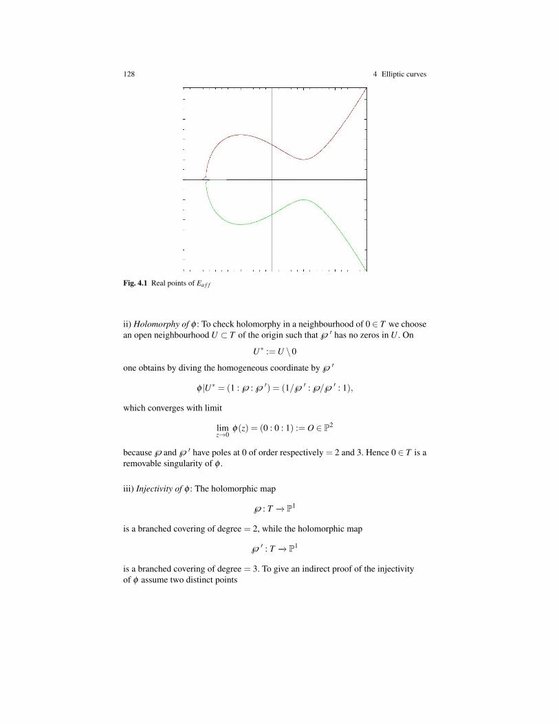
128 4 Elliptic curves
Fig. 4.1 Real points of Ea f f
ii) Holomorphy of φ : To check holomorphy in a neighbourhood of 0 ∈ T we choosean open neighbourhood U ⊂ T of the origin such that ℘ ′ has no zeros in U . On
U∗ :=U \0
one obtains by diving the homogeneous coordinate by ℘ ′
φ |U∗ = (1 :℘ :℘′) = (1/℘ ′ :℘/℘ ′ : 1),
which converges with limit
limz→0
φ(z) = (0 : 0 : 1) := O ∈ P2
because ℘ and ℘ ′ have poles at 0 of order respectively = 2 and 3. Hence 0 ∈ T is aremovable singularity of φ .
iii) Injectivity of φ : The holomorphic map
℘ : T −→ P1
is a branched covering of degree = 2, while the holomorphic map
℘′ : T −→ P1
is a branched covering of degree = 3. To give an indirect proof of the injectivityof φ assume two distinct points

4.1 Embedding tori as plane cubic hypersurfaces 129
z 6= w ∈ T \0
with(℘(z),℘ ′(z)) = (℘(w),℘ ′(w)) ∈ C2.
Then℘(z) =℘(w) implies w =−z
due to Corollary 1.10 and because ℘ is an even function due to Theorem 1.12.Moreover
℘′(z) =℘
′(w) =℘′(−z) =−℘
′(z) implies ℘′(z) = 0.
Lemma 1.13 implies that
z = [ω/2], ω ∈Λ and w =−z ∈ T
are two distinct classes of half-period points of Λ . But ℘ attains at z the value ℘(z)with multiplicity = 2, hence ℘ assumes the value ℘(z) =℘(w) withmultiplicity ≥ 4, a contradiction.
iv) The image of φ : The only non-affine point is
E \Ea f f = O = φ(0).
Consider an affine point(1 : x : y) ∈ E.
The ℘-function is a non-constant holomorphic map
℘ : T −→ P1,
in particular it is surjective: There exists z ∈ T with
℘(z) = x.
The function ℘ is even, therefore also
℘(−z) = x.
Fromy2 = 4x3−g2 · x−g3 = 4℘(z)3−g2 ·℘(z)−g3 =℘
′(z)2
follows:
• Eithery =℘
′(z) and φ(z) = (1 : x : y).
• Ory =−℘
′(z) =℘′(−z) and φ(−z) = (1 : x : y)

130 4 Elliptic curves
v) Smoothness of E:
• A point (x0,y0) ∈C2 is a singular point of Ea f f iff it satisfies the three equations
0 = F(x0,y0) = y20− (4x3
0−Ax0−B), A := g2, B := g3,
∂F∂y
(x0,y0) = 2y0 = 0 and∂F∂x
(x0,y0) =−12x20 +A = 0
Introducing the cubic poynomial
f (x) := 4x3−Ax−B ∈ C[x]
the condition is equivalent to
f (x0) = 0 and f ′(x0) = 0.
The latter condition is equivalent to x0 being a multiple zero of f , i.e. to thevanishing of the discriminant of f
∆ f = A3−27B2.
Proposition 1.19 implies ∆ f 6= 0.
• To prove the non-singularity of E at the point O = (0 : 0 : 1) ∈ P2 we considerthe standard coordinate of P2 around the point O
φ2 : U2 −→ C2, (z0 : z1 : z2) 7→ (u,v) :=
(z0
z2,
z1
z2
).
We haveφ2(E ∩U2) = (u,v) ∈ C2 : f (u,v) = 0
withf (u,v) := u− (4 ·v3−A ·u2 ·v−B ·u3).
Then the partial derivatives are
∂ f∂u
(u,v) = 1− (2 ·A ·u ·v−3 ·B ·u2) and∂ f∂v
(u,v) =−12 ·v2 +A ·u2
hence∇ f (0,0) = (1,0) 6= 0.
The non-singular projective algebraic curve E = φ(T )⊂ P2 is connected, hencea compact Riemann surface with the induced analytic structure as ahypersurface of P2.
vi) Biholomorphy: The map
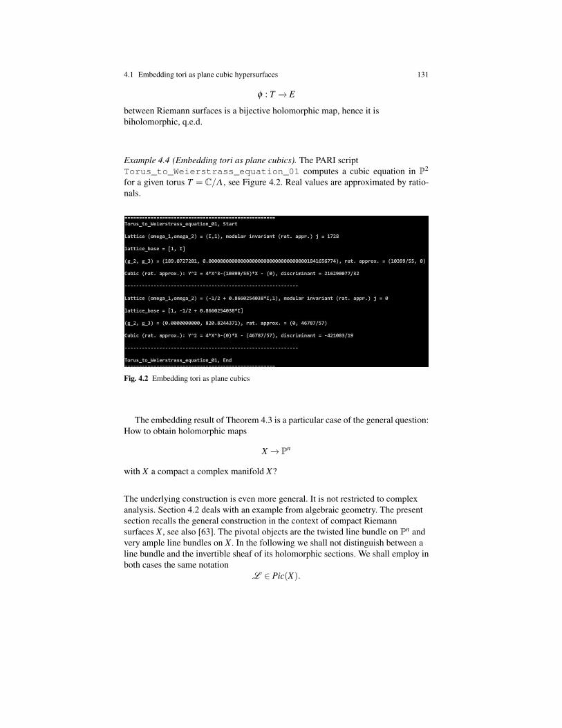
4.1 Embedding tori as plane cubic hypersurfaces 131
φ : T −→ E
between Riemann surfaces is a bijective holomorphic map, hence it isbiholomorphic, q.e.d.
Example 4.4 (Embedding tori as plane cubics). The PARI scriptTorus_to_Weierstrass_equation_01 computes a cubic equation in P2
for a given torus T = C/Λ , see Figure 4.2. Real values are approximated by ratio-nals.
Fig. 4.2 Embedding tori as plane cubics
The embedding result of Theorem 4.3 is a particular case of the general question:How to obtain holomorphic maps
X −→ Pn
with X a compact a complex manifold X?
The underlying construction is even more general. It is not restricted to complexanalysis. Section 4.2 deals with an example from algebraic geometry. The presentsection recalls the general construction in the context of compact Riemannsurfaces X , see also [63]. The pivotal objects are the twisted line bundle on Pn andvery ample line bundles on X . In the following we shall not distinguish between aline bundle and the invertible sheaf of its holomorphic sections. We shall employ inboth cases the same notation
L ∈ Pic(X).

132 4 Elliptic curves
Definition 4.5 (The twisted line bundle on Pn). The twisted line bundle O(1)on Pn is defined with respect to the standard atlas of Pn by the cocycle
g = (gi j) ∈ Z1(U ,O∗)
with
gi j(z0 : ... : zn) :=z j
zi, 0≤ i 6= j ≤ n.
Proposition 4.6 (Sections of O(1)). The sections of O(1) on Pn correspond bijec-tively to the linear polynomials HPol(1)⊂ C[z0, ....,zn], i.e. the map
HPol(1)−→ H0(Pn,O(1)), zk 7→ sk, k = 0, ...,n.
Here sk ∈ H0(Pn,O(1)) is defined with respect to the i-th standard chart by theholomorphic functions
sk,i : Ui −→ C, sk,i(z0 : ... : zn) :=zk
zi
Proof. The map defined above on the standard charts provide a section
sk := (sk,i)i=0,...,n ∈ H0(Pn,O(1))
because
gi j · sk, j =z j
zi·
zk
z j=
zk
zi= sk,i, q.e.d.
Proposition 4.6 generalizes to sections of the tensor powers
O(k) := O(1)⊗k, k ∈ N,
cf. also [63].
In order that a line bundle L on a Riemann surface X defines a holomorphic map
φL : X −→ Pn
to a projective space, the line bundle L has to be globally generated.
Definition 4.7 (Base-point, globally generated line bundle). Consider a Riemannsurface X and a line bundle L on X .

4.1 Embedding tori as plane cubic hypersurfaces 133
1. A point x∈X is a base-point of L if each section σ ∈H0(X ,L ) satisfies σ(x) = 0.Note
σ(x) = 0 ⇐⇒ σx ∈mxLx
with Lx the stalk of L at x ∈ X and
mx ⊂ Ox
the maximal ideal of the stalk Ox of the structure sheaf at x ∈ X .
2. The line bundle is globally generated or base-point-free if it has no base-points,i.e. if for each x ∈ X exists a section σ ∈ H0(X ,L ) such that the germ σx ∈Lxgenerates the stalk Lx as Ox-module. The latter condition is equivalent to σ(x) 6= 0.
Proposition 4.8 (Holomorphic maps to projective spaces). Consider a compactRiemann surface X and a globally generated line bundle L on X. After choosing abasis
(σi)i=0,...,n ∈ H0(X ,L )
the mapφL : X −→ Pn, x 7→ (σ0(x) : ... : σn(x)),
is well-defined, independent from the chosen trivialization of L in a neighbourhoodof x ∈ X, and holomorphic. It induces an isomorphism
φ∗L (O(1))'L
with φ ∗L (O(1)) the pull-back of the twisted line bundle.
Proof. We setφ := φL .
i) Definition: We consider the definition of φ in a suitable open neighbourhood U of x.On U we choose a trivialization to identify the line bundle L with the struc-ture sheaf O . Hence sections from H0(U,L ) become holomorphic functions.Because L is globally generated there is an index j ∈ 0, ...,n with
σ j(x) 6= 0.
Hence the point(σ0(x) : ... : σn(x)) ∈ Pn
is well-defined. It is independent of the choice of the chart and of the isomorphism
L |U ' O|U.
Apparently the map φ is holomorphic on U .

134 4 Elliptic curves
ii) Pullback of the twisted line bundle: For each i = 0, ...,n the sets
Xi := φ−1(Ui) = x ∈ X : (σi)x /∈mxLx
form an open covering (Xi)i=0,...,n of X because L is globally generated.For i = 0, ...,n the canonical morphisms between the rings of local sections
O(1)(Ui)−→ φ∗(L )(Ui) = L (Xi) induced by si|Ui 7→ σi|Xi
define a canonical sheaf morphism on Pn
O(1)−→ φ∗L
The latter corresponds to a sheaf morphism on X
φ∗(O(1))−→L ,
because the two functors φ ∗ and φ∗ are adjoint, see [29, Chap. II, § 5], i.e. there is acanonical group isomorphim
HomOX (φ∗(O(1)),L )' HomOPn (O(1),φ∗L )
The induced morphismφ∗(O(1))−→L
between the two line bundles is an isomorphism because it is an isomorphism onstalks: If for a given i ∈ 0, ...,n
x ∈ Xi ⊂ X and y := φ(x) ∈Ui ⊂ Pn
then according to the definition of the analytic inverse image sheaf
(φ ∗O(1))x = O(1)y⊗OPn ,y OX ,x −→Lx, (si)y⊗1 7→ (σi)x, q.e.d.
Theorem 4.9 provides a geometric criterion for the map provided by a globallygenerated line bundle L to be a closed embedding.
Theorem 4.9 (Projective embedding induced by a line bundle). Consider a com-pact Riemann surface X and a globally generated line bundle L on X. Then theinduced map
φL : X −→ Pn
is a holomorphic closed embedding iff L satisfies both of the following properties:
1. Separating points: For any two distinct points p 6= q ∈ X exists a section
σ ∈ H0(X ,L ) with σ(p) 6= 0 but σ(q) = 0
or vice versa.

4.1 Embedding tori as plane cubic hypersurfaces 135
2. Separating tangent vectors: For all x ∈ X the map
dL ,x : σ ∈ H0(X ,L ) : σx ∈mxLx −→mxLx/m2xLx, σ 7→ [σx],
is surjective.
For the proof of Theorem 4.9 see [63].
Remark 4.10 (Separating points and tangent vectors). We explain the meaning ofthe two statements from Theorem 4.9.
1. Separating points: The homogeneous coordinates of a given point in Pn do notfix the value of the components. But it is determined whether a component iszero or not zero. Therefore for each pair of points p 6= q ∈ X
φL (p) 6= φL (q)
if at least one component of the left-hand side is different from zero while thesame component on the right-hand side is zero.
2. Separating tangent vectors: A holomorphic mapping is an embedding in theneighbourhood of a point x ∈ X if the Jacobi map at x does not vanish. Thelatter condition is equivalent to the fact that at x the push-forward of tangent vec-tors is injective, equivalently the pull-back of cotangent vectors is surjective: Weconsider the isomorphy of Ox-modules - respectively of complex vector spaces -
mxLx/m2xLx ' (mx/m
2x)⊗Ox Lx = T 1
x ⊗Ox Lx
with the cotangent spaceT 1
x :=mx/m2x
of X at x. Then the map
dL ,x : σ ∈ H0(X ,L ) : σx ∈mxLx −→ T 1x ⊗Ox Lx
is induced by the total differential dx of holomorphic functions: A section
σ ∈ H0(X ,L ) with σx ∈mxLx
factorizes in a suitable neighbourhood U of x as
σ = f ·σ1
with a holomorphic function f ∈ O(U) satisfying fx ∈ mx and a holomorphicsection σ1 ∈L (U). Then
dL ,x(σ) = dx f ⊗σ1 ∈ T 1x ⊗Ox Lx

136 4 Elliptic curves
s ∈ H0(Pn,O(1)) : s(y) = 0 T 1Pn,y⊗OPn ,y O(1)y
σ ∈ H0(X ,L ) : σ(x) = 0 T 1X ,x⊗OX ,x Lx
dO(1),y
φ ∗T 1φ ∗
dL ,x
Fig. 4.3 Separating tangent vectors
The commutative diagram from Figure 4.3 with
y := φ(x)
and surjective mapsdO(1),y and φ
∗
shows: The pull-back φ ∗T 1 is surjective if and only if dL ,x is surjective.
Definition 4.11 (Very ample line bundle). A globally generated line bundle L ona compact Riemann surface X is very ample if the induced map
φL : X −→ Pn
is an embedding.
A globally generated line bundle L on X has enough sections to define a holo-morphic map
φL : X −→ Pn.
If L is very ample then there are enough sections that φL is even an embedding.Due to the compactness of X its image under an embedding is always closed.
Notation 4.12. For a line bundle L on a Riemann surface X and a divisor D ∈ Div(X)we denote by
LD := L ⊗O OD
the sheaf of meromorphic sections of L which are multiples of the divisor −D. Thesheaf LD is isomorphic to a line bundle.
Consider a line bundle L on a compact Riemann surface X . Theorem 4.13 statesa numerical criterion for the dimension of the vector spaces

4.1 Embedding tori as plane cubic hypersurfaces 137
H0(X ,LD), D ∈ Div(X),
which ensures that the mapφL : X −→ Pn
is well-defined and a closed embedding. This criterion is very helpful in the applica-tions because the dimension on the vector spaces in question can often be computedby using the theorem of Riemann-Roch in combination with Serre duality.
Theorem 4.13 (Very-ampleness criterion). Consider a compact Riemann surface X.For a line bundle L on X are equivalent:
• The line bundle L is very ample.
• For any two not necessarily distinct points p, q ∈ X the corresponding point di-visors
P := 1 · p, Q := 1 ·q ∈ Div(X)
satisfydim H0(X ,L−(P+Q)) = dim H0(X ,L )−2.
Proof. i) Assume the validity of the dimension formula: The formula implies for anytwo point divisors P, Q ∈ Div(X)
H0(X ,L−(P+Q))( H0(X ,L−P)( H0(X ,L )
and each proper inclusion has codimension = 1 because it is defined by a singlelinear equation.
• The equationh0(X ,L−P) = h0(X ,L )−1.
states that the kernel of the evaluation
H0(X ,L )−→Lp/mpLp ' C, σ 7→ [σp],
has codimension = 1. Hence p is not a base-point of L . As a consequence, theline bundle L is globally generated and
φL : X −→ Pn
is well-defined.
• The equationH0(X ,L−(P+Q))( H0(X ,L−P)
implies that for any pair of distinct points p, q ∈ X there exists a section
σ ∈ H0(X ,L−P)\H0(X ,L−(P+Q))
138 4 Elliptic curves
i.e. satisfyingσ(p) = 0 but σ(q) 6= 0.
Hence the sheaf L separates points.
• The dimension formula shows for any point p ∈ X with point divisor P ∈Div(X)
H0(X ,L−2P)( H0(X ,L−P)
has codimension = 1. Hence there exists a section
σ ∈ H0(X ,L−P)\H0(X ,L−2P)
which implies the surjectivity of the composition of the canonical maps
H0(X ,L−P)−→mX ,pLp −→mX ,pLp/m2X ,pLp
due todimC(mX ,p/m
2X ,p) = 1.
Therefore L separates tangent vectors.
ii) Assume L very ample: Theorem 4.9 implies that L separates points andtangent vectors. Separating points implies for all point divisors P 6= Q ∈ Div(X)
dim H0(X ,L−(P+Q)) = dim H0(X ,L )−2.
Separating tangent vectors implies for each point divisor P ∈ Div(X)
dim H0(X ,L−2P) = dim H0(X ,L )−2, q.e.d.
Remark 4.14 (Projective embedding of compact Riemann surfaces). As a conse-quence of the very-ampleness criterion from Theorem 4.13 one can prove: Eachcompact Riemann surface X embeds holomorphically into a projective space.
1. If g(X) ≥ 2 then the tri-canonical line bundle Ω⊗3 ∈ Pic(X) is very ample,see [63].
2. For a complex torus X = C/Λ holds Ω ' O , hence
g(X) := dim H0(X ,Ω) = 1
Consider the divisorD := 3 ·0 ∈ Div(X)
with the point 0 ∈ X being the origin. Then the line bundle

4.2 Elliptic curves over subfields of C 139
L := OD ∈ Pic(X)
is very ample according to Theorem 4.13: As a consequence of Ω ' O , for twopoint divisors
P = 1 · p, Q = 1 ·q ∈ Div(X)
holdsdim H1(X ,L−(P+Q)) = dim H0(X ,O−D+(P+Q)) = 0
becausedeg (−D+(P+Q)) =−3+2 =−1 < 0
Hence
dim H0 (X ,L−(P+Q)
)= 1−g(X)+deg L −2 = dim H0(X ,L )−2
The Riemann-Roch theorem implies
dim H0(X ,L ) = dim H0(X ,OD) = deg D = 3
Apparently, a basis of H0(X ,OD) is the family of linearly independent elements
(1,℘,℘ ′),
which gives a second proof for the embedding from Theorem 4.3.
4.2 Elliptic curves over subfields of C
Complex Analysis of several variables or Complex Analytic Geometry on one hand,and on the other hand Algebraic Geometry are mathematical theories with manyconcepts in common and also several concepts in parallel. We compile the followingGAGA-dictionary (Geometrie Algebrique et Geometrie Analytique).
Proposition 4.15 (Dictionary: Complex Analytic Geometry - Algebraic Geom-etry).
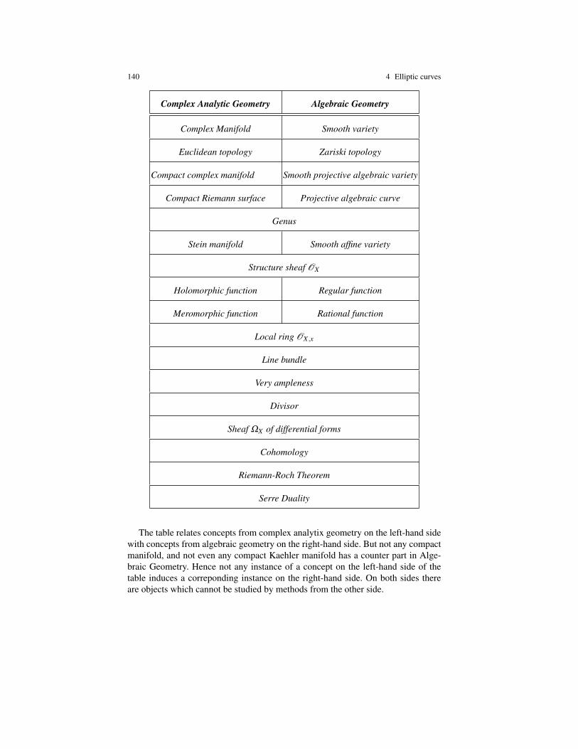
140 4 Elliptic curves
Complex Analytic Geometry Algebraic Geometry
Complex Manifold Smooth variety
Euclidean topology Zariski topology
Compact complex manifold Smooth projective algebraic variety
Compact Riemann surface Projective algebraic curve
Genus
Stein manifold Smooth affine variety
Structure sheaf OX
Holomorphic function Regular function
Meromorphic function Rational function
Local ring OX ,x
Line bundle
Very ampleness
Divisor
Sheaf ΩX of differential forms
Cohomology
Riemann-Roch Theorem
Serre Duality
The table relates concepts from complex analytix geometry on the left-hand sidewith concepts from algebraic geometry on the right-hand side. But not any compactmanifold, and not even any compact Kaehler manifold has a counter part in Alge-braic Geometry. Hence not any instance of a concept on the left-hand side of thetable induces a correponding instance on the right-hand side. On both sides thereare objects which cannot be studied by methods from the other side.

4.2 Elliptic curves over subfields of C 141
In Algebraic Geometry a variety is assumed to be irreducible. Irreducibility cor-responds to connectedness in the case of manifolds. If one skips the requirement ofsmoothness one obtains the irreducible reduced complex space as the analogue of avariety.
Remark 4.16 recalls varieties as the basic objects of classical algebraic geometry.Varieties are irreducible by definition, hence they are defined by prime ideals. Butdifferent from manifolds varieties may have singularities. Hence varieties are theanalogue of reduced and irreducible complex spaces. We distinguish between theirfield k of definition and the algebraic closure k where the points of the variety havetheir coordinates. As a topological space varieties will be equipped with the Zariskitopology.
Recall that a field k is perfect if each irreducible polynomial with coefficientsfrom k is separable, i.e has pairwise distinct roots in an algebraic closure k. Allfields in the present section will be assumed perfect. The relevant examples of per-fect fields are the fields k of characteristic = 0 or the finite fields k = Fp of primecharacteristic = p.
Remark 4.16 (Algebraic variety with structure sheaf). Consider a perfect field k anddenote by k the algebraic closure of k.
1. Variety: An affine algebraic variety X is the zero set
X =V (a)⊂ An(k) = kn
of a prime ideal a⊂ k[X1, ...,Xn], i.e.
X := x ∈ An(k) : f (x) = 0 for all f ∈ a.
The ringR := k[X1, ...,Xn]/a
is the affine coordinate ring of X .
If a can be generated by polynomials from k[X1, ...,Xn], then X is defined over k,denoted X/k. The smallest subfield of k with this property is named the field ofdefinition of X .
2. A projective algebraic variety X is the zero set
X =V (a)⊂ Pn(k)
of a prime ideala⊂ k[X0, ...,Xn],

142 4 Elliptic curves
generated by homogeneous polynomials, i.e.
X := (x = (x0 : ... : xn) ∈ Pn(k) : f (x) = 0 for all homogeneous f ∈ a.
3. Zariski topology: Closed sets of An(k) are the affine algebraic subvarieties andtheir finite unions. The Zariski topology on an affine algebraic variety X ⊂An(k)is the subspace topology induced from the Zariski topology of An(k). A basis ofthe Zariski topology of X are the sets
Dh := x ∈ X : h(x) 6= 0, h ∈ R.
Closed sets of Pn(k) are the projective algebraic subvarieties. The Zariski topol-ogy on a projective algebraic variety X ⊂ Pn(k) is the subspace topology inducedfrom the Zariski topology of Pn(k).
Non-empty open subsets of an irreducible space are irreducible itself, and arealso dense.
4. Structure sheaf and sheaf of rational functions: Consider an affine algebraic va-riety X and an open set U ⊂ X . A function
f : U → k
is regular if it has locally the form
f =gh
with g,h ∈ R, h locally without zeros in X .
Note that the quotient representation of f is only required to hold locally. Thesheaf OX of regular functions on an affine algebraic variety X is the contravariantfunctor
U 7→ OX (U) := f : U → k| f regular , U ⊂ X open,
with the restriction of functions. The sheaf OX is named the structure sheaf of X .Sections over a basis open set Dh ⊂ X form the ring
O(Dh) = Rh := g/hn : g ∈ R, n ∈ N
Because the ideala⊂ k[X1, ...,Xn]
is prime, the quotient R and all rings
OX (U), U ⊂ X open,
are integral domains. The sheaf MX of rational functions on X is the sheafifica-tion of the presheaf
U 7→ Q(OX (U)), U ⊂ X open,

4.2 Elliptic curves over subfields of C 143
with Q(OX (U)) the quotient field of the integral domain OX (U). Sections of MX (U)are locally quotients
g/h, g, h ∈ R, h 6= 0.
For a non-empty open set U ⊂ X holds
M (U) = Q(R) =: k(X),
independent from U . The field Q(R) is named the function field k(X) of X . Thesheaf
M ∗ ⊂M
is the multiplicative subsheaf of non-zero rational functions.
The definitions carry over to projective algebraic varieties, beaucse the latterhave an atlas of affine algebraic varieties.
5. Non-singularity: Consider an algebraic variety X and a point x ∈ X . The localring OX ,x at x ∈ X is the ring of germs of regular functions defined in a neigh-bourhood of x ∈ X . Its dimension defines the dimension of X at x ∈ X .
The variety X is non-singular or smooth at x ∈ X if OX ,x is a regular local ring,i.e. if
dim OX ,x = dimκ(x) (mx/mx2) (Dimension equals cotangent dimension).
Hereκ(x) := OX ,x/mx
denotes the residue field of X at x.
6. Curve over k: A projective algebraic curve C/k is a 1-dimensional, non-singularprojective algebraic variety defined over the field k. If
C ⊂ P2(k)
then C/k is a plane projective algebraic curve. Its genus is defined as
g(C) = dimk H0(C,Ω),
the dimension of the k-vector space of regular differential forms.
7. Affine schemes: From a modern viewpoint the primary property of a variety is notthe point set
X ⊂ An(k),
the primary object is the ideal
a⊂ k[X1, ...,Xn]

144 4 Elliptic curves
with minimal field of definition k, or its quotient, the ring
R := k[X1, ...,Xn]/a
Due to Grothendieck’s reformulation of algebraic geometry, the basic concept isfor arbitrary rings R the affine scheme
(X := Spec R,OX )
Here Spec R is a topological space with points the prime ideals of R. The structuresheaf OX has as stalks the localizations
Rp, p⊂ R prime ideal.
We have included the requirement of non-singularity into our definition of aprojective algebraic curve because all curves under consideration will be assumedsmooth if not stated otherwise. Note that any plane projective algebraic curve isdefined by a single homogeneous polynomial. Its degree is the degree of C/k.
Remark 4.16 for X/k involves two fields:
• First, the field of definition k is not necessarily algebraically closed. It is theminimal field where the coefficients of a set of generators of I(X) may be takenfrom.
• Secondly, the algebraically closed field k, used to visualize K/k as a point set Xfrom a geometrical view point. Also the condition on smoothness refers to k.
But the set X ⊂ An(k) respectively X ⊂ Pn(k) is not the only point set attachedto K/k. Definition 4.17 introduces point sets X(K) attached to all intermediatefields k ⊂ K ⊂ k.
Definition 4.17 (K-valued point pf X/k). Consider a projective algebraic variety X/kwith
X ⊂ Pn(k).
Then for any fieldk ⊂ K
the set of K-valued points of X is defined as
X(K) := X ∩Pn(K) =

4.2 Elliptic curves over subfields of C 145
= x = (x0 : ... : xn) ∈ Pn(k) : x ∈ X and xi ∈ K f or all i = 0, ...,n.
Remark 4.18 (GAGA).
1. Chow’s theorem: Historically, the first GAGA-result is Chow’s theorem: Anyprojective complex analytic manifold X ⊂Pn is the variety of homogeneous poly-nomials, i.e. if X ⊂ Pn is locally defined as the zero set of holomorphic functions,then X can be globally defined by homogenous polynomials.
2. Analytification of schemes: To formalize the analogy between complex analyticgeometry and complex algebraic geometry Grothendieck uses the language ofcategory theory. On one hand, let AnC denote the category of complex spaces andholomorphic maps. On the other hand, let AlC denote the category of schemesof finite type defined over C and regular maps. The first step attaches to aschema X ∈ AlC a distinguished complex analytic space Xan ∈ AnC. The latteris obtained via the functor:
Φ : AnC −→ Ens
attaching to a complex analytic space Y the set
Φ(Y ) := HomC(Y,X)
of morphisms of ringed spaces. The functor Φ can be represented by a universalobject (Xan,φ), named the analytification of X . The pair comprises a complexanalytic space Xan and a morphism
φ : Xan −→ X ,
see [46]. As a consequence: For a given complex analytic space Y each morphism
f : Y −→ X
of ringed spaces induces a unique holomorphic map
f an : Y −→ Xan,
such that the following diagram commutes
Y
Xan X
f an
φ
f
The analytification φ : Xan −→ X from the analytification defines for each x ∈ Xan
a pull-back

146 4 Elliptic curves
φx : OX ,φ(x) −→ OXan,x
which allows to compare the local ring of regular functions on X and the localring of holomorphic functions on Xan. As a consequence one obtains compari-son theorems between the algebraic properties of the local rings of the structuresheaves of X and Xan, see [46, Chap. 2].
In addition, any morphism f : X →Y in AnC induces a unique holomorphic map
f an : Xan −→ Y an
such that the following diagram commutes
Xan X
Y an Y
φX
φY
f an f
Again, one obtains comparison theorems between the algebraic properties of themorphisms
f : X → Y and f an : Xan −→ Y an,
see [46, Chap. 3].
3. Coherent sheaves and proper maps: The morphism
φ : X −→ Xan
from the analytification of X defines the functor analytical inverse image as thepull-back of module sheaves over the structure sheaf:
φ∗ : Shea f
OX−→ Shea f
OXan, F 7→ φ
∗F
andf : F −→ G , 7→ φ
∗ f : φ∗F −→ φ
∗G .
The stalk at a point x ∈ Xan of the inverse image sheaf is easy to calculate
(φ ∗F )x = Fφ(x)⊗OX ,φ(x)OXan,x
Serre investigated in his GAGA-paper [49] for a projective schema X ∈ AlC anda coherent OX -module the relation between the cohomology in the algebraic andthe analytic category. Subsequently his results have been generalized to the rela-tive case: For a proper morphism
f : X −→ Y

4.2 Elliptic curves over subfields of C 147
in AlC and a coherent OX -module sheaf F the canonical morphisms in AnC be-tween the corresponding direct image sheaves
(R j f∗F )an '−→ R j f an∗ (F an), j ∈ N,
are isomorphisms, see [46, Chap. 4].
The literal analogue of divisors on compact Riemann surfaces are divisors ona projective algebraic curve C/k. A priori, these divisors refer to the points of thecurve C ⊂ Pn(k) with coordinates in k. In a second step we will consider thosedivisors which are defined over k.
Definition 4.19 (Divisors on projective algebraic curves). Consider a projectivealgebraic curve C/k with C ⊂ Pn(k).
1. A divisor on C/k is formal sum
D = ∑x∈C
nx · x
with integers nx ∈ Z satisfying nx = 0 for all but finitely many indices. For apoint p ∈C the corresponding point divisor is denoted
P := 1 · p
Each divisor D ∈ Div(C) has a well-defined degree
deg D := ∑x∈C
nx ∈ Z
The additive group of divisors on C/k is denoted Div(C), its subgroup Div0(C)⊂ Div(C)contains the classes of divisors of degree = 0.
2. A divisor D ∈ Div(C) is a principal divisor if D = 0 or
D = div f
for a rational function f ∈ k(C). Two divisors D1,D2 ∈ Div(C) are equivalent,annotated
D1 ∼ D2,
if their difference is a principal divisor. The divisor of a rational function f ∈ k∗
has degreedeg (div f ) = 0.
Denote byPrin(C)⊂ Div0(C)

148 4 Elliptic curves
the subgroup of principal divisors. The quotient
Cl(C) := Div(C)/Prin(C)
is named the divisor class group of C. Its subgroup
Cl0(C) := Div0(C)/Prin(C)⊂Cl(C)
is the class group of degree zero divisors.
3. A divisorD = ∑
x∈Cnx · x ∈ Div(C)
is defined over k if it is invariant under the action of the Galois group Gk/k, i.e. iffor all σ ∈ Gk/k
D = Dσ := ∑x∈C
nx · xσ ∈ Div(C)
4. For a divisor D ∈ Div(C) we denote by OD the sheaf of multiples of −D, i.e.
OD(U) := f ∈M ∗(U) : div f ≥−D|U∪0, U ⊂ X open.
For projective-algebraic curves C/k the theorems of Riemann-Roch, Serre dual-ity, the very-ampleness criterion from Theorem 4.13 and the dimension formula
dim H0(C,O) = 1
hold literally in the same form as on compact Riemann surfaces. Also the canonicaldivisor K ∈ Div(C) has degree
deg K = 2g(C)−2.
Hence we will apply these results also in the context of algebraic geoemtery withoutfurther mentioning.
Definition 4.20 (Elliptic curve over k). An elliptic curve defined over k is apair (E,O) with
• a projective algebraic curve E/k of genus g = 1
• and a k-valued point O ∈ E
Note. In Definition 4.20 “O” denotes the upper-case letter O, not the digit 0. Wedenote by
O∞ := 1 ·O ∈ Div(E)

4.2 Elliptic curves over subfields of C 149
the distinguished point divisor. It is defined over k.
If the base field k and the k-valued point O are not relevant for the context, we willoften denote an elliptic curve just by E.
Note that there exist smooth projective algebraic curves C/Q of genus g = 1without rational points, i.e. with C(Q) = /0. An example is the Selmercurve C ∈ P2(C) defined by the homogeneous cubic equation
3X3 +4Y 3 +5Z3 = 0.
The fact g = 1 for an elliptic curve E allows a simple application of the Riemann-Roch theorem to compute the vector spaces of multiples of a divisor on E.
Lemma 4.21 (Divisors on an elliptic curve). Consider an elliptic curve E and adivisor D ∈ Div(E). Then
dim H0(E,OD) =
0 if deg D < 00 if deg D = 0, D not principal1 if deg D = 0, D principaldeg D if deg D > 0
Proof. The Riemann-Roch theorem together with Serre duality imply for anydivisor D ∈ Div(E)
dim H0(E,OD)−dim H1(E,OD) = dim H0(E,OD)−dim H0(E,O−D+K) =
= 1−g+deg D = deg D
Because an elliptic curve E has genus g = 1, its canonical divisor has degree
deg K = 2g−2 = 0.
As a consequence
deg (−D+K) = deg (−D) =−deg D
i) Case deg D 6= 0: If deg D > 0 then deg (−D)< 0. As a consequence
dim H0(E,OD) =
deg D if deg D > 00 if deg D < 0
ii) Case deg D = 0: We consider the sheaf OD as a line bundle. Then
D principal ⇐⇒ OD 'O

150 4 Elliptic curves
On one hand, D principal implies
H0(E,OD) = dim H0(E,O) = 1
On the other hand, for non-principal D the line bundle OD is not trivial. Hence eachregular section of s ∈ H0(E,OD) has a zero. If s 6= 0, then deg D = 0 implies that shas also at least a pole, contradicting the regularity of s. Therefore s = 0, q.e.d.
The following Lemma 4.22 will be used in the proof of Theorem 4.23. It indi-cates why the existence of a k-valued point is requested for an elliptic curve definedover k.
Lemma 4.22 (Divisors defined over a subfield). Consider a projective algebraiccurve C/k and a divisor
D = ∑x∈X
nx · x ∈ Div(C)
which is defined over k. Then the finite dimensional k-vector space
H0(C,OD) = f ∈ k∗(C) : div f ≥−D∪0
has a basis of rational functions from k(C), more precisely
H0(C,OD) = k⊗k f ∈ k∗(C) : div f ≥−D∪0
For the proof see [56, II, Prop. 5.8].
Elliptic curves are by definition subvarieties of a projective space Pn(k). Theorem 4.23proves that they are even plane curves, i.e. that they embed as hypersurfacesinto P2(k).
Theorem 4.23 (Elliptic curves are plane cubics). For an elliptic curve (E/k,O)exist two rational functions x,y ∈ k(E) with poles only at O such that the map
φ : E→ P2(k), p 7→
(1 : x(p) : y(p)) p 6= O(0 : 0 : 1) p = O
induces an isomorphism onto the plane cubic C ⊂ P2(k), which is defined by ahomogeneous polynomial Fhom ∈ k[X0,X1,X2] of the form
Fhom(X0,X1,X2) = X0X22 +a1X0X1X2 +a3X2
0 X2− (X31 +a2X0X2
1 +a4X20 X1 +a6X3
0 )
with five suitable constants ai ∈ k, i = 1,2,3,4,6. In particular, C is defined over kand non-singular.
Proof. We construct a very ample line bundle L = OD on E and define φ := φL .Therefore consider the divisor

4.2 Elliptic curves over subfields of C 151
D := 3 ·O∞ ∈ Div(E).
The line bundleL := OD ∈ Pic(E)
satisfies the very ampleness criterion from Theorem 4.13: The proof follows fromthe dimension formula in Lemma 4.21 because for all points p,q ∈ E
dim H0(E,OD−P) = dim H0(E,OD)−1
anddim H0(E,OD−(P+Q)) = dim H0(E,OD)−2.
For n≥ 0
H0(E,On·O∞)) = f ∈ k∗(E) : f has at most a pole at O of order = n∪0
and the dimension formula implies the proper inclusion
H0(E,O3·O∞)) H0(E,O2·O∞
)) H0(E,OO∞)' H0(E,O) = C.
Hence a basis (1,x,y) of
H0(E,L ) = H0(E,O3·O∞)
exists with
• y ∈ H0(E,O3·O∞)⊂ k(E) has a pole of order = 3 at O and no other pole,
• x ∈ H0(E,O2·O∞)⊂ k(E) has a pole of order = 2 at O and no other pole,
• 1 ∈ H0(E,O) = H0(E,O1·O∞)⊂ k(E) has no poles.
By assumption O ∈ E(k). Therefore the divisor D is defined over k. According toLemma 4.22 we may choose even x,y ∈ k(E). With respect to the basis (1,x,y) theline bundle L defines the closed embedding
φ := φL : E→ P2(k), p 7→ (1 : x(p) : y(p)),
onto a curve C/k in P2(k). The family
(1, x, y, x2, xy, x3, y2)
of seven rational functions from the 6-dimensional vector space H0(E,O6·O∞) is
linearly dependent. Therefore the functions satisfy a linear relation with coefficientsfrom k. Among them the two functions x3 and y2 are the only ones having a poleat O ∈ E of order = 6. Hence their coefficients in the linear relation are not zero.After division we may assume that their coefficients are =±1 and
y2 +a1xy+a3y = x3 +a2x2 +a4x+a6
152 4 Elliptic curves
with coefficients ai ∈ k. This relation defines the inhomogeneous polynomial
F(X ,Y ) := Y 2 +a1XY +a3Y − (X3 +a2X2 +a4X +a6) ∈ k[X ,Y ]
and its homogenization, the polynomial Fhom ∈ k[X0,X1,X2] with
Fhom(X0,X1,X2) := X0X21 +a1X0X1X2+a3X2X2
0 −(X31 +a2X2
1 X0+a4X1X20 +a6X3
0 ).
The inhomogeneous variables (X ,Y ) relate to the homogeneous variables (X0,X1,X2)according to
X =X1
X0and Y =
X2
X0.
The curve φ(E) is a subvariety of the 1-dimensional cubic hypersurface
C :=V (Fhom)⊂ (x0 : x1 : x2) ∈ P2(k) : Fhom(x0,x1,x2) = 0.
The cubic C intersects the line at infinity
P1(k)' (x0 : x1 : x2) ∈ P2(k) : x0 = 0
in the single point (0 : 0 : 1) with multiplicity = 3. Its affine part is the affine varietyof the polynomial F(X ,Y ) ∈ k[X ,Y ]
Caff = (x0 : x1 : x2) ∈ P2(k) : Fhom((x0 : x1 : x2)) = 0 and x0 6= 0=
= (x,y) ∈ A2(k) : F(x,y) = 0=V (F).
The polynomial F ∈ k[X ][Y ], considered as polynomial in Y with coefficients fromthe ring k[X ], is irreducible: It does not split as
F(X ,Y ) = (Y +b1)(Y +b2)
with polynomials b1,b2 ∈ k[X ]. Therefore Caff and also C are irreducible. Hence thenon-constant regular map
φ : E→C
is surjective, cf. [29, Chap. II, Prop. 6.8], an analogue of the theorem about non-constant proper holomorphic maps between Riemann surfaces. As a consequence
φ(E) =C and E 'C over k
and C is non-singular, q.e.d.
In the following we will identify an abstract elliptic curve (E/k,O) with the planecubic from Theorem 4.23. We say that (E/k,O), more precisely its affine part, isdefined over k by the Weierstrass equation F(X ,Y ) = 0.

4.2 Elliptic curves over subfields of C 153
Definition 4.24 (Weierstrass polynomial and Weierstrass equation, its discrim-inant and j-invariant). A Weierstrass polynomial over a field k is a cubic poyno-mial
F(X ,Y ) = Y 2 +a1XY +a3Y − (X3 +a2X2 +a4X +a6) ∈ k[X ,Y ]
with coefficientsa1, a2, a3, a4, a6 ∈ k.
1. The equationF(X ,Y ) = 0,
i.e.Y 2 +a1XY +a3Y = X3 +a2X2 +a4X +a6
is named the Weierstrass equation over k defined by F .
2. The discriminant of F is
∆F :=−b22b8−8b3
4−27b26 +9b2b4b6
withb2 := a2
1 +4a2, b4 := 2a4 +a1a3, b6 := a23 +4a6
andb8 := a2
1a6 +4a2a6−a1a3a4 +a2a23−a2
4.
3. The j-invariant of F is
jF :=c3
4
∆F, c4 := b2
2−24bb.
Starting from an elliptic curve over a field k the resulting Weierstrass polynomialis not unique. There exist coordinate transformations defined over k which transforma Weierstrass polynomial over k to a different form, in particular to a more simpleform.
Proposition 4.25 (Weierstrass equation in short form, discriminant and j-invariant).Consider a Weierstrass polynomial
F(X ,Y ) = Y 2 +a1XY +a3Y − (X3 +a2X2 +a4X +a6) ∈ k[X ,Y ]
1. Short form: If char k 6= 2,3 then there exists a linear coordinate change(XY
)7→(
X ′
Y ′
)=
(u2 ·X + r
u3 ·Y + s ·u2 ·X + t
)with constants
r,s, t ∈ k,u ∈ k∗
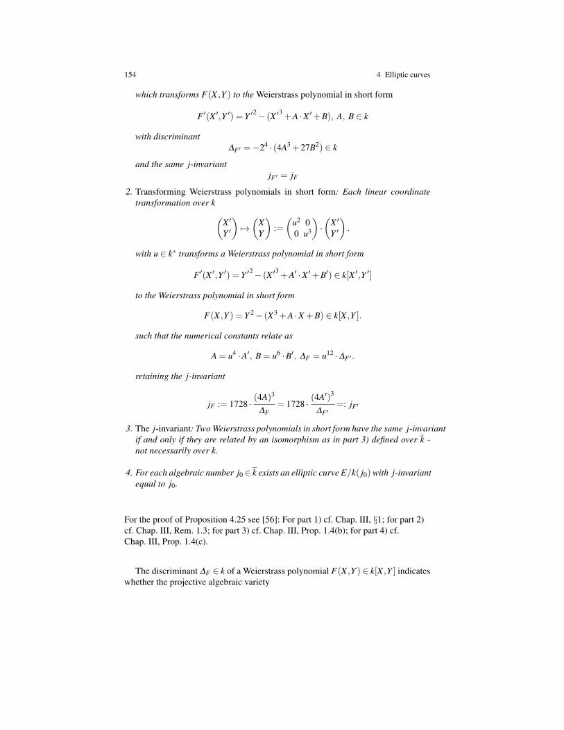
154 4 Elliptic curves
which transforms F(X ,Y ) to the Weierstrass polynomial in short form
F ′(X ′,Y ′) = Y ′2− (X ′3 +A ·X ′+B), A, B ∈ k
with discriminant∆F ′ =−24 · (4A3 +27B2) ∈ k
and the same j-invariantjF ′ = jF
2. Transforming Weierstrass polynomials in short form: Each linear coordinatetransformation over k(
X ′
Y ′
)7→(
XY
):=(
u2 00 u3
)·(
X ′
Y ′
).
with u ∈ k∗ transforms a Weierstrass polynomial in short form
F ′(X ′,Y ′) = Y ′2− (X ′3 +A′ ·X ′+B′) ∈ k[X ′,Y ′]
to the Weierstrass polynomial in short form
F(X ,Y ) = Y 2− (X3 +A ·X +B) ∈ k[X ,Y ].
such that the numerical constants relate as
A = u4 ·A′, B = u6 ·B′, ∆F = u12 ·∆F ′ .
retaining the j-invariant
jF := 1728 ·(4A)3
∆F= 1728 ·
(4A′)3
∆F ′=: jF ′
3. The j-invariant: Two Weierstrass polynomials in short form have the same j-invariantif and only if they are related by an isomorphism as in part 3) defined over k -not necessarily over k.
4. For each algebraic number j0 ∈ k exists an elliptic curve E/k( j0) with j-invariantequal to j0.
For the proof of Proposition 4.25 see [56]: For part 1) cf. Chap. III, §1; for part 2)cf. Chap. III, Rem. 1.3; for part 3) cf. Chap. III, Prop. 1.4(b); for part 4) cf.Chap. III, Prop. 1.4(c).
The discriminant ∆F ∈ k of a Weierstrass polynomial F(X ,Y ) ∈ k[X ,Y ] indicateswhether the projective algebraic variety

4.2 Elliptic curves over subfields of C 155
C =V (Fhom)⊂ P2(k)
is non-singular or not. If ∆F 6= 0 then (C/k,(0 : 0 : 1)) is non-singular, i.e. an ellipticcurve.
Proposition 4.26 (Singularities of cubics). Assume char k 6= 2,3 and consider aplane cubic curve
C :=V (Fhom) =⊂ P2(k)
defined by the homogenization of a Weierstrass polynomial in short form
F(X ,Y ) = Y 2− (X3 +AX +B) ∈ k[X ,Y ]
with A, B ∈ k and discriminant
∆F =−16 · (4A3 +27B2).
The curve C has at most one singular point. The curve
• is non-singular iff ∆F 6= 0
• has a node iff ∆F = 0 and A 6= 0
• has a cusp iff ∆F = A = 0.
For a proof of Proposition 4.26 see [56, Chap. III, Prop. 1.4].
Remark 4.27 (Cubic projective-algebraic curves and elliptic curves). The adjunc-tion formula for non-singular hypersurfaces implies: Any projective algebraic cu-bic curve C ⊂ P2 has genus = 1. Hence C/k is an elliptic curve if C has at leastone k-valued point, see [29, Chap. V, Example. 1.5.1].
Theorem 4.28 is the converse of Theorem 4.3. it shows that the complex points ofan elliptic curve, defined over a subfield of C, can be parametrized by theWeierstrass function ℘ and its derivative ℘ ′ of a suitable torus. The proof relies onthe result of Theorem 4.23 that elliptic curves are plane cubics which satisfy aWeierstrass equation.A very coarse analogue of the uniformization is the parametrization of the points ofthe unit circle by the values of the exponential function e2πi·t on the parameterinterval [0,1].
Theorem 4.28 (Uniformization of elliptic curves E/C by tori). For any ellipticcurve E defined over C exists a torus T = C/Λ and a biholomorphic map
Φ : T '−→ E(C).
Here E(C) ⊂ Pn(C) is provided with the induced Euclidean topology and analyticstructure from the complex manifold Pn(C) = Pn.

156 4 Elliptic curves
Proof. Due to Theorem 4.23 we may assume that E is defined as a plane curve,defined by the homogenization of a Weierstrass polynomial in short form
F(X ,Y ′) := Y ′2− (X3 +a4 ·X +a6) ∈ C[X ,Y ′].
The substitutionY ′ = (1/2) ·Y
shows that E can also be defined by the Weierstrass polynomial
F(X ,Y ) = Y 2− (4 ·X3−A ·X−B)
with suitable constants A, B ∈ C and discriminant
∆F = A3−27 ·B3
due to Proposition 4.26. We search for a lattice
Λ = Zω1 +Zω2 ⊂ C
with lattice constants GΛ ,4 and GΛ ,6 satisfiying
A = 60 ·GΛ , 4 and B = 140 ·GΛ , 6.
The restriction of the modular invariant
j|H : H→ C, j(τ) := 1728 ·g3
2(τ)
g32(τ)−27g2
3(τ),
is surjective according to Corollary 3.16. Hence a number τ ∈H exists with
j(τ) = 1728 ·A3
∆F.
If g2(τ) = 0 then τ = ρ according to Corollary 3.20. We choose
Λ := Λρ .
Similarly, if g3(τ) = 0 then τ = i, and we choose
Λ := Λi.
Otherwise, the two equations
j(τ) = 1728 ·g3
2(τ)
g32(τ)−27g2
3(τ)= 1728 ·
A3
∆F
and∆F = A3−27B2

4.2 Elliptic curves over subfields of C 157
implyg3
2(τ)
g32(τ)−27g2
3(τ)=
A3
A3−27 ·B2.
Clearing the denominators by crosswise multiplication implies(A
g2(τ)
)3
=
(B
g3(τ)
)2
We choose ω1 ∈ C with
Ag2(τ)
=
(1
ω1
)4
andB
g3(τ)=
(1
ω1
)6
.
This choice is possible because we may replace ω1 by iω1. In addition, we set
ω2 := τ ·ω1, i.e. τ = ω2/ω1.
Then (ω1,ω2) is a positively oriented basis of the lattice
Λ := Zω1 +Zω2.
Its lattice constants are
GΛ ,4 =
(1
ω1
)4
·G4(τ) =
(1
ω1
)4
· (1/60) ·g2(τ) = (1/60) ·A
and similarlyGΛ ,6 = (1/140) ·B,
i.e.A = gΛ ,2 and B = gΛ ,3.
The mapφ : C/Λ −→ P2
from Theorem 4.3 maps the torus C/Λ biholomorphically to the cubic hypersurfacewith Weierstrass polynomial
F(X ,Y ) = Y 2− (4 ·X3−gΛ ,2 ·X−gΛ ,3) = Y 2− (4 ·X3−A ·X−B), q.e.d.
Example 4.29 (Elliptic curves and cubics with a singularity). The following Figures 4.5 - 4.8show some elliptic curves.
While Figure 4.9 and Figure 4.10 show the singular cubics node and the Neilparabola. They have a single singularity, namely at the origin respectively a nodeand a cusp. The corresponding table from Figure 4.4 shows the invariants. The roleof the conductor will be explained in Definition 4.40 later.

158 4 Elliptic curves
For the computation and the plots see the PARI files Elliptic_curve_02and Elliptic_curve_plot_06.
Figure Weierstrass equation j-invariant discriminant conductor
Elliptic curve
4.5 Y 2 = X3−3X +3 −28 ·33/5 −24 ·33 ·5 23 ·33 ·5
4.6 Y 2 = X3 +X 1728 −26 26
4.7 Y 2 = X3−X 1728 26 25
4.8 Y 2 = X3 +3 0 −24 ·35 24 ·35
Y 2 = X3−X−14 −25 ·33/661 −27 ·661 27 ·661
Y 2 +5XY +Y = X3 53 ·1013/(2 ·72) 2 ·72 2 ·7
Singular cubic
4.9 Y 2 = X3 +X2 − 0 −
4.10 Y 2 = X3 − 0 −
Fig. 4.4 Numerical values of some cubic curves
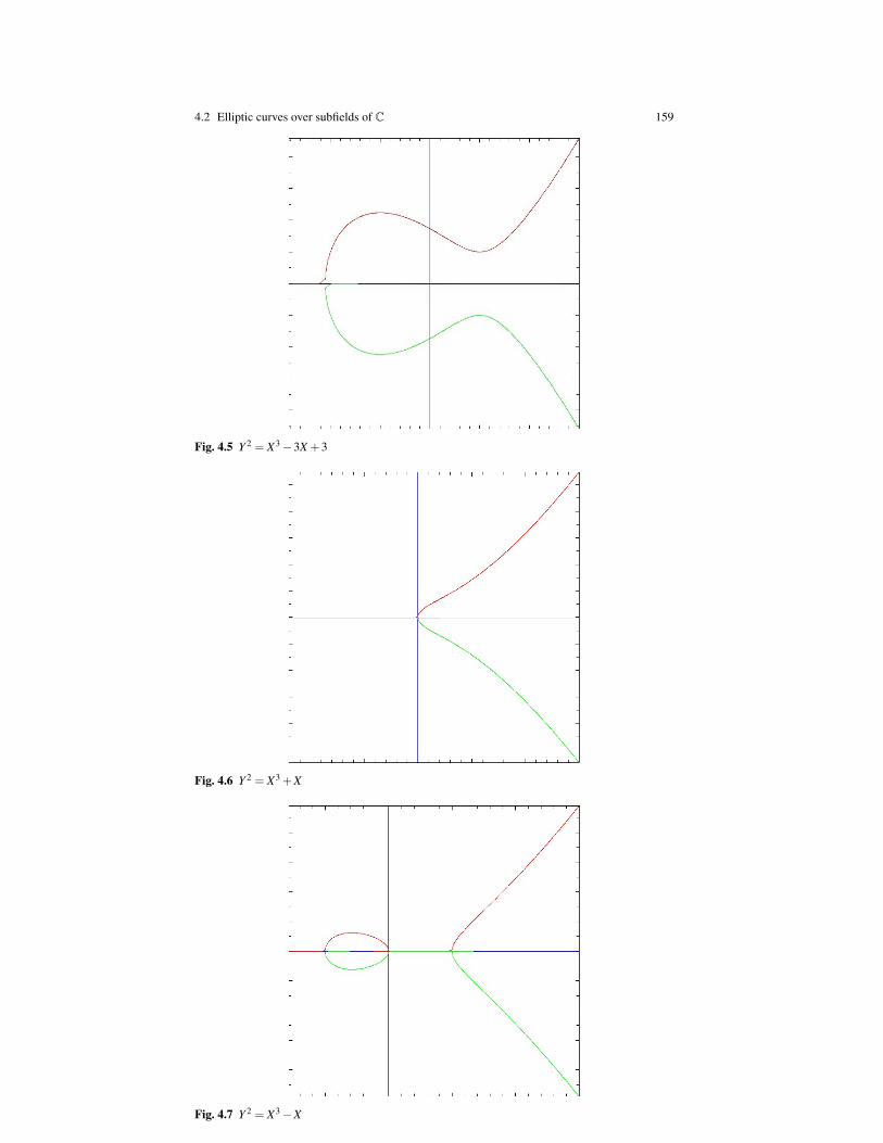
4.2 Elliptic curves over subfields of C 159
Fig. 4.5 Y 2 = X3−3X +3
Fig. 4.6 Y 2 = X3 +X
Fig. 4.7 Y 2 = X3−X
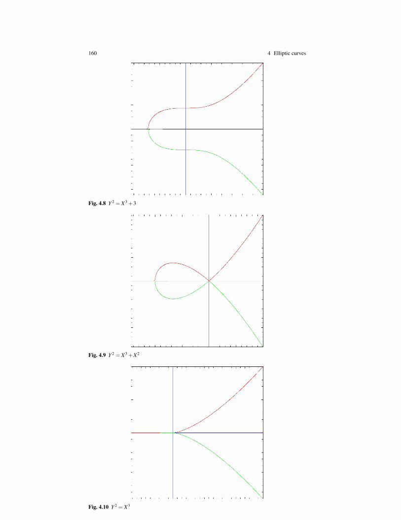
160 4 Elliptic curves
Fig. 4.8 Y 2 = X3 +3
Fig. 4.9 Y 2 = X3 +X2
Fig. 4.10 Y 2 = X3

4.2 Elliptic curves over subfields of C 161
Lemma 4.30 prepares the proof of Theorem 4.31 and the Definition 4.32 of thegroup structure of an elliptic curve (E/k,O). The lemma shows that for a pair (p,q)of distinct points from E the divisor
D := P−Q ∈ Div(E)
cannot be a principal divisor. Note that the lemma gives also a second proof ofCorollary 1.9.
Lemma 4.30 (No single pole of order one). Consider an elliptic curve (E/k,O)defined over a field k. There is no ratiomal function f ∈ k(E)∗ with
div f = P−Q
with P, Q ∈ Div(E) the elementary divisors of two distinct points p 6= q ∈ E.
Proof. Consider the point divisor
Q ∈ Div(E) of degree deg Q = 1.
Lemma 4.21 impliesdim H0(E,OQ) = 1.
Hence the inclusionk ⊂ H0(E,OQ)
impliesk = H0(E,OQ).
Hence each f ∈ H0(E,OQ) is constant, and therefore f = 0 or
div f = 0 ∈ Div(E)
which implies p = q, a contradiction, q.e.d.
Lemma 4.30 shows: The obstructions for a divisor D ∈Div0(E) to be a principaldivisor are divisors of type P−Q or even of type P−O∞. A divisor D ∈ Div0(E) isthe divisor of a rational function up to a divisor of type
P−O∞.
Because the point P ∈ E is uniquely determined by D, the obstruction is expressedby P alone.
We use the notation from Definition 4.19).
Theorem 4.31 (The class group of degree zero divisors on an elliptic curve).Consider an elliptic curve (E/k,O).

162 4 Elliptic curves
1. For any divisor D ∈ Div0(E) exists a unique point p ∈ E with
D∼ P−O∞
Denote the corresponding map by
σ : Div0(E)→ E, D 7→ p.
2. The map σ is surjective. It induces a bijective map from the group of divisorclasses of degree = 0
σ : Cl0(E)'−→ E
with inverseE '−→Cl0(E), p 7→ [P−O∞].
Proof. 1. Definition of σ : The divisor D+O∞ has degree = 1. Lemma 4.21 implies
dim H0(E,OD+O∞) = 1.
We choose a non-zero rational function f ∈ k(E)∗ with divisor satisfying
div f ≥−(D+O∞).
Becausedeg (div f ) = 0 but deg(−(D+O∞)) =−1,
there exists a point p ∈ E with
div f =−(D+O∞)+P
Then0∼−(D+O∞)+P i.e. D∼ P−O∞.
If for a different pointq ∈ E, q 6= p,
alsoD∼ Q−O∞
then0 = D−D∼ P−Q.
Hence for a suitable rational function g ∈ k∗(E)
P−Q = div g,
contradicting Lemma 4.30. Therefore
σ(D) := p ∈ E
is well-defined.
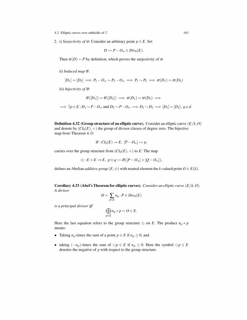
4.2 Elliptic curves over subfields of C 163
2. i) Surjectivity of σ : Consider an arbitrary point p ∈ E. Set
D := P−O∞ ∈ Div0(E).
Then σ(D) = P by definition, which proves the surjectivity of σ .
ii) Induced map σ :
[D1] = [D2] =⇒ P1−O∞ ∼ P2−O∞ =⇒ P1 ∼ P2 =⇒ σ(D1) = σ(D2)
iii) Injectivity of σ :
σ([D1]) = σ([D2]) =⇒ σ(D1) = σ(D2) =⇒
=⇒ ∃p∈E : D1∼P−O∞ and D2∼P−O∞ =⇒ D1∼D2 =⇒ [D1] = [D2], q.e.d.
Definition 4.32 (Group structure of an elliptic curve). Consider an elliptic curve (E/k,O)and denote by (Cl0(E),+) the group of divisor classes of degree zero. The bijectivemap from Theorem 4.31
σ : Cl0(E)−→ E, [P−O∞] 7→ p,
carries over the group structure from (Cl0(E),+) to E: The map
⊕ : E×E −→ E, p⊕q := σ([P−O∞]+ [Q−O∞]),
defines an Abelian additive group (E,⊕) with neutral element the k-valued point O ∈ E(k).
Corollary 4.33 (Abel’s Theorem for elliptic curves). Consider an elliptic curve (E/k,O).A divisor
D = ∑p∈E
np ·P ∈ Div0(E)
is a principal divisor iff ⊕p∈E
np ∗ p = O ∈ E.
Here the last equation refers to the group structure ⊕ on E. The product np ∗ pmeans:
• Taking np-times the sum of a point p ∈ E if np ≥ 0, and
• taking (−np)-times the sum of p ∈ E if np ≤ 0. Here the symbol p ∈ Edenotes the negative of p with respect to the group structure.

164 4 Elliptic curves
Proof. Because0 = deg D = ∑
p∈Enp
we haveD = D− ∑
p∈EnP ·O∞ = ∑
p∈Enp · (P−O∞) ∈ Div0(E)
Due to Theorem 4.31, part ii)
D principal ⇐⇒ [D] = 0 ⇐⇒ σ([D]) = O ∈ E ⇐⇒
⇐⇒ σ
(∑p∈E
np · [P−O∞]
)= O ∈ E ⇐⇒
⊕p∈E
np ∗σ([P−O∞]) = O ∈ E ⇐⇒
⇐⇒⊕p∈E
np ∗ p = 0 ∈ E, q.e.d.
Proposition 4.34 (Group structure of tori and elliptic curves). For a complextorus T = C/Λ the biholomorphic map from Theorem 4.3
φ : T −→ E(C)
onto the complex points of a plane elliptic curve E is an isomorphism of groups.
Proof. 1. i) Denote by 0T ∈ T the neutral element of the group (T,⊕). The canoni-cal morphism
ρ : (T,⊕)−→ (Div0(T ),+), p 7→ 1 · p−1 ·0T ,
is a group morphism: For j = 1,2 and two points p j ∈ T and divisors fromDiv0(T )
D j := 1 · p j−1 ·0T and D := 1 · (p1⊕ p2)−1 ·0T
the difference
D1 +D2−D = 1 · p1 +1 · p2−1 · (p1⊕ p2)−1 ·0T ∈ Div0(T )
is a principal divisor according to Abel’s Theorem 1.21 because
p1⊕ p2 (p1⊕ p2)0T = 0T ∈Λ
ii) For a point p ∈ T the image
ρ(p) = 1 · p−1 ·0T ∈ Div0(T )
is a principal divisor iff p = 0T , again due to Abel’s Theorem. If we denote by
ρ : T −→Cl0(T )

4.2 Elliptic curves over subfields of C 165
the composition of ρ with the canonical map Div0(T )−→Cl0(T ) then
ρ : T −→Cl0(T )
is injective.
iii) Each divisor
D = ∑a∈A
na ·a−∑b∈B
nb ·b ∈ Div0(T ), A, B⊂ T,A∩B = /0,na,nb > 0,
defines a point
p :=
(⊕a∈A
na ·a
)
(⊕b∈B
nb ·b
)∈ T
Thenρ(p) = 1 · p−1 ·0T ∈ Div0(T )
Due to Abel’s Theorem the difference
ρ(p)−D= 1
((⊕a∈A
na ·a
)
(⊕b∈B
nb ·b
))−1 ·0T−
(∑a∈A
na ·a−∑b∈B
nb ·b
)∈Div0(T )
is a principal divisor because 0T = 0T ∈Λ . Hence ρ is surjective.
iv) Part ii) and iii) imply that ρ is an isomorphism of groups.
2. Due to part 1) and Definition 4.32 the group structures respectively on domainand codomain of
φ : T −→ E(C)
are determined by the divisor class groups. Because φ is an analytical isomor-phism it is a group isomorphism, q.e.d.
Remark 4.35 (Group structure of an elliptic curve).
1. Geometric version: The group structure from Definition 4.32 of an ellipticcurve (E/k,O) can also be obtained by a geometric construction. It relies onthe fact that a cubic and a line in P2 intersect in exactly three points, countedwith multiplicity.
See Figure 4.11: Two add two points p,q ∈ E \ O consider the line L(p,q)passing through p and q. The line intersects E in a third point r ∈ E. The secondline L(r,O) intersects E in a third point, which is p⊕q. For more details see [63].

166 4 Elliptic curves
Fig. 4.11 Group law on an elliptic curve (Geometric construction)
2. Mordells theorem: The group structure on E(Q) provides also the set E(K)of K-valued points with a group structure for any intermediate field
Q⊂ K ⊂Q.
Mordell proved: The Abelian group E(Q) of Q-valued points of E is finitelygenerated, [56, Chap. VIII, Theor. 4.1]. As a consequence, E(Q), today namesthe Mordell-Weil group of E/Q, decomposes as the product of an Abelian torsiongroup and a free Abelian group of finite rank r < ∞
E(Q) = E(Q)tors×Zr.
Many open questions are related to the rank r.
3. Falting’s theorem: Elliptic curves have genus g = 1. Curves of genus g > 1do no longer carry a group structure. Mordell conjectured: Projective algebraiccurves C/Q with genus g > 1 have only finitely many points with rational coor-dinates, i.e.

4.2 Elliptic curves over subfields of C 167
card C(Q)< ∞.
The Mordell-conjecture was proved by Faltings, see [58].
Example 4.36 (Group structure of an elliptic curve). Consider an elliptic curve E/Q.The PARI file Elliptic_curve_torsion_group investigates the torsiongroup of E(Q) for the elliptic curve E/Q with Weierstrass polynomial
y2 = x3−43x+166
see Figure 4.12. It shows that the torsion group E(Q)tors has a factor isomorphicto Z/7Z. For more information, in particular for the equality
E(Q)tors = Z/7Z
see [54, Chap. VII, Theor. 7.5]. It is conjectured that the rank r of the free part ofthe group E(Q) equals the analytic rank of E/Q.

168 4 Elliptic curves
Fig. 4.12 The group E(Q)tors

4.3 Elliptic curves over finite fields 169
4.3 Elliptic curves over finite fields
The present section starts the investigation of elliptic curves defined over Q. Eachelliptiv curve E/Q can also be defined by a distinguished Weierstrass polynomialwith integer coefficients, called a global minimal polynomial, see Definition 4.37and Remark 4.38.
Entering into the field of arithmetic geometry one may reduce the integer equa-tion modulo any prime p ∈ Z, each time obtaining an elliptic curve defined over afinite field Fp. Considered from a general point of view: An elliptic curve definedover Q is a family of not necessarily smooth curves defined over all prime fields ofprime characteristic. Or even more general, it is a map to Spec Z, and all but butfinitely many fibres are elliptic curves over prime fields. Reduction modulo p is apowerful tool to investigate the arithmetic information encoded in an elliptic curvedefined over Q.
Before investigating the family of elliptic curves one has to eliminate redundantprime powers of the discriminant which otherwise would distort the result. The dis-criminants of the different Weierstrass polynomials of an elliptic curve differ bya non-zero rational. After multiplying with a principal nominator they differ by anon-zero integer. Hence the reduction of the discriminants modulo a prime p ∈ Zmay differ. To generalize the discriminant criterion from Proposition 4.26 one hasto find a unique minimal discriminant. The corresponding Weierstrass polynomialis named global minimal.
Definition 4.37 (Global minimal Weierstrass polynomial). For an elliptic curve E/Qa Weierstrass polynomial F ∈ Z[X ,Y ] with integer coefficients is global minimal ifits discriminant
∆F =± ∏p prime
pv(p), v(p) ∈ N∗,
is minimal for each given prime factor p of ∆F in the following sense: The ellipticcurve E/Q cannot be defined by a Weierstrass polynomial Fp(X ,Y ) ∈ Z[X ,Y ] withdiscriminant ∆Fp satisfying
ordp(∆Fp)< v(p).
“Global minimality” is a global property because it refers to all primes of ∆F
Remark 4.38 (Global minimal Weierstrass polynomial).
1. Non-uniqeness of the discriminant: The Weierstrass polynomial of an ellipticcurve, even if is in short form, is not uniquely determined. In general, an el-liptic curve does not have a unique discriminant. It is not the discriminant, butthe j-invariant which characterizes the elliptic curve.

170 4 Elliptic curves
2. Global minimal Weierstrass polynomial: The discriminant of a global minimalWeierstrass polynomial
F(X ,Y ) ∈ Z[X ,Y ]
is uniquely determined. The last condition from Definition 4.37 implies for anyprime factor p 6= 2,3 of its discriminant
ordp(∆F)< 12.
Each elliptic curve over k =Q has a global minimal Weierstrass polynomial. Theresult generalizes to elliptic curves over arbitrary number fields with class num-ber = 1, see [56, Chap. VIII, Cor. 8.3] and more specific [33, Theor. 10.3]. Aglobal minimal Weierstrass polynomial is not necessarily in short form.
3. PARI command: The Pari command ellminimalmodel provides the global mini-mal model for elliptic curves over number fields k with class number = 1.
Example 4.39 (Global minimal Weierstrass polynomial).
1. See PARI-file Elliptic_curve_weierstrass_equation_12. Figure 4.13,upper example, considers the Weierstrass polynomial
F(X ,Y ) = Y 2− (X3 +15.625)
Its discrimant∆F =−24 ·33 ·512
is not minimal because512|∆F
The global minimal Weierstrass polynomial is
Fmin(X ,Y ) = Y 2− (X3 +1)
with discriminant∆Fmin =−24 ·33.

4.3 Elliptic curves over finite fields 171
Fig. 4.13 Global minimal Weierstrass polynomial
2. The Weierstrass polynomial
F(X ,Y ) = Y 2− (X3−595 ·X +5.586) ∈ Z[X ,Y ]
with discriminant∆F = 212 ·73
is global minimal, despite of the exponent 12 of the particular prime factor p = 2.
3. Consider the elliptic curve E/Q with Weierstrass polynomial in short form
F(X ,Y ) = Y 2− (X3 +15·X +1) ∈Q[X ,Y ]
which is not global minimal because it has a non-integer cefficient. To obtain aglobal minimal Weierstrass polynomial, we make the transformation(
XY
)=
(u−2 ·X ′u−3 ·Y ′
)with u := 5
and multiply by u6. We obtain the Weierstrass equation
Y ′2 = X ′3 +1u·u−2 ·u6 ·X ′+u6 i.e. Y ′2 = X ′3 +53 ·X ′+56
Hence E/Q is also defined by the Weierstrass polynomial
Fmin(X ,Y ) = Y 2− (X3 +53 ·X +56) ∈ Z[X ,Y ]
which is global minimal because
∆Fmin =−24 ·59 ·31 ·109 ∈ Z,

172 4 Elliptic curves
see Figure 4.13, lower example.
Definition 4.40 (Reduction mod p). Consider an elliptic curve
E = (E/Q,O)
with global minimal Weierstrass polynomial F(X ,Y ) ∈ Z[X ,Y ].
1. Denote byFhom ∈ Z[X0,X1,X2]
the homogeniziation of F . For each prime p ∈N reducing mod p the coefficientsof Fhom provides a Weierstrass polynomial
Fhom,p ∈ Fp[X0,X1,X2]
with coefficients from the finite field Fp. The Weierstrass polynomial defines theprojective variety
Ep :=Var(Fhom,p) := (x0 : x1 : x2) ∈ P2(Fp) : Fhom,p(x0,x1,x2) = 0 ⊂ P2(Fp),
which is named the reduction mod p of E .
2. At a prime p ∈ Z the elliptic curve E is
• stable if (Ep,O) is non-singular, i.e. an elliptic curve over Fp.
• semistable if (Ep,O) is singular with a node.
• unstable if (Ep,O) is singular with a cusp.
3. The conductor cond(E)∈N∗ of E/Q distinguishes the primes p with semistablereduction from those with unstable reduction: One has
cond(E) = ∏p
pep
with the same prime factors p as the discriminant ∆F . The exponents of the primefactors satisfy
ep := 1 ⇐⇒ E is semistable at p
and for p > 3ep := 2 ⇐⇒ E is unstable at p,
For p = 2, 3 see also [54, App. C, §16].

4.3 Elliptic curves over finite fields 173
According to Proposition 4.26 the distinction between stable and not-stable at aprime p depends on the reduction of the minimal discriminant. The followingexample 4.41 shows why it is necessary to study elliptic curves by consideringglobal minimal Weierstrass polynomials, not just arbitrary Weierstrasspolynomials.
Example 4.41 (Reduction mod p of a global minimal Weierstrass polynomial). Con-sider the elliptic curve (E/Q,O) from Example 4.39 defined by the inhomogeneousWeierstrass polynomial
F(X ,Y ) = Y 2− (X3 +15.625) ∈Q[X ,Y ]
with discriminant∆F =−24 ·33 ·512 ∈ Z.
Note 15.625 = 56.
i) The Weierstrass polynomial F ∈ Z[X ,Y ] is in short form but it is not globalminimal. Reducing its coefficients mod p = 5 gives the Weierstrass polynomial inshort form
F5(X ,Y ) = Y 2−X3 ∈ F5[X ,Y ]
with discriminant∆F5 = 0 ∈ F5.
Hence the Weierstrass polynomial F5 defines a singular cubic over F5 with a cusp.Note that the discriminant ∆F contains the prime factor 512.
ii) Therefore we have to apply first the coordinate transformation with the matrix(1/u2 0
0 1/u3
), u := 5,
which transforms F(X ,Y ) to the global minimal Weierstrass polynomial
F ′(X ′,Y ′) = Y ′2− (X ′3 +1)
with discriminant∆F ′ =−24 ·33 ∈ Z.
Reducing the coefficients of F ′ mod p = 5 creates the Weierstrass polynomial
F ′5(X′,Y ′) = Y ′2− (X ′3 +1) ∈ F5[X ′,Y ′]
with discriminant∆F ′5
= 3 ∈ F5.
The reduction of E mod p = 5 defines an elliptic curve E5 over F5.

174 4 Elliptic curves
Remark 4.42 (Hasse estimate).
1. Important properties of an elliptic curve E/Q are encoded in the function, whichattaches to each prime p with stable Ep the family
Ep(Fpn), n ∈ N∗,
of orders of the groups of Fpn -valued points of the elliptic curve Ep. These groupscollect those points from Ep ⊂ P2(F p) with all coordinates in the finite fields Fpn .
We recall the following result of Hasse for the case n = 1:∣∣1+ p− card Ep(Fp)∣∣≤ 2 ·√p.
For a proof see [33, Theor. 10.5].
Hasse’s result was conjectured by Artin. The value
1+ p
for comparison is motivated as follows: The field Fp has p elements. AWeierstrass equation
Y 2 = X3 +AX +B
is quadratic in Y . Hence for each x ∈ Fp there exist at most twosolutions (x,y) ∈ A2(Fp). Taking into account the point at infinity O ∈ Ep(Fp)gives the estimate
card Ep(Fp)≤ (1+2p).
In the average, i.e. by choosing the Weierstrass polynomial at random, onecould expect a 50% chance to find a solution (x,y) at all. Therefore 1+ p is aplausible average for card Ep(Fp).
One defines for any prime p the difference
ap(E) := 1+ p− card Ep(Fp)
between the average number and the actual number of Fp-valued points of E.
2. See the PARI-file Elliptic_curve_Hasse_estimate_05 for the numer-ical example of the Hasse inequality displayed in Figure 4.14.

4.3 Elliptic curves over finite fields 175
Fig. 4.14 The Hasse estimate
3. The sequence(ap(E))p prime
will turn out to be a fundamental characteristic of the elliptic curve E, seeRemark 4.45. These numbers determine also the cardinalities
card Ep(Fpn)
for n≥ 2. The latter will serve as the generators of the ζ -function of E, seeDefinition 4.44.

176 4 Elliptic curves
Historically, the first example of a ζ -function is due to by L. Euler. The functionhas later be named Riemann ζ -function
Proposition 4.43 (ζ -function and Euler product). The Riemann ζ -function
ζ : s ∈ C : Re s > 1 −→ C, ζ (s) :=∞
∑n=1
1ns
is holomorphic. The ζ -function
1. extends to a meromorphic function on C with a single pole at s = 1. The pole hasorder = 1 and residue = 1.
2. It satisfies the functional equation with respect to reflection at the point s = 1
π−s/2 ·Γ (s/2) ·ζ (s) = π
−(1−s)/2 ·Γ ((1− s)/2) ·ζ (1− s)
with the Γ -function,
3. and it has the product representation
ζ (s) = ∏p
11− p−s
with the product taken over all primes p.
Proof. 1. See [64, Teil I, § 4].
2. See reference from part 1).
3. For each N ∈ N expand the finite product by using the geometric series and theunique prime factor decomposition of integers
∏p<N
11− p−s = ∏
p<N
(1+
1ps +
1p2s + ...
)= ∑
′ 1ns
with the sum on the right-hand side taken over all positive integers with all primefactors less than N. The limit N→ ∞ proves the claim, q.e.d.
From the viewpoint of the ring Z the Riemann ζ -function is a global object.Because it considers all primes p∈Z and collects as a product the local informationencoded in the geometric series of p
11− p−s =
∞
∑n=0
(1/p−s)n
Apparently, all information about a prime p is just its value.

4.3 Elliptic curves over finite fields 177
We now switch from the primes p of Z to the elliptic curves Ep/Fp, which are thefibres of a given elliptic curve E/Q over its stable primes p. First we study thelocal information, i.e. the information encoded in Ep/Fp. The curve Ep contributesas local information at the prime p the sequence of cardinalities of points withvalues in the finite fields of characteristic p
card Ep(Fpn), n ∈ N∗.
Definition 4.44 (Zeta-function of an elliptic curve over Fp). Consider an ellipticcurve Ep/Fp. The ζ -function of Ep is the formal power series with generator derivedfrom the sequence (card Ep(Fpn))n∈N∗
Z(Ep,T ) := exp
(∞
∑n=1
card Ep(Fpn) ·T n
n
)∈Q[[T ]].
One checks by formal derivation
T ·d
dTlog Z(Ep,T )=T ·
Z′
Z=T ·
∞
∑n=1
(card Ep(Fn
p) ·T n−1)= ∞
∑n=1
(card Ep(Fn
p) ·T n)
Remark 4.45 (Properties of the ζ -function of an elliptic curve over Fp). The ζ -functionof an elliptic curve Ep/Fp
Z(Ep,T ) ∈Q[[T ]]
has the following properties:
1. Rationality: The ζ -function is a rational function over the ring Z, more precisely:
Z(Ep,T ) =L(Ep,T )
(1−T ) · (1− p ·T )∈ Z(T )
with the quadratic polynomial
L(Ep,T ) = 1−ap(E) ·T + p ·T 2, ap(E) := 1+ p− card Ep(Fp).
2. Functional equation: The ζ -function satisfies the functional equation
Z(Ep,1/pT ) = Z(Ep,T ).
3. Analogue of the Riemann hypothesis: Both complex zeros α, β ∈ C of L(Ep,T )have modulus
|α|= |β |=√p.

178 4 Elliptic curves
The proof of these properties is due to Weil, [56, Chap. V, Theor. 2.2].
Weil also stated and proved a generalization for projective algebraic curvescurves Cp/Fp of arbitrary genus. If the curve Cp is the reduction mod p of a curve
C/Q
then Weil’s theorem shows the neat relation between the curve Cp and the complexcurve X(C)⊂ Pn: The dimension of the polynomial in the numerator ofthe ζ -function of Cp is the first Betti number of the compact Riemann surface X/C.
Moreover, Weil made a conjecture for the general case of higher-dimensionalsmooth projective algebraic varieties. Deligne proved the Weil conjecture. For anexcellent introduction to the whole subject see [29, Appendix C].
The L-series L(E) of an elliptic curve E/Q collects for each prime p ∈ Z thelocal information about the reduction Ep. Hence the L-series is a global object.
Definition 4.46 (L-series of an elliptic curve over Q). The L-series of an ellipticcurve E/Q is the function
L(E,−) : s ∈ C : Re s > 3/2→ C, L(E,s) := ∏p
1Z(Ep, p−s)
Remark 4.47 (L-series of an elliptic curve E/Q).
1. The convergence of the L-series and its representation as an absolut convergentDirichlet series with respect to the variable s follows from Hasse’s estimate inRemark 4.42 and the theory of Euler products, see [33, Chap. X, Cor. 10.6].Hence L(E) is a holomorphic function.Due to the proof of the Shimura-Taniyama-Weil conjecture the L-series ofan elliptic curve extends holomorphically to the whole complex plane. Thereare several unsolved conjectures about the arithmetic information encoded bythe L-series of an elliptic curve. E.g. Birch and Swinnerton-Dyer conjectured
rank E(Q) = r
with r equal to the analytic rank defined as the order of the zero of the L-seriesat s = 1
r := ord(L(E); 1).
The PARI script Elliptic_curve_04_2 computes the analytic rank forsome elliptic curves E/Q of higher analytic rank, see Figure 4.15.
For more results and conjectures see [56, App. C, § 16].

4.3 Elliptic curves over finite fields 179
2. The two polynomials in the denominator of the ζ -function Z(Ep,T ) evaluateat T = p−s as values of the Riemann ζ -function
11− p−s = ζ (s) and
11− p1−s = ζ (s−1)
They do not provide new information about the elliptic curve.
3. If one compares the L-series L(E,s) of an elliptic curve E/Q with the Riemann ζ -function ζ (s)on the level of the two product representations
L(E,s) = ∏p
1Z(Ep, p−s)
and ζ (s) = ∏p
11− p−s
then for each given prime p the local factor
Z(Ep, p−s) corresponds to1
1− p−s
The geometric series on the right hand side depends only on the prime p, whilethe corresponding ζ -function on the left-hand side depends on p and on the re-duction of the given elliptic curve E/Q.

180 4 Elliptic curves
Fig. 4.15 Analytic rank of several elliptic curves E/Q

Chapter 5Introduction to Hecke theory and applications
5.1 Hecke operators of the modular group and their eigenforms
Definition 5.1 (Multiplicative function). A function
f : N∗ −→ N∗
is muliplicative if for each pair of coprime integers m, n ∈ N∗ holds
f (n ·m) = f (n) · f (m)
Proposition 5.2 (Multiplicativeness of the power sum function). For each k ∈Nthe function
σk : N∗ −→ N∗, σk(n) := ∑d|n
dk,
is multiplicative. It has the product representation
σk(n) =N
∏j=1
p(e j+1)kj −1
pkj−1
Proof. The prime decomposition
n =N
∏j=1
pe jj , n ∈ N∗,
and the formula for the finite geometric series imply the product formula
σk(n) =(
pk1 + pk·2
1 + ...+ pk·e11
)· ... ·
(pk
N + pk·2N + ...+ pk·eN
N
)=
181

182 5 Introduction to Hecke theory and applications
=N
∏j=1
(e j
∑ν=1
(pk
j
)ν
)=
N
∏j=1
p(e j+1)kj −1
pkj−1
And the product formula implies for coprime n,m ∈ N∗
σk(n) ·σk(m) = σk(n ·m), q.e.d.
Corollary 5.3 (Eisenstein series are multiplicative). For each even k ≥ 4 theFourier coefficents of the Eisenstein series
−Bk
2k·Ek(τ) =
∞
∑ν=0
cν ·qν , q = e2πi·τ ,
are multiplicative for ν ≥ 1.
Proof. We reduce the statement of the corollary to Proposition 5.2: Corollary 3.11shows
Ek(τ) = 1−2kBk·
∞
∑ν=1
σk−1(ν) ·qν , q = e2πi·τ
and−Bk
2k·Ek(τ) =
−Bk
2k+
∞
∑ν=1
σk−1(ν) ·qν ,
with Fourier coefficents
cν = σk−1(ν), ν ≥ 1, q.e.d.
Corollary 5.3 starts with the multiplicativeness of a well-known arithmetic func-tion and derives the multiplicativeness of the Fourier coefficients of certain modularforms. Hecke theory goes the way in the opposite direction: Hecke operators singleout certain modular forms and derive the multiplicativeness of their Fourier coeffi-cients. Historically the first example is the normalized discriminant form
∆
(2π)12
which gives the multiplicativeness of Ramanujan’s τ-function.
Hecke operators are linear maps on modular forms, more precisely: For eacheven weight k ∈ N the Hecke algebra
Hk(Γ )⊂ End(Mk(Γ ))
is a commutative subalgebra of endomorphisms, which restrict to endomorphismsof the vector spaces of cusp forms Sk(Γ ) ⊂ Mk(Γ ). For fixed weight the Heckealgebra Hk(Γ ) is generated by a family of Hecke operators (Tm)m∈N. They average
5.1 Hecke operators of the modular group and their eigenforms 183
the transformation behaviour of modular forms with respect to certain equivalenceclasses of matrices
Γm ⊂ GL(2,R)+
The equivalence classes are the orbits of a left action of the modular group on thesematrices, which we have to study first.
Besides the two sequences of levels N ∈N∗ from Definition 2.9 and weights k ∈ Zfrom Definition 3.6 we now introduce a third sequence m ∈ N∗. It is the sequenceof the sets of integral matrices with determinant = m, see Definition 5.4. These ma-trices generalize the modular group Γ with respect to the determinant. They serveto define the Hecke operators which average the values of modular forms of a givenweight and level. In addition, these integral matrices will serve in Section 6.2 toaverage as class invariants distinguished values of the j-invariant.
Definition 5.4 (Integral matrices with positive determinant). For any m ∈ N∗consider the set of matrices
Γm := M ∈M(2×2,Z) : det M = m ⊂ GL(2,Q)+
and its subset
Γm,prim :=(
a bc d
)∈ Γm : (a,b,c,d) = 1
of primitive matrices. We denote by
Φm : Γ ×Γm→ Γm,(A,M) 7→ A ·M
the canonical Γ -left action, and by
Φm,prim := Φm|Γm,prim : Γ ×Γm,prim −→ Γm,prim
its restriction. The respective orbits sets are denoted as the left quotients
Γ \Γm and Γ \Γm,prim.
Remark 5.5 (Restriction of the Γ -action to the primitive matrices). The subset
Γm,prim ⊂ Γm
is stable under the Γ -left action Φm.
Proof. For the proof consider any
A =
(α β
γ δ
)∈ Γ and M =
(a bc d
)∈ Γm,prim.

184 5 Introduction to Hecke theory and applications
The ideal generated by the coefficients of the product matrix A ·M
I := (αa+βc,αb+βd,γa+δc,γb+δd)⊂ Z
contains the element
δ · (αa+βc)+(−β ) · (γa+δc) = (αδ −βγ)a+(δβ −βδ )c = a
and similar for b, c, d with the other generators of I. Therefore
(1) = (a,b,c,d)⊂ I
which implies(1) = I
Hence the coefficients of the product matrix A ·M are coprime, i.e.
Φm(A,M) = A ·M ∈ Γm,prim, q.e.d.
Lemma 5.6 shows that each orbit of the group action can be represented by atriangular matrix which facilitates many calculations.
Lemma 5.6 (Orbit sets of the left action). Consider a positive integer m ∈ N∗.
1. A bijective map exists
Γ \Γm'−→V (m) :=
(a b0 d
)∈ Γm : 0≤ b < d
to a subset of upper triangular matrices. The orbit set of Φm has cardinality σ1(m).
2. A bijective map exists
Γ \Γm,prim'−→V (m, prim) :=
(a b0 d
)∈V (m) : (a,b,d) = 1
.
The orbit set of Φm,prim has cardinality
ψ(m) := m · ∏p|m
p prime
(1+(1/p))
Proof. 1. We define a mapp : Γm→V (m),
which attaches to each M ∈Γm a distinguished triangular matrix p(M) belongingto the same orbit. And we show that the matrix p(M) depends only on the orbitof M:

5.1 Hecke operators of the modular group and their eigenforms 185
i) Consider a fixed but arbitrary element
M =
(a bc d
)∈ Γm.
We construct a matrix
A =
(α β
γ δ
)∈ Γ
such that
A ·M =
(αa+βc αb+βdγa+δc γb+δd
)∈V (m) :
First, in order to remove the entry c of M we choose coprime integers γ,δ ∈ Zwith
γ ·a+δ · c = 0.
In order to obtain a matrix with det = 1 we choose integers α,β ∈ Z with
α ·δ −β · γ = 1.
Such a choice is possible because γ and δ are coprime. Set
A1 :=(
α β
γ δ
)∈ Γ .
Then
A1 ·M =
(a′ b′
0 d′
)and
det (A1 ·M) = det M = a′ ·d′ = m.
In particular d′ 6= 0 and possibly after replacing A1 by −A1 even a′, d′ > 0.
Secondly, because T ∈ Γ , for any k ∈ Z also
A2(k) := T k ·A1 ∈ Γ .
Then
A2(k) ·M =
(1 k0 1
)·(
a′ b′
0 d′
)=
(a′ b′+ k ·d′0 d′
).
We choose k0 ∈ Z such that
0≤ b′+ k0 ·d′ < d′
and setA := A2(k0).
ii) The construction from part i) determines uniquely the element
A ·M ∈V (m) :

186 5 Introduction to Hecke theory and applications
Assume two matrices Ai ∈ Γ such that
Ai ·M =: Mi ∈V (m), i = 1,2.
Then
M = A−11 ·M1 = A−1
2 ·M2 or A21 ·M1 = M2, A21 := A2 ·A−11 .
Set
A21 =:(
α β
γ δ
)and Mi :=
(ai bi0 di
), i = 1,2.
From (α β
γ δ
)·(
a1 b10 d1
)=
(a2 b20 d2
)follows:
• γ ·a1 = 0, hence γ = 0.
• From d2 = δ ·d1 follows δ > 0. Together with α ·δ = 1 it implies α = δ = 1.
• As a consequence a1 = a2, d1 = d2, and b1 +β ·d1 = b2.
• Because 0≤ b1,b2 < d1 = d2 we get b1 = b2 and β = 0.
As a consequence
A21 =
(1 00 1
)or A1 = A2.
iii) Part i) and ii) show that
p : Γm→V (m), M 7→ A ·M,
is well-defined, and p(M) belongs to the same orbit as M.
iv) The map p is surjectice because V (m)⊂ Γm. In addition,
p(M1) = p(M2) ⇐⇒ ∃ A ∈ Γ with A ·M1 = M2
⇐⇒ M1 and M2 on the same orbit of Φm.
As a consequence p induces the bijective map
Γ \Γm'−→V (m), M 7→ p(M).
v) The equalitycard V (m) = σm(1)
follows at once from the explicit representation of the elements of V (m): Eachcoefficient d ≥ 0 satisfies d|m and allows d different coefficients b.

5.1 Hecke operators of the modular group and their eigenforms 187
2. The representation of the orbit set Γ \Γm,prim follows from part 1) by restriction.For the cardinality of V (m, prim) see [38, Chap. 5, §1].
Corollary 5.7 (Complete representatives of the orbit set). For each γ ∈ Γ :
1. The setV (m) · γ ⊂ Γm
is a complete set of representatives of the orbit set Γ \Γm, i.e. with respect to thecanonical projection
Γm→ Γ \Γm, M 7→ [M],
holds the equality of sets
Γ \Γm = [M] : M ∈V (m)= [M · γ] : M ∈V (m).
2. The setV (m, prim) · γ ⊂ Γm,prim
is a complete set of representatives of the orbit set Γ \Γm,prim.
Proof. 1. Consider a given γ ∈Γ . We show: For arbitrary but fixed M ∈V (m) existan element
M1 ∈V (m)
and a unique matrix A ∈ Γ such that
A ·M = M1 · γ.
According to Lemma 5.6, applied to M ·γ−1 ∈Γm, a unique element A ∈Γ existswith
M1 := A · (M · γ−1) ∈V (m).
ThenM1 · γ = A ·M.
Hence M1 · γ lies on the same orbit as M. As a consequence, the map
V (m)−→V (m), [M] 7→ [M · γ],
is well-defined and injective.
2. Analogously, q.e.d.
Lemma 5.8 (Complete sets of common representatives for left/right-action).Consider an arbitrary but fixed prime p, and the left action
Φle f t : Γ ×Γp −→ Γp,(γ,M) 7→ γ ·M
188 5 Introduction to Hecke theory and applications
1. Besides the set V (p) from Lemma 5.6 the set of symmetric matrices
Vsym :=(
p 00 1
)∪(
1 bb p+b2
): 0≤ b < p
is a complete set of representatives of Φle f t too.
2. Consider a complete set V of representatives of Φle f t formed by symmetric ma-trices. Then also the system of adjoints
V ] := M] : M ∈ V , M] := (det M) ·M−1,
is a complete systems of representatives of Φle f t .
Proof. 1. For each 0≤ b < p(1 bb p+b2
)=
(1 0b 1
)·(
1 b0 p
)Hence the matrices (
1 bb p+b2
)and
(1 b0 p
)belong to the same orbit of Φle f t .
2. i) LetΦright : Γp×Γ −→ Γp, (M,γ) 7→M · γ,
be the corresponding right action of Γ . For each complete system V of represen-tatives of Φle f t the set of transposed elements
V > := v> : v ∈ V
is a complete system of representatives of Φright : Assume v∈Γp. Then also v> ∈ Γpand
v> = A ·M
for suitableA ∈ Γ and M ∈ V .
Hencev = M> ·A>
with A> ∈ Γ> = Γ .
As a consequence, if V is formed by symmetric matrices, then V is also a com-plete system of representatives for Φright .
ii) For given w ∈ Γp set

5.1 Hecke operators of the modular group and their eigenforms 189
v := (det w) ·w−1 ∈ Γp.
Then
v = w] and det v = (det w)2 ·det w−1 = det w and w = (det v) ·v−1
Due to part i) existA ∈ Γ and M ∈ V
withv = M ·A
Thendet v = det M
andv−1 = A−1 ·M−1
andw = v−1 ·det v = A−1 · ((det M) ·M−1)
withA−1 ∈ Γ
−1 = Γ , q.e.d.
We recall a simple version of the elementary divisor theorem.
Proposition 5.9 (Elementary divisor theorem).
1. For each matrixA ∈ Γm, m ∈ N∗,
exist two matrices γ1,γ2 ∈ Γ with
γ1 ·A · γ2 =
(e1 00 e2
)satisfying the divisor relation e1|e2.
2. For each pair of primitive matrices
A1,A2 ∈ Γm,prim, m ∈ N∗,
exist two matrices γ1,γ2 ∈ Γ with
A2 = γ1 ·A1 · γ2.
Proposition 5.9 is a special case of the Smith normal form, a result which holds formatrices over principal ideal domains.
Definition 5.10 (Hecke operators of the modular group). For any positive integer m≥ 1the m-th Hecke operator is the C-linear endomorphism of the algebra of modularforms

190 5 Introduction to Hecke theory and applications
Tm : M∗(Γ )→M∗(Γ )
which is defined on Mk(Γ ), k ∈ N, as
Mk(Γ )→Mk(Γ ), f 7→ Tm f := ∑Γ \Γm
f [M]k.
Here the summation extends over an arbitrary complete set of representatives M ∈ Γmof the orbit set Γ \Γm of the left action
Γ ×Γm −→ Γm.
The value f [M]k does not depend on the choice of a representative from theorbit Γ ·M because due to Lemma 3.4: For all α ∈ Γ
f [α ·M]k = ( f [α]k)[M]k = f [M]k
E.g., the summation in Definition 5.10 of the Hecke operator Tm may extend overthe elements of V (m) or over the elements of V (m) · γ,γ ∈ Γ . Note T1 = id.
Theorem 5.11 (Fourier coefficients of Hecke transforms).
1. The Hecke operators from Definition 5.10 are well-defined, i.e. for each evenweight k and for all m≥ 1
f ∈Mk(Γ ) =⇒ Tm f ∈Mk(Γ ).
2. For a modular form f ∈Mk(Γ ) with Fourier expansion
f (τ) =∞
∑n=0
an ·qn, q = e2πi·τ ,
its Hecke transform Tm f ∈Mk(Γ ) has the Fourier expansion
(Tm f )(τ) =∞
∑n=0
bn ·qn
with Fourier coefficients
bn = ∑r>0
r∈(m,n)
rk−1 ·amn/r2 , n ∈ N,
in particularb0 = a0 ·σk−1(m) and b1 = am
3. The ideal of cusp forms is stable under all Hecke operators, i.e. for each m ∈ N∗
Tm(S∗(Γ ))⊂ S∗(Γ ).

5.1 Hecke operators of the modular group and their eigenforms 191
Due to Theorem 5.11, part 1) we will use the same notation Tm for a Hecke operatorand its restriction to a single modular space of fixed weight.
Proof. 1. To prove that Tm f is a modular form of the same weight as f we have toverify the properties from Definition 3.6:
• Appararently Tm f is holomorphic on H.
• Weakly modularity: Consider a fixed but arbitrary matrix γ ∈ Γ . We replacethe summation over the orbit set V (m) by the summation over the completeset of representatives V (m) · γ , see Corollary 5.7:
(Tm f )[γ]k = ∑M∈V (m)
( f [M]k)[γ]k = ∑M∈V (m)
( f [M · γ]k) =
= ∑N∈V (m)·γ
f [N]k = ∑M∈V (m)
f [M]k = Tm f .
• Holomorphy of Tm f at the point ∞: To compute the Fourier series of Tm f weuse the summation with
M =
(a b0 d
)∈V (m)
For the computation of
( f [M]k)(τ) = f (M(τ)) ·h(M,τ)−k · (det M)k−1
we employ the following intermediate results:
i)
exp(2πin ·M(τ)) = exp
(2πin ·
aτ +bd
)= e2πin·(aτ/d) · e2πin·(b/d), n ∈ N.
ii)
∑0≤b<d
e2πib·(n/d) =
d if d|n0 otherwise
The first case follows from
e2πib·(n/d) = 1
for each of the d summands with 0≤ b < d. The second case follows fromthe formula of the finite geometric series with argument e2πi·(n/d):
d−1
∑b=0
e2πib·(n/d) =e2πi·d·(n/d)−1e2πi·(n/d)−1
= 0

192 5 Introduction to Hecke theory and applications
iii) We have
f (M(τ)) = f
(aτ +b
d
)=
∞
∑n=0
an · exp
(2πin ·
aτ +bd
)=
=∞
∑n=0
an · exp
(2πin ·
aτ
d
)· exp
(2πin ·
bd
)Hence
d−1
∑b=0
f (M(τ)) =∞
∑n=0
d ·and ·qn(m/d), q = exp(2πinτ),
because
d−1
∑b=0
f (M(τ)) =d−1
∑b=0
(∞
∑n=0
an · e2πin(aτ)/d · e2πin(b/d)
)=
=∞
∑n=0
(an · e2πin(aτ)/d ·
d−1
∑b=0
e2πin(b/d)
)=
∞
∑n=0
and · e2πinaτ ·d =
= d ·∞
∑n=0
and ·qna = d ·∞
∑n=0
and ·qn(m/d)
Due to part ii) the third last sum retains only summands with index = nd.
We now use the representation of the orbit set Γ \Γm from Lemma 5.6 andinsert the Fourier series of f . We obtain due to the formula from part iii)
(Tm f )(τ) = ∑M∈V (m)
f [M]k(τ) = mk−1 · ∑M∈V (m)
h(M,τ)−k · f (M(τ)) =
= mk−1∑d>0d|m
1dk ·
∞
∑n=0
and ·qn(m/d) ·d = ∑d>0d|m
(md
)k−1(∞
∑n=0
and ·qn(m/d)
)=
= ∑d>0
d∈(m,n)
(md
)k−1(∞
∑n=0
an ·q(n/d)·(m/d)
)
The substitution
(d,n) 7→ (t = (n/d) · (m/d), r = m/d)
provides
n =d2 · t
m=
(dm
)2
tm =tmr2 .
5.1 Hecke operators of the modular group and their eigenforms 193
Hence
(Tm f )(τ) =∞
∑t=0
∑r>0
r|(m,t)
rk−1 ·a(tm)/r2
q t
with the inner sum being finite. Apparently, the Fourier series has no coeffi-cients with negative index. Hence Tm f is holomorphic at ∞ ∈H∗.
2. For the proof see the Fourier series from the previous part.
3. A cusp form satisfies a0 = 0. The formula for the Fourier coefficients of Tm ffrom part 2) shows that Tm f is a cusp form again, q.e.d.
The following corollary specializes the general formula from Theorem 5.11. Itgives the formula for the Fourier coefficients of the Hecke transform for prime in-dices.
Corollary 5.12 (Fourier coefficients with prime index of Hecke transforms).Consider a modular form f ∈ Mk(Γ ) with Fourier coefficients (an)n∈N. Then theFourier coefficients (bn)n∈N of its Hecke transform Tm f satisfy for each primeindex p
bp =
amp if p - mamp + pk−1 ·am/p if p|m
Proof. The claim follows from the third formula for the general case in Theorem 5.11:
• If p - m then r|(p,m) implies r = 1.
• If p|m then r|(p,m) implies r = 1 or r = p; note n = p, q.e.d.
Corollary 5.13 (Simultaneous eigenvector of all Hecke operators). The discrim-inant modular form
∆ ∈ S12(Γ )
is a simultaneous eigenform of all Hecke operators, i.e. ∆ is an eigenvector of allHecke operators
Tm ∈ End(S12(Γ )), m≥ 1.
The Fourier coefficients of the normalized discriminant modular form

194 5 Introduction to Hecke theory and applications
∆
(2π)12 =∞
∑m=1
τm ·qm
are the corresponding eigenvalues, i.e. for all m ∈ N∗
Tm(∆) = τm ·∆ .
Proof. According to Corollary 3.19 and Lemma 3.23 the vector space S12(Γ ) ofcusp forms of weight k = 12 is 1-dimensional. It has the discriminant modularform ∆ from Definition 3.13 as a basis. Hence ∆ is an eigenvector of each Heckeoperator Tm, m≥ 1. To calculate the corresponding eigenvalue we recall the Fourierexpansion of the normalized discriminant modular form from Proposition 3.14:
∆(τ)
(2π)12 =∞
∑n=1
τn ·qn, τ1 = 1.
Theorem 5.11 provides the Fourier expansion
Tm
(1
(2π)12 ·∆
)(τ) = τm ·q+O(2).
Hence by comparing the linear term of the Fourier series on both sides
Tm(∆) = τm ·∆ , q.e.d.
Example 5.14 (Hecke operators). Consider the vector space of cusp forms S28(Γ ).Due to Theorem 3.19 and Lemma 3.23
dim S28(Γ ) = 2.
The two cuspforms of weight 28
f1 := ∆ ·E44 and f2 := ∆
2 ·E4
are linearly independent because
ord( f1;∞) = 1 and ord( f2;∞) = 2.
Hence ( f1, f2) is a basis of S28(Γ ). We consider the Hecke operator
T2 : S28(Γ )−→ S28(Γ ).
The endomorphism has two distinct eigenvalues, hence it can be diagonalized. Fig-ure 5.1 shows
• the Fourier series of f1 and f2
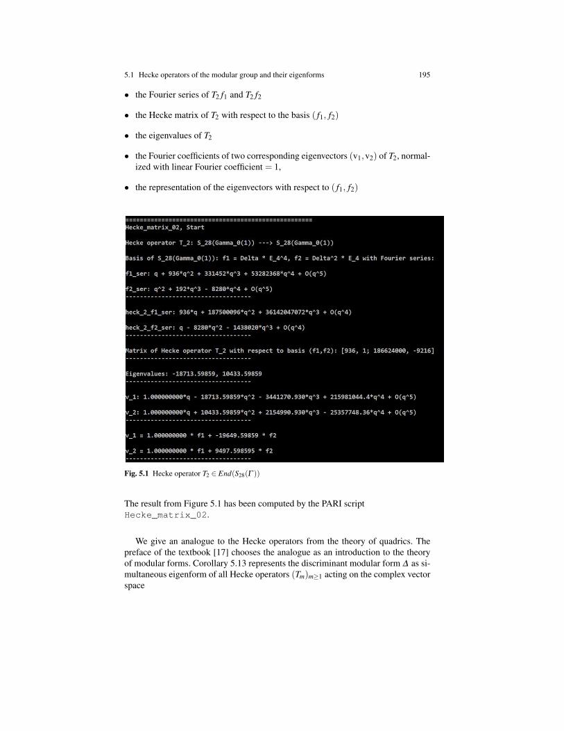
5.1 Hecke operators of the modular group and their eigenforms 195
• the Fourier series of T2 f1 and T2 f2
• the Hecke matrix of T2 with respect to the basis ( f1, f2)
• the eigenvalues of T2
• the Fourier coefficients of two corresponding eigenvectors (v1,v2) of T2, normal-ized with linear Fourier coefficient = 1,
• the representation of the eigenvectors with respect to ( f1, f2)
Fig. 5.1 Hecke operator T2 ∈ End(S28(Γ ))
The result from Figure 5.1 has been computed by the PARI scriptHecke_matrix_02.
We give an analogue to the Hecke operators from the theory of quadrics. Thepreface of the textbook [17] chooses the analogue as an introduction to the theoryof modular forms. Corollary 5.13 represents the discriminant modular form ∆ as si-multaneous eigenform of all Hecke operators (Tm)m≥1 acting on the complex vectorspace

196 5 Introduction to Hecke theory and applications
V := S12(Γ ).
The corresponding eigenvalues are the Fourier coefficients of ∆ . Remark 5.15 trans-lates the law of quadratic reciprocity from algebraic number theory into a similarshape.
Remark 5.15 (Reduction of quadrics mod p).
1. The Legendre symbol considers an odd prime p ∈ Z, and determines for eachinteger d ∈ Z whether d is a square mod p. The Legendre symbol is defined as
(dp
):=
+1 d 6≡ 0 mod p and d quadratic rest mod p−1 d 6≡ 0 mod p and d not quadratic rest mod p0 d ≡ 0 mod p
The law of quadratic reciprocity relates the Legendre symbol of two odd primesp 6= q according to the formula
(pq
)=
(
qp
)p≡ 1 mod 4 or q≡ 1 mod 4
−(
qp
)p≡ 3 mod 4 and q≡ 3 mod 4
2. Consider an arbitrary, but fixed integer d 6= 0 and the quadratic polynomial
F(X) := X2−d ∈ Z[X ]
which defines the affine quadric Q/Q
x ∈ C : F(x) = 0.
For each prime p we consider the reduction mod p
Fp(X) := X2−dp ∈ Fp[X ]
and the set Q(Fp) of points of Q with coordinates from Fp.
Analogously to Remark 4.42 for elliptic curves we define
ap(Q) := card Q(Fp)−1.
The number 1 in the definition is the average number of solutions mod p. Thevalues ap(Q) extend from prime indices to an(Q), n ∈N, and satisfy the productrule
anm(Q) = an(Q) ·am(Q), n,m ∈ N∗.
For odd prime p the number ap(Q) equals the Legendre symbol

5.1 Hecke operators of the modular group and their eigenforms 197
ap(Q) =
(dp
).
Due to the Law of Quadratic Reciprocity and its two supplements the Legendresymbol depends only on the residue class p mod 4d.
3. We now represent the sequence (ap(Q))p prime as a sequence of eigenvalues of asimultaneous eigenvector for a suitable sequence of linear endomorphisms (Tp)p prime.Our aim is to formulate an analogue of the modular group, of modular functionsand of Hecke operators:
SetN = NQ := 4|d|,
and consider the multiplicative group
G := (Z/NZ)∗,
and the complex vector space of functions defined on G
V := f : G→ C.
Eventually, as an analogue to the Hecke operators we introduce the family oflinear endomorphisms (Tp)p prime of V defined as
(Tp f )(n) :=
f (p ·n) p - N0 p | N
for n ∈ G. We claim: All endomorphism (Tp)p prime have a simultaneous eigen-vector, namely the distinguished function
fQ : G→ C, f (n) := an(Q).
Note that fQ is well-defined on the residue classes of G because the Legendresymbol depends only on the residue class p mod 4d. Computing the eigenvalueswe get for all n ∈ G
Tp( fQ)(n) =
fQ(p ·n) = apn(Q) = ap(Q) ·an(Q) p - N
0 p | N
As a consequence, for all primes p ∈ Z
Tp( fQ) = ap(Q) · fQ.
It is not by chance that in Example 5.14 the Hecke endomorphism T2 ∈End(S28(Γ ))can be diagonalized. Theorem 5.18 will show: The Hecke algebra of a given weight

198 5 Introduction to Hecke theory and applications
is commutative. And Theorem 5.26 will show that the Hecke operators are selfad-joint with respect to a certain Hermitian scalar product on the cusp forms. Hence allHecke operators on cusp forms can be simultaneously diagonalized.
Definition 5.16 (Hecke algebra of weight k). The Hecke algebra of even weight k ∈ N
Heckek(Γ )⊂ End(Mk(Γ ))
is the subalgebra spanned by the family (Tm|Mk(Γ ))m∈N of Hecke operators.
To prepare the proof of Theorem 5.18 about the Hecke algebra we consider for twomatrices
M j =
a j b j
0 d j
∈V (n j), j = 1,2
the components of the product
M1 ·M2 =
a1a2 a1b2 +b1d2
0 d1d2
∈ Γn1·n2
We want to show that the products form a complete set of representatives ofthe Γ -left action on Γn1·n2
Lemma 5.17 (Restsystem for V (n1 ·n2)). For j = 1,2 consider two coprime num-bers
n j ∈ N∗, j = 1,2.
1. For given positive numbers a j,d j with n j = a j ·d j the map of restsystems
φ : 0, ...,d1−1×0, ...,d2−1 −→ 0, ...,d1 ·d2, (b1,b2) 7→ a1 ·b2 +b1 ·d2,
is bijective.
2. The map on the product of complete systems of representatives
V (n1)×V (n2)−→ Γn1·n2 , (M1,M2) 7→M1 ·M2,
maps injectively onto a complete system of representatives of Γ \Γn1·n2 .
Proof. 1. It suffices to show that φ is injective because its domain and codomainhave the same finite cardinality. Therefore assume
(b1, b2) ∈ (Z/d1Z)× (Z/d2Z) with φ((b1,b2)) = φ((b1, b2))

5.1 Hecke operators of the modular group and their eigenforms 199
i.e.a1 ·b2 +b1 ·d2 ≡ a1 · b2 + b1 ·d2 mod d1d2
Thena1(b2− b2)≡ (b1−b1)d2 mod d1d2
which impliesa1(b2− b2)≡ 0 mod d2
Becausegcd(n1,n2) = 1 =⇒ gcd(a1,d2) = 1
thereforeb1− b1 ≡ 0 mod d1, i.e. b1 ≡ 12 mod d1
which impliesb2 = b2.
Analogously b1 = b1.
2. In addition to part 1) one uses the bijectivity of the maps of divisor sets
a1 ∈N∗ : a1|n1×a2 ∈N∗ : a2|n2−→a∈N∗ : a|n1n2, (a1,a2) 7→ a1a2, q.e.d.
Theorem 5.18 (The Hecke algebras are commutative). For each weight k ∈ Nthe Hecke algebra Heckek(Γ ) is commutative. It has the following properties:
1. For coprime n,m ∈ N∗ Hecke operators are multiplicative:
Tm Tn = Tm·n
2. For a prime power pr, r ≥ 1, holds
Tpr Tp = Tpr+1 + pk−1 ·Tpr−1
In particularTpr ∈ Z[Tp]
3. The algebra Heckek(Γ ) is generated by the family Tp, p prime.
Proof. 1. For each f ∈Mk(Γ ) Lemma 5.17 and Lemma 3.4 imply
(TmTn)( f )=Tm(Tn f )= ∑M2∈V (m)
(Tn f )[M2]k = ∑M2∈V (m)
(∑
M1∈V (n)( f [M1]k)[M2]k
)=
= ∑M1∈V (n)M2∈V (m)
f [M1 ·M2]k = ∑M∈V (n·m)
f [M]k = Tnm f

200 5 Introduction to Hecke theory and applications
2. The proof is by induction. First one replaces Lemma 5.17 by two analogous re-sults about restsystems. Secondly, one evaluates the formula for the Fourier coef-ficients of Hecke transforms from Theorem 5.11 and Corollary 5.12, cf. [36, Kap. IV, §2.2].
3. Due to part 1) the family (Tm)m∈N of all Hecke operators generates the samealgebra as the family of Hecke operators with all prime power indices
Tpr , p prime , r ∈ N.
Due to part 2) for each fixed prime p the family Tpr , r ∈ N, generates the samealgebra as the single Hecke operator Tp.
The commutativity of the Hecke algebras follows from the parts 1) and 3) , q.e.d.
5.2 The Petersson scalar product
Next we introduce a Hermitian scalar product on the vector space of cusp forms ofa given congruence subgroup Γ0(N).
Definition 5.19 (Hyperbolic volume form). The hyperbolic volume form on H isthe differential form
dµ(τ) :=dx∧dy
y2 , τ = x+ iy ∈H
Lemma 5.20 (Invariance of the hyperbolic volume form). The hyperbolic vol-ume form is GL(2,R)+-invariant, i.e. for each γ ∈ GL(2,R)+ holds
γ∗dµ = dµ
Proof. For each
γ =
(a bc d
)∈ GL(2,R)+
we have to show: For all τ ∈H
(γ∗dµ)(τ) = dµ(τ) :
For the proof one uses the usual coordinate transformation
dx∧dy =i2
dτ ∧dτ

5.2 The Petersson scalar product 201
which implies
dµ(τ) =i2·
dτ ∧dτ
(Im τ)2
and
(γ∗dµ)(τ) =i2·
dγ(τ)∧dγ(τ)
(Im γ(τ))2
The proof of Proposition 3.1 and the formulas from Remark 2.8
Im γ(τ) = det(γ) ·Im τ
|cτ +d|2and dγ(τ) = det(γ) ·
dτ
(cτ +d)2
imply(γ∗dµ)(τ) = dµ(τ), q.e.d.
Proposition 5.21 (Integration over fundamental domains).
1. The standard fundamental domain D of Γ has the volume
vol D :=∫
Ddµ =
π
3
2. The fundamental domain of a congruence subgroup Γ0(N) has the volume
vol D(Γ0(N)) :=∫
D(Γ0(N))dµ = [Γ : Γ0(N)] · vol D =
π
3·N ·∏
p|N(1+(1/p)) ,
independent from the chosen left coset decomposition of Γ with respect to Γ0(N).
3. Consider a continuous function
Ω : H−→ C
with fixed groupΓ (Ω) := A ∈ Γ : Ω A = Ω.
Then for each subgroup K ⊂ Γ (Ω) with ±1 ∈ K and for each pair(F1,F2) offundamental domains of K: ∫
F1
Ω dµ =∫
F2
Ω dµ
if at least one of the two integrals is finite.
Apparently, part 2) of Proposition 5.21 is a special case of part 3).

202 5 Introduction to Hecke theory and applications
Proof. 1. From the geometrical description of D , see Figure 2.1:
∫D
dµ =∫ 1/2
−1/2
(∫∞
√1−x2
dyy2
)dx =
∫ 1/2
−1/2
((−1/y)
∣∣∣∞√1−x2
)dx =
=∫ 1/2
−1/2
dx√
1− x2= arcsin x
∣∣∣1/2
−1/2= π/6− (−π/6) = π/3
2. The general formula for
vol (D(Γ0(N))) = [Γ : Γ0(N)] · vol D
follows from
• the index formula Proposition 2.14,
• the representation of the fundamental domain as disjoint union
D(Γ0(N)) =
[Γ :Γ0(N)]⋃j=1
γ−1j (D)
see Remark 2.17,
• and the invariance of the volume form dµ according to Lemma 5.20.
3. For A ∈ Γ (φ) the usual transformation formula for integrals and the invarianceof the hyperbolic volume form dµ imply for each measurable set B⊂H∫
BΩ dµ =
∫A(B)
Ω dµ
If one splits H as the disjoint union of the sets A(F2), A ∈ K, and observesthat ±1 act as identity on H, which introduces the factor = 1/2, then∫
F1
Ω dµ = (1/2) · ∑A∈K
∫A(F2)∩F1
Ω dµ = (1/2) · ∑A∈K
∫F2∩A−1(F1)
Ω dµ =
= (1/2) · ∑A∈K
∫A(F1)∩F2
Ω dµ =∫
F2
Ω dµ, q.e.d.
Definition 5.22 (Petersson scalar product). For each level N ∈ N and each evenweight k ∈ N, k ≥ 0, the Petersson scalar product on the cusp space Sk(Γ0(N)) isthe C-sesquilinear map
<−,−>Γ0(N): Sk(Γ0(N))×Sk(Γ0(N))−→ C,

5.2 The Petersson scalar product 203
< f ,g >Γ0(N):=1
vol D(Γ0(N))·∫
D(Γ0(N))f (τ) ·g(τ) · (Im τ)k dµ(τ)
Notevol D(Γ0(N))< ∞ because [Γ : Γ0(N)]< ∞.
Definition 5.22, see [17, Chap. 5, Def. 5.4.1], implies: If
Γ1 := Γ0(N1)⊂ Γ2 := Γ0(N2) and f , g ∈ Sk(Γ2)
then< f ,g >Γ1=< f ,g >Γ2
While [36, Kap. IV, 3.2], which considers only the modular group Γ , employs inDefinition 5.22 instead before the integral the factor = 1.
Theorem 5.23 (Petersson scalar product). The map from Definition 5.22
<−,−>Γ0(N)
is well-defined. It is a Hermitian scalar product on the vector space Sk(Γ0(N)) ofcusp forms.
Proof. For each continuous and bounded function
φ : H−→ C
Proposition 5.21 implies the estimate∫D(Γ0(N))
|φ | dµ ≤ vol(D(Γ0(N))) · ‖φ‖H < ∞
To prove that the Petersson scalar product of two modular forms f ,g ∈ Sk(Γ0(N)) iswell-defined, consider the continuous function
φ : H−→ C, φ(τ) := f (τ) ·g(τ) · (Im τ)k.
i) To prove the boundedness of φ it suffices to prove for any γ ∈Γ that the restriction
(φ γ)|D
is bounded: Being continuous φ γ is bounded on each compact subset of D . Sec-ondly, the Fourier expansions
f [γ]k(τ) =∞
∑n=1
αn ·qnh and g[γ]k(τ) =
∞
∑n=1
βn ·qnh, qh = e2πiτ/h,

204 5 Introduction to Hecke theory and applications
for a suitable h∈N, show that both cusp forms are of type O(qh) in the limit Im τ → ∞.Then
|qh|= |e2πiτ/h|= e−2π·(Im τ)/h =⇒ O(q2h) · (Im τ)k = o(qh)
ii) The function φ is Γ -invariant because for each γ ∈ Γ and τ ∈H according toDefinition 3.6
φ(γ(τ)) = f (γ(τ)) ·g(γ(τ)) · (Im γ(τ))k =
= f [γ]k(τ) ·h(γ,τ)k ·g[γ]k(τ) ·h(γ,τ)k · (Im τ)k · |h(γ,τ)|−2k =
= f [γ]k(τ) ·g[γ]k(τ) · (Im τ)k = f (τ) ·g(τ) · (Im τ)k = φ(τ)
Hence part i) and Proposition 5.21, part 3) imply that the Petersson scalar productis independent from the choice of a fundamental domain, which finishes the proof,q.e.d.
Note. The proof of Theorem 5.23 shows that the Hermitian scalarproduct < f ,g >Γ0(N) is also defined for two modular forms f , g ∈Mk(Γ0(N)) if atleast one of them is a cusp form.
Recall from Remark 2.8 the operation of GL(2,Q)+ and its subgroups on H
Lemma 5.24 (Petersson scalar product). Consider
• a weight k ∈ N and two cusp forms f , g ∈ Sk(Γ )
• together with a prime p and a matrix M ∈ Γp.
Then:
1. Transformation formula for subgroups of finite index: Each subgroup K ⊂Γ (Ω)with finite index [Γ (Ω) : K]< ∞ satisfies
1[Γ (Ω) : K]
·∫
D(K)Ω dµ =
∫D(Γ (Ω))
Ω dµ
if at least one of the two integrals is finite.
2. Finiteness of the index under conjugation: The extended principal congruencesubgroup of Γ of level p
Γ (p) := L ∈ Γ : L≡±1 mod p
has finite index. In addition, define for each pair of continuous functions
h1,h2 : H−→ C
5.2 The Petersson scalar product 205
the function
Ω(h1,h2) : H−→ C, Ω(h1,h2)(τ) := (h1 ·h2)(τ) · (Im τ)k
Then with respect to the fixed groups
Γ (Ω( f [M]k,g)) and Γ (Ω( f ,g[M]]k))
holds the inclusion of subgroups:
Γ (p)⊂ Γ (Ω( f [M]k,g)) and M−1Γ (p)M ⊂ Γ (Ω( f [M]k,g)),
and both subgroups have finite index, and analogously for
Γ (p)⊂ Γ (Ω( f ,g[M]]k)) and MΓ (p)M−1 ⊂ Γ (Ω( f ,g[M]]k)).
3. Invariance of the index under conjugation:
[Γ : Γ (p)] = [Γ : M−1Γ (p)M]
Proof. Cf. [36, Kap. IV, §3.3]. Because k is fixed during the whole computation wesimplify the notation [−] := [−]k.
1. Consider a fundamental domain F of Γ (Ω). Then each decomposition of Γ (Ω)into the finite number [Γ (Ω) : K] of left classes with respect to K
Γ (Ω) =⋃
νM−1
ν ·K
provides a fundamental domain of K
G =⋃
νMν(F )
Proposition 5.21, part 3), applied to each pair (F ,Mν(F )) of fundamental do-mains of Γ (Ω), implies ∫
Mν FΩ dµ =
∫F
Ω dµ,
hence ∫D(K)
Ω dµ =∫
GΩ dµ = ∑
ν
∫Mν (F )
Ω dµ =
= ∑ν
∫F
Ω dµ = [Γ (φ) : K] ·∫
D(Γ (Ω))Ω dµ
2. i) According to Proposition 2.14
[Γ : Γ (p)]< ∞ hence also [Γ : Γ (p)]< ∞.
206 5 Introduction to Hecke theory and applications
Each element L ∈ Γ (p)⊂ Γ with decomposition
L =±1+ p ·A, A ∈M(2×2,Z).
has the conjugate
L0 := MLM−1 = M(±1+ p ·A)M−1 =±1+M(pA)M−1 =±1+MAM]
HenceL0M = ML and L0 ∈ Γ
which implies( f [M])[L] = ( f [L0])[M] = f [M].
Because Γ (p)⊂ Γ alsog[L] = g.
The two L-invariant elementsf [M] and g
satisfy for τ ∈H the transformation formula
( f [M] ·g)(L(τ)) = ( f [M] ·g)(τ) · |h(L,τ)|2k :
We compute
( f [M] ·g)(L(τ)) = f [M](L(τ)) ·g(L(τ)) = ( f [M][L])(τ) ·h(L,τ)k ·g(L(τ)) =
= f [M](τ) ·h(L,τ)k ·g[L](τ) ·h(L,τ)k = f [M](τ) ·g(τ) · |h(L,τ)|2k
Multiplying by (Im L(τ))k both sides of the transformation formula for
f [M] and g
and using the transformation formula for the imaginary part of the argument
Im L(τ) = (Im τ) ·h(L,τ)−2
shows( f [M] ·g)(L(τ)) · (Im L(τ))k = ( f [M] ·g)(τ) · (Im τ)k
orΩ( f [M],g)L = Ω( f [M],g)
Because L ∈ Γ (p) is arbitrary we have shown
Γ (p)⊂ Γ (Ω( f [M],g))
The finiteness of the index of Γ (p) in the fixgroups follow from the finiteness
[Γ : Γ (p)]< ∞

5.2 The Petersson scalar product 207
ii) For arbitrary k ∈ N holds
MΓ (kp)M−1 ⊂ Γ (k) :
If L ∈ Γ (kp) then
M ·L ·M] ≡±M ·1 ·M] mod kp =± p ·1 mod kp
M ·L ·1
det M·M] ≡± 1 mod k i.e. M ·L ·M−1 ∈ Γ (k).
Now setting k = 1 showsMΓ (p)M−1 ⊂ Γ ,
while setting k = p shows
MΓ (p2)M−1 ⊂ Γ (p) or Γ (p2)⊂M−1Γ (p)M
As a consequence
[Γ : M−1Γ (p)M]≤ [Γ : Γ (p2)]< ∞
Finally one checksM−1
Γ (p)M ⊂ Γ (Ω( f [M],g)).
iii) The claim about the subgroups related to M] follows from part i) and ii) byinterchanging the role of f and g and the role of M and M].
3. We consider the two subgroups of Γ from part 2)
Γ (p)⊂ Γ and K := M−1Γ (p)M.
Consider a fundamental domain F ⊂H of Γ (p). Then M−1F is a fundamentaldomain of K: For each x ∈ H also M(x) ∈ H. Hence by assumption exists aunique γ ∈ Γ (p) with
γ(M(x)) ∈F .
ThenM−1(γ(M(x)) = (M−1
γM)(x) ∈M−1F
The uniqueness of γ implies the uniqueness of M−1γM.
We compute the volume of both fundamental domains, hereby usingthe GL(2,Q)+-invariance of the hyperbolic volume form dµ according toLemma 5.20
[Γ : Γ (p)] · vol D = vol F =∫
Fdµ =
=∫
M−1Fdµ = vol(M−1F ) = [Γ : K] · vol D
208 5 Introduction to Hecke theory and applications
Hence[Γ : Γ (p)] = [Γ : K] = [Γ : M−1
Γ (p)M],
in particular independent from M ∈ Γp, q.e.d.
Theorem 5.25 (Selfadjointness of the Hecke operators). For each even weight k ≥ 0the Hecke operators
Tm ∈ End(Sk(Γ )), m ∈ N,
are self-adjoint with respect to the Petersson scalar product, i.e. for all f , g∈ Sk(Γ )
< Tm f ,g >=< f ,Tmg >
Proof. Due to Theorem 5.18 it suffices to prove the claim for m = p prime. Due toLemma 5.8 there exists a complete set V (p) of representatives of the Γ -action
Φle f t : Γ ×Γp −→ Γp
such that also V (p)], the set of adjoints of the matrices from V (p), is a completeset of representatives.
i) Transformation formula for the integrand: We consider the function Ω(h1,h2)defined as
Ω(h1,h2)(τ) := (h1 ·h2)(τ) · (Im τ)k, τ ∈H,
which has been introduced in Lemma 5.24, part 3). To simplify the notations weset for M ∈V (p)
ΩM,le f t := Ω( f [M]k,g) and ΩM′,right := Ω( f ,g[M′]k)
Explicit computation with the definition of the [−]k-operation on Mk(Γ ) proves
ΩM,le f t = ΩM′,right M
ii) Existence of the integrals: Denote by
F =⋃
γγ(D)
the fundamental domain of Γ (p) resulting from a finite coset representation of Γ
with respect to the subgroup Γ (p)⊂ Γ . We show for M ∈V (p)∫F
ΩM,le f t dµ exists
by proving for γ ∈ Γ ∫γ(D)
ΩM,le f t dµ exists :
5.2 The Petersson scalar product 209
Similarly to the proof of Theorem 5.23, part ii) one checks on D an analogue of thetransformation formula. First,
ΩM,le f t γ = Ω( f [M]k,g) γ = Ω(( f [M]k)[γ]k,g[γ]k) = Ω( f [M · γ]k,g[γ]k)
Due to Lemma 5.6 there exists a matrix A ∈ Γ with
A · (M · γ) = L with an upper triangular matrix L ∈V (p)
Setγle f t := A−1 ∈ Γ ,
thenM · γ = γle f t ·L.
Secondly, using that f and g are modular forms with respect to Γ
Ω( f [M · γ]k,g[γ]k) = Ω( f [γle f t ·L]k,g[γ]k) = Ω(( f [γle f t ])[L]k,g[γ]k) =
= Ω( f [L]k,g) = ΩL,le f t
As a consequence∫γ(D)
ΩM,le f t dµ =∫
DΩM,le f t γ dµ =
∫D
ΩL,le f t dµ
Because L is an upper triangular matrix the Fourier series of the cusp form f caneasily be evaluated at L(τ), τ ∈H, while the automophy factor h(L,−) is aconstant and det L = p. An analogous estimate as in the proof of Theorem 5.23,part ii) shows the boundedness of the integrand on D . Hence∫
γ(D)ΩM,le f t dµ =
∫D
ΩL,le f t dµ < ∞
iii) Left-right switching of [−]k: For given M ∈V (p)∫F
ΩM,le f t dµ =[Γ (ΩM,le f t) : Γ (p)
]·∫
D(Γ (ΩM,le f t ))ΩM,le f t dµ
becauseΓ (p)⊂ Γ (ΩM,le f t)
has finite index according to Lemma 5.24, part 2). Concerning the indicesLemma 5.24, part 3) implies
[Γ : Γ (p)] = [Γ : M−1Γ (p)M]
hence also [Γ (ΩM,le f t) : Γ (p)
]=[Γ (ΩM,le f t) : M−1
Γ (p)M]

210 5 Introduction to Hecke theory and applications
Using the transformation formula from part i) and taking M−1F as a fundamentaldomain of M−1Γ (p)M the calculation continues[
Γ (ΩM,le f t) : Γ (p)]·∫
D(Γ (ΩM,le f t ))ΩM,le f t dµ =
=[Γ (ΩM,le f t) : M−1
Γ (p)M]·∫
D(Γ (ΩM,le f t ))ΩM,le f t dµ =
∫M−1F
ΩM,le f t dµ =∫
M−1FΩM′,right M dµ =
∫F
ΩM′,right dµ
iv) Left-right switching of the Hecke operator:
< Tp f ,g >=∫
D(Tp f ·g)(τ) · (Im τ)k dµ =
∫D
Ω(Tp f ,g) dµ
For any pair of cusp forms Tp f and g the integrand is invariant under the actionof Γ as checked during the proof of Theorem 5.23, part i). Hence continuing∫
DΩ(Tp f ,g) dµ =
1[Γ : Γ (p)]
·∫
FΩ(Tp f ,g)dµ =
=1
[Γ : Γ (p)]·∫
F∑
M∈V (p)ΩM,le f t dµ =
1[Γ : Γ (p)]
· ∑M∈V (p)
∫F
ΩM,le f t dµ
Using the result from part iii) and the property of V (p)] the calculation continues
1[Γ : Γ (p)]
· ∑M∈V (p)
∫F
ΩM,le f t dµ =1
[Γ : Γ (p)]· ∑
M∈V (p)
∫F
ΩM′,right dµ =
1[Γ : Γ (p)]
·∫
F∑
M∈V (p)ΩM′,right dµ =
1[Γ : Γ (p)]
·∫
FΩ( f ,Tpg) dµ =
=∫
DΩ( f ,Tpg) dµ =
∫D( f ·Tpg)(τ) · (Im τ)k dµ =< f ,Tpg >, q.e.d.
Theorem 5.26 (Eigenforms of the Hecke algebra of the modular group). Foreach even weight k≥ 0 the cusp space Sk(Γ ) has a basis of eigenforms of the Heckealgebra Heckek(Γ ).
Proof. First, Theorem 5.18 implies that Heckek(Γ ) is commutative. Secondly, The-orem 5.25 implies that all Hecke operators Tm, m ∈ N, are selfadjoint endomor-phisms of the unitary vector space (Sk(Γ ),<−,−>). Hence the claim follows dueto a result from linear algebra about simultaneous diagonalizability of a family ofpairwise commuting, self-adjoint endomorphisms, q.e.d.

5.2 The Petersson scalar product 211
Remark 5.27 (Hecke theory of congruence subgroups). For each level N ∈ N andeven weight k≥ 0 one can define Hecke operators on modular forms of Mk(Γ0(N)).The corresponding Hecke algebras are commutative, and each vector space of cuspforms of fixed weight has an eigenbasis with respect to the family
Tm, m ∈ N and gcd(N,m) = 1.
For a proof see [34, Chap. 4, Theor. 4.22], [17], [33, Chap. IX, §6].
One should not consider a Hecke congruence subgroup Γ0(N) as an isolated objectof a fixed level N. Instead one should focus on the whole family of Heckecongruence subgroups
Γ0(N), N ∈ N
For each weight k ∈ N and positive integer m ∈ N the modular spaces of differentlevels
Mk(Γ0(M)) and Mk(Γ0(m ·M))
are related.
Proposition 5.28 (Changing levels (N/m) 7→ N). Consider a weight k ∈ N, alevel M ∈ N and a positive integer m ∈ N. Set
µm :=(
m 00 1
)∈ Γm
The mapj : Mk(Γ0(M))−→Mk(Γ0(m ·M)), f 7→ f [µm]k,
is a well-defined injection and restricts to an inclusion of cusp forms.
Under the assumptions of Proposition 5.28 one has apparently also the injection
Mk(Γ0(N)) −→Mk(Γ0(m ·N)).
Proof. 1. Conjugation of Γ0(M): Denote by
Γ′ := µ
−1m ·Γ0(M) ·µm := µ−1
m · γ ·µm : γ ∈ Γ0(M) ⊂ GL(2,Q)+
the µm-conjugate of Γ0(M). If
γ =
(a bc d
)∈ Γ0(M)
then
µ−1m · γ ·µm =
1m·(
1 00 m
)· γ ·(
m 00 1
)=
(a b/m
cm d
)∈ GL(2,Q)+

212 5 Introduction to Hecke theory and applications
Claim: For N := m ·MΓ′∩Γ0(M) = Γ0(N).
The inclusionΓ′∩Γ0(M)⊂ Γ0(N)
is obvious becauseM|c =⇒ m ·M|c ·m, i.e. N|c ·m
To prove the opposite inclusion
Γ0(N)⊂ Γ′∩Γ0(M) :
Each matrix
β =
(a b
cN d
)=
(a b
cmM d
)∈ Γ0(N)
has the form
β = µ−1m · γ ·µm with γ :=
(a mb
cM d
).
Heredet γ = det β = 1, hence γ ∈ Γ0(M).
As a consequence
Γ0(N)⊂ Γ′ and even Γ0(N)⊂ (Γ ′∩Γ0(M))
2. Changing right-multiplication to left-multiplication: Claim: For each α ∈ Γ
exists αle f t ∈ Γ such that
µm ·α = αle f t ·(∗ ∗0 ∗
)∈M(2×2,Z)∩GL(2,Q)+.
For the proof setM := µm ·α ∈ Γm
By Lemma 5.6 exists a matrix A ∈ Γ such that
A ·M ∈ Γm
is triangular. Setαle f t := A−1 ∈ Γ
3. Weak modularity: Assume f ∈Mk(Γ0(M)) and set
g := f [µm]k.
Due to part 1) a given β ∈ Γ0(N) has the form
β = µ−1m · γ ·µm

5.2 The Petersson scalar product 213
with a suitable γ ∈ Γ0(M). Then
g[β ]k = ( f [µm]k)[β ]k = f [µm ·β ]k = f [µm ·µ−1m · γ ·µm]k =
= f [γ ·µm]k = ( f [γ]k)[µm]k = f [µm]k = g
Hence f [µm]k is weakly modular with respect to Γ0(N).
4. Holomorphy at the cusps: According to the definition one has to show: For each
g := f [µm]k, f ∈Mk(Γ0(M)),
and each α ∈ Γ the function g[α]k is holomorphic at ∞ ∈ H∗ according to thedefinition of Mk(Γ0(N)). Due part 2) there exists a matrix
αle f t ∈ Γ
such thatµm ·α = αle f t ·θ
with a triangular matrix
θ =
(a b0 d
)∈M(2×2,Z)∩GL(2,Q)+
Henceg[α]k = f [µm ·α]k = f [αle f t ·θ ] = ( f [αle f t ]k)[θ ]k
From the Fourier expansion
f [αle f t ]k =∞
∑n=0
an · qn, q = e2πi·τ/h
for a suitable h ∈ N one obtains as a consequence
g[α]k(τ)= f [αle f t ]k[θ ]k(τ)=mk−1 ·d−k ·∞
∑n=0
an ·e2πin·(b/(dh)) · qn, q= e2πi(τ/h)·(a/d).
Hence g[α]k is holomorphic at ∞. And the last Fourier series shows that j mapscusp forms to cusp forms.
If we fix the level N then each prime factor p|N defines a level changing
(N/p) 7→ N,using µp =
(p 00 1
)∈ Γp.
The subspace of Mk(Γ0(N)) generated by the images of the maps

214 5 Introduction to Hecke theory and applications
jp,(N/p),k : Sk(Γ0(N/p))×Sk(Γ0(N/p))−→ Sk(Γ0(N)), ( f ,g) 7→ f +g[µp]k,
for all prime factors p|N is named the oldspace, see Definition 5.29.
Definition 5.29 (Oldform and newform of cusp forms). Consider a level N ∈ N∗and a weight k.
1. The image (∑p|N
im jp,(N/p),k
)⊂ Sk(Γ0(N))
is named the subspaceSold
k (Γ0(N))⊂ Sk(Γ0(N))
of oldforms. The summation is indexed by the primes p dividing N.
2. The orthogonal complement of Soldk (Γ0(N) with respect to the Petersson scalar
product is named the subspace
Snewk (Γ0(N)) := Sold
k (Γ0(N)⊥ ⊂ Sk(Γ0(N))
of newforms.
Apparently, by the same mappings one can also define the oldspace of modularforms as a subspace fo Mk(Γ0(N)). But unfortunately the Petersson scalar productdoes not extend from the cusp forms to all modular forms. Hence there is noorthogonal complement of subspace of old forms.
Example 5.30 (Oldforms and newforms). See PARI-file Congruence_subgroup_20.
• Congruence subgroup Γ0(2): Figure 5.2 displays for the Hecke congruence sub-group Γ0(2) of level N = 2 the splitting of the cusp space for the first evenweights k = 0, ...,12 into oldforms and newforms.
According to Definition 5.29 one has to consider for the splitting the single primefactor p = 2 and the cusp forms Sk(Γ0(1)), i.e. the cusp forms of the full modulargroup Γ = Γ0(1).
For weight k = 12 one has the 1-dimensional subspace
S12(Γ ) = C ·∆ ⊂ S12(Γ0(2))
In addition also the modular form
∆2 : H−→ C, τ 7→ ∆(2 · τ)
belongs to S12(Γ0(2)). The computation shows

5.2 The Petersson scalar product 215
S12(Γ0(2)) = spanC < ∆ ,∆2 >,
all cusp forms in S12(Γ0(2)) are old forms induced by S12(Γ ).
• Congruence subgroup Γ0(4): Similarly Figure 5.3 considers the modular group Γ0(4)of level N = 4. For the splitting one has to consider Sk(Γ0(2)) and the levelchange 2 7→ 4. As expected the oldforms of Γ0(4) contain all cusp forms inducedfrom the cusp forms of Γ0(2).
• Congruence subgroup Γ0(11): The final Figure 5.4 considers the modular group Γ0(11)of level N = 11. For the splitting one has to consider the level change 1 7→ 11.The old forms of Γ0(11) derive from the modular forms ∆ and j(∆).
Fig. 5.2 Γ0(2) oldforms and newforms
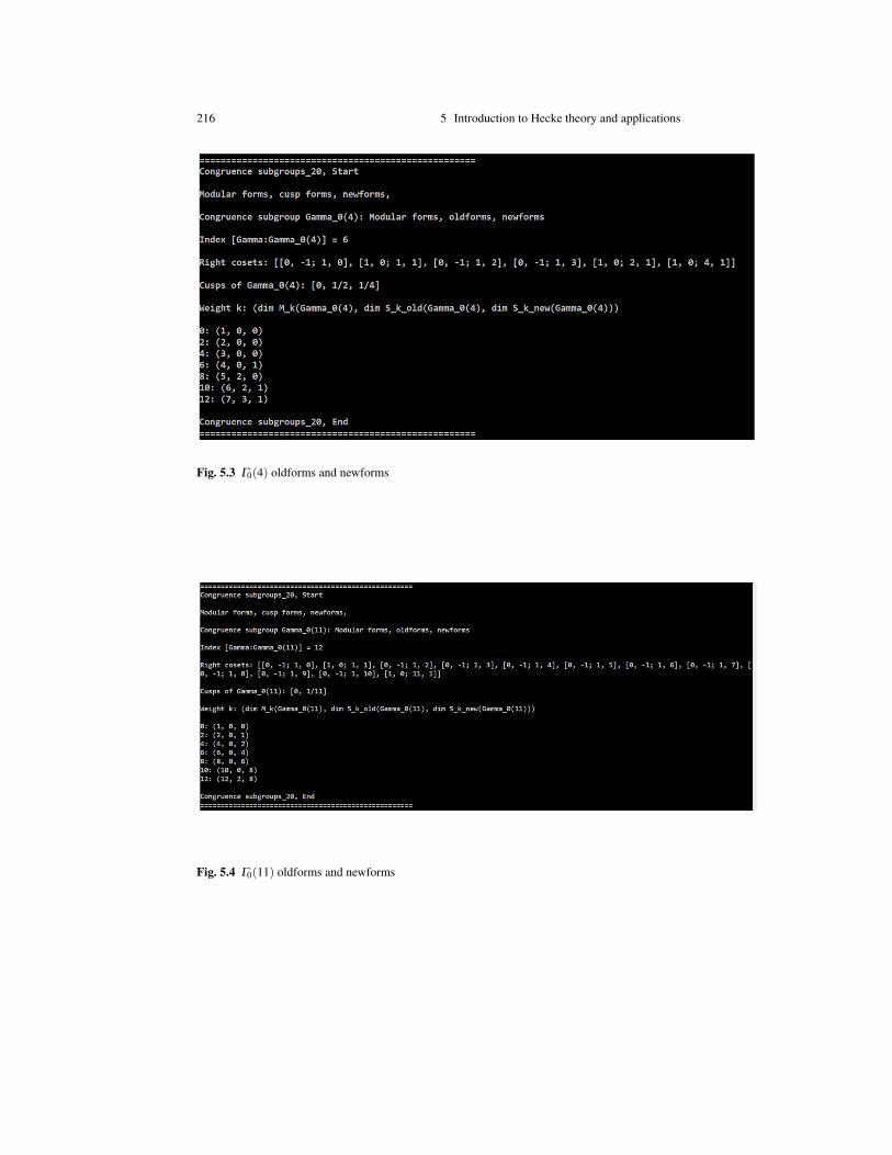
216 5 Introduction to Hecke theory and applications
Fig. 5.3 Γ0(4) oldforms and newforms
Fig. 5.4 Γ0(11) oldforms and newforms

5.3 Numerology: Lagrange, Jacobi, Ramanujan, Mordell 217
5.3 Numerology: Lagrange, Jacobi, Ramanujan, Mordell
The present section draws some conclusion from the existence of simultaneouseigenforms of the Hecke operators. First we prove a conjecture of Ramanujan con-cerning a certain numerical function. Secondly, we derive the four squares theorem.
Information about the Ramanujan τ-function is encoded by the modular discrim-inant, the cusp form ∆ ∈ S12(Γ ).
Definition 5.31 (Ramanujan τ-function). The Fourier coefficients (τn)n∈N of thenormalized discriminant form
∆(τ)
(2π)12 =∞
∑n=1
τn ·qn, q = e2πi·τ ,
define the Ramanujan τ-function
τ : N→ Z, n 7→ τ(n) := τn.
According to Proposition 3.14 all Fourier coefficients are integers τ(n) ∈ Z.
Computing the first coefficients τ(n) up to n = 6 gives
∆(τ)
(2π)12 = q−24q2 +252q3−1.472q4 +4.830q5−6.048q6 +O(7)
From these values one verifies at once the product formula
τ(2) · τ(3) =−24 ·252 =−6.048 = τ(6),
and as a particular case of the recursion formula
τ(p2) = τ(p)2− p11 · τ(p0)
the formula for p = 2
τ(22) =−1.472 = τ(2)2−211 = (−24)2−2.048.
From explicit computation of the first 30 values of τ(n) Ramanujan [45]conjectured in 1916 several generalizations. Figure 5.5 shows equations (103)and (104) from the original paper with two of Ramanujan’s conjectures.
Note. There is a typo in equation (104) referring to the factor 2. It should read
|τ(p)| ≤ 2 · p11/2

218 5 Introduction to Hecke theory and applications
Fig. 5.5 Ramanujan’s conjecture on τ(n) from [45]
The conjecture was proved inter alia one year later by Mordell [42]. Figure 5.6shows Mordell’s introduction from his paper.
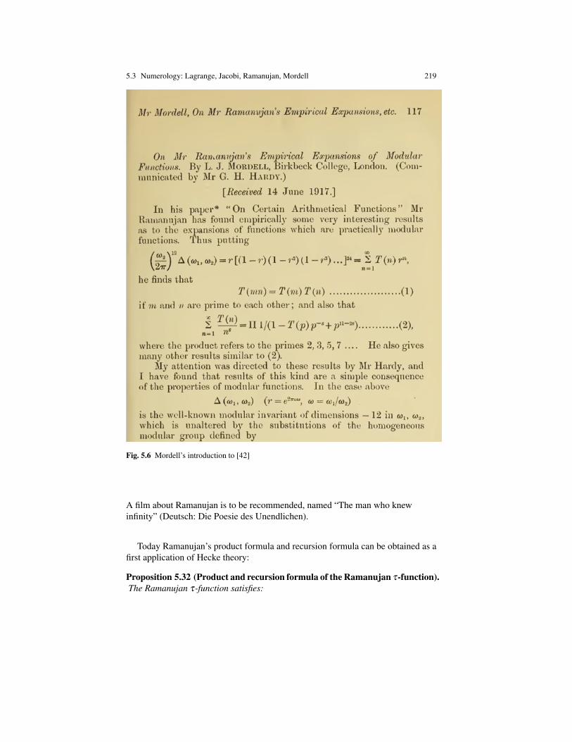
5.3 Numerology: Lagrange, Jacobi, Ramanujan, Mordell 219
Fig. 5.6 Mordell’s introduction to [42]
A film about Ramanujan is to be recommended, named “The man who knewinfinity” (Deutsch: Die Poesie des Unendlichen).
Today Ramanujan’s product formula and recursion formula can be obtained as afirst application of Hecke theory:
Proposition 5.32 (Product and recursion formula of the Ramanujan τ-function).The Ramanujan τ-function satisfies:

220 5 Introduction to Hecke theory and applications
1. Product formula: For all integers m,n≥ 1
τ(m) · τ(n) = ∑r|(m,n)
r11 · τ(mn/r2).
In particular, for coprime m and n:
τ(m) · τ(n) = τ(m ·n).
2. Recursion formula: For all primes p and integers k ≥ 1
τ(p) · τ(pk) = τ(pk+1)+ p11 · τ(pk−1).
Proof. 1. Consider an arbitrary, but fixed m ∈N. Corollary 5.13 from Hecke theoryderives the eigenvalue equation
Tm
(∆
(2π)12
)= τ(m) ·
∆
(2π)12
When equating for each fixed n ∈ N the terms of order n on both sides of theequation the coefficent formula from Theorem 5.11 implies:
∑r|(m,n)
r11 · τ(mn/r2) = τ(m) · τ(n).
For coprime integers m,n we have (m,n) = 1 and the summation reduces to thesingle term for r = 1:
τ(m) · τ(n) = τ(m ·n)
2. We set m = pk and n = p in the product formula from part 1). Due to
(pk, p) = p
we now have two summands, referring to the indices r = 1 and r = p. We obtain
τ(pk) · τ(p) = τ(pk+1)+ p11 · τ(pk−1), q.e.d.
Remark 5.33 (Growth estimation of the Ramanujan τ-function). The final conjec-ture of Ramanujan about the τ-function is the growth estimation
|τ(p)| ≤ 2 · p11/2, p prime,
see Figure 5.5 equation (104) (after correction). This conjecture lies much deeperthan Ramanujan’s other conjectures. Deligne proved the growth condition of the τ-functionas a consequence of his proof of the Weil conjectures in 1974.

5.3 Numerology: Lagrange, Jacobi, Ramanujan, Mordell 221
The next application uses information encoded by modular forms from M2(Γ0(4)).The “Four squares theorem” answers the question: How many possibilities exist torepresent a positive integer as the sum of four integer squares?
Fermat recalls in a letter to a friend from 1659 those results from arithmeticwhich he considers his most important contribution to this field. One of these resultsis the claim that any natural number can be written as the sum of four squares. Thefirst proof of this theorem has been given by Lagrange in 1770. The more refinedversion of Theorem 5.38 is due to Jacobi in 1834. For the history of these issuessee [47].
Definition 5.34 (Representing integers as sum of squares). The number of possi-bilities to represent a non-negative integer n as the sum of k integer squares definesthe arithmetic function
r : N∗×N∗→ N
withr(n,k) := card
v = (v1, ...,vk) ∈ Zk : n = v2
1 + ...+ v2k
.
Note that r(n,k) counts k-tuples with positive and negative components as dif-ferent, and distinguishes also k-tuples with the same components, but in differentorder.
We will see that the representation of integers as sum of squares is related to thecongruence subgroup Γ0(4), the relevant space of modular forms is M2(Γ0(4)).
Definition 5.35 (Generating function ϑ ). The series
ϑ(τ,k) :=∞
∑n=0
r(n,k) ·qn, q := e2πiτ ,
which is generated by the sequence r(n,k)n∈N, is named a ϑ -series.
Proposition 5.36 (Generating function as modular form). The generating function θ(−,4)is a modular form of weight 2 of the congruence subgroup Γ0(4), i.e.
θ(−,4) ∈M2(Γ0(4)).
Its Fourier series starts
θ(τ,4) = 1+8q+O(2), q = e2πiτ .

222 5 Introduction to Hecke theory and applications
Proof. Scetch, see cf. [17, Chap.1, §2; Chap. 4, §9], [36].
i) The congruence subgroup Γ0(4) is generated as
Γ0(4) =< T,γ >
with
γ =
(1 04 1
)∈ Γ0(4)
ii) The translation T apparently satisfies
ϑ(−,4)[T ]2 = ϑ(−,4)
The product formulaϑ(τ,4) = ϑ(τ)4
with
ϑ(τ) =∞
∑n=0
r(n,1) ·qn
reduces the weak modularity
ϑ(−,4)[γ]2 = ϑ(−,4)
to the transformation formula for ϑ : The difficult part is to prove
ϑ(−1/(4τ)) =√−2iτ ·ϑ(τ).
Then follows
ϑ
(τ
4τ +1
)= ϑ
(−1
4(−1/(4τ)−1)
)=
√√√√2i
(1
4τ+1
)·ϑ
(−
14τ−1
)=
=
√√√√2i
(1
4τ+1
)·ϑ
(−
14τ
)=
√√√√2i
(1
4τ+1
)· (−2iτ) ·ϑ(τ) =
√4τ +1 ·ϑ(τ),
and exponentionϑ(−,4) = ϑ
4
shows the transformation formula
ϑ
(τ
4τ +1,4
)= (4τ +1)2 ·ϑ(τ,4) i.e. ϑ(−,4)[γ]2 = ϑ(−,4)
iv) The Fourier series
ϑ(τ) = 1+ r(1,1) ·q+O(q2) = 1+2 ·q+O(q2)
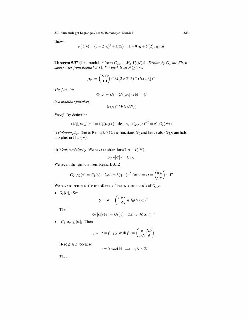
5.3 Numerology: Lagrange, Jacobi, Ramanujan, Mordell 223
showsϑ(τ,4) = (1+2 ·q)4 +O(2) = 1+8 ·q+O(2), q.e.d.
Theorem 5.37 (The modular form G2,N ∈M2(Γ0(N))). Denote by G2 the Eisen-stein series from Remark 3.12. For each level N ≥ 1 set
µN :=(
N 00 1
)∈M(2×2,Z)∩GL(2,Q)+
The functionG2,N := G2−G2[µN ]2 : H−→ C
is a modular functionG2,N ∈M2(Γ0(N))
Proof. By definition
(G2[µN ]2)(τ) := G2(µ2(τ)) ·det µN ·h(µN ,τ)−2 = N ·G2(Nτ)
i) Holomorphy: Due to Remark 3.12 the functions G2 and hence also G2,N are holo-morphic in H∪∞.
ii) Weak modularity: We have to show for all α ∈ Γ0(N):
G2,N [α]2 = G2,N .
We recall the formula from Remark 3.12
G2[γ]2(τ) = G2(τ)−2πi · c ·h(γ,τ)−2 for γ := α =
(a bc d
)∈ Γ
We have to compute the transforms of the two summands of G2,N .
• G2[α]2: Set
γ := α =
(a bc d
)∈ Γ0(N)⊂ Γ .
ThenG2[α]2(τ) = G2(τ)−2πi · c ·h(α,τ)−2
• (G2[µN ]2)[α]2: Then
µN ·α = β ·µN with β :=(
a Nbc/N d
)Here β ∈ Γ because
c≡ 0 mod N =⇒ c/N ∈ Z
Then

224 5 Introduction to Hecke theory and applications
(G2[β ]2)(z) = G2(z)−2πi · (c/N) ·h(β ,z)−2
Hence with the argument z = µN(τ) = Nτ
(G2[β ]2)(µN(τ)) = G2(µN(τ))−2πi · (c/N) ·h(β ,µN(τ))−2
Then
((G2[µN ]2)[α]2)(τ) = (G2[µN ·α]2)(τ) = (G2[β ·µN ]2)(τ) =
= ((G2[β ]2)[µN ]2)(τ) = (G2[β ]2)(µN(τ)) ·h(µN ,τ)−2 ·N =
=(G2(µN(τ))−2πi · (c/N) ·h(β ,µN(τ))
−2) ·h(µN ,τ)−2 ·N =
= G2(µN(τ)) ·h(µN ,τ)−1 ·N−2πi((c/N) ·N) · (h(β ,µN(τ)) ·h(µN ,τ))
−2 =
= (G2[µN ]2)(τ)−2πi((c/N) ·N) · (h(β ,µN(τ)) ·h(µN ,τ))−2
Now
h(β ,µN(τ)) = h(β ,Nτ) = (c/N) ·Nτ +d = cτ +d and h(µN ,τ) = 1
andh(α,τ) = cτ +d
which impliesh(β ,µN(τ)) = h(α,τ)
Hence((G2[µN ]2)[α]2)(τ) = (G2[µN ]2)(τ)−2πi · c ·h(α,τ)−2
As a consequence, the transformation formulas for both summands imply:
G2,N [α]2 = G2[α]2− ((G2[µN ]2)[α]2) = G2− (G2[µN ]2) = G2,N
iv) Finally one checks the Fourier expansion at the cusps using the Fourier expansionof G2 from Remark 3.12, see [17, Chap. I, Exerc. 1.2.8.e] and [33, Chap. IX, §3, Example 4],q.e.d.
Theorem 5.38 (Four squares theorem). For any n ∈ N, n≥ 1, there are
r(n,4) = 8 · ∑d|n, 4-d
d
possibilities to represent the non-negative integer n as the sum of 4 integer squares.In particular for 4 - n
r(n,4) = 8 ·σ1(n) = 8 ·∑d|n
d.
Proof. Computation within M2(Γ0(4)):

5.3 Numerology: Lagrange, Jacobi, Ramanujan, Mordell 225
i) Dimension: dim M2(Γ0(4)) = 2 according to Theorem 3.26, see also Figure 5.3.
ii) Basis: According to Theorem 5.37 for each N ≥ 2 the Eisenstein series
G2,N(τ) := G2(τ)−N ·G2(Nτ)
is a modular form of the congruence subgroup Γ0(N) of weight 2, i.e.
G2,N(τ) ∈M2(Γ0(N)).
The Fourier expansion of G2 from Remark 3.12 provides for the two Eisensteinseries G2,2 and G2,4 the Fourier expansions
G2,2(τ) =−π2
3
1+24 ·∞
∑n=1
∑d|n
d odd
d
qn
=−π2
3(1+24q+O(2))
and
G2,4(τ) =−π2
(1+8 ·
∞
∑n=1
(∑
d|n, 4-nd
)qn
)=−π
2(1+8q+O(2)).
Comparing terms of order 0 and 1 in the Fourier expansions shows that bothEisenstein series are linearly independent. Hence the family (G2,2,G2,4) is a basisof M2(Γ0(4)). In particular, it generates θ(−,4).
Proposition 5.36 implies by comparing Fourier coefficients of order 0 and 1
θ(−,4) =−1
π2 G2,4.
Equating on both sides the Fourier coefficients of order n ∈ N∗ shows
r(n,4) = 8 · ∑d|n, 4-d
d, q.e.d.
Example 5.39 (Modular forms via ϑ -functions). Figure 5.7 shows for some pairs (k,e)the numbers
r(n,k,e).
Here r(n,k,e) ∈ N is the number of different representations of n as a sum of ksummands, each an e-power. These numbers are the Fourier coefficients of suitablemodular forms. The case
r(n,4,2) =: r(n,4)
has been investigated in Theorem 5.38. The figure shows the output of the PARI-script Modular_forms_theta_01.

226 5 Introduction to Hecke theory and applications
Fig. 5.7 Modular functions to compute r(−,k,e)

Part IIAdvanced Theory


Chapter 6Application to imaginary quadratic fields
The modular j-invariant parametrizes the set of compex tori by the values of theaffine part of the modular curve X(Γ ) ' P. All complex analytic properties of agiven torus with normalized period lattice (1,τ) are encoded in the value j(τ) ∈ Cof the modular j-invariant. But j(τ) is too coarse to discriminate between the arith-metic properties of the members of a class of biholomorphic equivalent tori.
Section 6.2 will investigate for tori with complex multiplication: Which arith-metic information can be obtained when considering besides j(τ) also the values
j(α(τ)), α ∈ Γm,prim, m ∈ N∗?
References for the present chapter are [66, Chap. 6.1] and [50].
6.1 Imaginary quadratic fields and tori with complexmultiplication
As a first arithmetic property of complex tori and elliptic curves we observe: Com-plex tori with normalized lattice generated by (1,τ) relate for certain numbers τ ∈Hto an imaginary quadratic field. How to characterize tori with those arithmetic prop-erties? The answer is given by Theorem 6.6.
As a general reference for number fields we recommend [22], [40], [32].
Definition 6.1 (Number field).
229
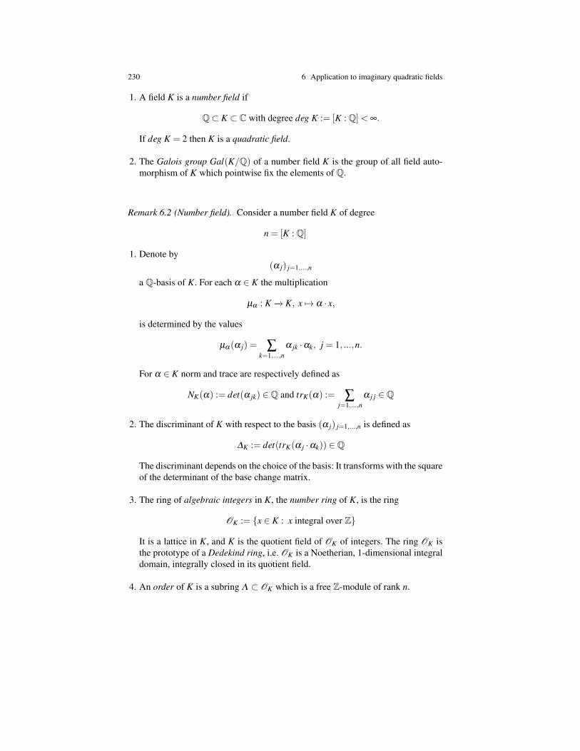
230 6 Application to imaginary quadratic fields
1. A field K is a number field if
Q⊂ K ⊂ C with degree deg K := [K : Q]< ∞.
If deg K = 2 then K is a quadratic field.
2. The Galois group Gal(K/Q) of a number field K is the group of all field auto-morphism of K which pointwise fix the elements of Q.
Remark 6.2 (Number field). Consider a number field K of degree
n = [K : Q]
1. Denote by(α j) j=1,...,n
a Q-basis of K. For each α ∈ K the multiplication
µα : K −→ K, x 7→ α · x,
is determined by the values
µα(α j) = ∑k=1,...,n
α jk ·αk, j = 1, ...,n.
For α ∈ K norm and trace are respectively defined as
NK(α) := det(α jk) ∈Q and trK(α) := ∑j=1,...,n
α j j ∈Q
2. The discriminant of K with respect to the basis (α j) j=1,...,n is defined as
∆K := det(trK(α j ·αk)) ∈Q
The discriminant depends on the choice of the basis: It transforms with the squareof the determinant of the base change matrix.
3. The ring of algebraic integers in K, the number ring of K, is the ring
OK := x ∈ K : x integral over Z
It is a lattice in K, and K is the quotient field of OK of integers. The ring OK isthe prototype of a Dedekind ring, i.e. OK is a Noetherian, 1-dimensional integraldomain, integrally closed in its quotient field.
4. An order of K is a subring Λ ⊂ OK which is a free Z-module of rank n.

6.1 Imaginary quadratic fields and tori with complex multiplication 231
5. The number field K has a Q-basis (α j) j=1,...,n by algebraic integers α j ∈ OK .Each element α ∈ K has a unique representation
α =Zα1 + ...+Zαn
∆K
6. For a quadratic field K =Q(√
d) with a squarefree integer d ∈ Z one has
∆K =
4 ·d if d ≡ 2,3 mod 4
d if d ≡ 1 mod 4
and
OK = Z
[∆K +
√∆K
2
]7. Each number field K has a primitive element, i.e.
K =Q(α)
with a suitable α ∈ K. Each primitive element satisfies a polynomial equation
P(α) = 0 with P(X) ∈Q[X ] and deg P = deg K.
8. Each quadratic number field has the form
K =Q(√
d) with d ∈ Z squarefree.
If d < 0 then K is named imaginary quadratic, if d > 0 then K is named realquadratic.
9. The Galois group Gal(K/Q) of a quadratic number field K =Q(√
d) equals thegroup Z2. Its generator
σ1 : K −→ K, z 7→ σ1(z),
satisfies
σ1(z) =
−z d > 0
z d < 0
Setσ0 := idGal(K/Q).
Then norm and trace of an element z ∈ K can be computed by using the elemen-tary symmetric functions:
N(z) = σ0(z) ·σ1(z) and Tr(z) = σ0(z)+σ1(z)

232 6 Application to imaginary quadratic fields
Note. Due to historical reasons the symbol O has two different meanings. In thecontext of complex analysis O also denotes the complex structure sheaf.
Definition 6.3 (Endomorphisms of a torus). An endomorphism f of a torus
(T,0) = C/Λ
is a holomorphic mapf : (T,0)−→ (T,0)
with f (0) = 0.
Recall from Proposition 2.3 that each endomorphism f of a torus fits into acommutative diagram
C C
C/Λ C/Λ
µα
p p
f
with a unique multiplication map µα determined by an element α = α f ∈ C: Forall z ∈ C
µα(z) = α · z
Proposition 6.4 (Endomorphism ring). The set of endomorphisms of a torus
T = C/Λ
constitutes with respect to addition and composition a ring End(T ), the endomor-phism ring of T . The map
End(T )−→ α ∈ C : α ·Λ ⊂Λ, f 7→ α f ,
is an isomorphism of rings.
If not stated otherwise by the above ring isomorphism we identify the endomor-phism ring End(T ) with a subring of C. Because each torus T is an Abelian groupits endomorphism ring End(T ) comprises at least the group Z:
Z⊂ End(T )⊂ C.
Which intermediate rings are possible? The case

6.1 Imaginary quadratic fields and tori with complex multiplication 233
End(T ) = Z
is the general case, justifying a specific name for tori with additional endomor-phisms.
Definition 6.5 (Complex multiplication (CM)).
1. A complex number τ ∈H is a CM-point and its class [τ] ∈ X(Γ ) in the modularcurve is a CM-class, if the corresponding torus
T = C/Λ , Λ = Z⊕Z · τ,
satisfiesZ ( End(T )
2. The values j(τ)⊂ C at CM-points τ ∈H are named singular moduli or singularvalues of the modular invariant j.
Theorem 6.6 states a remarkable relation between tori and number fields. It re-veals the arithmetic structure encoded in a complex torus with complex multiplica-tion.
Theorem 6.6 (Complex multiplication and imaginary quadratic fields). Con-sider a point τ ∈H.
1. Then: τ is a CM-point ⇐⇒ Q(τ) is an imaginary quadratic number field.
2. If τ is a CM-point with K :=Q(τ), then the torus
T := C/Λτ , Λτ := Z+Z · τ,
has as ring of endomorphisms
End(T )⊂ C
an order of K.
Note that any order of an imaginary quadratic number field is a lattice.
Proof. 1. i) Consider a CM-point τ ∈H. By definition exists α ∈ C\Z with
α ·Λτ ⊂Λτ .
We obtain a matrix
γ =
(a bc d
)∈M(2×2,Z)
with
α ·(
1τ
)= γ ·
(1τ
).

234 6 Application to imaginary quadratic fields
We obtainα = a+b · τ, α · τ = c+d · τ,
which implies b 6= 0, because α /∈ Z, and
b · τ2 +(a−d) · τ− c = 0.
Because τ ∈H is not a real number, the number field Q(τ) is imaginary quadratic.
ii) Assume that τ ∈H belongs to an imaginary quadratic number field. Then forsuitable integers a,b,c ∈ Z with a 6= 0 because τ ∈H
a · τ2 +b · τ + c = 0.
From
(aτ) ·(
1τ
)=
(0 a−c −b
)·(
1τ
)follows aτ ∈ End(T ), ατ /∈ Z, and T has complex multiplication,
2. Assume that T has complex multiplication and consider an endomorphism f ∈ End(T )operating as multiplication µα with a complex number α . Alike to the proof ofpart 1, i) we obtain a matrix
γ =
(a bc d
)∈M(2×2,Z)
with
α ·(
1τ
)= γ ·
(1τ
)Therefore α is an eigenvalue of γ and satisfies the eigenvalue equation, which isan integral equation:
α2− (d +a) ·α +ab− cd = 0.
As a consequence α ∈ OK , which implies
Z ( End(T )⊂ OK
Because OK is free of rank = 2 the same holds true for End(T ), and thesubring End(T ) is a sublattice of OK , i.e. an order, q.e.d.
We consider in detail the two elliptic points of the modular group Γ , seeTheorem 2.16:
Example 6.7 (CM-points).
1. Elliptic point i: The point i ∈ H determines the normalized lattice of Gaussianintegers

6.1 Imaginary quadratic fields and tori with complex multiplication 235
Λi = Z+Z · i
The torus T = C/Λi has the endomorphism ring
End(T ) = Λi
The endomorphism ringEnd(T ) = Λi
equals the ringOK ⊂ K :=Q(i) =Q(
√−1)
of algebraic integers from K. Recall from Corollary 3.21
j(i) = 1728 = 26 ·33 ∈ Z.
2. Elliptic point ρ = e2πi/3: The point ρ ∈H determines the normalized lattice
Λρ = Z+Z ·ρ
The torus T = C/Λρ has the endomorphism ring
End(T ) = Λρ
The result is similar to the first example: The endomorphism ring
End(T ) = Λρ
equals the ringOK ⊂ K :=Q(ρ) =Q(
√−3)
of algebraic integers from K. Recall from Corollary 3.21
j(ρ) = 0 ∈ Z.
Also the element 2ρ ∈H belongs to K. The torus
T = C/Λ2ρ
with the normalized lattice
Λ2ρ = Z+Z ·2ρ
has as endomorphisms the multiplication with arbitrary elements
α ∈Λ2ρ .
For the proof one uses the equation
ρ2 +ρ +1 = 0.

236 6 Application to imaginary quadratic fields
The endomorphism ring isEnd(T ) = O
withO = Λ2ρ ( OK
is a proper order of K. Note j(ρ) = 0 ∈ Z. A PARI-calculation shows
j(2ρ) = 54000 ∈ Z.
6.2 Modular polynomials
The present section takes up the study of imaginary quadratic fields K from the view-point of modular forms. We relate complex multiplication to the value attainment ofthe modular j-function: Theorem 6.14 proves that the value j(τ)∈C is an algebraicinteger for any CM-class [τ] ∈ X(Γ ). The main tool to derive the necessary proper-ties of the modular j-invariant are the modular polynomials from Definition 6.8.
The modular polynomials are a family of polynomials (Fm(X))m∈N∗ which extractthe properties of the j-invariant j ∈M (H) from its transformation behaviour withrespect to the operation of the modular group Γ
Γ ×Γm,prim −→ Γm,prim
on the set of primitive matrices Γm,prim.
There is the following analogy to the family of Hecke operators (Tm)m∈N∗ : Thelatter extract the Fourier coefficients of a given modular f ∈Mk(Γ ) from thetransformation behaviour of f with respect to the operation of the modular group Γ
Γ ×Γm −→ Γm
on the set of matrices Γm. The Hecke operators are the family of linear maps with
Tm( f ) := ∑M∈V (m)
f [M]k
defined as the weighted sum of over a complete system V (m) of representatives.
Similarly the modular polynomials are the family
Fm(X) = ∏M∈V (m,prim)
(X− j M) ∈M (H)[X ]

6.2 Modular polynomials 237
defined as the product over a complete set V (m, prim) of representatives. Note thesimilarity between the definition f [M]k for modular forms from Definition 3.4 andthe expression j M for the automorphic function j.
We take up the investigation of the integral matrices Γm from Section 5.1, inparticular Definition 5.4 of the set Γm,prim of primitive matrices and its completeset V (m, prim) of representatives with respect to the canonical left Γ -operation.The set V (m, prim) has cardinality
ψ(m) := m · ∏p|m
p prime
(1+(1/p))
Definition 6.8 (Modular polynomials). Consider m∈N∗ and the complete set V (m, prim)of representatives of Γ \Γm,prim.
1. Each matrix M ∈V (m, prim) induces the automorphism of the upper half-plane
M : H→H, τ 7→Mµ(τ).
The ψ(m) functionsjM := j M ∈V (m, prim)
are the class invariants of Γ \Γm.
2. The m-th modular polynomial is the polynomial
Fm(X) := ∏M∈V (m,prim)
(X− jM) ∈M (H)[X ].
Note. The modular invariant is constant along the orbits of the action of themodular group Γ . Therefore the value of jM in Definition 6.8 does not dependon representing a coset from Γ \Γm,prim by the matrix M ∈ V (m, prim) or by thematrix γ ·M,γ ∈ Γ .
Example 6.9 (Modular polynomials). The PARI-script modular_polynomial_01computes for several m the modular polynomials Fm, see Figure 6.1.

238 6 Application to imaginary quadratic fields
Fig. 6.1 Modular polynomials
1. m = 2:ψ(2) = 3
andF2(X , j) = X3+
+(− j2 +1488∗ j−162000)∗X2+
+(1488∗ j2 +40773375∗ j+8748000000)∗X+
+( j3−162000∗ j2 +8748000000∗ j−157464000000000)
2. m = 3:ψ(3) = 4
andF3(X , j) = X4+
+(− j3 +2232∗ j2−1069956∗ j+36864000)∗X3+
+(2232∗ j3+2587918086∗ j2+8900222976000∗ j+452984832000000)∗X2+
+(−1069956∗ j3+8900222976000∗ j2−770845966336000000∗ j+1855425871872000000000)∗X+
+( j4+36864000∗ j3+452984832000000∗ j2+1855425871872000000000∗ j)
The roots of the modular polynomial Fm(X) ∈M (H)[X ] are exactly the classinvariants jM ∈V (m, prim) of the operation
Γ ×Γm,prim −→ Γm,prim
We denote by sµ , j = 1, ...,ψ(m), the elementary symmetric functions in ψ(m)variables. Then up to sign the functions
sµ( j1, ..., jψ(m)) ∈M (H), j = 1, ...,ψ(m),
are the coefficients of the modular polynomial Fm(X). E.g.,
6.2 Modular polynomials 239
(−1)ψ(m)sψ(m)( j1, ..., jψ(m)) = (−1)ψ(m) · j1 · ... · jψ(m)
is the constant term and
(−1) ·σ1( j1, ..., jψ(m)) =−( j1 + ...+ jψ(m))
is the coefficient of the term Xψ(m)−1. Theorem 6.10 now takes a closer look onthese coefficients and proves: They are polynomials in the modular j-invariant withinteger coeffcients, i.e. the coefficients belong to the subring
Z[ j]⊂M (H).
See also Example 6.9.
Theorem 6.10 (Coefficients of the modular polynomials). For each m ∈ N∗
Fm(X) = ∏M∈V (m,prim)
(X− jM) ∈ Z[ j][X ] = Z[ j,X ].
Proof. For arbitrary but fixed index µ = 1, ...,ψ(m) we consider the coefficient
c := cµ := σµ( j1, ..., jψ(m)) ∈M (H)
of the modular polynomial
Fm(X) ∈M (H)[X ].
We prove step by step the following properties of the coefficient c ∈M (H) untilarriving at c ∈ Z:
i) Weakly modular: According to Corollary 5.7 right multiplication with anelement γ ∈ Γ permutes the orbits of the Γ -left operation Φm
[M1], ..., [Mψ(m)]= [M1 · γ], ..., [Mψ(m) · γ].
Hence right multiplication does not change the value of the elementary symmetricfunctions: For all j = 1, ...,ψ(m)
σµ( j1, ..., jψ(m)) = σµ( j1 γ, ..., jψ(m) γ).
Therefore c is weakly modular.
ii) Holomorphic on H: The j-invariant is holomorphic on H according toCorollary 3.16. Therefore also the coefficient c is holomorphic.
iii) Meromorphic at ∞: The coefficient c is weakly modular according to part i).Hence c has a Fourier expansion

240 6 Application to imaginary quadratic fields
c(τ) = ∑ν∈Z
aν ·qν , q = e2πiτ .
We have to show that the singularity q = 0 is a pole of c. For the proof we estimatethe growth of c: According to Corollary 3.21 the modular invariant has the Fourierexpansion
j(τ) =1q+P(q)
with P ∈ Zq a convergent power series with integer coefficients. For an uppertriangular matrix
α =
(a b0 d
)∈V (m, prim)
the Fourier series of the class invariant j α derives from the Fourier series of j bysubstituting the variable q = e2πiτ by
e2πiα(τ) = e2πi(b/d) ·q(a/d)
The equalityad = m
impliese2πiα(τ) = ζ
abm · (q1/m)a2
with ζm := e2πi/m
a primitive m-th root of unity. In particular
|( j α)(τ)| ≤1|q|a/d +O(1)
for a single class invariant. Hence for suitable constants k,M
|c(τ)| ≤M ·1|q|k
for small q ∈ ∆ \0.
iv) Integrality c ∈ OK [ j]: Due to the part already proved, Corollary 3.22 impliesthat c is a polynomial with complex coefficients in the modular invariant, i.e.
c ∈ C[ j].
We show that evenc ∈ OK [ j]
withK :=Q(ζm)
the m-th cyclotomic number field. For the proof we recall from part iii) the substi-tution of q by

6.2 Modular polynomials 241
ζmab · (q1/m)a2
.
As a consequence the class invariant j α has a Fourier expansion with respectto q1/m, namely
j(α(τ)) =1
(q1/m)a2 ·ζmab +P
((q1/m)a2 ·ζm
ab),
which shows that the Fourier coefficents of c belong to K. According to Corollary 3.22the coefficients of the polynomial c ∈ C[ j] are Z-linear combinations of the Fouriercoefficients of c. Hence the coefficients are Z-linear combinations of the m-th rootsof unity. Therefore the coefficients of c ∈ C[ j] are algebraic integers from OK ,i.e. c ∈ OK [ j].
v) Integrality c ∈ Z[ j]: The operation of the Galois group
Gal(K/Q)' (Z/mZ)∗.
extends to an operation on the set j1, ..., jψ(m) of class invariants
Gal(K/Q)× j1, ..., jψ(m)→ j1, ..., jψ(m), (χ, jµ) 7→ jµχ ,
which is defined as follows: Assume χ ∈Gal(K/Q) maps χ(ζm)= ζme with (e,m) = 1.
If jµ is the class invariant of the matrix
M =
(a b0 d
)then we define jµ
χ as the class invariant of the matrix
Mχ =
(a bχ
0 d
)with
0≤ bχ < d and bχ ≡ e ·b mod d.
Because the function c is fixed under the operation of Gal(K/Q), its Fourier co-efficients belong to the fixed field Q. Due to part iv) the Fourier coefficients evenbelong to
Q∩OK = Z, q.e.d.
We now evaluate the modular polynomials
Fm(X) ∈ Z[ j][X ]
on the diagonal X = j, i.e. we consider the polynomials of the single variable j

242 6 Application to imaginary quadratic fields
Φm( j) := Fm( j, j) = ∏M∈V (m,prim)
( j− jM) ∈ Z[ j].
Example 6.11 (The polynomials Φm( j) ∈ Z[ j]). We take up Example 6.9 with Figure 6.2,which shows some polynomials Φm. The PARI script Modular_polynomial_02computes their factorization:
1. m = 2:
Φ2( j)=F2( j, j)=− j4+2978∗ j3+40449375∗ j2+17496000000∗ j−157464000000000
splits into the factors
j−8000, j−1728, ( j+3375)2
2. m = 3:
Φ3( j) = F3( j, j) =− j6 +4464∗ j5 +2585778176∗ j4 +17800519680000∗ j3
−769939996672000000∗ j2 +3710851743744000000000∗ j
splits into the factors
j−54000, ( j−8000)2, j, ( j+32768)2
3. The example Φ5( j) shows: In general Φm( j), m prime, does not split into linearfactors over Z.
Fig. 6.2 Some polynomials Φm and their factorization

6.2 Modular polynomials 243
Lemma 6.12 (Leading coefficient of the modular polynomials). For squarefree m≥ 2the polynomial
Φm( j) ∈ Z[ j]
has leading coefficient ±1.
Example 6.9 illustrates Lemma 6.12 by
Φ2( j) =− j4 +O(3), Φ3( j) =− j6 +O(5) and Φ7( j) =− j10 +O(9).
Proof. The functionΦm( j) : H−→ C
is an automorphic function. Consider its Fourier expansion
Φm( j)(τ) =ck
qk +ck−1
qk−1 + higher terms
Because j has a pole at τ = ∞ of order = 1, the coefficient ck of the Fourier series isalso the leading coefficient of Φm as polynomial in j. The coefficient is the productof the highest negative coefficients of the factors
j− jµ , µ = 1, ...,ψ(m).
For arbitrary but fixed µ the representation
j(τ) =1q+P(q)
implies
jµ(τ) = j
(aτ +b
d
)=
e−2πi(b/d)
qa/d +P(
qa/d · e2πi(b/d))
with jµ corresponding to the matrix(a b0 d
)∈V (m, prim).
Hence the highest negative coefficient in the Fourier expansion of j− jµ is1 a < de−2πi(b/d) a > d
Note that the case a = d is excluded because m = a ·d is squarefree. In any case thehighest negative coefficent of
j− jµ
is a root of unity, and the same holds for the coefficient ck of the product

244 6 Application to imaginary quadratic fields
Φ = ∏M∈V (m,prim)
( j− jM).
Because ck ∈ Z we have ck =±1, q.e.d.
According to Theorem 6.10 the modular polynomial
Fm( j,X) := Fm(X) =ψ(m)
∏µ=1
(X− jµ) ∈ Z[ j,X ]
is a polynomial in the two variables j and X with integer coefficients. It expands as
Fm( j,X) =N
∑n=0
(∑
r+s=ncrs · jr ·X s
), crs ∈ Z.
Proposition 6.13 will show that Fm( j,X) is symmetric in both variables, i.e. thecoefficients satisfy
crs = csr.
As a consequence, the highest exponent of j in Fm( j,X) is ψ(m).
Proposition 6.13 (Symmetry of the modular polynomials). The modular polyno-mials
Fm( j,X) ∈ Z[ j,X ], m ∈ N∗,
are symmetric with respect to j and X, i.e.
Fm( j,X) = Fm(X , j).
Proof. We set R = Z[ j] with quotient field
K := Q(R) =Q( j).
i) Irreducibility of Fm(X) ∈ R[X ] over K: The modular polynomial
Fm(X) = ∏M∈V (m,prim)
(X− jM) ∈ R[X ]
has as roots the class invariants
jM ∈V (m, prim) = j1, ..., jψ(m).
They are pairwise distinct which can be shown by comparing their Fourier coeffi-cients. To prove that Fm(X) is an irreducible polynomial we show that the Galoisgroup
Gal(L/K)

6.2 Modular polynomials 245
of the splitting fieldL = K( j1, ..., jψ(m))
of the polynomial Fm(X) ∈ R[X ] acts transitively on the roots. Then no root belongsto the fixed field K.
Elements of the Galois group can be obtained as follows: Any matrix γ ∈ Γ definesthe automorphism
L = K( j1, ..., jψ(m))−→ L, f 7→ f γ.
Consider two class invariants
jµ , jν , 1≤ µ,ν ≤ ψ(m)
corresponding to the matrices
Mµ ,Mν ∈V (m, prim)
One has to find γ ∈ Γ such that
jν = jµ γ
i.e. one has to find γ,γ ′ ∈ Γ such that
γ′ ·Mν = Mµ · γ,
which is achieved by Proposition 5.9, part 2). Therefore Gal(L/K) operates transi-tively on the roots of Fm(X), and the latter polynomial is irreducible over K.
ii) Common root of Fm( j,X) and Fm(X , j): We consider the two polynomials
f (X) := Fm( j,X) ∈ R[X ] and g(X) := Fm(X , j) ∈ R[X ]
For any matrix M ∈V (m, prim) the class invariant
jM := j M
is a root of the modular polynomial f (X) ∈ R[X ]. In particular for
α :=(
1 00 m
)∈Vm,prim
holds for all τ ∈H
0 = f ( jα(τ)) = Fm( j(τ), jα(τ)) = Fm
(j(τ), j
(τ
m
))

246 6 Application to imaginary quadratic fields
Replacing the argument τ by τ ·m shows for all τ ∈H
0 = Fm( j(τ ·m), j(τ)) = Fm( jβ (τ), j(τ)) = g( jβ (τ)) i.e. g( jβ ) = 0
with
β :=(
m 00 1
)∈Vm,prim
Also f ( jβ ) = 0 because β ∈Vm,prim. Hence both polynomials f (X),g(X) ∈ R[X ]have the common root jβ .
iii) Symmetry: Due to Lemma 6.12 and part i) the polynomial f (X) ∈ K[X ] isirreducible with leading coefficient ±1. Hence f (X) is the minimal polynomial ofthe field extension K ⊂ K[ jβ ], and g(X) is a multiple of f (X), i.e.
g(X) = h(X) · f (X)
with a polynomial h(X) ∈ K[X ]. According to Theorem 6.10 both polynomialsf (X) and g(X) have their coefficients already in the ring R = Z[ j]. The ring R isfactorial as a ring of polynomials over the factorial ring Z. The Lemma of Gaussimplies that also the polynomial h[X ] has all coefficients from R, and the equation
g(X) = h(X) · f (X)
holds in R[X ]. SetH( j,X) := h(X) ∈ R[X ] = Z[ j][X ].
ThenFm(X , j) = H( j,X) ·Fm( j,X) ∈ Z[ j,X ].
Considered as an equation in the ring Z[ j,X ] of polynomials in two variables thelast equation is invariant when interchanging the role of j and X . Hence also
Fm( j,X) = H(X , j) ·Fm(X , j) ∈ Z[ j,X ].
As a consequence
Fm( j,X) = H(X , j) ·H( j,X) ·Fm( j,X),
H(X , j) ·H( j,X) = 1,
andH(X , j) = H( j,X) =±1.
In case H(X , j) =−1 the previous equation
Fm( j,X) = H(X , j) ·Fm(X , j)
would imply
Fm(X , j) =−Fm( j,X) and Fm( j, j) =−Fm( j, j).

6.2 Modular polynomials 247
ThenFm( j, j) = 0
which contradicts the fact that Φm( j) = Fm( j, j) has leading coefficient ±1 accord-ing to Lemma 6.12. Therefore
H(X , j) = 1
andFm( j,X) = Fm(X , j), q.e.d.
We now derive from the theory of modular polynomials that all singular valuesj(τ) are algebraic integers.
Theorem 6.14 (Singular values of the modular j-invariant). For each CM-point τ ∈Hthe j-value j(τ) ∈ C is an algebraic integer. More precisely: There exists m ∈ N∗such that j(τ) is a root of the polynomial Φm(X) ∈ Z[X ].
Proof. Consider a CM-point τ ∈H. Theorem 6.6 implies that τ belongs to an imag-inary quadratic field
K =Q(√
d)
with d ∈ Z, d < 0 squarefree. The subring
OK ⊂ K
of algebraic integers of K is a free Z-module of rank = 2
OK = Z⊕Z · z
with a Z-basis (z,1), z ∈H. For admissible values of z see Remark 6.2.
i) A matrix α ∈ Γm,prim which fixes z: If a matrix α ∈ Γm,prim fixes a point τ ∈H, i.e.if
α(τ) = τ,
thenj(τ) = j(α(τ))
and vice versa. Hence the fixed points of the matrices α ∈ Γm,prim correspond to theroots of the polynomial Φm(X) ∈ Z[X ]. We determine a matrix α ∈ Γm,prim whichfixes z: The element
ξ :=
√
d d <−1
1+ i d =−1
is an algebraic integer. Its norm

248 6 Application to imaginary quadratic fields
N(ξ ) = ξ ξ ∈ Z
is squarefree. Multiplication with ξ ∈ OK defines a Z-linear endomorphism
OK −→ OK , x 7→ ξ · x.
Denote by
α =
(a bc d
)∈M(2×2,Z)∩GL(2,R)+
its matrix with respect to the basis (z,1) of OK . Then
ξ ·(
z1
)= α ·
(z1
)or in components (
ξ · zξ ·1
)=
(az+bcz+d
)• The first form shows: The matrix
α ∈M(2×2,Z)
which represents the Z-linear multiplication by ξ has the eigenvalue ξ and byconjugation α = α also the eigenvalue ξ . Hence
m := det α = ξ ξ = N(ξ ) ∈ Z
is squarefree which implies(a,b,c,d) = 1
and thereforeα ∈ Γm,prim
due to Definition 5.4.
• The component form shows: Considered as a fractional linear transformation
H−→H, w 7→ α(w) :=a ·w+bc ·w+d
the matrix matrix α ∈ GL(2,R)+ satisfies
α(z) =a · z+bc · z+d
=ξ · zξ ·1
= z
ii) j(z) is an algebraic integer: Lemma 5.6 implies the existence of a matrix
αµ ∈V (m, prim), µ ∈ 1, ...,ψ(m),
6.2 Modular polynomials 249
with the same Γ -orbit as α with respect to the left action
Φm,prim : Γ ×Γm,prim −→ Γm,prim, (A,M) 7→ A ·M,
w.l.o.g. µ = 1. Thenj α = j α1
because the value of j is constant along each orbit of the Γ -operation. Due to part i)
j(z) = j(α(z)) = j(α1(z)) = j1(z),
which implies: The function
Φm( j) = ∏M∈V (m,prim)
( j− jM) ∈ Z[ j]
vanishes at z ∈H:Φm( j)(z) = Φm( j(z)) = 0.
The polynomialΦm( j) ∈ Z[ j]
has integer coefficients, and leading coefficient ±1 due to Lemma 6.12. Hence
0 = Φm( j(z))
proves that j(z) is an algebraic integer. Hence the subring
Z[ j(z)]⊂ C
is integral over the ring Z.
iii) j(τ) is integral over Z[ j(z)]: The given element
τ ∈ K =Q+Q · z
has a representation
τ = β (z) :=az+b
dwith a primitive matrix
β =
(a b0 d
)∈ Γm,prim, m := a ·d.
Alike to the argument from part ii) the Γ -orbit of β passes through a matrix αµ ∈V (m, prim)which proves
j(τ) = j(β (z)) = j(αµ(z)) = jµ(z).
Theorem 6.10 implies that jµ is integral over the ring Z[ j]. Hence

250 6 Application to imaginary quadratic fields
j(τ) = jµ(z)
is integral over Z[ j(z)].
iv) j(τ) is an algebraic integer: When combining part iii) and part ii) thetransitivity of integral dependence proves the integrality of j(τ) over Z, i.e. τ is analgebraic integer, q.e.d.
Example 6.15 (Singular values of the modular j-function). Continuing Example 6.11we consider a CM-class [τ] ∈ X(Γ ) and choose the level
m = 2.
1. According to Example 6.11 the polynomial
Φ2( j) ∈ Z[ j]
has degree = 4 and factorizes as
j−8000, j−1728, ( j+3375)2
Which property is expressed by the three factors, why are the values j∈8000, 1728, −3375related?
According to Theorem 6.14 we determine a complete set of representatives
α j ∈ Γ2,prim, j = 1,2,3,
with fixed points α j(z j) = z j, z j ∈H:
•
α1 =
(1 −21 0
)has fixed point z1 =
1+ i√
72
which defines the lattice
Λ1 :=< 1,1+√−7
2>= OK1 ⊂ K1 :=Q(
√−7)
of the torus T1 := C/Λ1.
•α2 =
(1 1−1 1
)has fixed point z2 = i
which defines the lattice

6.3 Fractional ideals and the class number formula 251
Λ2 :=< 1, i >= OK2 ⊂ K2 :=Q(√−1)
of the torus T2 := C/Λ2.
•α3 =
(0 −12 0
)has fixed point z3 = i
√2
which defines the lattice
Λ3 :=< 1, i√
2 >= OK3 ⊂ K3 :=Q(√−2)
of the torus T3 := C/Λ3.
Hence the three resulting fields K j, j = 1,2,3 are imaginary quadratic. Due toTheorem 6.6 each of the three fields relates to a torus with complex multiplica-tion. In addition Theorem 6.14 shows that the tori have their j-values from
8000,1728,−3375
We already know j(z2) = j(i) = 1728. A PARI-computation completes at oncethe remaining values
j(z1) =−3375 and j(z3) = 8000.
One knows that all three fields have class number hK = 1, which will confirmCorollary 6.23.
6.3 Fractional ideals and the class number formula
A further application of the modular j-invariant to number theory is the class num-ber formula for imaginary quadratic fields.
We first recall the divisor sequence of a Riemann surface, e.g., cf. [63].
Remark 6.16 (Class group of a compact Riemann surface). The divisor sequenceon a compact Riemann surface X
1−→ O∗ −→M ∗ −→D −→ 0
provides the exact sequence of Abelian groups
1→ C∗→M ∗(X)→ Div(X)→Cl(X)→ 0.
because

252 6 Application to imaginary quadratic fields
H0(X ,O∗)=C∗, H0(X ,D)=Div(X), Cl(X) :=Div(X)
im[M ∗(X)→ Div(X)]and H1(X ,M ∗)= 0
The vanishing H1(X ,M ∗) = 0 is a result from the theory of compact Riemannsurfaces. It implies the isomorphy
Cl(X)'−→ H1(X ,O∗) = Pic(X)
between the group of divisor classes and the Picard group of isomorphism classesof holomorphic line bundles on X .
For number fields an analogue of divisors are fractional ideals, see [4, Chap. 9].
Definition 6.17 (Fractional ideal). Consider a number field K of degree.
1. A fractional ideal of K is defined as an OK-submodule a ⊂ K for which thereexists an element d ∈ OK , d 6= 0, with
d ·a⊂ OK .
Hence a fractional ideal is a subset of the form
a=ad⊂ K
with an ideal a⊂ OK . The element d is named a common denominator of a.
2. Fractional ideals generated by a single element α ∈ K
a= (α) := OK ·α
are named principal fractional ideals.
3. For two fractionals ideals a, b⊂ K the product
a ·b
is the fractional ideal generated by all products a ·b, a ∈ a, b ∈ b.
4. For a fractional ideal a 6= 0 the set
a−1 := x ∈ K : x ·a⊂OK
is named the inverse of a.
Remark 6.18 (Fractional ideals). Consider a number field K with number ring OK .

6.3 Fractional ideals and the class number formula 253
1. Each non-zero ideal of OK and each non-zero fractional ideal of K is a lat-tice of rank = deg K. The fractional ideals of K are the finitely generated OK-submodules of K.
2. Because OK is a Dedekind ring for a fractional ideal
a 6= 0 ⊂ K
the inverse a−1 is also a fractional ideal, see [4, Theor. 9.8]. It satisfies
a ·a−1 = (1)
3. With respect to multiplication the set of fractional ideals is an Abelian group J(K).Its quotient by the subgroup of principal fractional ideals is named the ideal classgroup or simply class group of K
Cl(K) := J(K)/im[K∗ −→ J(K)]
The canonical map isK∗ −→ J(K), x 7→ (x).
Hence two fractional idealsa1, a2 ∈ J(K)
define the same class in Cl(K) iff
a2 = a ·a1 for a suitable a ∈ K∗.
As a consequence there is an exact sequence of multiplicative Abelian groups
1−→ O∗K −→ K∗ −→ J(K)−→Cl(K)−→ 1
4. A number ring OK is a principal ideal domain iff
hK = 1
A theorem from algebraic number theory states the finiteness of the class number
hK := ord Cl(K)
see [40, Chap. 5, Cor. 2], [32, Chap. 12, §2]. The result is an analogue to the factthat the Neron-Severi group
NS(X) := Pic(X)/Pic0(X)
of a compact Riemann surface is finitely generated. This similarity strongly val-idates the analogy between the function fields of compact Riemann surfaces andnumber fields.

254 6 Application to imaginary quadratic fields
5. Comparing the exact sequence of a number field with the exact divisor sequenceof a Riemann surface from Remark 6.16 one easily observes the analogy betweencorresponding objects:
Compact Riemann surface X Number field KO∗X O∗KM ∗
X K∗
Div(X) J(K)
Cl(X) Cl(K)
Example 6.19 (Class number).
1. There are exactly 9 imaginary quadratic fields
K =Q(√−D), D > 0 squarefree integer,
with class number hK = 1. They belong to the values
D ∈ 1,2,3,7,11,19,43,67,163.
2. The imaginary quadratic field
K =Q(√−5)
has class number hK = 2. The class of the ideal
(2,1+√−5)⊂ OK
is not principal. It generates Cl(K), see [40, Chap. 5].
We now consider isomorphism classes of tori with complex multiplication and agiven number ring OK . How many isomorphism classes have OK as ring of endo-morphisms? Proposition 6.20 shows that their number equals the class number hK .In particular, there are only finitely many isomorphism classes of tori with endo-morphism ring OK .
Proposition 6.20 (Class group and tori with given endomorphism ring). Con-sider an arbitrary, but fixed imaginary quadratic field K with ring of integers OK .There exists a bijection
Cl(K)'−→ [T ] : T torus with End(T ) = OK
between the ideal class group Cl(K) and the set of classes of biholomorphicallyequivalent complex tori with ring of endomorphisms OK . The bijection is inducedby the attachement

6.3 Fractional ideals and the class number formula 255
normalized lattice Λ ∈ J(K) 7→ T = C/Λ with End(T ) = OK .
Its inverse is induced by the attachement
normalized torus T = C/Λ with End(T ) = OK 7→Λ ∈ J(K).
Proof. i) Well-definedness of the map: Starting with a fractional ideal
Λ ⊂ K ⊂ C
we may assumeΛ = Z+Z ·ω
a normalized lattice because the ideal class is determined up to an element of K.Due to Proposition 6.4 the torus
T := C/Λ
has the endomorphism ring
End(T ) = α ∈ C : α ·Λ ⊂Λ
Because Λ is an OK-module one obtains
OK ⊂ End(T ).
For the opposite inclusion consider a number α ∈ End(T ), i.e. α ·Λ ⊂ Λ . Thenormalization Z+Z · τ = Λ implies
α ·1 = α ∈Λ .
ii) Well-definedness of the inverse map: Starting with a normalized torus
T = C/Λτ , Λτ = Z+Z · τ, with End(T ) = OK
we have to show that Λτ ⊂ K is a fractional ideal. After choosing a Z-basis (1,ω)of OK the assumption
OK = End(T ) = α ∈ C : α ·Λτ ⊂Λτ
provides a matrix (a bc d
)∈M(2×2,Z)
with
ω ·(
1τ
)=
(a bc d
)·(
1τ
).
Henceω = a+b · τ and ω · τ = c+d · τ

256 6 Application to imaginary quadratic fields
• The second equation implies
τ =c
ω−α,
hence Λτ ⊂ Q(OK) = K.
• The lattice Λτ ⊂K is an OK-module because both equations taken together imply
1,ω,τ,τ ·ω ∈Λτ
• Finally the first equation implies
b ·Λτ ⊂ Z+Z ·b · τ ⊂ Z+Z ·ω = OK
As a consequence Λτ ⊂ K is a fractional ideal of K.
iii) The two constructions from part i) and ii) are inverse to each other, q.e.d.
Lemma 6.21 (Rigidness of orders). Consider an imaginary quadratic numberfield K, an order Λ ⊂ OK and a subring R ⊂ K. If Λ ∼= R as ring isomorphismthen Λ = R.
Proof. For the proof assume Λ = Z+Z · τ and consider a ring isomorphism
f : Λ −→ R
For suitable a,b ∈ Z holdsτ
2 = a · τ +b.
Thenf (τ)2 = f (a · τ +b) = a · f (τ)+b =⇒
=⇒ ( f (τ)− τ) · ( f (τ)+ τ) = f (τ)2− τ2 = a · f (τ)+b− τ
2 =
= a · f (τ)+b−a · τ−b = a · ( f (τ)− τ)
Hencef (τ) = τ or f (τ) = a− τ
In both cases
R = f (Z+Z · τ) = Z+Z · f (τ) = Z+Z · τ, q.e.d.
The class number hK of an imaginary quadratic number field K with numberring OK relates to the singular value j(τ) of the j-invariant at an element τ ∈Hwith

6.3 Fractional ideals and the class number formula 257
OK = Z+Z · τ
The complex number j(τ) ∈ C is an algebraic integer due to Theorem 6.14.Hence Q( j(τ)) is a number field. We show the estimate
[Q( j(τ)) : Q]≤ hK .
Theorem 6.22 holds even in the strong form
[Q( j(τ)) : Q] = hK
See also [55, Chap. II, Theor. 4.3]. The book uses the notation
ELL(OK) := [T ] : T torus with End(T )∼= OK
with [T ] the biholomorphy class of the torus T .
Theorem 6.22 (Estimate of the class number). Consider a given imaginaryquadratic field K and denote by
OK = Z+Z · τ, τ ∈H,
its number ring. Then the class number hK satisfies the estimate
[Q( j(τ)) : Q]≤ hK .
Proof. i) Construction of a distinguished torus: Consider the given number field Kand its number ring
OK = Z+Z · τ, τ ∈H.
Proposition 6.20 provides a normalized ideal Λ ⊂ J(K) such that the torus
T := C/Λ
has endomorphism ringEnd(T ) = OK
Due to Theorem 4.3 the torus T embeds into P2 as a smooth cubic hypersurface,i.e. as the set E = E(C) of complex points of a plane elliptic curve defined over C.
ii) The number field Q( j(τ)): Theorem 6.6 implies that the complex number τ ∈Hfrom part i) is a CM-point, and Theorem 6.14 concludes that j(τ) ∈ C is analgebraic integer. Define the number field
L :=Q( j(τ))
and denote bym := [L : Q]

258 6 Application to imaginary quadratic fields
its degree. There exist m field morphisms over Q
φi : L−→ C, i = 1, ...,m,
with pairwise distinct values φi( j(τ)). Each extends to an element of the Galoisgroup Gal(C/Q). That’s made possible by extending elements from the Galoisgroup over Q along algebraic field extensions and along a pure transcendental fieldextension: A given element
φ ∈ φi : i = 1, ...,m
can be considered an element
φ1 ∈ Gal(Lsp/Q)
with Lsp ⊂ C the splitting field of L over Q. The element φ 1 extends to an element
φ2 ∈ Gal(Q/Q)
along the algebraic extension [Q : Lsp]. Choose a trancendence basis S of C over Qand consider the field
K :=Q(S),
and the pure transcendental extension [K : Q]. Then φ 2 extends to an element
φ3 ∈ Gal(K/Q).
Finally φ 3 extends to an element
σ ∈ Gal(C/Q)
along the algebraic exension [C : K]. The resulting elements
σi ∈ Gal(C/Q), i = 1, ...,m,
have pairwise distinct values σi( j(τ)).
iii) Functorial action of the Galois group: For the elliptic curve
E =Var( f ), f (X0,X1,X2) = ∑I
aI ·X I ∈ C[X0,X1,X2]
and an element σ ∈ Gal(C/Q) the curve
Eσ :=Var( f σ ), f σ (X0,X1,X2) := ∑I
σ(aI) ·X I ,
defines again a plane elliptic curve. The attachment
E 7→ Eσ

6.3 Fractional ideals and the class number formula 259
from part ii) extends to a functor, i.e. each morphism Φ : E −→ E ′ defines acanonical morphism
Φσ : Eσ −→ E ′σ
withidσ = id and (Φ Ψ)σ = Φ
σ Ψσ
For the proof represent a given holomorphic map
Φ : E −→ E ′,Φ(O) = O,
by its induced multiplication map
F := µa : C−→ C, z 7→ a · z,
via the corresponding uniformization of the elliptic curves by complex tori C/Γ
and C/Γ ′ from Theorem 4.28.
C C z 6= 0 a · z, z 6= 0
E E ′ (1 :℘Γ (z) :℘ ′Γ(z)) (1 :℘Γ ′(a · z) :℘ ′
Γ ′(a · z))
F
Φ
The diagrams induce a unique commutative completion
Φ : E −→ E ′
becausea ·Γ ⊂ Γ
′
and the functions ℘Γ ′ and its derivative have the period Γ ′. The morphism Φ islocally represented by a pair of rational maps(
p1
q1,
p2
q2
)
defined as quotient of polynomials. Eventually apply σ ∈ Gal(C/Q) to thecoefficients of these polynomials to obtain a representative of Φσ .
As a consequence, for each σ ∈ Gal(C/Q) the map
End(E)−→ End(Eσ ), Φ 7→Φσ ,
is a ring isomorphisms, i.e. End(Eσ )∼= End(E). Lemma 6.21 implies

260 6 Application to imaginary quadratic fields
End(Eσ ) = End(E).
iv) The classes [Eσ ]: The elliptic curve E with affine polynomial
F(X ,Y ) = Y 2− (4 ·X3−g2 ·X−g3)
has the j-invariant
j(E) = 1728 ·g3
2
g32−27 ·g2
3= j(τ).
Hence the elliptic curve Eσ has the affine polynomial
Fσ (X ,Y ) = Y 2− (4 ·X3−σ(g2) ·X−σ(g3))
and the j-invariant
j(Eσ ) = 1728 ·σ(g2)
3
σ(g2)3−27 ·σ(g3)2 = σ( j(τ))
The biholomorphy classes of elliptic curves are determined by the j-invariants ofthe curves. The elements of the family
( j(Eσi) = σi( j(τ))i=1,...,m
are pairwise distinct. Hence the elliptic curves
(Eσi)i=1,...,m
with these j-invariants are pairwise not biholomorphic equivalent. For i = 1, ...,mholds
End(Eσi) = OK
due to part iii). Proposition 6.20 implies that the corresponding ideal classesin Cl(K) are pairwise distinct. Their number m is bounded by the class number
hK = card Cl(K).
Hencem = [L : Q]≤ hK , q.e.d.
Corollary 6.23 (Integer values of the modular invariant). Consider an imagi-nary quadratic number field K with class number hK = 1 and number ring
OK = Z+Z · τ
Then j(τ) ∈ Z.
Proof. The proof follows from Theorem 6.14 and Theorem 6.22, q.e.d.

Chapter 7Outlook: Modular elliptic curves, monstrousmoonshine
7.1 Modular elliptic curves
The relation between elliptic curves E/Q and modular forms is given by Wiles’theorem, the proof of the Shimura-Taniyama-Weil conjecture for semistable ellipticcurves. Wiles’s modularity theorem has been subsequently extended to all ellipticcurves E/Q by Breuil, Conrad, Diamond and Taylor. The modularity theorem re-lates for each elliptic curve E/Q the numbers
ap(E) := 1+ p− card Ep(Fp), p prime,
to the eigenvalues of Hecke operators acting on a suitable cusp form as commoneigenform. The numbers ap(E) measure the deviation of the numbers of Fp-valuedpoints of the reduction E(Fp) from the average value, see Remark 4.42.
A first version of the relation between rational elliptic curves and the theory ofmodular forms is Conjecture 7.4.
Conjecture 7.1 (Shimura-Taniyama-Weil). For each elliptic curve E/Q exists alevel N ∈ N and a non-constant holomorphic map from a modular curve
X0(N)−→ E(C)
Theorem 7.2 (Wiles’ modularity theorem). The Shimura-Taniyama-Weil conjec-ture is true.
For the proof of the modularity theorem, Theorem 7.2, by Wiles in the stable andsemistable case see the symposion [15]. Concerning the remaining cases subse-quently proved by several authors see the announcement [16] and the proof in [10].
261

262 7 Outlook: Modular elliptic curves, monstrous moonshine
When comparing rational elliptic curves E/Q and cusp forms f ∈ Sk(Γ0(N)) onecompares the L-series of both mathematical objects. For the elliptic curve E/Qrecall the L-series L(E,−) arising from the numbers (ap(E))p prime, seeDefinitions 4.44 and 4.46, and also Remark 4.45.
For the cusp form f see Definition 7.3.
Definition 7.3 (L-series of a cusp form). Consider a level N ∈ N∗ and aweight k ∈ N. For a cusp form f ∈ Sk(Γ0(N)) with Fourier series
f (τ) =∞
∑n=1
cn ·qn, q := e2πi·τ ,
one defines its L-series
L( f ,−) : s ∈ C : Re s > 1+(k/2) −→ C, L( f ,s) :=∞
∑n=1
cn
ns
Remark 7.4 (L-series of a cusp form).
1. The L-series L( f ,−) from Definition 7.3 is well-defined. One obtains L( f ,−)from the Mellin transform of f , see [33, Chap. VIII, §5].
2. The L-series L( f ,−) extends to a holomorphic function on C and satisfies thefunctional equation with respect to the reflection at k
1(2π)s ·Γ (s) ·L( f ,s) = (−1)k/2 ·
1(2π)k−s ·Γ (k− s) ·L( f ,k− s)
see [33, Chap. VIII, Theor. 8.1]
The textbook [17] does not prove Theorem 7.2. But it gives an excellentintroduction to the problem and it highlights different views onto the theorem. Injoint work with his coworkers, one of the authors of [17] proved in [10] the finalstep of the modularity theorem.
Theorem 7.5 (Versions of the modularity theorem).
1. Complex elliptic curve: Each elliptic curve E/C with rational modular invariant
jE =1728 ·g3
2
g32−27 ·g2
3∈Q

7.1 Modular elliptic curves 263
is uniformized by a modular curve, i.e. there exists an integer N ∈ N and a sur-jective holomorphic map
X0(N)−→ E/C,
see [17, Theor. 2.5.1].
2. Rational elliptic curve: Each elliptic curve E/Q is uniformized by a modularcurve, i.e. there exists an integer N ∈ N and a surjective regular map over Q
X0(N)Q −→ E/Q,
see [17, Theor. 7.7.2].
3. Jacobi torus: For each elliptic curve E/C with rational modular invariant
jE =1728 ·g3
2
g32−27 ·g2
3∈Q
exists an integer N ∈ N and a surjective holomorphic map
Jac(X0(N))−→ E,
from the Jacobi torus of a modular curve X0(N), N ∈N, which is a group homo-morphism, see [17, Theor. 6.1.3].
4. Cusp form, version with coefficients: For each elliptic curve E/Q with conductor NE ∈ Nexists a new form
f (q) =∞
∑n=1
an( f ) ·qn ∈ S2(Γ0(NE))
satisfying for all primes p ∈ N
ap( f ) = ap(E),
see [17, Theor. 8.8.1].
Recall from Definition 4.40 for an elliptic curve E/Q with global minimal Weier-strass polynomial F ∈ Z[X ,Y ] the conductor
cond E = ∏p
pep ∈ Z,
having the same prime factors p as the discriminant ∆F and exponents ep ∈ N∗deriving from the type of singularity of the reduction E(Fp).
5. Cusp form, version with L-series: For each elliptic curve E/Q with conductor NE ∈ Nexists a new form
f (q) =∞
∑n=1
an( f ) ·qn ∈ S2(Γ0(NE))

264 7 Outlook: Modular elliptic curves, monstrous moonshine
withL( f ,−) = L(E,−),
see [17, Theor. 8.8.3]
Remark 7.6 (Forerunner of the Shimura-Taniyama-Weil Conjecture).
1. It is known that a non-constant holomorphic map
X0(N)−→ E(C)
as required in Conjecture 7.1 would be defined by two automorphic functions,see Definition 3.6,
u,v ∈ A0(Γ0(N))
which satisfy a Weierstrass equation of E/Q.
2. If the level N is minimal such that a non-constant holomorphic map
X0(N)−→ E(C)
exists, then the map is induced by a new form f ∈ Snew2 (Γ0(N)).
3. If the new form f ∈ Snew2 (Γ0(N)) from the previous step has integer-valued
Fourier coefficients thenL( f ,−) = L(E,−)
and N is the conductor of E.
4. The Fermat conjecture once stated that the Fermat equation
Xn +Y n = Zn, n ∈ N, n≥ 3,
has no non-trivial integer solutions.
For the particular exponents n = 3,4 the Fermat conjecture was proved by Euler.In addition it was known: The general case follows from the case of prime expo-nents n = l ≥ 5. Before 1995 the conjecture was open for general primes l ≥ 5.
Assuming for an indirect proof of the Fermat conjecture the existence of anon-trivial solution
(a,b,c) ∈ Z, gcd(a,b,c) = 1,
of the Fermat equation with prime exponent l ≥ 5 Frey proposed to study theelliptic curve EFH/Q with Weierstrass equation

7.1 Modular elliptic curves 265
Y 2 = X · (X−al) · (X− cl),
today named the Frey-Hellegouarch curve. The relation between non-trivial so-lutions of the Fermat equation and points on elliptic curves had already beenconsidered by Hellegouarch, see [30]. The curve EFH has discriminant
∆ = 24 · (abc)2l
and modular j-invariant
j =c3
4
∆with c4 = 24 · (a2l− (ac)l + c2l)
The global minimal Weierstrass polynomial of EFH has conductor
N = ∏p|abc
p
Serre and Ribet proved that the existence of EFH would contradict the validity ofthe Shimura-Taniyama-Weil conjecture. Hence Wiles’ modularity theorem, The-orem 7.2, implies that the Frey-Hellegouarche curve EFH does not exist. Hencethe Fermat conjecture is true.
A reference for all issues of this remark is [33, Chap. XII, § 1 and 4].
Example 7.7 (Modularity theorem). Figure 7.1 shows different elliptic curves E/Qdefined by a minimal Weierstrass polynomial, their conductor N, and a sample ofcoefficients of their L-series and of the Fourier coefficients of the new-forms in
S2(Γ0(N)) = H0(X0(N),Ω),
see Corollary 3.28. The numerical result from the PARI script Elliptic_curve_taniyama_10confirms the Modularity Theorem that a rational elliptic curves arises from a mod-ular form.

266 7 Outlook: Modular elliptic curves, monstrous moonshine
Fig. 7.1 Relation between rational elliptic curves and new forms
7.2 Monstrous moonshine
What is “monstrous moonshine”? Monstrous moonshine is a synonym for the re-lation between modular forms on one side and finite simple groups on the otherside.
That type of moonshine was detected in 1979, then formalized as a conjecture,proved by Borcherds in 1992, and finally honored by a Fields Medal awarded to himin 1998.
For an introduction see [8] and [59], on a more advanced level see [24] and [25].
Definition 7.8 (Simple group). A group G is simple if it has no normal, propersubgroup H ⊂ G, i.e. satisfying
H 6= e and H 6= G
If a finite group G has a proper normal subgroup H ( G then one will try to in-vestigate G by studying the smaller groups H and G/H. Proposition 7.9 generalizesthis construction. It formalizes in which sense simple groups are the building blocksof all finite groups.

7.2 Monstrous moonshine 267
Proposition 7.9 (Jordan-Holder theorem). Each finite group G has a finite, strictlyincreasing sequence of subgroups, a composition series,
G0 = e ⊂ G1 ⊂ ...⊂ Gn = G
such that for each i = 1, ...,nGi−1 ⊂ Gi
is a normal subgroup with simple quotient group
Qi := Gi/Gi−1
All composition series of G have the same lenght. Each two composition series of Ghave - up to permutation - the same simple quotients counted with multiplicity.
For a proof see [38, Chap. IV, §4].
Example 7.10 (Composition series). The cyclic groups C12 has the following dif-ferent composition series
0 ⊂C3 ⊂C6 ⊂C12
0 ⊂C2 ⊂C6 ⊂C12
0 ⊂C2 ⊂C4 ⊂C12
Each composition series of C12 has the same family of simple quotients (C2,C2,C3)up to permutation.
Definition 7.11 (Group representation). Consider a group G.
1. A group representation is a pair (V,ρ) with a vector space V and group morphism
ρ : G−→ GL(V )
to the group of linear automorphisms of V . As a shorthand one calls the vectorspace a G-module using the notation
G×V −→V, (g,v) 7→ g ·v := ρ(g)(v).
2. For a group representationρ : G−→V
with finite dimensional V the trace of linear endomorphisms defines a map
trace ρ : G−→ C, χρ(g) := trace ρ(g),
which is named the trace of ρ
268 7 Outlook: Modular elliptic curves, monstrous moonshine
The representation V \ for monstrous moonshine is infinite-dimensional. But itsplits as the direct sum of finite-dimensional representations. For a finite-dimensionalrepresentation the trace of an element g ∈ G only depends on the conjugacy classof g0
[g0] := g ·g0 ·g−1 : g ∈ G
because invariance of the trace under cyclic permuation shows for g0, g ∈ G
trace ρ(g ·g0 ·g−1) = trace(ρ(g) ·ρ(g0) ·ρ(g)−1) =
= (trace(ρ(g0) ·ρ(g)−1 ·ρ(g)) = trace ρ(g0)
Apparently the trace of the neutral element equals the dimension of the representa-tion
trace ρ(e) = dim V ∈ N.
Theorem 7.12 (Complete reducibility). Consider a finite group G.
1. Any G-module is completely reducible, i.e.
V =⊕i∈I
Vi
with irreducible G-modules Vi, i ∈ I.
2. The irreducible G-modules correspond bijectively to the conjugacy classes of G.
Proof. See [51, §2, Theor. 7].
Remark 7.13 (Classification of finite simple groups).
1. Each finite simple group falls into exactly one of the following classes
• a set of 18 infinite sequences of groups
• a set of 26 groups, named the sporadics.
2. To the first class belongs the sequence (An)n≥5 of the group of alternating permu-tations of n elements, the sequence C(p)p prime of cyclic groups with p elements,and a series of Lie type groups like (PSL(n,Fpk))n.
3. The sporadics can be distinguished by their order. The next-to-biggest sporadicis Fischer’s baby monster B with
ord B= 241 ·313 ·56 ·72 ·11 ·13 ·17 ·19 ·23 ·31 ·47∼ 4 ·1033

7.2 Monstrous moonshine 269
4. The largest sporadic is the monster M with
ord M= 246 ·320 ·59 ·76 ·112 ·133 ·17 ·19 ·23 ·29 ·31 ·41 ·47 ·59 ·71∼ 8 ·1053
The monster has 194 conjugacy classes and therefore exactly 194 irreduciblerepresentations.
Example 7.14 (Monstrous Moonshine). Figure 7.2 shows
• on the right-hand side for the monster M the dimensions a(n) of the first irre-ducible, complex M-modules Vn, n≤ 18, ordered by dimension,
• and on the left-hand side the Fourier coefficients c(n) of the q-expansion of themodular j-invariant.
Fig. 7.2 Monstrous Moonshine
What later was named “monstrous moonshine” started with the observations fromFigure 7.2
1 = 1 and 196.884 = 1+196.883
by McKay in 1978. The formula states

270 7 Outlook: Modular elliptic curves, monstrous moonshine
c(−1) = a(1) and c(1) = a(1)+a(2)
relating two coefficients of the q-expansion of the modular j-invariant to the dimen-sions of the two lowest irreducible M-modules. As Borcherds remarks “moonshineis not a poetic term referring to light from the moon. It means foolish or crazy idea(Quatsch in German).”
Definition 7.15 (Some generalizations of the modular theory).
1. Moonshine group: A discrete subgroup G ⊂ SL(2,R) is a group of moonshinetype if for a suitable level N ∈ N∗
Γ0(N)⊂ G
and for a translation
γ =
(1 b0 1
)∈ G ⇐⇒ b ∈ Z,
i.e. G contains all integer-valued translations and no other translations.
2. Hauptmodul: The orbit space of the canonical action of a group G of moonshinetype on the extended upper half plane H∗
φ : G×H∗ −→H∗
is a compact Riemann surface X(G), the modular curve of G. For G with
genus X(G) = 0
the unique meromorphic function JG ∈M (X(G)) with Fourier expansion nor-malized as
JG(τ) =1q+
∞
∑n=1
an ·qn, q = e2πi·τ ,
is the Hauptmodul of G.
Moonshine groups G⊂ SL(2,R) are congruent to the modular group Γ in thefollowing sense: The intersection
H := G∩Γ
satisfies the equality of indices
[G : H] = [Γ : H].
In particular, the index is finite because
[Γ : H]≤ [Γ : Γ0(N)]< ∞.

7.2 Monstrous moonshine 271
For a moonshine group G of genus X(G) = 0 the modular curve X(G) is P1, and JGis a distinguished generator of the field of meromorphic functions
M (X(G)) = C(JG).
Example 7.16 (Hauptmodul).
• The Hauptmodul of the modular group Γ is the normalized modular j-invariant
JΓ (q) = j(q)−744 =1q+196′884 ·q+21′493′760 ·q2+864′299′970 ·q3+O(4)
• The Hecke congruence subgroup Γ0(2) has the Hauptmodul
JΓ0(2) =1q+276 ·q−2′048 ·q2 +11′202 ·q3 +O(4)
• The normalizer of Γ0(2) in SL(2,R), the moonshine group
Γ0(2)+⊂ SL(2,R)
has the Hauptmodul
JΓ0(2)+ =1q+4′372 ·q+96′256 ·q2 +O(3)
Remark 7.17 (Forerunner of the Monstrous Moonshine Theorem).
1. McKay-Thompson conjecture: McKay and Thompson conjectured the existenceof a graded, infinite-dimensional M-module
V \ =⊕n∈N
V \n
satisfying: The graded components V \n split as the direct sum of irreducible M-modules
with a certain multiplicity. The M-module V \ is characterized by the family ofseries, later named McKay-Thompson series
T[g](τ) = ∑n∈N
trace(g|V \n ) ·qn, g ∈M,
see [60].
2. Conway-Norton conjecture: Each McKay-Thompson series T[g] is the Haupt-modul of a moonshine group Γ[g] with modular curve of genus = 0.

272 7 Outlook: Modular elliptic curves, monstrous moonshine
Thompson decoded the data from Figure 7.2 as follows:
c(2) = 21′493′760 = a(1)+a(2)+a(3)
and subsequentlyc(3) = 2 ·a(1)+2 ·a(2)+a(3)+a(4)
c(4) = 3 ·a(1)+3 ·a(2)+a(3)+2 ·a(4)+a(5)
c(5) = 4 ·a(1)+5 ·a(2)+3 ·a(3)+2 ·a(4)+a(5)+a(6)+a(7)
If the irreducible representations ρi, i ∈ N, of M are ordered acccording to increas-ing dimension then the first summands of the representation from Remark 7.17 are
(V0,ρ1), (V1 = 0), (V2,ρ1⊕ρ196′883), (V3,ρ1⊕ρ196′883⊕ρ21′296′876)
The series generated by the dimensions (dim Vn)n∈N has the Fourier expansion
∞
∑n=−1
(dim Vn+1) ·qn =
= J(τ) =1q+196′884 ·q+21′493′760 ·q2 +21′493′760 ·q3 +O(4), q = e2πi·τ .
The open problem was to find explicitly a representation with the properties fromthe Conway-Norton conjecture, see Remark 7.17. Borcherds proved in 1992Theorem 7.18, see [6].
Theorem 7.18 (Monstrous Moonshine). The monster group M has a representa-tion as automorphism group of the monster vertex algebra V \. The representationsatisfies the properties of the Conway-Norton conjecture.

List of results and some outlooks
Part I. General Theory
Chapter 1. Elliptic functions
Focus: Analysis
Holomorphic elliptic functions are constant (Prop. 1.7)
Sum of residues vanishes for elliptic functions (Prop. 1.8)
Elliptic functions attain each value with equal multiplicity (Cor. 1.10)
Weierstrass function ℘ of a lattice (Theor. 1.12)
Differential equation of ℘ (Theor. 1.17)
Field of elliptic functions equals C(℘)[℘ ′] (Theor. 1.18)
Elliptic functions with prescribed zeros and poles (Theor. 1.21)
Chapter 2. The modular group Γ and its Hecke congruencesubgroups Γ0(N)
Focus: Analysis, Topology
Holomorphic maps between complex tori (Prop. 2.3)
Moduli space of complex tori (Theor. 2.5)
273

274 List of results and some outlooks
Group action (Def. 2.6)
Modular group and Hecke congruence subgroups (Def. 2.9)
Fundamental domain of the Γ -action (Theor. 2.16)
Proper discontinuity of the Γ -action (Lem. 2.19)
Hausdorff topologyy of the orbit space of the Γ -action (Theor. 2.21, Cor. 2.25)
Analytic structure of the orbit space of the Γ -action (Prop. 2.27)
The modular curve as compact Riemann surface (Theor. 2.28)
The modular curves of the Hecke congruence subgroups (Rem. 2.30)
Chapter 3. The algebra of modular forms
Focus: Analysis
Γ -invariant differential forms (Prop. 3.1)
Modular forms and cusp forms (Def. 3.6)
Eisenstein series (Theor. 3.9)
Discriminant form ∆ (Def. 3.13)
Modular invariant j (Def. 3.15)
Modular curve and modular invariant j (Cor. 3.16)
Modular forms as meromorphic diff. forms on the modular curve (Theor. 3.17)
The field C( j) of automorphic functions (Cor. 3.22)
The algebra of modular forms and the ideal of cusp forms (Theor. 3.24)
The line bundle of modular forms (Theor. 3.26)
The codimension of cusp forms (Cor. 3.28)
Chapter 4. Elliptic curves

List of results and some outlooks 275
Focus: Analysis, algebraic geometry, arithmetic geometry
Embedding tori (Theor. 4.3, Rem. 4.14)
Globally generated line bundle (Def. 4.7)
Very-ampleness criterion (Theor. 4.13)
Elliptic curve over k (Def. 4.20)
Elliptic curves are plane cubics (Theor. 4.23)
Weierstrass polynomial (Def. 4.24)
Elliptic curves over C are tori (Theor. 4.28)
The group of classes of degree zero divisors of an elliptic curve (Theor. 4.31)
Abel’s theorem for elliptic curves (Theor. 4.33)
Reduction of an elliptic curve E/Q mod p (Def. 4.40)
The ζ -function of an elliptic curve E/Fp (Def. 4.44)
The L-series of an elliptic curve E/Q (Def. 4.46)
Chapter 5. Introduction to Hecke theory and applications
Focus: Analysis, number theory
Hecke operators of the modular group (Def. 5.10)
Fourier coefficients of Hecke transforms (Theor. 5.11)
The discriminant ∆ as simultaneous eigenform (Cor. 5.13)
Commutativity of the Hecke algebra (Theor. 5.18)
Petersson scalar product (Theor. 5.23)
Self-adjointness of the Hecke operators of the modular group (Theor. 5.25)
Eigenforms of the Hecke algebra of the modular group (Theor. 5.26)
Oldforms and newforms (Def. 5.29)

276 List of results and some outlooks
Properties of the Ramanujan τ-function (Prop. 5.32)
The modular forms G2N ∈M2(Γ0(N)) (Theor. 5.37)
The 4-squares theorem (Theor. 5.38)
Chapter 6. Application to imaginary quadratic fields
Focus: Analysis, algebraic number theory
Complex multiplication (Def. 6.5)
Complex multiplication and imaginary quadratic fields (Theor. 6.6)
Modular polynomials of a given level (Def. 6.8)
Coefficients of the modular polynomials from Z[ j] (Theor. 6.10)
For CM-points τ ∈H the singular values j(τ) ∈ C are algebraic integers (Theor.6.14)
The ideal class group and tori with complex multiplication (Prop. 6.20)
The class number formula and the modular j-invariant (Theor. 6.22)
Chapter 7. Modular elliptic curves, monstrous moonshine
Focus: Analysis, algebraic geometry, group theory
Rational elliptic curves are modular (Theor. 7.2)
The Monstrous Moonshine theorem (Theor. 7.18)

References
References for these notes are grouped as
• Modular Forms: [9], [11] [15] [16] [19] [34] [36] [39] [42] [43] [44] [45] [50][52] [53] [65]
• Complex Analysis: [1] [5] [21] [27]
• Algebraic Geometry: [23] [29] [49] [54] [56]
• Number Theory: [13] [22] [26] [32] [40] [47]
• Online plattform: [57] (textbook level), [41] (research level)
The basic textbook is [17], for an elementary survey see [2].
1. Ahlfors, Lars: Complex Analysis. 2nd edition, McGraw-Hill, Tokyo (1966)2. Alfes-Neumann, Claudia: Modulformen. Fundamentale Werkzeuge der Mathematik.
Springer, Wiesbaden (2020)3. Alperin, Roger C.: PSL2(Z) = Z2 ∗ Z3. The American Mathematical Monthly. Vol. 100
(1993), 385-3864. Atiyah, M. F.; Macdonald, I. G.: Introduction to Commutative Algebra. Addison Wesley
(1969)5. Ben-Zvi, David, D.: Moduli Spaces. https://www.ma.utexas.edu/users/benzvi/math/pcm0178.pdf6. Borcherds, Richard E.: Monstrous Moonshine and Monstrous Lie Superalgebras. Invent.
Math. 109, (1992), p. 405-4447. Borcherds, Richard E.: Proceedings of the I.C.M., Vol. I (Berlin, 1998). Doc. Math. 1998,
Extra Vol. I, 607-615,http://math.berkeley.edu/˜reb/papers/icm98/icm98.pdf Call 8.7.2020
8. Borcherds, Richard E.: What is ... The Monster? Notices of the AMS, 49,7 (2002), p. 1076-1077
9. Borel, A.; Chowla, S.; Herz, C.; Iwasawa, K.; Serre, J-P.: Seminar on Complex Multiplication.Lecture Notes in Mathematics 21. Springer, Berlin (1966)
10. Breuil, Christophe; Conrad, Brian; Diamond, Fred; Taylor, Richard: On the Modularity ofElliptic Curves over Q: Wild 3-adic exercises. Journal of the American Mathematical Society.14(4), p. 843-939 (2001)
277

278 References
11. Chenevier, Gaetan: Introduction aux Formes Modulaires. Internet (2015)12. Cheng, Miranda: Moonshine-I.
https://www.youtube.com/watch?v=HB5dCXQIWqM Call 8.7.202013. Cohen, Henri: A Course in Computational Algebraic Number Theory. Springer, Berlin (1993)14. Conway, J.H.; Norton, S.P.: Monstrous Moonshine. Bull. London. Math. Scoc 11, (1979),
308-33915. Cornell, Gary; Silvermann, Joseph H.; Stevens, Glenn (Eds.): Modular Forms and Fermat’s
Last Theorem. Springer, New York (1997)16. Darmon, Henri: A proof of the full Shimura-Taniyama-Weil conjecture is announced. Notices
Americ. Math. Soc. 46,11 (1999), p. 1397-140117. Diamond, Fred; Shurman, Jerry: A First Course in Modular Forms. Springer, New York
(2005)18. Dugundji, James: Topology. Allyn and Bacon, Boston (1966)19. Eichler, Martin; Zagier, Don: On the Zeros of the Weierstrass ℘-Function. Mathematische
Annalen 258, (1982), p. 399-40720. Fischer, Wolfgang; Lieb, Ingo: Funktionentheorie. Vieweg, Braunschweig (1980)21. Forster, Otto: Riemannsche Flachen. Springer, Berlin (1977)22. Forster, Otto: Algorithmische Zahlentheorie. 2. Auflage Springer Spektrum (2015)23. Fulton, William: Algebraic Curves. An Introduction to Algebraic Geometry. The Ben-
jamin/Cummings Publishing Company (1969)24. Gannon, Terry: Monstrous Moonshine: The first twenty-five years. Bull. London Math. Soc.
38, p. 1-33 (2006)25. Gannon, Terry: Moonshine beyond the Monster. The bridge connecting Algebra, Modular
Forms and Physics, Cambridge University Press, Cambridge (2006)26. Gross, Benedict: The arithmetic of elliptic curves - An update. Arabian Journal of Science
and Engineering 1 (2009), p. 95-103http://www.math.harvard.edu/˜gross/preprints/ell2.pdf
27. Gunning, Robert C.: Lectures on Riemann Surfaces. Princeton University Press (1966)28. Han, Juncheol: The general linear group over a ring. Bull. Korean Math. Soc. 43 (2006), No.
3, pp. 619-62629. Hartshorne, Robin: Algebraic Geometry. Springer, New York (1977)30. Y. Hellegouarch: Points d’order 2ph sur les courbes elliptiques. Acta Arithmetica 26 (1972),
253-26331. Huybrechts, Daniel: The geometry of cubic hypersurfaces. (2020)
http://www.math.uni-bonn.de/people/huybrech/Notes.pdf Call 15.9.202032. Ireland, Kenneth; Rosen, Michael: A Classical Introduction to Modern Number Theory.
Springer, New York (1982)33. Knapp, Anthony: Elliptic Curves. Princeton University Press. Princeton (1992)34. Kilford, Lloyd James: Modular forms: a classical and computational introduction. Imperial
College Press, 2nd ed. (2015)35. Koblitz, Neal: Introduction to Elliptic Curves and Modular Forms. Springer, New York, 2nd
ed. (1993)36. Koecher, Max; Krieg, Aloys: Elliptische Funktionen und Modulformen. 2. Aufl. Springer,
Berlin (2007)37. Lang, Serge: Algebra. Addison-Wesley, Reading, 7th ed. (1977)38. Lang, Serge: Elliptic Functions. 2nd edition Springer, Berlin (1987)39. Lang, Serge: Introduction to Modular Forms. Springer, Berlin (1995)40. Marcus, Daniel A.: Number Fields. Springer, New York (1977)41. mathoverflow. https://mathoverflow.net/42. Mordell, Louis Joel: On Mr. Ramanujan’s empirical expansion of modular functions. Proc.
Cambridge Philosophical Society, 19 (1917), p. 117-12443. Ono, Ken: The last words of a genius. Notices Americ. Math. Soc. 57, 11 (2010), p.1410-141944. Pantchichkine, Alexeı: Formes Modulaire et Courbes Elliptiques. https://www-fourier.ujf-
grenoble.fr/ panchish/06ensl.pdf

References 279
45. Ramanujan, Srinivasa: On certain arithmetical functions. Trans. Cambridge Philosophical So-ciety. 22(9) (1916), p. 159-184
46. Raynaud, Michele: Geometrie Algebrique et Geometrie Analytique. Seminaire de GeometrieAlgebrique du Bois Marie 1960-61, Expose XII. https://arxiv.org/pdf/math/0206203.pdf Call June 2020
47. Scharlau, Winfried; Opolka Hans: Von Fermat bis Minkowski. Eine Vorlesung uber Zahlen-theorie. Springer, Berlin (1980)
48. Schultz, Dan: Notes on Modular Forms.https://faculty.math.illinois.edu/\%7eschult25/ModFormNotes.pdf Call 27.10.2020
49. Serre, Jean-Pierre: Geometrie Algebrique et Geometrie Analytique. Annales de l’InstitutFourier. IV (1955-56), p. 1-42
50. Serre, Jean-Pierre: II Modular Forms. (1957/58). In: [9].51. Serre, Jean-Pierre: Representations lineaires des groupes finis. Herman, Paris (1967)52. Serre, Jean-Pierre: A Course in Arithmetic. Springer, New York (1973)53. Shimura, Goto: Introduction to the Arithmetic Theory of Automorphic Functions. Iwanami
Shoten and Princeton University Press, o.O. (1971)54. Silverman, Joseph: The Arithmetic of Elliptic Curves. Springer, New York (1986)55. Silverman, Joseph: Advanced Topics in the Arithmetic of Elliptic Curves. Springer, New York
(1994)56. Silverman, Joseph; Tate, John: Rational points on Elliptic Curves. Springer, New York (1992)57. stackexchange. https://math.stackexchange.com/58. Szpiro, Lucien: Seminaire sur les pinceaux arithmetiques: La conjecture de Mordell.
Asterisque 127. Societe Mathematiques de France, Paris (1985)59. Tatitscheff, Valdo: A short introduction to Monstrous Moonshine. Preprint (2019)
https://www.researchgate.net/publication/331008545_A_short_introduction_to_Monstrous_Moonshine
60. Thompson, J. G.: Some Numerology between the Fischer-Griess monster and the EllipticModular Function. Bull. Lond. Math. Soc. 11 (1979), 352-353
61. van der Geer, Gerard: Siegel Modular Forms. arXiv:math/0605346 [math.AG]62. Wehler, Joachim: Complex Analysis. Lecture Notes (2019) http://www.mathematik.
uni-muenchen.de/\%7ewehler/20181218_Funktionentheorie_Script.pdf
63. Wehler, Joachim: Riemann Surfaces. Lecture Notes (2020) http://www.mathematik.uni-muenchen.de/\%7ewehler/20190530_RiemannSurfacesScript.pdf
64. Zagier, Don: Zetafunktionen und quadratische Korper. Eine Einfuhrung in die hohere Zahlen-theorie. Springer, Berlin (1981)
65. Zagier, Don: https://www.youtube.com/watch?v=zKt5L0ggZ3o (2015)66. Zagier, Don: Elliptic Modular Forms and Their Applications.
https://people.mpim-bonn.mpg.de/zagier/files/doi/10.1007/978-3-540-74119-0_1/fulltext.pdf Call 16.7.2020


Index
K-valued point, 144, 145L-series, 178ϑ -function, 221, 225℘-function, 15ζ -function of an elliptic curve, 177
Abel’s theorem, 26, 163automorphic form, 88
class groupcompact Riemann surface, 251elliptic curve, 161
class number, 254, 257complete reducibility, 268complex analysis - algebraic geometry,
dictionary, 139composition series, 267Conway-Norton conjecture, 271cusp, 38cusp form
codimension, 123definition, 88dimension formula, 110
degreeplane curve, 144
discrete subgroup, 10, 11discriminant form
definition, 99eigenform of Hecke operators, 193Fourier coefficients, 100
divisor, 147divisor lemma, 41doubly periodic, 12
Eisenstein seriesdefinition, 94
multiplicativeness, 182normalized, 96relation to lattice constants, 98
elementary divisor theorem, 189elliptic curve
ζ -function, 177L-series, 178class group, 161definition, 148divisor, 149group structure, 161, 163, 164plane curve, 150uniformization, 155
elliptic functiondefinition, 11residue theorem, 13
elliptic function field, 22elliptic point, 38embedding theorem for compact Riemann
surfaces, 138
factor of automorphy, 85, 86Falting’s theorem, 165Fermat conjecture, 264four squares theorem, 224Fourier coefficients
definition, 85of Hecke transforms, 190
Fourier expansion, 85fractional ideal, 252Frey-Helleguarch curve, 264fundamental domain, 36, 47
GAGA, 145Galois group, 229group action, 36group of moonshine type, 270
281

282 Index
group representation, 267
Hasse estimate, 174Hauptmodul, 271Hecke algebra
commutativity, 199definition, 198
Hecke congruence subgroupchanging levels, 211definition, 38index, 43
Hecke operatorsdefinition, 189eigenforms, 193, 210Fourier coefficients, 190, 193self-adjointness, 208
holomorphic at ∞, 85holomorphic map
defined by a line bundle, 133embedding into projective space, 134map to Pn, 133
hyperbolic volume formdefinition, 200invariance, 200
imaginary quadratic fielddefinition, 230estimate of class number, 257
integral matricesorbit set of Γ -action, 184complete set of representatives, 187definition Γm, 183definition Γm,prim, 183
invariant differential forms, 82isotropy group, 36
Jacobi torus, 262Jordan-Holder theorem, 267
Kronecker symbol, 78
L-seriesholomorphic, 262of a cusp form, 262
latticebasis, 31definition, 11lattice constant, 14normalized, 34period lattice, 11positively oriented basis, 31similar, 32
Legendre symbol, 78line bundel
base-point, 132line bundle
base-point free, 132globally generated, 132very ample, 136very ampleness criterion, 137
local ring, 141
McKay-Thompson conjecture, 271meromorphic at ∞, 85modualr form
newform, 262modular curve, 71, 76modular form
G2(N), 223algebra of modular forms, 116as differential form on the modular curve,
104definition, 88dimension formula, 110newform, 214oldform, 214section of a line bundle, 120weight formula, 111
modular function, 89modular group
action of isotropy groups, 63definition, 38fundamental domain, 47orbit space, 65presentation, 51
modular invariantand modular curve, 102definition, 102generates field of automorphic functions,
113singular value, 233, 247, 250, 260
modular polynomialcoefficients, 239definition, 237symmetry, 244
modularity theorem, 261, 262, 265moduli space, 65monstrous moonshine, 269monstrous moonshine theorem, 272Mordell’s theorem, 165multiplicative function, 181
number fieldalgebraic integer, 230class group, 254class number, 253definition, 229discriminant, 230

Index 283
fractional ideal, 252ideal class group, 252imaginary quadratic, 230norm, 230order, 230trace, 230
number ringdefinition, 230
orbit space, 36
perioddefinition, 9period group, 10
period parallelogram, 11Petersson scalar product
definition, 202properties, 203, 204
plane projective algebraic curve, 141positively oriented basis, 31projective algebraic curve, 141projective algebraic variety, 141projective space
higher dimensional, 125sections of O(1), 132standard atlas, 126twisted line bundle, 132
proper group action, 60properly discontinuous, 54
q-expansion, 85quadric, 196
Ramanujan τ-function
definition, 217growth estimate, 220product and recursion formulas, 219
regular function, 141regular local ring, 141representing integers as sum of squares, 221Riemann ζ -function, 94, 95
Shimura-Taniyama-Weil conjecture, 261simple finite groups
classification, 268simple group, 266smooth point, 141
torusbiholomorphic equivalent, 33, 34complex multiplication, 233embedding as elliptic curve, 126endomorphism, 232endomorphism ring, 232holomorphic map, 32ring of endomorphisms, 232
Weierstrass ℘-functiondefinition, 15differential equation, 21Laurent expansion, 20
Weierstrass equation, 153Weierstrass polynomial
definition, 153minimal, 169
Zariski topology, 141