modulation, demodulation and coding course period 3 - 2005 falahati
TRANSCRIPT
Modulation, Demodulation and Coding Course
Period 3 - 2005Falahati
2005-01-26 Lecture 3 2
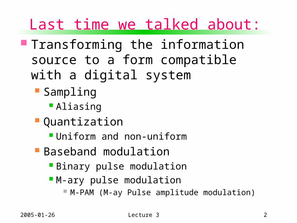
Last time we talked about: Transforming the information source
to a form compatible with a digital system Sampling
Aliasing Quantization
Uniform and non-uniform Baseband modulation
Binary pulse modulation M-ary pulse modulation
M-PAM (M-ay Pulse amplitude modulation)

2005-01-26 Lecture 3 3
Formatting and transmission of baseband signal
Information (data) rate: Symbol rate :
For real time transmission:
Sampling at rate
(sampling time=Ts)
Quantizing each sampled value to one of the L levels in quantizer.
Encoding each q. value to bits
(Data bit duration Tb=Ts/l)
Encode
PulsemodulateSample Quantize
Pulse waveforms(baseband signals)
Bit stream(Data bits)
Format
Digital info.
Textual info.
Analog info.
source
Mapping every data bits to a symbol out of M symbols and transmitting
a baseband waveform with duration T
ss Tf /1 Ll 2log
Mm 2log
[bits/sec] /1 bb TR ec][symbols/s /1 TR
mRRb
2005-01-26 Lecture 3 4
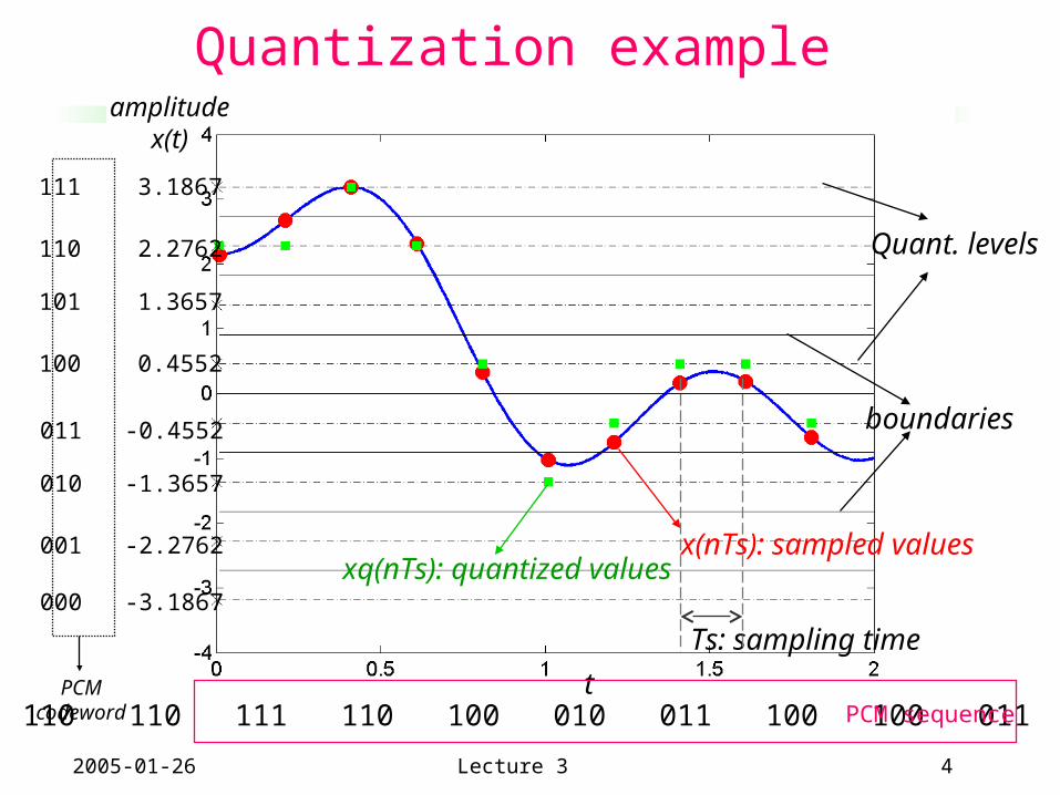
Quantization example
t
Ts: sampling time
x(nTs): sampled valuesxq(nTs): quantized values
boundaries
Quant. levels
111 3.1867
110 2.2762
101 1.3657
100 0.4552
011 -0.4552
010 -1.3657
001 -2.2762
000 -3.1867
PCMcodeword 110 110 111 110 100 010 011 100 100 011 PCM sequence
amplitudex(t)
2005-01-26 Lecture 3 5
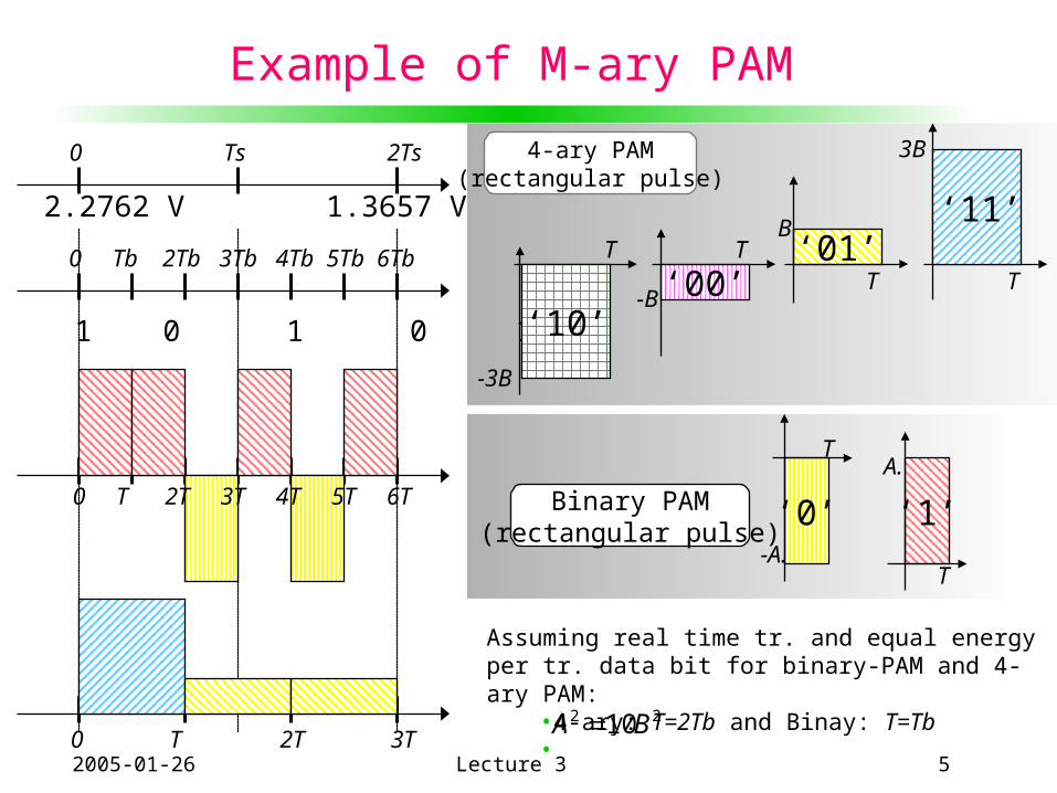
Example of M-ary PAM
0 Tb 2Tb 3Tb 4Tb 5Tb 6Tb
0 Ts 2Ts
0 T 2T 3T
2.2762 V 1.3657 V
1 1 0 1 0 1-B
B
T‘01’
3B
TT
-3B
T
‘00’‘10’
‘1’
A.
T
‘0’
T
-A.
Assuming real time tr. and equal energy per tr. data bit for binary-PAM and 4-ary PAM:
•4-ary: T=2Tb and Binay: T=Tb•
4-ary PAM(rectangular pulse)
Binary PAM(rectangular pulse)
‘11’
0 T 2T 3T 4T 5T 6T
22 10BA
2005-01-26 Lecture 3 6
Today we are going to talk about:
Receiver structure Demodulation (and sampling) Detection
First step for designing the receiver Matched filter receiver
Correlator receiver Vector representation of signals
(signal space), an important tool to facilitate Signals presentations, receiver
structures Detection operations
2005-01-26 Lecture 3 7
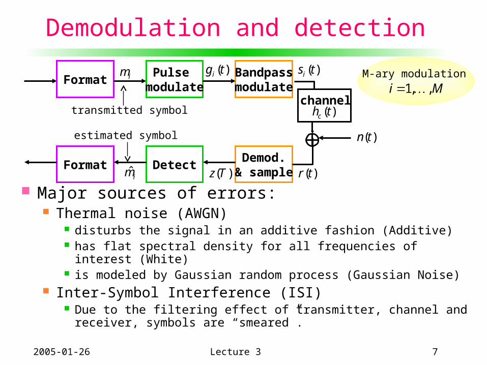
Demodulation and detection
Major sources of errors: Thermal noise (AWGN)
disturbs the signal in an additive fashion (Additive) has flat spectral density for all frequencies of interest
(White) is modeled by Gaussian random process (Gaussian Noise)
Inter-Symbol Interference (ISI) Due to the filtering effect of transmitter, channel and
receiver, symbols are “smeared”.
FormatPulse
modulateBandpassmodulate
Format DetectDemod.
& sample
)(tsi)(tgiim
im̂ )(tr)(Tz
channel)(thc
)(tn
transmitted symbol
estimated symbol
Mi ,,1M-ary modulation
2005-01-26 Lecture 3 8
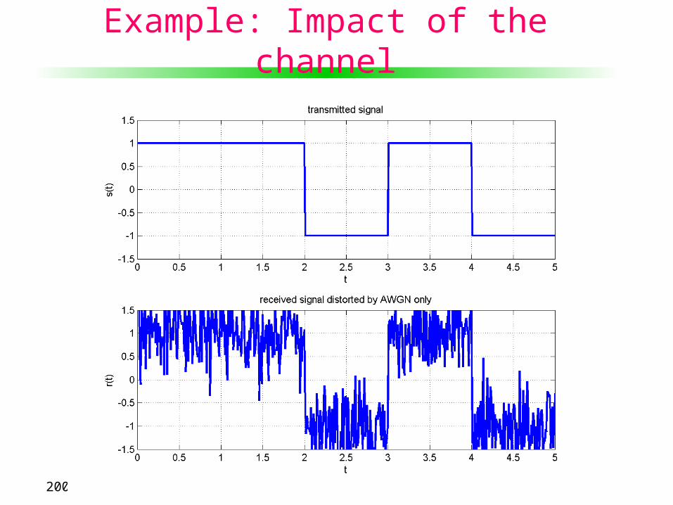
Example: Impact of the channel
2005-01-26 Lecture 3 9
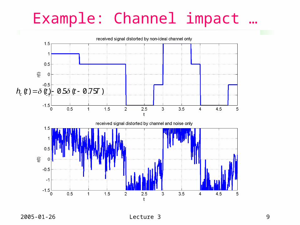
Example: Channel impact …
)75.0(5.0)()( Tttthc
2005-01-26 Lecture 3 10
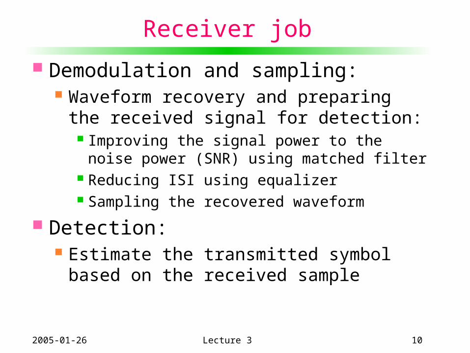
Receiver job
Demodulation and sampling: Waveform recovery and preparing the
received signal for detection: Improving the signal power to the noise
power (SNR) using matched filter Reducing ISI using equalizer Sampling the recovered waveform
Detection: Estimate the transmitted symbol
based on the received sample
2005-01-26 Lecture 3 11
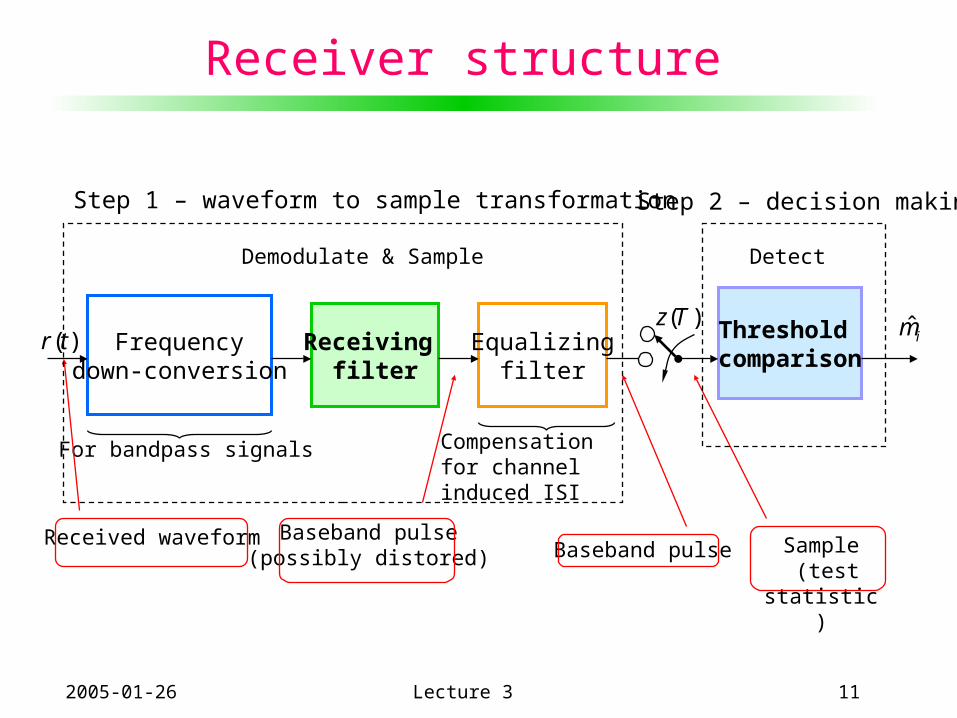
Receiver structure
Frequencydown-conversion
Receiving filter
Equalizingfilter
Threshold comparison
For bandpass signals Compensation for channel induced ISI
Baseband pulse(possibly distored)
Sample (test statistic)
Baseband pulseReceived waveform
Step 1 – waveform to sample transformation Step 2 – decision making
)(tr)(Tz
im̂
Demodulate & Sample Detect
2005-01-26 Lecture 3 12
Baseband and bandpass
Bandpass model of detection process is equivalent to baseband model because: The received bandpass waveform is first
transformed to a baseband waveform. Equivalence theorem:
Performing bandpass linear signal processing followed by heterodying the signal to the baseband, yields the same results as heterodying the bandpass signal to the baseband , followed by a baseband linear signal processing.

2005-01-26 Lecture 3 13
Steps in designing the receiver
Find optimum solution for receiver design with the following goals:
1. Maximize SNR2. Minimize ISI
Steps in design: Model the received signal Find separate solutions for each of the goals.
First, we focus on designing a receiver which maximizes the SNR.
2005-01-26 Lecture 3 14
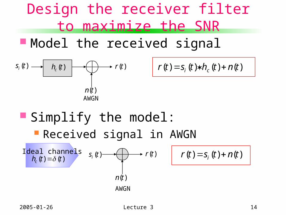
Design the receiver filter to maximize the SNR
Model the received signal
Simplify the model: Received signal in AWGN
)(thc)(tsi
)(tn
)(tr
)(tn
)(tr)(tsiIdeal channels
)()( tthc
AWGN
AWGN
)()()()( tnthtstr ci
)()()( tntstr i

2005-01-26 Lecture 3 15
Matched filter receiver
Problem: Design the receiver filter such that the
SNR is maximized at the sampling time when
is transmitted. Solution:
The optimum filter, is the Matched filter, given by
which is the time-reversed and delayed version of the
conjugate of the transmitted signal
)(th
)()()( * tTsthth iopt )2exp()()()( * fTjfSfHfH iopt
Mitsi ,...,1 ),(
T0 t
)(tsi
T0 t
)()( thth opt
2005-01-26 Lecture 3 16
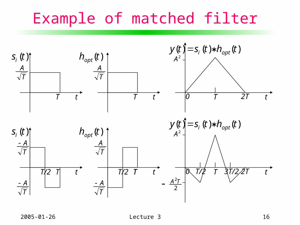
Example of matched filter
T t T t T t0 2T
)()()( thtsty opti 2A)(tsi )(thopt
T t T t T t0 2T
)()()( thtsty opti 2A)(tsi )(thopt
T/2 3T/2T/2 TT/2
2
2TA
TA
TA
TA
TA
TA
TA

2005-01-26 Lecture 3 17
Properties of the matched filter1. The Fourier transform of a matched filter output with the matched
signal as input is, except for a time delay factor, proportional to the ESD of the input signal.
2. The output signal of a matched filter is proportional to a shifted version of the autocorrelation function of the input signal to which the filter is matched.
3. The output SNR of a matched filter depends only on the ratio of the signal energy to the PSD of the white noise at the filter input.
4. Two matching conditions in the matched-filtering operation: spectral phase matching that gives the desired output peak at time T. spectral amplitude matching that gives optimum SNR to the peak
value.
)2exp(|)(|)( 2 fTjfSfZ
sss ERTzTtRtz )0()()()(
2/max
0N
E
N
S s
T
2005-01-26 Lecture 3 18
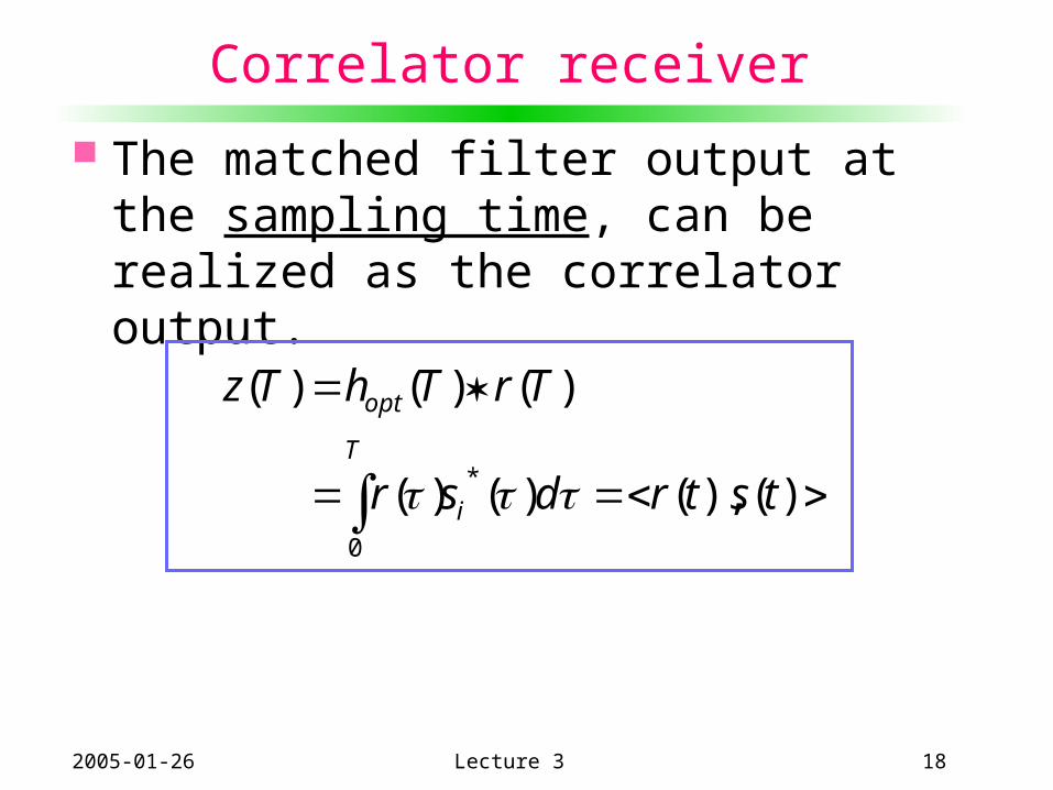
Correlator receiver
The matched filter output at the sampling time, can be realized as the correlator output.
)(),()()(
)()()(
*
0
tstrdsr
TrThTz
i
T
opt
2005-01-26 Lecture 3 19
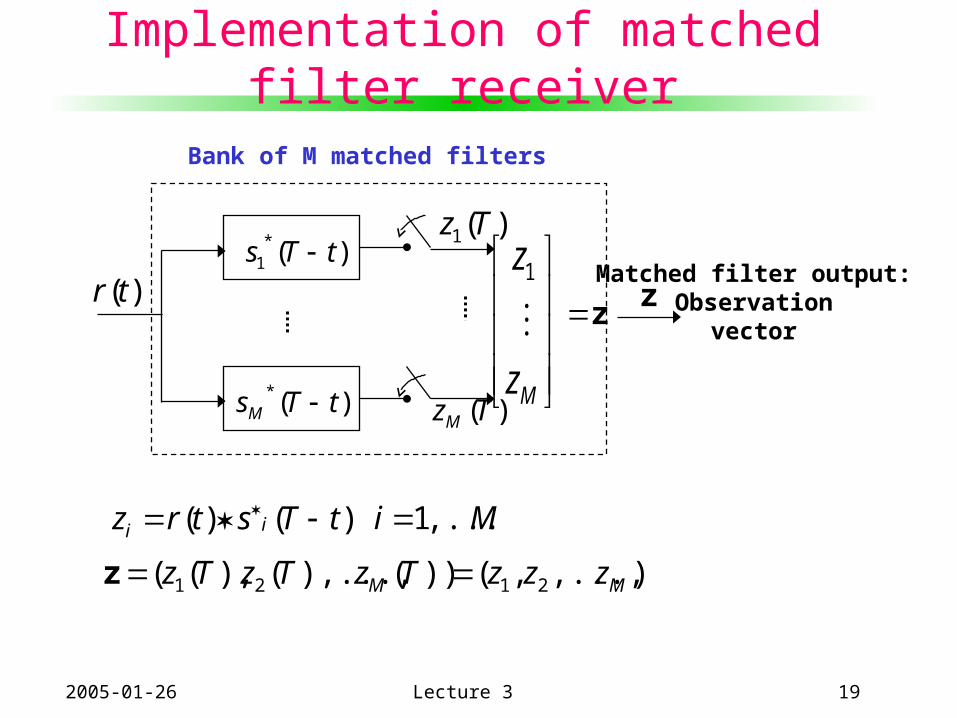
Implementation of matched filter receiver
Mz
z
1
z)(tr
)(1 Tz)(*
1 tTs
)(* tTsM )(TzM
z
Bank of M matched filters
Matched filter output:Observation
vector
)()( tTstrz ii Mi ,...,1
),...,,())(),...,(),(( 2121 MM zzzTzTzTz z
2005-01-26 Lecture 3 20
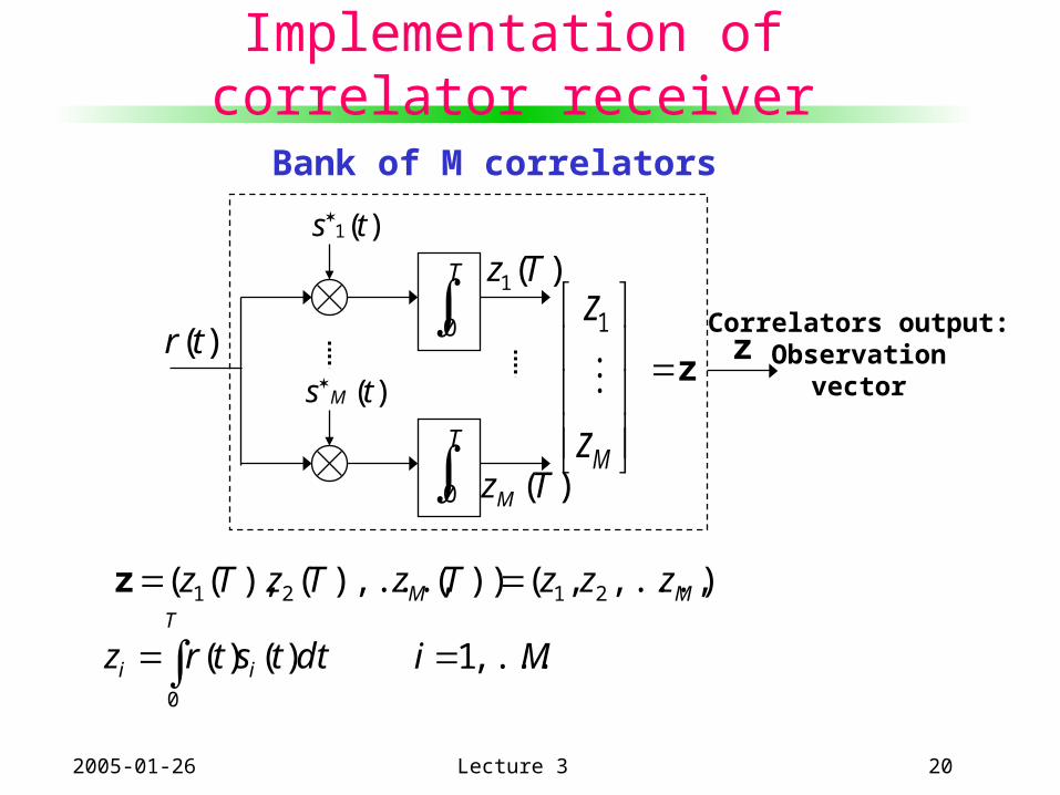
Implementation of correlator receiver
dttstrz i
T
i )()(0
T
0
)(1 ts
T
0
)(ts M
Mz
z
1
z)(tr
)(1 Tz
)(TzM
z
Bank of M correlators
Correlators output:Observation
vector
),...,,())(),...,(),(( 2121 MM zzzTzTzTz z
Mi ,...,1
2005-01-26 Lecture 3 21
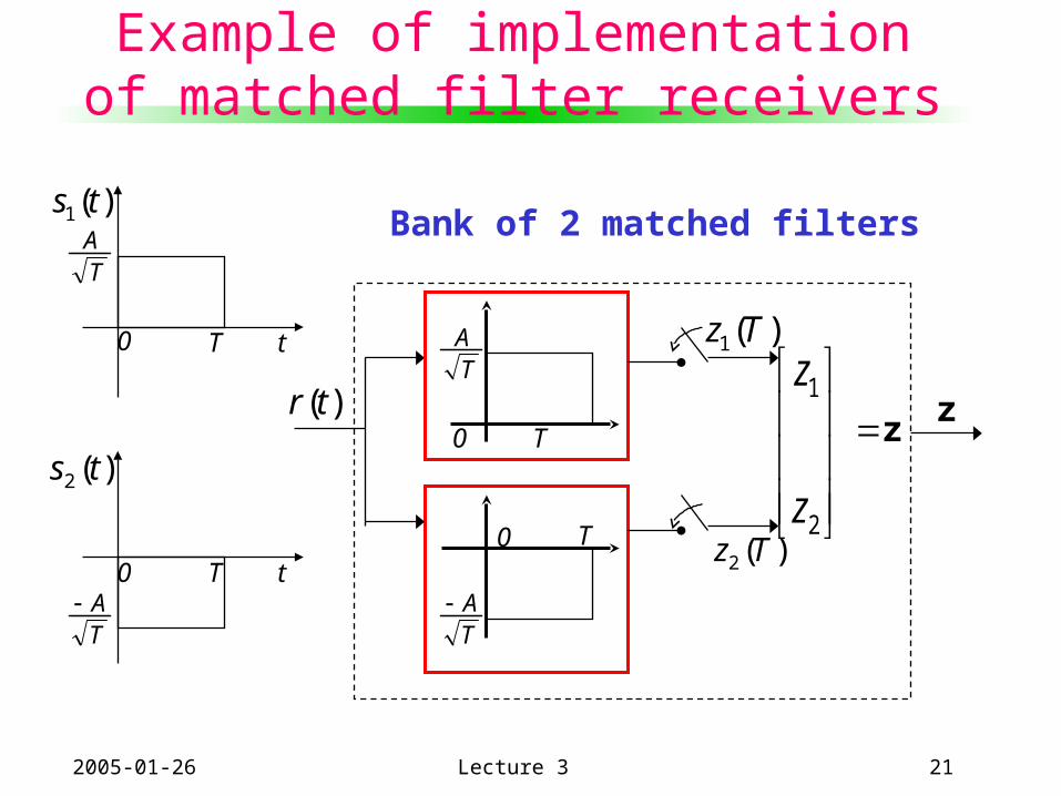
Example of implementation of matched filter receivers
2
1
z
zz
)(tr
)(1 Tz
)(2 Tz
z
Bank of 2 matched filters
T t
)(1 ts
T t
)(2 tsT
T0
0
TA
TA
TA
TA
0
0

2005-01-26 Lecture 3 22
Signal space What is a signal space?
Vector representations of signals in an N-dimensional orthogonal space
Why do we need a signal space? It is a means to convert signals to vectors and
vice versa. It is a means to calculate signals energy and
Euclidean distances between signals. Why are we interested in Euclidean
distances between signals? For detection purposes: The received signal is
transformed to a received vectors. The signal which has the minimum distance to the received signal is estimated as the transmitted signal.

2005-01-26 Lecture 3 23
Schematic example of a signal space
),()()()(
),()()()(
),()()()(
),()()()(
212211
323132321313
222122221212
121112121111
zztztztz
aatatats
aatatats
aatatats
z
s
s
s
)(1 t
)(2 t),( 12111 aas
),( 22212 aas
),( 32313 aas
),( 21 zzz
Transmitted signal alternatives
Received signal at matched filter output
2005-01-26 Lecture 3 24
Signal space
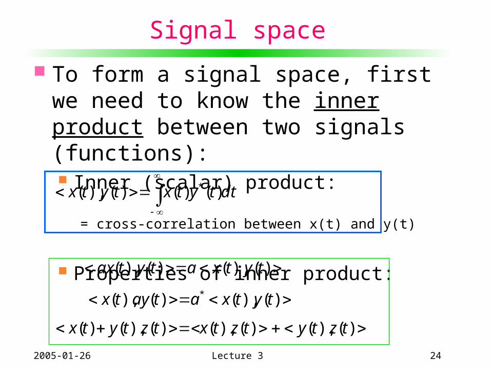
To form a signal space, first we need to know the inner product between two signals (functions): Inner (scalar) product:
Properties of inner product:
dttytxtytx )()()(),( *
= cross-correlation between x(t) and y(t)
)(),()(),( tytxatytax
)(),()(),( * tytxataytx
)(),()(),()(),()( tztytztxtztytx
2005-01-26 Lecture 3 25
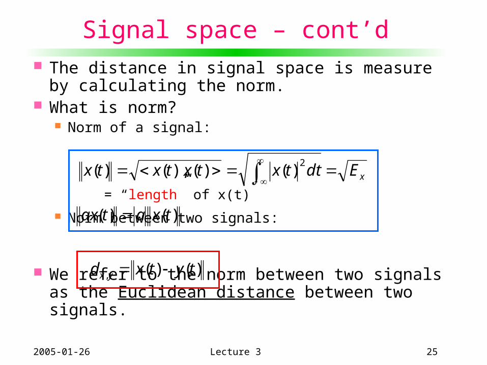
Signal space – cont’d The distance in signal space is measure by
calculating the norm. What is norm?
Norm of a signal:
Norm between two signals:
We refer to the norm between two signals as the Euclidean distance between two signals.
xEdttxtxtxtx
2)()(),()(
)()( txatax
)()(, tytxd yx
= “length” of x(t)
2005-01-26 Lecture 3 26
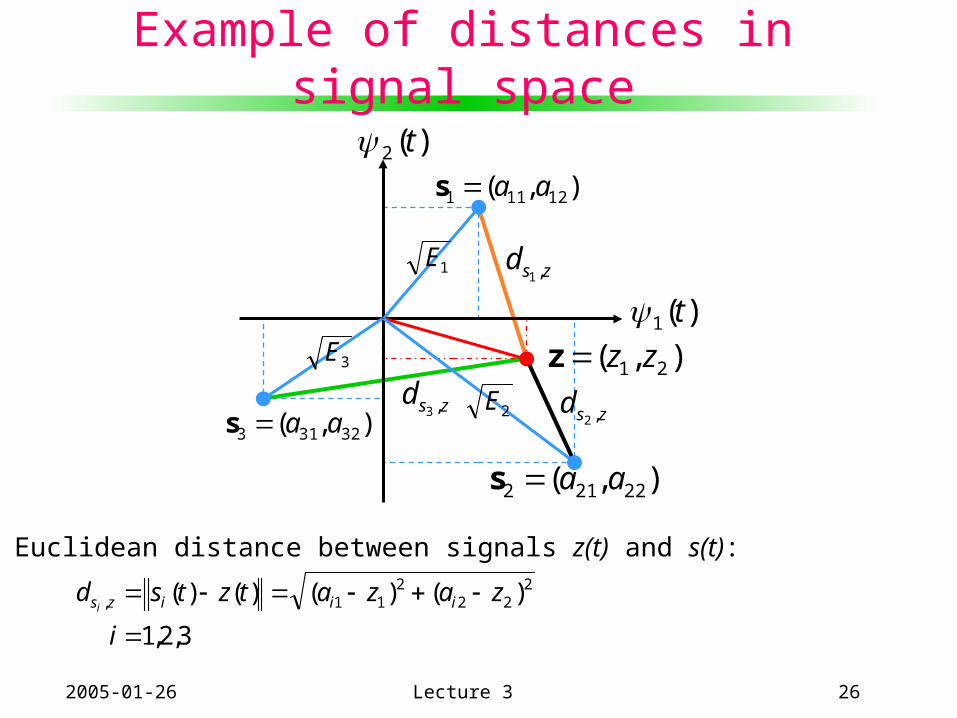
Example of distances in signal space
)(1 t
)(2 t),( 12111 aas
),( 22212 aas
),( 32313 aas
),( 21 zzz
zsd ,1
zsd ,2zsd ,3
The Euclidean distance between signals z(t) and s(t):
3,2,1
)()()()( 222
211,
i
zazatztsd iiizsi
1E
3E
2E
2005-01-26 Lecture 3 27
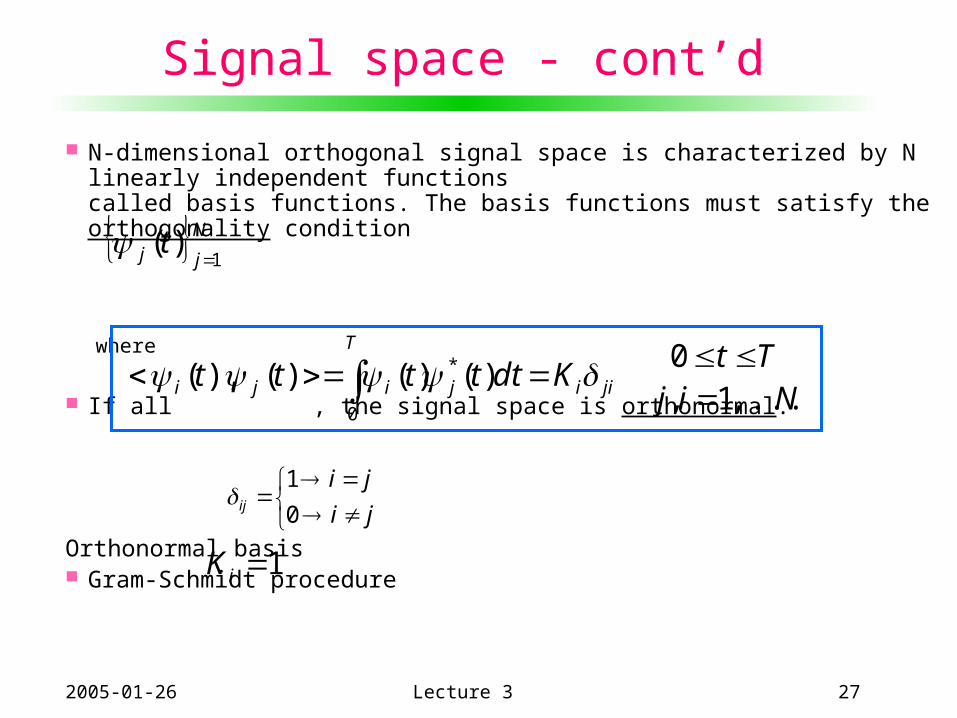
Signal space - cont’d
N-dimensional orthogonal signal space is characterized by N linearly independent functions called basis functions. The basis functions must satisfy the orthogonality condition
where
If all , the signal space is orthonormal.
Orthonormal basis Gram-Schmidt procedure
Njj t
1)(
jiij
T
iji Kdttttt )()()(),( *
0
Tt 0Nij ,...,1,
ji
jiij 0
1
1iK
2005-01-26 Lecture 3 28
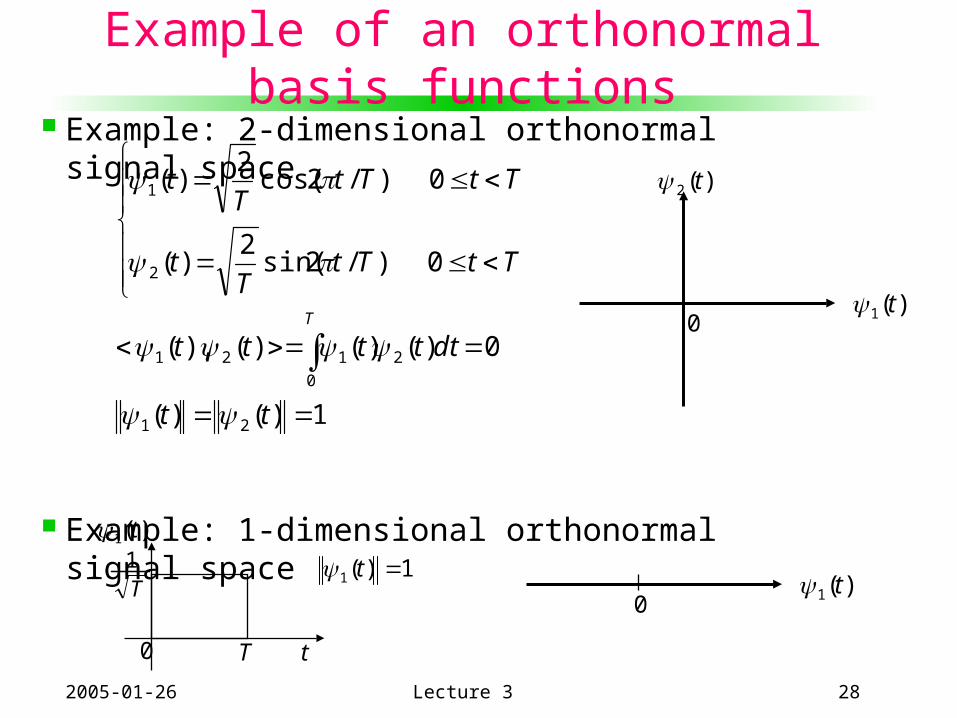
Example of an orthonormal basis functions
Example: 2-dimensional orthonormal signal space
Example: 1-dimensional orthonormal signal space
1)()(
0)()()(),(
0)/2sin(2
)(
0)/2cos(2
)(
21
2
0
121
2
1
tt
dttttt
TtTtT
t
TtTtT
t
T
T t
)(1 t
T1
0
)(1 t
)(2 t
0
1)(1 t)(1 t
0
2005-01-26 Lecture 3 29
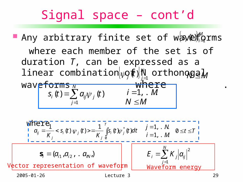
Signal space – cont’d
Any arbitrary finite set of waveforms
where each member of the set is of duration T, can be expressed as a linear combination of N orthonogal waveforms where .
where
Mii ts 1)(
Njj t
1)(
MN
N
jjiji tats
1
)()( Mi ,...,1MN
dtttsK
ttsK
aT
jij
jij
ij )()(1
)(),(1
0
* Tt 0Mi ,...,1Nj ,...,1
),...,,( 21 iNiii aaas2
1ij
N
jji aKE
Vector representation of waveform Waveform energy
2005-01-26 Lecture 3 30
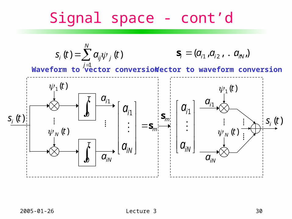
Signal space - cont’d
N
jjiji tats
1
)()( ),...,,( 21 iNiii aaas
iN
i
a
a
1
)(1 t
)(tN
1ia
iNa
)(tsi
T
0
)(1 t
T
0
)(tN
iN
i
a
a
1
ms)(tsi
1ia
iNa
ms
Waveform to vector conversion Vector to waveform conversion
2005-01-26 Lecture 3 31
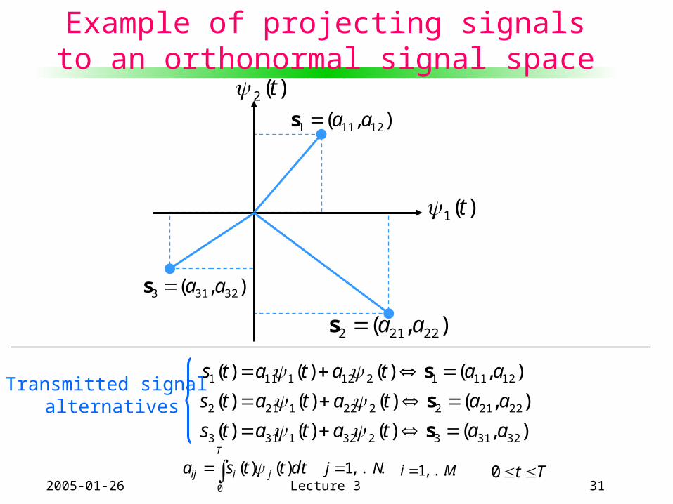
Example of projecting signals to an orthonormal signal space
),()()()(
),()()()(
),()()()(
323132321313
222122221212
121112121111
aatatats
aatatats
aatatats
s
s
s
)(1 t
)(2 t),( 12111 aas
),( 22212 aas
),( 32313 aas
Transmitted signal alternatives
dtttsaT
jiij )()(0 Tt 0Mi ,...,1Nj ,...,1
2005-01-26 Lecture 3 32
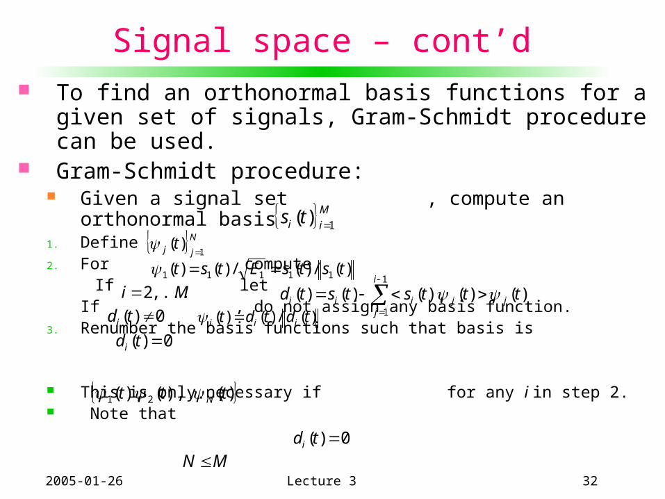
Signal space – cont’d To find an orthonormal basis functions for a given
set of signals, Gram-Schmidt procedure can be used.
Gram-Schmidt procedure: Given a signal set , compute an orthonormal
basis1. Define2. For compute If let
If , do not assign any basis function.3. Renumber the basis functions such that basis is
This is only necessary if for any i in step 2. Note that
Mii ts 1)(
Njj t
1)(
)(/)(/)()( 11111 tstsEtst Mi ,...,2
1
1
)()(),()()(i
jjjiii tttststd
0)( tdi )(/)()( tdtdt iii 0)( tdi
)(),...,(),( 21 ttt N
0)( tdi
MN
2005-01-26 Lecture 3 33
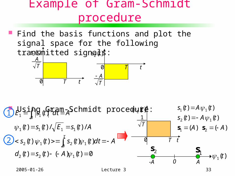
Example of Gram-Schmidt procedure
Find the basis functions and plot the signal space for the following transmitted signals:
Using Gram-Schmidt procedure:
T t
)(1 ts
T t
)(2 ts
)( )(
)()(
)()(
21
12
11
AA
tAts
tAts
ss
)(1 t-A A0
1s2s
TA
TA
0
0
T t
)(1 t
T1
0
0)()()()(
)()()(),(
/)(/)()(
)(
122
0 1212
1111
0
22
11
tAtstd
Adtttstts
AtsEtst
AdttsE
T
T
1
2
2005-01-26 Lecture 3 34
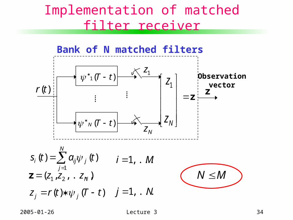
Implementation of matched filter receiver
)(tr
1z)(1 tT
)( tTN Nz
Bank of N matched filters
Observationvector
)()( tTtrz jj Nj ,...,1
),...,,( 21 Nzzzz
N
jjiji tats
1
)()(
MN Mi ,...,1
Nz
z1
z z
2005-01-26 Lecture 3 35
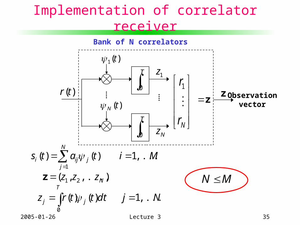
Implementation of correlator receiver
),...,,( 21 Nzzzz
Nj ,...,1dtttrz j
T
j )()(0
T
0
)(1 t
T
0
)(tN
Nr
r
1
z)(tr
1z
Nz
z
Bank of N correlators
Observationvector
N
jjiji tats
1
)()( Mi ,...,1
MN
2005-01-26 Lecture 3 36
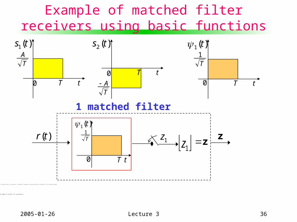
Example of matched filter receivers using basic functions
Number of matched filters (or correlators) is reduced by 1 compared to using matched filters (correlators) to the transmitted signal.
Reduced number of filters (or correlators)
T t
)(1 ts
T t
)(2 ts
T t
)(1 t
T1
0
1z z)(tr z
1 matched filter
T t
)(1 t
T1
0
1z
TA
TA0
0
2005-01-26 Lecture 3 37
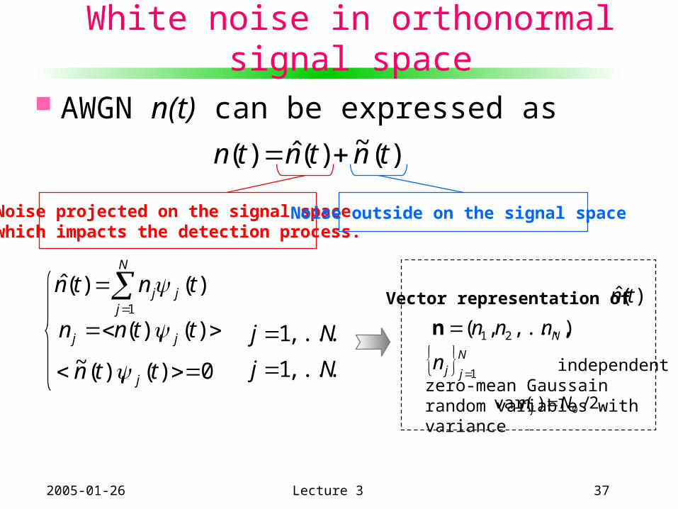
White noise in orthonormal signal space
AWGN n(t) can be expressed as
)(~)(ˆ)( tntntn
Noise projected on the signal space which impacts the detection process.
Noise outside on the signal space
)(),( ttnn jj
0)(),(~ ttn j
)()(ˆ1
tntnN
jjj
Nj ,...,1
Nj ,...,1
Vector representation of
),...,,( 21 Nnnnn
)(ˆ tn
independent zero-mean Gaussain random variables with variance
Njjn
1
2/)var( 0Nn j