modulation of internal gravity waves ina multi-scale
TRANSCRIPT
Generated using version 3.0 of the official AMS LATEX template
Modulation of Internal Gravity Waves in a Multi-scale Model for
Deep Convection on Mesoscales
Daniel Ruprecht ∗ and Rupert Klein
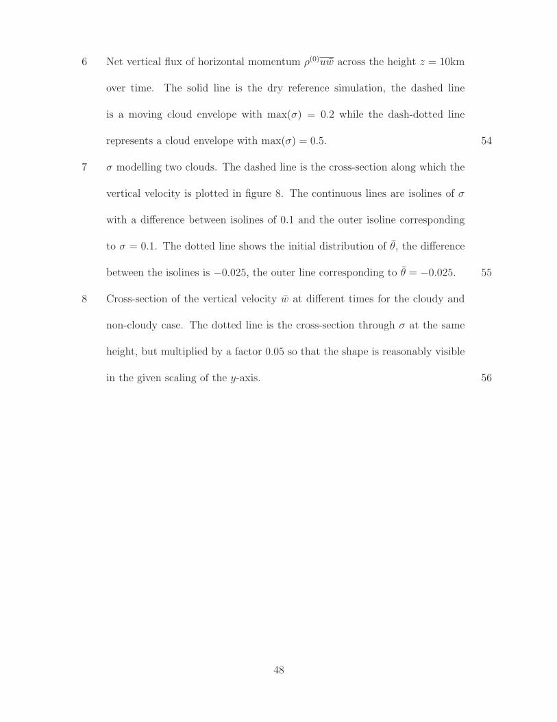
FB Mathematik, Freie Universitat Berlin, Germany
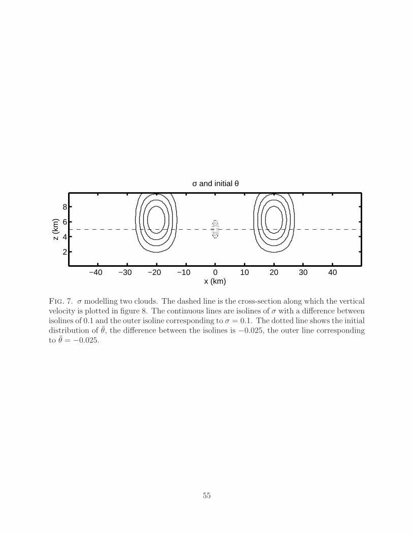
Andrew J. Majda
Courant Institute of Mathematical Sciences, New York University
∗Corresponding author address: Daniel Ruprecht, FB Mathematik, Freie Universitat Berlin, Arnimallee
6, 14195 Berlin , Germany.
E-mail: [email protected]
1

ABSTRACT
Starting from the conservation laws for mass, momentum, and energy together with a three
species, bulk micro-physics model, a model for the interaction of internal gravity waves and
deep convective hot towers is derived using multi-scale asymptotic techniques. From the
leading order equations, a closed model for the large-scale flow is obtained analytically by
applying horizontal averages conditioned on the small-scale hot towers. No closure approx-
imations are required besides adopting the asymptotic limit regime which the analysis is
based on. The resulting model is an extension of the anelastic equations linearized about
a constant background flow. Moist processes enter through the area fraction of saturated
regions and through two additional dynamic equations describing the coupled evolution of
the conditionally averaged small-scale vertical velocity and buoyancy. A two-way coupling
between the large-scale dynamics and these small-scale quantities is obtained: moisture re-
duces the effective stability for the large-scale flow, and micro-scale up- and downdrafts
define a large-scale averaged potential temperature source term. In turn, large-scale vertical
velocities induce small-scale potential temperature fluctuations due to the discrepancy in
effective stability between saturated and non-saturated regions.
The dispersion relation and group velocity of the system are analyzed and moisture is
found to have several effects: it (i) reduces vertical energy transport by waves, (ii) increases
vertical wavenumbers but decreases the slope at which wave packets travel, (iii) introduces
a new lower horizontal cut-off wavenumber besides the well-known high wavenumber cut-off,
and (iv) moisture can cause critical layers. Numerical examples reveal the effects of moisture
on steady-state and time-dependent mountain waves in the present hot-tower regime.
1
1. Introduction
Internal gravity waves are one prominent feature of atmospheric flows on lengthscales
from approx. 10 to 100 km and are responsible for a number of important effects. As
Bretherton and Smolarkiewicz (1989) and Lane and Reeder (2001) show, convecting clouds
emit gravity waves which alter their environment, rendering it favorable for further convec-
tion by reducing convective inhibition (CIN). Chimonas et al. (1980) investigate a feedback
mechanism between saturated regions and gravity waves that can trigger convection. They
hypothesize that gravity waves contribute to the organization of individual convective events
into larger scale structures like squall lines. Vertically propagating gravity waves are asso-
ciated with vertical transport of horizontal momentum. The dissipation of these waves in
the stratosphere exerts a net force on middle atmospheric flows known as “gravity-wave
drag” (GWD), see, e.g., Sawyer (1959); Lindzen (1981). McLandress (1998) demonstrates
the necessity of including the effects of GWD in “global circulation models” (GCM) to ob-
tain realistic flows. Joos et al. (2008) find that gravity waves are also important for the
parameterization of cirrus clouds. Because GCMs have a spatial resolution of 100− 200 km,
gravity waves cannot be resolved in these models and their effects have to be parameterized.
Kim et al. (2003) provide an overview of concepts of GWD parameterizations in GCMs.
Moisture in the atmosphere significantly affects the propagation of internal waves. Bar-
cilon et al. (1979) propose a model for steady, hydrostatic flow over a mountain with re-
versible moist dynamics. This model distinguishes between saturated and non-saturated
regions by a switching function that depends on the vertical displacement of a parcel: if
the parcel is displaced beyond the lifting condensation level, it is treated as saturated and
2
the dry stability frequency is replaced by the reduced moist stability frequency. Barcilon
et al. (1980) extend the model to non-hydrostatic flows with irreversible condensation, and
Barcilon and Fitzjarrald (1985) to nonlinear, steady flow. These authors find that moisture
can significantly reduce the mountain drag which is closely related to the wave drag. Jusem
and Barcilon (1985) employ a nonlinear, non-steady, non-hydrostatic anelastic model that
explicitly includes the mixing ratios of liquid water and vapor to define heating source terms
for the potential temperature. Besides finding again that moisture can reduce drag, they
also find that moisture does reduce the wave intensity and increases the vertical wavelength.
While the first result is also found in the present paper, instead of an increased vertical
wavelength, we observe an increase of the vertical wavenumber by moisture, corresponding
to a reduced vertical wavelength.
Durran and Klemp (1983) employ a fully compressible model combined with prognostic
equations for water vapor, rain water, and cloud water to simulate moist mountain waves.
They also find that moisture reduces the vertical flux of momentum and the amplitude of the
generated wave patterns. Further, they observe an increase in vertical wavelength for nearly
hydrostatic waves. Attenuation of gravity waves by moisture and an increase of vertical
wavelength is also found in the analysis of wave propagation in a fully saturated atmosphere
in Einaudi and Lalas (1973).
Although there is extensive literature dealing with the parameterization of drag from
convectively generated waves, there are very few attempts to include the effect of moisture
in parameterizations of orographic waves. In their review, Kim et al. (2003) mention only
the work of Surgi (1989), investigating the introduction of a stability frequency modified by
moisture into the orographic GWD parameterization.
3
Klein and Majda (2006) derive a multi-scale model for the interaction of non-hydrostatic
internal gravity waves with moist deep convective towers from the conservation laws of mass,
momentum, and energy combined with a classical bulk micro-physics scheme. In agreement
with the regime of non-rotating, non-hydrostatic gravity waves described by Gill (1982),
Ch. 8, the characteristic horizontal and vertical scales for the gravity waves are assumed
comparable to the pressure scale height, hsc ∼ 10 km. LeMone and Zipser (1980) provide
an indication for the characteristic horizontal scales of the narrow deep convective towers:
they analyze data obtained during the GATE experiment and find that the median diameter
of “convective events” related to tropical cumulonimbus clouds is about 900 m, see also
Stevens (2005). Thus a horizontal “micro”-scale of 1 km is used as the second horizontal
lengthscale in the multi-scale ansatz to describe the tower-scale dynamics. The assumed
timescale of 100 s is compatible with the typical value of 0.01 s−1 for the stability frequency
in the troposphere.
By using an asymptotic ansatz representing these scales, this paper presents the deriva-
tion of a reduced model for modulation of internal waves by moisture. For a first reading,
one can study the summary of the model in 1a, skip the technical derivation in 2 and go
immediately to the new phenomena and application of the model in sections 3 and 4. The
reduced model allows for an analytical investigation, concisely revealing a number of mecha-
nisms by which moisture does affect internal waves. It confirms already known facts but also
allows to hypothesize new effects that might be important for improved parameterizations
of internal waves. Further, the model equations themselves might serve as a starting point
for the development of such parameterizations.
The used asymptotic ansatz is the one introduced by Klein and Majda (2006) with
4
the slight modification of adding a constant, horizontal background flow. Using weighted
averages, the obtained leading order multi-scale equations are converted into a closed system
of equations for the gravity wave scale only. In this system, the effective vertical mass fluxes
are obtained analytically so that no additional physical closure assumptions beyond those
made in adopting the asymptotic scaling regime are required. The resulting equations are
an extension of the anelastic equations, linearized around a moist adiabatic, constant wind
background flow. Mathematical analysis of these equations reveals, among other effects,
that moisture introduces a lower horizontal cut-off wavenumber, the existence of which is,
to the authors’ knowledge, a new hypothesis. The essential moisture-related parameter
in the model is the area fraction of saturated regions on the micro-scale, reminiscent of a
smaller scale version of the “cloud cover fraction”, a parameter routinely computed and
used in GCMs. Jakob and Klein (1999) discuss this parameter in the context of micro-
physical parameterizations in the ECMWF1 model. They find that a uniform value for
cloud cover over one cell is not sufficient and divide the cell into a number of sub-columns so
as to approximately represent a spatially inhomogeneous distribution of cloud cover inside
a cell. Trying to link the saturated area fraction arising in the present model to such
decompositions of cloud cover might be a promising ansatz to include moisture effects in
GWD parameterizations in a systematic way.
1European Centre for Medium-Range Weather Forecast
5
a. Summary of the model
The new model for gravity wave–convective tower interactions consists of equations de-
scribing linearized, anelastic moist dynamics plus two equations for the conditionally aver-
aged tower-scale dynamics. u is the horizontal velocity, w the averaged vertical velocity and
θ the average potential temperature. w′ and θ′ are conditional averages of deviations from w
and θ within the deep convective clouds. Here π is the Exner function, ρ(0) the leading order
background density and θ(2)z the background stratification while u∞ is a constant, horizontal
background velocity. The source term C− is a constant cooling term related to evaporating
rain in non-saturated areas, and σ is the saturated area fraction mentioned earlier. See
section 2 for details.
Linearized, anelastic moist dynamics:
uτ + u∞ux + πx = 0
wτ + u∞wx + πz = θ
θτ + u∞θx + (1− σ) θ(2)z w = θ(2)z w′ + C−
(ρ0u)x + (ρ0w)z = 0
(1)
Averaged tower-scale dynamics:
w′τ + u∞w′
x = θ′
θ′τ + u∞θ′x + σθ(2)z w′ = σ (1− σ) θ(2)z w − σC−.(2)
Moisture affects the large-scale dynamics given by (1) in two ways. It reduces the effective
stability of the atmosphere by a factor of 1− σ, representing the effect that if a parcel rises
and starts condensating water, the release of latent heat will effectively reduce the restoring
6
force the parcel experiences. Because of the short timescale in this model, the only conversion
mechanism between moist quantities that has a leading order effect is evaporation of cloud
water into vapor and condensation of vapor into cloud water in fully saturated regions. As
a consequence, σ itself does not change with time in the present model except for being
advected by the mean flow. In fact, for the scalings assumed in the present derivation,
the physical effect of non-saturated rising parcels eventually becoming saturated when lifted
sufficiently is not present. An extension of the model to capture this effect is the subject of
current work and beyond the scope of the present paper. See also our comments in section
3e.
The release and consumption of latent heat by averaged small-scale up- and downdrafts
in saturated areas is described by the source term θ(2)z w′ in (1)3. A positive w′ results in a
positive contribution to θ, modelling latent heat release whereas a negative w′ models latent
heat consumption. Yet, the micro-scale model not only provides the source term for the
large-scale dynamics but is also affected by them in return through the w source term on the
right hand side of (2)2. Finally, for the chosen time and lengthscales, the mass conservation
equation reduces to the anelastic divergence constraint (1)4.
Note that if all moisture related terms vanish, i.e., for σ = 0, C− = 0 and w′(τ = 0) =
θ′(τ = 0) = 0, the system in (1) reduces to the anelastic equations linearized around a
constant-wind background flow with stable stratification, θ(2)z > 0, see, e.g., Davies et al.
(2003),
7

uτ + u∞ux + πx = 0
wτ + u∞wx + πz = θ
θτ + u∞θx + θ(2)z w = 0
(ρ0u)x + (ρ0w)z = 0.
(3)
2. Derivation of the model
This section provides the derivation of the model from eqs. (1), (2). The present modifi-
cation of the original asymptotic regime considered by Klein and Majda (2006) is developed
in section 2a together with a justification for the particular scaling of the constant horizontal
background wind velocity. Section 2b describes the closure of the leading order equations
by weighted averages.
a. Multiple scales ansatz
In the derivation by Klein and Majda (2006), three primary dimensionless parameters
occur: the Mach-number M, describing the ratio of a typical flow velocity uref to the speed of
sound waves, the barotropic Froude number Fr, describing the ratio of a typical flow velocity
to the speed of external gravity waves and the bulk micro-scale Rossby radius RoB, providing
a measure of the importance of rotational effects for flows on the bulk micro-scale. These
parameters are defined as
M =uref
√
pref/ρref, Fr =
uref√ghsc
, RoB =uref
lbulkΩ(4)
8
where hsc is the pressure scale height, lbulk is the lengthscale of the bulk micro-physics, pref
and ρref are typical values for pressure and density, Ω is the rate of earth’s rotation and g
the gravity acceleration. Following Majda and Klein (2003), these parameters are related to
a universal expansion parameter ε in the following distinguished limit
M ∼ Fr ∼ ε2, RoB ∼ ε−1 as ε → 0. (5)
The scaling of a fourth dimensionless parameter, the baroclinic Froude number, will be
discussed shortly in the context of eq. (10).
The starting point of the model development are the conservation laws for mass, momen-
tum, and energy combined with a slightly modified version of the bulk micro-physics model
from Grabowski (1998). The prognostic quantities in the original equations are the horizon-
tal velocity u, vertical velocity w, density ρ, pressure p, potential temperature θ, and the
mixing ratios of water vapor qv, cloud water qc, and rain water qr. The scales considered in
the derivation are a timescale of tτ ≈ 100s, a vertical lengthscale equal to the pressure scale
height hsc ≈ 10km and two horizontal scales l ≈ 10km and lbulk ≈ 1000m. As discussed in
the introduction, these scales correspond to a combination of the regimes of non-hydrostatic
gravity waves and deep convective towers. To resolve them, new coordinates are introduced
by rescaling the “universal” coordinates x and t, which resolve the reference lengthscale of
lref ≈ 10 km and timescale of tref ≈ 1000 s, by powers of ε. The new coordinates resolving
the short scales are
τ =t
ε, η =
x
ε. (6)
The model distinguishes between saturated and non-saturated regions by a switching func-
9

tion Hqv , defined as
Hqv(qv) =
1 : q(0)v ≥ q
(0)vs (saturated at leading order)
0 : q(0)v < q
(0)vs (non-saturated at leading order)
, (7)
where q(0)v is the leading order water vapor mixing ratio and q
(0)vs is the leading order saturation
water vapor mixing ratio, computed from Bolton’s formula for the saturation vapor pressure.
See Emanuel (1994) for the original formula and Klein and Majda (2006) for the derivation
of an asymptotic expression for qvs. For the warm micro-physics considered here saturated
regions and clouds coincide and Hqv is the leading-order characteristic function for cloudy
patches of air which equals unity inside clouds and zero between them.
We modify the ansatz for the horizontal velocity by introducing a constant background
velocity u∞. To avoid inconsistencies in the derivation, we also add a second coordinate τ ′
corresponding to the timescale set by advection of flows with u∞-velocity over the short,
tower-scale distances resolved by the η coordinate. The terms related to τ ′ will eventually
drop out by sublinear growth conditions and do not appear in the final model. In terms of
ε the new coordinate is
τ ′ =t
ε2. (8)
All quantities depending on η also depend on τ ′. The horizontal velocity is assumed to be
independent of the small horizontal coordinate η, so we use an ansatz
u(x, z, t; ε) = ε−1u∞ + u(0)(x, z, τ) +O(ε). (9)
Although this scaling would formally suggest dimensional values for u∞ of about 100 m s−1, a
value of u∞ = 0.1 corresponding to 10 m s−1, will be used throughout this paper. The reason
for this apparent inconsistency between the asymptotic scaling of u∞ and the actual value
10

used for it is the following: as shown by Klein (2009), the inverse timescales of advection
and internal waves for flows on a lengthscale hsc with a typical velocity of u/uref = O(1) and
a background stratification θ, using the distinguished limit (5), are
dimensional non-dimensional
advection t−1ref : uref
hsc1
internal waves t−1τ : N 1
ε2
√
hsc
θdθdz.
(10)
Thus, except for very weak stratifications of order O(ε4), the advection timescale and the
timescale of internal waves are asymptotically separated in the limit ε → 0. To retain
both effects, i.e., advection and internal gravity waves, in the leading order equations for
a stratification of order O(ε2) as will be used here according to (15), the inverse advection
timescale has to be of order ε−1. For the O(ε−1) scaling of u∞ in (9), (10)1 becomes t−1ref ∼
ε−1uref/hsc ∼ ε−1 as required, and both timescales are of the same order.
One can also see that if the employed timescale is tτ , a O(ε−1) scaling of u is necessary to
address the non-hydrostatic regime by analyzing the scaling of the baroclinic Froude number
(11). It denotes the ratio between advection and wave speed and indicates the importance of
non-hydrostatic effects. For a stratification of order O(ε2), t−1τ ∼ ε−1 while tref ∼ 1 according
to (10). Thus the scaling of Frbaroclinic reads
Frbaroclinic =u
Nlref∼ u
t−1τ hsc
∼ εu
t−1refhsc
= O(
εu
uref
)
(11)
If u∞ = 0, then u/uref = O(1) and Frbaroclinic is of order O(ε), so that non-hydrostatic effects
would not be contained in the leading order equations.
The scale separation revealed in (10) between internal waves for stratifications of order
O(ε2) and advection based on the reference velocity uref in the limit ε → 0 is, however, ob-
11
scured for finite values of ε ≈ 0.1, which are typical for realistic atmospheric flows: let k and
m denote the horizontal and vertical wavenumber of an internal wave. For non-hydrostatic
waves, these are of comparable magnitude. The lengthscale hsc provides a reference value
for both wavenumbers of
kref =2π
hsc
= 2π · 10−4 m−1 . (12)
Now, according to the dispersion relation for internal waves, see e.g., Buhler (2009), the
horizontal phase velocity is
cphase =N√
k2 +m2. (13)
Using a typical value for the stability frequency of N = 0.01 s−1, we obtain a dimensional
value for the phase velocity of
cphase,dim ≈ 10−2 s−1
√2 · 2π · 10−4 m−1
≈ 11m
s. (14)
Thus, while a scaling of u∞ of order O(ε−1) is required to retain advection in the limit ε → 0,
a value of u∞ = 0.1, corresponding to dimensional values of about 10 m s−1, agrees very well
with the timescale of internal waves actually obtained with realistic values of εactual = 0.1.
The reason is that the factor(√
2 · 2π)−1
in (14) is of order O(1) in the limit ε → 0 but is
comparable to εactual = 0.1.
For a reference velocity u∗ref = hscN = 100 m s−1, no separation of the internal wave
time-scale and the advection time-scale occurs. In principle, an equivalent derivation can be
conducted, if the governing equations are non-dimensionalized using u∗ref . This changes the
distinguished limit (5) and the expansions of the horizontal and vertical velocity, avoiding
a ε−1 scaling of the leading order u∞. The small parameter then is the amplitude of wave-
induced perturbations of the velocity field. The justification for setting u∞ = 0.1 is required
12

in this derivation, too.
The potential temperature is expanded about a background stratification θ(z) = 1 +
ǫ2θ(2)(z) as
θ(x, z, t; ǫ) = 1 + ǫ2θ(2)(z) + ǫ3θ(3)(η, x, z, τ, τ ′) +O(ǫ4). (15)
As discussed in Klein and Majda (2006), considering realistic values of convectively available
potential energy (CAPE) constrains deviations of θ from a moist adiabat, showing that θ(2)
should satisfy the moist adiabatic equation
θ(2)z = −Γ∗∗L∗∗q∗∗vsp(0)
q(0)vs,z =: −Lq(0)vs,z . (16)
Expansions about a moist adiabatic background are also considered, for example, in Lipps
and Hemler (1982). In (16) p(0) is the leading order of the pressure and Γ∗∗, L∗∗ and q∗∗vs are
O(1) scaling factors arising from the non-dimensionalization in Klein and Majda (2006).
The expansions of all other dependent variables are adopted from Klein and Majda
(2006), except that variables depending on η in their derivation now also depend on τ ′.
All quantities φ ∈ u, w, θ, π, qv, qc, qr are split below as
φ = φ+ φ (17)
where
φ = limη0→∞
1
2η0
∫ η0
−η0
φ(η)dη (18)
denotes the small-scale average with respect to the η-coordinate, while φ denotes deviations
from this average.
The description of the scalings and the ansatz are basically a repetition of what is done
in Klein and Majda (2006), so the reader is referred to the original work for a detailed
13
discussion. The focus here is the derivation of a closed model from the resulting leading
order equations and an analysis of the model’s properties. The derivation is presented in a
x-z-plane here. This simplifies the notation and numerical examples presented below will be
of this type, too. However, this is not an essential restriction.
The leading order equations for the averages resulting from this ansatz are
u(0)τ + u∞u(0)
x + π(3)x = 0
w(0)τ + u∞w(0)
x + π(3)z = θ(3)
θ(3)τ + u∞θ(3)x + w(0)θ(2)z = L(
HqvC(0)d + (Hqv − 1)C
(0)ev
)
(
ρ(0)u)
x+(
ρ(0)w)
z= 0
(19)
with π(3) = p(3)/ρ(0) and θ(2)z (z) the potential temperature gradient of the background,
C(0)d the leading order source term from vapor condensating to cloud water or cloud water
evaporating, and C(0)ev the leading order source term representing cooling by evaporation of
rain in non-saturated regions. The equations for the perturbations read
w(0)τ + u∞w(0)
x + u(0)wη = θ(3)
θ(3)τ + u∞θ(3)x + u(0)θ(3)η + w(0)θ(2)z =
L(
HqvC(0)d −HqvC
(0)d + (Hqv − 1)C(0)
ev − (Hqv − 1)C(0)ev
)
.
(20)
The leading order equations for the moist species are split into separate equations for the
saturated (Hqv = 1) and the non-saturated (Hqv = 0) cases
14

(i) Saturated
−(
w(0) + w(0))
q(0)vs,z = C(0)d
q(0)r,τ + u∞q(0)r,x + u(0)q(0)r,η = 0
(21)
(ii) Non-Saturated
C∗∗ev
(
q(0)vs − q(0)v
)
√
q(0)r = C(0)
ev
q(0)v,τ + u∞q(0)v,x + u(0)q(0)v,η = 0
q(0)r,τ + u∞q(0)r,x + u(0)q(0)r,η = 0
(22)
C∗∗ev is again a O(1) scaling factor from the non-dimensionalization. q
(0)vs , q
(0)v , q
(0)c and q
(0)r
are the leading order mixing ratios of the saturation water vapor, water vapor, cloud water
and rain water. Key-steps of the derivation can be found in the appendix.
b. Computing the mass flux closure
To obtain a closed set of equations, an equation for HqvC(0)d in (19) will be derived from
the perturbation equations (20) and the leading order equations (21) and (22) obtained from
the bulk micro-scale model. We stress that the closure is computed analytically and does
not require the introduction of additional physical closure assumptions.
Multiply (21)1 by Hqv and average over η to get
−Hqvw(0)q(0)vs,z −Hqvw
(0)q(0)vs,z = HqvC(0)d . (23)
15

Considering (22) and noting that in saturated regions q(0)v = q
(0)vs (z) trivially satisfies the
same transport equation, we find
q(0)v (x, z, η, τ) = q(0)v (x− u∞τ, z, η −∫ τ
0
u(0)(x, z, t′)dt′, 0). (24)
Define
σ(x, z, τ) := Hqv(x, z, η, τ). (25)
As∫ τ
0u(0)(x, z, t′)dt′ is independent of η, we get
σ(x, z, τ) = Hqv(x, z, η, τ)
= Hqv(x− u∞τ, z, η −∫ τ
0
u(0)(x, z, t′)dt′, 0)
= σ(x− u∞τ, z, 0).
(26)
It will turn out that the dynamics induced by moisture in this model can all be tied to this
variable σ. Considering the definition (7) of the switching function Hqv , we see that
σ(x, z, τ) = limη0→∞
1
2η0
∫ η0
−η0
Hqv(x, z, η′, τ)dη′
= limη0→∞
|η ∈ (−η0, η0) : qv(x, z, η, τ) ≥ qvs(z)||(−η0, η0)|
.(27)
So for a fixed point (x, z, τ), σ is the area fraction of saturated regions on the η-scale. Using
(25) and (16) we can write (23) as
L−1σw(0)θ(2)z + L−1Hqvw(0)θ(2)z = HqvC
(0)d . (28)
Now, an expression for
w′ := Hqvw(0) (29)
is required. Multiply (20)1,2 by Hqv and average to get
16

w′τ + u∞w′
x = θ′
θ′τ + u∞θ′x + w′θ(2)z =[
(1− σ) LHqvC(0)d − σC−
] (30)
where
θ′ := Hqv θ(3) (31)
and, using (22)1 and Hqv (Hqv − 1) = 0,
C−(x, z, τ) := LC∗∗ev (Hqv − 1)
(
q(0)vs − q
(0)v
)
√
q(0)r . (32)
From (21) and (22) one can see that q(0)r is only advected with the background flow on the
chosen short timescale. The same holds for q(0)v , so that the evaporation source term C−
is also only advected and can thus be computed once at the beginning of a simulation and
then be obtained by suitable horizontal translations. Combining (28), (32) and (30) with
(19) yields the final model (1), (2).
3. Analytical properties of the model
In this section we point out some analytical properties of the model. The dispersion
relation and group velocity is computed and we find that moisture reduces the absolute value
of the group velocity and changes its direction. For solutions with a plane-wave structure in
the horizontal and in time, a Taylor-Goldstein equation for the vertical profiles is derived,
revealing that moisture introduces a lower cut-off horizontal wavenumber and may cause
critical layers. A way to assess the amount of released condensate is sketched, and a possible
extension of the presented model to include nonlinear effects from dynamically changing area
17
fractions, σ, will be explained briefly.
a. Dispersion relation
The leading order density for a near-homentropic atmosphere in the Newtonian limit
(γ → 1) = O(ε), see Klein and Majda (2006), reads
ρ(z) = exp(−z) (33)
in non-dimensional terms. Thus, the anelastic constraint in (1) can be rewritten as
ux + wz − w = 0. (34)
Applying a standard plane wave ansatz would lead to a complex-valued dispersion relation,
as in an atmosphere with decreasing density the amplitude of gravity waves grows with
height. However, we do obtain a real valued expression by allowing for a vertically growing
amplitude readily in the solution ansatz. Insert
φ(x, z, τ) = φ exp(µz) exp(i(kx+mz − ωτ)) (35)
with φ ∈ u, w, θ, π, w′, θ′ into (1) and (2) and assume, for the purpose of this section,
C− = 0, i.e., the absence of source terms from evaporating rain, and that σ is uniform in x.
By successive elimination of the φ, we are left with roots
(ω − u∞k)2 = ω2intr = 0 (36)
and
(ω − u∞k)2 =k2 − σ(µ2 − µ−m2)− σi(2µm−m)
k2 − (µ2 − µ−m2)− i(2µm−m)θ(2)z . (37)
18

The solution with ωintr = 0 corresponds to a vortical mode while the nonzero solutions are
gravity waves. Choosing
µ =1
2(38)
results in the real-valued dispersion relation
(ω − u∞k)2 =k2 + σ(m2 + 1
4)
k2 +m2 + 14
θ(2)z . (39)
For σ = 0, this is equal to the dispersion relation for the pseudo-incompressible equations
derived in Durran (1989). Equation (39) can be rewritten as
ω = u∞k + ωintr = u∞k ±√
k2 + σ(m2 + 14)
k2 +m2 + 14
θ(2)z . (40)
Here ωintr is the so called intrinsic frequency, that would be seen by an observer moving with
the background flow. Interestingly, for the incompressible case with ρ0 = const., in which
the 1/4 term vanishes, the formula in (40) is equal to the dispersion relation for internal
gravity waves in a rotating fluid, see e.g. Gill (1982), but with the Coriolis parameter f 2
replaced by σΘ(2)z .
For the incompressible case, the dispersion relation can be written as a function of the
angle α between the direction of the wavenumber vector (k,m) of a wave and the horizontal
ωintr,incomp =
√
(
cos2(α) + σ sin2(α))
θ(2)z . (41)
b. Group velocity
Taking the derivative of (40) with respect to k and m yields the group velocity
cg = (ug, wg) = (u∞, 0)±(1− σ)
√
θ(2)z
(k2 +m2 + 14)3
2 (k2 + σ(m2 + 14))
1
2
(
k(m2 +1
4),−mk2
)
. (42)
19

The group velocity is the travelling velocity of packets of waves with close-by wave numbers.
It is identified with the transport of energy. In a dry (σ = 0), incompressible (µ = 0, so
no 14term) atmosphere, cg simplifies to the well-known expression for the group velocity of
internal waves in a stratified fluid, see, e.g., Lighthill (1978),
cg,dry,inc = (u∞, 0)±m
√
θ(2)z
(k2 +m2)3
2
(m,−k) . (43)
One essential feature of these waves is cg,dry,inc ⊥ (k,m), i.e., the direction in which these
waves transport energy is perpendicular to their phase direction. Because of the 1/4 term,
this no longer holds for (42), but waves with upward directed phase, i.e., either positive m
and positive branch in (40) and (42) or negative m and negative branch in (40) and (42),
still have a downward directed group velocity and vice versa.
With increasing σ, the coefficient in (42) decreases and eventually, for σ = 1, vanishes.
Thus moisture reduces the transport of energy by waves and in completely saturated large-
scale regions there is no energy transport by waves at all, only advection of energy by the
background flow.
The ratio of the vertical and horizontal component of the group velocity determines the
slope at which a wave packet propagates
∆g =wg
ug
. (44)
Figure 1 shows the angle between a line with slope ∆g and the horizontal depending on σ for
a flow with
√
θ(2)z = 1 and u∞ = 0.1 or, dimensionally, N = 0.01 s−1 and u∞ = 10 m s−1. For
all modes, moisture decreases the angle of the group velocity, so we expect the angle between
the propagation direction of wave packets and the horizontal to decrease with increasing σ.
This is demonstrated in the stationary solutions shown in section 4.a.2.
20

c. Taylor-Goldstein equation
A simplified but very elucidating class of solutions are those with height-dependent profile
but plane wave structure in x and τ . Apply an ansatz
φ(x, z, τ) = φ(k)(z) exp(µz) exp(ik(x− cτ)) (45)
with c = ω/k being the horizontal phase speed observed at a fixed height z and φ ∈
u, w, θ, π, w′, θ′. The additional factor with parameter µ, as in the derivation of the dis-
persion relation, describes the amplitude growth caused by the decreasing density in the
anelastic model. Inserting (45) into (1) and (2) and eliminating all φ(k) except for w(k) yields
[
θ(2)z − k2(u∞ − c)2
k2(u∞ − c)2 − σθ(2)z
k2
]
w(k) + µ(µ− 1)w(k) + (2µ− 1)w(k)z + w(k)
zz = 0. (46)
Set µ = 1/2 as in subsection a, so that the final equation reads
[
θ(2)z − k2(u∞ − c)2
k2(u∞ − c)2 − σθ(2)z
k2 − 1
4
]
w(k) + w(k)zz = 0. (47)
This is a Taylor-Goldstein equation which, in the incompressible dry case (i.e., with σ = 0
and without the 1/4 term) becomes the well-known equation for dry internal gravity waves,
see, e.g., Etling (1996). The coefficient in (47) is the square of the local vertical wavenumber
m(z, k) = ±
√
√
√
√
[
θ(2)z − k2(u∞ − c)2
k2(u∞ − c)2 − σθ(2)z
k2 − 1
4
]
. (48)
Figure 2 shows how the steady state vertical wavelength λ(k) = 2π/m(k) depends on σ
for k = 1, . . . 4, constant θ(2)z = 1 and u∞ = 0.1. Obviously, moisture reduces the vertical
wavelength.
21
(iii) Critical layers
Note that if there is a height zc for which
σ(zc) =(u∞ − c)2 k2
θ(2)z
(49)
then m(z, k) → ∞ as z → zc indicating a critical layer, see, e.g., Buhler (2009). In the
dry case without shear, this only happens if at some height the phase speed c is equal to
the background velocity u∞. In the moist case, critical layers also arise from the vertical
profile of σ so that non-critical dry flows can develop critical layers if moisture is added.
Also, the critical height zc depends on the horizontal wavenumber k in that case. A detailed
investigation of the local structure of solutions in the presence of critical layers will not be
presented here but will be subject of future work.
d. Cut-off wavenumbers
For steady-state solutions, the intrinsic frequency ωintr is zero and the dispersion relation
(39) can be rewritten to express the vertical wavenumber m as a function of the horizontal
wavenumber k only
m2 =θ(2)z − (u∞)2k2
(u∞)2k2 − σθ(2)z
k2 − 1
4. (50)
We neglect the 1/4 term as this simplifies the following derivation without qualitatively
affecting the result. From (50) one can see, that for
k2 >θ(2)z
(u∞)2(51)
m becomes imaginary. Thus, there is an upper limit of the horizontal wavenumber up
to which internal waves actually propagate. Different from the dry case, moisture also
22
introduces a lower cut-off, as for
k2 < σθ(2)z
(u∞)2(52)
m also becomes imaginary. So only horizontal wavenumbers k with
klow :=√σ
√
θ(2)z
u∞≤ k ≤
√
θ(2)z
u∞=: kup (53)
are propagating while waves with horizontal wavenumbers outside this range are evanescent.
For increasing moisture, σ gets closer to unity and the range of propagating wavenumbers
narrows. For σ = 1, the only propagating mode left is k =
√
θ(2)z /u∞.
A typical value for the stability frequency in dimensional terms is 0.01 s−1 corresponding
to
√
θ(2)z = 1. Assume a background flow of 10 m s−1, i.e., u∞ = 0.1, and a not very
moist atmosphere with σ = 0.1. Then the upper cut-off wavenumber is kup = 10 and the
lower is klow =√σ10 ≈ 3.162. Expressed in dimensional zonal wavelengths, this means
that only wavelengths between roughly 6km and 20km propagate, while larger or smaller
wavelengths are evanescent. The maximum wavelength decreases like 1/√σ, so that small
values of σ corresponding to small amounts of moisture can already filter a significant range
of wavelengths: For σ = 0.2, the maximum wavelength is 14km and it is further reduced
to about 8km for σ = 0.5. This low-wavenumber cut-off is especially interesting in the
context of GWD parameterizations, as it primarily affects near-hydrostatic modes with long
horizontal wavelengths, which are the most important ones in terms of GWD.
e. Release of condensate
To assess the amount of condensate released by condensation in a parcel of air, the
vertical displacement from its initial position has to be computed. Denote by ξ(x, z, τ) the
23
displacement of the parcel at (x, z) at time τ . For a given vertical velocity field w we have
Dξ
Dτ= ξτ (x, z, τ) + u∞ξx(x, z, τ) = w(x, z, τ) (54)
so that ξ can be computed for a given w by solving (54).
Consider a parcel at height z0 at time τ = 0. This parcel has a η-scale distribution of
water vapor, given by qv(η, x, z, 0). The air is saturated wherever qv(η, x, z0, τ) ≥ qvs(z0) and
condensation will take place if the parcel is displaced upward, so the amount of water vapor
in the parcel is reduced according to the decrease of saturation water vapor mixing ratio.
Denote by δqv(ξ; x, z0) the condensate released by a parcel, initially located at (x, z0), if it is
displaced upward from z0 to z0 + ξ. For a parcel with qv(η, x, z0) ≥ qvs(z0) for every η, this
amount can be approximated by
δqv(ξ; x, z0) = qvs(z0 + ξ)− qvs(z0) ≈dqvs(z0)
dzξ. (55)
If the parcel is not saturated everywhere, according to (27), σ(x, z) is the horizontal area
fraction of saturated small scale columns and the condensate release can be approximated
as
δqv(ξ; x, z0) = qvs(z0 + ξ)− qvs(z0) ≈ σ(x, z)dqvs(z0)
dzξ. (56)
This approximation fails to account for small-scale areas that are initially not saturated but
reach saturation somewhere on the parcels ascend from z0 to z0 + ξ, so δqv is more like a
lower bound for the condensate release. However, as our linear model is only valid for small
displacements anyhow, (56) will be a decent approximation for the actual condensate release
except for peculiar distributions of qv(η) with large non-saturated regions that are very close
to saturation.
24
There is an interesting possible extension of the model emerging from this derivation: if
we assume leading order saturation everywhere from the start, i.e., q(0)vs = q
(0)v , and define σ
according to the first order water vapor distribution q(1)v , σ is no longer passively advected
by the background flow. Instead, the equation for σ then contains the vertical velocity w,
making this modified model nonlinear. The discussion of this extension is subject of future
work.
4. Stationary and non-stationary solutions
A projection method is used to solve the full system (1), (2) numerically. It consists
of a predictor step, advancing the equations in time ignoring the divergence constraint and
the pressure gradient. In a second step, the predicted velocity field is projected onto the
space of vector fields satisfying the anelastic constrain by applying the “correct” pressure
gradient, obtained by solving a Poisson problem in each time step. The predictor step uses a
third order Adams-Bashforth scheme in time together with a fourth-order central difference
scheme for the advective terms. The application of this scheme to advection problems was
investigated in Durran (1991) and found to be a viable alternative to the commonly used
leapfrog scheme. To solve the Poisson problem occurring in the projection step, we use the
discretization described in Vater (2005), Vater and Klein (2009) with slight modifications to
account for the density stratification ρ0(z).
In subsection a, visualizations of analytical stationary solutions for the case with constant
coefficients are shown. The effect of the lower cut-off wavenumber is demonstrated as well
as the damping of wave amplitudes by moisture and the reduced angle of propagation. In
25

the subsections b and c, non-stationary, numerically computed, approximate solutions are
shown. First, the effects of a cloud envelope being advected through a mountain wave pattern
are discussed, then waves initiated by a perturbation in potential temperature and travelling
through a pair of clouds are investigated. A reduction of momentum flux by moisture is
demonstrated for stationary and non-stationary mountain waves.
The code solves the non-dimensionalized equations, but for a more descriptive presenta-
tion, all quantities have been converted back into dimensional units in the figures.
a. Steady state solutions for a uniform atmosphere
If θ(2)z , σ and u∞ are constant and periodic boundary conditions are assumed in the
horizontal direction, analytical solutions of the form
w(x, z) = exp(1
2z)
n=Nx∑
n=−Nx
ˆw(n)(z) exp (iknx) (57)
with kn = 2πnl
, l equal to the length of the domain, can be derived, whereas every w(n) is a
solution of (47) with k = kn. For constant coefficients, these solutions simply read
ˆw(n) = A(n) exp(im(kn)z) + B(n) exp(−im(kn)z). (58)
To avoid energy propagating downward, i.e., a negative vertical component of cg, we choose
the negative branch in (48) and set B(n) = 0. The coefficient A(n) is determined according
to the lower boundary condition
w(x, z = 0, t) = u∞hx(x) (59)
where h describes the topography.
26
1) Sine shaped topography
We illustrate the change of the vertical wavenumber and the lower cut-off for a simple,
sine shaped topography
h(x) = H sin(2x) (60)
on a domain [0, 2π] × [0, 1] or [0, 62.8] km × [0, 10] km, where only a single mode with
horizontal wavenumber k = 2 is excited. Values for σ are σ = 0, σ = 0.02 and σ = 0.05. The
stratification is
√
θ(2)z = 1 or 0.01 s−1 and the background flow u∞ = 0.1 or 10 m s−1. The
lower cut-off wavenumbers are klow =√0.02 ·(1/0.1) ≈ 1.41 and klow =
√0.05 ·(1/0.1) ≈ 2.24
respectively. The height of the topography is H = 0.04 or 400 m. Figure 3 shows contour
lines of the vertical velocity w for the three different values of σ. The first figure shows the
dry solution. The second shows the solution for σ = 0.02 where still klow < k and the excited
wave is propagating. Compared to the dry case, the direction of propagation is slightly
tilted to the vertical, corresponding to the increase of the vertical wavenumber m(k) with
increasing σ. In the last figure with σ = 0.05, the solution has completely changed. Now
k < klow so the excited wave no longer propagates but is evanescent and its amplitude decays
exponentially with height.
2) Witch of Agnesi
A more complex case is the Witch of Agnesi topography, exciting modes of all wavenum-
bers
h(x) =HL2
L2 + (x− xc)2. (61)
27

H is the height of the hill, L a measure of its length and xc the center of the domain, so
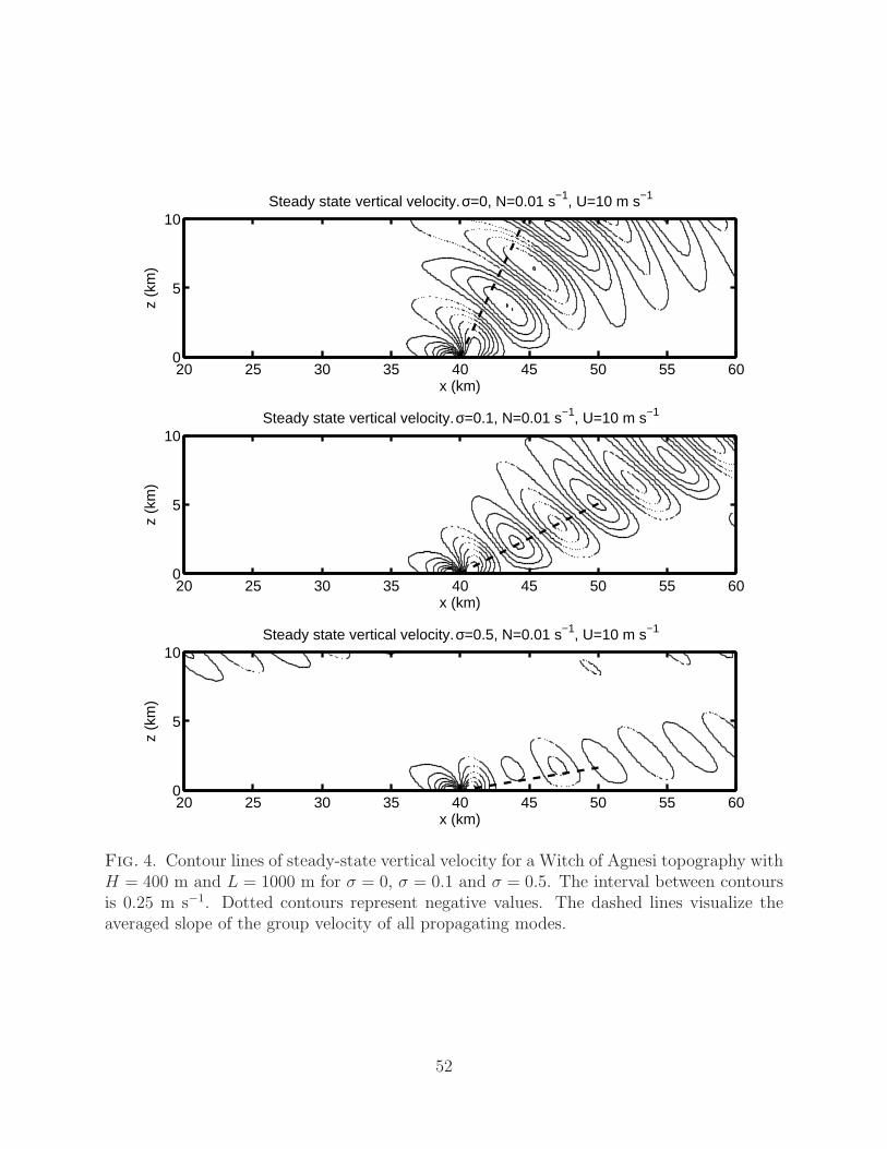
that the top of the hill is in the middle of it. Figure 4 shows solutions with Nx = 201 for
σ = 0, σ = 0.1 and σ = 0.5 for
√
θ(2)z = 1, u∞ = 0.1 or 0.01 s−1 and 10 m s−1. The
computational domain is [0, 8] × [0, 1] or [0, 80] km × [0, 10] km but the solution is plotted
only on [2, 6]× [0, 1]. Set H = 0.04 or 400 m and L = 0.1 or 1000 m.
The dashed lines visualize the average over the slopes (44) of all propagating modes,
where each mode is weighted by its amplitude. With increasing σ, the slope of the wave
pattern is reduced, according the the reduced slope of the group velocity pointed out in
3b. This is compatible with the following consideration: By decreasing the stability N of
the atmosphere, moisture increases the baroclinic Froude number Frbaroclinic, cf. (11), which
is small for waves close to hydrostatic balance. As hydrostatic waves propagate only in
the vertical and the horizontal component increases as waves become more non-hydrostatic,
it seems reasonable that an increase of Frbaroclinic by moisture leads to a reduction of the
propagation angle.
An important mechanism caused by gravity waves is the vertical transfer of horizontal
momentum. While for propagating steady-state modes the horizontally averaged vertical
flux of momentum2
ρ(0)uw (62)
is constant, for evanescent modes it decays exponentially with height. Thus by turning
propagating modes into evanescent, moisture inhibits the momentum transfer by gravity
waves. Table 1 lists the values of the horizontally averaged vertical flux of momentum at
the top of the domain for different values of σ.
2For once here, the overbar over uw denotes the horizontal average in x and not in η.
28

b. Mountain waves disturbed by a moving cloud envelope
In this subsection, we demonstrate the effect of a cloud packet being advected through
an established mountain wave pattern, so the fully time-dependent problem (1), (2) is solved
numerically. The domain is [−3, 3]×[0, 1.5] or [−30, 30] km×[0, 15] km in dimensional terms.
To realize a transparent upper boundary condition, a Rayleigh damping layer as described
in Klemp and Lilly (1978), reaching from z = 1 to z = 1.5, is used. Subsequent figures
show the solution on the subset [−2, 2] × [0, 1]. The topography is a Witch of Agnesi hill
with H = 0.04 or 400 m and L = 0.1 or 1000 m and the maximum located at x = 0. The
background flow is linearly increased from τ = 0 to τ = 0.25 up to its maximum value of
u∞ = 0.1 or 10 m s−1.
The simulation is run until τσ = 3 with σ ≡ 0. Then, a cloud packet described by a
Gaussian-distributed σ, defining its local intensity and envelope, is introduced and advected
with velocity u∞, crossing the domain and finally exiting at the right boundary. For τ ≥ τσ,
set
σ(x, z, τ) = σmax exp
(
−1
2
[
(x− xc − u∞[τ − τσ])2
s2x+
(z − zc)2
s2z
])
(63)
with sx = 0.25, sz = 0.25 and zc = 0.4. To avoid a sudden introduction of moisture at
τ = τσ, set
xc = xleft − 2 · sx with xleft = −4 (64)
so that at τσ the maximum of σ is outside the actual domain of computation at x = −4. The
cloud is then advected with velocity u∞ = 0.1 into the domain so that its maximum enters at
τ = τσ+2sxu∞
= 8 at the left boundary and would leave the domain at τ = τσ+2sxu∞
+ 6u∞
= 68.
The maximum is always located at a height of 4 km.
29

The simulation uses 300 nodes in the horizontal direction and 75 in the vertical, resulting
in a resolution of ∆x = ∆z = 0.02 or 200 m. The time step is ∆τ = 0.05 or 5 s.
The first four figures in 5 show contour lines of the vertical velocity w at different times
for a cloud envelope with σmax = 0.5. In the first figure, the cloud pattern has entered the
domain from the left. Figures two, three, and four show how the cloud envelope travels
through the mountain waves, while the last figure shows a dry reference solution at τ = 50
for comparison. Considering the third and fourth figures and comparing them with the dry
solution in figure five, we see how the cloud packet has damped the waves in the upper
region. Also in figure four a decreased propagation angle is observed.
Figure 6 shows the net vertical flux of horizontal momentum (62) over time for the dry
case, the case with σmax = 0.5 and a third simulation where only the value of σmax has been
changed to 0.2. The negative momentum flux increases towards zero as the cloud envelope
travels through the wave pattern, i.e., its magnitude is reduced as in the analysis of the
stationary solutions.
c. Waves travelling through clouds
The domain is [−5, 5]× [0, 1.25] or [−50, 50] km× [0, 12.5] km and there is no background
flow here, i.e. u∞ = 0. The stability frequency is
√
θ(2)z = 1 or 0.01 s−1. Between −30 km
to −10 km and 10 km to 30 km, two clouds packets are located.
All initial values are zero, except for a concentrated Gaussian peak of negative θ, placed
at the center of the domain with its maximum at (x, z) = (0, 0.5). Figure 7 visualizes the
distribution of σ as well as the initial θ. The simulation uses 400 nodes in the horizontal
30

direction, 40 nodes up to z = 10 km and 10 more nodes to realize the sponge layer between
z = 10 km and z = 12.5 km. The resulting resolution is ∆x = ∆z = 250 m. The time
step is ∆τ = 0.1 or 10 s. For comparison, a reference solution is computed with identical
parameters but σ ≡ 0.
The initial potential temperature perturbation starts to excite waves, which form a typical
X-shaped pattern (not shown, see for example Clark and Farley (1984)). Figure 8 shows
a cross section through the vertical velocity at 5 km of the cloudy case (continuous line)
as well as the non-cloudy reference simulation (dashed line). In the first figure, waves have
formed and started travelling outwards. Inside the cloud, the updraft from the entering wave
is amplified by latent heat release. Because the wave is also slowed down inside the cloud,
there is some steepening before the cloud. In the next figure the steepening before and the
amplification inside the cloud are even more pronounced. In the last figure one can see the
newly formed extrema and a generally strongly distorted distribution of vertical velocity
inside the cloud. In the region behind the cloud, the amplitude of the wave is noticeably
reduced compared to the non-cloudy case.
5. Conclusions
The paper presents the derivation and analysis of a model for modulation of internal
waves by deep convection. In the analysis, the dispersion relation, group velocity, and
Taylor-Goldstein equation of the extended model are computed. Moisture, represented by
the saturated area fraction σ, introduces multiple effects compared to the dry dynamics:
by altering the group velocity, it inhibits wave propagation and changes the propagation
31

direction of wave packets. It introduces a lower cut-off horizontal wavenumber below which
modes turn from propagating into evanescent. This is in contrast to the dispersion properties
of waves in a non-rotating dry atmosphere for which only an upper cut-off wavenumber exists.
The lower cut-off leads to a moisture related reduction of the vertical flux of horizontal
momentum. As gravity wave drag (GWD) is closely related to momentum flux, including
this effect in parameterizations of GWD could improve simulations, because near-hydrostatic
modes with small horizontal wavenumber, which are primarily affected by the cut-off, sig-
nificantly contribute to wave-drag. We also note that moisture can cause critical layers for
flows that would be non-critical under dry conditions.
Examples of stationary solutions obtained analytically demonstrate the cut-off, the re-
duced angle of propagation of wave packets, and the reduced momentum flux. The examples
include stationary solutions for mountain waves excited from sine shaped and Witch of Ag-
nesi topographies. The non-stationary results show how a cloud packet, represented as a
Gaussian-distributed σ, is advected through Witch of Agnesi mountain waves. A significant
damping of the waves by the cloud pattern is observed, and the reduction of momentum flux
is documented. The second example begins with a small perturbation of potential tempera-
ture between two clouds, so that the excited waves travel through them. Inside the clouds,
we observe an amplification of the amplitudes of wave-induced up- and downdrafts, while
beyond the clouds, wave-amplitudes are damped.
The derivation starts from the results in Klein and Majda (2006) and yields a model
for the interaction of non-hydrostatic internal gravity waves with a timescale of 100 s and a
lengthscale of 10 km and convective hot towers with horizontal variations on a 1 km scale.
An analytically computed closure of the model is achieved without requiring additional
32
approximations by applying weighted averages over the small 1 km horizontal scale . In the
final model, moisture is present only as a parameter σ which describes the area fraction of
saturated regions on the tower-scale.
The resulting model involves anelastic, moist, large-scale dynamics described by an ex-
tension of the linearized dry anelastic equations. The equations include a source term for the
potential temperature determined by two additional equations for the averaged dynamics on
the small tower-scale. The averaged equations for the small scales, in turn, include terms
from the large-scale dynamics so that there is bi-directional coupling between large- and
tower-scale flow components in the model.
The presented model provides some interesting possibilities for future research. The
similarity of the saturated area fraction σ with the cloud cover fraction in GCMs might
make the model a good starting point for the development of GWD parameterizations that
include moist effects. Also of interest with respect to GWD parameterizations would be
an attempt to validate the hypothesized lower horizontal cut-off wavenumber in a model
employing a full bulk micro-physics scheme. An extension of the model to the case of weak
under-saturation, in which σ will turn into a prognostic variable and the model will become
nonlinear, is work in progress.
Acknowledgments.
This research is partially funded by Deutsche Forschungsgemeinschaft, Project KL 611/14,
and by the DFG Priority Research Programs “PQP” (SSP 1167) and “MetStroem” (SPP
1276). We thank Oliver Buhler, Peter Spichtinger and Stefan Vater for helpful discussions
33

and suggestions. We also thank the three anonymous reviewers for their very helpful com-
ments on the initial version of the manuscript.
34

APPENDIX
Key steps in the derivation of the model
The non-dimensional conservation laws for mass, momentum, energy (expressed as po-
tential temperature) in Klein and Majda (2006) read
ρt +∇|| · (ρu) + (ρw)z = 0
ut + u · ∇||u+ wuz + ǫf (Ω× v)|| + ǫ−4ρ−1∇||p = 0
wt + u · ∇||w + wwz + ǫf (Ω× v)⊥ + ǫ−4ρ−1pz = −ǫ−4
θt + u · ∇||θ + wθz = ǫ2(
Sǫθ + Sq,ǫ
θ
)
(A1)
where
Sq,ǫθ = Γ∗∗L∗∗q∗∗vs
θ
p
(
ǫ−nCd − Cev
)
(A2)
is the source term related to evaporation and condensation, while Sǫθ is a given external
source of energy like, for example, radiation. Inserting (9), (15) plus the expansions of ρ, w,
p in Klein and Majda (2006) yields the following leading order equations.
35

(i) Horizontal momentum
O(ǫ2) : p(3)η = 0
O(ǫ3) : ρ(0)u(0)τ + ρ(0)u
(1)τ ′ + ρ(0)u∞u(0)
x + ρ(0)u∞u(1)η
+p(3)x + p(4)η = 0.
(A3)
The second equation can be rewritten as
ρ(0)u(0)τ + ρ(0)u∞u(0)
x + p(3)x = −[
ρ(0)u(1)τ ′ + ρ(0)u∞u(1)
η + p(4)η
]
. (A4)
By integrating this equation along a characteristic τ ′+u∞η = const. and employing sublinear
growth condition for the higher order quantities u(1) and p(4), we conclude that the right hand
side must be zero and the equation simplifies to
ρ(0)u(0)τ + ρ(0)u∞u(0)
x + p(3)x = 0. (A5)
Note that as u∞ is assumed to be constant, there is no term w(0)u∞z .
(ii) Vertical momentum
O(1) : p(0)z = −ρ(0)
O(ǫ) : p(1)z = −ρ(1)
O(ǫ2) : ρ(0)w(0)τ ′ + ρ(0)u∞w(0)
η + p(2)z = −ρ(2)
O(ǫ3) : ρ(0)w(1)τ ′ + ρ(0)u∞w(1)
η + ρ(1)w(0)τ ′ + ρ(1)u∞w(0)
η
+ρ(0)w(0)τ + ρ(0)u∞w(0)
x + ρ(0)u(0)w(0)η + p(3)z = −ρ(3)
(A6)
36

We assume ρ(1) = 0 here and employ again the sublinear growth condition. The last equation
then becomes
ρ(0)w(0)τ + ρ(0)u∞w(0)
x + ρ(0)u(0)w(0)η + p(3)z = −ρ(3). (A7)
Assuming that the specific heats cv and cp are constants and employing the Newtonian limit,
expanding the equation of state yields
−ρ(3)
ρ(0)= θ(3) − p(3)
p(0). (A8)
Using this and the hydrostatic balance for the leading order density and pressure, one obtains
w(0)τ + u∞w(0)
x + u(0)w(0)η π(3)
z = θ(3) (A9)
with π(3) := p(3)/ρ(0).
(iii) Mass
ρ(0)u(1)η + ρ(0)u(0)
x +(
ρ(0)w(0))
z= 0 (A10)
Sublinear growth yields
ρ(0)u(0)x +
(
ρ(0)w(0))
z= 0. (A11)
37
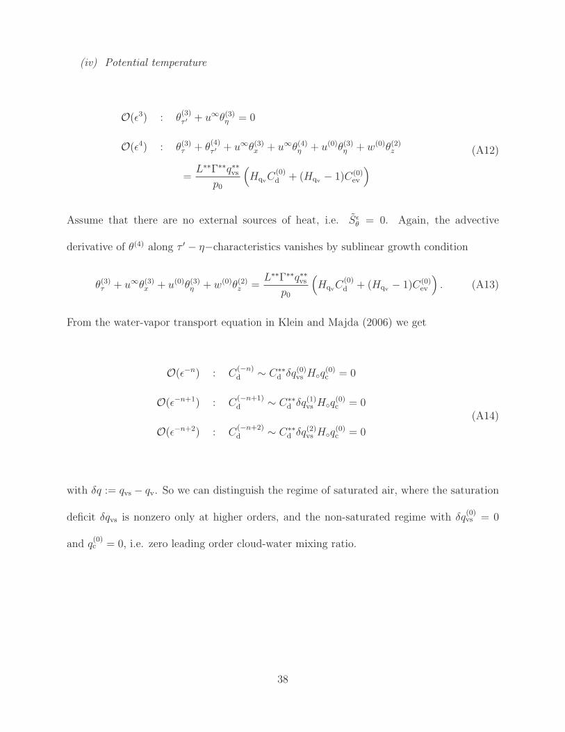
(iv) Potential temperature
O(ǫ3) : θ(3)τ ′ + u∞θ(3)η = 0
O(ǫ4) : θ(3)τ + θ(4)τ ′ + u∞θ(3)x + u∞θ(4)η + u(0)θ(3)η + w(0)θ(2)z
=L∗∗Γ∗∗q∗∗vs
p0
(
HqvC(0)d + (Hqv − 1)C(0)
ev
)
(A12)
Assume that there are no external sources of heat, i.e. Sǫθ = 0. Again, the advective
derivative of θ(4) along τ ′ − η−characteristics vanishes by sublinear growth condition
θ(3)τ + u∞θ(3)x + u(0)θ(3)η + w(0)θ(2)z =L∗∗Γ∗∗q∗∗vs
p0
(
HqvC(0)d + (Hqv − 1)C(0)
ev
)
. (A13)
From the water-vapor transport equation in Klein and Majda (2006) we get
O(ǫ−n) : C(−n)d ∼ C∗∗
d δq(0)vs Hq(0)c = 0
O(ǫ−n+1) : C(−n+1)d ∼ C∗∗
d δq(1)vs Hq(0)c = 0
O(ǫ−n+2) : C(−n+2)d ∼ C∗∗
d δq(2)vs Hq(0)c = 0
(A14)
with δq := qvs − qv. So we can distinguish the regime of saturated air, where the saturation
deficit δqvs is nonzero only at higher orders, and the non-saturated regime with δq(0)vs = 0
and q(0)c = 0, i.e. zero leading order cloud-water mixing ratio.
38
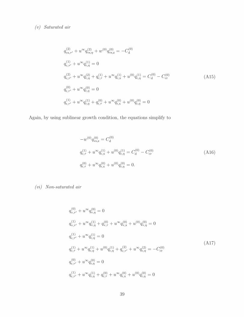
(v) Saturated air
q(2)vs,τ ′ + u∞q(2)vs,η + w(0)q(0)vs,z = −C
(0)d
q(1)c,τ ′ + u∞q(1)c,η = 0
q(2)c,τ ′ + u∞q(2)c,η + q(1)c,τ + u∞q(1)c,x + u(0)q(1)c,η = C
(0)d − C(0)
cr
q(0)r,τ ′ + u∞q(0)r,η = 0
q(1)r,τ ′ + u∞q(1)r,η + q(0)r,τ + u∞q(0)r,x + u(0)q(0)r,η = 0
(A15)
Again, by using sublinear growth condition, the equations simplify to
−w(0)q(0)vs,z = C(0)d
q(1)c,τ + u∞q(1)c,x + u(0)q(1)c,η = C(0)d − C(0)
cr
q(0)r,τ + u∞q(0)r,x + u(0)q(0)r,η = 0.
(A16)
(vi) Non-saturated air
q(0)v,τ ′ + u∞q(0)v,η = 0
q(1)v,τ ′ + u∞q(1)v,η + q(0)v,τ + u∞q(0)v,x + u(0)q(0)v,η = 0
q(1)c,τ ′ + u∞q(1)c,η = 0
q(1)c,τ + u∞q(1)c,η + u(0)q(1)c,η + q(2)c,τ ′ + u∞q(2)c,η = −C(0)
cr
q(0)r,τ ′ + u∞q(0)r,η = 0
q(1)r,τ ′ + u∞q(1)r,η + q(0)r,τ + u∞q(0)r,x + u(0)q(0)r,η = 0
(A17)
39
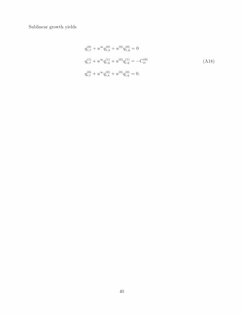
Sublinear growth yields
q(0)v,τ + u∞q(0)v,x + u(0)q(0)v,η = 0
q(1)c,τ + u∞q(1)c,η + u(0)q(1)c,η = −C(0)cr
q(0)r,τ + u∞q(0)r,x + u(0)q(0)r,η = 0.
(A18)
40

REFERENCES
Barcilon, A. and D. Fitzjarrald, 1985: A nonlinear steady model for moist hydrostatic moun-
tain waves. J. Atmos. Sci., 42, 58–67.
Barcilon, A., J. C. Jusem, and S. Blumsack, 1980: Pseudo-adiabatic flow over a two-
dimensional ridge. Geophys. Astrophys. Fluid Dynamics, 16, 19–33.
Barcilon, A., J. C. Jusem, and P. G. Drazin, 1979: On the two-dimensional, hydrostatic flow
of a stream of moist air over a mountain ridge. Geophys. Astrophys. Fluid Dynamics, 13,
125–140.
Bretherton, C. S. and P. K. Smolarkiewicz, 1989: Gravity waves, compensating subsidence
and detrainment around cumulus clouds. J. Atmos. Sci., 46, 740–759.
Buhler, O., 2009: Waves and Mean Flows. Cambrigde University Press.
Chimonas, G., F. Einaudi, and D. P. Lalas, 1980: A wave theory for the onset and initial
growth of condensation in the atmosphere. J. Atmos. Sci., 37, 827–845.
Clark, T. L. and R. D. Farley, 1984: Severe downslope windstorm calculations in two and
three spatial dimensions using anelastic interactive grid nesting: A possible mechanism
for gustiness. J. Atmos. Sci., 41, 329–350.
Davies, T., A. Staniforth, N. Wood, and J. Thuburn, 2003: Validity of anelastic and other
41
equation sets as inferred from normal-mode analysis. Q. J. R. Meteorol. Soc., 129, 2761–
2775.
Durran, D. R., 1989: Improving the anelastic approximation. J. Atmos. Sci, 46 (11), 1453–
1461.
Durran, D. R., 1991: The third-order adams-bashforth method: An attractive alternative to
leapfrog time differencing. Mon. Wea. Rev., 119, 702–720.
Durran, D. R. and J. B. Klemp, 1983: A compressible model for the simulation of moist
mountain waves. Mon. Wea. Rev., 111, 2341–2361.
Einaudi, F. and D. P. Lalas, 1973: The propagation of acoustic-gravity waves in a moist
atmosphere. J. Atmos. Sci., 30, 365–376.
Emanuel, K. A., 1994: Atmospheric Convection. Oxford University Press, 592 pp.
Etling, D., 1996: Theoretische Meteorologie. Springer, 354 pp.
Gill, A. E., 1982: Atmosphere-Ocean Dynamics. Academic Press, 662 pp.
Grabowski, W. W., 1998: Toward cloud resolving modeling of large-scale tropical circula-
tions: A simple cloud microphysics parameterization. J. Atmos. Sci., 55, 3283–3298.
Jakob, C. and S. A. Klein, 1999: The role of vertically varying cloud fraction in the pa-
rameterization of microphysical processes in the ecmwf model. Q.J.R. Meterol. Soc., 125,
941–965.
Joos, H., P. Spichtinger, U. Lohmann, J.-F. Gayet, and A. Minikin, 2008: Orographic cirrus
in the global climate model echam5. J. Geophys. Res., 113.
42

Jusem, J. C. and A. Barcilon, 1985: Simulation of moist mountain waves with an anelastic
model. Geophys. Astrophys. Fluid Dynamics, 33, 259–276.
Kim, Y.-J., S. D. Eckermann, and H.-Y. Chun, 2003: An overview of the past, present and
future of gravity-wave drag parameterization for numerical climate and weather prediction
models. Atmosphere-Ocean, 41 (1), 65–98.
Klein, R., 2009: Asymptotics, structure and integration of sound-proof atmospheric flow
equations. Theor. & Comput. Fluid Dyn., 23, 161–195.
Klein, R. and A. Majda, 2006: Systematic multiscale models for deep convection on
mesoscales. Theor. & Comput. Fluid Dyn., 20, 525–551.
Klemp, J. B. and D. K. Lilly, 1978: Numerical simulation of hydrostatic mountain waves. J.
Atmos. Sci., 35, 78–107.
Lane, T. P. and M. J. Reeder, 2001: Convectively generated gravity waves and their effect
on the cloud environment. J. Atmos. Sci., 58, 2427–2440.
LeMone, M. A. and E. J. Zipser, 1980: Cumulonimbus vertical velocity events in gate. part
i: Diameter, intensity and mass flux. J. Atmos. Sci., 37, 2444–2457.
Lighthill, J., 1978: Waves in Fluids. Cambridge University Press, 504 pp.
Lindzen, R. S., 1981: Turbulence and stress owing to gravity wave and tidal breakdown. J.
Geophys. Res., 86, 9707–9714.
Lipps, F. B. and R. S. Hemler, 1982: A scale analysis of deep moist convection and some
related numerical calculations. J. Atmos. Sci., 39, 2192–2210.
43
Majda, A. and R. Klein, 2003: Systematic multi-scale models for the tropics. J. Atmos. Sci.,
60, 393–408.
McLandress, C., 1998: On the importance of gravity waves in the middle atmosphere and
their parameterization in general circulation models. J. Atmos. Terr. Phys., 60 (14),
1357–1383.
Sawyer, J. S., 1959: The introduction of the effects of topography into methods of numerical
forecasting. Q. J. R. Meteorol. Soc., 85, 31–43.
Stevens, B., 2005: Atmospheric moist convection. Annu. Rev. Earth. Planet. Sci., 33, 605–
643.
Surgi, N., 1989: Systematic errors of the FSU global spectral model. Mon. Wea. Rev., 117,
1751–1766.
Vater, S., 2005: A new projection method for the zero froude number shallow water equa-
tions. PIK Report 97, Potsdam Institute for Climate Impact Research.
Vater, S. and R. Klein, 2009: Stability of a Cartesian grid projection method for zero Froude
number shallow water flows. Numerische Mathematik, 113 (1), 123–161.
44
List of Tables
1 Vertical flux of horizontal momentum for different values of σ in the constant
coefficient, steady-state solution. 46
45

Table 1. Vertical flux of horizontal momentum for different values of σ in the constantcoefficient, steady-state solution.
σ Momentum flux in N m−2
0 −0.710.1 −0.600.5 −0.22
46
List of Figures
1 Angle between the direction of group velocity and the horizontal for wavenum-
bers k = 1, . . . , 4 depending on σ in a steady-state flow with
√
θ(2)z = 1 or
0.01 s−1 and u∞ = 0.1 or 10 m s−1 49
2 Vertical wavelength λ for modes k = 1, . . . , 4 depending on σ for
√
θ(2)z = 1 or
0.01 s−1 and u∞ = 0.1 or 10 m s−1. The dimensional, horizontal wavelengths
corresponding to k = 1, . . . , 4 are approximately 63 km, 31 km, 21 km and
16 km. Values of σ where λ(k, σ) = 0 indicate the lower-cutoff. 50
3 Contour lines of the steady-state vertical velocity for a sine shaped topography
with horizontal wavenumber k = 2 for σ = 0, σ = 0.02 and σ = 0.05. The
interval between contours is 0.2 m s−1. Dotted contours represent negative
values. 51
4 Contour lines of steady-state vertical velocity for a Witch of Agnesi topogra-
phy with H = 400 m and L = 1000 m for σ = 0, σ = 0.1 and σ = 0.5. The
interval between contours is 0.25 m s−1. Dotted contours represent negative
values. The dashed lines visualize the averaged slope of the group velocity of
all propagating modes. 52
5 Contour lines of vertical velocity at different times for a cloud packet advected
through the waves excited by a Witch of Agnesi. Interval between contours is
0.25 m s−1 in dimensional terms. Dotted contours represent negative values.
The two thin circles are the σ = 0.05 and σ = 0.25 isoline. The last figure
shows a reference solution without any moisture at τ = 50 for comparison. 53
47
6 Net vertical flux of horizontal momentum ρ(0)uw across the height z = 10km
over time. The solid line is the dry reference simulation, the dashed line
is a moving cloud envelope with max(σ) = 0.2 while the dash-dotted line
represents a cloud envelope with max(σ) = 0.5. 54
7 σ modelling two clouds. The dashed line is the cross-section along which the
vertical velocity is plotted in figure 8. The continuous lines are isolines of σ
with a difference between isolines of 0.1 and the outer isoline corresponding
to σ = 0.1. The dotted line shows the initial distribution of θ, the difference
between the isolines is −0.025, the outer line corresponding to θ = −0.025. 55
8 Cross-section of the vertical velocity w at different times for the cloudy and
non-cloudy case. The dotted line is the cross-section through σ at the same
height, but multiplied by a factor 0.05 so that the shape is reasonably visible
in the given scaling of the y-axis. 56
48

0 0.05 0.1 0.150
0.1
0.2
0.3
0.4
σ
Ang
le in
uni
ts o
f π
Angle of group velocity depending on σ for N=0.01 s−1 , U=10 m s−1
k=1k=2k=3k=4
Fig. 1. Angle between the direction of group velocity and the horizontal for wavenumbers
k = 1, . . . , 4 depending on σ in a steady-state flow with
√
θ(2)z = 1 or 0.01 s−1 and u∞ = 0.1
or 10 m s−1
49

0 0.02 0.04 0.06 0.08 0.1 0.12 0.14 0.16 0.18 0.20
2
4
6
8
σ
λ(k,
σ) in
km
Vertical wavelength depending on σ for N=0.01 s−1, U=10 m s−1
k=1k=2k=3k=4
Fig. 2. Vertical wavelength λ for modes k = 1, . . . , 4 depending on σ for
√
θ(2)z = 1 or
0.01 s−1 and u∞ = 0.1 or 10 m s−1. The dimensional, horizontal wavelengths correspondingto k = 1, . . . , 4 are approximately 63 km, 31 km, 21 km and 16 km. Values of σ whereλ(k, σ) = 0 indicate the lower-cutoff.
50

x (km)
z (k
m)
Steady state vertical velocity. σ=0, N=0.01 s−1, U=10 m s−1
0 10 20 30 40 50 600
5
10
x (km)
z (k
m)
Steady state vertical velocity. σ=0.02, N=0.01 s−1, U=10 m s−1
0 10 20 30 40 50 600
5
10
x (km)
z (k
m)
Steady state vertical velocity. σ=0.05, N=0.01 s−1, U=10 m s−1
0 10 20 30 40 50 600
5
10
Fig. 3. Contour lines of the steady-state vertical velocity for a sine shaped topography withhorizontal wavenumber k = 2 for σ = 0, σ = 0.02 and σ = 0.05. The interval betweencontours is 0.2 m s−1. Dotted contours represent negative values.
51
x (km)
z (k
m)
Steady state vertical velocity. σ=0, N=0.01 s−1, U=10 m s−1
20 25 30 35 40 45 50 55 600
5
10
x (km)
z (k
m)
Steady state vertical velocity. σ=0.1, N=0.01 s−1, U=10 m s−1
20 25 30 35 40 45 50 55 600
5
10
x (km)
z (k
m)
Steady state vertical velocity. σ=0.5, N=0.01 s−1, U=10 m s−1
20 25 30 35 40 45 50 55 600
5
10
Fig. 4. Contour lines of steady-state vertical velocity for a Witch of Agnesi topography withH = 400 m and L = 1000 m for σ = 0, σ = 0.1 and σ = 0.5. The interval between contoursis 0.25 m s−1. Dotted contours represent negative values. The dashed lines visualize theaveraged slope of the group velocity of all propagating modes.
52

x (km)
z (k
m)
Vertical velocity at τ = 27.5, max(σ) = 0.5, N = 0.01 s−1, U=10 m s−1
−20 −15 −10 −5 0 5 10 15 200
5
10
x (km)
z (k
m)
Vertical velocity at τ = 35, max(σ) = 0.5, N = 0.01 s−1, U=10 m s−1
−20 −15 −10 −5 0 5 10 15 200
5
10
x (km)
z (k
m)
Vertical velocity at τ = 42.5, max(σ) = 0.5, N = 0.01 s−1, U=10 m s−1
−20 −15 −10 −5 0 5 10 15 200
5
10
x (km)
z (k
m)
Vertical velocity at τ = 50, max(σ) = 0.5, N = 0.01 s−1, U=10 m s−1
−20 −15 −10 −5 0 5 10 15 200
5
10
x (km)
z (k
m)
Vertical velocity at τ = 50, max(σ) = 0, N = 0.01 s−1, U=10 m s−1
−20 −15 −10 −5 0 5 10 15 200
5
10
Fig. 5. Contour lines of vertical velocity at different times for a cloud packet advectedthrough the waves excited by a Witch of Agnesi. Interval between contours is 0.25 m s−1
in dimensional terms. Dotted contours represent negative values. The two thin circles arethe σ = 0.05 and σ = 0.25 isoline. The last figure shows a reference solution without anymoisture at τ = 50 for comparison.
53

0 10 20 30 40 50 60−0.2
−0.15
−0.1
−0.05
0
τ
Mom
entu
m fl
ux in
N m
−2
Net vertical flux of horizontal momentum at z=10km
Drymax(σ)=0.2max(σ)=0.5
Fig. 6. Net vertical flux of horizontal momentum ρ(0)uw across the height z = 10km overtime. The solid line is the dry reference simulation, the dashed line is a moving cloudenvelope with max(σ) = 0.2 while the dash-dotted line represents a cloud envelope withmax(σ) = 0.5.
54
x (km)
z (k
m)
σ and initial θ
−40 −30 −20 −10 0 10 20 30 40
2
4
6
8
Fig. 7. σ modelling two clouds. The dashed line is the cross-section along which the verticalvelocity is plotted in figure 8. The continuous lines are isolines of σ with a difference betweenisolines of 0.1 and the outer isoline corresponding to σ = 0.1. The dotted line shows the initialdistribution of θ, the difference between the isolines is −0.025, the outer line correspondingto θ = −0.025.
55

−40 −30 −20 −10 0 10 20 30 40
−0.02
−0.01
0
0.01
0.02
x (km)
w (
ms−
1 )
Horizontal crossection through w at z = 5 km and τ = 5
no clouds clouds
−40 −30 −20 −10 0 10 20 30 40
−0.02
−0.01
0
0.01
0.02
x (km)
w (
ms−
1 )
Horizontal crossection through w at z = 5 km and τ = 7
no clouds clouds
−40 −30 −20 −10 0 10 20 30 40
−0.02
−0.01
0
0.01
0.02
x (km)
w (
ms−
1 )
Horizontal crossection through w at z = 5 km and τ = 9
no clouds clouds
−40 −30 −20 −10 0 10 20 30 40
−0.02
−0.01
0
0.01
0.02
x (km)
w (
ms−
1 )
Horizontal crossection through w at z = 5 km and τ = 14
no clouds clouds
Fig. 8. Cross-section of the vertical velocity w at different times for the cloudy and non-cloudy case. The dotted line is the cross-section through σ at the same height, but multipliedby a factor 0.05 so that the shape is reasonably visible in the given scaling of the y-axis.
56