module 33 – introductionteachoutcoc.org/oli_module_33_anova.pdf · 2018-08-14 · module 33 –...

The following material comes from Probability & Statistics written by the Open Learning Initiative (OLI) in conjunction with Carnegie Mellon and Stanford Universities (http://oli.cmu.edu)

Module 33 – Introduction

In the previous two modules we performed inference for one variable. More specifically, we learned about inference for the population proportion p (when the variable of interest is categorical) and inference for the population mean μ (when the variable of interest is quantitative). In the previous two modules we were also exposed to the following three forms of inference which will continue to be central as we move forward in the course:

• Point estimation—estimating an unknown parameter with a single value that is computed from the sample.

• Interval estimation—estimating an unknown parameter by an interval of plausible values. To each such interval we attach a level of confidence that indeed the interval captures the value of the unknown parameter and hence the name confidence intervals.

• Hypothesis testing—a four-step process in which we are assessing evidence provided by the data in favor or against some claim about the population parameter.

Our next (and final) goal for this course is to perform inference about relationships between two variables in a population, based on an observed relationship between variables in a sample. Here is what the process looks like:

We are interested in studying whether a relationship exists between the variables X and Y in a population of interest. We choose a random sample and collect data on both variables from the subjects. Our goal is to determine whether these data provide strong enough evidence for us to generalize the observed relationship in the sample and conclude (with some acceptable and agreed-upon level of uncertainty) that a relationship between X and Y exists in the entire population.

The primary inference form that we will use in this module, then, is hypothesis testing. Conceptually, across all the inferential methods that we will learn, we'll test some form of:


(We will also discuss point and interval estimation, but our discussion about these forms of inference will be framed around the test.)

Recall that in the module about examining the relationship between two variables in the Exploratory Data Analysis unit, our discussion was framed around the role-type classification table. This part of the course will be structured exactly in the same way.

In other words, we will go through 3 sections corresponding to cases C→Q, C→C, and Q→Q in the table below.

(Recall that case Q→C is not discussed in this course.)

In total, we will introduce 5 inferential methods: three in case C→Q (corresponding to a division of this case into 3 sub-cases) and one in each of the cases C→C and Q→Q.

Unlike the previous part of the course on Inference for One Variable, where we discussed in some detail the theory behind the machinery of the test (such as the null distribution of the test statistic, under which the p-values are calculated), in the 5 inferential procedures that we will introduce in Inference for Relationships, we will discuss much less of that kind of detail. The principles are the same, but the details behind the null distribution of the test statistic (under which the p-value is calculated) become more complicated and require knowledge of theoretical results that are definitely beyond the scope of this course.

Instead, within each of the five inferential methods we will focus on:

• When the inferential method is appropriate for use.


• Under what conditions the procedure can safely be used. • The conceptual idea behind the test (as it is usually captured by the test statistic). • How to use software to carry out the procedure in order to get the p-value of the test. • Interpreting the results in the context of the problem.

Also, we will continue to introduce each test according to the four-step process of hypothesis testing. We are now ready to start with Case C→Q.

Content by the Open Learning Initiative and licensed under CC BY-NC-SA 3.0.

Module 33 - Case C→Q (1 of 2)

Recall the role-type classification table framing our discussion on inference about the relationship between two variables.

We start with case C→Q, where the explanatory variable is categorical and the response variable is quantitative. Recall that in the Exploratory Data Analysis unit, examining the relationship between X and Y in this case amounts, in practice, to comparing the distributions of the (quantitative) response Y for each value (category) of the explanatory X. To do that, we used side-by-side boxplots (each representing the distribution of Y in one of the groups defined by X), and supplemented the display with the corresponding descriptive statistics.

https://oli.cmu.edu/

https://creativecommons.org/licenses/by-nc-sa/3.0/


What will we do in inference? To understand the logic, we'll start with an example and then generalize.

EXAMPLE

GPA and Year in College

Say that our variable of interest is the GPA of college students in the United States. From the previous module we know that since GPA is quantitative, we do inference on μ, the (population) mean GPA among all U.S. college students. Since this module is about relationships, let's assume that what we are really interested in is not simply GPA, but the relationship between:

X : year in college (1 = freshmen, 2 = sophomore, 3 = junior, 4 = senior) and

Y : GPA

In other words, we want to explore whether GPA is related to year in college. The way to think about this is that the population of U.S. college students is now broken into 4 sub-populations: freshmen, sophomores, juniors and seniors. Within each of these four groups, we are interested in the GPA.

The inference must therefore involve the 4 sub-population means:

μ1 : mean GPA among freshmen in the United States.

μ2 : mean GPA among sophomores in the United States

μ3 : mean GPA among juniors in the United States

μ4 : mean GPA among seniors in the United States

It makes sense that the inference about the relationship between year and GPA has to be based on some kind of comparison of these four means. If we infer that these four means are not all equal (i.e., that there are some differences in GPA across years in college) then that's equivalent to saying GPA is related to year in college. Let's summarize this example with a figure:


In general, then, making inferences about the relationship between X and Y in Case C→Q boils down to comparing the means of Y in the sub-populations, which are created by the categories defined in X (say k categories). The following figure summarizes this:


As the introduction to this module mentioned, we will learn three inferential methods in Case C→Q, corresponding to a sub-division of this case. First we will distinguish between cases where the explanatory X has only two categories (k = 2), and cases where X has more than two categories (k > 2). In other words, we will look separately at cases where we are comparing two sub-population means:


and cases where we are comparing more than 2 sub-population means:


For example, if we are interested in whether GPA (Y) is related to gender (X), this is a case where k = 2(since gender has only two categories: M, F), and the inference will boil down to comparing the mean GPA in the sub-population of males to that in the sub-population of females. On the other hand, in the example we looked at earlier, the relationship between GPA (Y) and year (X) is a case where k > 2 or more specifically, k = 4 (since year has four categories). In terms of inference, these two examples will be treated differently!





Module 33 - Case C→Q (2 of 2)

Furthermore, within the sub-case of comparing two means (i.e., examining the relationship between X and Y, when X has only two categories) we will distinguish between two (sub-sub) cases. Here, the distinction is somewhat subtle, and has to do with how the samples from each of the two sub-populations we're comparing are chosen. In other words, what study design will be implemented. We have learned that many experiments, as well as observational studies, make a comparison between two groups (sub-populations) in order to see how responses differ for the two possible categorical values. In some cases, one group (sub-population 1) has one categorical value, and another independent group (sub-population 2) has the other value. Independent samples are then taken from each group for comparison.

In other cases, a matched pairs sample design may be used, where each observation in one sample is matched/paired/linked with an observation in the other sample. These are sometimes called "dependent samples."


Matching could be by person (if the same person is measured twice), or could actually be a pair of individuals who belong together in a relevant way (husband and wife, siblings). In this design, then, the same individual or a matched pair of individuals is used to make two measurements of the response—one for each of the two categorical values.

Comment

Note that in the first figure, where the samples are independent, the sample sizes of the two independent samples need not be the same (and thus we used n1 and n2 to indicate the two sample sizes). On the other hand, it is obvious from the design that in the matched pairs the sample sizes of the two samples must be the same (and thus we used n for both).

EXAMPLE

The department of motor vehicles wants to check whether drivers are impaired after drinking two beers. Consider the following two designs:

1. The reaction times (measured in seconds) in an obstacle course are measured for a group of 10 drivers who had no beer. Two beers are given to each of a different group of 9 drivers, and their reaction times on the same obstacle course are measured. (In practice, this was done by selecting a random sample of 19 drivers and randomly assigning them to one of the two groups. The random assignment guarantees, at least in theory, that the two groups are independent).


2. The reaction times (measured in seconds) in an obstacle course are measured for 8 randomly selected drivers before and then after the consumption of two beers.


In the first design, we have two independent samples, and the second design is a matched-pairs design, since each individual was measured twice, once before and once after. The two figures highlight the main difference between the two designs. As we'll see, when we have two independent samples, the comparison of the reaction times is a comparison between two groups. In matched pairs, the comparison between the reaction times is done for each individual.


Module 33 - ANOVA ( 1 of 7)

Comparing More Than Two Means—ANOVA Overview

In this part, we continue to handle situations involving one categorical explanatory variable and one quantitative response variable, which is case C→Q in our role/type classification table:




So far we have discussed the two samples and matched pairs designs, in which the categorical explanatory variable is two-valued. As we saw, in these cases, examining the relationship between the explanatory and the response variables amounts to comparing the mean of the response variable (Y) in two populations, which are defined by the two values of the explanatory variable (X). The difference between the two samples and matched pairs designs is that in the former, the two samples are independent, and in the latter, the samples are dependent.

We are now moving on to cases in which the categorical explanatory variable takes more than two values. Here, as in the two-valued case, making inferences about the relationship between the explanatory (X) and the response (Y) variables amounts to comparing the means of the response variable in the populations defined by the values of the explanatory variable, where the number of means we are comparing depends, of course, on the number of values of X. Unlike the two-valued case, where we looked at two sub-cases (1) when the samples are independent (two samples design) and (2) when the samples are dependent (matched pairs design, here, we are just going to discuss the case where the samples are independent. In other words, we are just going to extend the two samples design to more than two independent samples.


Comment

The extension of the matched pairs design to more than two dependent samples is called "Repeated Measures" and is beyond the scope of this course.

The inferential method for comparing more than two means that we will introduce in this part is called Analysis Of Variance (abbreviated as ANOVA), and the test associated with this method is called the ANOVA F-test. The structure of this part will be very similar to that of the previous two. We will first present our leading example, and then introduce the ANOVA F-test by going through its 4 steps, illustrating each one using the example. (It will become clear as we explain the idea behind the test where the name "Analysis of Variance" comes from.) We will then present another complete example, and conclude with some comments about possible follow-ups to the test. As usual, you'll have activities along the way to check your understanding, and learn how to use software to carry out the test.

Let's start by introducing our leading example.

EXAMPLE

Is "academic frustration" related to major?


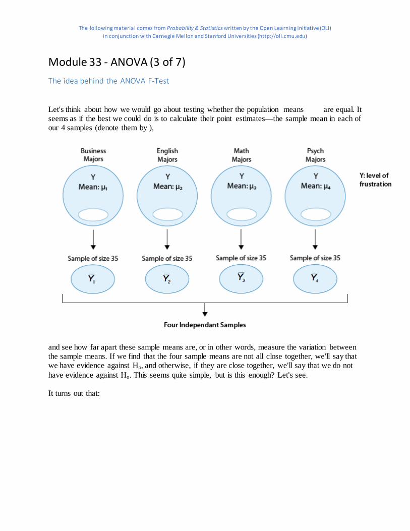
A college dean believes that students with different majors may experience different levels of academic frustration. Random samples of size 35 of Business, English, Mathematics, and Psychology majors are asked to rate their level of academic frustration on a scale of 1 (lowest) to 20 (highest).

The figure highlights what we have already mentioned: examining the relationship between major (X) and frustration level (Y) amounts to comparing the mean frustration levels (μ1,μ2,μ3,μ4μ1,μ2,μ3,μ4 ) among the four majors defined by X. Also, the figure reminds us that we are dealing with a case where the samples are independent.

Comment

There are two ways to record data in the ANOVA setting:

• Unstacked: One column for each of the four majors, with each column listing the frustration levels reported by all sampled students in that major:


• Stacked: one column for all the frustration levels, and next to it a column to keep track of which major a student is in:

The "unstacked" format helps us to look at the four groups separately, while the "stacked" format helps us remember that there are, in fact, two variables involved: frustration level (the quantitative response variable) and major (the categorical explanatory variable).


Module 33 - ANOVA (2 of 7)




EXAMPLE

Recall our "Is academic frustration related to major?" example:


The correct hypotheses for our example are:

Before we move on to the next step (checking conditions and summarizing the data with a test statistic), we will present the idea behind the ANOVA F-test using our example.





Module 33 - ANOVA (3 of 7) The idea behind the ANOVA F-Test

Let's think about how we would go about testing whether the population means are equal. It seems as if the best we could do is to calculate their point estimates—the sample mean in each of our 4 samples (denote them by ),

and see how far apart these sample means are, or in other words, measure the variation between the sample means. If we find that the four sample means are not all close together, we'll say that we have evidence against Ho, and otherwise, if they are close together, we'll say that we do not have evidence against Ho. This seems quite simple, but is this enough? Let's see.

It turns out that:


Below we present two possible scenarios for our example. In both cases, we construct side-by-side boxplots for four groups of frustration levels that have the same variation among their means. Thus, Scenario #1 and Scenario #2 both show data for four groups with the sample means 7.3, 11.8, 13.2, and 14.0 (indicated with red marks).


The important difference between the two scenarios is that the first represents data with a large amount of variation within each of the four groups; the second represents data with a small amount of variation within each of the four groups.


Scenario 1, because of the large amount of spread within the groups, shows boxplots with plenty of overlap. One could imagine the data arising from 4 random samples taken from 4 populations, all having the same mean of about 11 or 12. The first group of values may have been a bit on the low side, and the other three a bit on the high side, but such differences could conceivably have come about by chance. This would be the case if the null hypothesis, claiming equal population means, were true. Scenario 2, because of the small amount of spread within the groups, shows boxplots with very little overlap. It would be very hard to believe that we are sampling from four groups that have equal population means. This would be the case if the null hypothesis, claiming equal population means, were false.

Thus, in the language of hypothesis tests, we would say that if the data were configured as they are in scenario 1, we would not reject the null hypothesis that population mean frustration levels were equal for the four majors. If the data were configured as they are in scenario 2, we would reject the null hypothesis, and we would conclude that mean frustration levels differ, depending on major.

Let's summarize what we learned from this. The question we need to answer is: Are the

differences among the sample means ( ) due to true differences among the μ's (alternative hypothesis), or merely due to sampling variability (null hypothesis)?

In order to answer this question using our data, we obviously need to look at the variation among the sample means, but this alone is not enough. We need to look at the variation among the sample means relative to the variation within the groups. In other words, we need to look at the quantity:

which measures to what extent the difference among the sampled groups' means dominates over the usual variation within sampled groups (which reflects differences in individuals that are typical in random samples).

When the variation within groups is large (like in scenario 1), the variation (differences) among the sample means could become negligible and the data provide very little evidence against Ho. When the variation within groups is small (like in scenario 2), the variation among the sample means dominates over it, and the data have stronger evidence against Ho.

Looking at this ratio of variations is the idea behind the comparing more than two means; hence the name analysis of variance (ANOVA).

Now that we understand the idea behind the ANOVA F-test, let's move on to step 2. We'll start by talking about the test statistic, since it will be a natural continuation of what we've just


discussed, and then move on to talk about the conditions under which the ANOVA F-test can be used. In practice, however, the conditions need to be checked first, as we did before.


Module 33 - ANOVA (4 of 7) Step 2: Checking Conditions and Finding the Test Statistic

The test statistic of the ANOVA F-test, called the F statistic, has the form

It has a different structure from all the test statistics we've looked at so far, but it is similar in that it is still a measure of the evidence against H0. The larger F is (which happens when the denominator, the variation within groups, is small relative to the numerator, the variation among the sample means), the more evidence we have against H0.

Comments

1. The focus here is for you to understand the idea behind this test statistic, so we do not go into detail about how the two variations are measured. We instead rely on software output to obtain the F-statistic.

2. This test is called the ANOVA F-test. So far, we have explained the ANOVA part of the name. Based on the previous tests we introduced, it should not be surprising that the "F-test" part comes from the fact that the null distribution of the test statistic, under which the p-values are calculated, is called an F-distribution. We will say very little about the F-distribution in this course, which will essentially be limited to this comment and the next one.

3. It is fairly straightforward to decide if a z-statistic is large. Even without tables, we should realize by now that a z-statistic of 0.8 is not especially large, whereas a z-statistic of 2.5 is large. In the case of the t-statistic, it is less straightforward, because there is a different t-distribution for every sample size n (and degrees of freedom n − 1). However, the fact that a t-distribution with a large number of degrees of freedom is very close to the z (standard normal) distribution can help to assess the magnitude of the t-test statistic.




When the size of the F-statistic must be assessed, the task is even more complicated, because there is a different F-distribution for every combination of the number of groups we are comparing and the total sample size. We will nevertheless say that for most situations, an F-statistic greater than 4 would be considered rather large, but tables or software are needed to get a truly accurate assessment.

EXAMPLE

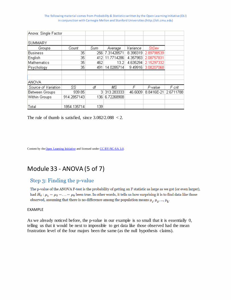
The parts of the output that we focus on here have been highlighted. In particular, note that the F-statistic is 46.60, which is very large, indicating that the data provide a lot of evidence against H0 (we can also see that the p-value is so small that it is essentially 0, which supports that conclusion as well).

Let's move on to talk about the conditions under which we can safely use the ANOVA F-test, where the first two conditions are very similar to ones we've seen before, but there is a new third condition. It is safe to use the ANOVA procedure when the following conditions hold:

1. The samples drawn from each of the populations we're comparing are independent. 2. The response variable varies normally within each of the populations we're comparing.

As you already know, in practice this is done by looking at the histograms of the samples and making sure that there is no evidence of extreme departure from normality in the form of extreme skewness and outliers. Another possibility is to look at side-by-side boxplots of the data, and add histograms if a more detailed view is necessary. For large sample sizes, we don't really need to worry about normality, although it is always a good idea to look at the data.

3. The populations all have the same standard deviation. The best we can do to check this condition is to find the sample standard deviations of our samples and check whether they are "close." A common rule of thumb is to check whether the ratio between the largest sample standard deviation and the smallest is less than 2. If that's the case, this condition is considered to be satisfied.


EXAMPLE

In our example all the conditions are satisfied:

1. All the samples were chosen randomly, and are therefore independent. 2. The sample sizes are large enough (n = 35) that we really don't have to worry about the

normality; however, let's look at the data using side-by-side boxplots, just to get a sense of it:

You'll recognize this plot as Scenario 2 from earlier. The data suggest that the frustration level of the business students is generally lower than students from the other three majors. The ANOVA F-test will tell us whether these differences are significant.

3. In order to use the rule of thumb, we need to get the sample standard deviations of our samples.

We can either calculate the standard deviation for each of the four samples by hand, or note that the variance for each sample appears in the Excel output and use that to calculate the standard deviation (remember that the square root of variance is standard deviation). Here, the standard deviation has been calculated and added to the output:


The rule of thumb is satisfied, since 3.082/2.088 < 2.



EXAMPLE

As we already noticed before, the p-value in our example is so small that it is essentially 0, telling us that it would be next to impossible to get data like those observed had the mean frustration level of the four majors been the same (as the null hypothesis claims).




Step 4: Making Conclusions in Context

As usual, we base our conclusion on the p-value. A small p-value tells us that our data contain a lot of evidence against Ho. More specifically, a small p-value tells us that the differences between the sample means are statistically significant (unlikely to have happened by chance), and therefore we reject Ho. If the p-value is not small, the data do not provide enough evidence to reject Ho, and so we continue to believe that it may be true. A significance level (cut-off probability) of .05 can help determine what is considered a small p-value.

EXAMPLE

In our example, the p-value is extremely small—close to 0—indicating that our data provide extremely strong evidence to reject Ho. We conclude that the frustration level means of the four majors are not all the same, or in other words, that majors do have an effect on students' academic frustration levels at the school where the test was conducted.






Before we give you hands-on practice in carrying out the ANOVA F-test, let's look at another example:

EXAMPLE

Do advertisers alter the reading level of their ads based on the target audience of the magazine they advertise in?

In 1981, a study of magazine advertisements was conducted (F.K. Shuptrine and D.D. McVicker, "Readability Levels of Magazine Ads," Journal of Advertising Research, 21:5, October 1981). Researchers selected random samples of advertisements from each of three groups of magazines:

Group 1—highest educational level magazines (such as Scientific American, Fortune, The New Yorker)

Group 2—middle educational level magazines (such as Sports Illustrated, Newsweek, People)

Group 3—lowest educational level magazines (such as National Enquirer, Grit, True Confessions)

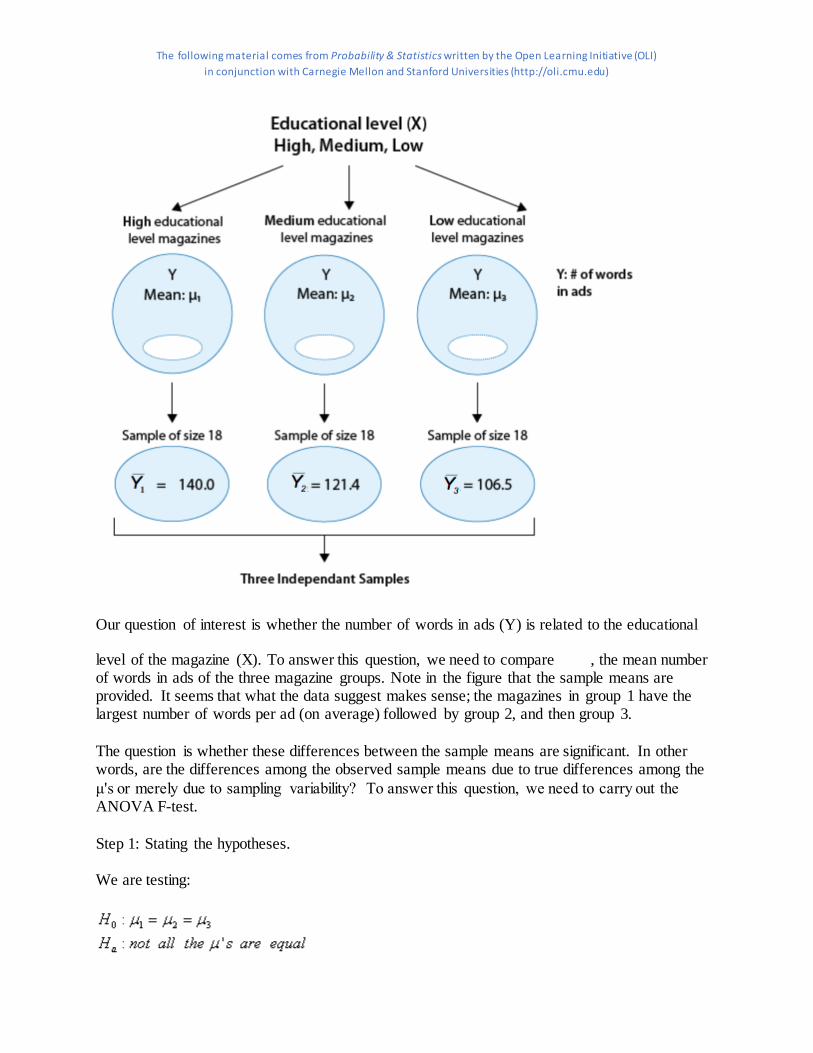
The measure that the researchers used to assess the level of the ads was the number of words in the ad. 18 ads were randomly selected from each of the magazine groups, and the number of words per ad were recorded.

The following figure summarizes this problem:


Our question of interest is whether the number of words in ads (Y) is related to the educational

level of the magazine (X). To answer this question, we need to compare , the mean number of words in ads of the three magazine groups. Note in the figure that the sample means are provided. It seems that what the data suggest makes sense; the magazines in group 1 have the largest number of words per ad (on average) followed by group 2, and then group 3.

The question is whether these differences between the sample means are significant. In other words, are the differences among the observed sample means due to true differences among the μ's or merely due to sampling variability? To answer this question, we need to carry out the ANOVA F-test.

Step 1: Stating the hypotheses.

We are testing:


Conceptually, the null hypothesis claims that the number of words in ads is not related to the educational level of the magazine, and the alternative hypothesis claims that there is a relationship.

Step 2: Checking conditions and summarizing the data.

(i) The ads were selected at random from each magazine group, so the three samples are independent.

In order to check the next two conditions, we'll need to look at the data (condition ii), and calculate the sample standard deviations of the three samples (condition iii). Here are the side-by-side boxplots of the data, followed by the standard deviations:

(ii) The graph does not display any alarming violations of the normality assumption. It seems like there is some skewness in groups 2 and 3, but not extremely so, and there are no outliers in the data.

(iii) We can assume that the equal standard deviation assumption is met since the rule of thumb is satisfied: the largest sample standard deviation of the three is 74 (group 1), the smallest one is 57.6 (group 3), and 74/57.6 < 2.


Before we move on, let's look again at the graph. It is easy to see the trend of the sample means (indicated by red circles). However, there is so much variation within each of the groups that there is almost a complete overlap between the three boxplots, and the differences between the means are over-shadowed and seem like something that could have happened just by chance. Let's move on and see whether the ANOVA F-test will support this observation.

Using statistical software to conduct the ANOVA F-test, we find that the F statistic is 1.18, which is not very large. We also find that the p-value is 0.317.

Step 3. Finding the p-value.

The p-value is 0.317, which tells us that getting data like those observed is not very surprising assuming that there are no differences between the three magazine groups with respect to the mean number of words in ads (which is what Ho claims).

In other words, the large p-value tells us that it is quite reasonable that the differences between the observed sample means could have happened just by chance (i.e., due to sampling variability) and not because of true differences between the means.

Step 4: Making conclusions in context.

The large p-value indicates that the results are not significant, and that we cannot reject Ho.

We therefore conclude that the study does not provide evidence that the mean number of words in ads is related to the educational level of the magazine. In other words, the study does not provide evidence that advertisers alter the reading level of their ads (as measured by the number of words) based on the educational level of the target audience of the magazine.





EXAMPLE

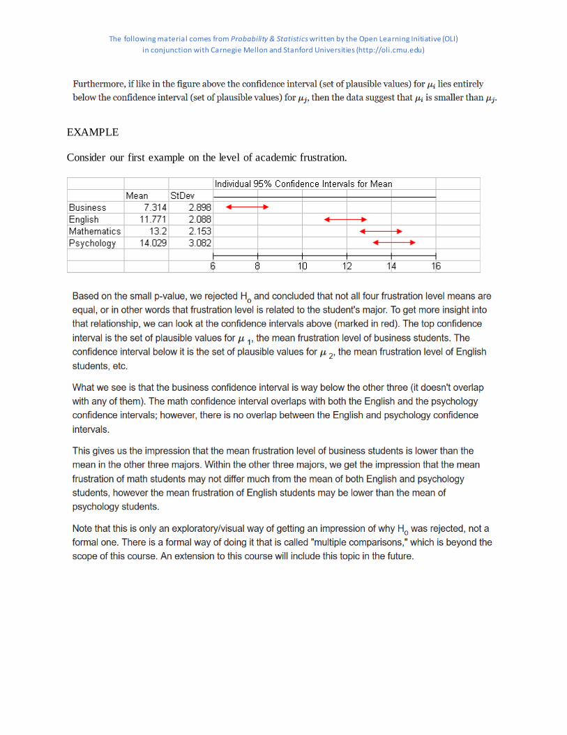
Consider our first example on the level of academic frustration.

module 33 – introductionteachoutcoc.org/oli_module_33_anova.pdf · 2018-08-14 · module 33 –...

Documents