module p2.1 introducing motion
TRANSCRIPT
F L E X I B L E L E A R N I N G A P P R O A C H T O P H Y S I C S
FLAP P2.1 Introducing motionCOPYRIGHT © 1998 THE OPEN UNIVERSITY S570 V1.1
Module P2.1 Introducing motion1 Opening items
1.1 Module introduction
1.2 Fast track questions
1.3 Ready to study?
2 Position, displacement and motion
2.1 Positions and position vectors
2.2 Displacement and distance
2.3 Linear motion
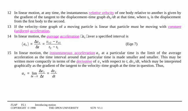
2.4 Position–time and displacement–time graphs
3 Velocity and speed
3.1 Constant velocity and constant speed
3.2 Average velocity
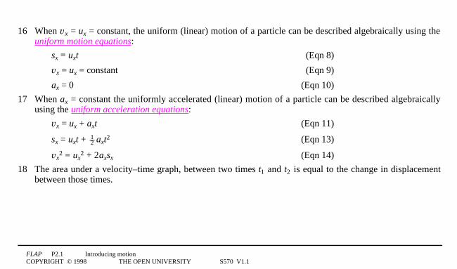
3.3 Instantaneous velocity
4 Acceleration
4.1 Constant acceleration
4.2 Average acceleration
4.3 Instantaneous acceleration
5 Equations of motion
5.1 Uniform motion equations
5.2 Uniform acceleration equations
5.3 Solution to the introductory problem
6 Closing items
6.1 Module summary
6.2 Achievements
6.3 Exit test
Exit module
FLAP P2.1 Introducing motionCOPYRIGHT © 1998 THE OPEN UNIVERSITY S570 V1.1
1 Opening items1.1 Module introductionMany of the most interesting problems in physics involve motion; the movement of planets and satellites forexample, or the motion of high speed electrons as they are whirled around in a particle accelerator. This moduleprovides an introduction to the study of motion. Its main aim is to enable you to describe and analyse simpleexamples of motion in an exact and concise way.
The module starts with a brief discussion of three-dimensional space and the way in which a Cartesiancoordinate system can be used to fix the location of an object in space. During this discussion position,displacement and distance are defined and the distinction between a vector and a scalar is explained. Havingestablished the three-dimensional nature of space and the difficulties of working in three dimensions, Subsection2.3 introduces the simplifying concept of linear motion, i.e. motion along a straight line. By concentrating in therest of the module on examples of linear motion, such as objects falling under gravity or cars accelerating alongstraight roads, we are able to explore some of the fundamental features of motion in a one-dimensional context,without having to make use of vectors. In particular, we show how position–time graphs can be used to describelinear motion. By considering such graphs we are led, in Section 3, to important concepts such as uniformmotion, average velocity and instantaneous velocity.
FLAP P2.1 Introducing motionCOPYRIGHT © 1998 THE OPEN UNIVERSITY S570 V1.1
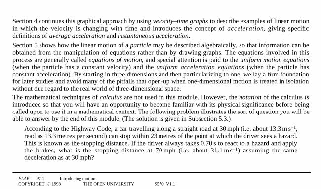
Section 4 continues this graphical approach by using velocity–time graphs to describe examples of linear motionin which the velocity is changing with time and introduces the concept of acceleration, giving specificdefinitions of average acceleration and instantaneous acceleration.
Section 5 shows how the linear motion of a particle may be described algebraically, so that information can beobtained from the manipulation of equations rather than by drawing graphs. The equations involved in thisprocess are generally called equations of motion, and special attention is paid to the uniform motion equations(when the particle has a constant velocity) and the uniform acceleration equations (when the particle hasconstant acceleration). By starting in three dimensions and then particularizing to one, we lay a firm foundationfor later studies and avoid many of the pitfalls that open-up when one-dimensional motion is treated in isolationwithout due regard to the real world of three-dimensional space.The mathematical techniques of calculus are not used in this module. However, the notation of the calculus isintroduced so that you will have an opportunity to become familiar with its physical significance before beingcalled upon to use it in a mathematical context. The following problem illustrates the sort of question you will beable to answer by the end of this module. (The solution is given in Subsection 5.3.)
According to the Highway Code, a car travelling along a straight road at 301mph (i.e. about 13.31m1s−1,read as 13.31metres per second) can stop within 231metres of the point at which the driver sees a hazard.This is known as the stopping distance. If the driver always takes 0.701s to react to a hazard and applythe brakes, what is the stopping distance at 701mph (i.e. about 31.11m1s−1) assuming the samedeceleration as at 301mph?
FLAP P2.1 Introducing motionCOPYRIGHT © 1998 THE OPEN UNIVERSITY S570 V1.1
Study comment Having read the introduction you may feel that you are already familiar with the material covered by thismodule and that you do not need to study it. If so, try the Fast track questions given in Subsection 1.2. If not, proceeddirectly to Ready to study? in Subsection 1.3.
FLAP P2.1 Introducing motionCOPYRIGHT © 1998 THE OPEN UNIVERSITY S570 V1.1
1.2 Fast track questions
Study comment Can you answer the following Fast track questions?. If you answer the questions successfully you needonly glance through the module before looking at the Module summary (Subsection 6.1) and the Achievements listed inSubsection 6.2. If you are sure that you can meet each of these achievements, try the Exit test in Subsection 6.3. If you havedifficulty with only one or two of the questions you should follow the guidance given in the answers and read the relevantparts of the module. However, if you have difficulty with more than two of the Exit questions you are strongly advised tostudy the whole module.
Question F1
A car accelerates uniformly along a straight road, so that its speed increases from 151m1s−1 to 251m1s−1 in 9.01s.Calculate its acceleration.
FLAP P2.1 Introducing motionCOPYRIGHT © 1998 THE OPEN UNIVERSITY S570 V1.1
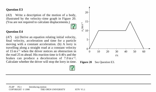
1 2 3 4 5 6 7 8 9 10t/s
50
v x/m
1s−
1
40
30
20
10
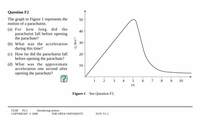
Figure 13See Question F2.
Question F2
The graph in Figure 1 represents themotion of a parachutist.
(a) For how long did theparachutist fall before openingthe parachute?
(b) What was the accelerationduring this time?
(c) How far did the parachutist fallbefore opening the parachute?
(d) What was the approximateacceleration one second afteropening the parachute?
FLAP P2.1 Introducing motionCOPYRIGHT © 1998 THE OPEN UNIVERSITY S570 V1.1
Question F3
What is the difference between a vector and a scalar? What is meant by the magnitude of a vector, and what iswrong with the statement |1a1| = –3?
Study comment
Having seen the Fast track questions you may feel that it would be wiser to follow the normal route through the module andto proceed directly to Ready to study? in Subsection 1.3.
Alternatively, you may still be sufficiently comfortable with the material covered by the module to proceed directly to theClosing items.
FLAP P2.1 Introducing motionCOPYRIGHT © 1998 THE OPEN UNIVERSITY S570 V1.1
1.3 Ready to study?
Study comment To begin to study this module you will need to be familiar with the following terms: axes, Cartesiancoordinates, gradient of a line, graph, origin, SI units and tangent. If you are unsure of any of these terms you should refer tothe Glossary, which will also indicate where in FLAP they are developed. The following questions will establish whether youneed to review some of these topics before beginning to work through this module.
FLAP P2.1 Introducing motionCOPYRIGHT © 1998 THE OPEN UNIVERSITY S570 V1.1
4
y
2
2 4 6x
0
6
8
8
A
B
Figure 23See Question R1.
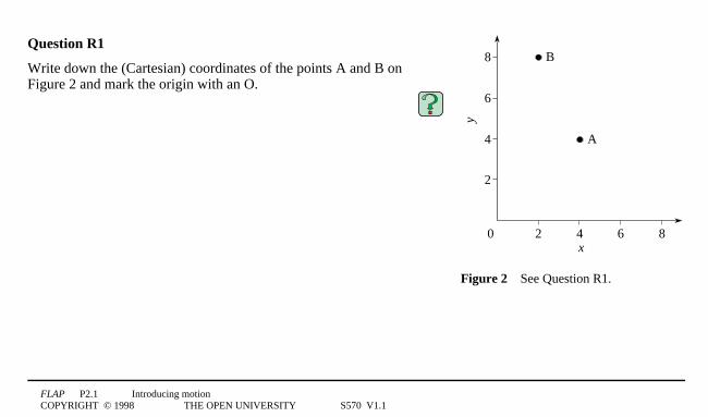
Question R1
Write down the (Cartesian) coordinates of the points A and B on Figure 2 and mark the origin with an O.
FLAP P2.1 Introducing motionCOPYRIGHT © 1998 THE OPEN UNIVERSITY S570 V1.1
0.5 1.0
50
100
150
200
cost / pence
mass of sugar / kg500 1000
10
11
12
13
temperature / °C
altitude / m
90
Figure 33See Question R2.
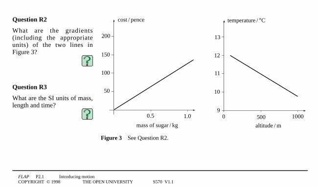
Question R2
What are the gradients(including the appropriateunits) of the two lines inFigure 3?
Question R3
What are the SI units of mass,length and time?
FLAP P2.1 Introducing motionCOPYRIGHT © 1998 THE OPEN UNIVERSITY S570 V1.1
2 Position, displacement and motion
origin
z
y
x
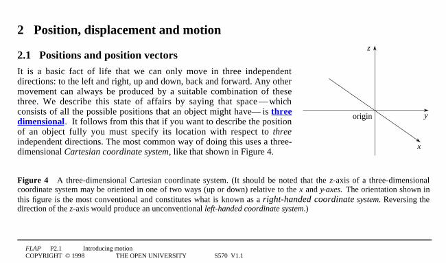
2.1 Positions and position vectorsIt is a basic fact of life that we can only move in three independentdirections: to the left and right, up and down, back and forward. Any othermovement can always be produced by a suitable combination of thesethree. We describe this state of affairs by saying that space1—1whichconsists of all the possible positions that an object might have—1is threedimensional. It follows from this that if you want to describe the positionof an object fully you must specify its location with respect to threeindependent directions. The most common way of doing this uses a three-dimensional Cartesian coordinate system, like that shown in Figure 4.
Figure 43A three-dimensional Cartesian coordinate system. (It should be noted that the z-axis of a three-dimensionalcoordinate system may be oriented in one of two ways (up or down) relative to the x and y-axes. The orientation shown inthis figure is the most conventional and constitutes what is known as a right-handed coordinate system. Reversing thedirection of the z-axis would produce an unconventional left-handed coordinate system.)
FLAP P2.1 Introducing motionCOPYRIGHT © 1998 THE OPEN UNIVERSITY S570 V1.1
z/m
3
2
y/m21
−2−3
−2 −1
−2
−1
P
x/m
1
3
1 = zP
−1
yP = −3
m, 13coordinates of P = (2 m, − m)
2 = xP
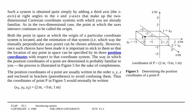
Figure 53Determining the positioncoordinates of a point P.
Such a system is obtained quite simply by adding a third axis (the z-axis) at right angles to the x and y-axes that make up the two-dimensional Cartesian coordinate systems with which you are alreadyfamiliar. As in the two-dimensional case, the point at which the axesintersect continues to be called the origin.
Both the point in space at which the origin of a particular coordinatesystem is located, and the orientation of that system (i.e. which way themutually perpendicular axes point) can be chosen arbitrarily. However,once such choices have been made it is important to stick to them so thatthe location of any point in space can be specified by its three positioncoordinates with respect to that coordinate system. The way in whichthe position coordinates of a point are determined is probably familiar toyou1—1the process is illustrated in Figure 5 for the sake of completeness.
The position coordinates of a point are usually written in the order x, y, zand enclosed in brackets (parentheses) to avoid confusing them. Thusthe coordinates of point P in Figure 5 would normally be written
(xP, yP, zP) = (21m, −31m, 11m)
FLAP P2.1 Introducing motionCOPYRIGHT © 1998 THE OPEN UNIVERSITY S570 V1.1
z
P
zP
y
x
yP
rP
xP
Figure 63The position vector rP of apoint P.
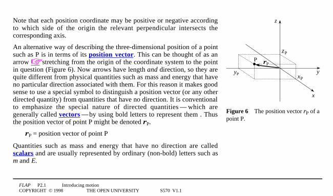
Note that each position coordinate may be positive or negative accordingto which side of the origin the relevant perpendicular intersects thecorresponding axis.
An alternative way of describing the three-dimensional position of a pointsuch as P is in terms of its position vector. This can be thought of as anarrow ☞ stretching from the origin of the coordinate system to the pointin question (Figure 6). Now arrows have length and direction, so they arequite different from physical quantities such as mass and energy that haveno particular direction associated with them. For this reason it makes goodsense to use a special symbol to distinguish a position vector (or any otherdirected quantity) from quantities that have no direction. It is conventionalto emphasize the special nature of directed quantities1—1which aregenerally called vectors1—1by using bold letters to represent them . Thusthe position vector of point P might be denoted rP.
rP = position vector of point P
Quantities such as mass and energy that have no direction are calledscalars and are usually represented by ordinary (non-bold) letters such asm and E.
FLAP P2.1 Introducing motionCOPYRIGHT © 1998 THE OPEN UNIVERSITY S570 V1.1
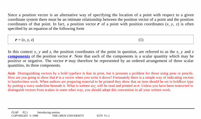
Since a position vector is an alternative way of specifying the location of a point with respect to a givencoordinate system there must be an intimate relationship between the position vector of a point and the positioncoordinates of that point. In fact, a position vector r of a point with position coordinates (x, y, z) is oftenspecified by an equation of the following form
r = (x, y, z) (1)
In this context x, y and z, the position coordinates of the point in question, are referred to as the x, y and zcomponents of the position vector r. Note that each of the components is a scalar quantity which may bepositive or negative. The vector r may therefore be represented by an ordered arrangement of three scalarquantities, its three components.
Aside Distinguishing vectors by a bold typeface is fine in print, but it presents a problem for those using pens or pencils.How are you going to show that r is a vector when you write it down? Fortunately there is a simple way of indicating vectorsin handwritten work. When authors are preparing material to be printed they show that an item should be set in boldface typeby putting a wavy underline beneath it. What is written as ~r will be read and printed as r. Unless you have been instructed todistinguish vectors from scalars in some other way, you should adopt this convention in all your written work.
FLAP P2.1 Introducing motionCOPYRIGHT © 1998 THE OPEN UNIVERSITY S570 V1.1
2.2 Displacement and distanceIt should be clear from Figure 6 that the distance from the origin of the coordinate system to the point P isnothing other than the length of the position vector r P. When dealing with vectors of any kind, includingposition vectors, it is customary to use the term magnitude when referring to their length, so we can say, quitegenerally:
The distance from the origin of a coordinate system to any particular point is given by the magnitude of theposition vector of that point.
It is worth noting that the magnitude of a vector cannot be negative. (A length may be positive or zero, but itcan’t possibly be less than zero!) Because of this it is usual to denote the magnitude of any position vector r by|1r1|, since mathematicians use a similar notation to indicate the non-negative value they call the modulus orabsolute value of any ordinary number. Of course, |1r1| is just a scalar quantity so it is also common to see itrepresented by the usual scalar symbol r. Using these notations for the magnitude of a vector we can say
r = |1r1|, the magnitude of the position vector r of a point, represents the distance from the origin of acoordinate system to that point. ☞
FLAP P2.1 Introducing motionCOPYRIGHT © 1998 THE OPEN UNIVERSITY S570 V1.1
origin
z
y
x
P
Q
rQ
sPQ
rP
Figure 73The displacement sPQ fromP to Q.
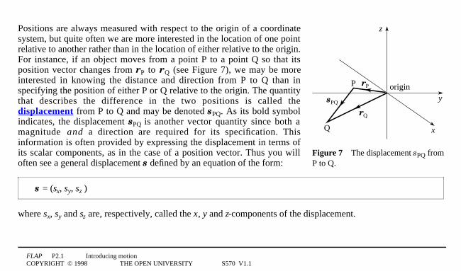
Positions are always measured with respect to the origin of a coordinatesystem, but quite often we are more interested in the location of one pointrelative to another rather than in the location of either relative to the origin.For instance, if an object moves from a point P to a point Q so that itsposition vector changes from rP to rQ (see Figure 7), we may be moreinterested in knowing the distance and direction from P to Q than inspecifying the position of either P or Q relative to the origin. The quantitythat describes the difference in the two positions is called thedisplacement from P to Q and may be denoted sPQ. As its bold symbolindicates, the displacement sPQ is another vector quantity since both amagnitude and a direction are required for its specification. Thisinformation is often provided by expressing the displacement in terms ofits scalar components, as in the case of a position vector. Thus you willoften see a general displacement s defined by an equation of the form:
s = (sx, sy, sz1)
where sx, sy and sz are, respectively, called the x, y and z-components of the displacement.
FLAP P2.1 Introducing motionCOPYRIGHT © 1998 THE OPEN UNIVERSITY S570 V1.1
We shall have more to say about the determination of these components later but for the present we shall justnote two important properties of displacement:
o Position vectors are a special class of displacements1—1they are displacements from the origin to the pointsin question.
o The magnitude of the displacement from one point to another represents the distance between those twopoints. Thus, in general:
s = |1s1|, the magnitude of the displacement from one point to another, is the distance between those twopoints.
✦ If s is the displacement from one point to another, what is wrong with the statement |1s1| = −31m?
FLAP P2.1 Introducing motionCOPYRIGHT © 1998 THE OPEN UNIVERSITY S570 V1.1
2.3 Linear motion1—1from three dimensions to oneSo far our discussion has been fully three-dimensional, just as much of physics has to be. However, in the rest ofthis module we shall be mainly concerned with linear motion1—1i.e. the motion of an object along a straightline. Although the line may point along any direction in three-dimensional space, the motion itself is really one-dimensional. If we choose to locate the origin of a coordinate system on the line and to orientate one of the axes,the x-axis say, along the line, then all the possible positions of the moving object can be specified by values ofthe single position coordinate x 1—1and that’s what characterizes one-dimensional motion. By confining ourattention to one dimension we will be able to explore some of the basic features of motion without having tomake much use of vector notation. On the other hand, because we have started from a fully three-dimensional(vector) point of view the results we obtain will be easy to generalize to three dimensions.
FLAP P2.1 Introducing motionCOPYRIGHT © 1998 THE OPEN UNIVERSITY S570 V1.1
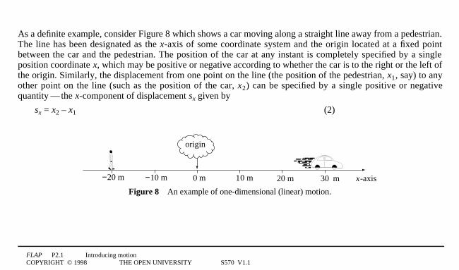
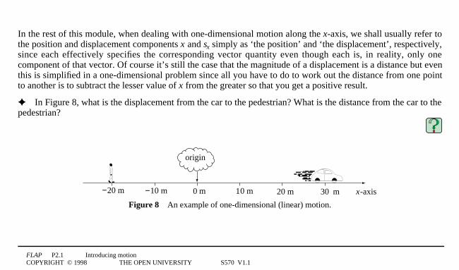
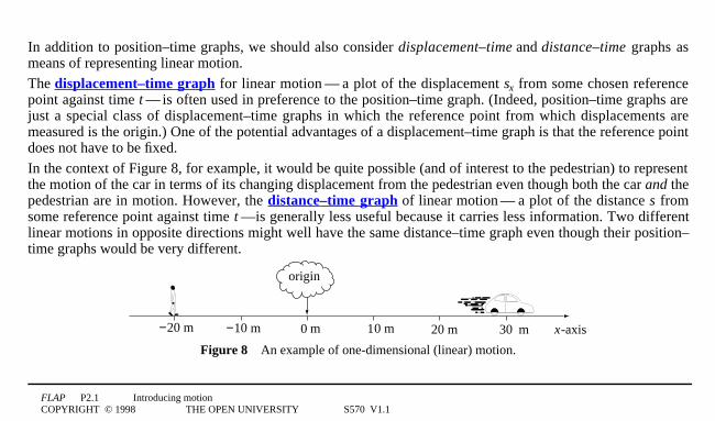
As a definite example, consider Figure 8 which shows a car moving along a straight line away from a pedestrian.The line has been designated as the x-axis of some coordinate system and the origin located at a fixed pointbetween the car and the pedestrian. The position of the car at any instant is completely specified by a singleposition coordinate x, which may be positive or negative according to whether the car is to the right or the left ofthe origin. Similarly, the displacement from one point on the line (the position of the pedestrian, x1, say) to anyother point on the line (such as the position of the car, x2) can be specified by a single positive or negativequantity1—1the x-component of displacement sx given by
sx = x2 – x1 (2)
−20 m −10 m 0 m 10 m 20 m 30 m
origin
x-axis
Figure 83An example of one-dimensional (linear) motion.
FLAP P2.1 Introducing motionCOPYRIGHT © 1998 THE OPEN UNIVERSITY S570 V1.1
In the rest of this module, when dealing with one-dimensional motion along the x-axis, we shall usually refer tothe position and displacement components x and sx simply as ‘the position’ and ‘the displacement’, respectively,since each effectively specifies the corresponding vector quantity even though each is, in reality, only onecomponent of that vector. Of course it’s still the case that the magnitude of a displacement is a distance but eventhis is simplified in a one-dimensional problem since all you have to do to work out the distance from one pointto another is to subtract the lesser value of x from the greater so that you get a positive result.
✦ In Figure 8, what is the displacement from the car to the pedestrian? What is the distance from the car to thepedestrian?
−20 m −10 m 0 m 10 m 20 m 30 m
origin
x-axis
Figure 83An example of one-dimensional (linear) motion.
FLAP P2.1 Introducing motionCOPYRIGHT © 1998 THE OPEN UNIVERSITY S570 V1.1
Table 1 The position coordinate ofthe car at various times.
Time t/s Positioncoordinate x1/m
0 0
5 1.7
10 6.8
15 15
20 26
25 39
30 53
35 68
40 84
45 99
50 115
55 131
60 146
2.4 Position–time and displacement–time graphs
To describe the motion of the car in Figure 8, we can determine its positionat various times and then display the results in a suitable way. For example,we could choose the origin of time1— 1the moment at which we start theclock and record time t2=201—1to be when the car passes the origin.We might then choose to measure the car’s position (i.e. its displacementfrom the origin) at 5-second intervals for 11minute. The results are shown inTable 1.
Note how the units are shown in such tables. The oblique slash (/) denotes aratio, thus
x/m = position coordinate in metres
1 metre(3)
so the units cancel and the entries in the table are just numbers.
These data could also be displayed visually by plotting them as points on agraph. Of course, there are conventions to bear in mind when drawing sucha graph:
FLAP P2.1 Introducing motionCOPYRIGHT © 1998 THE OPEN UNIVERSITY S570 V1.1
o Time, the independent variable, should be plotted along the horizontal axis and position, the dependentvariable, along the vertical axis. ☞
o The axes should be labelled to show what is being plotted and the label should include an oblique slash (/)followed by the appropriate units, as in the table headings.
o SI units should be used unless there are good reasons to do otherwise.
FLAP P2.1 Introducing motionCOPYRIGHT © 1998 THE OPEN UNIVERSITY S570 V1.1
Table 1 The position coordinate ofthe car at various times.
Time t/s Positioncoordinate x1/m
0 0
5 1.7
10 6.8
15 15
20 26
25 39
30 53
35 68
40 84
45 99
50 115
55 131
60 146
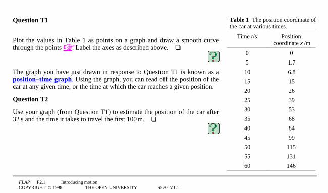
Question T1
Plot the values in Table 1 as points on a graph and draw a smooth curvethrough the points ☞. Label the axes as described above.3❏
The graph you have just drawn in response to Question T1 is known as aposition–time graph. Using the graph, you can read off the position of thecar at any given time, or the time at which the car reaches a given position.
Question T2
Use your graph (from Question T1) to estimate the position of the car after321s and the time it takes to travel the first 1001m.3❏
FLAP P2.1 Introducing motionCOPYRIGHT © 1998 THE OPEN UNIVERSITY S570 V1.1
120
100
80
60
40
20
0
− 20
10 20 30 40 50 60t/s
x/m
Figure 93The position–time graphresulting from a change of origin.
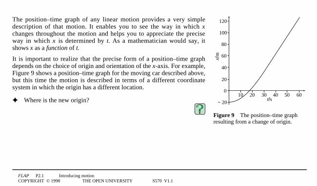
The position–time graph of any linear motion provides a very simpledescription of that motion. It enables you to see the way in which xchanges throughout the motion and helps you to appreciate the preciseway in which x is determined by t. As a mathematician would say, itshows x as a function of t.
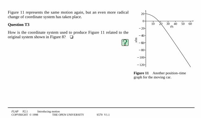
It is important to realize that the precise form of a position–time graphdepends on the choice of origin and orientation of the x-axis. For example,Figure 9 shows a position–time graph for the moving car described above,but this time the motion is described in terms of a different coordinatesystem in which the origin has a different location.
✦ Where is the new origin?
FLAP P2.1 Introducing motionCOPYRIGHT © 1998 THE OPEN UNIVERSITY S570 V1.1
20
0
− 20
− 40
− 60
− 80
− 100
− 120
10 20 30 40 50 60t/s
x/m
Figure 113Another position–timegraph for the moving car.
Figure 11 represents the same motion again, but an even more radicalchange of coordinate system has taken place.
Question T3
How is the coordinate system used to produce Figure 11 related to theoriginal system shown in Figure 8?3❏
FLAP P2.1 Introducing motionCOPYRIGHT © 1998 THE OPEN UNIVERSITY S570 V1.1
In addition to position–time graphs, we should also consider displacement–time and distance–time graphs asmeans of representing linear motion.
The displacement–time graph for linear motion1—1a plot of the displacement sx from some chosen referencepoint against time t1—1is often used in preference to the position–time graph. (Indeed, position–time graphs arejust a special class of displacement–time graphs in which the reference point from which displacements aremeasured is the origin.) One of the potential advantages of a displacement–time graph is that the reference pointdoes not have to be fixed.
In the context of Figure 8, for example, it would be quite possible (and of interest to the pedestrian) to representthe motion of the car in terms of its changing displacement from the pedestrian even though both the car and thepedestrian are in motion. However, the distance–time graph of linear motion1—1a plot of the distance s fromsome reference point against time t1—is generally less useful because it carries less information. Two differentlinear motions in opposite directions might well have the same distance–time graph even though their position–time graphs would be very different.
−20 m −10 m 0 m 10 m 20 m 30 m
origin
x-axis
Figure 83An example of one-dimensional (linear) motion.
FLAP P2.1 Introducing motionCOPYRIGHT © 1998 THE OPEN UNIVERSITY S570 V1.1
3 Velocity and speedWhen describing the three-dimensional motion of an object relative to a coordinate system we often want toknow how fast the object is travelling and in which direction. This information is given by the velocity of theobject, which is simply the rate of change of the object’s position vector with time. Since changes in positioninvolve both a direction and a magnitude it follows that velocity must also be a vector quantity that requires botha magnitude and a direction for its complete specification. For this reason velocity is usually denoted by the boldsymbol v. The magnitude of an object’s velocity is called its speed and is denoted |1v1|, though often it is simplywritten as v. Note that speed, like distance, can never be negative since it is the magnitude of a vector andmagnitudes are never negative. Indeed, you can think of speed as the rate at which distance along the path ofmotion is being covered, so it can always be described by a value, such as 301mph (or 13.31m1s–1), that can’tpossibly be less than zero. Velocity on the other hand, since it is a vector quantity and involves direction, isgenerally specified by an equation of the form
v = (vx, vy, vz1)
where the three components along the x, y and z-axes are each scalar quantities that may be positive or negative.
FLAP P2.1 Introducing motionCOPYRIGHT © 1998 THE OPEN UNIVERSITY S570 V1.1
In what follows we shall once again avoid the difficulties of dealing with velocities in their fully three-dimensional form by restricting our attention to (one-dimensional) linear motion along the x-axis of a coordinatesystem. Under such circumstances the velocity of an object is entirely specified by the x-component of itsvelocity, vx, and the speed of such an object is given by
v = |1vx1| (4) ☞
FLAP P2.1 Introducing motionCOPYRIGHT © 1998 THE OPEN UNIVERSITY S570 V1.1
30 40 50 60t/s
60
80
100
120
140
x/m
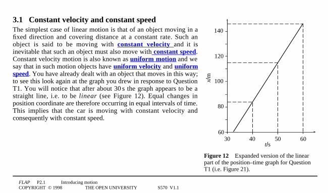
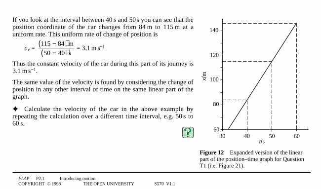
Figure 123Expanded version of the linearpart of the position–time graph for QuestionT1 (i.e. Figure 21).
3.1 Constant velocity and constant speedThe simplest case of linear motion is that of an object moving in afixed direction and covering distance at a constant rate. Such anobject is said to be moving with constant velocity and it isinevitable that such an object must also move with constant speed.Constant velocity motion is also known as uniform motion and wesay that in such motion objects have uniform velocity and uniformspeed. You have already dealt with an object that moves in this way;to see this look again at the graph you drew in response to QuestionT1. You will notice that after about 301s the graph appears to be astraight line, i.e. to be linear (see Figure 12). Equal changes inposition coordinate are therefore occurring in equal intervals of time.This implies that the car is moving with constant velocity andconsequently with constant speed.
FLAP P2.1 Introducing motionCOPYRIGHT © 1998 THE OPEN UNIVERSITY S570 V1.1
30 40 50 60t/s
60
80
100
120
140
x/m
Figure 123Expanded version of the linearpart of the position–time graph for QuestionT1 (i.e. Figure 21).
If you look at the interval between 401s and 501s you can see that theposition coordinate of the car changes from 841m to 1151m at auniform rate. This uniform rate of change of position is
vx = 115 − 84( ) m
50 − 40( ) s = 3.11m1s−1
Thus the constant velocity of the car during this part of its journey is3.11m1s−1.
The same value of the velocity is found by considering the change ofposition in any other interval of time on the same linear part of thegraph.
✦ Calculate the velocity of the car in the above example byrepeating the calculation over a different time interval, e.g. 501s to601s.
FLAP P2.1 Introducing motionCOPYRIGHT © 1998 THE OPEN UNIVERSITY S570 V1.1
✦ In what way does the velocity of 3.11m1s−1 that has just been calculated differ from a speed of 3.11m1s−1?
✦ Two cars are moving along the same line at the same speed but they have different velocities vx1 and vx2.How are the velocities related?
✦ In the case of linear motion, how can you tell by looking at a position−time graph that an object is movingat a constant velocity?
FLAP P2.1 Introducing motionCOPYRIGHT © 1998 THE OPEN UNIVERSITY S570 V1.1
t
x
t
x
t
x
t
xA B C D
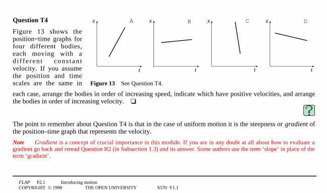
Figure 133See Question T4.
Question T4
Figure 13 shows theposition−time graphs forfour different bodies,each moving with ad i f f e r en t cons t an tvelocity. If you assumethe position and timescales are the same in
each case, arrange the bodies in order of increasing speed, indicate which have positive velocities, and arrangethe bodies in order of increasing velocity.3❏
The point to remember about Question T4 is that in the case of uniform motion it is the steepness or gradient ofthe position–time graph that represents the velocity.
Note Gradient is a concept of crucial importance in this module. If you are in any doubt at all about how to evaluate agradient go back and reread Question R2 (in Subsection 1.3) and its answer. Some authors use the term ‘slope’ in place of theterm ‘gradient’.
FLAP P2.1 Introducing motionCOPYRIGHT © 1998 THE OPEN UNIVERSITY S570 V1.1
40
30
20
10
0 10 20t/s
x/m
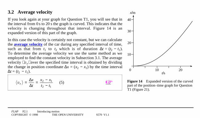
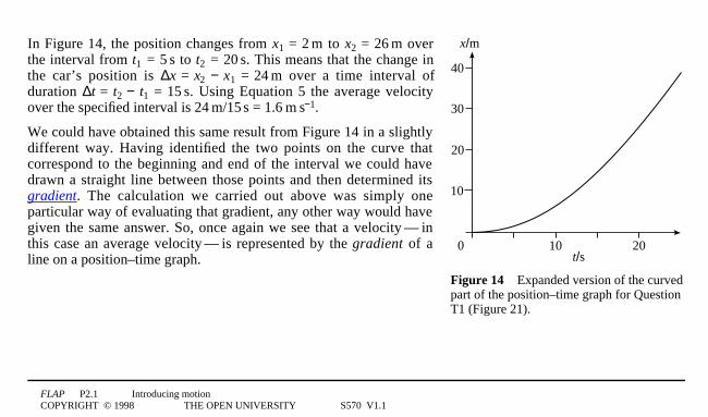
Figure 143Expanded version of the curvedpart of the position–time graph for QuestionT1 (Figure 21).
3.2 Average velocityIf you look again at your graph for Question T1, you will see that inthe interval from 01s to 201s the graph is curved. This indicates that thevelocity is changing throughout that interval. Figure 14 is anexpanded version of this part of the graph.
In this case the velocity is certainly not constant, but we can calculatethe average velocity of the car during any specified interval of time,such as that from t1 to t2 which is of duration ∆t2=2(t22−2t1).To determine the average velocity we use the same method as weemployed to find the constant velocity in Subsection 3.1. The averagevelocity ⟨ 1vx1⟩ over the specified time interval is obtained by dividingthe change in position coordinate ∆x = (x22−2x1) by the time interval∆t = (t22−2t1).
vx = ∆x
∆t= x2 − x1
t2 − t1(5) ☞
FLAP P2.1 Introducing motionCOPYRIGHT © 1998 THE OPEN UNIVERSITY S570 V1.1
40
30
20
10
0 10 20t/s
x/m
Figure 143Expanded version of the curvedpart of the position–time graph for QuestionT1 (Figure 21).
In Figure 14, the position changes from x12=221m to x22=2261m overthe interval from t12=251s to t22=2201s. This means that the change inthe car’s position is ∆x2=2x22−2x12=2241m over a time interval ofduration ∆t2=2t22−2t12=2151s. Using Equation 5 the average velocityover the specified interval is 241m/151s = 1.61m1s−1.
We could have obtained this same result from Figure 14 in a slightlydifferent way. Having identified the two points on the curve thatcorrespond to the beginning and end of the interval we could havedrawn a straight line between those points and then determined itsgradient. The calculation we carried out above was simply oneparticular way of evaluating that gradient, any other way would havegiven the same answer. So, once again we see that a velocity1—1inthis case an average velocity1—1is represented by the gradient of aline on a position–time graph.
FLAP P2.1 Introducing motionCOPYRIGHT © 1998 THE OPEN UNIVERSITY S570 V1.1
Question T5
A physics student drives at an average speed of 301mph to see a friend, who lives a distance of 601miles away(you may take the problem as being one-dimensional!). On arrival she discovers that he has misunderstood thearrangements and has already left to drive to visit her. She returns home, driving at an average speed of 601mphon the return trip. What is her average velocity for the whole journey? What is her average speed? If each leftoriginally at the same time and his average speed is 201mph, who arrives first at her house?3❏
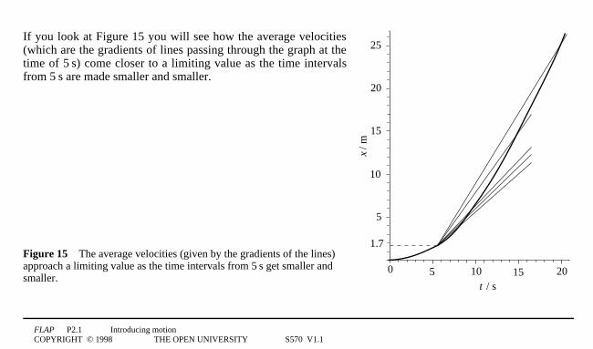
3.3 Instantaneous velocityThe average velocity we calculated in Subsection 3.2 does not give us any information about the car’s velocity atany particular instant, say at a time t2=251s. Such information is provided by another quantity called theinstantaneous velocity, which may change from moment to moment. To obtain the instantaneous velocity att2=251s we need to find the average velocity over smaller and smaller time intervals around the instant t2=251s.
Mathematically, this process of finding a better and better approximation to the car’s instantaneous velocity at apoint by shrinking the interval ∆t over which the average is taken is said to be a limiting process; we speak of
finding the limit ☞ of the average velocity as the time interval shrinks to zero.
FLAP P2.1 Introducing motionCOPYRIGHT © 1998 THE OPEN UNIVERSITY S570 V1.1
5
10
15
20
25
5 10 15 200
1.7
t / s
x / m
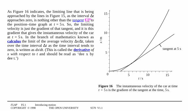
If you look at Figure 15 you will see how the average velocities(which are the gradients of lines passing through the graph at thetime of 51s) come closer to a limiting value as the time intervalsfrom 51s are made smaller and smaller.
Figure 153The average velocities (given by the gradients of the lines)approach a limiting value as the time intervals from 51s get smaller andsmaller.
FLAP P2.1 Introducing motionCOPYRIGHT © 1998 THE OPEN UNIVERSITY S570 V1.1
Mathematically, this limiting value is denoted lim∆t→0
∆x
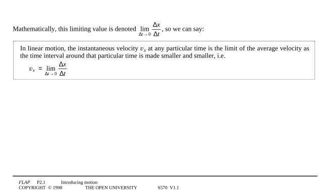
∆t, so we can say:
In linear motion, the instantaneous velocity vx at any particular time is the limit of the average velocity asthe time interval around that particular time is made smaller and smaller, i.e.
vx = lim
∆t→0
∆x
∆t
FLAP P2.1 Introducing motionCOPYRIGHT © 1998 THE OPEN UNIVERSITY S570 V1.1
5
10
15
5 10 150t / s
x / m
tangent at 5 s
Figure 163The instantaneous velocity of the car at timet2=251s is the gradient of the tangent at the time, 51s.
As Figure 16 indicates, the limiting line that is beingapproached by the lines in Figure 15, as the interval ∆tapproaches zero, is nothing other than the tangent ☞ tothe position–time graph at t2=251s. So, the limitingvelocity is just the gradient of that tangent, and it is thisgradient that gives the instantaneous velocity of the carat t2=251s. In the branch of mathematics known ascalculus the limit of the average velocity ∆x/∆t, takenover the time interval ∆t as the time interval tends tozero, is written as dx/dt. (This is called the derivative ofx with respect to t and should be read as ‘dee x bydee t.’)
FLAP P2.1 Introducing motionCOPYRIGHT © 1998 THE OPEN UNIVERSITY S570 V1.1
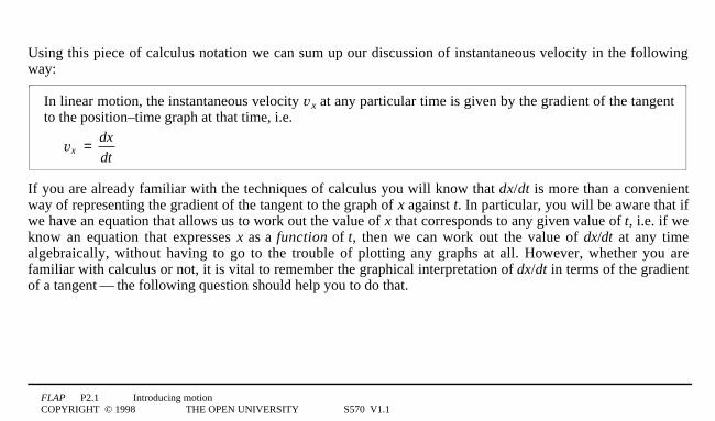
Using this piece of calculus notation we can sum up our discussion of instantaneous velocity in the followingway:
In linear motion, the instantaneous velocity vx at any particular time is given by the gradient of the tangentto the position–time graph at that time, i.e.
vx = dx
dt
If you are already familiar with the techniques of calculus you will know that dx/dt is more than a convenientway of representing the gradient of the tangent to the graph of x against t. In particular, you will be aware that ifwe have an equation that allows us to work out the value of x that corresponds to any given value of t, i.e. if weknow an equation that expresses x as a function of t, then we can work out the value of dx/dt at any timealgebraically, without having to go to the trouble of plotting any graphs at all. However, whether you arefamiliar with calculus or not, it is vital to remember the graphical interpretation of dx/dt in terms of the gradientof a tangent1—1the following question should help you to do that.
FLAP P2.1 Introducing motionCOPYRIGHT © 1998 THE OPEN UNIVERSITY S570 V1.1
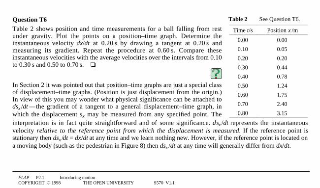
Table 233See Question T6.
Time t/s Position x1/m
0.00 0.00
0.10 0.05
0.20 0.20
0.30 0.44
0.40 0.78
0.50 1.24
0.60 1.75
0.70 2.40
0.80 3.15
Question T6Table 2 shows position and time measurements for a ball falling from restunder gravity. Plot the points on a position–time graph. Determine theinstantaneous velocity dx/dt at 0.201s by drawing a tangent at 0.201s andmeasuring its gradient. Repeat the procedure at 0.601s. Compare theseinstantaneous velocities with the average velocities over the intervals from 0.10to 0.301s and 0.50 to 0.701s.3❏
In Section 2 it was pointed out that position–time graphs are just a special classof displacement–time graphs. (Position is just displacement from the origin.)In view of this you may wonder what physical significance can be attached todsx1/dt1—1the gradient of a tangent to a general displacement–time graph, inwhich the displacement sx may be measured from any specified point. Theinterpretation is in fact quite straightforward and of some significance. dsx1/dt represents the instantaneousvelocity relative to the reference point from which the displacement is measured. If the reference point isstationary then dsx1/dt = dx/dt at any time and we learn nothing new. However, if the reference point is located ona moving body (such as the pedestrian in Figure 8) then dsx1/dt at any time will generally differ from dx/dt.
FLAP P2.1 Introducing motionCOPYRIGHT © 1998 THE OPEN UNIVERSITY S570 V1.1
In this latter case in particular it is customary to refer to dsx1/dt at any moment as the (instantaneous) relativevelocity. �☞ For example, if at some moment the pedestrian in Figure 8 has an instantaneous velocity (dx1/dt)of 11m1s–1, while that of the car (dx2/dt) is 151m1s–1, the velocity of the car relative to the pedestrian (i.e. dsx1/dt) atthat moment will be (15 – 1)1m1s–1 = 141m1s–1.
In linear motion, at any time, the instantaneous relative velocity of one body with respect to another is givenby the gradient of the tangent to the displacement–time graph, dsx1/dt, at that time, where sx is thedisplacement from the first body to the second.
All velocities are really relative velocities. Just as a position x is a special kind of displacement sx, so aninstantaneous velocity dx/dt is a special kind of instantaneous relative velocity dsx1/dt. So, if one day when outdriving you are stopped by a policeman and asked ‘how fast do you think you were travelling?’ you would bequite justified in replying ‘relative to what?’ However, you would probably be most unwise to do so.
FLAP P2.1 Introducing motionCOPYRIGHT © 1998 THE OPEN UNIVERSITY S570 V1.1
4 AccelerationThe previous section introduced a velocity that changed with time. The rate at which the velocity of a bodychanges with time is known as its acceleration. Since velocity is a vector quantity, the rate of change of velocitymust also be a vector quantity, the specification of which requires both a magnitude and a direction. In threedimensions an acceleration is therefore usually denoted by a and expressed in terms of its three (scalar)components by an equation of the form
a = (ax, ay, az1)
As usual we shall avoid dealing with this three-dimensional quantity by considering one-dimensional linearmotion in which the acceleration is entirely specified by its scalar component ax along the x-axis. The componentax may be positive or negative. A positive value for ax corresponds to an increase in vx with time and a negativevalue for ax corresponds to a decrease in vx with time. Any acceleration that causes the speed to decrease iscalled a deceleration. In the case of linear motion the magnitude of the acceleration is the positive quantitygiven by
a = |1ax1| (6) ☞
✦ What would be appropriate SI units for the measurement of a or ax?
FLAP P2.1 Introducing motionCOPYRIGHT © 1998 THE OPEN UNIVERSITY S570 V1.1
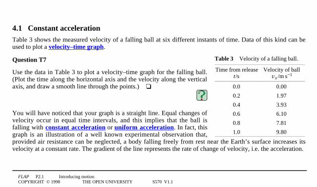
4.1 Constant accelerationTable 3 shows the measured velocity of a falling ball at six different instants of time. Data of this kind can beused to plot a velocity–time graph.
Table 33Velocity of a falling ball.
Time from releaset/s
Velocity of ballvx1/m1s−1
0.0 0.00
0.2 1.97
0.4 3.93
0.6 6.10
0.8 7.81
1.0 9.80
Question T7
Use the data in Table 3 to plot a velocity–time graph for the falling ball.(Plot the time along the horizontal axis and the velocity along the verticalaxis, and draw a smooth line through the points.)3❏
You will have noticed that your graph is a straight line. Equal changes ofvelocity occur in equal time intervals, and this implies that the ball isfalling with constant acceleration or uniform acceleration. In fact, thisgraph is an illustration of a well known experimental observation that,provided air resistance can be neglected, a body falling freely from rest near the Earth’s surface increases itsvelocity at a constant rate. The gradient of the line represents the rate of change of velocity, i.e. the acceleration.
FLAP P2.1 Introducing motionCOPYRIGHT © 1998 THE OPEN UNIVERSITY S570 V1.1
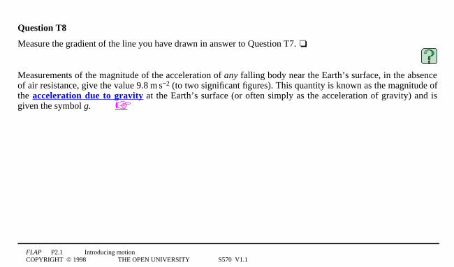
Question T8
Measure the gradient of the line you have drawn in answer to Question T7.2❏
Measurements of the magnitude of the acceleration of any falling body near the Earth’s surface, in the absenceof air resistance, give the value 9.8 1m1s−2 (to two significant figures). This quantity is known as the magnitude ofthe acceleration due to gravity at the Earth’s surface (or often simply as the acceleration of gravity) and isgiven the symbol g. ☞
FLAP P2.1 Introducing motionCOPYRIGHT © 1998 THE OPEN UNIVERSITY S570 V1.1
30
20
10
00 1 2 3 4
t/s
v /m
s−1
x
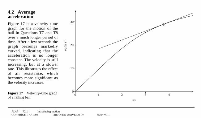
4.2 AverageaccelerationFigure 17 is a velocity–timegraph for the motion of theball in Questions T7 and T8over a much longer period oftime. After a few seconds thegraph becomes markedlycurved, indicating that theacceleration is no longerconstant. The velocity is stillincreasing, but at a slowerrate. This illustrates the effectof air resistance, whichbecomes more significant asthe velocity increases.
Figure 173Velocity–time graphof a falling ball.
FLAP P2.1 Introducing motionCOPYRIGHT © 1998 THE OPEN UNIVERSITY S570 V1.1
If we use Figure 17 we can calculate the average acceleration over a chosen period of time by means of themethod we applied to the calculation of average velocity in the previous section. This leads to the followingequation:
ax = ∆vx
∆t= vx2 − vx1
t2 − t1(7) ☞
where ∆vx2=2vx22−2vx1 is the change in vx over the interval ∆t2=2t22−2t1.
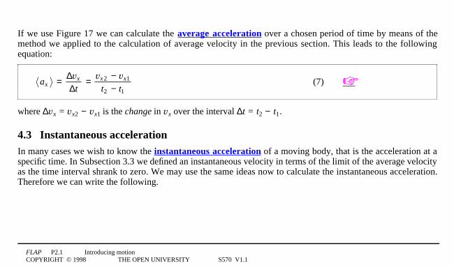
4.3 Instantaneous accelerationIn many cases we wish to know the instantaneous acceleration of a moving body, that is the acceleration at aspecific time. In Subsection 3.3 we defined an instantaneous velocity in terms of the limit of the average velocityas the time interval shrank to zero. We may use the same ideas now to calculate the instantaneous acceleration.Therefore we can write the following.

FLAP P2.1 Introducing motionCOPYRIGHT © 1998 THE OPEN UNIVERSITY S570 V1.1
In linear motion, the instantaneous acceleration ax at any particular time is the limit of the averageacceleration as the time interval around that particular time is made smaller and smaller, i.e.
ax = lim
∆t→0
∆vx
∆t
We also saw in Subsection 3.3 that calculus provides a useful shorthand for limits of this kind and that at anyparticular time such a limit may be interpreted graphically as the gradient of the tangent to an appropriate graphat that particular time. In the present case we are dealing with a velocity–time graph, so the piece of calculusnotation we need is dvx1/dt, the derivative of vx with respect to t. Using this we can say:
In linear motion, the instantaneous acceleration ax at any particular time is given by the gradient of thetangent to the velocity–time graph at that time, i.e.
ax = dvx
dt
FLAP P2.1 Introducing motionCOPYRIGHT © 1998 THE OPEN UNIVERSITY S570 V1.1
30
20
10
00 1 2 3 4
t/s
v /m
s−1
x
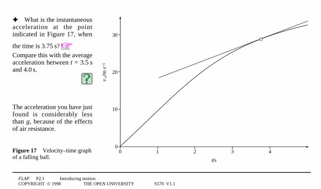
✦ What is the instantaneousacceleration at the pointindicated in Figure 17, when
the time is 3.751s? ☞Compare this with the averageacceleration between t2=23.51sand 4.01s.
The acceleration you have justfound is considerably lessthan g, because of the effectsof air resistance.
Figure 173Velocity–time graphof a falling ball.
FLAP P2.1 Introducing motionCOPYRIGHT © 1998 THE OPEN UNIVERSITY S570 V1.1
15
10
5
00 10 20 30 40 50 60
t/s
v /m
s−1
x
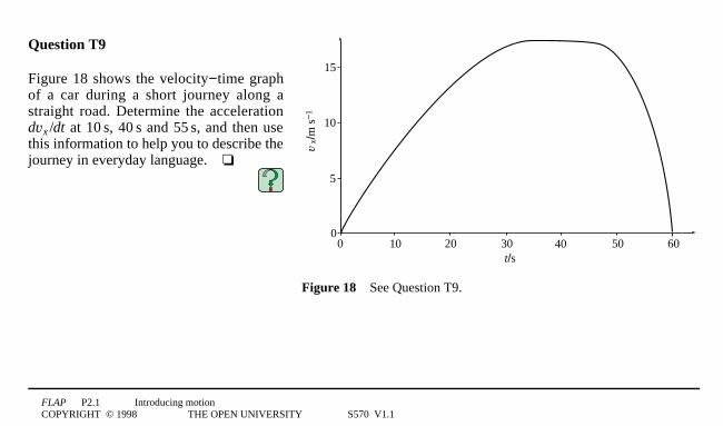
Figure 183See Question T9.
Question T9
Figure 18 shows the velocity−time graphof a car during a short journey along astraight road. Determine the accelerationdvx1/dt at 101s, 401s and 551s, and then usethis information to help you to describe thejourney in everyday language.3❏
FLAP P2.1 Introducing motionCOPYRIGHT © 1998 THE OPEN UNIVERSITY S570 V1.1
5 Equations of motionIn previous sections we have seen how the motion of an object such as a car or a ball, can be described andanalysed graphically. However, drawing graphs is time consuming and may be inaccurate, so it is highlydesirable that methods should be developed for describing and analysing motion algebraically (in terms ofequations), without the need for graphs. Such methods certainly exist and are explained in some detail in variousFLAP modules. The aim of this section is simply to introduce you to such algebraic descriptions in a way thatwill be clearly related to the graphical descriptions you have already seen. In order to keep the discussion assimple as possible we not only restrict ourselves to motion in one dimension but we further restrict ourconsiderations to moving objects that are sufficiently small and simple that they can be treated as ideal point-likeparticles. Such ideal particles have mass and occupy a definite position at any time, but unlike real objects (suchas cars or balls) they cannot rotate, bend or vibrate. Their simplicity makes them ideal subjects for ourconsiderations, and, as it turns out, an excellent starting point from which to consider more realistic objects inother modules.
We will now use the ideas developed in previous sections to derive equations that describe the motion of aparticle travelling either with constant velocity or with constant acceleration. We will not concern ourselves herewith the more general case of non-uniform acceleration.
FLAP P2.1 Introducing motionCOPYRIGHT © 1998 THE OPEN UNIVERSITY S570 V1.1
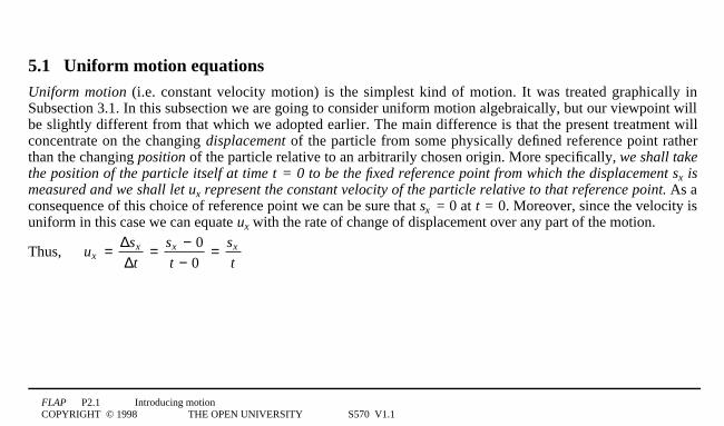
5.1 Uniform motion equationsUniform motion (i.e. constant velocity motion) is the simplest kind of motion. It was treated graphically inSubsection 3.1. In this subsection we are going to consider uniform motion algebraically, but our viewpoint willbe slightly different from that which we adopted earlier. The main difference is that the present treatment willconcentrate on the changing displacement of the particle from some physically defined reference point ratherthan the changing position of the particle relative to an arbitrarily chosen origin. More specifically, we shall takethe position of the particle itself at time t2=20 to be the fixed reference point from which the displacement sx ismeasured and we shall let ux represent the constant velocity of the particle relative to that reference point. As aconsequence of this choice of reference point we can be sure that sx 1=20 at t2=20. Moreover, since the velocity isuniform in this case we can equate ux with the rate of change of displacement over any part of the motion.
Thus, ux = ∆sx
∆t= sx − 0
t − 0= sx
t
FLAP P2.1 Introducing motionCOPYRIGHT © 1998 THE OPEN UNIVERSITY S570 V1.1
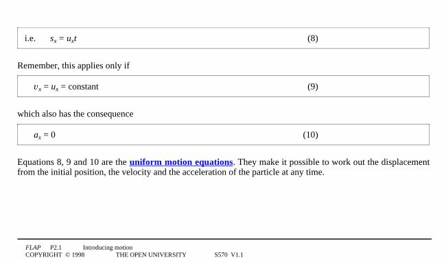
i.e. sx = uxt (8)
Remember, this applies only if
vx = ux = constant (9)
which also has the consequence
ax = 0 (10)
Equations 8, 9 and 10 are the uniform motion equations. They make it possible to work out the displacementfrom the initial position, the velocity and the acceleration of the particle at any time.
FLAP P2.1 Introducing motionCOPYRIGHT © 1998 THE OPEN UNIVERSITY S570 V1.1
ux
velo
city
time(a)
ux
velo
city
time(b)
area under the graph between t1 and t2
t1 t2
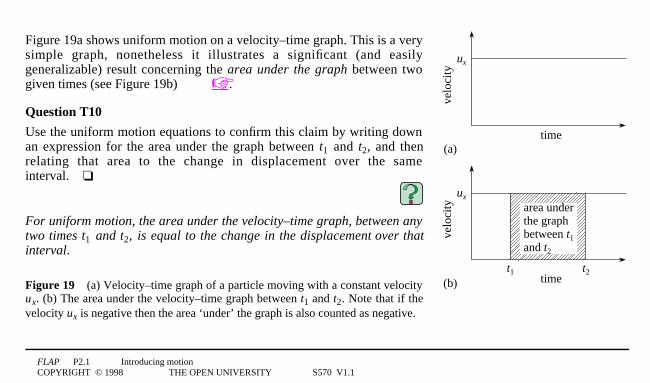
Figure 19a shows uniform motion on a velocity–time graph. This is a verysimple graph, nonetheless it illustrates a significant (and easilygeneralizable) result concerning the area under the graph between twogiven times (see Figure 19b) ☞.
Question T10
Use the uniform motion equations to confirm this claim by writing downan expression for the area under the graph between t1 and t2, and thenrelating that area to the change in displacement over the sameinterval.3❏
For uniform motion, the area under the velocity–time graph, between anytwo times t1 and t2, is equal to the change in the displacement over thatinterval.
Figure 193(a) Velocity–time graph of a particle moving with a constant velocityux. (b) The area under the velocity–time graph between t1 and t2. Note that if thevelocity ux is negative then the area ‘under’ the graph is also counted as negative.
FLAP P2.1 Introducing motionCOPYRIGHT © 1998 THE OPEN UNIVERSITY S570 V1.1
Although somewhat out of context, it is worth noting at this point that the relationship, that has just beenuncovered between the area under a velocity–time graph and the change in displacement, indicates a moregeneral result that applies even when the particle is accelerating and the area under the graph is not rectangular.
In linear motion, the area under a velocity–time graph, between two times t1 and t2, is always equal to thechange in displacement between those times.
5.2 Uniform acceleration equationsInspired by our success in dealing algebraically with uniform motion let us now move on to a slightly moredifficult case, that of a particle moving with constant or uniform acceleration. Suppose such a particle has avelocity ux at the start of its motion when t2=20, and a velocity vx at some later time t. These two velocities areknown, respectively, as the initial velocity and the final velocity. If we recall the definition of averageacceleration ⟨ 1ax1⟩ given in Equation 7, we can write the constant acceleration ax in terms of these symbols as
ax = vx − ux
t
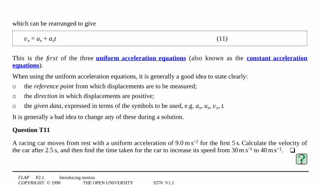
FLAP P2.1 Introducing motionCOPYRIGHT © 1998 THE OPEN UNIVERSITY S570 V1.1
which can be rearranged to give
vx = ux + axt (11)
This is the first of the three uniform acceleration equations (also known as the constant accelerationequations).
When using the uniform acceleration equations, it is generally a good idea to state clearly:
o the reference point from which displacements are to be measured;
o the direction in which displacements are positive;
o the given data, expressed in terms of the symbols to be used, e.g. ax, ux, vx, t.
It is generally a bad idea to change any of these during a solution.
Question T11
A racing car moves from rest with a uniform acceleration of 9.01m1s−2 for the first 51s. Calculate the velocity ofthe car after 2.51s, and then find the time taken for the car to increase its speed from 301m1s−1 to 401m1s−1.3❏
FLAP P2.1 Introducing motionCOPYRIGHT © 1998 THE OPEN UNIVERSITY S570 V1.1
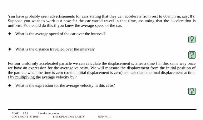
You have probably seen advertisements for cars stating that they can accelerate from rest to 601mph in, say, 81s.Suppose you want to work out how far the car would travel in that time, assuming that the acceleration isuniform. You could do this if you knew the average speed of the car.
✦ What is the average speed of the car over the interval?
✦ What is the distance travelled over the interval?
For our uniformly accelerated particle we can calculate the displacement sx after a time t in this same way oncewe have an expression for the average velocity. We will measure the displacement from the initial position ofthe particle when the time is zero (so the initial displacement is zero) and calculate the final displacement at timet by multiplying the average velocity by t.
✦ What is the expression for the average velocity in this case?
FLAP P2.1 Introducing motionCOPYRIGHT © 1998 THE OPEN UNIVERSITY S570 V1.1
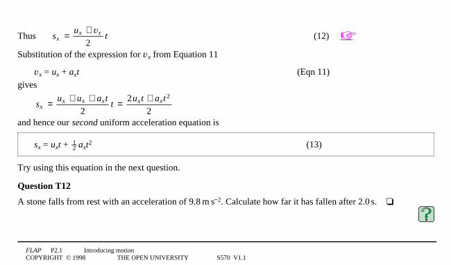
Thus sx = ux + vx
2t (12) ☞
Substitution of the expression for vx from Equation 11
vx = ux + axt (Eqn 11)
gives
sx = ux + ux + axt
2t = 2uxt + axt2
2and hence our second uniform acceleration equation is
sx = uxt + 12 axt2 (13)
Try using this equation in the next question.
Question T12
A stone falls from rest with an acceleration of 9.81m1s−2. Calculate how far it has fallen after 2.01s.3❏
FLAP P2.1 Introducing motionCOPYRIGHT © 1998 THE OPEN UNIVERSITY S570 V1.1
Aside The next question is more difficult because it requires you to use both of the uniform acceleration equations derived sofar (Equations 11 and 13), in order to eliminate the time t, which is not given in the question.
Question T13
Calculate how fast the stone in Question T12 is moving after it has fallen through 2.01m.3❏
In answering Question T13 an expression was found for the time at the end of the interval, even though thequestion did not ask for it. We could have avoided this extra effort if we had an equation which gave the finalvelocity directly in terms of the acceleration and displacement, the quantities which were given in the question.To derive such an equation we can follow the same route that was used in Question T13, but this time usealgebra to derive a general expression for the time t. We can obtain this expression by rearranging Equation 11.Thus
t = vx − ux
ax
FLAP P2.1 Introducing motionCOPYRIGHT © 1998 THE OPEN UNIVERSITY S570 V1.1
From Equation 12, the displacement is the average velocity multiplied by this time;
so sx = ux + vx
2t (Eqn 12)
and on substitution for t this gives
sx = vx
2 − ux2
2ax
This may be rearranged to give the third uniform acceleration equation
vx2 = ux
2 + 2axsx (14)
Question T14A car is travelling at an initial velocity of 6.01m1s−1. It then accelerates at 3.01m1s−2 over a distance of 201m.Calculate its final velocity.3❏
FLAP P2.1 Introducing motionCOPYRIGHT © 1998 THE OPEN UNIVERSITY S570 V1.1
Finally, it’s important to remember that all the equations derived in this subsection apply to situations in which
ax = constant (15)
Do not make the common mistake of supposing them to work in more general situations.
5.3 Solution to the introductory problemWe will return now to the problem posed in Subsection 1.1. At this point in the module you should be able tosolve this problem. Reread the problem and then consider how you would tackle it.
According to the Highway Code, a car travelling along a straight road at 301mph (i.e. about 13.31m1s−1,read as 13.31metres per second) can stop within 231metres of the point at which the driver sees a hazard.This is known as the stopping distance. If the driver always takes 0.701s to react to a hazard and applythe brakes, what is the stopping distance at 701mph (i.e. about 31.11m1s−1) assuming the samedeceleration as at 301mph?
When you have done this, have a look at the solution given below.
FLAP P2.1 Introducing motionCOPYRIGHT © 1998 THE OPEN UNIVERSITY S570 V1.1
We can divide the motion of the car into two stages. During the first stage, corresponding to the driver’s reactiontime, the car is travelling at a constant velocity. The second stage starts when the brakes are applied and we shallassume the car then has a constant deceleration. The question does not tell us the value of this constantdeceleration but since it is constant and therefore doesn’t depend on the velocity of the car we can work it outfrom the information we are given about the stopping distance of the car travelling at 30 mph (13.31m1s−1).
Within each stage of the motion, displacements will be measured from the position of the car at the beginning ofthat stage. The direction of motion will always be the positive direction for displacements, so all velocities willbe positive and deceleration will be a constant negative acceleration in this case.
For the car travelling at 13.31m1s−1, during the first stage of its motion
vx2=2ux2=2constant2=213.31m1s−1 and t2=20.701s.
To find the displacement at the end of this constant velocity stage we can use
sx = uxt (Eqn 8)
so sx = 13.31m1s−1 × 0.701s = 9.311m
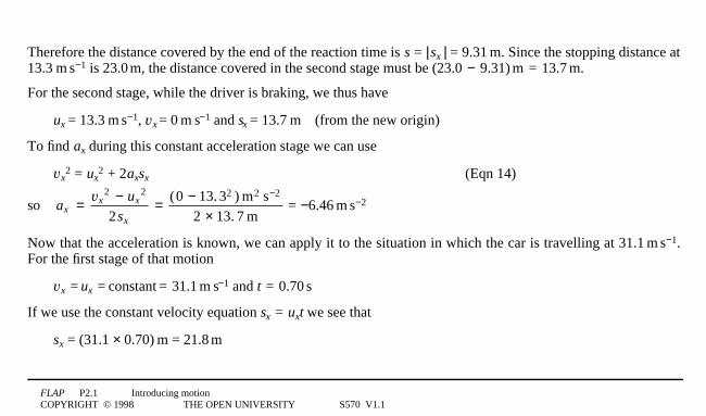
FLAP P2.1 Introducing motionCOPYRIGHT © 1998 THE OPEN UNIVERSITY S570 V1.1
Therefore the distance covered by the end of the reaction time is s = |1sx1| = 9.311m. Since the stopping distance at13.31m1s−1 is 23.01m, the distance covered in the second stage must be (23.02−29.31)1m2=213.71m.
For the second stage, while the driver is braking, we thus have
ux = 13.31m1s−1, vx = 01m1s−1 and sx = 13.71m3(from the new origin)
To find ax during this constant acceleration stage we can use
vx2 = ux
2 + 2axsx (Eqn 14)
so ax = vx
2 − ux2
2sx
= (0 − 13. 32 ) m2 s−2
2 × 13. 7 m = −6.461m1s−2
Now that the acceleration is known, we can apply it to the situation in which the car is travelling at 31.11m1s−1.For the first stage of that motion
vx2=1ux2=1constant1=231.11m1s−1 and t2=20.701s
If we use the constant velocity equation sx2=2uxt we see that
sx = (31.1 × 0.70)1m = 21.81m
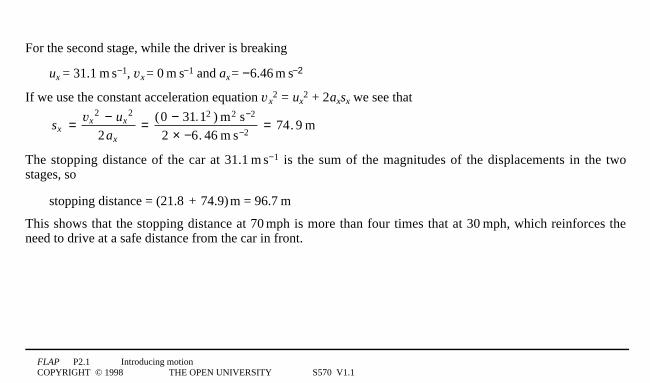
FLAP P2.1 Introducing motionCOPYRIGHT © 1998 THE OPEN UNIVERSITY S570 V1.1
For the second stage, while the driver is breaking
ux = 31.11m1s−1, vx = 01m1s−1 and ax = −6.461m1s−2
If we use the constant acceleration equation vx2 = ux
2 + 2axsx we see that
sx = vx
2 − ux2
2ax
= (0 − 31.12 ) m2 s−2
2 × −6. 46 m s−2= 74. 9 m
The stopping distance of the car at 31.11m1s−1 is the sum of the magnitudes of the displacements in the twostages, so
stopping distance = (21.82+274.9)1m = 96.71m
This shows that the stopping distance at 701mph is more than four times that at 301mph, which reinforces theneed to drive at a safe distance from the car in front.
FLAP P2.1 Introducing motionCOPYRIGHT © 1998 THE OPEN UNIVERSITY S570 V1.1
6 Closing items
6.1 Module summary1 Space is three-dimensional, so three position coordinates (x, y, z) are required to locate any point in space
relative to the origin of a Cartesian coordinate system.
2 A vector has both magnitude and direction, and may be contrasted with a scalar which has no direction.Vectors are often specified in terms of their components; these are scalar quantities that may be positive ornegative and which are measured along the axes of the coordinate system. Vector quantities include positionvector r = (x, y, z), displacement s = (sx, sy, sz1), velocity v = (vx, vy, vz1) and acceleration a = (ax, ay, az1).
3 The magnitude of a vector is the ‘length’ or ‘size’ of that vector. |1r1|, the magnitude of the position vector rof a point, represents the distance from the origin of the coordinate system to that point. Magnitudes cannever be negative.
4 The displacement s from one point to another describes the difference in their positions. |1s1| is the distancebetween those two points.
5 The velocity v of a particle is the rate of change of the position vector of that particle; it tells us how fast theparticle is moving and in what direction. |1v1| is called the speed of the particle.
6 The acceleration a of a particle is the rate of change of the velocity of that particle.
FLAP P2.1 Introducing motionCOPYRIGHT © 1998 THE OPEN UNIVERSITY S570 V1.1
7 Linear motion is motion along a straight line, though not necessarily in one direction along this line. Suchmotion is one-dimensional since the position of the moving particle can be described in terms of a singleposition coordinate, x.
8 The linear motion of a particle can be represented on a position–time graph, a displacement–time graph, ora velocity–time graph. The position–time graph shows the displacement from the origin at any time, whilethe displacement–time graph shows the displacement from some general reference point that may itself bein motion or it may be the particle’s position at t = 0.
9 If the position–time graph of a moving particle is linear, that particle must be moving with constant(uniform) velocity, i.e. with constant (uniform) speed and in a fixed direction.
10 In linear motion, the average velocity ⟨ 1vx1⟩ over a specified time interval is
vx = ∆x
∆t= x2 − x1
t2 − t1(Eqn 5)
11 In linear motion, the instantaneous velocity vx at any particular time is the limit of the average velocity asthe time interval around that particular time is made smaller and smaller. This may be written morecompactly in terms of the derivative of x with respect to t, dx/dt, which may be interpreted graphically as thegradient of the tangent to the position–time graph at the time in question. Thus,
vx = lim
∆t→0
∆x
∆t= dx
dt
FLAP P2.1 Introducing motionCOPYRIGHT © 1998 THE OPEN UNIVERSITY S570 V1.1
12 In linear motion, at any time, the instantaneous relative velocity of one body relative to another is given bythe gradient of the tangent to the displacement–time graph dsx1/dt at that time, where sx is the displacementfrom the first body to the second.
13 If the velocity–time graph of a moving particle is linear that particle must be moving with constant(uniform) acceleration.
14 In linear motion, the average acceleration ⟨ 1ax1⟩ over a specified interval is
ax = ∆vx
∆t= vx2 − vx1
t2 − t1(Eqn 7)
15 In linear motion, the instantaneous acceleration ax at a particular time is the limit of the averageacceleration as the time interval around that particular time is made smaller and smaller. This may bewritten more compactly in terms of the derivative of vx with respect to t, dvx1/dt, which may be interpretedgraphically as the gradient of the tangent to the velocity–time graph at the time in question. Thus,
ax = lim
∆t→0
∆vx
∆t= dvx
dt
FLAP P2.1 Introducing motionCOPYRIGHT © 1998 THE OPEN UNIVERSITY S570 V1.1
16 When vx = ux = constant, the uniform (linear) motion of a particle can be described algebraically using theuniform motion equations:
sx = uxt (Eqn 8)
vx = ux = constant (Eqn 9)
ax = 0 (Eqn 10)
17 When ax = constant the uniformly accelerated (linear) motion of a particle can be described algebraicallyusing the uniform acceleration equations:
vx = ux + axt (Eqn 11)
sx = uxt + 12 axt2 (Eqn 13)
vx2 = ux
2 + 2axsx (Eqn 14)
18 The area under a velocity–time graph, between two times t1 and t2 is equal to the change in displacementbetween those times.
FLAP P2.1 Introducing motionCOPYRIGHT © 1998 THE OPEN UNIVERSITY S570 V1.1
6.2 AchievementsHaving completed this module, you should be able to:A1 Define the terms that are emboldened and flagged in the margins of the module.A2 Plot position–time, displacement–time and velocity–time graphs from linear motion data.A3 Describe the linear motion of a body, given its position–time, displacement–time or velocity–time graph, or,
conversely, sketch such graphs given a description of the linear motion of the body.A4 Calculate the average velocity, or instantaneous velocity, or instantaneous relative velocity, as appropriate,
from a position–time or displacement–time graph.A5 Calculate the average acceleration, or instantaneous acceleration, as appropriate, from a velocity–time
graph.A6 Calculate the change in displacement of a particle over a given interval of time from its velocity–time graph.A7 Derive the uniform motion and constant acceleration equations and use them to solve problems.
Study comment You may now wish to take the Exit test for this module which tests these Achievements.If you prefer to study the module further before taking this test then return to the Module contents to review some of thetopics.
FLAP P2.1 Introducing motionCOPYRIGHT © 1998 THE OPEN UNIVERSITY S570 V1.1
6.3 Exit test
Study comment Having completed this module, you should be able to answer the following questions each of which testsone or more of the Achievements.
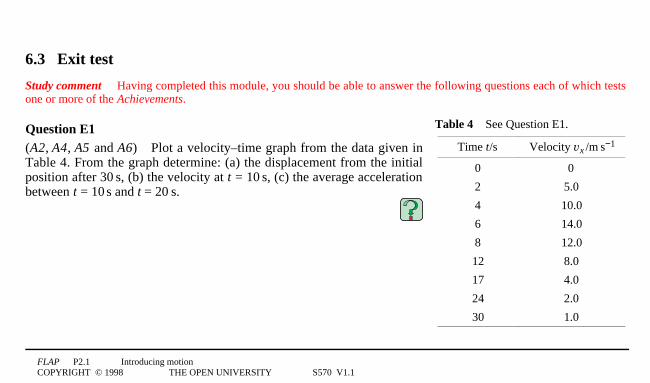
Table 43See Question E1.
Time t/s Velocity vx1/m1s−1
0 0
2 5.0
4 10.0
6 14.0
8 12.0
12 8.0
17 4.0
24 2.0
30 1.0
Question E1(A2, A4, A5 and A6)3Plot a velocity–time graph from the data given inTable 4. From the graph determine: (a) the displacement from the initialposition after 301s, (b) the velocity at t = 101s, (c) the average accelerationbetween t = 101s and t = 201s.
FLAP P2.1 Introducing motionCOPYRIGHT © 1998 THE OPEN UNIVERSITY S570 V1.1
Question E2
(A2 and A7)3A stone is released from rest and falls with uniform acceleration under gravity. Calculate itsdisplacement from its initial position over the first 31s at 0.5s intervals. For ease of calculation the magnitude ofthe acceleration due to gravity may be taken to be 101m1s−2. Use your results to plot a displacement–time graph.
If the stone were released from the top of a cliff and hit the ground at the base of the cliff 2.81s after it wasdropped, what is the height of the cliff?
FLAP P2.1 Introducing motionCOPYRIGHT © 1998 THE OPEN UNIVERSITY S570 V1.1
10
5
10 20 30t/s
0
15
20
40 50 60
v x/m
1s−
1
0
Figure 203See Question E3.
Question E3
(A3)3Write a description of the motion of a body,illustrated by the velocity–time graph in Figure 20.(You are not required to calculate displacements.)
Question E4
(A7)3(a) Derive an equation relating initial velocity,final velocity, acceleration and time for a particlemoving with a constant acceleration. (b) A lorry istravelling along a straight road at a constant velocityof 151m1s−1 when the driver notices an obstruction inthe road 251m ahead. His reaction time is 0.401s and thebrakes can produce a deceleration of 7.01m1s−2.Calculate whether the driver will stop the lorry in time.
FLAP P2.1 Introducing motionCOPYRIGHT © 1998 THE OPEN UNIVERSITY S570 V1.1
Study comment This is the final Exit test question. When you have completed the Exit test go back to Subsection 1.2 andtry the Fast track questions if you have not already done so.
If you have completed both the Fast track questions and the Exit test, then you have finished the module and may leave ithere.