möbius registration - cs.cmu.edukmcrane/projects/mobiusregistration/paper.pdf · a. baden, k....

Eurographics Symposium on Geometry Processing 2018T. Ju and A. Vaxman(Guest Editors)

Volume 37 (2018), Number 5

Möbius Registration

Alex Baden1, Keenan Crane2, and Misha Kazhdan1

1Johns Hopkins University 2Carnegie Mellon University

centeringinversion

correspondence

conformalparameterization

source

target

rotationalalignment

Figure 1: Even for near-isometric surfaces, correspondence problems can be quite challenging. Here we first compute a conformal parame-terization over the sphere (left). Since this parameterization is not unique, we must pick an inversion (center) and rotation (right) that bestregisters the two maps. We describe a fast, simple procedure for computing this transformation, and generalizations thereof.

AbstractConformal parameterizations over the sphere provide high-quality maps between genus zero surfaces, and are essential forapplications such as data transfer and comparative shape analysis. However, such maps are not unique: to define correspondencebetween two surfaces, one must find the Möbius transformation that best aligns two parameterizations—akin to picking atranslation and rotation in rigid registration problems. We describe a simple procedure that canonically centers and rotationallyaligns two spherical maps. Centering is implemented via elementary operations on triangle meshes in R3, and minimizes areadistortion. Alignment is achieved using the FFT over the group of rotations. We examine this procedure in the context of sphericalconformal parameterization, orbifold maps, non-rigid symmetry detection, and dense point-to-point surface correspondence.

Categories and Subject Descriptors (according to ACM CCS): I.3.5 [Computer Graphics]: Computational Geometry and ObjectModeling—Geometric algorithms, languages, and systems

1 IntroductionThe uniformization theorem guarantees that there is a conformalmap f : S2 → M from the sphere S2 to any genus zero surfaceM, i.e., a smooth, nondegenerate, and globally injective map thatpreserves both angles and orientation. This fact is enticing for ap-plications, since it ensures there is always a “nice” map betweenany two surfaces M1,M2 of genus zero, given by the composition

f2 ◦ f−11 of two corresponding spherical parameterizations f1, f2.

Not surprisingly, numerical algorithms for computing spherical con-formal parameterizations have received significant attention over thepast two decades [HAT∗00, GY03, GGS03, FSD05, KSS06, SSP08,KSBC12, CPS13, PKC∗16]. Unfortunately, however, for a givensurface M the parameterization f is not unique: it is determined onlyup to Möbius transformations, i.e., conformal maps from S2→ S2.

c© 2018 The Author(s)Computer Graphics Forum c© 2018 The Eurographics Association and JohnWiley & Sons Ltd. Published by John Wiley & Sons Ltd.

A. Baden, K. Crane & M. Kazhdan / Möbius Registration

Figure 2: Top: Left unchecked, iterative algorithms for sphericalconformal parameterization may apply large Möbius transforma-tions that severely distort area. Bottom right: A basic applicationof our algorithm is to prevent this “drift” by picking a canonicalinversion that centers area distortion.

Computing the best-aligned Möbius transformation is there-fore quite important, because it allows one to define a “cross-parameterization” that is determined purely by the geometry ofthe two surfaces (Figure 1), without reference to auxiliary data suchas landmark points. The resulting map can be used to transfer in-formation between two similar shapes, facilitating tasks includingsurface matching, point-to-point correspondence, detail transfer,remeshing, and shape co-analysis. For a single surface, defining acanonical Möbius inversion plays a role in, e.g., stabilizing param-eterization algorithms (Figure 2), or mitigating area distortion insurface flows [CPS13].

In this paper we propose a simple, pragmatic approach that findsa centering transformation with low area distortion via a simple iter-ative descent algorithm, then achieves rotational alignment via a fastFourier transform (FFT) over the group of rotations. For perfectlyisometric surfaces this procedure recovers an isometry; for near-isometric surfaces we get reasonably good correspondence, thoughof course quality is greatly restricted by the rigidity of Möbius trans-formations. Therefore, one way to view our method is as a fast andreliable way to initialize more challenging (e.g., nonconvex) surfaceregistration algorithms, whether conformal or not.

Outline After reviewing related work (§2) and relevant mathemat-ical background (§3), we derive a simple descent strategy that isguaranteed to produce a unique centering transformation (§4). Wethen briefly consider a generalization to non-conformal transforma-tions, providing a trade-off between angle and area distortion (§5).In §6 we give an explicit centering algorithm, and show how fastsignal processing can be used to register the rotational component.We evaluate our approach in the context of spherical conformalparameterization, spherical orbifold mapping, non-rigid symmetrydetection, and dense correspondence, highlighting some of the chal-lenges of using conformal maps for shape registration (§7). In §8we provide a summary and discussion of future work.

2 Related Work

The problem of finding the “best” Möbius transformation has beenstudied in a variety of different contexts. For some tasks (such assurface parameterization or data visualization) it is sufficient todetermine a canonical inversion; for other tasks (such as surfaceregistration) a rotation is also needed in order to align two surfaces.We consider both tasks below.

2.1 Canonical Inversion

Suppose we do not care about rotation. Which Möbius transfor-mation is canonical? Bern and Eppstein [BE01] use quasiconvexprogramming to maximize the minimum radius of a collection ofspheres or edge lengths, with applications to problems in data visu-alization and mesh generation; implementation is substantially morecomplicated than for the approach we present here, and optimizationof nonuniform triangle areas (as arise in conformal mapping) is leftas an open problem. Crane et al. [CPS13, Appendix E] considerMöbius transformations that minimize area distortion in the specialsetting of conformal surface immersions parameterized by meancurvature half density, with no guarantee of optimality.

More commonly, the canonical Möbius transformation is definedas the one that places the center of mass of a collection of pointsp1, . . . , pn at the origin. Springborn [Spr05] shows that such a trans-formation always exists and is unique; the same basic reasoningwould appear to extend to a positively-weighted sum of points orany sufficiently well-behaved mass density λ : M→ R>0.

Stereographic projection. Möbius transformations of the spherehave many different representations. One is to stereographicallymap the sphere to the plane via a point of projection p ∈ S2, apply arotation θ ∈ [0,2π), offset u ∈ R2, and positive scaling a ∈ R>0 ofthe plane, then return to the sphere via inverse stereographic projec-tion; note there are six degrees of freedom in total, corresponding tothe dimension of the Möbius group. Li & Hartley [LH07, Section4.5] directly minimize the norm of the center of mass with respectto the scaling a and offset u, which are sufficient to describe Möbiustransformations up to rotation (a statement there that the minimizercan be obtained via a linear system appears to be in error [Har18]).Koehl & Hass [KH14, Section 2.3] take the same approach to findan initial guess for subsequent a nonconvex energy (note that thisstrategy is actually different from the one of Springborn, which wediscuss below). Although the centering transformation is unique,there is no clear guarantee that gradient descent on this particularenergy will always work—for instance, the norm of the center ofmass is not a convex function of a and u, due to the inverse stereo-graphic projection. Our centering procedure (Algorithm 1) providesa simple alternative that is guaranteed to find a canonical inversion.

Homogeneous coordinates. Springborn [Spr05, Lemma 2] char-acterizes the centering Möbius transformation as the minimizerof an energy that is geodesically convex in hyperbolic space,though is not convex with respect to any coordinates on this space.To date there is very little work on geodesic convex optimiza-tion [ZS16]; a practical alternative suggested by Springborn [Spr18]is to consider Möbius transformations of the 2-sphere S2 ⊂ R3

represented as linear transformations in homogeneous coordinatesp = (x,y,z, t). In particular, let E ∈ R4×4 encode the Lorentz inner

c© 2018 The Author(s)Computer Graphics Forum c© 2018 The Eurographics Association and John Wiley & Sons Ltd.


product pTE p = x2 + y2 + z2 − t2, so that homogeneous coordi-nates satisfying pTE p = 0 correspond to points on the unit sphere.Möbius transformations are then represented by linear maps thatpreserve this inner product, and hence map the sphere to itself (theso-called Lorentz transformations). To center a collection of pointspi = (xi,yi,zi,1) on the unit sphere, one first minimizes the energyΦ(q) = ∑i log(−qTE pi/

√−qTEq) over points q = (x,y,z,1) with

(x,y,z) inside the unit ball. A Lorentz transformation is then obtainedby applying the Gram-Schmidt process (relative to E) to the vec-tors a4 = q,a1 = (1,0,0,0),a2 = (0,1,0,0),a1 = (0,0,1,0) (in thisorder), which become the columns of a matrix A = (a1,a2,a3,a4).The inverse matrix, A−1 = EATE, gives the centering inversion.Though the Hessian of Φ is not always positive-definite, one canswitch to gradient descent at indefinite points and still arrive at acanonical solution. Our strategy provides the same guarantees, but issimpler to implement and tends to converge in far fewer iterations.

Euclidean coordinates. Finally, just as every rotation of spacecan be expressed as an even number of reflections, every Möbiustransformation of the sphere can be expressed as an even number ofspherical reflections in standard Euclidean coordinates. In Section4 we consider an elementary approach to centering based on thispoint of view, yielding an iterative descent scheme (Algorithm 1)that can be directly applied to triangle meshes or point sets in R3.From a practical point of view, there appears to be no real benefitto working with stereographic projection or homogeneous coordi-nates: the simple Euclidean algorithm we describe is guaranteedto work, converges rapidly, and can be implemented via straight-forward operations in R3. Moreover, this perspective extends tocanonical spherical parameterizations that trade off between angleand area distortion (Section 5), and in principle, provides a start-ing point for defining canonical mappings on any domain (not justspheres).

2.2 Conformal Registration

To establish point-to-point correspondence between surfaces, onemust find the best-aligned Möbius transformation including rotation.Despite the importance of this problem, it has received relativelylittle attention: most earlier approaches either require landmarks(e.g., [SZS∗13,LLYG14]) or perform extensive sampling of possiblethree-point correspondences (e.g., [LF09, LPD13]). Unlike thesemethods, our approach does not require landmarks or other auxiliarydata, and does not need to perform extensive search. A notableexception is the method of Hass & Koehl [HK15], who optimize amore sophisticated (albeit nonconvex) measure of metric distortion;the resulting notion of canonical metric appears to be quite valuablefor problems in shape matching and analysis [KH14, KH15]. In thiscontext, our centering strategy can be viewed as a replacement fortheir initialization procedure. Finally, Li & Hartley [LH07] considera rotation invariant shape descriptor using spherical harmonicsrelative to a canonical Möbius inversion. This descriptor cannothowever be used to determine point-to-point correspondence.

A simple idea for performing rotational alignment is to applyprincipal component analysis to conformal scale factors, but thisapproach merely aligns quadratic terms in the Fourier expansion—ignoring the large “spikes” of area distortion typically seen in aconformal parameterization. A more sophisticated idea is to apply

Fourier-type methods directly to the Möbius group—here one en-counters two challenges. First, the group of Möbius transformationsis not compact, making it impossible to use existing generalizationsof the Fast Fourier Transform (FFT) [MR95, Roc97]. Second, theMöbius group is six-dimensional, so even if a signal-processing ap-proach were possible, the storage and run-time requirements wouldbe prohibitively expensive. From this point of view, finding a canoni-cal inversion can also be viewed as a way of reducing the dimension-ality of the problem, allowing us to facilitate a (lower-dimensional)signal processing approach to achieve alignment (Section 6).

3 ReviewWe first review some basic facts and notation that are needed toderive our basic centering algorithm.

3.1 Notation

Throughout we will use | · | and 〈·, ·〉 to denote the usual Euclideannorm and inner product on vectors in R3. For any time-varyingquantity φ(t) we will use a single dot to denote the derivative attime zero, i.e.,

φ̇ :=ddt

∣∣∣∣t=0

φ .

3.2 Möbius Transformations of the Sphere

Consider the open unit ball in R3 given by the set of points

B3 :={

x ∈ R3 : |x|< 1}.

and let S2 be the boundary of B3, i.e., the unit sphere. For any centerc ∈ B3, we can compose a spherical reflection x 7→ (x+ c)/|x+ c|2with translation and scaling to obtain a map

ηc(x) := (1−|c|2) x+ c|x+ c|2

+ c

that takes S2 to S2 (as illustrated in Figure 3). We will refer tosuch maps as inversions. All conformal maps from the sphere toitself (including rotations) can be expressed as an even number ofinversions—though for the purpose of centering (where we do notcare about rotation, and where orientation is superficial) we canconsider just a single inversion.

Figure 3: Left: An inversion ηc will push the sphere toward theinversion center c. Right: If c(t) = tu is a time-varying family ofcenters (for some fixed vector u), then the motion d

dt ηc looks like aflow toward c along the gradient of the linear function 〈u,x〉.



Figure 4: A spherical conformal parameterization f : S2→M dis-torts area by a factor λ . Viewing λ as a mass density on the sphere,we seek an inversion ηc that puts the center of mass at the origin.

4 Canonical Centering

Let f : S2→M be a spherical conformal parameterization of a genuszero surface M ⊂ R3. The area element dA on M is then related tothe standard area element dAS2 on the sphere by

dA = λdAS2 ,

where the function λ : S2→R>0 is called the conformal scale factor.We will use µ0 ∈ R3 to denote the corresponding center of mass

µ0 :=∫

S2λ (x)x dAS2 =

∫S2

x dA, (1)

i.e., the position x on the sphere, weighted by the conformal factorλ . Suppose we apply an inversion ηc to the sphere, yielding a newparameterization f ◦η−1

c with conformal factors λc. Then the newcenter of mass is

µ(c) :=∫

S2λc(x)x dAS2 =

∫S2

ηc(x) dA, (2)

since when the integral on the left is pulled back under ηc, theconformal scaling due to the η−1

c component of f ◦η−1c cancels

with the change in area due to the pullback. We seek an inversionthat moves the center of mass to the origin (i.e., µ(c) = 0), whichcan be acheived by minimizing the energy

E := 12 |µ(c)|

2

with respect to the inversion center c. (Note that we do not need toconsider rotations, which have no effect on the norm.) The corre-sponding gradient is given by

∇cE = JTµ µ, (3)

where Jµ denotes the Jacobian of µ with respect to c (and T denotesthe transpose). To compute this Jacobian, consider a time-varyinginversion center c(t) := tu for some fixed vector u ∈ R3. The timederivative of ηc at t = 0 is then

12 η̇c(t)(x) = u−〈u,x〉x.

In other words, moving the center of inversion toward u causes eachpoint x to slide tangentially on the sphere, along the direction closestto u. As a result, the sphere will gradually contract near the head ofu, and expand near its tail (consider Figure 3, right). Applying our

expression for η̇ to Equation 2, we then get

µ̇ = 2∫

S2u−〈u,x〉x dA.

Noting that Jµ u = µ̇ for all u, the Jacobian at c = 0 is therefore

Jµ

∣∣c=0 = 2

∫S2

id− x⊗ x dA, (4)

where id denotes the identity, and ⊗ is the outer-product.

4.1 Existence and Uniqueness

Following the gradient ∇cE will always yield a unique center c∈ B3

that places the center of mass µ at the origin. To see why, firstnote that the Jacobian Jµ has full rank, since it is a positive linearcombination of linearly independent rank-2 operators id− x⊗ x.Hence, the energy gradient ∇cE = JTµ µ will be zero if and only ifµ0 = 0, i.e., if the center of mass is already at the origin. Moreover,as the center approaches the boundary of the ball, the energy tendstoward its maximum value, i.e., lim|c|→1 E = c

∫S2 dA. Hence, there

must be a minimum at some point on the interior of B3. To see thatthe centering inversion is unique, recall that an inversion moveseach point toward the centering direction c (except for the poles±c).Hence,

〈c,ηc(x)〉 ≥ 〈c,x〉.

Suppose the center of mass is already at the origin, i.e., µ0 = 0, andlet µ(c) be the center obtained by applying an inversion with anycenter c ∈ B3. Then

〈c,µ(c)〉=∫

S2〈c,ηc〉 dA >

∫S2〈c,x〉 dA = 〈c,µ0〉= 0.

(Note that the inequality is strict since λ is a smooth function; hence,not all mass can be concentrated at the poles.) Hence, there can beno inversion that leaves the center of mass at the origin.

5 Generalized Centering

In Section 4 we studied the centering problem via explicit geomet-ric calculations in R3. In this section we consider an alternative,functional perspective that naturally generalizes beyond conformaltransformations of the sphere. To make a link between the two pointsof view, suppose that x= (x1,x2,x3) are coordinates on R3. Then wecan think of µ as the projection of the conformal factor λ onto thespace of linear functions spanned by the corresponding coordinatefunctions ei : S2→R;x 7→ xi. In other words, we can identify µ withthe function 3

4π ∑3i=1(

∫S2 λ ei dAS2)ei. Additionally, infinitesimal

inversions look like gradients of linear functions, i.e., for c(t) = tu,we have

12 η̇c(t)(x) = u−〈u,x〉x = ∇〈x,u〉,

as depicted in 3, right. Hence, the center of mass µ is zero if and onlyif the conformal factors vanish when projected onto the space oflinear functions; if µ is nonzero, then we can always reduce its normby “flowing” along the gradient of some linear function. Ratherthan thinking about conformal factors, we could also just say: theparameterization is centered if the coordinate functions on S2 vanishwhen integrated with respect to the area of the target surface. As wewill see in Section 5.2, the notion of a centered parameterization can



therefore be generalized by replacing the linear functions with anycollection of smooth functions F , and the area element dA with avolume form ω on any manifold. Likewise, our centering motionswill no longer be infinitesimal Möbius transformations, but ratherflows along gradients of functions in F . The key observation isthat, as with the sphere, a parameterization that is not centered canalways be improved by such motions, i.e., the norm of the center µ

has local minima only when µ = 0.

5.1 Preliminaries

We briefly review some basic concepts needed for our generaliza-tion; more detailed discussion can be found in a standard text ondifferentiable manifolds, such as Abraham et al. [AMR93]. Let Mbe a compact connected orientable n-manifold without boundary,and let dV be the volume form on M—in the context of Section 4,for instance, M = S2 and dV = dAS2 . We will use ‖ · ‖ and 〈〈·, ·〉〉 todenote the L2 norm and inner product (resp.) with respect to dV .

A smooth vector field X on M defines a flow map FX ,t : M→Mobtained by following integral curves of X for time t; this map isalways well-defined and invertible up to some sufficiently smalltime T > 0. We will use (FX ,t)∗ω to denote the pushforward of ann-form ω under such a flow. The Lie derivative

LX ω := ddt

∣∣∣t=0

(F−X ,t)∗ω (5)

then describes the infinitesimal change in ω as we advect it along−X . For any scalar function φ , the Lie derivative satisfies a productrule LX (φω) = φLX ω +(LX φ)ω , and for an n-form on a manifoldwithout boundary we have

∫M LX (φω) = 0 (by Cartan’s formula

and Stokes’ theorem). Hence,∫M

φLX ω =−∫

M(LX φ)ω, (6)

i.e., under a flow along X , integration of a function φ simplychanges by (minus) the directional derivative of f along X . Forscalar functions, the Lie derivative is just the directional derivative,i.e., LX φ = 〈X ,∇φ〉, where ∇φ is the gradient of φ .

5.2 Generalized Centering

Consider a k-dimensional space of functions F ⊂W 1,2(M), none ofwhich are constant. We define the center of mass of a volume formω relative to F as the unique function µ0(ω) ∈ F satisfying

〈〈ψ,µ0(ω)〉〉=∫

Mψω (7)

for all ψ ∈F . Equivalently, if F has an orthonormal basis e1, . . . ,ek,then µ0(ω) = ∑

ki=1 (

∫M ekω)ek, i.e., µ0(ω) is effectively the “pro-

jection” of ω onto F . For any function φ ∈ F , we then define

µ(φ) := µ0((F∇φ ,1)∗ω)

as the center of mass obtained by flowing the volume form ω alongthe gradient of φ . We say that φ centers ω (with respect to F ) whenµ(φ) = 0, and can measure how far we are from being centered viathe energy

E := 12‖µ‖

2.

We then get a result that generalizes the one we had for inversions:

Theorem: If µ(φ) 6= 0, then there is a function ψ ∈ F such thatflowing ω along the gradient vector field X = ∇ψ reduces the quan-tity ‖µ‖2, i.e., we can always bring µ(φ) closer to the origin.

Proof: We proceed essentially as in Section 4: the gradient of theenergy E can be expressed as ∇φ E = JTµ µ , where Jµ : F → Fdenotes the Jacobian of µ with respect to φ . To evaluate Jµ ψ atφ = 0, consider a time-varying function ϕ(t) = tψ for any fixedfunction ψ ∈ F . Then

Jµ ψ∣∣φ=0 =

ddt

∣∣∣t=0

µ(ϕ(t)) = ddt

∣∣∣t=0

µ0((F∇ψ,t)∗ω).

Taking the L2 inner product with ψ and applying Equation 7 gives

〈〈ψ,Jµ ψ〉〉∣∣φ=0 =

∫M

ψddt

∣∣∣t=0

(F∇ψ,t)∗ω,

and applying Equations 5 and 6 then yields

〈〈ψ,Jµ ψ〉〉∣∣φ=0 =

∫M

ψL−∇ψ ω =∫

M(L∇ψ ψ)ω =

∫M〈∇ψ,∇ψ〉ω.

Since F contains no constant functions, ∇ψ must be nonzero; more-over, ω is a volume form and hence positive everywhere. As in thecase of inversions, then, the Jacobian Jµ is strictly positive definite,and hence the energy gradient ∇E will vanish at φ = 0 if and onlyif µ0(ω) is zero, i.e., if ω is centered. �

Uniqueness of the centering motion is less clear—the argumentused for Möbius transformations of the sphere was purely geometric,and hence does not generalize to the functional setting. Note thatin practice, Jµ is just a real k× k matrix which can be used toimplement a descent algorithm that looks identical to Algorithm 1;here the function φ plays the role of the center c, and inversion isreplaced by advection along ∇φ .

Example: Higher-Order Harmonics

A trivial example of centering in this framework would be to letF be the linear functions on M = Rn; in this case our procedureflows mass along the corresponding constant vector fields, whichis the same as just translating the center of mass to the origin. Asa more interesting example we return to the case of the sphere,

input degree 1 degree 1, 2 degree 1, 2, 3

Figure 5: By considering centering motions beyond just Möbiustransformations, we can trade off between area and angle distortion.Here we use gradients of spherical harmonics of increasing degree.



and seek a parameterization that is centered with respect to somecollection of “low-frequency” functions—in particular, we let Fconsist of low-order spherical harmonics, as shown in Figure 5. Fordegree-one harmonics (just linear functions) we get only infinites-imal inversions; for progressively higher order harmonics we getadditional, non-conformal motions that allow better distribution ofarea, at the cost of angle distortion. This picture also makes it clearthat our Möbius centering procedure eliminates any “low-frequency”area distortion, since the linear component of the conformal scalefactors λ vanishes. Here and in similar experiments we find that ourprocedure always yields a centered parameterization (µ(ω) = 0).

Non-Gradient Flows

In addition to transformations characterized by flows along gradientsof functions, one would also like to consider transformations alongdivergence-free vector fields. Unfortunately, our centering approachdoes not extend to these cases and we believe that centering withrespect to divergence-free transformations is much harder. In thecase of the sphere, for example, inversions are characterized bythe gradients of linear functions. Applying a pointwise 90-degreerotation, we obtain the complimentary space of divergence-freevector fields. These characterize (infinitesimal) rotations, completingthe group of Möbius transformations. As we cannot center withrespect to them, the next section describes and efficient approachfor aligning over the space of rotations.

6 Möbius Registration

We now consider the task of finding correspondence between twogenus zero surfaces, which we perform in three steps: first computea conformal parameterization of each surface over the sphere, usingany method (see references in Section 1), find canonical centeringinversions (Section 6.1), and finally compute the rotation that bestaligns the two centered parameterizations (Section 6.2). Though ourmethod can in principle be applied to any surface representation,we give an explicit algorithm for triangle meshes. We will assumethat each input mesh is encoded by a collection of triangles T withareas A :→ R>0 from the original surface M, and will assume thatthe vertices V ⊂ S2 have already been mapped to the unit sphereS2. (To instead apply our algorithm to a set of points P ⊂ S2, onecan simply replace the triangle centers with P and the triangle areaswith A ≡ 1 in Algorithm 1.) A complete implementation of thisprocedure, including spherical parameterization, can be found athttps://github.com/mkazhdan/MoebiusRegistration.

6.1 Centering Algorithm

The analysis in Section 4 suggests a simple algorithm for centeringa given parameterization: simply perform gradient descent on theenergy E with respect to the inversion center c, starting at any pointin B3. Since the gradient vanishes only at the global minimum (andthe energy goes to 1

2 (∫

S2 ω)2 as c approaches the boundary of B3),we will always obtain a canonical centering, up to rotation. Sincewe have an explicit expression for the Jacobian Jµ of the center withrespect to c, this algorithm can easily be accelerated using Gauss-Newton iterations rather than simple gradient iterations, as shownin Algorithm 1. Here, C(τ) denotes the center of mass of a triangle

Algorithm 1 MÖBIUSCENTER(T,V,A,ε)Input: A mesh with triangles T , areas A : T → R>0, a conformal

parameterization specified by vertex coordinates V ⊂ S2, and astopping tolerance ε > 0. (C(τ) denotes the center of τ , normal-ized to have unit length.)

Output: Centered vertex coordinates V ⊂ S2.1: while true2: µ ← ∑τ∈T C(τ)A(τ) . compute center of mass3: if |µ| ≤ ε then break4: Jµ ← 2∑τ∈T A(τ)(I−C(τ)C(τ)T) . build Jacobian5: c←−J−1

µ µ . compute inversion center6: for v ∈V7: v← (1−|c|2) v+c

|v+c|2 + c . apply inversion

8: return V

τ; for simplicity we use the average of its vertices. We do not needto explicitly compute the conformal scale factors λ , since they arealready accounted for by the area weights A. The simple form of theGauss-Newton update arises from the fact that Jµ is symmetric, andhence −(JTµ Jµ )

−1JTµ =−J−1µ . Here we use a unit time step, though

for larger or more challenging models it may be helpful to take asmaller step (i.e., replace c with αc for some constant α ∈ (0,1))or perform an explicit line search (setting the energy of centers coutside the unit ball to infinity). Note that this algorithm assumesthat vertices v are on the unit sphere, i.e., |v|2 = 1; it will not workproperly for spheres of other radii.

Generalized centering. To center with respect to a general col-lection of functions F with orthonormal basis e1, . . . ,ek, we maketwo modifications to Algorithm 1. First, C(τ) returns a vector con-taining the value of each basis function at the triangle center. Second,the transformation in Line 7 is replaced by numerical advection ofthe spherical triangulation along the gradient of c, which is nowviewed as a function on M. That is, we move each vertex along thesurface M with velocity determined by the gradient. Here one mustbe careful to take sufficiently small time steps, in order to avoidtriangle flips.

6.2 Rotational Alignment

We next seek the rotation that best aligns the two parameterizations.To do so, we first sample the conformal factors of each mesh onto aregular spherical grid (Figure 6, top right). We then find the rotationthat maximizes the correlation between conformal factors, via a fastspectral transform.

Sampling conformal factors. Given a centered mesh (V,T ) withoriginal areas A : V → R>0, we compute the total area containedin each cell of a regular spherical grid, divided by the area of thespherical cell—these values represent the average conformal factorover the cell (Figure 6, bottom right). Note that simply samplingthe area ratio at the cell center can yield significant aliasing, sincea conformal parameterization may map a large region of the meshto a very small region on the sphere. We likewise apply a low-passfilter to further reduce potential aliasing (Figure 6, bottom left).


https://github.com/mkazhdan/MoebiusRegistration


max0|λ|

input tessellated

scalefactors

scale factors(low-pass)

Figure 6: Prior to rotational alignment, the input mesh (top left)is parameterized, centered, and tessellated by an equirectangulargrid (top right). Sampled conformal factors (bottom right) are thenlow-pass filtered (bottom left) to mitigate aliasing. (Scale factorsare visualized by scaling points on the unit sphere according to |λ |.)

Aligning conformal factors. To obtain our final registration, wecompute the rotation that maximizes the correlation between thescale factors sampled from the two meshes. This rotation is obtainedin three steps: (1) We compute the forward fast spherical harmonictransform [HRKM03] to get an expression of each spherical func-tion in terms of the spherical harmonics. (2) We cross-multiply thespherical harmonic coefficients within each frequency band to obtainthe coefficients of the correlation in terms of the rotational harmon-ics. (3) We apply the fast inverse Wigner-D transform [KR08] toobtain a sampling of the correlation on a regular 3D grid of Eulerangles. Since the input functions are band-limited, the correlationfunction is also band-limited; to robustly detect maxima we use aregular grid whose resolution is twice the band-width. To get anorientation-reversing registration (e.g., for reflective symmetry de-tection), we can simply apply a reflection to one of the two sampledfunctions. Note that if either shape has rotational symmetries wewill of course obtain only one possible registration; this ambiguity isa fundamental feature of the registration problem (and has nothingto do with our particular algorithm).

7 EvaluationTo evaluate our approach we consider four applications: stabiliz-ing a spherical conformal parameterization algorithm, computingspherical orbifold parameterizations, detecting non-rigid intrinsicsymmetry, and finding dense point-to-point correspondence. Thefirst two examples demonstrate the utility of our approach; the lattertwo illustrate some of the challenges faced when using conformalparameterization for surface registration. We also provide somebasic information about performance.

7.1 Stabilizing Conformal Parameterization

In principle, one might expect algorithms for spherical conformalparameterization to be oblivious to Möbius transformations, but inreality discretization error causes certain Möbius transformationsto be preferred. For instance, one way to obtain a conformal map isto minimize Dirichlet energy, which for the sphere is naturally dis-cretized as 1

4 ∑e weθ 2e , where θe is the angle between the endpoints

of an edge e (i.e., an arc on the sphere S2), and we is the correspond-ing cotangent weight (from the input domain M). A trivial way tominimize this energy is to move all vertices to a common point,and this is exactly the kind of behavior observed in many iterativealgorithms: the parameterization “drifts” toward a Möbius transfor-mation that concentrates all vertices at a point. We can prevent thisbehavior by simply applying our centering algorithm (Algorithm 1),as demonstrated in Figure 2 for a conformal map computed viaconformalized mean curvature flow (CMCF) [KSBC12].

7.2 Spherical Orbifold Parameterization

A spherical orbifold is a quotient of the sphere S2 by a finite groupof rotations—intuitively, a tiling of the sphere. Conformal parame-terization over such domains has recently been explored as a wayto reduce area distortion for genus zero surfaces [AKL17]. We con-sider a different algorithmic approach: first, we create a multiplecovering M̃ of the input geometry M, then we compute a conformalparameterization of this covering over the sphere. By centering this

inputuncentered centered

Figure 7: Spherical orbifold maps with cyclic symmetry (top) andtetrahedral symmetry (bottom). Though an arbitrary spherical con-formal parameterization of a covering space might not be rotation-ally symmetric (center), our centering procedure ensures that itexhibits the desired orbifold symmetry (right). Black lines indicatecuts made on the input mesh (left).



distance0.40%

50%

100%

0.5 0.6 0.7

centeredcentered

uncentereduncentered

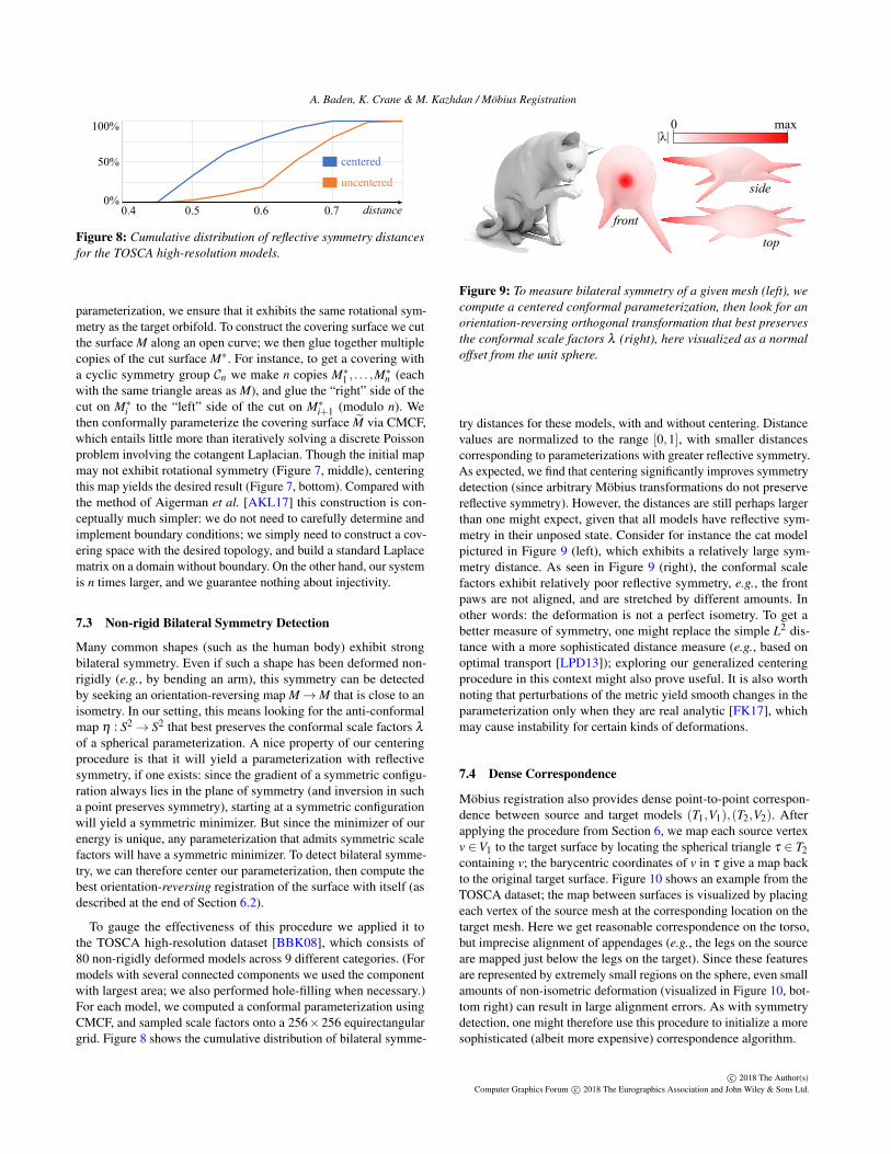
Figure 8: Cumulative distribution of reflective symmetry distancesfor the TOSCA high-resolution models.

parameterization, we ensure that it exhibits the same rotational sym-metry as the target orbifold. To construct the covering surface we cutthe surface M along an open curve; we then glue together multiplecopies of the cut surface M∗. For instance, to get a covering witha cyclic symmetry group Cn we make n copies M∗1 , . . . ,M

∗n (each

with the same triangle areas as M), and glue the “right” side of thecut on M∗i to the “left” side of the cut on M∗i+1 (modulo n). Wethen conformally parameterize the covering surface M̃ via CMCF,which entails little more than iteratively solving a discrete Poissonproblem involving the cotangent Laplacian. Though the initial mapmay not exhibit rotational symmetry (Figure 7, middle), centeringthis map yields the desired result (Figure 7, bottom). Compared withthe method of Aigerman et al. [AKL17] this construction is con-ceptually much simpler: we do not need to carefully determine andimplement boundary conditions; we simply need to construct a cov-ering space with the desired topology, and build a standard Laplacematrix on a domain without boundary. On the other hand, our systemis n times larger, and we guarantee nothing about injectivity.

7.3 Non-rigid Bilateral Symmetry Detection

Many common shapes (such as the human body) exhibit strongbilateral symmetry. Even if such a shape has been deformed non-rigidly (e.g., by bending an arm), this symmetry can be detectedby seeking an orientation-reversing map M→M that is close to anisometry. In our setting, this means looking for the anti-conformalmap η : S2→ S2 that best preserves the conformal scale factors λ

of a spherical parameterization. A nice property of our centeringprocedure is that it will yield a parameterization with reflectivesymmetry, if one exists: since the gradient of a symmetric configu-ration always lies in the plane of symmetry (and inversion in sucha point preserves symmetry), starting at a symmetric configurationwill yield a symmetric minimizer. But since the minimizer of ourenergy is unique, any parameterization that admits symmetric scalefactors will have a symmetric minimizer. To detect bilateral symme-try, we can therefore center our parameterization, then compute thebest orientation-reversing registration of the surface with itself (asdescribed at the end of Section 6.2).

To gauge the effectiveness of this procedure we applied it tothe TOSCA high-resolution dataset [BBK08], which consists of80 non-rigidly deformed models across 9 different categories. (Formodels with several connected components we used the componentwith largest area; we also performed hole-filling when necessary.)For each model, we computed a conformal parameterization usingCMCF, and sampled scale factors onto a 256×256 equirectangulargrid. Figure 8 shows the cumulative distribution of bilateral symme-

max0|λ|

front

side

top

Figure 9: To measure bilateral symmetry of a given mesh (left), wecompute a centered conformal parameterization, then look for anorientation-reversing orthogonal transformation that best preservesthe conformal scale factors λ (right), here visualized as a normaloffset from the unit sphere.

try distances for these models, with and without centering. Distancevalues are normalized to the range [0,1], with smaller distancescorresponding to parameterizations with greater reflective symmetry.As expected, we find that centering significantly improves symmetrydetection (since arbitrary Möbius transformations do not preservereflective symmetry). However, the distances are still perhaps largerthan one might expect, given that all models have reflective sym-metry in their unposed state. Consider for instance the cat modelpictured in Figure 9 (left), which exhibits a relatively large sym-metry distance. As seen in Figure 9 (right), the conformal scalefactors exhibit relatively poor reflective symmetry, e.g., the frontpaws are not aligned, and are stretched by different amounts. Inother words: the deformation is not a perfect isometry. To get abetter measure of symmetry, one might replace the simple L2 dis-tance with a more sophisticated distance measure (e.g., based onoptimal transport [LPD13]); exploring our generalized centeringprocedure in this context might also prove useful. It is also worthnoting that perturbations of the metric yield smooth changes in theparameterization only when they are real analytic [FK17], whichmay cause instability for certain kinds of deformations.

7.4 Dense Correspondence

Möbius registration also provides dense point-to-point correspon-dence between source and target models (T1,V1),(T2,V2). Afterapplying the procedure from Section 6, we map each source vertexv ∈V1 to the target surface by locating the spherical triangle τ ∈ T2containing v; the barycentric coordinates of v in τ give a map backto the original target surface. Figure 10 shows an example from theTOSCA dataset; the map between surfaces is visualized by placingeach vertex of the source mesh at the corresponding location on thetarget mesh. Here we get reasonable correspondence on the torso,but imprecise alignment of appendages (e.g., the legs on the sourceare mapped just below the legs on the target). Since these featuresare represented by extremely small regions on the sphere, even smallamounts of non-isometric deformation (visualized in Figure 10, bot-tom right) can result in large alignment errors. As with symmetrydetection, one might therefore use this procedure to initialize a moresophisticated (albeit more expensive) correspondence algorithm.



source target

anisotropic distortionsource target

Figure 10: Dense correspondence between source and target mod-els (top) is visualized by placing each vertex of the source mesh atthe corresponding location on the target mesh (bottom left). Non-isometric deformation (bottom right) can cause substantial misalign-ment of features that are mapped to small regions on the sphere(anisotropy σ is the ratio of larger to smaller singular value).

model vertices center tessellate correlateoctopus 10K 0.01 0.2 / 0.4 / 1.3 0.3 / 2.2 / 27centaur 16K 0.02 0.2 / 0.4 / 1.2 0.2 / 2.1 / 27cat 28K 0.02 0.3 / 0.6 / 1.5 0.3 / 2.2 / 30Michael 53K 0.06 0.3 / 0.6 / 1.4 0.3 / 2.2 / 28hand 66K 0.09 0.7 / 1.1 / 2.7 0.3 / 2.2 / 28bunny 104K 0.09 0.9 / 1.6 / 3.5 0.3 / 2.2 / 28armadillo 173K 0.17 1.0 / 1.6 / 3.3 0.3 / 2.2 / 27

Table 1: Timings for the different stages of processing. For tessella-tion and correlation we use equirectangular grids of resolution N =128, 256, and 512. All times are in seconds.

7.5 Performance

Table 1 gives timings for Möbius centering, spherical tessellation,and correlation, for several models and at several different gridresolutions. Timings were measured on a Windows PC with anIntel Core i7-6600 processor and 16 GB of RAM. The centeringprocedure appears to have linear complexity, typically achieving acenter norm of about 10−10 in three or four iterations. Tessellation isless efficient, but still linear in the number of vertices (absolute costdepends on the number of grid cells containing each triangle). Thecost of computing the final rotational correlation is independent ofmesh complexity; for an N×N grid, the inverse Fourier transformover the rotation group has a cost in O(N4).

8 ConclusionThe allure of uniformization is that it provides a near-canonical mapbetween surfaces of equivalent topology, but as we have seen, work-ing purely in the conformal setting can be quite restrictive whenit comes to applications. Other, more flexible notions of canoni-cal mappings have the potential to be quite powerful in geometryprocessing—though many questions remain to be explored. Ideally,one would like to find maps that are not only canonical, but alsoexhibit low metric distortion (i.e., small distortion of both anglesand areas). Replacing the geometric picture of Möbius transforma-tions with the more functional picture introduced in Section 5 yieldsan enticing framework for this problem, with many questions thatremain to be explored. For instance, we know very little about theconditions under which the generalized center exists and is unique;we also have no strategy for centering with respect to nonintegrablemotions (i.e., vector fields that do not arise from a scalar potential).It is also natural to consider more informative notions of distancebeyond L2 (e.g., the Wasserstein distance), or centering with respectto other conformally invariant 2-forms (e.g., the square-norm ofthe gradient of the heat-kernel-signature). Finally, there is the ques-tion of how different choices of centering motions (i.e., differentchoices of the space F ) impact geometric properties of the centeredparameterization. For instance, one can always use the Laplacianeigenfunctions to get a space of low-frequency deformations, but itis not clear that these motions are ideal for, e.g., minimizing metricdistortion. Overall, we are hopeful that the functional, flow-basedpoint of view will spark new ideas about how to define and constructcanonical maps between surfaces, just as it has provided a valuableperspective on canonical Möbius transformations of the sphere.

AcknowledgementsThanks to Boris Springborn and Richard Hartley for discussionsabout their algorithms, and Northside Social for providing collabo-rative work space. Thanks to Patrice Koehl for feedback on practicalimplementation of Gauss-Newton. This work was sponsored in partby NSF Awards 1717320 and 1422325, and gifts from AutodeskResearch and Adobe Research.

References[AKL17] AIGERMAN N., KOVALSKY S., LIPMAN Y.: Spherical orbifold

Tutte embeddings. ACM Trans. Graph. 36 (2017), 90:1–90:13. 7, 8

[AMR93] ABRAHAM R., MARSDEN J., RATIU T.: Manifolds, TensorAnalysis, and Applications. Applied Mathematical Sciences. SpringerNew York, 1993. 5

[BBK08] BRONSTEIN A., BRONSTEIN M., KIMMEL R.: Numerical Ge-ometry of Non-Rigid Shapes. Springer Publishing Company, Incorporated,2008. 8

[BE01] BERN M. W., EPPSTEIN D.: Optimal Möbius transformations forinformation visualization and meshing. CoRR cs.CG/0101006 (2001). 2

[CPS13] CRANE K., PINKALL U., SCHRÖDER P.: Robust fairing viaconformal curvature flow. ACM Trans. Graph. 32, 4 (July 2013), 61:1–61:10. 1, 2

[FK17] FELDER G., KAZHDAN D.: Divergent integrals, residues ofDolbeault forms, and asymptotic Riemann mappings. International Math-ematics Research Notices 2017 (2017), 5897–5918. 8

[FSD05] FRIEDEL I., SCHRÖDER P., DESBRUN M.: Unconstrained spher-ical parameterization. In ACM SIGGRAPH 2005 Sketches (2005). 1



[GGS03] GOTSMAN C., GU X., SHEFFER A.: Fundamentals of sphericalparameterization for 3D meshes. ACM Trans. Graph. 22, 3 (2003), 358–363. 1

[GY03] GU X., YAU S.-T.: Global conformal surface parameterization.In Proceedings of the 2003 Eurographics/ACM SIGGRAPH Symposiumon Geometry Processing (2003), pp. 127–137. 1

[Har18] HARTLEY R.:. personal communication, June 2018. 2

[HAT∗00] HAKER S., ANGENENT S., TANNENBAUM A., KIKINIS R.,SAPIRO G., HALLE M.: Conformal surface parameterization for texturemapping. IEEE Transactions on Visualization and Computer Graphics 6,2 (2000), 181–189. 1

[HK15] HASS J., KOEHL P.: A Metric for genus-zero surfaces. arXive-prints (July 2015). 3

[HRKM03] HEALY D., ROCKMORE D., KOSTELEC P., MOORE S.: FFTsfor the 2-sphere-improvements and variations. Journal of Fourier Analysisand Applications 9, 4 (2003), 341–385. 7

[KH14] KOEHL P., HASS J.: Automatic alignment of genus-zero surfaces.IEEE Transactions on Pattern Analysis and Machine Intelligence 36, 3(March 2014), 466–478. 2, 3

[KH15] KOEHL P., HASS J.: Landmark-free geometric methods in bio-logical shape analysis. Journal of The Royal Society Interface 12, 113(2015). 3

[KR08] KOSTELEC P. J., ROCKMORE D. N.: FFTs on the rotation group.Journal of Fourier Analysis and Applications 4, 2 (2008), 145–179. 7

[KSBC12] KAZHDAN M., SOLOMON J., BEN-CHEN M.: Can mean-curvature flow be modified to be non-singular? Comput. Graph. Forum31, 5 (2012), 1745–1754. 1, 7

[KSS06] KHAREVYCH L., SPRINGBORN B., SCHRÖDER P.: Discreteconformal mappings via circle patterns. ACM Trans. Graph. 25, 2 (2006),412–438. 1

[LF09] LIPMAN Y., FUNKHOUSER T.: Möbius voting for surface corre-spondence. ACM Trans. Graph. 28 (2009), 72:1–72:12. 3

[LH07] LI H., HARTLEY R. I.: Conformal spherical representation of 3Dgenus-zero meshes. Pattern Recognition 40 (2007), 2742–2753. 2, 3

[LLYG14] LUI L. M., LAM K. C., YAU S.-T., GU X.: Teichmullermapping (t-map) and its applications to landmark matching registration.SIAM Journal on Imaging Sciences 7 (2014), 391–426. 3

[LPD13] LIPMAN Y., PUENTE J., DAUBECHIES I.: Conformal Wasser-stein distance: II. computational aspects and extensions. Math. Comput.82, 281 (2013), 331–381. 3, 8

[MR95] MASLEN D. K., ROCKMORE D. N.: Generalized FFTs - a surveyof some recent results. In Proceedings of DIMACS Workshop in Groupsand Computation (1995), vol. 28, pp. 183–238. 3

[PKC∗16] PRADA F., KAZHDAN M., CHUANG M., COLLET A., HOPPEH.: Motion graphs for unstructured textured meshes. ACM Trans. Graph.35, 4 (2016), 108:1–108:14. 1

[Roc97] ROCKMORE D. N.: Some applications of generalized FFTs. InProc. of DIMACS Workshop in Groups and Computation (1997), vol. 28,pp. 329–370. 3

[Spr05] SPRINGBORN B. A.: A unique representation of polyhedral types.Centering via Möbius transformations. Mathematische Zeitschrift 249, 3(2005), 513–517. 2

[Spr18] SPRINGBORN B.:. personal communication, June 2018. 2

[SSP08] SPRINGBORN B., SCHRÖDER P., PINKALL U.: Conformalequivalence of triangle meshes. ACM Transactions on Graphics (SIG-GRAPH ’08) 27 (2008), 77:1–77:11. 1

[SZS∗13] SHI R., ZENG W., SU Z., WANG Y., DAMASIO H., LU Z.,YAU S.-T., GU X.: Hyperbolic harmonic brain surface registrationwith curvature-based landmark matching. In Information Processing inMedical Imaging (2013), pp. 159–170. 3

[ZS16] ZHANG H., SRA S.: First-order Methods for Geodesically ConvexOptimization. arXiv e-prints (Feb. 2016). 2


möbius registration - cs.cmu.edukmcrane/projects/mobiusregistration/paper.pdf · a. baden, k....

Documents