mÖderl michael friedrich - universität innsbruck · mÖderl michael friedrich sustainable waste...
TRANSCRIPT

MÖDERL Michael Friedrich
SUSTAINABLE WASTE WATER TREATMENT BY MEANS OF URINE SEPARATION
DISCHARGE STRATEGIES OF CONTROLLED URINE FLOW FROM DOMESTIC SEWAGE
DIPLOMARBEIT
EINGEREICHT AN DER LEOPOLD-FRANZENS-UNIVERSITÄT INNSBRUCK
FAKULTÄT FÜR BAUINGENIEURWISSENSCHAFTEN
zur Erlangung des akademischen Grades
“DIPLOM-INGENIEUR”
Beurteiler:
Univ. Prof. Dipl. Ing. Dr. techn. Wolfgang Rauch
Institut für Infrastruktur
Innsbruck, Januar 2006
Chapter 1 Introduction
i
TABLE OF CONTENTS
1. Introduction....................................................................................................................... 1
1.1. “Classical” Urine separation ...................................................................................... 1
1.2. Sanitary facilities for the urine separation.................................................................. 2
1.3. Alternative utilisation of urine separation.................................................................. 3
1.4. Extension of previous work........................................................................................ 4
2. Materials and methods ..................................................................................................... 5
2.1. Software which is used for numerical modelling....................................................... 5
2.1.1. CITY DRAIN modelling environment .............................................................. 5
2.1.2. Example blocks from the CITY DRAIN software............................................. 6
2.2. Stochastic modelling of the urine production ............................................................ 8
2.2.1. Mathematical description of urine production ................................................... 8
2.2.2. Implementation within an urban drainage model............................................. 12
2.3. Tested control strategies........................................................................................... 15
2.3.1. Basic control options (BCO) ............................................................................ 16
2.3.2. Interceptive control options (ICO) ................................................................... 17
2.3.3. Urine control options (UCO)............................................................................ 17
2.4. Quality criterions of urine tank control options ....................................................... 20
2.4.1. Averaging of the ammonium load at WWTP (CR 1)....................................... 21
2.4.2. Ammonium overflow load reduction at CSO (CR2 – Emission based) .......... 21
2.4.3. In stream ammonium peak concentration (CR3 – Immission based) .............. 25
2.4.4. Application of evaluation criterions................................................................. 26
2.4.5. Optimization the basic control options (BCO)................................................. 27
3. Test scenario A - Virtual catchment.............................................................................. 28
4. Test scenario B - Case study Vils-Reutte ...................................................................... 29
4.1. Data collection.......................................................................................................... 31
4.1.1. Sub catchment (CA) ......................................................................................... 31
4.1.2. Transport sewers .............................................................................................. 35
4.1.3. Combined sewer overflow structures (CSO) ................................................... 36
4.1.4. Pumping stations (PS) ...................................................................................... 36
4.1.5. Rain data (r)...................................................................................................... 37
4.1.6. Flow data .......................................................................................................... 37

Chapter 1 Introduction
ii
4.2. Model calibration ..................................................................................................... 40
4.2.1. Indicators for calibration quality ...................................................................... 42
4.2.2. Calibrating the dry weather flow (DWF) ......................................................... 43
4.2.3. Calibrating the wet weather flow (WWF)........................................................ 44
4.2.4. Calibrating the ammonium pollutograph ......................................................... 48
5. Results – Evaluation of control strategies..................................................................... 49
5.1. Test scenario A - Virtual catchment......................................................................... 49
5.1.1. Basic control options (BCO) at DWF .............................................................. 49
5.1.2. Urine control option (UCO) at WWF .............................................................. 50
5.1.3. Choosing best control strategy (Combination of CR1 and CR2)..................... 52
5.2. Test scenario B - Case study Vils............................................................................. 54
5.2.1. Base control options (BCO) at DWF ............................................................... 54
5.2.2. Urine control option (UCO) at WWF .............................................................. 55
5.2.3. Choosing the best control strategy (Combination of CR1 and CR2)............... 59
5.3. Comparison of control strategies at scenarios A and B ........................................... 61
5.4. Economical considerations....................................................................................... 62
5.4.1. Calculation of depreciation implementation costs ........................................... 63
5.4.2. Costs of initial construction.............................................................................. 64
5.4.3. Costs of implementation based on a support model......................................... 64
5.4.4. Comparison of implementation costs ............................................................... 65
6. Summary and Conclusions............................................................................................. 66
7. Literature......................................................................................................................... 68

Chapter 1 Introduction
iii
TABLE OF FIGURES
Figure 1: Urine separation toilet adapted for temporally urine storage (Rauch et al., 2002)..... 2
Figure 2: Screenshot of CITY DRAIN library (Achleitner et al., 2006) ................................... 6
Figure 3: Used gamma distributions .......................................................................................... 9
Figure 4: Normalized ammonium pollutograph (time step size 300 s).................................... 11
Figure 5: Subroutines of the GenCon block............................................................................. 12
Figure 6: Mask of the GenCon block ....................................................................................... 13
Figure 7: Block mask of GenCon block for static input parameters........................................ 14
Figure 8: Control strategy options............................................................................................ 16
Figure 9: Fixed time control in connection with interceptive control options ......................... 18
Figure 10: Random control in connection with interceptive control options with r (rain), QDR
(effluent flow of CSO structure) and prob (interceptive probability) ................ 19
Figure 11: Random PDF control in connection with interceptive control options with r (rain),
QDR (effluent flow of CSO structure) and prob (the interceptive probability) ... 20
Figure 12: Event based maximum gliding means for ammonium mass flow (means and
maximums of UCO) ........................................................................................... 23
Figure 13: Linear regression analysis of event based results plotted against the baseline
scenario............................................................................................................... 24
Figure 14: Scheme to evaluate Cj,N .......................................................................................... 26
Figure 15: Criterion I and ammonium pollutograph (WWTP inflow) of calibrated BCO....... 27
Figure 16: Test scenario „virtual catchment“........................................................................... 28
Figure 17: Map of the case study Vils-Reutte.......................................................................... 29
Figure 18: Schematic map of the catchment Vils-Reutte......................................................... 30
Figure 19: Scheme of theoretical flow routes within a sub catchment .................................... 32
Figure 20: Scheme of flow routes between sub catchments .................................................... 35
Figure 21: DWF of main sewer Reutte and Vils at workdays and weekends .......................... 38
Figure 22: River gauge stations of Vils and Lech.................................................................... 38
Figure 23: River scheme and inflow points ............................................................................. 39
Figure 24: Scenario B – City Drain model of catchment Vils Reutte...................................... 41

Chapter 1 Introduction
iv
Figure 25: Simulated and measured DWF hydrographs main sewer Reutte ........................... 43
Figure 26: Simulated and measured DWF hydrographs main sewer Vils ............................... 44
Figure 27: QMAX and volume ratio of main sewer Reutte ........................................................ 45
Figure 28: QMAX and volume ratio of main sewer Vils............................................................ 46
Figure 29: WWF sample of Rain event main sewer Reutte ..................................................... 47
Figure 30: WWF sample of Rain event main sewer Vils......................................................... 47
Figure 31: Ammonium pollutograph of a sub catchment and the WWTP inflow ................... 48
Figure 32: Criterion of averaging; ammonium pollutograph (DWF, virtual catchment)......... 49
Figure 33: Criterion I for Scenario A (virtual catchment-WWF) ............................................ 50
Figure 34: Criterion II for Scenario A (virtual catchment, WWF) .......................................... 51
Figure 35: Criterion I+II (uniform weighted) for scenario A (virtual catchment, WWF) ....... 52
Figure 36: Efficiency of control strategy UCO1-1 vs. degree of implementation................... 53
Figure 37: Criterion of averaging; ammonium pollutograph (DWF, case study Vils) ............ 54
Figure 38: Averaging of ammonium load pollutograph at WWTP (WWF) ............................ 55
Figure 39: Evaluation of UCO regarding criterion II............................................................... 56
Figure 40: Evaluation points of CR III..................................................................................... 57
Figure 41: Comparison of immission and emission based criterion ........................................ 58
Figure 42: Uniform weighted criterion based on test scenario B............................................. 59
Figure 43: Efficiency of control strategy UCO1-1 vs. degree of implementation................... 60
Figure 44: Comparison of criterions II for scenarios A and scenario B................................... 61
Figure 45: Comparison of implementation costs ..................................................................... 65

Chapter 1 Introduction
v
TABLE OF TABLES
Table 1: Single indicators used in criterion II .......................................................................... 24
Table 2: Single indicators used in criterion III......................................................................... 25
Table 3: Data requirements for modelling ............................................................................... 31
Table 4: Data of sub-catchments in the drainage Area Vils-Reutte ......................................... 34
Table 5: Lengths (l) and flow time (tf) of transport sewers between sub catchments.............. 35
Table 6: CSO data .................................................................................................................... 36
Table 7: Pumping station data.................................................................................................. 36
Table 8: River data ................................................................................................................... 39
Table 9: Rates of support model .............................................................................................. 64
Table 10: Cumulative costs of different implementations ....................................................... 65

Chapter 1 Introduction
vi
LIST OF ABBREVIATIONS
CSO Combined sewer overflow WWTP Wastewater treatment plant CD4WC Cost-effective development of urban wastewater systems for water framework
Directive compliance (research project supported by the European Commission under the fifth framework programme)
DWF Dry weather flow PE Population equivalent CSS Combined sewer system SSS Separate sewer system PS Pumping station CA Catchment (or Sub-Catchment) tf Flow time in the catchment A Catchment (or sub catchement) area (total area) f Runoff coefficient AEFF Effecitive flow contributing area (AEFF=A*f) hV,I Initial loss hV,D Permanent loss (applied in dry period only) QDR Effluent flow at CSO QDR,max Maximum effluent flow at CSO BCO Basic control option (applied during dry weather flow) ICO Interceptive control option (applied during rain period) UCO Urine control option AWV-Vils Abwasserverband Vils-Reutte und Umgebung CR I Criterion of averaging CR II Emission based criterion CR III Immission based criterion PDF Probability density function

Chapter 1 Introduction
vii
DECLARATION
This diploma thesis
Sustainable waste water treatment by means of urine separation
by Michael Friedrich Möderl
has been developed at and under supervision of the Unit of Environmental Engineering -
Institute of Infrastructure (formally Institute of Environmental Engineering) at the Leopold-
Franzens-University of Innsbruck.
The work was developed in the frame of the EU-project CD4WC (Cost-effective development
of urban wastewater systems for Water Framework Directive compliance). Thus, the content
of the thesis is therefore originating partly from joint efforts of members of the CD4WC-IUT
team together with M. F. Möderl. The team work resulted in the joint publication
Achleitner, S., Möderl, M. and Rauch, W. (2006).
CITY DRAIN © - A simulation software for integrated modelling of urban drainage
systems. Environmental Modelling and Software. (submitted).
Achleitner, S., Möderl, M. and Rauch, W. (2006).
Control of ammonium flux in urban drainage systems by urine separation – Evaluation
of options in an integrated context. Water Research. (in preparation).
Further use of results of this thesis for research and publications is to be approved by the
authors.

Chapter 1 Introduction
viii
EXECUTIVE SUMMARY
This diploma thesis explores a sustainable waste water treatment methodology by means of
urine separation. The aims are to increase efficiency of the waste water treatment plant and to
reduce the emissions into rivers. Main attention is directed to ammonium, because in urban
drainage systems this pollutant is primarily caused by urine. Base scenario is that the urine is
temporarily stored in urine tanks which are installed at special toilets (NoMix toilets). The
urine tank of the separation toilets discharges the temporarily stored urine into the sewer
system. The challenge is how the urine tanks discharge the urine to determine appropriate
strategies in order to reach the defined aims. Different control strategies for emptying the
urine tanks are developed. The aims “improved waste water treatment” and “decreased river
pollution” depend on each other. Thus, the control strategies are split in basic and interceptive
control options. The control strategies are tested on a modelled urban drainage system, which
has been calibrated.
With respect to the tested control strategies a reduction of ammonium emissions of 42% are
possible.

Chapter 1 Introduction
ix
ZUSAMMENFASSUNG
Die Gesellschaftspolitik bestimmt immer höhere Qualitätsanforderungen für die Rückführung
der Ressourcen in die Umwelt. Deshalb versuchte man in den letzten 10 Jahren im Bereich
der Abwasserbehandlung alternative Systeme zu entwickeln, die nachhaltiger sind als die
konventionellen Techniken. Erste Versuche der Abwasserbehandlung mit dem System der
Urinseparation in Schweden zeigen, dass mit dieser neuen unkonventionellen Methode einige
Vorteile in der Abwasserreinigung genutzt werden können.
Urinseparation ist auf Grund folgender Feststellung sinnvoll. Urin repräsentiert zwar nur 1%
der Abwassermenge eines Haushaltes aber beinhaltet 80% der Stickstoffmenge und 55% der
Phosphormenge im häuslichen Abwasser. Durch Abtrennung des Urins können Ammonium
und Phosphor spezifisch behandelt werden. (Experiences from the implementation of a urine
separation system: Goals, planning, reality; Department of Water Resources Engineering,
Lund University; 2004). Die Abtrennung erfolgt mit Separationstoiletten, an denen Behälter
für die Speicherung des Urins installiert sind. Diese Behälter fungieren als Zwischenspeicher.
Thema der Diplomarbeit ist wie diese Behälter entleert werden sollen. Dafür wurden
Steuerungsmöglichkeiten entwickelt und getestet.
Ziel dabei ist einerseits die Maxima und Minima der Ammonium-Fracht-Tagesgangline des
Kläranlagenzulaufs zu stutzen, damit die Reinigungsleistung der Kläranlage mittels einer
gleichmäßigeren (durchschnittlichern) Zulauffracht erhöht wird.
Andererseits sollen die Schadstoff-Emissionen in den Oberflächengewässern minimiert
werden. Durch die Entlastung der Mischkanalisation bei starken Regenereignissen entstehen
Überlaufe, die in Vorfluter geleitet werden. Tritt ein solches Regenereignis ein, kann man die
Entleerung der Urinspeicherbehälter unterdrücken und die Schadstoffe im Urin (Ammonium,
Hormone,…) können zurückgehalten werden.
Die Rückhaltung des Urins bei starken Regenereignissen hat zur Folge, dass die
Oberflächengewässer weniger mit Ammoniak, der entsprechend dem Ammonium –
Ammoniak Gleichgewicht gebildet wird, verschmutzt werden. Die Gewässer werden weniger
durch Hormonstoffe belastet, was zur Folge hat, dass in den Flüssen bessere
Lebensbedingungen, vor allem für Fische, entstehen.

Chapter 1 Introduction
1
1. INTRODUCTION
The requirements concerning the environmental compatibility increase permanently. Thus the
science looks for new methods to improve the sustainability of waste management processes.
This diploma thesis aims to increase the efficiency of the waste water treatment in order to
decrease the pollution in rivers.
Sources of urban waste water are among others washing machines, showers or toilets. The
amount of urine in the waste water is quantitatively small but the ammonium load in the urine
amounts to 80% of the total nitrogen in the waste water. Also the amount of phosphor load in
the urine contributes significantly to the phosphor load in the waste water. (Rauch et al.,
2002)
1.1. “CLASSICAL” URINE SEPARATION
One development of the last decade was the source separation of urine and faeces, aiming
finally at a reuse of nutrients. Specially designed toilets allow to separate, store and reuse
urine. Thus, applying the “classical” method of urine separation, urine is completely removed
from its original path from households to the wastewater treatment plant (WWTP).
From a legal point of view, collection and especially the reuse of urine is treated differently in
European countries. Where the utilization of urine as a fertilizer is allowed (e. g. Sweden)
(Kvarnström and Richert Stintzing, 2005), legal constrains are implemented in other countries
such as Switzerland or Austria. Although demonstration projects for source separation are
installed (Otterpohl at al., 2002), the reuse of urine is currently not permitted. Reasons for this
are manifold. The fear of groundwater contamination is the most important issue. Another
reason is that urban drainage systems and WWTP were installed over the last decades
associated with large investments. The implementation of urine separation and reuse
installations, under circumstances described above, would render parts of that investment as
useless, which is difficult from legal and consequently political reasons.

Chapter 1 Introduction
2
1.2. SANITARY FACILITIES FOR THE URINE SEPARATION
In order to separate urine from the remaining waste water, specially adapted toilets have to be
installed in the households. Such toilets are already in use and obtainable. (see Figure 1).
Figure 1: Urine separation toilet adapted for temporally urine storage (Rauch et al., 2002)
The principle is that urine and faeces are separated and discharged via different outlets. The
faeces drain will be automatically closed, if weight is released from the toilet seat. Thus, the
urine outlet is not influenced by water flushing.
Still a certain adaptation of people behaviour is required when using such toilet. As earlier
said, within Europe quite a number of implantation cases are known (e. g. Otterpohl at al.,
2002; Hancus et al., 1997) providing ample practical experience with regard to the daily use.
Thus, public acceptance with regard to use such a type of toilet seems to be obtainable also on
a larger scale (Berndtsson, 2005). Area wide implementation could possibly require decades.
The cost for such “NoMix” toilets without installation is approximately 700 EUR each
(Preisliste, Berger Biotechnik GmbH, 2005). Decreasing costs can be expected in case of a
future increasing demand.

Chapter 1 Introduction
3
1.3. ALTERNATIVE UTILISATION OF URINE SEPARATION
Since implementation of a full reuse of urine arises to be difficult, an alternative utilisation of
separation toilets is intended in this work. Goal here is not to eliminate urine from the urban
drainage system, but instead to influence its flow dynamics in the system. The focus lies on
ammonium, as the main substance associated with urine. First descriptions of this principle
are found in Larsen and Gujer (Larsen and Gujer, 1996).
The urine volume is small (1 % of the total waste water volume), but it is the source for a
significant amount (~80%) of the ammonium load in domestic wastewater. The ammonium
load pollutograph occurring in conventional systems depends on the human behaviour in a
catchment. Where less urine is generated during night hours, ammonium peaks are observed
during the day. This daily variation of ammonium delivered to the waste water treatment plant
(WWTP) has to be decreased.
Idea is to utilize the tank of the separation toilet as a buffer for the urine and to apply a
controlled emptying strategy to the single tanks. The control may be operated by centrally or
locally located devices. For both cases a coordinated discharge of urine flushes is wanted.
Where a control signal may be sent from the central station, information flow in the opposite
direction is not intended in this work. Primarily two improvements are wanted compared to a
conventional drainage system:
(1) First aim is to influence the daily variation of flow delivered from a drainage system
to the WWTP. Goal is to obtain an averaging ammonium load pollutograph of the
treatment plants inflow.
(2) During rain events, combined sewer overflow emissions have an negatively effect on
the rivers quality. Thus, second aim is to reduce the ammonium overflow loads into
rivers during rain events. If the urine tanks of the separation toilet buffer the
ammonium load during the rain, the ammonium overflow load will be reduced.

Chapter 1 Introduction
4
1.4. EXTENSION OF PREVIOUS WORK
Basic idea for such an approach presented by a research group at EAWAG (Swiss Federal
Institute of Aquatic Science and Technology) e. g. Larsen and Gujer (Larsen and Gujer, 1996)
and Rauch et al. (Rauch et al., 2002) presented the first detailed account of the principle of
urine separation in connection with a source control. This diploma thesis aims to continue this
work. The discussed measure is to be tested by use of numerical models. Following Rauch et
al. (Rauch et al., 2002) the production of urine is described by means of stochastic modelling
since a traditional catchment based modelling approach can not properly reproduce the
influence of urine separation at a single toilette level.
Going beyond the earlier approach by Rauch et al. (Rauch et al., 2002) this project includes
the following:
(a) Total of 11 control schemes, ranging from most simple approaches to complex
options, are tested
(b) Two scenarios are used for testing (simple virtual single catchment and semi
virtual case study from Tyrol, Austria – the system is real, but the urine
installation not)
(c) Evaluation of options using an integrated modelling approach including an
urban catchment and river system
(d) Sketching of implementation scenarios for the case study scenario
(e) Estimation of costs for different scenarios for economical implementation

Chapter 2 Materials and methods
5
2. MATERIALS AND METHODS
2.1. SOFTWARE WHICH IS USED FOR NUMERICAL MODELLING
Modelling of the integrated catchment as well as the testing of the measures has been realized
within the software CITY DRAIN. The software is developed at the Unit of Environmental
Engineering - University of Innsbruck - within a Matlab/Simulink environment. It allows the
integrated modelling of an urban drainage system including river systems (Achleitner et al.
2006).
In this chapter, the main features of the software CITY DRAIN are described. Further
examples for the main blocks which are used and the numerical models underneath are
provided. Detailed description of the software may be found either in Achleitner et al. 2006 or
in the software user manual.
Data collection as shown later in this work is based on the type of inputs required by the
software.
2.1.1. CITY DRAIN modelling environment
CITY DRAIN is an open source software. The software consists of a block library containing
elements that represent different compartments of the urban drainage system (Achleitner et al.
2006). The modelling environment applies with conceptual models for hydraulic and pollutant
transport of tracer substances.
Figure 2 shows a screenshot of the CITY DRAIN library. The library contains elements
which allow incorporation of input data. Required input data in urban drainage modelling can
be rain data or river flow at upstream locations.
Continuous modelling, using fixed discrete time steps, allows simulating for long term
periods. All compartments are using the same discrete time steps. These are usually
predefined by the temporal discretisation of the input (e.g. rain series) or time steps required
by the mathematical models which are applied.
Due to the software being developed in an open source environment it was possible to
- modify existing blocks
- implement the desired control strategies in form of new blocks.

Chapter 2 Materials and methods
6
These blocks will be part of CITY DRAIN 2, and are used within this project for the first
time. The software improvements which are made can be found as well in Achleitner et al.,
2006.
Figure 2: Screenshot of CITY DRAIN library (Achleitner et al., 2006)
2.1.2. Example blocks from the CITY DRAIN software
Modelling the transport path
Transport paths are modelled in the river blocks, the sewer block and the catchment blocks.
The hydraulics are described with a simplified muskingum model as shown in Achleitner at
al. (Achleitner et al., 2006). In the software CITY DRAIN transport paths are represented as a
series of reservoirs where the outflow of the previous reservoir is the inflow of the following
reservoir. In contrast to linear cascading reservoirs, the function of the storage volume of the
reservoirs in this model is
( 1 )
Therein the storage volume depends on the reservoir inflow (Qin) and the outflow (Qout). The
constant parameters K [s] and X [-] are the unit wave travelling time and the storage
coefficient, respectively. Derivation of the discrete form results in the following equation.
( 2 )
))()(()( tQtQXKtQKV outinout −⋅⋅+⋅=
)1(2/)2/( 1,
, XKtVXKtQ
Q iiiniout −+Δ
+⋅−Δ= −

Chapter 2 Materials and methods
7
Flows represent mean values for the last considered time step Δt. The parameter K [s] can
roughly be taken as the flow time applying for one reservoir. For numerical stability the
simplified muskingum model has to meet the following requirement:
( 3 )
In case this relation is violated, dynamic simulations may result in producing negative values
for flows. (Qout<0). It can be clearly seen that it is important to adjust modelling parameters K
and X to the chosen time step Δt. On the other hand one has to be careful in changing the time
steps Δt (e.g. enlarging Δt to gain shorter simulation time). The peak damping factor X is to
be chosen between the numerical extremes 0.0 (linear reservoir storage) and 0.5 (translation).
Catchment blocks
In CITY DRAIN 1.0 the flow routing in the catchment blocks was realized by a translation
model allowing multiple compartments. The transport model of the block has been changed to
a muskingum scheme which is used as well for flow and pollutant routing. Another novel
modification which was made is the introduction of locally generated dry weather flow
(DWF). Flows introduced from upstream are diverted to the upper most compartment. In
contrast, the DWF generated in the catchment itself is distributed evenly to all the
compartments. Thus, the underlying assumption is a geographical homogeneous distribution
of the generation.
Rainfall is processed by a loss model, prior being treated with the same routing scheme as
local DWF. The model is available for separate and combined sewer systems.
Combined sewer overflow structure (CSO)
The CSO block is based on a mass balance of inflow (QI), outflow (QE), overflow (QW) and
storage volume (V). Inflow (QI) in excess to the outflow (QE) causes - depending on the
current volume which is stored – either an increase in storage volume (V) or a respective
overflow (QW).
XtK
⋅≤
Δ≤
211

Chapter 2 Materials and methods
8
Pumping station (PS)
The pumping station is also not available within CITY DRAIN 1.0, but could be utilized for
this work (preversion of CITY DRAIN 2.0). The block follows a similar scheme to the CSO
and is based on mass balance. In extent the outflow, is regulated via set points for turning
pumps (respective outflows) ON or OFF. Further an emergency overflow (QW) is
implemented.
2.2. STOCHASTIC MODELLING OF THE URINE PRODUCTION
The generation of the urine production is modelled according to previous work made by
Rauch et al. (Rauch et al., 2002). Therein urine production in a catchment is treated on a
microscopic level, having stochastic features. Pollutographs, as used on a catchment scale,
can not be used for a proper description of single toilets. For a single toilet the urine yield is
rather described in the form of short pulses that are randomly distributed over the time. Since
the behaviour of each of the toilets in the catchment differs, the random distribution differs
not only over time, but as well for each toilet.
To model the urine and its diversion within the urban drainage system, the location of each
toilet element within a catchment would be required to be taken into account. As earlier
described, the modelling approach here is based on conceptual, catchment wise models. Thus,
within one catchment model, it has not been accounted for the specific location of single
households and flow paths in between. It is rather that the spatial distribution of households
within a sub catchment is considered to be evenly distributed. On a larger scale the
geographical distribution is represented by using different sub catchments.
2.2.1. Mathematical description of urine production
The aim is to generate the probability of a toilet use within a time step and the corresponding
amount of urine for each use. The mathematical description is adopted from Rauch et al.
(Rauch et al., 2002) who applied probability density functions (PDF) based on gamma
distributions.
)(
)/)(exp()(),,,(1
αβββα
αα
ΓΔ−−Δ−
=Δ−− xxxpdf ( 4 )

Chapter 2 Materials and methods
9
These are used to describe the theoretical probability of the use of a toilet within a time step.
Γ() and Δ are the gamma function and a positive offset along the x-axis, respectively. The
following PDFs with different parameters are used to describe the behaviour in the toilet
usage:
o The daily urine volume per person (UP); calculated as PDF(x, 5.315, 0.25, 0.5).
o The urine volume which is generated, each time a toilet is used (mu) by different
persons (theoretically independent from (UP)); calculated as PDF(x, 2.2, 0.06, 0.19).
o The number of persons that use the same toilet within a day (PWC); calculated as
PDF(x, 2.35, 0.29, 1).
Figure 3 shows the PDFs of UP, mu and PWC as defined according to Rauch et al. (Rauch et
al., 2002).
UP [Litre/pers/day]mu [Litre]PWC [Pers]
0 0.5 1 1.5 2 2.5 3 3.50
1
2
3
4
5
6Used gamma probability density function
Scale of variate
Pro
babi
lity
dist
ribut
ion
Figure 3: Used gamma distributions
Usually, not the number of toilets, but the population equivalent of a catchment is known.
Thus, the number of toilets in a catchment (nTOIL) has to be calculated by the population

Chapter 2 Materials and methods
10
equivalent (PE) divided through the expectation value (e) of persons per toilet and day
(PWC).
)(PWC
PEnTOIL ε= ( 5 )
The expectation value ε(PWC) is thereby calculated as
PWCPWCPWCPWC Δ+⋅= βαε )( ( 6 )
The aim is to compose a stochastically generated daily urine pollutograph for the total sub
catchment. Therefore the theoretical number of toilet uses per day (SUSE) has to be
calculated separately for each toilet. (SUSE) is equivalent to the urine volume generated by
persons per day (UP) multiplied with the number of persons per toilet and day (PWC) and
divided by the urine volume generated per use of a toilet (mu).
19.0)06.0,2.2(
)5.0)25.0,315.5()(1)29.0,35.2((+
++=
gamrndgamrndgamrndsuse ( 7 )
where gamrnd(a,b) is a gamma random number with the parameters a and b applied for the
different PDFs (UP, PWC and mu). Performing the same calculation not with random
generated numbers, but with the respective expectation values (e(UP), e(PWC), e(mu))
)(
)()(mu
PWCUPsuseMEAN εεε ⋅
= ( 8 )
leads to 9.55 toilet uses per day and toilet (SUSEMEAN).

Chapter 2 Materials and methods
11
To evaluate the probability of a toilet use within a time step, the probability distribution of a
toilet use within a day has to be ascertained. Basic assumption is that the ammonium load
pollutograph (of a sub catchment) complies with the probability distribution of the urine
volume within one day. Thus, the probability distribution function of the urine volume within
a day is represented by the ammonium pollutograph, normalized with a sum over the curve of
1 (see Figure 4).
0 6 12 18 240
1
2
3
4
x 10-3 Normalized ammonium pollutograph
time [h]
NH
4 [g
/m3]
Figure 4: Normalized ammonium pollutograph (time step size 300 s)
Now the probability of a toilet use within a time step (USE) is evaluated by multiplying the
probability of a toilet use within a day with the quantity of a toilet use per day (SUSE). For
example, the average value of a toilet use at 1200 is SUSEMEAN = 9.55 multiplied with 3.9*10-
3 (see Figure 4) which is scaled to the discrete time step Δt (here e.g. 300 [s]).
For using this method with random numbers, the procedure is:
Within each time step, a uniform distributed random number (RU) which ranges from 0 to 1 is
generated. This number is compared to the probability of a toilet use for this time step (USE).
In case RU is smaller than USE
)( mugamrndVUSER URINEU =⇒≤ ( 9 )
the respective urine amount generated for this time step (and toilet) is calculated using the
gamma random number based on the PDF(mu).
Chapter 2 Materials and methods
12
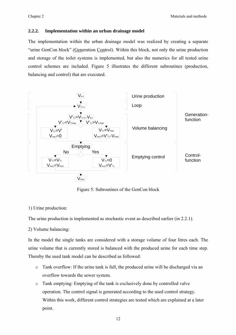
2.2.2. Implementation within an urban drainage model
The implementation within the urban drainage model was realized by creating a separate
“urine GenCon block” (Generation Control). Within this block, not only the urine production
and storage of the toilet systems is implemented, but also the numerics for all tested urine
control schemes are included. Figure 5 illustrates the different subroutines (production,
balancing and control) that are executed.
VT,i=0Vout,i=V'T,i
VT,i=Vmax
Vout,i=V'T,i-Vmax
Vout,i
VT,i=VT,i
Vout,i=Vout,i
V'T,i<VT,max
VT,i=V'Vout,i=0
V'T,i=VT,i-1+Vin,i
Emptying
V'T,i>VT,max
No Yes
VT,i-1
Vin,i Urine production
Emptying control Control-function
Loop
Volume balancing
Generation-function
Figure 5: Subroutines of the GenCon block
1) Urine production:
The urine production is implemented as stochastic event as described earlier (in 2.2.1).
2) Volume balancing:
In the model the single tanks are considered with a storage volume of four litres each. The
urine volume that is currently stored is balanced with the produced urine for each time step.
Thereby the used tank model can be described as followed:
o Tank overflow: If the urine tank is full, the produced urine will be discharged via an
overflow towards the sewer system.
o Tank emptying: Emptying of the tank is exclusively done by controlled valve
operation. The control signal is generated according to the used control strategy.
Within this work, different control strategies are tested which are explained at a later
point.

Chapter 2 Materials and methods
13
3) Emptying control
For the used control options a limitation regarding the tank features is applied. Thereby it is
assumed, that a tank, respectively the control unit which is installed, may receive signals, but
does not send any signal. Thus, for none of the tested control strategies, information on the
tanks current states (e.g. filling degrees) was available. If the control unit sends an emptying
signal to the receiver that is installed at the toilet, the tank of the separation toilet should be
emptied. The occurrence of an emptying signal depends on the urine control options (UCO)
which are illustrated in chapter 2.3. Figure 6 shows the GenCon block as implemented and the
underlying structure. The subroutines urine production and volume balancing are executed in
the generation function and the emptying control is executed in the control function.
Urine as ammonium sources
Load [g NH4/s]representing 20% of ammonium
representing 80% of ammonium
Load [g NH4/s]
C [g NH4/m3]Load/Q
C [g NH4/m3/(PE/WC) urine]
Ratio of ammonium loadOther ammonium / ammonium in urine
Other ammonium sources based on urine hydrograph
1DWF [m³/s,g/m³]
Urine GenCon
dwfrQDRr+ (dt)
DWF
PE
0.25
UAC
1dwf [m³/s/PE]
GenCon block submask
GenCon block
4t(+ dt) [m³/s]
3QDR [m³/s]
2rain [m³/s]
Generation function
Control function Generation function
Figure 6: Mask of the GenCon block
The following dynamic input signals are required for the GenCon block:
o dwf [m³/s/PE]…dry weather flow hydrograph scaled to unity regarding the PE
(population equivalent)
o r [mm/Dt]… the rainfall data as used for input to the model ( assumed online
measurement)
o QDR [m³/s]… effluent flow from a specific combined sewer overflow (CSO)
o r (t+Dt) [mm/Dt]…forecasted rainfall used for the interception control.

Chapter 2 Materials and methods
14
Static required inputs are entered via the block mask (see Figure 7).
2240
0.004
1
[1 1]
0.1
[0 7200 14400 21600 ... 86400]
[1.0 0.5 0.8 0.6 ... 1.0]
[0 7200 14400 21600 ... 86400]
[1.0 1.5 1.2 1.4 ... 1.0]
Population equivalent
Ammonium (NH ) concentration in urine [g /m ]4 NH4 URINE3 /(Pers/WC)
Toilet tank volume [m ]3
Number of pollutant components (n_comp=1) carried
Code for control option desired to apply
Flow for control options (used at ICO 2 for QDR)
Time steps used for generation of ammonium pollutograph [s]
Ammonium pollutograph y[g/m³]
Probability density function (PDF) (for BCO 3, only)
Time steps used for generation of PDF [s]
(explained later)
Figure 7: Block mask of GenCon block for static input parameters
In case several blocks are used, the input can either be entered for each block by using
globally parameters or by direct musk input.
Figure 6 shows that there are two paths for the generation of the output dry weather flow
(DWF). The first path generates the ammonium load of the urine volume, which is
representing ~80% of the total ammonium load. Only this source of ammonium can be
affected by the control option discussed here. The second path generates the ammonium load
of other sources (primarily “black water”) and represents ~20% of the total ammonium load.
Quantities from both sources (urine and non-urine stream) are related to each other via their
fraction percentage 80% : 20% = 1.00 : 0.25.
It is as well assumed that the ammonium load of other sources also follows the ammonium
pollutograph, but the ammonium load of other sources is not subjected to any control action
(thus no control block is used prior the Generation function block).

Chapter 2 Materials and methods
15
After adding both ammonium load streams the respective concentration in the dry weather
flow (dwf) is required. Utilizing the hydraulic flow of dry weather qDWF [m³/s] the respective
concentration is calculated as:
[ ]³/44
4 mgqMC NH
DWF
NHDWFNH =− ( 10 )
Output from both generation paths is the sum of urine discharged for a time step, based on the
number of toilets in the system. Therefore, the output represents the total catchment, but is
scaled – in average - by the expectation value ε(PWC). The scaled output is caused by the
stochastical algorithm of the urine generation.
To compensate the scaled output the urine ammonium concentration (UAC
[gNH4/m³Urine/(PE/WC)]) has to be multiplied with the expectation value ε(PWC)=1.6815.
As shown later, the UAC was used to calibrate the system.
The output signal of the GenCon block is the dry weather flow including the ammonium
concentration (DWF) [m³/s,g/m³].
2.3. TESTED CONTROL STRATEGIES
As described earlier, the effectiveness of different control strategies are tested regarding
diverse aims. A schematic overview is presented in Figure 8. Following the different weather
conditions (dry and wet weather), the strategies comprise of basic control options (BCO) and
interceptive control options (ICO).
The basic control options (BCO) are the main control options which – primarily – aim to
satisfy the goal of a more continuous ammonium load pollutograph at the WWTP.
If this control options are used exclusively, the overflow loads at CSOs will not be reduced.
Thus an interceptive control option (ICO) is designed to handle the reduction of ammonium
loads (peaks) in CSO overflow and rivers. Goal is to reduce the urine release during or prior
rain events such, that less ammonium is in the sewer system. Consequently this shall lead to a
reduction in overflow loads.
The basic control options (BCO) in connection with the interceptive control options (ICO)
result in the urine control options (UCO).
(BCO) + (ICO) (UCO)
Chapter 2 Materials and methods
16
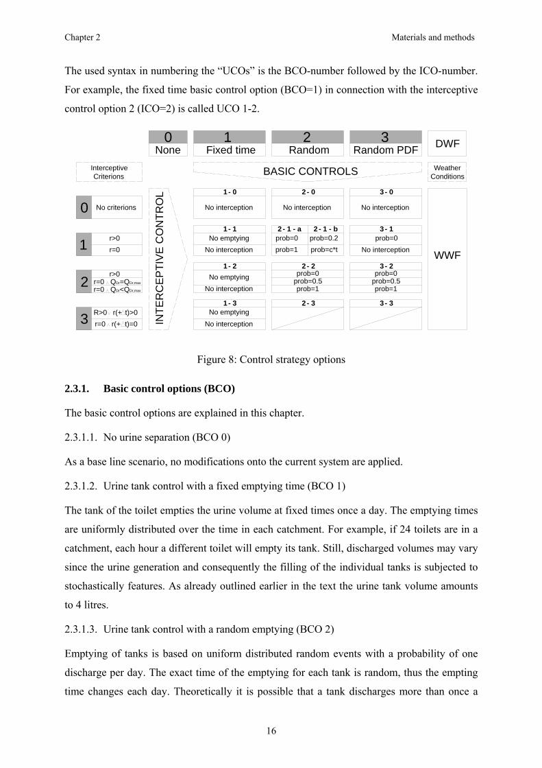
The used syntax in numbering the “UCOs” is the BCO-number followed by the ICO-number.
For example, the fixed time basic control option (BCO=1) in connection with the interceptive
control option 2 (ICO=2) is called UCO 1-2.
None Fixed time Random PDFRandom
WeatherConditions
Interceptive Criterions
DWF
No criterions
r=0r>0
r=0 QDr<QDr,max
r>0r=0 QDr=QDr,max
R>0 r(+ t)>0r=0 r(+ t)=0
WWF
INTE
RC
EP
TIV
EC
ON
TRO
L
No interception No interception No interception
No emptyingNo interception
No interception
No interception
No interception
No emptying
No emptying
prob=0.2prob=0prob=c*t
prob=0prob=1
prob=1 prob=1prob=0.5 prob=0.5
prob=0prob=0
BASIC CONTROLS
3210
0
1
2
3
1 - 0 2 - 0 3 - 0
3 - 11
- 1 2
- 1 - a 2 - 1 - b
1 - 2 2 - 2 3 - 2
1 - 3 2 - 3 3 - 3
Figure 8: Control strategy options
2.3.1. Basic control options (BCO)
The basic control options are explained in this chapter.
2.3.1.1. No urine separation (BCO 0)
As a base line scenario, no modifications onto the current system are applied.
2.3.1.2. Urine tank control with a fixed emptying time (BCO 1)
The tank of the toilet empties the urine volume at fixed times once a day. The emptying times
are uniformly distributed over the time in each catchment. For example, if 24 toilets are in a
catchment, each hour a different toilet will empty its tank. Still, discharged volumes may vary
since the urine generation and consequently the filling of the individual tanks is subjected to
stochastically features. As already outlined earlier in the text the urine tank volume amounts
to 4 litres.
2.3.1.3. Urine tank control with a random emptying (BCO 2)
Emptying of tanks is based on uniform distributed random events with a probability of one
discharge per day. The exact time of the emptying for each tank is random, thus the empting
time changes each day. Theoretically it is possible that a tank discharges more than once a

Chapter 2 Materials and methods
17
day or in quick succession as well. Thus, single tanks may be released when they are already
empty or may be not released for more than a day and thus generate an overflow.
2.3.1.4. Urine tank emptying with a probability distribution function (BCO 3)
The urine tank emptying is again randomly distributed, but it is based on a probability
distribution function (PDF). To follow the PDF over the time, a probability of ten discharges
per toilet and day is used. The density function itself is derived as reciprocally proportional to
the ammonium load pollutograph (see Figure 4) to counteract the usual daily variation.
Similar to BCO 2, the single urine tanks could discharge the urine volume in quick
succession.
2.3.2. Interceptive control options (ICO)
To approach the reduction of ammonium peaks in rivers, the basic control (BCO) is
interrupted by interceptive control options (ICO). The interception control criterions are:
1) interruption of BCO only during rain events (from start to end)
2) interruption at rain events and if a maximum effluent flow (QDR,max) at a specific
combined sewer overflow is reached. Thus, the interception of urine release strategies
is temporally extended at the end.
3) interruption at rain events and if a “rain forecast r(t+Dt)” announces an upcoming rain
event. The rain forecast which is used here is assumed to be perfect without any
uncertainties associated. Forecast horizon is 1.5 hours resulting in a 1.5 earlier
interruption of the BCO.
2.3.3. Urine control options (UCO)
Depending on the BCO the interceptive control is different although the same criterion
initiating the interruption is used. The different interceptive control options (ICO) applied
onto different BCOs are explained in the following.
2.3.3.1. Fixed time control in connection with interceptive control (UCO 1-i)
If the basic control is not interrupted (UCO 1-0), only the aim of a continuous ammonium
load pollutograph at the (WWTP) will be pursued. The advantage is that this strategy does not
need a signal from a central station. The disadvantage is that the CSO ammonium load into
the rivers is not significantly reduced.

Chapter 2 Materials and methods
18
The interceptive control options used in UCOs UCO 1-1, 1-2 and 1-3 result that urine is not
released, but buffered in the tanks. Thus a maximum of 4 litres urine per toilet and rain event
can be retained. In case of single tanks reaching the maximum fill, overflow is produced and
discharged towards the sewer system. For these UCOs a signal from a central station is
needed.
Fixed time1
1 - 0
1 - 1
1 - 2
1 - 3
No interception
No emptyingNo interception
No interception
No interception
No emptying
No emptying
0 No criterions
r=0r>01
2r=0 QDr<QDr,max
r>0r=0 QDr=QDr,max
r>0 v r(+ t)>03 r=0 r(+ t)=0
r
r(+ t)
QDr
time
time
time
Figure 9: Fixed time control in connection with interceptive control options
2.3.3.2. Random control in connection with interceptive control (UCO 2-i)
If the basic control is not interrupted (UCO 2-0), only the aim of a continuous ammonium
load at the (WWTP) will be pursued. This control option does not necessarily need a signal
from a central station.
If (UCO 2-1-a) the basic control is interrupted caused by criterion 1-a, the basic probability
for the emptying used in the BCO 2 will change abrupt to zero at the start of a rain event. For
UCO 2-1-b the probability is set to the interceptive probability 0.2/day. At the end of the rain
event, the probability is set to the uninterrupted state. Where for UCO 2-1-a the return to a
probability of 1 is too sudden, a more linear increase is applied in UCO 2-1-b. At the end of
the rain event the interceptive probability is set to 0.5/day and increasing steadily up to
1.0/day within the following 2 days. The approach applied in UCO 2-1-a is taken from Rauch

Chapter 2 Materials and methods
19
et al. (Rauch et al., 2002), where the underlying idea is to avoid an overload of the WWTP
with stored ammonium after rain events.
In control strategy UCO 2-2 the emptying of the tanks is not executed at rain events. If the
maximum effluent flow (QDR,max) of a combined sewer overflow (CSO) is reached in a dry
period, the interceptive probability of emptying is set to 0.5/day. After this period, the
emptying probability is set back to the initial probability of 1.
Interception criterion three (ICO 3) is not applied for the BCO 2.
Random2
2 - 0
2 - 1 - a
2 - 2
No interception
prob=0prob=1
prob=1prob=0.5prob=0
0 No criterions
r=0r>01
2r=0 QDr<QDr,max
r>0r=0 QDr=QDr,max
r
QDr
time
time
2 - 1 - bprob=0.2prob=c*tr=0
r>01
Figure 10: Random control in connection with interceptive control options with r (rain), QDR (effluent flow of CSO structure) and prob (interceptive probability)
2.3.3.3. Random PDF in connection with interceptive control (UCO 3-i)
If the basic control is not interrupted (UCO 3-0), only a continuous ammonium load at the
WWTP will be pursued. This control option does not need a signal from a central station.
If the basic control is interrupted, the interceptive probability of a tank emptying is set back to
zero at a rain event (UCO 3-1). Thereby a reduced ammonium emission into the river is
reached.
In control strategy UCO 3-2, at rain events, the emptying of the tanks is not executed. If the
maximum effluent flow (QDR,max) of a combined sewer overflow (CSO) is reached in a dry

Chapter 2 Materials and methods
20
period the interceptive probability of emptying is set to 50% of the basic probability (10
emptyings per day in connection with the probability distribution function).
Random PDF3
3 - 0
3 - 1
3 - 2
No interception
No interceptionprob=0
prob=1prob=0.5prob=0
0 No criterions
r=0r>01
2r=0 QDr<QDr,max
r>0r=0 QDr=QDr,max
r
QDr
time
time
Figure 11: Random PDF control in connection with interceptive control options with r (rain), QDR (effluent flow of CSO structure) and prob (the interceptive probability)
2.4. QUALITY CRITERIONS OF URINE TANK CONTROL OPTIONS
In general three aspects are considered for evaluating the quality of the improvement gained
by a control measure. Comparison for all control options is made with regard to the reference
scenario that is the uncontrolled case 0-0.
Criterion 1 (CR 1) – Averaging indicator
First goal is to gain an averaging load at the WWTP inflow tending towards a
homogeneous flow to the plant in terms of ammonium load.
Criterion 2 (CR 2) – CSO emission indicator
Secondly, the measures are evaluated regarding their overflow quality – respectively
the improvement in overflow quality gained.
Criterion 3 (CR 3) – River immission indicator
Last - but not the less important - quality changes in the rivers themselves are
evaluated with respect to concentrations in the river.
A more detailed description of indicators is provided in the following.

Chapter 2 Materials and methods
21
2.4.1. Averaging of the ammonium load at WWTP (CR 1)
The physical parameter which is used here to evaluate the averaging of pollutants flowing into
the WWTP is the ammonium load mA [gNH4-N/s].
Under ideal conditions, a constant ammonium load would arrive at the WWTP throughout the
day, being equivalent to the mean loading derived from the daily variation. Thus, for the ideal
case no deviation between single ammonium loads and their average load would be observed
within a sampling period. To quantify the averaging of the pollutograph the absolute
deviations from their average may serve as an indicator. In order to quantify relative
improvement of a control option, the averaging is written dimensionless relative to the
averaging of the reference case.
∑
∑
−
−= N
iAiA
N
i
jA
jiA
mm
mmICriterion
00,
,
( 11 )
The reference scenario which is used is the uncontrolled case without any urine separation
applying. In formula 11 i is the actual time step [0 – N]. Index j denotes the UCO.
The criterion is not only applied under dry weather flow conditions, but as well for longer
periods including rain events.
2.4.2. Ammonium overflow load reduction at CSO (CR2 – Emission based)
The second aim is to reduce the discharge of ammonium from CSO. Thus, this criterion
applies at the emission side.
Considering a single overflow event at a specific CSO structure, different descriptive
parameters may be used. Herein overflow events are separated according to the rainfall
pattern. A dry period lasting longer than three hours is considered to separate rain events.
Within this dry period, the system is assumed to be empty again and to carrying dry weather
flow (DWF) exclusively.

Chapter 2 Materials and methods
22
Different parameters are used to characterise the single overflow events. All parameters are
based on mass flow m(t) [g/s] = Q(t) [m3/s] * C(t) [g/m3]. The following parameters are used
to characterize single events:
]/[,, sgm LKMAXGM …Maximum gliding mean of mass flow for a gliding interval
of ΔT=1hour
]/[, sgm LKMAX …Maximum peak of mass flow within the event
∫ ⋅=t
LKLK dtmeventgM ,, ]/[ …Mass flow within the event
In all three parameters the indices K and L denote the examined event and CSO structure
respectively.
In order to be able to compare different scenarios the number of descriptors has to be reduced.
The high number of overflow events, locations and different parameters which are available
prohibit a clear and straight forward judgment without aggregating the set of numbers. Goal is
to identify a single indicator as used earlier with criterion 1 (Averaging at the WWTP).
Derivation of a single parameter is shown exemplarily for the maximum gliding mean values LK
MAXGMm ,, . For each of the scenarios j, a mean and maximum value was calculated regardless
the spatial and temporal distribution of overflow events.
[ ]LKMAXGM
jMAXGM mmeanm ,
,, = ( 12 )
[ ]LKMAXGM
jMAXMAXGM mm ,
,,
, max= ( 13 )

Chapter 2 Materials and methods
23
Both are illustrated in Figure 12. It can be seen, that both follow the same pattern with regard
to different UCO.
0-0 1-0 1-1 1-2 1-3 2-0 2-1a 2-1b 2-2 3-0 3-1 3-2
UCO a-b
m
a-b
[g/s
]G
M,M
AX
mean of UCO
m - Maximum gliding mean GM,MAX
m GM,MAX
0
0.1
0.2
0.3
0.4
0.5
0.6
0.7
0.8
Figure 12: Event based maximum gliding means for ammonium mass flow (means and maximums of UCO)
The maximum of the gliding mean is not needed as information for deriving a single
indicator, because the pattern of the mean value is similar. Mean values are normalized with
regard to the reference scenario.
0,
,,,
MAXGM
jMAXGMNj
MAXGMmmm = ( 14 )
To verify the normalized mean values as indicator, an alternative indicator has been used to
characterise the improvement. Thereby all CSO events of a specific urine control option (j)
are plotted against the corresponding data of the reference scenario (0-0). (see Figure 13).

Chapter 2 Materials and methods
24
In Figure 13 the event based maximums of ammonium overflow load are plotted against the
event based maximums of ammonium overflow loads of the reference scenario for each UCO.
0.1 0.2 0.3 0.4 0.5 0.6 0.7 0.80
0.1
0.2
0.3
0.4
0.5
0.6
0.7
0.8
m
a-b
[g/s
]G
M,M
AX
m 0-0 [g/s]GM,MAX
0
m - Maximum gliding mean GM,MAX
(1-2)(1-1)(1-3)(2-2)(2-1)(2-1b)
(0-0) - Reference sc
enario
m GM,MAX
K
Gradient of lin. regression
Maximum of eventRegression analysis
Linear regression for UCO vs. 0-0 scenarioK
Incr
easi
ngim
prov
emen
t
1-K Indicator of improvement
Incr
easi
ngim
prov
emen
t
Figure 13: Linear regression analysis of event based results plotted against the baseline scenario
The regression analysis of the plotted points results in a regression line. The gradient of the
regression line represents the improvement of each UCO. Low gradients indicate a fine
improvement. Regarding the reference scenario (actual state) the relative improvement can be
written as 1-K for each UCO.
This procedure being present for event based gliding means is done as well for event
maximums ]/[, sgm LKMAX and cumulated overflow masses ]/[, eventgM LK . These leads to
finally six parameters describing in the same fashion the improvement gained for each urine
control option.
Table 1: Single indicators used in criterion II
Gliding mean ][,
, −Nj
MAXGMm ( )0,,,
,,,, , LK
MAXGMjLK
MAXGMj
MAXGM mmfk =
Maximum ][,
−Nj
MAXm ( )0,,,, , LKMAX
jLKMAX
jMAX mmfk =
Cumulated overflow mass ][
,−
NjM ( )0,,,, , LKjLKj MMfk =

Chapter 2 Materials and methods
25
Cumulating to a single indicator is done by applying the arithmetic mean to the six parameters
which are shown.
( )jjMAX
jMAXGM
NjNjMAX
NjMAXGM kkkMmmIICriterion +++++= ,
,,,,
61 ( 15 )
2.4.3. In stream ammonium peak concentration (CR3 – Immission based)
Ammonium in water exists in two species (Unionized NH3-N and ionized NH4-N) where fish
toxicity is attributable to the unionized ammonia. However due to the two ammonium species
being in equilibrium in water, immission based assessment can be made using ammonium
(NH4-N).
With regard to toxic effects, in stream concentrations are more important than long term mass
balances. Thus, immission based comparisons between UCO based on in stream
concentrations. Since toxicity depends not only on concentration levels, but as well on
duration of exposure, such approaches are as well included in derivation of an indicator value.
The procedure to indicate the emission based situation is used in a modified form. In stream
concentrations (C) are used instead of mass flows (m). A dry period lasting longer than 24
hours is considered to separate rain events. Applying the procedure presented in 2.4.2 leads to
finally 4 parameters for each UCO denoting as:
Table 2: Single indicators used in criterion III
Gliding mean ][,
, −Nj
MAXGMC ( )0,,,
,,,, , LK
MAXGMjLK
MAXGMj
MAXGM CCfk =
Maximum ][,
−Nj
MAXC ( )0,,,, , LKMAX
jLKMAX
jMAX CCfk =
As an additional parameter the maximum concentration limit (max(c)) that is continuously
exceeded for minimum one hour in the evaluation period is used. This parameter accounts –
similar to the 1 hour gliding mean – for the exposure time, here taken to be one hour. Relating
this concentration level to the concentration level found in the reference scenario, leads to the
parameters in normalized form. Mathematically the parameter is defined as:
)()(:],[:))(max(: ,,0
,, ττχ
χχ
jjjNj
N
NjNj CtCttttCC ≤Δ+∈∀== ( 16 )

Chapter 2 Materials and methods
26
A schematic illustration can be found in Figure 14.
Ammonium pollutograph
Dt
C (
t) [g
/m3]
j
time t [s]
DtDt
Dt
Dt
DtC(t)j
max(C(t))j
C(t)j
C(t)j
C(t)j
Figure 14: Scheme to evaluate Cj,N
Again the different parameters are combined using the arithmetic mean of the totally 5 values
for each UCO.
( )NjjMAX
jMAXGM
NjMAX
NjMAXGM CkkCCIIICriterion ,
,,,
,51
++++= ( 17 )
2.4.4. Application of evaluation criterions
In the previous chapters, three different evaluation systems are presented, where each of them
leads to a single indicator.
2.4.4.1. Criterion I and II (Averaging and emission based criterion)
For criterion I temporal distributed data measured at the WWTP inflow has been cumulated to
a single indicator. By applying criterion II temporal and spatial distributed data has been
evaluated event based and cumulated again to a single indicator (see Formula ( 15 )).
2.4.4.2. Criterion III (Immission based criterion)
Criterion III is evaluated separate at different locations in the river system. The purpose of
immission based criterion is comparing it with criterion II (emission based criterion) to
substantiate the values of the criterions.
Chapter 3 Test scenario A - Virtual catchment
27
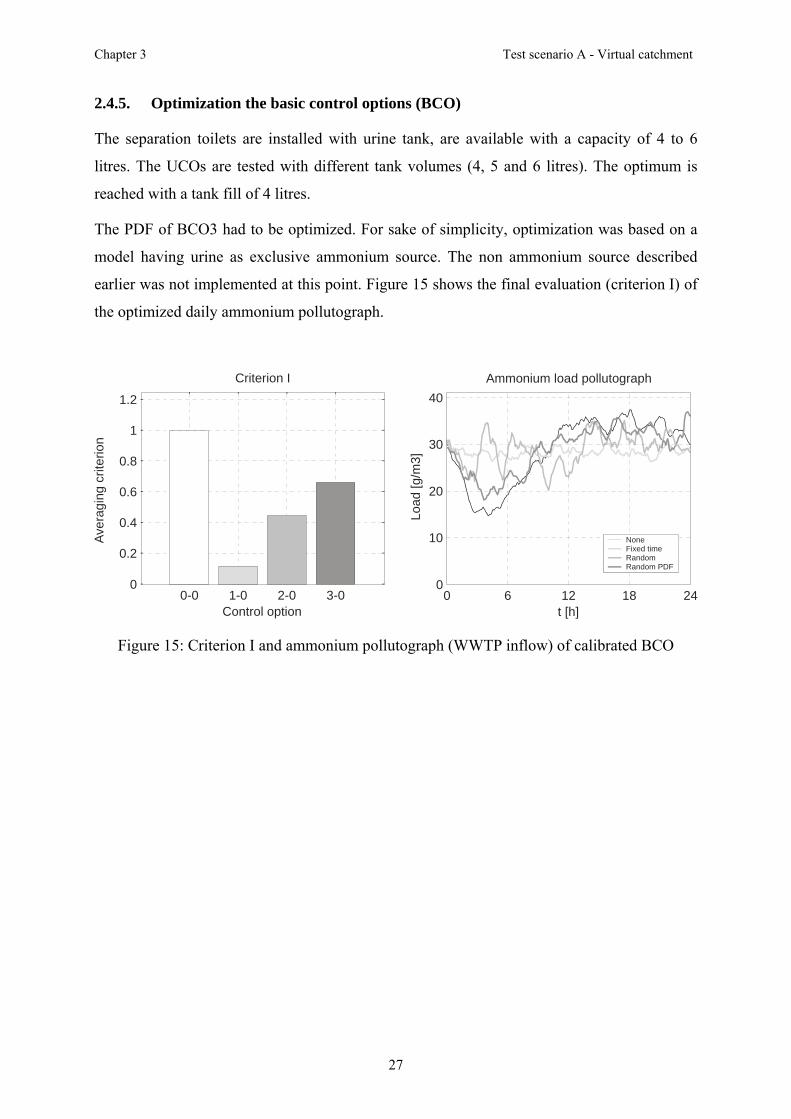
2.4.5. Optimization the basic control options (BCO)
The separation toilets are installed with urine tank, are available with a capacity of 4 to 6
litres. The UCOs are tested with different tank volumes (4, 5 and 6 litres). The optimum is
reached with a tank fill of 4 litres.
The PDF of BCO3 had to be optimized. For sake of simplicity, optimization was based on a
model having urine as exclusive ammonium source. The non ammonium source described
earlier was not implemented at this point. Figure 15 shows the final evaluation (criterion I) of
the optimized daily ammonium pollutograph.
0-0 1-0 2-0 3-00
0.2
0.4
0.6
0.8
1
1.2
Criterion I
Control option
Aver
agin
g cr
iterio
n
0 6 12 18 240
10
20
30
40Ammonium load pollutograph
t [h]
Load
[g/m
3]
NoneFixed timeRandomRandom PDF
Figure 15: Criterion I and ammonium pollutograph (WWTP inflow) of calibrated BCO

Chapter 3 Test scenario A - Virtual catchment
28
3. TEST SCENARIO A - VIRTUAL CATCHMENT
A single combined sewer catchment is defined for a preliminary study of the desired control
strategies.
As input for dry weather flow, a unit hydrograph (flow per PE) is used (same as used for the
main sewer Reutte in the next chapter). The rain gauge data of the station Reutte is used as
rain input.
The virtual catchment is defined having a population equivalent (PE) of 2,000 inhabitants, a
runoff area (A) of 100 ha and a runoff coefficient (f) of 0.15. The flow time (tf) in the
catchment is taken to be one hour (see CITY DRAIN model in Figure 16).
urine
Urine Parameters
Urine GenCon
dwf
r
QDR
r+ (dt)
DWF
Urine GenConRAIN READ
RAIN READ
Rainread
[rain]
[rain][rain]
dwf
wc
wc
CSO
Typ BQi
Qw
Qe
Vi
CSO
CITY DRAIN CITY DRAIN CITY DRAINCITY DRAINPARAMETERS PARAMETERS
PARAMETERSPARAMETERS
CD Parameters
rl
DWFl
Qpl
Qe
Qe
CATCHMENT CSS
Catchment CSS
Figure 16: Test scenario „virtual catchment“
Downstream the catchment a combined sewer overflow (CSO) is installed. The CSO basin
volume is 200 m³. Maximum effluent flow (QDR) is 0.04 m³/s. The ratio of A*(f)/VCSO is
approximately 15 m³/haRED in accordance to ÖWAV-RB19 (ÖWAV, 2006). Population
density which is applied is ~133 PE/haRED which is as well in feasible range.

Chapter 4 Test scenario B - Case study Vils-Reutte
29
4. TEST SCENARIO B - CASE STUDY VILS-REUTTE
Prior to the model implementation and testing, the collection and preparation of data for the
“Case Study Vils” is made. Based on a structured data, the case study can be modelled and
calibrated. The drainage area of the “AWV-Vils-Reutte und Umgebung” (AWV-Vils) is taken
as case study. Figure 17 gives an overview on the connected drainage area.
Figure 17: Map of the case study Vils-Reutte
The upstream end of the Vils catchment (northwest part) is ‘Pfronten’, a town in Germany. It
is located along the river Vils, which runs from ‘Pfronten’ down to the WWTP and later to
‘Weißenbach’. From the south, the river Lech flows from ‘Weißenbuch’ through ‘Reutte’
meeting with river Vils further downstream.
The region Reutte is situated 800 m to 900 m above sea level. The climate is alpine, so the
region is characterized by cold winters and summers with intense rainfalls. The population

Chapter 4 Test scenario B - Case study Vils-Reutte
30
equivalent (PE) of all the villages is about 40,000. The average flow time (tf) of the sewer
system amounts 3 hours. The runoff areas (A) are in sum roughly 1,000 ha with an average
runoff coefficient (f) of 0.12.
In the region, two main sewer systems are installed, delivering wastewater to the WWTP. In
the northwest the main sewer Vils connects the catchments (CA) of 2 villages. In this area 3
combined sewer overflows (CSO) and one inline storage volume are installed.
The main sewer Reutte in the south connects the catchments (CA) of 11 villages. There are 4
CSOs and 7 pumping stations (PS).
Figure 18: Schematic map of the catchment Vils-Reutte
Chapter 4 Test scenario B - Case study Vils-Reutte
31
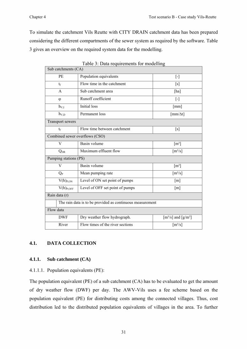
To simulate the catchment Vils Reutte with CITY DRAIN catchment data has been prepared
considering the different compartments of the sewer system as required by the software. Table
3 gives an overview on the required system data for the modelling.
Table 3: Data requirements for modelling Sub catchments (CA)
PE Population equivalents [-]
tf Flow time in the catchment [s]
A Sub catchment area [ha]
ϕ Runoff coefficient [-]
hV,I Initial loss [mm]
hV,D Permanent loss [mm/Δt]
Transport sewers
tf Flow time between catchment [s]
Combined sewer overflows (CSO)
V Basin volume [m³]
QDR Maximum effluent flow [m³/s]
Pumping stations (PS)
V Basin volume [m³]
QP Mean pumping rate [m³/s]
V(h)P,ON Level of ON set point of pumps [m]
V(h)P,OFF Level of OFF set point of pumps [m]
Rain data (r)
The rain data is to be provided as continuous measurement
Flow data
DWF Dry weather flow hydrograph. [m³/s] and [g/m³]
River Flow times of the river sections [m³/s]
4.1. DATA COLLECTION
4.1.1. Sub catchment (CA)
4.1.1.1. Population equivalents (PE):
The population equivalent (PE) of a sub catchment (CA) has to be evaluated to get the amount
of dry weather flow (DWF) per day. The AWV-Vils uses a fee scheme based on the
population equivalent (PE) for distributing costs among the connected villages. Thus, cost
distribution led to the distributed population equivalents of villages in the area. To further

Chapter 4 Test scenario B - Case study Vils-Reutte
32
estimate PE of sub catchment (parts of villages), the PE of a village has been distributed
according to the sub catchments areas.
4.1.1.2. Flow times (tf):
The software CITY DRAIN requires the flow time within a catchment. This is considered as
the maximum flow path of the waste water in a sub catchment (CA). Unfortunately, the
available sewer data only includes data of main sewers, but no data on regional sewers in a
sub catchment (CA). Secondly the flow time for runoff concentration can only be estimated.
Last, the waste water that originates from upper catchments – and is routed through the
system - has as well to follow the one pathway described by the flow time.
As an estimate the flow time (tf) of a sub catchment (CA) is considered as the sum of the flow
time (tf,1) in the main sewer that crosses the sub catchment (CA) (see Figure 19 - route AB)
and the flow time (tf,2) of the effluent flow from the furthermost point rectangular to the main
sewer (see Figure 19 - route PC).
The flow velocity of the route AB (the main sewer) was calculated. This was possible due to
available sewer data. Application of the Prandtl-Colebrook equation was based on the
assumption that the cross section is filled for ¾ of its height.
The flow time (tf,2) of route PC was evaluated assuming an average flow velocity of 1 m/s.
Figure 19: Scheme of theoretical flow routes within a sub catchment

Chapter 4 Test scenario B - Case study Vils-Reutte
33
4.1.1.3. Runoff areas (A):
The “Tiroler Raumordnungs-Informationssystem” (TIRIS) (Tyrolean information system on
regional development) provided an ortho photo of the region. On this basis it was possible to
– visually - define and digitize the boundaries of densely populated areas and its sub
catchments. Catchment areas were obtained using a CAD software.
4.1.1.4. Runoff coefficients (ϕ):
Runoff coefficients (f) for each sub catchment were estimated as well on basis of the ortho
photo. Parts of the sub catchments having visually different runoff coefficients (roads,
grass,…) were combined to a single (area) weighted runoff coefficient (ϕ).
4.1.1.5. Initial loss in the rain runoff (hv,i):
The initial loss (hv,i) depends on the depression storage and the hydraulic conductivity of the
ground. The value of 2.5 mm is situated in the middle of the spectrum [0.6, 5] mm found in
Lautrich (Lautrich, 1980).
4.1.1.6. Permanent loss of rain water (hv,d):
The permanent loss (hv,d) depends on the evaporation. The value of 1.25 l/d is assumed.
In Table 4 the data of totally 32 sub catchments located in the catchment Vils Reutte is
summarized. Overall, there is a total population of 37993 PE distributed over a total (gross)
area of 971 ha which is densely populated. 61 % of the PE and 54 % of the area A is
connected to a combined sewer system (CSS).

Chapter 4 Test scenario B - Case study Vils-Reutte
34
Table 4: Data of sub-catchments in the drainage Area Vils-Reutte Village # Catchment Type PE A tf ϕ hv,i hv,d [ha] [min] [-] [mm] [l/d]
Pfronten Pfronten 13105 211.6 1-1 Pfronten 1 CSS 1618 26.1 30 0.40 2.5 1.25 1-1-1 Pfronten 1-1 SSS 2556 41.3 30 0.40 2.5 1.25 1-2 Pfronten 1-2 CSS 4961 80.1 28 0.40 2.5 1.25V
ILS
1-3 Pfronten 1-3 CSS 3970 64.1 22 0.40 2.5 1.25Vils 2 Vils CSS 1731 94.5 22 0.52 2.5 1.25Pinswang SSS 485 19.5 3 Unterpinswang 295 11.8 33 0.55 2.5 1.25 4 Oberpinswang 190 7.6 20 0.58 2.5 1.25Musau SSS 374 23.0 5 Musau 256 15.8 29 0.51 2.5 1.25 6 Brandstatt 90 5.5 12 0.55 2.5 1.25 7 Roßschläg 28 1.7 3 0.60 2.5 1.25Pflach SSS 1277 59.4 8 Pflach O 781 36.3 28 0.50 2.5 1.25 9 Pflach W 496 23.1 31 0.45 2.5 1.25Reutte CSS 8289 187.5 10 Reutte N 3195 72.3 24 0.55 2.5 1.25 11 Reutte SW 2959 66.9 29 0.55 2.5 1.25 12 Reutte SO 2135 48.3 30 0.50 2.5 1.25Breitenwang 2728 101.1 13 Breitenwang CSS 814 30.2 33 0.50 2.5 1.25 14 Mühl SSS 1619 60.0 40 0.45 2.5 1.25 15 Lähn P CSS 150 5.5 7 0.65 2.5 1.25 16 Lähn L CSS 146 5.4 4 0.65 2.5 1.25Lechaschau 2148 79.9 17-1 Nord SSS 967 36.0 21 0.55 2.5 1.25 17-2 Süd SSS 1181 44.0 23 0.55 2.5 1.25Wängle 1394 35.2 18 Wängle CSS 1355 34.2 19 0.50 2.5 1.25 19 Holz CSS 39 1.0 6 0.60 2.5 1.25Ehenbichl 1521 31.1 20 Ehenbichl SSS 1138 23.3 20 0.50 2.5 1.25 21 Rieden SSS 383 7.8 14 0.65 2.5 1.25Höfen 1756 66.3 22 Höfen NW SSS 481 18.2 9 0.45 2.5 1.25 23 Höfen NO SSS 715 27.0 28 0.45 2.5 1.25 24 Höfen S SSS 560 21.1 15 0.55 2.5 1.25
RE
UT
TE
Weissenbach 25 Weissenbach SSS 1588 52.8 55 0.60 2.5 1.25 Heiterwang 26 Heiterwang SSS 707 27.6 24 0.50 2.5 1.25 Bichelbach 27 Bichelbach SSS 1264 5.0 6 0.50 2.5 1.3

Chapter 4 Test scenario B - Case study Vils-Reutte
35
4.1.2. Transport sewers
Transport sewers are defined as main sewers between sub catchments. There is no additional
waste water inflow along its flow path.
Figure 20: Scheme of flow routes between sub catchments
The flow velocity of the route AB was calculated based on sewer pipe data was available.
Application of the equation of Prandtl-Colebrook was based on the assumption that pipes are
filled up to ¾ of the maximum fill. Different sewer sections with changing cross sections
were considered in the calculations.
Table 5: Lengths (l) and flow time (tf) of transport sewers between sub catchments
ID l [m] tf [min] ID l [m] tf [min] ID l [m] tf [min]0-1 1200 16 8 1579 12 18 572 3
0-2 1800 25 9 281 4 19 2590 42
0-3 1400 12 10 1835 21 20 961 15
1 3169 28 11 496 6 21 630 8
2 1863 24 12 579 14 22 529 4
3 1453 13 13 385 5 23 1421 10
4 573 12 14 1038 16 24 277 5
5 1064 9 15 325 2 25 5257 87
6 323 3 16 762 8 26 4685 78
7 684 8 17 399 6

Chapter 4 Test scenario B - Case study Vils-Reutte
36
4.1.3. Combined sewer overflow structures (CSO)
Basin volumes (V) and maximum effluent flows (QDR) of each CSO structure were provided
by the “Planungsbüro Prantl”, a consulting engineer office, the AWV-Vils, and the municipal
office of Pfronten. Additionally measured overflow events of the CSO 1 were provided.
Table 6: CSO data CSO-ID V QDR [m³] [l/s]
1 800 3152 280 3253 134 22
RE
UT
TE
4 270 605 800 906 300 357 74 6V
ILS
8 200 80
4.1.4. Pumping stations (PS)
Besides the storage (basin) volumes (V) of each pumping station, pump characteristics such
as fixed (mean) pumping rates QP and ON / OFF set-points were assessed.
In all pumping stations only one pump was used – although the software CITY DRAIN is
capable of simulating multiple pumps. Usually, the pump rate of pumps depends on the pump
head which is to overcome.
A constant pump rate QP was estimated by the ratio QP/HP. The pump head HP was taken as
the difference of start- and end level of the pressure line including the head loss resulting from
friction. The water level in the basin was neglected.
The OFF and ON set points (hoff, hon) of the pumping station are transferred to volumes (Von,
Voff).
Recorded operating hours of the pump of the PS 1 were provided by the AWV-Vils.
Table 7: Pumping station data PS-ID Pumping Station Sewer QP Voff Von V [m³/s] [m³] [m³] [m³]
1 Klosterweg 02 0.175 - - 18.50 2 Rieden 08 0.008 0.40 3.27 2.87 3 Musau 09 0.011 0.22 0.92 0.70 4 Roßschläg 09 0.009 0.23 0.91 0.68 5 Oberpinswang 10-1 0.011 0.40 2.71 2.31 6 Unterpinswang 10-2 0.011 0.40 2.85 2.45 R
EU
TT
E
7 Heiterwang 12 0.0110 - - 22.15

Chapter 4 Test scenario B - Case study Vils-Reutte
37
4.1.5. Rain data (r)
The rain data was provided as cumulated volumes [mm/m²] for 10 minute time intervals. The
available data was a continuous long term series from 1998-2004 (UTC time scale) provided
by National Meterological Institute ZAMAG („Zentralanstalt für Meteorologie und
Geodynamik“). The ammonium concentration of water in storm water pipes was taken to be
1 g NH4/m³ according to data records found in Brombach and Fuchs (Brombach and Fuchs,
2003).
4.1.6. Flow data
4.1.6.1. Dry weather flow
The aim was to calibrate the sewer system model using original dry weather flow data. Thus,
an inflow hydrograph at the WWTP for dry weather conditions was evaluated on basis of an
inflow data series from Jan. – Oct. 2004. Data was provided as 15 minute mean values
measured at the WWTP inflow. Different daily hydrographs were averaged to single
representative hydrographs. Thereby, only days without precipitation on the day before and
on the corresponding day were used. This was to exclude the influence of previous rainfalls
onto flow measurement.
An analysis of hydrographs in tourist season reveals that the DWF does not change
significantly compared to regular seasons. A different pattern will be seen, if workdays (Mon-
Fri) are compared with the weekend (Sat-Sun). Therefore a dry weather flow hydrograph was
composed for workdays and weekends, separately.
Flow measurements at the WWTP were made separate for the two main sewers Reutte and
Vils, resulting in a separate assessment of each.
For preparing the data, the time data had to be corrected for UTC (Coordinate Universal
Time). Reason was that the time scales which was used was the MEWT (Middle European
Winter Time) and the MEST (Middle European Summer Time), respectively. In order to have
a uniform – and continuous - time scale throughout the year, both MEWT and MEST were
corrected for UTC with +1 and +2 hours, respectively.
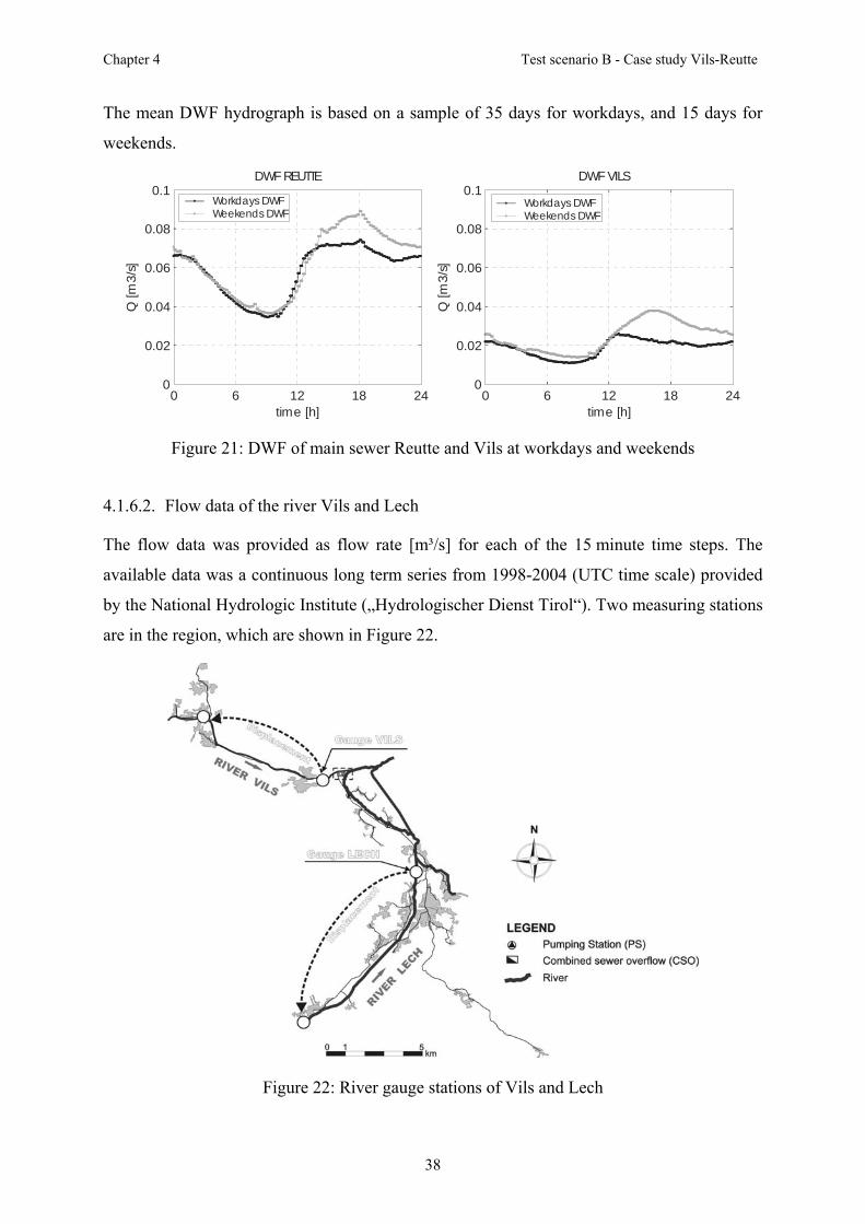
Chapter 4 Test scenario B - Case study Vils-Reutte
38
The mean DWF hydrograph is based on a sample of 35 days for workdays, and 15 days for
weekends.
0 6 12 18 240
0.02
0.04
0.06
0.08
0.1DWF REUTTE
time [h]
Q [m
3/s]
0 6 12 18 240
0.02
0.04
0.06
0.08
0.1DWF VILS
time [h]
Q [m
3/s]
Workdays DWFWeekends DWF
Workdays DWFWeekends DWF
Figure 21: DWF of main sewer Reutte and Vils at workdays and weekends
4.1.6.2. Flow data of the river Vils and Lech
The flow data was provided as flow rate [m³/s] for each of the 15 minute time steps. The
available data was a continuous long term series from 1998-2004 (UTC time scale) provided
by the National Hydrologic Institute („Hydrologischer Dienst Tirol“). Two measuring stations
are in the region, which are shown in Figure 22.
Figure 22: River gauge stations of Vils and Lech

Chapter 4 Test scenario B - Case study Vils-Reutte
39
For modelling purpose, gauge measurements from downstream were displaced and used as
upstream input. Comparison of downstream measured flows and modelled flows (incl.
displacement) are nearly identical.
At these stations the flow velocity is measured as well, but only once a month. The flow
velocities were averaged to estimate the flow time. Rain water from separate sewer systems
sub catchments (CA), combined sewer overflows (CSO), waste water of emergency spillway
of the pumping stations (PS) and the outflow of the waste water treatment plant (WWTP)
discharge polluted water into the river sections.
Table 8 and Figure 23 give an overview on the river stretches and the discharge points which
are defined.
Table 8: River data
Section l v t [m] [m/s] [min]
7-3-1 1500 0.79 307-3-2 5000 0.79 1057-3-3 1210 0.79 253-4-1 1232 0.79 25VI
LS
3-4-2 500 0.79 104-5 1238 0.60 35 6-1-4 2000 1.23 256-1-3 3956 1.23 556-1-2 2000 1.23 256-1-1 2000 1.23 251-2 3174 1.23 452-4-2 3100 0.30 1702-4-1 2805 0.30 155
LEC
H
2-5 4392 1.23 60
Figure 23: River scheme and inflow points

Chapter 4 Test scenario B - Case study Vils-Reutte
40
Based on a measurement report made by the IUT (Unit of Environmental Engineering) the
ammonium concentration of the river Vils was taken to 0.016 g NH4/m³ (see Figure 23 P7)
and the ammonium concentration of the river Lech was taken to 0.02 g NH4/m (see Figure 23
P6).
4.2. MODEL CALIBRATION
After the data collection, the case study Vils is modelled with CITY DRAIN (see Figure 24).
Using the model the collected parameters were included as a starting point for further
calibration. Hydraulics as well as ammonium were calibrated in the base line scenario.

Chapter 4 Test scenario B - Case study Vils-Reutte
41
Figure 24: Scenario B – City Drain model of catchment Vils Reutte

Chapter 4 Test scenario B - Case study Vils-Reutte
42
4.2.1. Indicators for calibration quality
To evaluate the quality of the calibration, quality indicators are defined to compare the
measured data (M) with the simulated data (S). The indicators shown in the following are
taken from M. Grecu, W.F. Krajewski (Grecu and Krajewski, 2000).
4.2.1.1. Correlation coefficient (C)
The correlation coefficient (C) compares the total variance of the two independent variables.
Thus, this value is not suitable to compare measured data (M) with simulated data (S) since
(C) represents the quality of a linear regression. Additionally the correlation coefficient (C) is
not sensitive enough to differentiate proportional between the measured data (M) and
simulated data (S). Thus the correlation coefficient is not applied.
4.2.1.2. The coefficient of efficiency (E)
The coefficient of efficiency (E) is defined as
∑
∑
=
=
−
−−= N
ii
N
iii
MM
SME
1
2
2
1
)(
)(1 ( 18 )
The interval of E ranges from minus infinity (-∞) to 1. A larger value indicates a better
agreement. If E is less than 0, the simulated data (S) matches worse than the mean value of
the measured data.
4.2.1.3. Index of agreement (d)
The index of agreement (d) ranges from 0 to 1. A large value indicates a good agreement.
2
1
2
1
)(
)(1
∑
∑
=
=
−+−
−−= N
iii
N
iii
MSMM
SMd ( 19 )

Chapter 4 Test scenario B - Case study Vils-Reutte
43
4.2.1.4. The multiplicative bias (B)
The bias (B) evaluates the ratio of the means.
MSB = ( 20 )
4.2.2. Calibrating the dry weather flow (DWF)
The catchment blocks in the simulation environment utilize the dry weather flow (DWF)
pattern as dynamic input, which had to be evaluated. The objective was to create a simulated
dry weather inflow to the WWTP which is – as far as possible – similar to the measured
pattern.
Measurements are limited to the WWTP inflows from the main sewers Vils and Reutte.
At the catchment level a unit waste water hydrograph (per PE) was used, scaled by the daily
mean DWF to calibrate magnitudes. For the unit DWF hydrograph a cubic spline with 6 data
points was used which has an area of 1 under the curve. Modifying the unit hydrograph
allowed to fit the daily variation without changing daily mean flow magnitude (pattern
calibration). In absence of better knowledge, the same pattern was used in all sub catchments.
Points were varied such that simulation produced the correct shape and magnitude of flow at
the WTTP. This was done for the main sewer systems Vils and Reutte, for workdays and for
weekends.
0 6 12 18 240
0.02
0.04
0.06
0.08
0.1
time [h]
Q [m
3/s]
0 6 12 18 240
0.04
0.06
0.08
0.1DWF REUTTE - Weekends
time [h]
Q [m
3/s]
DWF MeasuredDWF Simulated
0.02DWF MeasuredDWF Simulated
DWF REUTTE - WorkdaysE= 0.97d= 0.99B= 1.01
E= 0.97d= 0.99B= 1.01
Figure 25: Simulated and measured DWF hydrographs main sewer Reutte

Chapter 4 Test scenario B - Case study Vils-Reutte
44
The daily waste water volume in sub catchments according to the FAAT (ÖWWV, 1982)
amounts 200 l/PE (value for design). Having this mean daily DWF as starting point, the
calibrated mean of the daily DWF at the main sewer Reutte came out to be 213 l/PE. This
calibrated value is in the order of magnitude with the recommended value for design purpose
of the guideline.
E= 0.96d= 0.99B= 1.02
DWF MeasuredDWF Simulated
0.02
0 6 12 18 240
0.02
0.04
0.06
0.08
0.1DWF VILS - Workday
time [h]
Q [m
3/s]
0 6 12 18 240
0.02
0.04
0.06
0.08
0.1DWF VILS - Weekends
time [h]
Q [m
3/s]
DWF MeasuredDWF Simulated
E= 0.97d= 0.99B= 1.00
Figure 26: Simulated and measured DWF hydrographs main sewer Vils
The calibrated mean DWF in sub catchments at the main sewer Vils amounts 111 l/PE. The
difference to the guideline value is the result of a little water demand of the village Vils,
which amounts 63 l/PE/day. In contrast to the water demand of the village Vils, the water
demand of the village Reutte amounts 154 l/PE/day (design value 150 l/PE/day (ÖWWV,
1982)). The water demand values were taken from the payment scheme that has been
provided by the AWV-Vils.
4.2.3. Calibrating the wet weather flow (WWF)
Within CITY DRAIN it is as well possible to cover rainfall runoff processes. Precipitation is
thereby drained either via combined sewer pipes (towards the WWTP) or storm sewer pipes
(discharged to the river). To calibrate the wet weather flow (WWF), which is the
superposition of calibrated DWF and rainfall runoff, an observation period of 72 days of the
year 2004 (August – October) was used. The objective was to create a simulated inflow of the
WWTP which meets the measured flows with least possible error.

Chapter 4 Test scenario B - Case study Vils-Reutte
45
The model parameters which were modified to calibrate the system are:
o the runoff coefficient (f) and the initial loss (hv,i) of the catchment blocks to handle
the amount of the wet weather flow hydrograph,
o the maximum effluent flow (QDR) of the CSO to handle maximum flows delivered
downstream,
o and the number of sub reaches of the sewer blocks to handle the flow time (tf) of the
sewer system.
Optionally, the parameter X of the muskingum sewer software block can be modified, for a
fine tuning of the calibration. Finally this option was not used, because it would – in this case
- not result in a significant improvement of the calibration.
To quantify the calibration quality using the quality indicators shown earlier, the measured
data and simulated data were separated for different rain events. A rain event is thereby
defined as an interval, where rainfall (r) is not interrupted longer than 3 hours (mean flow
time of the main sewer Reutte). In Figure 27 and Figure 28, the simulated maximum flow rate
(QMAX) and waste water volume (V) of each rain event were compared with the measured
values.
The quality indicators coefficient of efficiency (E), index of agreement (d) and the
multiplicative bias (B) were calculated for the maximum flow rates (QMAX).
Main Sewer Reutte
0 0.05 0.1 0.15 0.2 0.250
0.05
0.1
0.15
0.2
0.25
QMAX Measured [m3/s]
QM
AX S
imul
ated
[m3/
s]
0 2e3 4e3 6e3 8e3 10e30
2e3
4e3
6e3
8e3
10e3
V Measured [m3/event]
V Sim
ulat
ed [m
3/ev
ent]
Main Sewer ReutteE= 0.74d= 0.93B= 0.94
E= 0.97d= 0.99B= 0.98
Figure 27: QMAX and volume ratio of main sewer Reutte

Chapter 4 Test scenario B - Case study Vils-Reutte
46
The quality indicators coefficient of efficiency (E), index of agreement (d) and the
multiplicative bias (B) were calculated for the volumes (V).
0 0.05 0.1 0.15 0.20
0.05
0.1
0.15
0.2
QMAX Measured [m3/s]
QM
AX S
imul
ated
[m3/
s]
0 1e3 2e3 3e3 4e3 5e30
1e3
2e3
3e3
4e3
5e3
V Measured [m3/event]V
Simul
ated
[m3/
even
t]
E= 0.51d= 0.85B= 0.85
E= 0.87d= 0.97B= 0.99
Main Sewer Vils Main Sewer Vils
Figure 28: QMAX and volume ratio of main sewer Vils
The correlation of the main sewer Vils is less than the correlation of the main sewer Reutte.
This is due to two reasons:
o no rain data was measured near the villages of the main sewer Vils. The rain data that
was measured in the village of Reutte was also used to compute the rainfall runoffs of
the sub catchments (CA) in the main sewer system Vils.
o no longitudinal section of main sewer Vils was available thus the flow velocity was
estimated with 1 m/s.

Chapter 4 Test scenario B - Case study Vils-Reutte
47
In Figure 29 and Figure 30, a sample of a rain event with high rain intensity is plotted.
1.54 1.56 1.58 1.6
x 106
0
0.05
0.1
0.15
0.2
0.25
cd time [sec]
Q [m
3/s]
WWF MeasuredWWF Simulated
Sample WWF Reutte
E= 0.70d= 0.94B= 0.88
Figure 29: WWF sample of Rain event main sewer Reutte
1.54 1.56 1.58 1.6
x 106
0
0.05
0.1
0.15
0.2
cd time [sec]
Q [m
3/s]
WWF MeasuredWWF Simulated
Sample WWF Vils
E= 0.74d= 0.93B= 0.86
Figure 30: WWF sample of Rain event main sewer Vils
Additively, the simulated number of CSOs of the most important CSO structure (CSO 1) was
compared with the logged overflow data. Difficulties occur due to the data not being logged
regularly. Dealing only with data of the number of overflows allows only a very rough
estimation on events occurring or not, but allows no distinct calibration for overflow volumes.
The pumping station with the highest wet weather flow has a data logger which is measuring
the operating hours of the pumps. This data obtained thereby was compared to the pumping
rates of the simulation.

Chapter 4 Test scenario B - Case study Vils-Reutte
48
4.2.4. Calibrating the ammonium pollutograph
First of all, the daily ammonium load at the WWTP inflow was calibrated. The ammonium
concentration pollutograph of the urine was composed with a normalized 12 point polygon
(see Figure 31 Normalized ammonium pollutograph). The mean concentration of ammonium
in urine (UAC) was modified to obtain the correct magnitude of load (mean ammonium
concentration of simulated and measured data agreed). Since the UAC is – numerically –
scaled for the expectation value ε(PWC), the concentration is related to the number of PE/WC
present in a catchment. Measured ammonium concentration resulted from field measurements
by IUT (Unit of Environmental Engineering). The ammonium concentration was measured at
the 28.7.2005 having 2 hour composite samples. The calibrated mean urine concentration
UCA was
[ ])//(³/4240,2 WCPEmgNHUCA = ( 21 )
As the UCA value was used for calibration parameter, the urine concentration was
crosschecked with literature values of ammonium concentration in urine. UCA is to be scaled
by the expectation value of PWC.
( ) [ ]³/4770,36815.1240,24 mgNHPWCUCAC UNH =⋅=⋅=− ε ( 22 )
The urine ammonium concentration found in the literature (Jönsson et al., 1997) was in the
range of 3,600-3,900 [g NH4/m³]. Thus, the UCA value which is calibrated is in agreement to
literature data.
0 6 12 18 240
1
2
3
4
DWF ammonium pollutograph
time [h]
UA
C [g
/m3]
norm
NH
4
NH4 MeasuredNH4 Simulated
x 10-3Normalized ammonium pollutograph
0 6 12 18 24time [h]
0
10
20
30
40
NH
4 [g
/m3]
E=0.59d=0.85B=1.01
Sub catchment / Toilet scale WWTP
Figure 31: Ammonium pollutograph of a sub catchment and the WWTP inflow
The finally used model parameters fixed after calibration are summarized in the attachment.

Chapter 5 Results – Evaluation of control strategies
49
5. RESULTS – EVALUATION OF CONTROL STRATEGIES
The different urine control options were tested on scenarios A and B. Test scenario A
represents a virtual catchment with a short flow time and a homogeneously population
density. Test scenario B represents a real world sewer catchment with a large flow time and
an inhomogeneous population density.
5.1. TEST SCENARIO A - VIRTUAL CATCHMENT
Using the test scenario A the evaluation of the basic control options (BCO) in connection with
the interceptive control options (ICO) are tested for dry weather (DWF) and wet weather
(WWF) conditions.
5.1.1. Basic control options (BCO) at DWF
For dry weather conditions, only the aim of averaging the ammonium pollutograph at the
WWTP is relevant. Figure 32 shows the BCO evaluated for criterion I, the averaging criterion
0-0 1-0 2-0 3-00
0.2
0.4
0.6
0.8
1
1.2
Criterion I
Control option0 6 12 18 24
0
10
20
30
40
Ammonium load pollutograph
t [h]
Load
[g/m
3]
NoneFixed timeRandomRandom PDF
Aver
agin
g cr
iterio
n
Figure 32: Criterion of averaging; ammonium pollutograph (DWF, virtual catchment)
The fixed time control option (BCO 1) is found to be the optimum under these conditions.
The peaks observed at the uncontrolled ammonium load pollutograph will be nearly evened
out, if this control strategy is applied. The different filling degrees of the tanks at emptying
time causes fluctuations in the ammonium load pollutograph.
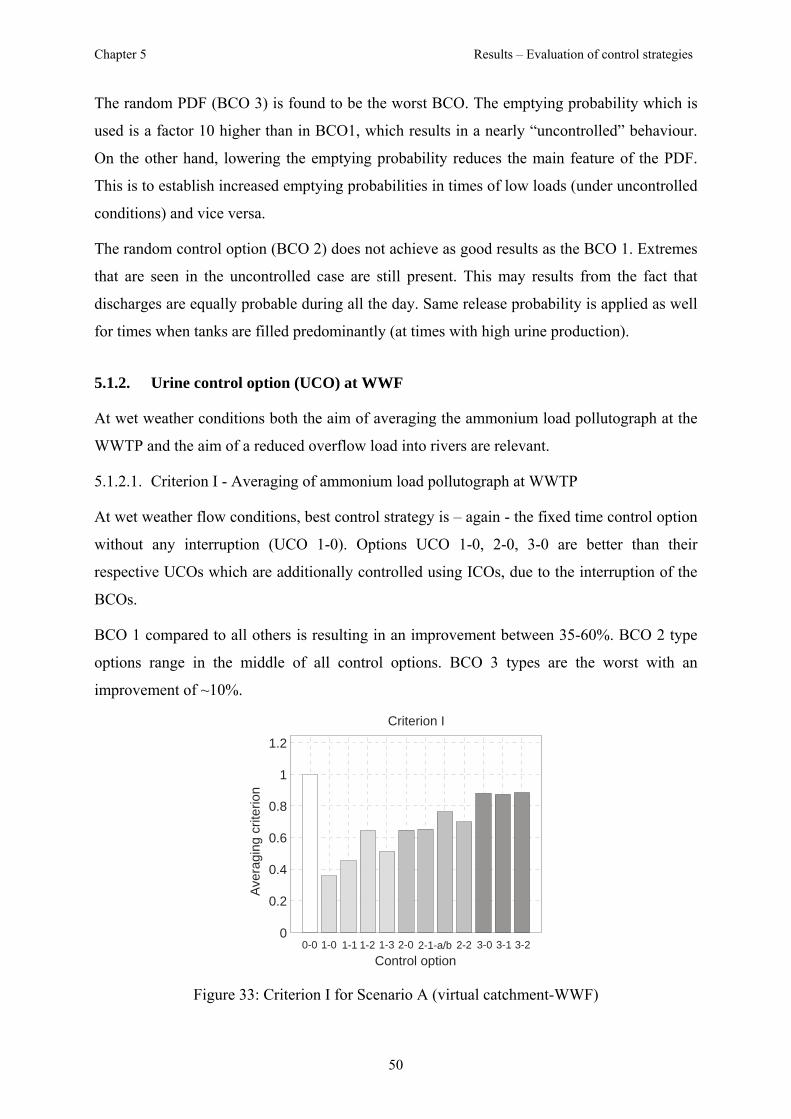
Chapter 5 Results – Evaluation of control strategies
50
The random PDF (BCO 3) is found to be the worst BCO. The emptying probability which is
used is a factor 10 higher than in BCO1, which results in a nearly “uncontrolled” behaviour.
On the other hand, lowering the emptying probability reduces the main feature of the PDF.
This is to establish increased emptying probabilities in times of low loads (under uncontrolled
conditions) and vice versa.
The random control option (BCO 2) does not achieve as good results as the BCO 1. Extremes
that are seen in the uncontrolled case are still present. This may results from the fact that
discharges are equally probable during all the day. Same release probability is applied as well
for times when tanks are filled predominantly (at times with high urine production).
5.1.2. Urine control option (UCO) at WWF
At wet weather conditions both the aim of averaging the ammonium load pollutograph at the
WWTP and the aim of a reduced overflow load into rivers are relevant.
5.1.2.1. Criterion I - Averaging of ammonium load pollutograph at WWTP
At wet weather flow conditions, best control strategy is – again - the fixed time control option
without any interruption (UCO 1-0). Options UCO 1-0, 2-0, 3-0 are better than their
respective UCOs which are additionally controlled using ICOs, due to the interruption of the
BCOs.
BCO 1 compared to all others is resulting in an improvement between 35-60%. BCO 2 type
options range in the middle of all control options. BCO 3 types are the worst with an
improvement of ~10%.
Aver
agin
g cr
iterio
n
0
0.2
0.4
0.6
0.8
1
1.2
Criterion I
Control option0-0 1-0 1-1 1-2 1-3 2-0 2-1-a/b 2-2 3-0 3-1 3-2
Figure 33: Criterion I for Scenario A (virtual catchment-WWF)

Chapter 5 Results – Evaluation of control strategies
51
5.1.2.2. Criterion II - Reduced ammonium overflow load at CSO
The fixed time emptying control with an interception that depends on rainfall (UCO 1-2)
seems to be best with regard to criterion II. An improvement of 22% is gained compared to
the baseline scenario (0-0). Lowest improvement is again observed by BCO 3 types, which
are based on random emptying in connection with a PDF. Finally BCO 2 types range in
between.
0
0.2
0.4
0.6
0.8
1
1.2
Criterion II
Control option
Emiss
ion
crite
rion
0-0 1-0 1-1 1-2 1-3 2-0 2-1-a/b 2-2 3-0 3-1 3-2
Figure 34: Criterion II for Scenario A (virtual catchment, WWF)
All in common is that options which are subjected to an additional ICO – as expected (and
intended) - have better performance regarding pollutant overflow loads. Largest improvement
is gained by option 1-2 with a relative improvement of ~25% compared with the baseline
scenario.

Chapter 5 Results – Evaluation of control strategies
52
5.1.3. Choosing best control strategy (Combination of CR1 and CR2)
The uniformly weighted criterion combines both, the aim for a averaging load at the treatment
plant inflow and a reduction of ammonium overflow load from CSOs. As earlier outlined,
criterion I (averaging) and criterion II (emission criterion) are combined as mean value of
both, applying equal weight for both.
0-0 1-0 1-1 1-2 1-3 2-0 2-1-a/b 2-2 3-0 3-1 3-2Control optionControl option
0-0 1-0 1-1 1-2 1-3 2-0 2-1-a/b 2-2 3-0 3-1 3-20
0.2
0.4
0.6
0.8
1
1.2
Criterion I+II
Figure 35: Criterion I+II (uniform weighted) for scenario A (virtual catchment, WWF)
Fixed time control options are reaching the best results. The results of random and random
PDF control options don’t comply with the expectations.
UCO 1-i are in the same range. UCO 1-2 needs a measuring equipment to gauge the
maximum effluent flow (QDR) at a CSO. UCO 1-0 is only levelling out the ammonium load
pollutograph at the WWTP inflow, no interceptive control is used. UCO 1-1 is to favour,
because UCO 1-1 causes low installation costs (it require only rain measurement) and reduces
overflow loads unlike UCO 1-0.
The implementation of a sewer system by means of urine separation will take a long time.
The time depends on the “life expectancy” of a toilet. Thus, the fixed time control with an
interruption that depends on rainfall (UCO 1-1) – the best of control – is evaluated at different
upgraded times to estimated how many years it will takes to reach a wanted result.

Chapter 5 Results – Evaluation of control strategies
53
Figure 36 shows that both, the emission based criterion (criterion II) and the averaging
criterion (criterion I) are nearly proportional to the percentage of separation toilets.
SINGLE CATCHMENT
0 0.25 0.5 0.75 10
0.2
0.4
0.6
0.8
1
Percentage of separation toilets
Crit
erio
ns
Criterion ICriterion II
UCO 1-1 (fixed time control)Stepwise implementation
Figure 36: Efficiency of control strategy UCO1-1 vs. degree of implementation

Chapter 5 Results – Evaluation of control strategies
54
5.2. TEST SCENARIO B - CASE STUDY VILS
The proposed basic control options (BCO) with associated interceptive control options (ICO)
are as well tested and evaluated using scenario B - catchment Vils Reutte. The testing is done
for a dry weather (DWF) and wet weather (WWF) conditions as described later in this
chapter.
5.2.1. Base control options (BCO) at DWF
At DWF conditions a more averaging load at the WWTP of ammonium is aimed.
Consequently criterion I is applied exclusively for evaluation.
The results are similar to the ones obtained using scenario A (virtual catchment).
Pollutographs which are generated are generally smoother than the ones obtained for the
virtual catchment. The amplitudes of the overtones on the ammonium load pollutograph are
decreased compared with the virtual catchment conditions. Reasons may be the larger
catchment (39,000 PE) which is used.
0-0 1-0 2-0 3-00
0.2
0.4
0.6
0.8
1
1.2
Criterion I
Control option
Aver
agin
g cr
iterio
n
0 6 12 18 240
200
400
600
800
Ammonium load pollutograph
t [h]
Load
[g/m
3]
NoneFixed timeRandomRandom PDF
Figure 37: Criterion of averaging; ammonium pollutograph (DWF, case study Vils)
Figure 37 shows results for criterion I (averaging) for each UCO. The averaging using the
fixed time control (UCO 1-0) is reduced down to ~20% of the baseline scenario. Second best
option is the UCO 2-0 decreasing to ~50% of the original. Only ~15% reduction is observed
for UCO 3-0 which produces a – visually – nearly equal daily variation.

Chapter 5 Results – Evaluation of control strategies
55
5.2.2. Urine control option (UCO) at WWF
5.2.2.1. Criterion I at WWF
The results of criterion I (averaging) are similar to the results from scenario A - virtual
catchment. Distribution for preferential and non preferential options is alike, where reductions
obtained are somewhat larger.
At wet weather flow conditions, the best control strategy is the fixed time control option
without an interruption (UCO 1-0). The random control options (UCO 2.i) are nearly at the
same level as UCOs 1-1, 1-2 and 1-3.
0
0.2
0.4
0.6
0.8
1
1.2
Criterion I
Control option
Aver
agin
g cr
iterio
n
0-0 1-0 1-1 1-2 1-3 2-0 2-1-a/b 2-2 3-0 3-1 3-2
Figure 38: Averaging of ammonium load pollutograph at WWTP (WWF)
5.2.2.2. Emission based criterion (criterion II)
Criterion II represents the reduction of ammonium overflow load at CSOs.
Again, results are similar to the results from scenario A - virtual catchment, having somewhat
larger reductions than in the virtual catchment.
Best result is obtained by UCO 1-1. The reductions gained by random control options (UCO
2-i) are in the same range of UCO 1-i or less than UCO 1-i.

Chapter 5 Results – Evaluation of control strategies
56
The total ammonium overflow load of the baseline scenario accounts for ~3,700 kg-NH4. The
total ammonium overflow load using UCO 1-1 accounts for ~1,570 kg-NH4. About 42% less
ammonium is spilled than without control.
0
0.2
0.4
0.6
0.8
1
1.2
Criterion II
Control option
Emiss
ion
crite
rion
0-0 1-0 1-1 1-2 1-3 2-0 2-1-a/b 2-2 3-0 3-1 3-2
Figure 39: Evaluation of UCO regarding criterion II
5.2.2.3. Immission based criterion (criterion III)
The immission based criterion (criterion III) indicates the influence of pollution in rivers.
Criterion III is – in contrast to criterion II – evaluating concentrations instead of event based
loads. Further, not combined evaluation of more locations is performed. Therefore,
criterion III was evaluated for four different points in the river system. Points considered are
shown in Figure 40:

Chapter 5 Results – Evaluation of control strategies
57
o Point I12: Lech before low flow stretch
o Point I341: Vils, before WWTP
o Point I342: Vils, after WWTP
o Point I45: Lech, before hydropower station
Figure 40: Evaluation points of CR III
Comparison of criterion II (emission criterion) and criterion III (immission criterion)
demonstrates the similar tendency with regard to the different control strategies which are
tested. In Figure 41 criterions II and III are shown, next to the temporal variation of
concentrations in the baseline scenario. Points prior the WWTP show that an increase in
concentration is observed. For river Lech this increase is less due to the larger flow - and
therefore a larger dilution - in the river. Downstream of the WWTP larger concentrations are
observed. Fluctuations in the time series are attributable to the limited abilities of the WWTP.
The WWTP in the model is considered as “perfect” treatment plant. Concentrations are
reduced such, that emission criterions (outflow limit concentrations and degree of treatment)
are fulfilled. Depending on the inflow, this scheme – where data is fed through directly and
not buffered - causes fluctuations in the concentrations.
As seen, reductions which are visual in the river are not as large as observed in criterions I
and II. This is attributable to the dilution in river having background concentrations of 0.02
and 0.016 gNH4/m³. Still, evaluations based on criterion I and II meet the outcome to
evaluations by criterion III.
In Figure 41 the concentrations temporal increase at I 342 and I 45 caused by temporal
decrease of the river flows.

Chapter 5 Results – Evaluation of control strategies
58
1.9 2 2.1 2.2 2.3 2.40
0.1
0.2
1.9 2 2.1 2.2 2.3 2.4x 10⁷
0
0.1
0.2
C [g
/m3]
1.9 2 2.1 2.2 2.3 2.4x 10⁷
0
0.1
0.2
0.3
1.9 2 2.1 2.2 2.3 2.4x 10⁷
0
0.1
0.2
I 341 - VILS, before WWTP
I 342 - VILS, after WWTP
I 12 - LECH, before low flow stretch
I 45 - VILS/LECH, before hydropower station
C [g
/m3]
C [g
/m3]
0.3
0.3
C [g
/m3]
0
0.2
0.4
0.6
0.8
1
1.2Criterion III - I341
0-0 1-0 1-1 1-2 1-3 2-0 2-1-a/b 2-2 3-0 3-1 3-2
time
x 107
0
0.2
0.4
0.6
0.8
1
1.2Criterion III - I342
0-0 1-0 1-1 1-2 1-3 2-0 2-1-a/b 2-2 3-0 3-1 3-2
0
0.2
0.4
0.6
0.8
1
1.2Criterion III - I12
0-0 1-0 1-1 1-2 1-3 2-0 2-1-a/b 2-2 3-0 3-1 3-2
0
0.2
0.4
0.6
0.8
1
1.2Criterion III - I45
0-0 1-0 1-1 1-2 1-3 2-0 2-1-a/b 2-2 3-0 3-1 3-2
Ammonium pollutopragh over evaluation period (Scenarion B - case study Vils / UCO 0-0)
Criterion III for diff. locations
0
0.2
0.4
0.6
0.8
1
1.2
Em
issi
on c
riter
ion
0-0 1-0 1-1 1-2 1-3 2-0 2-1-a/b 2-2 3-0 3-1 3-2
Emission based evaluation of urine control options (UCO)
Criterion II
CR III
CR II
COMPARISON OF CRITERION II and III
Rai
n
1.9 2 2.1 2.2 2.3 2.4x 10⁷
time
time
time
time
Figure 41: Comparison of immission and emission based criterion
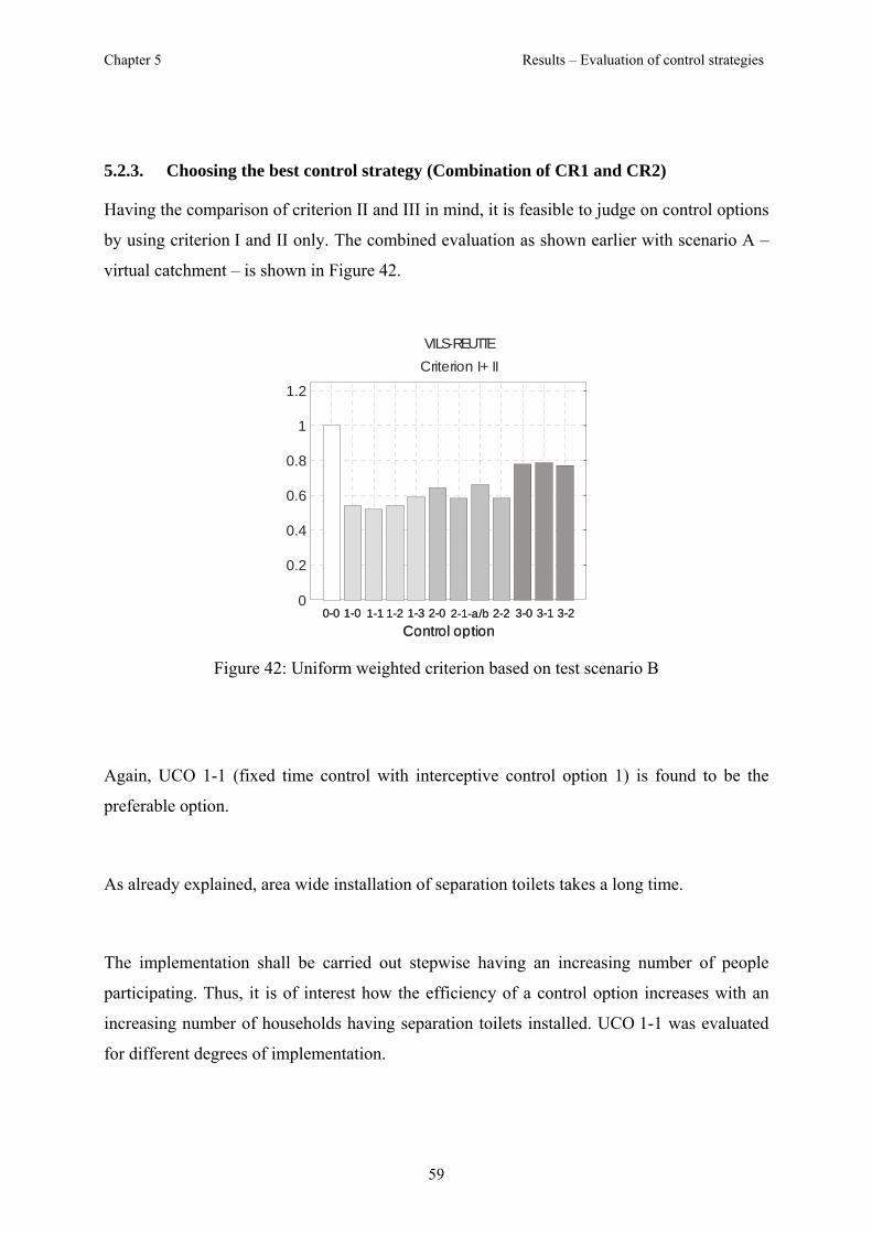
Chapter 5 Results – Evaluation of control strategies
59
5.2.3. Choosing the best control strategy (Combination of CR1 and CR2)
Having the comparison of criterion II and III in mind, it is feasible to judge on control options
by using criterion I and II only. The combined evaluation as shown earlier with scenario A –
virtual catchment – is shown in Figure 42.
0
0.2
0.4
0.6
0.8
1
1.2
Criterion I+ II
0-0 1-0 1-1 1-2 1-3 2-0 2-1-a/b 2-2 3-0 3-1 3-2Control optionControl option
0-0 1-0 1-1 1-2 1-3 2-0 2-1-a/b 2-2 3-0 3-1 3-2
VILS-REUTTE
Figure 42: Uniform weighted criterion based on test scenario B
Again, UCO 1-1 (fixed time control with interceptive control option 1) is found to be the
preferable option.
As already explained, area wide installation of separation toilets takes a long time.
The implementation shall be carried out stepwise having an increasing number of people
participating. Thus, it is of interest how the efficiency of a control option increases with an
increasing number of households having separation toilets installed. UCO 1-1 was evaluated
for different degrees of implementation.

Chapter 5 Results – Evaluation of control strategies
60
For both, the emission based criterion (criterion II) and the averaging (criterion I) are steady
decreasing if an increasing percentage of separation toilets is observed.
VILS-REUTTE
0 0.25 0.5 0.75 10
0.2
0.4
0.6
0.8
1
UCO 1-1 (fixed time control)Stepwise implementation
Percentage of separation toilets
Crit
erio
ns
Criterion ICriterion II
Figure 43: Efficiency of control strategy UCO1-1 vs. degree of implementation

Chapter 5 Results – Evaluation of control strategies
61
5.3. COMPARISON OF CONTROL STRATEGIES AT SCENARIOS A AND B
The results of criterion 1 (averaging) using the control options based on test scenario B case
study Vils are likewise the results based on test scenario A virtual catchment, but the results
are on a lower level. This is caused by the fact that the ratio - ammonium load caused by rain,
which is drained by sewer pipes / dry weather ammonium load - at case study Vils (scenario
B) is less than the ratio tested on scenario B.
Also the results of the criterion 2 (emission criterion) based on the test scenario B are less
than the results of criterion 2 tested on scenario A. The control strategy 1-2 (fixed time /
interruption depends on QDR) is much more efficient at test scenario A (virtual catchment),
because the flow time between sub catchment and combined sewer overflow (CSO) is short.
Thus the flow retention in the sewer system takes less effects regarding to the maximum
effluent flow (QDR) at a CSO.
0
0.2
0.4
0.6
0.8
1
1.2
Criterion II
Control option
Emiss
ion
crite
rion
0-0 1-0 1-1 1-2 1-3 2-0 2-1-a/b 2-2 3-0 3-1 3-2
Scenario A – virtual catchment
0
0.2
0.4
0.6
0.8
1
1.2
Criterion II
Control option
Emiss
ion
crite
rion
0-0 1-0 1-1 1-2 1-3 2-0 2-1-a/b 2-2 3-0 3-1 3-2
Scenario B – catchment Vils Reutte
Figure 44: Comparison of criterions II for scenarios A and scenario B
Chapter 5 Results – Evaluation of control strategies
62
5.4. ECONOMICAL CONSIDERATIONS
In this chapter the costs for the implementation of separation toilets in the catchment Vils are
estimated. Based on the case study Vils costs for the implementation of a urine separation
system are estimated using three different cost models.
- Amortization model (including depreciation costs)
- Initial construction model
- Support model
Based on the amortization model, the depreciation costs are the total costs of implementation.
Based on the initial construction model the costs of installing each separation toilet only one
time are included. The costs of installing each separation toilet more than one time are not
included. These costs will be paid by the population.
The 3rd calculation type is based on a support model. Costs for population are not included.
Only the amortization model calculates total costs. The initial construction model and the
support model calculate costs for the operating company. Costs for population are not
included.
Having three cost models available illustrates another novel issue of the measure.
An amortization period of 40 years is assumed as basis for the calculation. Consequently, a 40
years period is considered as maximum possible time for implementation.
Particularly description of the different financing methods is provided in the following
sections.

Chapter 5 Results – Evaluation of control strategies
63
5.4.1. Calculation of depreciation implementation costs
The calculation of the implementation costs of a sustainable waste water treatment by means
of urine separation is based on following boundary conditions:
o amortization period of 40 years (start time 2005)
o implementation period of 20 years (until all toilets in the case study are equipped with
separation toilets)
o operating life of a toilet (either conventional or separation toilets) is 10 years
o All toilets in the catchment Vils Reutte will be adapted. (22,600 separation toilets +
toilets which have to be renewed periodically, because the operating life ends after 10
years. Thus, beyond 10 years the number of separation toilets is doubled to
compensate the already installed toilets that have to be removed as well.)
o Only the additional costs arising for separation toilets are considered. Thus, only the
price difference between separation toilets (700 EUR today) and conventional toilets
(350 EUR) are considered. The costs for separation toilets are assumed to drop from
700 EUR today to 580 EUR after 40 years (without inflation). Between the 20th year
and 40th year, costs are considered stable at 580 EUR.
o Total number of toilets in the case study Vils to be constant (22,600 units)
o The yearly inflation rate is taken to be 0.02 [-]
In Table A 5 the additional costs to the conventional system are calculated with an amount of
31.2 million Euros by means of a depreciation.

Chapter 5 Results – Evaluation of control strategies
64
5.4.2. Costs of initial construction
The costs of construction are calculated in Table A 6. Assumption is
o implementation period of 20 years
o all toilets will be adapted (22,600 separation toilets)
o Only the price difference between separation toilets (700 EUR today) and
conventional toilets (350 EUR) are considered. The costs for separation toilets are
assumed to drop from 700 EUR today to 610 EUR after 20 years (instead of 40 years
in 0, without inflation).
o inflation rate of 0.02 [-]
o Costs for population are not included.
Accordingly, the construction costs amount 8.3 million Euros.
5.4.3. Costs of implementation based on a support model
To realize the implementation a support concept is postulated and costs for the supporting
institution (e.g. the AWV-Vils) are calculated. Assumption is that the support rate granted by
the municipality rises stepwise until 75% of toilets are implemented as separation toilets.
Progressive people are open to use new technology although only little support rates are
granted. Others, also people which are interested in new technology will use it if somewhat
higher support rates are granted. The remaining population is only convincible in case the
technology is already state of the art. Based on this assumption, the support rates are
increased stepwise for different levels of implementation.
Table 9: Rates of support model Upgrade Support rate People 0 - 25% 0.20 progressive
25 - 50% 0.35 more interested 50 - 75% 0.50 interested 75 - 100% 0.00 others
Based on the case study Vils, an inflation rate of 0.02 and the assumption that all toilets in the
catchment will be adapted (22,600 separation toilets), the support costs are calculated in Table
A 7 and amount 4.6 million Euros. Costs for population are not included.

Chapter 6 Summary and Conclusions
65
5.4.4. Comparison of implementation costs
In Figure 45 the cumulative costs over the time of each implementation are plotted.
0 10 20 30 390
5
10
15
20
25
30
35x 106 Implementation costs
time [a]
EUR
(cum
ulat
ive)
Amortization model (total costs)Initial construction model (costs for operating company)Support model (costs for operating company)
Figure 45: Comparison of implementation costs
If the waste water treatment by means of urine separation is financed according to the cost
model “initial construction” or the cost model “support”, the costs will be competitive, but the
costs for population are not included. This is not only true for final cumulated costs, but as
well during the implementation period.
Annual costs per person
To qualify the costs, annual costs per person are calculated, based on an operating time of 40
years. Costs are distributed between all inhabitants (38,000 PE). Thus, it can be seen that
implementation of a separation system does not cost a fortune.
Table 10: Cumulative costs of different implementations Costs EUR/PE/a Depreciation costs 20.51 Total costs Construction costs 5.44 Costs for operating company Supporting costs 3.05 Costs for operating company

Chapter 6 Summary and Conclusions
66
6. SUMMARY AND CONCLUSIONS
In this chapter the work with CITY DRAIN, the used urine control options and the
economical considerations are reflected.
CITY DRAIN was used because one advantage of the software is the flexibility regarding the
implementation of new features. The CITY DRAIN library can be added with new blocks
from the Simulink library and with new programmed blocks. The program language is easily
to understand, thus the learning period will be short. Another advantage is the block based
modelling of urban waste water treatment systems, because the block formation in the model
regards with the formation of structures in the plan.
Considering the inherent uncertainties within the Vils-Reutte catchment, the obtained
calibration quality is “as accurate as possible”. Thus the actualities of situation are reflected
and the performance of the tested urine control strategies based on the case study Vils Reutte
could be evaluated, adequately.
The urine separation in connection with controlled urine tank emptying is an efficient strategy
to reach both goals:
1) averaging the ammonium load pollutograph
The ratio maximum / minimum ammonium overflow load changed from ca. 2 to 1.1.
2) reduce ammonium concentration peaks in rivers.
About 42% less ammonium is spilled into rivers than without control.
The reduction of the ammonium concentrations in rivers amounts about 10-15%.
The performance indicators for each goal
- averaging criterion
- emission based crtierion
- and immission based criterion
were hardly to define. In conclusion the emission based criterion was assigned as an indicator
for loads and the “immission” criterion – which serves as crosscheck of criterion I and II – for
concentrations.
The fixed time control in connection with interceptive control option 1 (depends only on
rainfall) is the best control strategy, because the results of the performance indicators are good

Chapter 7 Literature
67
and the implementation costs of this strategy are less than the costs of the fixed time control
in connection with interceptive control option 2 or 3, due to the interceptive controls that
depend on forecast or sewer data need a central station in any case.
An improvement of the best control strategy will be possible, if the fixed time control option
is not based on an equidistant emptying pattern. In times with high ammonium load peaks at
the treatment plant, more urine tank emptyings should be executed as in times with an average
ammonium load level.
The economic considerations are difficult to estimate, but the different cost models show the
order of magnitude.

Chapter 7 Literature
68
7. LITERATURE
Achleitner S., Möderl M. und Rauch W. (2006). CITY DRAIN © - an open source approach for simulation of
integrated urban drainage systems.
Achleitner S., De Toffol S., Engelhard C. und Rauch W. (2005). Model based hydropower gate operation for
mitigation of CSO impacts by means of river base flow increase. Wat.Sci.Tech, 52 (5),87-94.
Berndtsson J. C. (2005). Experiences from the implementation of a urine separation system: Goals, planning,
reality. Building and Environment, 41 (4),427-437.
Brombach H. und Fuchs S. (2003). Datenpool gemessener Verschmutzungskonzentrationen in Misch- und
Trennkanalisationen. KA - Abwasser, Abfall, 50 (4),441-450.
DeToffol S. und Rauch W. (2006). Combined systems versus separate systems - an assessment of ecological and
economical performance indicators. 7th International Conference on Urban Drainage Modelling and
the 4th International Conference on Water Sensitive Urban Design, Melbourne, Australia. 2-7 April
2006.
Grecu M. und Krajewski W. F. (2000). A large-sample investigation of statistical procedures for radar-based
short-term quantitative precipitation forecasting. Journal of Hydrology, 239 (1-4),69-84.
Hanæus J., Hellström D. und Johansson E. (1997). A study of a urine separation system in an ecological village
in Northern Sweden. Water Science and Technology, 35 (9),153-160.
Jönsson H., Stenström T.-A., Svensson J. und Sundin A. (1997). Source separated urine-nutrient and heavy-
metal content, water saving and faecal contamination. Water Science Technology, 35 (9),145-152.
Kvarnström E. und Stintzing A. R. (2005). Swedish farmers attitudes to reuse of digestion residues from
anaerobic digestion and sourcediverted urine. 3rd International Conference on Ecological Sanitation,
Durban, South Africa. 23 - 26 May 2005.
http://conference2005.ecosan.org/papers/kvarnstrom_et_al.pdf.
Larsen T. A. und Gujer W. (1996). Separate management of anthropogenic nutrient solutions. Water Science
Technology, 34 (3-4),87-94.
Lautrich R. (1980). Der Abwasserkanal. Handbuch für Planung, Ausführung und Betrieb., Parey, Hamburg,
OEWAV R19 (Draft 2003). OEWAV- Regelblatt 19: Richtlinien für die Bemessung and Gestaltung von
Regenentlastungen in Mischwasserkanaelen. Oesterreichischer Wasser- und Abfallwirschaftsverband,
Vienna, Austria.
OEWAV (2001). Benchmarking in der Siedlungswasserwirtschaft.
OEWWV R11 (1982). Richtlinien für die abwassertechnische Berechnung von Schmutz-, Regen- und
Mischwasserkanälen .
Otterpohl R., Braun U. und Oldenburg M. (2002). Innovative Technologies for Decentralised Wastewater
Management in Urban and Peri-Urban Areas. 5th Specialised Conference on Small Water and
Wastewater Treatment Systems, Istanbul-Turkey, 24-26 September 2002.
http://www2.gtz.de/ecosan/download/iwa2002-otterpohl.pdf.
Rauch W., Brockmann D., Peters I., Larsen T. A. und Gujer W. (2003). Combining urine separation with waste
design: An analysis using a stochastic model for urine production. Water Research, 37 (3),681-689.

ANNEX
1
ANNEX
Table A 1: Calibrated data of sewers between sub catchments ID l [m] tf [min] ID l [m] tf [min] ID l [m] tf [min]
0-1 1200 16 8 1579 20 18 572 3
0-2 1800 35 9 281 4 19 2590 42
0-3 1400 30 10 1835 21 20 961 15
1 3169 40 11 496 10 21 630 8
2 1863 40 12 579 14 22 529 4
3 1453 20 13 385 10 23 1421 10
4 573 12 14 1038 16 24 277 5
5 1064 9 15 325 2 25 5257 87
6 323 3 16 762 8 26 4685 78
7 684 8 17 399 6
Table A 2: Calibrated data combined sewer overflows CSO-ID V QDR [m³] [l/s]
1 800 190
2 280 325
3 134 20
RE
UT
TE
4 270 65
5 800 80
6 374 60
7* 0 0VIL
S
8 200 80
Table A 3: Calibrated data of pumping stations PS-ID Pumping Station Sewer QP Voff Von V [m³/s] [m³] [m³] [m³]
1 Klosterweg 02 0.150 18.50 2 Rieden 08 0.008 0.40 3.27 2.87 3 Musau 09 0.011 0.22 0.92 0.70 4 Roßschläg 09 0.009 0.23 0.91 0.68 5 Oberpinswang 10-1 0.011 0.40 2.71 2.31 6 Unterpinswang 10-2 0.011 0.40 2.85 2.45 R
EU
TT
E
7 Heiterwang 12 0.0110 22.15
Shaded cells are modified.

ANNEX
2
Table A 4: Calibrated data of sub catchments Village # Catchment Type PE A tf f hv,i hv,d [ha] [min] [-] [mm] [l/(s*ha)]
Pfronten Pfronten 13105 211.6 1-1 Pfronten 1 CSS 1618 26.1 30 0.10 1 1.25 1-1-1 Pfronten 1-1 SSS 2556 41.3 30 0.10 1 1.25 1-2 Pfronten 1-2 CSS 4961 80.1 28 0.10 1 1.25V
ILS
1-3 Pfronten 1-3 CSS 3970 64.1 22 0.10 1 1.25Vils 2 Vils CSS 1731 94.5 25 0.10 1 1.25Pinswang SSS 485 19.5 3 Unterpinswang 295 11.8 33 0.19 1 1.25 4 Oberpinswang 190 7.6 20 0.20 1 1.25Musau SSS 374 23.0 5 Musau 256 15.8 29 0.18 1 1.25 6 Brandstatt 90 5.5 12 0.19 1 1.25 7 Roßschläg 28 1.7 3 0.21 1 1.25Pflach SSS 1277 59.4 8 Pflach O 781 36.3 28 0.18 1 1.25 9 Pflach W 496 23.1 31 0.16 1 1.25Reutte CSS 8289 187.5 10 Reutte N 3195 72.3 24 0.15 0.8 1.25 11 Reutte SW 2959 66.9 29 0.15 0.8 1.25 12 Reutte SO 2135 48.3 30 0.15 0.8 1.25Breitenwang 2728 101.1 13 Breitenwang CSS 814 30.2 33 0.15 0.8 1.25 14 Mühl SSS 1619 60.0 40 0.16 1 1.25 15 Lähn P CSS 150 5.5 7 0.15 0.8 1.25 16 Lähn L CSS 146 5.4 4 0.15 0.8 1.25Lechaschau 2148 79.9 17-1 Nord SSS 967 36.0 21 0.19 1 1.25 17-2 Süd SSS 1181 44.0 23 0.19 1 1.25Wängle 1394 35.2 18 Wängle CSS 1355 34.2 19 0.15 0.8 1.25 19 Holz CSS 39 1.0 6 0.21 1 1.25Ehenbichl 1521 31.1 20 Ehenbichl SSS 1138 23.3 20 0.18 1 1.25 21 Rieden SSS 383 7.8 14 0.23 1 1.25Höfen 1756 66.3 22 Höfen NW SSS 481 18.2 9 0.16 1 1.25 23 Höfen NO SSS 715 27.0 28 0.16 1 1.25 24 Höfen S SSS 560 21.1 15 0.19 1 1.25
RE
UT
TE
Weissenbach 25 Weissenbach SSS 1588 52.8 55 0.21 1 1.25 Heiterwang 26 Heiterwang SSS 707 27.6 24 0.18 1 1.25 Bichelbach 27 Bichelbach SSS 1264 5.0 6 0.18 1 1.3
Shaded cells are modified.

ANNEX
3
Table A 5: Calculation of implementation costs based on a depreciation Year Toilets Price/Separation
Toilet Price/Separation
Toilet Price/Conventional
Toilet Costs
present [EUR]
future [EUR]
future [EUR]
future [EUR]
0 1130 700 700 350 3954801 1130 700 714 357 4033902 1130 700 728 364 4114583 1130 700 743 371 4196874 1130 700 758 379 4280815 1130 670 740 386 3992166 1130 670 755 394 4072007 1130 670 770 402 4153448 1130 670 785 410 4236519 1130 670 801 418 432124
10 2260 640 780 427 79888911 2260 640 796 435 81486712 2260 640 812 444 83116413 2260 640 828 453 84778714 2260 640 844 462 86474315 2260 610 821 471 79079316 2260 610 837 480 80660917 2260 610 854 490 82274118 2260 610 871 500 83919619 2260 610 889 510 85597920 2260 580 862 520 77235721 2260 580 879 530 78780422 2260 580 897 541 80356023 2260 580 915 552 81963124 2260 580 933 563 83602425 2260 580 952 574 85274426 2260 580 971 586 86979927 2260 580 990 597 88719528 2260 580 1010 609 90493929 2260 580 1030 622 92303830 2260 580 1051 634 94149931 2260 580 1072 647 96032932 2260 580 1093 660 97953533 2260 580 1115 673 99912634 2260 580 1137 686 101910835 2260 580 1160 700 103949136 2260 580 1183 714 106028037 2260 580 1207 728 108148638 2260 580 1231 743 110311639 2260 580 1256 758 1125178
31174636

ANNEX
4
Table A 6: Construction costs of implementation Year Toilets Price/Separation
Toilet Price/Separation
Toilet Support rate Costs
present [EUR] future [EUR] EUR 0 1130 700 700 350 3954801 1130 700 714 357 4033902 1130 700 728 364 4114583 1130 700 743 371 4196874 1130 700 758 379 4280815 1130 670 740 386 3992166 1130 670 755 394 4072007 1130 670 770 402 4153448 1130 670 785 410 4236519 1130 670 801 418 432124
10 1130 640 780 427 39944411 1130 640 796 435 40743312 1130 640 812 444 41558213 1130 640 828 453 42389414 1130 640 844 462 43237215 1130 610 821 471 39539616 1130 610 837 480 40330417 1130 610 854 490 41137018 1130 610 871 500 41959819 1130 610 889 510 427990
22599 8272013
Table A 7: Support model cost of implementation Year Toilets Price/Separation
ToiletPrice/Separation
ToiletSupport
rate Costs
present [EUR] future [EUR] EUR 0 1130 700 700 0.2 1581921 1130 700 714 0.2 1613562 1130 700 728 0.2 1645833 1130 700 743 0.2 1678754 1130 700 758 0.2 1712325 1130 670 740 0.35 2925506 1130 670 755 0.35 2984017 1130 670 770 0.35 3043698 1130 670 785 0.35 3104579 1130 670 801 0.35 316666
10 1130 640 780 0.50 44076611 1130 640 796 0.50 44958212 1130 640 812 0.50 45857313 1130 640 828 0.50 46774514 1130 640 844 0.50 47710015 1130 610 821 0.00 016 1130 610 837 0.00 017 1130 610 854 0.00 018 1130 610 871 0.00 019 1130 610 889 0.00 0
22599 4639447

ANNEX
5
VERPFLICHTUNGSERKLÄRUNG
Ich erkläre, dass ich meine Diplomarbeit selbständig verfasst habe und alle in ihr verwendeten
Unterlagen, Hilfsmittel und die zugrundegelegte Literatur genannt habe.
Ich nehme zur Kenntnis, dass auch bei auszugsweiser Veröffentlichung meiner Diplomarbeit
das Institut, an dem die Diplomarbeit ausgearbeitet wurde, und der Betreuer zu nennen sind.
Innsbruck, am