molecular mechanisms of salt effects on carbon …6,5) of 4.067 nm long solvated in pure nmp...

Supporting information to:

Molecular mechanisms of salt effects on carbon nanotube dispersions in an organic solvent (N-methyl-2-pyrrolidone)

Andrey I. Frolov, Raz N. Arif, Martin Kolar, Anastasia O. Romanova, Maxim V. Fedorov*,

Aleksey G. Rozhin*

Table of Content:

1. Simulation details

2. Comparison of water and NMP radial density profiles around CNT

3. Details on the calculation of the preferential interaction coefficient

4. Details of experimental results

5. Effect of concentration on the preferential interaction coefficient: simulation of the

CNT(8,6) dissolved in 0.01M NaI solution in NMP

* Corresponding authors: [email protected], [email protected] (MVF), [email protected] (AGR)

Electronic Supplementary Material (ESI) for Chemical ScienceThis journal is © The Royal Society of Chemistry 2011

Part 1. Simulation details for the systems: a segment of CNT dissolved in 0.15M NaI

solution in NMP.

1) Systems under the investigation.

We performed Molecular Dynamics (MD) simulations using the Gromacs 4.5 MD software

package.1 We simulated a segment of CNT (8,6) of 5.186 nm long and a segment of CNT

(6,5) of 4.067 nm long solvated in pure NMP (N-methyl-2-pyrrolidone) and 0.15M NaI NMP

solution. Additionally we performed simulations of the bulk NMP solvent.

2) Molecular topology and potential parameters used in the simulations.

Firstly, we generated a molecular simulation topology for a CNT segment consisted of 592

carbon atoms (chirality (8,6) with tubule radius of 0.477 nm) and a CNT segment consisted of

364 carbon atoms (chirality (6,5) with tubule radius of 0.377 nm). For generation of the CNT

topologies we used the on-line TubeGen 3.3 tool.2 Then the CNT(8.6) and the CNT(6,5) were

placed in a rectangular simulation box of the size 7.50×7.50×5.19 nm3 and 7.25×7.25×4.07

nm3 correspondingly. The CNT segments were oriented along the Z axis of the boxes. We

used the rectangular periodic boundary conditions, where the CNT was treated as a “periodic

molecule”. The positions of the CNT atoms were restrained to the initial values by harmonic

potential with 1000 kJ mol-1 nm-2 force constant in each direction.

The Gromacs topology input files for the CNTs were generated by the x2top program that is

a part of the Gromacs 4.5 suite. We used the short-range Lennard-Jones nonbonded

interaction parameters for the CNT carbon atoms that corresponded to the benzene OPLS-AA

(all-atom optimized molecular potential for liquid simulation)3 carbon (opls_145 in the

Gromacs notation). However, the partial charges of the CNT carbons were set to zero. The

equilibrium values for the structural parameters of the bonded interactions (bond lengths,


angles) were taken from the initially generated structure of CNT, while the force constants for

the bond and angle harmonic potentials were adopted from the OPLS-AA force field.3 The

absence of dihedral potentials is compensated by the restraining potential. The non-bonded

interactions in the systems were pair-wise additive. The Lennard-Jones coefficients for atoms

of different kinds were obtained as a geometric mean value of the parameters of two

corresponding particles:

ij ii jj

ij ii jj

ε ε ε

σ σ σ

= ⋅

= ⋅, (S 1)

where i and j indicate type of particle.

The OPLS-AA potential parameters were assigned to NMP molecule with the use of

Shrodinger Maestro software.4 The parameters were then transformed into the Gromacs

topology format, where the Fourier coefficients of the dihedral potential term were

transformed into the Ryckaerd-Bellemans type.5 The OPLS-AA parameters were already

verified by the previous simulation study.6 We used the sodium and iodide ion potential

parameters developed by Jensen and Jorgensen.7 However, to prevent possible crystallization

of the salt during the simulation time we increased the interionic Na I

σ + −− Lennard-Jones term,

estimated by Equation (S 1) by 0.05 nm.

3) MD algorithms details.

We used the leap-frog integrator with 0.002 ps integration time step. For the Lennard-Jones

potential we used 1.00 nm cut-off radius with shifting potential method. The neighbor list for

the nonbonded interactions was updated each 10th integration step. For accurate evaluation of

the long range Coulomb interactions we used the Particle Mesh Ewald method8 with 1.10 nm


cut-off radius for the real space sum and 0.12 nm spacing for the mesh in the real space. The

cubic B-splines were used to map the charges on the mesh.

The length of all the bonds with hydrogen atoms were fixed to the force field equilibrium

values by the LINCS algorithm.9

For the NVT-ensemble (canonical ensemble) simulations we used the “v-rescale”

thermostat10 with the reference temperature of 300K and the relaxation time of 2.0 ps in the

case of “production run” and 1.0 ps in the case of “equilibration run”. For the NPT-ensemble

(isothermo-isobaric ensemble) simulations we used the Berendsen thermostat and also the

Berendsen barostat.11 In this case the system was coupled to an external pressure of 0.1013

MPa with the relaxation time of 1.0 ps.

4) Systems preparation and collection of statistics.

The segment of CNT (8,6) was solvated in 0.15M NaI NMP solution containing 1600 NMP

molecules, 27 Na+ ions and 27 I- ions. To generate the initial configuration of the molecules

we used the Packmol program.12 The configuration was then optimized by Gromacs using the

energy minimization routine. To equilibrate the density, the resulting system was simulated

during 0.2 ns of the simulation time in the NPT-ensemble. Then it was simulated in the NVT-

ensemble for 60 ns. Coordinates of the system were sampled each 0.3 ps for the further

analysis.

The segment of CNT (6,5) was solvated in 0.15M NaI NMP solution containing 1200 NMP

molecules, 19 Na+ ions and 19 I- ions. To generate the initial configuration of the molecules

we used the Packmol program.12 The configuration was then optimized by Gromacs using the

energy minimization routine. To equilibrate the density, the resulting system was simulated

during 0.2 ns of the simulation time in the NPT-ensemble. Then it was simulated in the NVT-


ensemble for 50 ns. Coordinates of the system were sampled each 0.3 ps for the further

analysis.

To enhance statistics and to estimate the errors in the calculated preferential interaction

coefficients and the free energies changes, we performed 10 replica simulations for each CNT

starting from different initial coordinates. The initial configurations for the replica runs were

collected by taking coordinates of the system each 3 ns and 5 ns from the initial simulations

for the systems with CNT(8,6) and CNT(6,5) correspondingly. Each replica was firstly

simulated for 0.2 ns at elevated temperature (450K) and then annealed to 300K during 0.1 ns

of simulation time in NVT ensemble. The production simulation times for each replica were

15.9 and 20.7 ns for systems with CNT(8,6) and CNT(6,5) correspondingly. Coordinates of

the system were sampled 0.4 ps for the replica simulations for further analysis.

The pure NMP-NaI solvent system contained 610 NMP molecules, 18 Na+ ions and 18 I-

ions that were 0.2 ns of NPT simulation. The system was simulated during 100 ns of

simulation time in NVT-ensemble.

5) Details on the calculation of radial density profiles.

The radial density profiles (RDPs) of different species were calculated from the MD

trajectory for all the replica simulations with the g_rdf program of Gromacs 4.5 suite. The

RDPs are normalized by the number density of species in the corresponding simulation box

(number of particles/total volume). We note that in the simulation there is a large excluded

volume of the CNT, which is not accessible by the solvent. Because of this, the number

density of species is underestimated by g_rdf and, consequently, although the calculated

RDPs become constant at large r values, these constants are larger than 1. To correct this

artifact we have chosen a region on each RDP where it reaches a plateau (2.5 nm < r < 3.0 nm

for the case of CNT(8,6) and 2.4 nm < r < 2.9 nm for the case of CNT(6,5). We averaged the


RDPs over this region and correspondingly rescaled the RDPs (divided by the mentioned

value). (See also the supporting information of Ref. 13). On the Figure 3 of the main text the

scaled RDPs are shown.

6) Details on the calculation of ion solvation numbers.

For the calculation of the solvation number we use the following criteria. We counted the

number of nitrogen atoms of NMP molecules within 0.73 nm and 0.50 nm from the centres of

an iodide and a sodium ions correspondingly.


Part 2. Comparison of water and NMP radial density profiles around CNT

Radial density profiles of water as a function of the distance from CNT (7,0) in aqueous

dispersion is obtained by the analysis of MD trajectories of our previous work Ref. 13 (see

Figure S1).

On Figure S1 one can see that the CNT surface is much stronger solvated in NMP,

compared to its hydration in water. In the NMP solution, there is a dense solvation shell

around CNT which is represented by a broad region on the NMP radial density profile that

consists of two distinct high peaks. The peaks are followed by a deep hollow at about

6.5CNTr r− = nm, which indicates the outer radius of the first dense NMP solvation shell

around the CNT.

Contrary, the water radial density profile has a much smaller height of the first peak and

much less deep hollow, showing that the CNT hydration shell is much more diffuse compared

to the NMP solvation shell. Thus, partial dehydration of CNT surface in water is much easier

than the partial desolvation of CNT in NMP, where the barrier is large. The barrier of a

solvent molecule exchange between the 1st solvation shell and the rest of solution is more than

1 kBT higher in the NMP solution compared to the aqueous solution (Figure S2). We note that

similar effects were observed for graphene sheets solvated in NMP and water in the Ref. 6.


Figure S1. Radial density profiles of water (TIP4Pew model)13 and NMP (OPLS-AA parameters) around the CNT(7,0) and CNT(8.6) correspondingly. One can see CNT surface much more strongly solvated in NMP, rather than hydrated in water.

Figure S2. Potential of mean force of water (TIP4Pew model)13 and NMP (OPLS-AA parameters) around a CNT. One can see a high barrier of 2.6 kBT preventing a free exchange of NMP molecules between the solvation shell of the CNT and the rest of solution. Contrary, in the aqueous solution the barrier of water exchange is only 1.5 kBT. The PMFs were estimated as negative natural logarithms of the corresponding radial density profiles.

0

( )rρρ

PMF(r-rCNT)

[kBT]


Part 3. Details on the calculation of the preferential interaction coefficient (on an

example of the system with the CNT(8,6)).

Following the methodology for the characterization of the “salting out effect” in aqueous

solutions, we have estimated the change of the CNT surface Gibbs free energy upon the salt

addition based on the Gibbs-Duhem relation (as described in Refs. 14,15) and approach based

on the Kirkwood-Buff theory of solutions16 as discussed in Refs 17–19. In the framework of the

Gibbs-Duhem theory of solution, the change in the chemical potential of a solute molecule (S)

dissolved in a solvent (V), upon addition of a co-solvent (X) is written as:14

S SX Xd dµ µ= −Γ ⋅ , (S1)

where Sdµ is the change in the chemical potential of solute, Xdµ is change of chemical

potential of the co-solvent, SXΓ is the solute - co-solvent preferential interaction coefficient

(deficit or excess of the number of co-solvent molecules around a solute molecule, compared

to the same volume of the bulk solution).

We substitute the differentials with the finite differences, and get the expression which can

be used in our calculations:

S SX Xµ µ∆ ≈ −Γ ⋅∆ , (S2)

The solute - co-solvent preferential interaction coefficient can be calculated within the

Kirkwood-Buff theory of solutions:17,20

( )2

0

, ,

SSX X SX SV

X T P n

G Gµ ρµ

⎛ ⎞∂Γ = − = −⎜ ⎟∂⎝ ⎠

, (S3)

where 0Xρ is the number density of species X, GAB is a Kirkwood-Buff (KB) integral for

species A and B.


Initially a KB integral was defined via a molecule-molecule radial distribution function

gAB(r).21 A straightforward generalization for molecule-molecule pair correlation function

(gAB(r)) defined in 3D coordinate space would be:20

( )( ) 1AB ABV

G g d= −∫ r r , (S4)

where V defines the whole “phase volume” of the r coordinate.

Because CNT (S) has spherical symmetry, we rewrite the KB integral (Equation S4) in

cylindrical coordinates through the radial density profile 0

( )AB

B

rρρ

:

00

( ) 1 2SBSB

B

rG r drρ πρ

∞ ⎛ ⎞= − ⋅⎜ ⎟

⎝ ⎠∫ , (S5)

where ( )SB rρ is the number density of particles B as a function of the distance r from the

axis of cylindrical symmetry of CNT (S), 0Bρ is the number density of B in bulk solution, the

integration is performed in cylindrical coordinates, 2 r drπ ⋅ is the volume of cylindrical

segment (the length of the cylinder is implied to be 1 nm).

Thus, for our case the preferential interaction coefficient (Equation S3) can be written as

follows:

00 0

0

( ) ( ) 2SX SVSX X

X V

r r r drρ ρρ πρ ρ

∞ ⎛ ⎞Γ = − ⋅⎜ ⎟

⎝ ⎠∫ (S6)

Following the works (Ref. 22) we applied the Kirkwood-Buff theory to estimate the

preferential interaction coefficient of the NaI salt at CNT surface. The KB theory is developed

for open systems. But in an open system, one can not consider ions of the dissociated salt as

independent components, because of the electroneutrality condition. Kusalik and Patey

described a rigorous way how to treat ionic solutions within the KB theory 23. Chitra et al. 22


showed that the results of Kusalik and Patey are equivalent to the following “physical

picture”: considering ions (both cations and anions) as “indistinguishable” particles. Thus in

this study we consider the “indistinguishable” ions as a co-solvent to NMP. Following the

work of 15 we estimated the RDP of the “indistinguishable ions“ as an arithmetic mean of the

contributions coming from the sodium and iodide RDPs:

0 0 0

( ) ( )( ) 12

SNa SISX

X Na I

r rr ρ ρρρ ρ ρ

+ −

+ −

⎛ ⎞⎜ ⎟= +⎜ ⎟⎝ ⎠

, and the bulk density of the “indistinguishable ions“ as the

sum of the number densities of Na+ and I- ions.

The preferential interaction coefficient evaluated by Equation S6 is illustrated in Figure S3.

Figure S3. The calculated preferential interaction coefficient of salt for 1 nm of the CNT(8,6) length. In this particular case, the plots were estimated over the last 30 ns trajectory. A) Integrand function in Equation S6; B) Preferential interaction coefficient as a function of distance (running integral of Equation S6). Te value of SXΓ , used in further calculations, was

set to (3.0) 0.547SXΓ = − [ion pairs / nm of CNT length].

The changes in the chemical potentials of co-solvent and solvent in the bulk solution are

related by the following Gibbs-Duhem equation:15

VX V

X

xd dx

µ µ= − ⋅ or VX V

X

xx

µ µ∆ ≈ − ⋅∆ , (S7)

where xB is the mole fraction of species B (B=X,V) in bulk solution.

Change of the chemical potential of solvent upon the co-solvent addition can be written as:15


ln( )V B Vk T aµ∆ = , (S8)

where kB is the Boltzmann constant, T is temperature, aV is the activity of the solvent.

Since in our case we have a diluted solution (0.15M), we may assume that the activity of the

solvent is equal to the mole fraction of solvent: V Va x≈ . Considering the ions as separate

species we can estimate the mole fraction of solvent: 1600

1600 27 2Vx =+ ⋅

. The change of the

chemical potential of solvent upon the co-solvent addition can be estimated:

ln( )V B Vk T xµ∆ ≈ ⋅ . Thus, following the Equation S7 ( )lnVX B V

X

xk T xx

µ∆ ≈ − ⋅ ⋅ and the final

expression is (see Eq. S1):

( )lnVS B SX V

X

xk T xx

µ∆ ≈ ⋅Γ ⋅ ⋅ (S9)

We calculated the change in the chemical potential of CNT dissolved in NMP upon addition

of sodium iodide salt for all simulation we had (10 replicas and the last 20 ns of the initial

simulation). We present the results in the Table 1 of the main text and Table S2 of the

supporting information. Note, the values calculated by the Equation S2 are then normalized

by the surface of the CNT of 1 nm length ( 2 CNTS rπ= , where the radius of CNT(8,6)

0.477 0.15CNTr = + [nm] and CNT(6,5) 0.377 0.15CNTr = + [nm], 0.15 nm being the radius of

a carbon atom).

The change in the chemical potential of CNT is positive indicating an increase of the CNT

solvophobicity upon the salt addition.

Analyzing the described expressions, we can estimate how an increase of salt

concentration would affect the thermodynamic stability of the CNT-NMP dispersions. We

rewrite the Eq. S9 as:


1 ln(1 )XS B SX X

X

xk T xx

µ −∆ ≈ ⋅Γ ⋅ ⋅ − (S10)

Assuming that the particle radial density profiles do not change too much for small salt

concentration, we may conclude that the preferential interaction coefficient (equation S6) is

proportional to the salt concentration, so SX Xconst xΓ ≈ ⋅ , where the const is negative.

Moreover, for small salt concentrations we also may assume ln(1 )Xx x− ≈ − and ( )1 1Xx− ≈ .

The combination of the above mentioned formulas gives the following relation of Sµ∆ and

the salt concentration Xx :

( )S B Xconst k T xµ∆ ≈ ⋅ ⋅ − (S11)

Taking into account the negative sign of the const , we may conclude that with an increase

of the salt concentration Sµ∆ increases (becomes more positive), thus the CNT becomes more

solvophobic.


4. Details of experimental results

Figure S4. Photographs of the samples. A) 15 minutes upon the salt addition; B) 5 hours upon the salt addition; C) samples after ultracentrifugation.

The PL spectra intensity correlates with the concentration of the dispersed (single) CNTs

and small bundle in the dispersion.24,25 However it is known that metallic CNTs efficiently

quench PL of the bundle they belong to. Due to the high probability to meet a metallic CNT in

a big bundle, it is commonly accepted that the big bundles do not contribute much to the PL

spectra of CNTs dispersions.24

Full PL data are represented in Table S1. The CNT characteristic “spots” on the PL maps

indicate the presence of the CNTs of different chiralities in the dispersion. However, at higher

concentrations of salt the remaining CNT concentration in negligible comparing to the initial

sample concentration.

The peaks on PL spectra indicate that upon the salt addition the dispersion contains CNTs

in either single dispersed or in small bundle forms. Absorption spectra confirm the results of

PL spectra. The monotonic drop of the absorption spectra intensities (Figure S6) shows that

the degree of sedimentation of the CNTs from the CNT-NMP dispersion can be regulated by

the salt concentration.


400 600 800 1000 1200 1400 16000.0

0.1

0.2

0.3

0.4

0.5

0.6 No salt C(salt) = 0.1mM C(salt) = 0.5mM C(salt) = 1mM C(salt) = 10mM

A

bsor

banc

e, a

.u.

Wavelength, nm

Figure S5. Optical absorption of the samples with different concentration of NaI salts immediately after addition of salts.

Table S1. PL spectra of the CNT-NMP-salt systems.

Concentration, mM Before centrifugation After centrifugation

0 (control)

1000 1250 1500

400

600

800

8,4

7,67,58,3

7,3

6,5

Exci

tatio

n, n

m

Emission, nm

3000450060007500900010500120001350015000

1000 1250 1500

500

750

7,3

8,4

7,67,58,3

6,5

Exci

tatio

n, n

m

Emission, nm

3000450060007500900010500120001350015000

0.1

1000 1250 1500

400

600

800

8,4

7,67,58,3

7,3

6,5

Exci

tatio

n, n

m

Emission, nm

3000450060007500900010500120001350015000

1000 1250 1500

400

600

800

7,3

8,4

7,67,58,3

6,5

Exci

tatio

n, n

m

Emission, nm

3000450060007500900010500120001350015000


0.5

1000 1250 1500

400

600

800

8,4

7,67,58,3

7,3

6,5

Exci

tatio

n, n

mEmission, nm

3000450060007500900010500120001350015000

1000 1250 1500

400

600

800

Exci

tatio

n, n

m

Emission, nm

3000450060007500900010500120001350015000

1

1000 1250 1500

400

600

800

8,4

7,67,5

7,3

8,3

6,5

Exci

tatio

n, n

m

Emission, nm

3000450060007500900010500120001350015000

1000 1250 1500

400

600

800

Exci

tatio

n, n

m

Emission, nm

3000450060007500900010500120001350015000

10

1000 1250 1500

400

600

800

Exci

tatio

n, n

m

Emission, nm

3000450060007500900010500120001350015000

1000 1250 1500

400

600

800

Exci

tatio

n, n

m

Emission, nm

3000450060007500900010500120001350015000


Part 5. Effect of salt concentration on the preferential interaction coefficient: simulation

of the CNT(8,6) dissolved in 0.01M NaI solution in NMP.

To verify that the predicted “salting out” effect is still observed at lower salt concentrations

(close to those used in direct experiments), we performed additional simulations of a segment

of CNT(8,6) dissolved in a very diluted ion solution in NMP. For the small concentrations it

is not computationally affordable to use the standard MD simulations as we did in the main

article, because very long simulation times are required to collect sufficient statistics. Instead,

we estimated the radial density profiles of ions via their potentials of mean force.

1. Calculation of the density profile of ions for small ion concentrations (CNaI=0.01M).

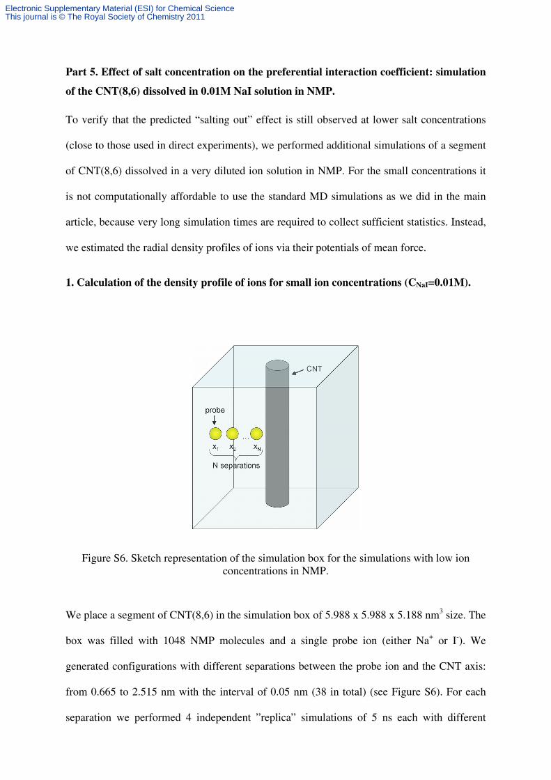
Figure S6. Sketch representation of the simulation box for the simulations with low ion concentrations in NMP.

We place a segment of CNT(8,6) in the simulation box of 5.988 x 5.988 x 5.188 nm3 size. The

box was filled with 1048 NMP molecules and a single probe ion (either Na+ or I-). We

generated configurations with different separations between the probe ion and the CNT axis:

from 0.665 to 2.515 nm with the interval of 0.05 nm (38 in total) (see Figure S6). For each

separation we performed 4 independent ”replica” simulations of 5 ns each with different


initial configurations to improve statistics. The positions of the probe ion and CNT were

fixed. We collected the force acting on the probe ion (each 10th integration step) in the

direction of the vector connecting the ion and the CNT axis (the vector is perpendicular to the

CNT axis). Averaging the force data within the 4 replica simulations we obtained the ”mean

force” on the probe ion as the function of distance from the CNT axis.

Integration of this profile gave us the potential of mean force (PMF, free energy profile) of the

probe ion at the CNT surface (the constant of integration is set such that the average of the

calculated PMF in the interval 2.2 nm < r < 2.5 nm is zero). The corresponding radial density

profiles of the ion at the CNT surface were obtained as:

0

( ) ( )expB

r PMF rk T

ρρ

⎛ ⎞= − ⎜ ⎟

⎝ ⎠,

where PMF(r) is the potential of mean force, kB is the Boltzmann constant, T is the

temperature (300K), �0 is the number density of the corresponding species in the bulk

solutions.

2. MD algorithms details.

We used the same simulation parameters as described in Part 1 of the supporting information,

except for the following. The charge of the single ion in the bulk of NMP molecules in the

simulation box was neutralized by the background compensating charge density uniform

within the simulation box.


3. System preparation and collection of statistics.

In total we had 2 types of probe ions (sodium and iodide) * 38 probe-CNT axis separations *

4 replicas = 304 small simulations.

First, we generated the initial configuration for the system with a Na+ probe ion at 2.515 nm

distance from the CNT axis. The configurations for other separations for the probe ion were

obtained by a short MD simulation where the probe particle was ”pulled” towards the surface

with constant velocity of 0.01 nm/ps. Each configuration was then simulated during 320 ps

simulation time in NVT ensemble at 800K, where the first 120 ps the temperature was

gradually increased from 300K to 800K. Starting from the 120 ps simulation time we stored

the configuration of the systems each 50 ps in a separate file resulting in 4 ''replica``

configurations for each system. The resulting configurations were used as the initial

configurations for the simulations with iodide probe ion. During the 10 ps simulation time the

charge and potential parameters of the Na+ ion were gradually transformed into the potential

parameters of I- ion at 800K. The systems with I- ion were simulated for 90 ps at 800K. For

each replica we performed NVT simulation with gradual decrease of the temperature from

800K to 300K during 100 ps (50 ps) in the case of Na+ (I-) probe ions.

The production run was performed in NVT ensemble at 300K and was 5 ns long for each

small simulation out of 304. The force acting on the probe particle was stored each 10th

integration step.


4. Results.

Figure S7. Mean force acting on the ions in direction connecting the ions and the CNT axis.

a)

b)

Figure S8. Radial density profiles of a) sodium and b) iodide for two studies concentrations of NaI salt.

Table S2 represents the preferential interaction coefficient ( SXΓ ) and the increase of

the CNT surface free energy by addition of the NaI salt into CNT-NMP dispersion ( Sµ∆ ) for


the low salt concentration CNaI=0.01M. The positive value of Sµ∆ indicated that the salt

addition at the small ion concentration leads to the “salting-out” of CNT from the dispersion.

The difference of the KBI integrals (Table S2) is similar for the both salt concentrations; this

proves the CNT free energy increase is linearly proportional to the minus salt concentration

(see equation S10). This explains the experimental observations discussed in the main article

that the increase of the salt concentration increases the degree of the CNT precipitation from

the CNT-NMP dispersions.


Table S2. The difference of the dimensionless ion-CNT and NMP-CNT Kirkwood-Buff integrals ( SX SVG G− ), preferential interaction coefficient ( SXΓ ) and estimated free

energy increase of CNT upon the salt additions ( Sµ∆ ) for three considered systems with

different CNT chiralities and salt concentrations. Note, we calculated the values as averages over the 11 and 4 independent simulations for the 0.15M and 0.01M salt concentrations, correspondingly. We estimated the variances (errors) in the values by the following

expression:

2

1

1

1 1var( )1

simsim

NNii

iisim sim sim

tt t

N N N=

=

⎛ ⎞⎜ ⎟= ⋅ −⎜ ⎟−⎝ ⎠

∑∑ , where t is the value of interest

(following Ref. 26). Note, the differences in the simulation methodologies for the two different salt concentrations.

System: SX SVG G− SXΓ , number of ions

per nm2 Sµ∆ , kBT/nm2

CNT(8,6), C(NaI)=0.15M

-0.55 ± 0.12 -0.12 ± 0.03 0.23 ± 0.06

CNT(6,5), C(NaI)=0.15M

-0.64 ± 0.13 -0.13 ± 0.03 0.26 ± 0.06

CNT(8,6), C(NaI)=0.01M

-0.58 ± 0.10 -0.007 ± 0.003 0.013 ± 0.005


References:

1. Hess, B., Kutzner, C., van der Spoel, D. & Lindahl, E. GROMACS 4: Algorithms for Highly Efficient, Load-Balanced, and Scalable Molecular Simulation. Journal of Chemical Theory and Computation 4, 435-447 (2008).

2. Frey, J.T. & Doren, D.J. TubeGen Online v3.4 (web-interface), University of Delaware, Newark DE, 2011. at <http://turin.nss.udel.edu/research/tubegenonline.html>

3. Jorgensen, W.L. & Severance, D.L. Aromatic-aromatic interactions: free energy profiles for the benzene dimer in water, chloroform, and liquid benzene. Journal of the American Chemical Society 112, 4768-4774 (1990).

4. Schrödinger Maestro. at <http://www.schrodinger.com/> 5. Gromacs 4, Manual. at <http://www.gromacs.org/> 6. Shih, C.-J., Lin, S., Strano, M.S. & Blankschtein, D. Understanding the Stabilization of

Liquid-Phase-Exfoliated Graphene in Polar Solvents: Molecular Dynamics Simulations and Kinetic Theory of Colloid Aggregation. Journal of the American Chemical Society 132, 14638-14648 (2010).

7. Jensen, K.P. & Jorgensen, W.L. Halide, Ammonium, and Alkali Metal Ion Parameters for Modeling Aqueous Solutions. Journal of Chemical Theory and Computation 2, 1499-1509 (2006).

8. Essmann, U. et al. A Smooth Particle Mesh Ewald Method. Journal of Chemical Physics 103, 8577–8593 (1995).

9. Hess, B., Bekker, H., Berendsen, H. & Fraaije, J. LINCS: A linear constraint solver for molecular simulations. Journal of Computational Chemistry 18, 1463-1472 (1997).

10. Bussi, G., Donadio, D. & Parrinello, M. Canonical sampling through velocity rescaling. The Journal of Chemical Physics 126, 014101 (2007).

11. Berendsen, H., Postma, J., van Gunsteren, W., DiNola, A. & Haak, J. Molecular dynamics with coupling to an external bath. The Journal of Chemical Physics 81, 3684-3690 (1984).

12. Martínez, L., Andrade, R., Birgin, E.G. & Martínez, J.M. PACKMOL: a package for building initial configurations for molecular dynamics simulations. J Comput Chem 30, 2157-2164 (2009).

13. Frolov, A.I., Rozhin, A.G. & Fedorov, M.V. Ion Interactions with the Carbon Nanotube Surface in Aqueous Solutions: Understanding the Molecular Mechanisms. ChemPhysChem 11, 2612-2616 (2010).

14. Parsegian, V.A., Rand, R.P. & Rau, D.C. Osmotic stress, crowding, preferential hydration, and binding: A comparison of perspectives. Proceedings of the National Academy of Sciences of the United States of America 97, 3987–3992 (2000).

15. Pal, S. & Müller-Plathe, F. Molecular Dynamics Simulation of Aqueous NaF and NaI Solutions near a Hydrophobic Surface. The Journal of Physical Chemistry B 109, 6405-6415 (2005).

16. Kirkwood, J.G. & Buff, F.P. The Statistical Mechanical Theory Of Solutions .1. Journal of Chemical Physics 19, 774–777 (1951).

17. Shimizu, S., McLaren, W.M. & Matubayasi, N. The Hofmeister series and protein-salt interactions. J. Chem. Phys. 124, 234905 (2006).

18. Schurr, J.M., Rangel, D.P. & Aragon, S.R. A Contribution to the Theory of Preferential Interaction Coefficients. Biophysical Journal 89, 2258-2276 (2005).

19. Shulgin, I. & Ruckenstein, E. A protein molecule in a mixed solvent: the preferential binding parameter via the Kirkwood-Buff theory. Biophysical Journal 90, 704-707 (2006).


20. Matubayasi, N., Shinoda, W. & Nakahara, M. Free-energy analysis of the molecular binding into lipid membrane with the method of energy representation. J. Chem. Phys. 128, 195107 (2008).

21. Ben-Naim, A. Molecular Theory of Solutions. (Oxford University Press, USA: 2006). 22. Chitra, R. & Smith, P.E. Preferential Interactions of Cosolvents with Hydrophobic

Solutes. The Journal of Physical Chemistry B 105, 11513-11522 (2001). 23. Kusalik, P.G. & Patey, G.N. The thermodynamic properties of electrolyte solutions: Some

formal results. The Journal of Chemical Physics 86, 5110 (1987). 24. Tan, P.H. et al. Photoluminescence Spectroscopy of Carbon Nanotube Bundles: Evidence

for Exciton Energy Transfer. Phys. Rev. Lett. 99, 137402 (2007). 25. Hasan, T. et al. Nanotube-Polymer Composites for Ultrafast Photonics. Advanced

Materials 21, 3874–3899 (2009). 26. Frenkel, D. & Smit, B. Understanding Molecular Simulation: From Algorithms to

Applications. (Academic Press Inc: 1996).


molecular mechanisms of salt effects on carbon …6,5) of 4.067 nm long solvated in pure nmp...

Documents