MOLFLOW SEMINARMonte Carlo simulation of ultra high vacuum systems

2014.11.26, KEK - Marton Ady

VACUUM CALCULATIONS: ANALYTICAL METHOD

S S SL

A

Q=C*(p1-p2)P=Q/S

VACUUM CALCULATIONS: ANALYTICAL METHOD

S S SL

A

Q=C*(p1-p2)P=Q/S

Q(x)=-C*dP/dx

VACUUM CALCULATIONS: ANALYTICAL METHOD

S S SL

A

DIFFICULTY: CONDUCTANCE

DIFFICULTY: CONDUCTANCE

Geometry: polygonsMC SIMULATIONS

Geometry: polygons Gas input:

pV=NkT

1 Pa*m3/s = 2.4*1020 molecules/s

Virtual / Physical particle ratio

MC SIMULATIONS

Ray-plane intersection:

-  Use Cramer�s rule to find I coordinates.

vuw ∧=-  is pre-calculated once for each facet.

]1,0[.

).(∈

∧=

rw

rvOI fru

]1,0[.

).(∈

∧=

rw

rOuI frv

0.

.>−=

rw

OwI frr

-  Faster to solve Iu and Iv first (best elimination method than solving distance Ir first).

AABB Tree optimisation:

-  Use of �Axis Aligned Bounding Box� tree structure to speed collision detection -  Box/ray intersection performed using the �slabs method�

-  Minimum of 8 facets per box and maximum tree depth of 5 (using �best axis� method for AABB tree balancing)

-  Result: more than 5 times faster for complex geometries

Ray tracing

Reflection

S [m3/s] = sticking [0..1] * 1/4 * A [m2] * vavg [m/s]

Pumping / absorption

Reflection

Collecting statistics

MolFlow SynRad

Molflow (1990)

Roberto Kersevan

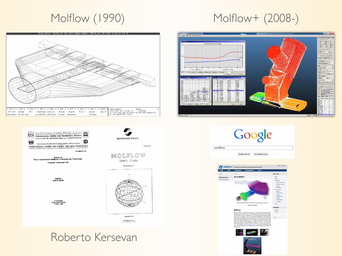
Molflow (1990)

Roberto Kersevan

Molflow+ (2008-)

molflow

Step 1: creating geometry

CAD Molflow+

STL format

WORKING WITH MOLFLOW

Step 2: adding physicsWORKING WITH MOLFLOW

Step 3: simulation and resultsWORKING WITH MOLFLOW

Step 3: simulation and resultsWORKING WITH MOLFLOW

Step 3: simulation and resultsWORKING WITH MOLFLOW

Step 3: simulation and resultsWORKING WITH MOLFLOW

Step 3: simulation and resultsWORKING WITH MOLFLOW

Step 3: simulation and resultsWORKING WITH MOLFLOW

Step 3: simulation and resultsWORKING WITH MOLFLOW

Step 3: simulation and resultsWORKING WITH MOLFLOW