monetary analysis: tools and applications - european central bank
TRANSCRIPT

First ECB Central Banking Conference
November 2000, Frankfurt, Germany
Monetary Analysis:Tools and Applications
Editors:Hans-Joachim Klöckers
Caroline WillekeLex HoogduinJulian Morgan
Bernhard Winkler

Published by:© European Central Bank, August 2001Address Kaiserstrasse 29
60311 Frankfurt am MainGermany
Postal address Postfach 16 03 1960066 Frankfurt am MainGermany
Telephone +49 69 1344 0Internet http://www.ecb.intFax +49 69 1344 6000Telex 411 144 ecb d
Copies of the individual articles can also be downloaded from the ECB’s website.
The views expressed in this publication are those of the authors and not necessarily those of the ECB.No responsibility for them should be attributed to the ECB or to any of the other institutions with whichthe authors are affiliated.
All rights reserved by the authors.
Editors:Hans-Joachim KlöckersCaroline Willeke
Typeset and printed by:Druckhaus Thomas Müntzer GmbH
ISBN 92-9181-148-3
Foreword “The importance of monetary analysis”O. Issing (European Central Bank) . . . . . . . . . . . . . . . . . . . . . . . . . . . . . . . . . . . . . . . . . . 5
PrefaceH.-J. Klockers (European Central Bank) . . . . . . . . . . . . . . . . . . . . . . . . . . . . . . . . . . . . . 9
Summary “Monetary analysis: tools and applications”H. Pill (European Central Bank) . . . . . . . . . . . . . . . . . . . . . . . . . . . . . . . . . . . . . . . . . . . . 11
“Uncertainty and multiple perspectives”J. Selody (Bank of Canada) . . . . . . . . . . . . . . . . . . . . . . . . . . . . . . . . . . . . . . . . . . . . . . . . 31
“The role of M3 in the policy analysis of the Swiss National Bank”T. Jordan, M. Peytrignet and Georg Rich (Swiss National Bank) . . . . . . . . . . . . . . . . 47
“Money and credit in an inflation-targeting regime:The Bank of England’s Quarterly Monetary Assessment”A. Hauser (Bank of England) . . . . . . . . . . . . . . . . . . . . . . . . . . . . . . . . . . . . . . . . . . . . . . 63
“Money and inflation: the role of information regarding the determinantsof M2 behaviour”A. Orphanides and R. D. Porter (Board of Governorsof the Federal Reserve System) . . . . . . . . . . . . . . . . . . . . . . . . . . . . . . . . . . . . . . . . . . . . . 77
“The impact of financial anxieties on money demand in Japan”T. Kimura (Bank of Japan) . . . . . . . . . . . . . . . . . . . . . . . . . . . . . . . . . . . . . . . . . . . . . . . . . 97
“Framework and tools of monetary analysis”K. Masuch, H. Pill and C. Willeke (European Central Bank) . . . . . . . . . . . . . . . . . . . 117
“Monetary analysis in the Bank of Italy prior to EMU:The role of real and monetary variables in the models of the Italian economy”F. Altissimo, E. Gaiotti and A. Locarno (Banca d’Italia) . . . . . . . . . . . . . . . . . . . . . . . 145
“The role of the analysis of the consolidated balance sheet of the banking sectorin the context of the Bundesbank’s monetary targeting strategy prior to Stage Three”J. Reischle (Deutsche Bundesbank) . . . . . . . . . . . . . . . . . . . . . . . . . . . . . . . . . . . . . . . . . 165
Table of Contents

“The integration of analysis of extended monetary and credit aggregatesin the experience of the Banque de France”F. Drumetz and I. Odonnat (Banque de France) . . . . . . . . . . . . . . . . . . . . . . . . . . . . . . 187
“Flow of funds analysis in the experience of the Banco de Espana”J. Penalosa and T. Sastre (Banco de Espana) . . . . . . . . . . . . . . . . . . . . . . . . . . . . . . . . . 209
List of Participants . . . . . . . . . . . . . . . . . . . . . . . . . . . . . . . . . . . . . . . . . . . . . . . . . . . . . . . . 223
4 Table of Contents

These days, few economists would disagree with the statement that inflation is a mone-tary phenomenon in the long run. Indeed, this statement is one of the central tenets ofeconomic theory. The long-run relationship between money and prices has been con-firmed by an impressive number of empirical studies, both across countries and acrosstime. Moreover, the ability to implement monetary policy ultimately hinges on a centralbank’s monopoly control over the creation of base money. Given the fundamentalmoney-prices relationship and their monopoly power over the legal tender, the mone-tary authorities have a natural interest in monetary developments. At a more practicallevel, monetary data are collected in a timely manner and are more accurate than manyother economic indicators. All these factors explain why money plays a prominent rolein monetary policy-making and thus why the monetary analysis undertaken at centralbanks is both necessary and important.The monetary policy strategy of the ECB recognises the monetary nature of inflation
by assigning a prominent role to money in the formulation of monetary policy decisionsaimed at the maintenance of price stability. This prominence is signalled by the an-nouncement of a quantitative reference value for the growth rate of the broad mone-tary aggregate M3. In December 1998 the Governing Council of the ECB has set thisreference value at 4 +% and this value was subsequently confirmed in 1999 and 2000.A detailed analysis of monetary developments with the aim of extracting the informa-tion relevant for monetary policy decisions represents the first “pillar” of the ECB’smonetary policy strategy. Among other things, this analysis includes an investigation ofthe deviation of M3 growth from the reference value.Monetary analysis begins with the very definition of a key monetary aggregate.
While it is easy to speak about the “M” which appears in economics textbooks, it ismuch harder in practice to give a meaningful definition of a monetary aggregate. Thereis now a consensus that broad aggregates, such as euro area M3, tend to perform betteras monetary policy indicators than do narrower measures of money, since they interna-lise the portfolio shifts pervasive in a world of financial innovation and rapid change. Inparticular, econometric evidence suggests that euro area M3 both has a stable relation-ship with the price level in the long run and possesses leading indicator properties forinflation over the medium term. As such, this aggregate has the properties required todefine the reference value and thus to signal the prominent role of money in the ECB’smonetary policy.To a large extent, monetary analysis represents the analytical work necessary to de-
termine from the available monetary data the underlying relationship between money
Foreword
The importance of monetary analysis
Otmar Issing
Member of the Executive Board of the European Central Bank

and the price level. Monetary developments may be subject to a host of special influ-ences and distortions which render the relationship between money and prices complexin the short run. Extracting the stable long-run relationship – say between euro areaM3 and the euro area price level – from shorter-term developments in M3 is, in es-sence, the filtering of signals from noise. This analysis is demanding, since it requiresboth a strong command of economic theory and a detailed knowledge of the institu-tional environment. In particular, monetary analysis should always encompass a closemonitoring of financial innovation as this may affect the fundamental relationship be-tween money and prices.To implement this more detailed assessment, monetary analysis undertaken at the
ECB is not limited solely to the analysis of M3. The main components and counterpartsof M3 in the balance sheet of the Monetary Financial Institutions sector are also closelymonitored. In particular, the developments of credit to the private sector and of themost liquid components of M3, included in the narrow monetary aggregate M1, arefollowed with particular attention. This broader analysis is necessary to put develop-ments into perspective, to obtain a better understanding of M3 developments and,more generally, to develop a broader insight into monetary conditions and their impli-cations for monetary policy decisions aimed at maintaining price stability.Monetary analysis can provide many kinds of information. Used as an indicator,
monetary developments may signal risks to future price stability. Furthermore, mone-tary analysis may also be useful to monitor (and possibly offset) macroeconomic riskswhich are not directly related to price stability stricto sensu, but which may neverthelesshave important consequences. For instance, historical experience has shown that boomsand busts in capital markets, often associated with phenomena of excessive enthusiasmor excessive pessimism about the future, have typically been accompanied by largeswings in monetary and credit aggregates.A broader analysis of the flow of funds may also provide important inputs. In fact,
by providing an insight into the composition of the balance sheet of the main actors inthe economy (households, firms and intermediaries), a flow of funds analysis can helpto assess the likely impact of interest rate changes on spending decisions, allowing adeeper understanding of the monetary policy transmission and therefore a proper cali-bration of monetary policy instruments. So far, the unavailability of the necessary datahas prevented the ECB from carrying out a fully-fledged flow of funds analysis for theeuro area as a whole, but the situation should improve substantially in this regard innot too distant a future.At the ECB, detailed monetary analysis and the announcement of a reference value
for M3 growth are closely interwoven, since the reference value constitutes per se acommitment to analyse monetary data carefully. It shows that monetary growth – theultimate source of inflation in the long run – is taken seriously in the policy-makingprocess. Given that the link between money and prices has a long-run nature, it alsosignals that monetary policy has an appropriate medium-term orientation. This, in turn,contributes to shaping agents’ expectations in a manner which enhances the credibilityof the central bank.The experience of the first two years of Stage Three of Economic and Monetary
Union (EMU) has shown that monetary developments in the euro area – and in parti-cular the deviation of M3 growth from the reference value of 4 +% – have providedconsistent and reliable guidance for monetary policy. Interest rate decisions by the ECB
6 Otmar Issing
Governing Council have been supported by remarkably consistent information fromthe first pillar of the ECB’s monetary policy strategy. At the same time, some cautionneeds to be exercised since M3 developments have presumably been influenced onoccasion by special factors and distortions. For example, the exceptionally strong rise inM3 growth in January 1999 may have been due, in part, to the special environment atthe start of Stage Three of EMU (e.g. the change in the reserve requirement regimeassociated with the introduction of the Eurosystem’s operational framework).All these considerations demonstrate why monetary analysis is important and, at the
same time, show what difficult and far-reaching questions it is expected to answer. In-deed, many issues remain unsettled in economics literature and definitive answers arenot easy to find. Nevertheless, there can be no doubt that monetary analysis should beassigned an important role in shaping the monetary policy debate.
The importance of monetary analysis 7


On 20 and 21 November 2000, the ECB’s Directorate Monetary Policy organised a semi-nar for central banks on “Monetary analysis: tools and applications”. The aim of the semi-nar was to obtain an overview of the various approaches used to assess monetary develop-ments in major central banks. The seminar involved presentations and discussions by staffmembers from the ECB, EU national central banks and other G10 central banks.
As it emerged that the papers submitted to the seminar were of more general inter-est, it was deemed useful to make them available to the public. This volume presentsthe ten papers prepared for the seminar, together with a summary highlighting themain themes.
I drew a number of personal conclusions from the seminar. The most important wasto see that monetary analysis continues to be “en vogue” among central bankers. Asthe papers show, the world’s main central banks conduct some form of monetary analy-sis, with an increasing degree of depth and sophistication.
The seminar showed the variety of approaches adopted for the analysis of monetarydevelopments. The tools used range from relatively sophisticated econometric methods tovery detailed analyses of institutional factors, monetary counterparts, broader aggregates(on both the credit and the investment side), and flows of funds, etc. Particular impor-tance was also given in some countries to the use of sectoral monetary data. All theseapproaches appear interesting and promising. However, the Eurosystem still has someway to go to increase the availability of harmonised monetary and financial statistics forthe euro area in order to be in a position to replicate all the analyses conducted by othercentral banks.
As reflected in the contributions to the seminar, differences exist with regard to theapproach adopted by central banks to combine monetary analysis with analyses of othereconomic and financial data in order to prepare monetary policy decisions. At one ex-treme, at some central banks this analysis is combined at the staff level, with the role of themonetary analysis in the overall assessment remaining to some extent hidden from thedecision-maker. At the other extreme, the two forms of analysis are combined only at thelevel of the decision-maker, or even beyond, in the public discussion of monetary policy.
The seminar showed that these differences relate very much to past experiences inindividual countries with the reliability of monetary indicators. However, some of thepapers presented at the seminar demonstrated that even in countries where money hason certain occasions appeared to be rather unpredictable (e.g. in the United States andJapan), a deeper analysis of underlying factors could help in finding stable relationships,and this not only ex post.
Preface
Hans-Joachim Klockers
European Central Bank

Finally, a crucial issue raised at the seminar was how monetary analysis should bepresented to the public. There is a trade-off here between the complexity of many ofthe econometric models and the need to communicate in a simple and comprehensiblemanner. The ECB has chosen to signal the prominent role for money by announcing areference value for M3. While other approaches are possible, the ECB’s choice is wellfounded given the empirical evidence with regard to the close relationship between M3and price developments in the euro area.
In sum, I am convinced that the seminar helped to stimulate thinking within manycentral banks on how to make monetary analysis most useful. In any case, for the ECBand for the Eurosystem as a whole the seminar gave rise to a lot of ideas for furtherdeveloping its work, both internally and with regard to its external presentation.
At this point, I should once again like to thank all those who participated in theseminar (a list of whom is included at the end of the volume) for their contributions,whether in the form of the papers presented in this volume or with regard to theiractive involvement in the discussions. At the ECB, I should like to express specialthanks to Caroline Willeke and Claire Burns, who, together with Claus Brand, DieterGerdesmeier, Jose Luis Escriva, Klaus Masuch, Huw Pill and Livio Stracca, took overmost of the burden involved in the practical organisation of the seminar.
November 2000
10 Hans-Joachim Klockers

1. Introduction
“We did not abandon M1. M1 abandoned us.”Gerald Bouey, former Governor of the Bank of Canada, March 1983.1
“Inflation is ultimately a monetary phenomenon. The Governing Council therefore recog-nised that giving money a prominent role in the Eurosystem’s strategy was important.”
ECB Monthly Bulletin, January 1999, p. 47.
These two quotations illustrate the breadth of central bank opinion on the role ofmoney in monetary policy-making. On the basis of a central bank workshop held inFrankfurt during November 2000, this paper goes behind such rhetoric to consider therole monetary analysis plays in monetary policy.On the one hand, Mr. Bouey’s above oft-quoted remark is indicative of the frustra-
tion felt by many central banks pursuing monetary targets in the early 1980s. The con-siderable challenges faced by intermediate monetary targeting strategies during this per-iod have been well documented in the academic literature, particularly for the Anglo-Saxon countries (e.g. Goodhart, 1989). In an environment of financial innovation andstructural change, changes in financial structure created instabilities in money demandwhich rendered developments in the monetary aggregates difficult for policy makers tointerpret, let alone explain coherently and consistently to the public. These practicaldifficulties led several Anglo-Saxon central banks to abandon formal monetary targetsin the mid and late 1980s. Furthermore, in many countries – regardless of whether for-mal targets had been announced – the importance attached to monetary indicators as aguide to monetary policy decisions progressively diminished. The British experience inthis regard, culminating in the abolition of the remaining “monitoring ranges” for thegrowth of monetary aggregates in 1997, is instructive, but by no means unique. Forexample, the US Federal Reserve, while still announcing ranges for monetary and credit
Summary
Monetary analysis: tools and applications
Huw Pill*
European Central Bank
* This paper summarises the proceedings of the ECB central bank workshop “Monetary analysis:tools and applications” held at the ECB in Frankfurt on 20–21 November 2000. It has benefitedfrom the comments and suggestions of Hans-Joachim Klockers, Klaus Masuch, Jose-Luis Escriva,Caroline Willeke, Livio Stracca, Dieter Gerdesmeier and other colleagues in the ECB’s Directo-rate Monetary Policy. The views expressed in the paper are those of the authors and do not neces-sarily reflect the views of the ECB or the Eurosystem.
1 Quoted from the Minutes of Proceedings and Evidence of the Canadian House of CommonsStanding Committee on Finance, Trade and Economic Affairs, No. 134, 28 March 1983, p. 12.
growth as required by legislation, also assigned monetary developments a lesser role inpolicy decisions, especially from the early 1990s onwards, and eventually abolished theannouncement of the ranges in July 2000.2
On the other hand, the European Central Bank (ECB) statement quoted above is areflection of a different experience. In continental Europe monetary and credit aggre-gates continued to play an important role in the conduct of monetary policy throughoutthe 1980s and 1990s. In particular, the Deutsche Bundesbank – maintaining the inter-mediate monetary targeting strategy which it had pursued with success since the mid-1970s – continued to announce a target for the growth rate of its broad monetaryaggregate M3 until the end of 1998 (when the responsibility for monetary policy passedto the ECB). Other continental European central banks (including the Banque deFrance, the Banca d’Italia and the Banco de Espana) also announced monetary targetsor reference ranges which complemented and supported other aspects of their mone-tary policy strategies, such as exchange rate targets and/or direct inflation targets.The continued prominence of money and monetary aggregates in the monetary pol-
icy strategies of continental European central banks was a reflection of the empiricalproperties demonstrated by the monetary aggregates – in particular, the continued sta-bility of money demand and the leading indicator properties of monetary developmentsfor future inflation. These empirical characteristics were markedly different from thoseobserved in many Anglo-Saxon countries. In the latter, it became almost “conventionalwisdom” (at least in the journalistic and academic discussion) that monetary develop-ments were largely “noise”, which was naturally of little relevance for monetary policydecisions aimed at price stability. In this light, several countries – notably the UnitedKingdom and Canada – adopted direct inflation targeting strategies in the early 1990s,since monetary aggregates and other indicators no longer appeared to constitute plausi-ble or meaningful intermediate targets.It was against this background that, first, the Committee of Governors of the Central
Banks of the Member States of the European Community and, later, the EuropeanMonetary Institute (EMI) undertook the preparatory work required for the introduc-tion of the euro and the creation of the single European monetary policy. Naturally,one aspect of this preparatory work was an analysis of the pros and cons of variousmonetary policy strategies which could form the basis of the ECB’s approach to mone-tary policy. Attention focused on the relative merits of direct inflation targeting andintermediate monetary targeting, which were widely viewed as the two plausible candi-date strategies for the ECB.However, in comparing the relative merits of inflation and monetary targeting, the
EMI (1997) recognised that the sharp distinction drawn in the academic literature wasmisleading. This conclusion followed from the observation that central banks targetinginflation, at least in their internal analyses, devote considerable resources to monitoring
12 Huw Pill
2 Quoting from the U.S. Federal Reserve Board of Governors July 2000 Report to Congress:“At its June meeting, the FOMC did not establish ranges for growth of money and debt in 2000and 2001. The legal requirement to establish and to announce such ranges had expired, and owingto uncertainties about the behavior of the velocities of debt and money, these ranges for manyyears have not provided useful benchmarks for the conduct of monetary policy. Nevertheless, theFOMC believes that the behavior of money and credit will continue to have value for gaugingeconomic and financial conditions, and this report discusses recent developments in money andcredit in some detail.”

and analysing monetary developments. At the same time (as illustrated by Reischle(Deutsche Bundesbank) in this volume for the case of the Bundesbank), central bankspursuing intermediate monetary targets also evaluated a very broad range of economicand financial indicators beyond the key monetary aggregate in coming to their mone-tary policy decisions.Against this background, in October 1998 – after a comprehensive evaluation of
central bank experience and an assessment of the particular circumstances of the euroarea – the Governing Council of the ECB decided to adopt neither monetary targetingnor inflation targeting, but rather its own stability-oriented monetary policy strategy(ECB, 1999a). The primary and overriding objective of the single monetary policy isthe maintenance of price stability in accordance with a definition published by theECB. Within the two-pillar framework created by the ECB’s strategy, risks to pricestability are assessed, on the one hand, on the basis of an analysis of monetary develop-ments (the first pillar of the strategy) and, on the other hand, by an assessment ofother economic and financial indicators (the second pillar). The prominent role ofmoney in the ECB’s strategy is signaled by the announcement of a quantitative refer-ence value for the growth rate of the broad monetary aggregate M3.In their public presentation of monetary policy, most central banks currently assign
monetary aggregates a less important role in the explanation of monetary policy deci-sions than does the ECB. In particular, they neither officially accord money a promi-nent role nor publicly announce a reference value for monetary growth. Nevertheless, abroad spectrum of approaches exists.On the one hand, the Swiss National Bank (SNB) gives the broad monetary aggre-
gate M3 “a major role as a monetary policy indicator”3, and is therefore perhaps clo-sest in approach to the ECB. On the other hand, many other central banks do notaccord a prominent role to money, focusing at least in their public statements almostexclusively on an analysis of the interaction of demand and supply and cost pressuresin the real economy and/or a published inflation forecast based on such analysis.Against this background, the ECB’s Directorate Monetary Policy in the Directorate
General Economics organised a central bank workshop in November 2000 to discussthe role of monetary analysis in the monetary policy making processes of centralbanks. Staff members from each of the EU central banks, the U.S. Board of Gover-nors of the Federal Reserve System, the Bank of Canada, the Bank of Japan andthe SNB were invited. The purpose of the workshop was twofold. First, it encour-aged comparison of the tools and techniques of monetary analysis employed at var-ious central banks, permitting an exchange of views and ideas of mutual benefit.Second, the workshop was intended to provide a platform for discussing the role ofmonetary analysis in monetary policy strategies in general, and in the ECB’s strategyin particular.One purpose of this paper – and the accompanying papers contained in this volume
– is to extend this clarification of the role and nature of monetary analysis to a broaderaudience, encompassing those outside the central banking community. It therefore sum-marises the proceedings of the workshop and comments on them from the perspectiveof an ECB staff member.
Monetary analysis: tools and applications 13
3 Statement of the monetary policy strategy of the SNB, available at http://www.snb.ch/e/geldpo-litik/geldpol.html.
The remainder of the paper is organised as follows. Section 2 notes that there aremany similarities among central banks in their internal work. In particular, a broadconsensus exists that monetary developments reveal relevant information for monetarypolicy decisions aimed at price stability (or inflation) objectives. In addition, it suggeststhat extracting the relevant information requires the adoption of relatively sophisticatedtechniques. Section 3 focuses on differences between central banks, relating in particu-lar to the way monetary analysis is combined with analyses of other economic andfinancial indicators, and to how monetary analysis and its role in the policy process ispresented to the public. Section 4 briefly concludes.
2. Similarities across central banks: the importance and complexityof monetary analysis
2.1. All central banks monitor monetary developments closely
All the central banks participating in the workshop – regardless of the monetary policystrategy that they formally pursue – recognise that monetary developments contain in-formation which is potentially important for taking monetary policy decisions aimed atthe maintenance of price stability. All central banks therefore closely analyse monetarydevelopments on a regular basis. In particular, contrary to characterisations typical ofthe academic literature, central banks targeting inflation (e.g. the Bank of England, theBank of Canada) analyse monetary developments thoroughly.
2.2. . . . but the approach to monetary analysis can differ . . .
The type of information contained in monetary developments can be seen as lyingalong a spectrum, ranging from, on the one hand, a structural explanation of the infla-tion process where money plays an active and dominant part, to, on the other hand, atreatment of money as, at most, a summary indicator with little or no causal role in thedetermination of price developments.As recognised by Friedman (1984), monetary aggregates can play an important role
as indicators even if they play no structural or causal role in the inflation process or thetransmission mechanism for monetary policy. Even if inflation is regarded solely as theresult of excess demand or cost pressures, monetary developments can still provideinformation for monetary policymaking if they allow central banks to identify better thenature of shocks hitting the economy, and/or to predict trends in future price develop-ments and thus identify emerging risks to price stability.One explanation of the leading indicator properties of money for future inflation is
that monetary indicators may be related to observable macroeconomic variables thatplay an important role in the transmission mechanism, such as real economic activity orinterest rates. For example, money demand studies suggest that monetary growth isrelated (positively) to real GDP growth and (negatively) to interest rates. In this con-text, GDP growth above sustainable rates will typically increase both monetary growthand inflationary pressures. Similarly, inappropriately low levels of interest rates mayboth spur monetary growth and lead to risks to price stability. Viewed in this light,monetary growth summarises information about developments in the determinants ofmoney demand, which also influence future price developments. Such a summary vari-able can therefore be a useful indicator for monetary policy.
14 Huw Pill
While such a summary statistic role is useful, monetary developments may also pos-sess additional information about future price developments beyond that which is con-tained in other macroeconomic indicators. In this volume, this approach is adopted byOrphanides and Porter (Federal Reserve Board), Jordan, Peytrignet and Rich (SwissNational Bank) and Altissimo, Gaiotti and Locarno (Banca d’Italia). These papers high-light the role of monetary aggregates as informational variables, which can provideadditional or complementary information to that derived from conventional macro-economic models.One approach to investigating this role for money is pursued by Altissimo et al. for
the case of Italy. Following a suggestion by Friedman (1984), they investigate whetherthe residuals from money and credit demand equations embedded in the Banca d’Ita-lia’s large macroeconometric model of the Italian economy are correlated with forecasterrors for key macroeconomic variables, such as inflation and GDP growth. Such corre-lations are found. Therefore, although the Banca d’Italia model does not accord mone-tary variables an “active” causal role in the transmission mechanism, this exercisenevertheless suggests that there is information in monetary developments beyond thatin the determinants of money which helps to forecast macroeconomic variables of inter-est to central banks.The results reported by Altissimo et al. can be interpreted as suggesting that mone-
tary and credit developments reveal information about factors which are important forthe transmission mechanism – such as interest rate spreads or non-price rationing ofcredit – yet are neither easily measured (and thus for which statistics are typically notavailable) nor captured by conventional macroeconometric models. In such circum-stances, residuals to money demand equations provide relevant “news” to policy ma-kers.Monetary and credit variables may also play an active role in the inflation process
and/or the transmission mechanism for monetary policy. In this context, central banksare likely to find it important to monitor monetary variables in order to obtain abetter insight into the structural and behavioural relationships underlying these pro-cesses. For example, if bank credit is sometimes rationed using non-price mechanisms(e.g. as investigated in the credit rationing literature following from Stiglitz and Weiss(1981)), monitoring credit aggregates should help to develop a better understandingof the economic situation and the likely impact of monetary policy actions, both ofwhich are, of course, crucial to well-designed policy decisions aimed at the mainte-nance of price stability.Some approaches to extracting the information in money represent an amalgam of
the “summary statistic” and “additional information” views. The indicator properties ofmonetary growth for price developments in the euro area are investigated by NicolettiAltimari (2001) in a simulated out-of-sample forecasting exercise. His results are re-ported in this volume by Masuch, Pill and Willeke (ECB). They suggest that euro areaM3 growth is one of the best predictors of cumulative inflation over the coming threeyears, out-performing cost and demand indicators (such as unit labour costs and esti-mates of the output gap), as well as a variety of other monetary indicators. The studytherefore supports the view that price developments over the medium term can be pre-dicted on the basis of monetary indicators. Evaluating the indicator properties of head-line monetary growth, e.g. in the manner of Nicoletti Altimari (2001), may capture boththe summary statistic and additional information contained in M3 growth.
Monetary analysis: tools and applications 15

2.3. . . . and a variety of relatively complex approaches are employed . . .
In practice, central banks adopt a pragmatic approach to monetary analysis, encompass-ing both the structural and informational variable views. The range of approaches em-ployed within a single central bank is therefore typically rather large. On the basis ofexperience at the Bank of England and the ECB respectively, the papers presented byHauser (Bank of England) and Masuch, et al (ECB) describe a broad variety of timeseries models which use money to help predict the path of future inflation, GDPgrowth and other important macroeconomic variables. While this eclectic approach fallsshort of providing a single framework for monetary analysis, it helps to ensure that asmuch relevant information as possible is extracted from monetary developments.
2.4. . . . which embody a judicious mixture of econometric techniques . . .
The range of analytical tools and techniques available for monetary analysis is poten-tially extremely broad. Several papers presented at the workshop illustrated specificmodel applications, while others gave a wider overview of the type of models used inthe analyses underlying monetary policy decisions.A natural starting point for econometric modeling of monetary developments is the esti-
mation of money demand equations. An enormous academic literature now exists (Gold-feld and Sichel (1990) and Laidler (1993) provide general surveys; Browne, et al. (1997)review the literature relating to EU countries). Central banks have made many importantcontributions to this literature. Recent papers have almost ubiquitously relied on errorcorrection specifications and used time series modeling techniques based on cointegration.Kimura’s (Bank of Japan) paper in this volume provides an elegant example of this
approach in an investigation of the stability of money demand in Japan during the1990s. Consistent with the results described by other participants in the workshop, hedemonstrates that an “intelligent interpretation” of monetary developments in Japan –which in this case accords an important role to the impact of financial volatility on theprecautionary demand for money – can account for the evolution of M2 + CDs (thekey aggregate monitored by the Bank of Japan) over the last decade. This result over-turns the finding (based on more conventional specifications) that money demand inJapan has been unstable in recent years.As noted above, the Hauser and Masuch, et al. papers provide a broad overview of
the econometric techniques developed and used for monetary analysis by staff at theBank of England and the ECB respectively. The techniques employed are revealed tobe very similar. Both the Bank of England and the ECB use a variety of money-basedtime series indicator models for inflation and other macroeconomic variables. Consis-tent with the mainstream academic literature, the two main econometric frameworksdiscussed are vector autoregressions (VARs) and vector error corrections models(VECMs) (Dhar, et al., 2000; Brand and Cassola, 2000). Both these approaches areused to investigate the indicator properties of monetary and credit aggregates formacroeconomic developments, typically in conjunction with developments in other indi-cators. The main difference between the two types of model is that VECMs imposelong-run relationships between the money stock, prices and other key economic vari-ables (e.g. in the form of a money demand equation), whereas VARs focus on shorter-term dynamic interactions.
16 Huw Pill
While the techniques employed are similar, some nuances emerge. On the one hand,the Bank of England places greater emphasis on analysis and modeling of sectoral ag-gregates. (For the time being, the scope for such analysis at the ECB for the euro arearemains restricted by the lack of long-run time series for sectoral money and credit atthe area-wide level.) On the other hand, the ECB has placed greater emphasis on eval-uating the leading indicator properties of a wide variety of monetary and credit indica-tors in simulated out-of-sample exercises, as proposed by Stock and Watson (1999)(Nicoletti Altimari, 2001).One prominent variant of the VECM approach is the so-called P-star model of infla-
tion (Hallman, et al., 1991). As illustrated in several papers presented at the workshop,such models use the deviation of the money stock from a level deemed consistent withequilibrium as a leading indicator of future inflation. The P-star model is used at sev-eral central banks, including the Federal Reserve System, the ECB, the SNB and theBank of Japan.For example, Kimura uses his money demand results to derive a measure of the
equilibrium money stock and thus a P-star indicator for Japanese inflation. On the basisof this indicator, he demonstrates that monetary developments, appropriately correctedfor the impact of financial volatility, are a leading indicator of inflation in Japan. Simi-larly, in their study of Swiss data, Jordan, et al. show that a P-star model can forecastprice developments at a one to two-year horizon, a result confirmed for the euro areaby Gerlach and Svensson (2000), Trecroci and Vega (2000) and Nicoletti Altimari(2001).In illustrating the performance of the P-star model in the United States, Orphanides
and Porter make two important points.First, they demonstrate that, in order to obtain good forecasts of inflation, the equili-
brium level of M2 income velocity has to be modeled in a time-varying manner, ratherthan be treated as a constant as in the original P-star model (Hallman, et al., 1991).This is consistent with the results obtained by other central banks, which use moneydemand equations to predict developments in the equilibrium velocity concept under-lying the P-star approach.Orphanides and Porter show that a shift in M2 income velocity in the early 1990s –
associated with innovations in the financial and banking sector – severely disrupts thesimple P-star model’s forecasting performance. This basic story is a familiar one: finan-cial innovation can lead to changes in equilibrium money demand if, for example, theypermit some economisation in the money holdings required to undertake a certain levelof nominal transactions. If the impact of such structural velocity shifts can be modeledsuccessfully, then the indicator properties of money for future price developments –which would otherwise suffer significantly – can be restored.Velocity shifts can often be captured by statistical methods ex post. From the policy-
making perspective, however, the ability to predict such shifts ex ante, or at least in realtime, is of greater importance. Only if shifts in velocity can be predicted contempora-neously or in advance will policy-makers be able to calibrate their assessment of theeconomic situation accordingly and thus take appropriate monetary policy decisions.This leads to Orphanides and Porter’s second – and more striking – result. On thebasis of internal Federal Reserve analysis undertaken at the time, they suggest that thestructural shift in M2 income velocity which took place in the early 1990s could havebeen detected “in real time”. Specifically, the detailed institutional analysis by monetary
Monetary analysis: tools and applications 17

experts at the Federal Reserve allowed, only one year after the structural shift in M2velocity, M2 growth to be predicted as accurately as it had been prior to the shift. Byimplication, within one year of the incidence of the velocity shift, the P-star modelcould have been amended on the basis of such expert assessment so as to provide use-ful guidance to policy-makers.This result illustrates the importance of institutional and judgmental forms of mone-
tary analysis to complement and explain the results of analysis based on explicit empiri-cal models. In particular, in an environment of ongoing financial innovation (as ob-served in the United States in the early 1990s), it is crucial that central banks closelymonitor the substitution between monetary assets and other financial instruments whichare close substitutes.
2.5. . . . and institutional and judgmental methods
Several of the presentations at the workshop discussed frameworks within which someapproaches to this detailed institutional analysis could be organised.For example, Reischle (Deutsche Bundesbank) describes the important role of the
consolidated banking sector balance sheet in the Bundesbank’s monetary analysis. Inthe context of the Bundesbank announcement of an intermediate target for broadmoney, monetary analysis naturally focused on understanding of developments in thekey aggregate M3. Using a number of case studies (e.g. the large capital inflows toGermany in 1992–93, associated with the exchange rate mechanism (ERM) crises ofthat period), Reischle describes how analysis of the consolidated bank balance sheethelped to shed light on developments in M3 that were otherwise rather difficult toexplain. Reischle argues that when analysis of the consolidated banking sector bal-ance sheet pointed to caution in the interpretation of M3 growth, on occasion, itexerted an important influence on the Bundesbank’s monetary policy decisions. In hisview, monetary analysis in the context of the consolidated banking sector balancesheet was a central element of the “pragmatic monetarism” practised by the Bundes-bank.Reischle’s discussion should be seen in the broader German context. In comparison
with the situation in other countries, the Bundesbank was relatively successful in main-taining price stability during the 1970s and 1980s. Moreover, the German financial sec-tor (e.g. the capital account of the balance of payments) had been liberalised at a rela-tively early stage. Taken together, these two factors implied smaller incentives for theprivate sector to introduce the financial innovations seen in many other countries. As aconsequence, money demand remained more stable in Germany and money develop-ments thus provided more useful guidance for monetary policy decisions, thereby facil-itating the maintenance of price stability. In other words, in contrast to the experienceof the Anglo-Saxon countries, a virtuous circle of price stability and money demandstability was created (Issing, 1997).Reischle’s paper focuses on the consolidated banking sector balance sheet. However,
in an environment of extensive financial innovation, substitution between bank andnon-bank liabilities may be more important than substitution between monetary andnon-monetary bank liabilities. In other words, the distinction between monetary andnon-monetary instruments is becoming increasingly blurred as disintermediation awayfrom the banking sector becomes more pronounced.
18 Huw Pill

Such experiences have been characteristic of the monetary developments in Franceover the last fifteen years. The paper by Drumetz and Odonnat (Banque de France) de-scribes how the Banque de France responded by constructing and monitoring extendedmonetary and credit aggregates. These aggregates encompass instruments with similareconomic characteristics regardless of whether they appear on the consolidated bankingsector balance sheet. These extended aggregates therefore internalise substitution be-tween monetary and non-monetary instruments and, on occasion, may be economicallymore meaningful than aggregates which distinguish between instruments, which are other-wise essentially identical, solely on the basis of the issuing sector. In the context of a casestudy, Drumetz and Odonnat illustrate how monitoring such extended aggregates duringa major episode of financial innovation in France in 1993 ensured that developments inM3 (the key monetary aggregate then monitored by the Banque de France) could beinterpreted and assessed correctly, thereby avoiding misguided policy advice.Taking the approach pursued by Drumetz and Odonnat to its logical conclusion, all
sectoral balance sheets should be evaluated simultaneously. (In flow terms, this wouldimply evaluating the flow of funds between all sectors.) In this context, monetary aggre-gates might then simply constitute one component of a broader system of financialaccounts, rather than having a special, distinctive status. Such an approach would beconsistent with the view that ongoing financial innovation in France rendered any speci-fic definition of money vulnerable to instabilities and thus potentially less meaningfulfrom an economic point of view.Analysis of the financial accounts has also been given prominence at the Banco de
Espana, as described in the paper by Penalosa and Sastre (Banco de Espana). Theynote that constructing the financial accounts is, by their nature, very data and resource-intensive. In consequence, the financial accounts are typically available with a consider-able time lag and the quality of some of the data is questionable. These shortcomingsinevitably restrict the use of the financial accounts for policy purposes. Moreover, de-spite ongoing financial innovations, monetary instruments retain some distinctiveness(e.g. as the economy’s main medium of exchange) and therefore deserve a special sta-tus. For these two reasons, analysis of the financial accounts should be seen as a com-plement to, rather than a substitute for, conventional monetary analysis. Nonetheless,the interpretation of monetary developments can be enhanced considerably by placingthem in the broader context of the financial accounts. In particular, substitution be-tween monetary and non-monetary/non-bank instruments can be monitored and evalu-ated in a systematic manner within this framework.Analysis of the financial accounts emphasises sectoral financial flows and therefore is
a natural complement to analysis of sectoral money and credit. As Hauser describes,sectoral analysis of money and, in particular, credit has been given prominence at theBank of England. Indeed, such sectoral analyses are considered to provide most of themoney-based information that is relevant for policy decisions. In particular, the Bank ofEngland uses sectoral money and credit to forecast developments in the components ofaggregate demand.
2.6. A more structural interpretation of monetary developments may be desirable
The discussion at the workshop showed that further progress may be desirable in devel-oping structural economic and econometric models which accord a role to monetary vari-ables in the inflation process.
Monetary analysis: tools and applications 19
The need for such progress can be viewed from two perspectives.From the perspective of the macroeconomic modeling literature, it can be argued
that the considerable progress made in recent decades with regard to structural model-ing of the real side of the economy (e.g. the development of so-called “new neo-classi-cal synthesis” models, such as those proposed by Goodfriend and King (1997) and Ro-temberg and Woodford (1997)) has not been matched in the modeling of the monetaryand financial sectors. Conventional macroeconomic models therefore suffer from theshortcoming that they neglect financial interactions and thus given an incomplete pic-ture of economic developments.Alternatively, from the perspective of monetary analyses, the development of struc-
tural models can be seen as a prerequisite for exploiting the information in monetarydevelopments more efficiently. The appropriate monetary policy response to an innova-tion in monetary growth should depend on, inter alia, the cause of that innovation, i.e.the underlying structural economic shock. Non-structural indicator models involvingmoney – while able to provide a broad “warning signal” of the possible emergence ofrisks to price stability – do not permit the nature of the underlying threat to pricestability to be identified and thus the monetary policy response to be calibrated accord-ingly.For example, an increase in monetary growth coming from a decline in the velocity
of circulation caused by financial innovation might be benign with regard to the out-look for price stability and therefore not require a monetary policy response. In con-trast, stronger monetary growth stemming from a positive demand or wealth shockcould be a signal of emerging risks to price stability, which would require monetarypolicy action. Policy advice therefore needs to distinguish (or at a minimum, include aview regarding) the source of the underlying economic shock (see Masuch, et al.). Dis-tinguishing between such shocks requires (at least implicitly) a structural model. Non-structural indicator models treat all innovations in monetary dynamics the same,whereas, in practice, it is intuitively obvious that some innovations matter more formonetary policy decisions than others.A number of papers presented at the workshop suggested starting points for attempt-
ing to develop a more structural view of monetary developments.For example, much of the institutional and judgmental analysis outlined in Section
2.4 can be viewed (in econometric terms) as attempts to identify “pure” velocity shockswhich are seen as benign regarding the outlook for price stability. As noted by Masuch,et al., this approach points towards the construction of corrected monetary series, ad-justed for the “special factors” identified by such judgmental methods. However, thepractical problems of constructing such series remain formidable. Furthermore, theidentification achieved by such an approach is incomplete. Even if applied successfully(something that will always remain difficult to assess given the inevitably judgmentalnature of the technique), this approach will only distinguish benign innovations inmoney from those which may be associated with the emergence of risks to price stabi-lity. It will not allow the precise nature of the risk to price stability to be ascertained.At a more sophisticated level, it was mentioned that the Bank of Canada had under-
taken some analysis in the context of various dynamic stochastic general equilibriummodels including money, such as the limited participation model proposed by Christiano,et al. (2000). Like the benchmark new neo-classicial synthesis models widely adoptedin the academic literature, these models are based on microeconomic foundations
20 Huw Pill

incorporating fully optimising behaviour by firms, households and banks. However,rather than assuming that the non-neutrality of money results from nominal rigidities inthe goods and labour markets, limited participation models assume that frictions exist inthe financial sector. The latter assumption naturally gives money a more active role inthe transmission mechanism for monetary policy and the inflation process.However, participants cautioned against believing such limited participation models
would provide an adequate solution to the lack of structural monetary frameworks.First, the methodological assumptions underlying such models – such as “cash-in-ad-vance” constraints on households’ spending decisions – remained rather artificial andthus unconvincing. Second, simulation exercises conducted using calibrated versions ofsuch models sometimes produced results that were at odds with well-established empiri-cal regularities on which practical monetary analysis relies, e.g. conventional specifica-tions of money demand. Nonetheless, it transpired that the construction of similar mod-els was envisaged at several other central banks.Viewing the issue from a more empirical perspective, Hauser described how identify-
ing restrictions had been introduced into a VECM system for United Kingdom M4estimated at the Bank of England by Dhar, et al. (2000). Using these restrictions, avariety of economic shocks can be separately identified, although their economic mean-ing is not always clear. However, as is widely recognised in the academic literature, theresults obtained in such “structural VECMs” are often sensitive to the choice of identi-fication scheme, which is itself inevitably somewhat ad hoc. This renders the results ofsuch an exercise potentially difficult to interpret and thus not straightforward to use forpolicy advice. This notwithstanding, similar approaches are being used or envisaged atother central banks.Recognising the difficulties in achieving identification in econometric models of
money, Masuch, et al. also present a so-called “semi-structural approach”. Such an ap-proach takes an econometric model (in practice, a money demand specification) as itsstarting point, since this provides a clear framework within which to conduct analysis.Using this framework, actual monetary developments can be decomposed in variousways. While such decompositions are purely accounting exercises and thus do not, inthemselves, identify the underlying economic behaviour, they may nevertheless providea good starting point for attempts to understand the causes of monetary developments.For example, they can illustrate the relative contributions of output growth or interestrates to developments in observed monetary dynamics. While this clearly falls wellshort of a fully structural interpretation of money and credit, it at least represents anadvance compared with simply looking at entirely non-structural indicators.As this discussion illustrates, while the desirability of a more structural economic
framework for monetary analysis was recognised by many workshop participants, it waswidely acknowledged that progress in this regard has, thus far, proved modest. Consid-erable scope (and need) for further work remains.
2.7. In sum, money matters
The papers presented at the workshop show that all central banks represented at theworkshop – regardless of the formal monetary policy strategy they pursue (or pursued inthe past) – incorporate monetary analysis into their policy-making process and, at leastin some circumstances, may accord it an important role.
Monetary analysis: tools and applications 21

Against this background, the main lessons from the workshop and the papers con-tained in this volume can be summarised as follows. If monetary developments areinterpreted in a way which efficiently combines econometric techniques and judgmentaland institutional analysis, they can provide relevant and important information formonetary policy decisions aimed at the maintenance of price stability.The need for a judicious mix of econometric results and expert assessments would be
considered mainstream in the context of conventional macroeconomic forecasting orsimulation exercises. Yet, at least outside the central banking community, the same ap-proach is often not applied to monetary analysis. One key message of the workshopwas that central banks should (and, in practice, do) employ econometric and judgmen-tal analysis in parallel when monitoring and evaluating monetary developments. Bydoing so, they are able to extract information that is relevant for monetary policy-mak-ing and which can thus improve policy decisions.
3. Differences across central banks: presenting monetary analysisinternally and externally
While recognising the potential importance of monetary developments as a guide topolicy decisions, the workshop also led to the identification of a number of challengesfor monetary analysis. The response to these challenges differed across the participatingcentral banks. Although there is consensus about the importance of monetary analysis,a broad spectrum of opinions exists concerning how this analysis should be communi-cated and presented, both internally (by the central bank staff to the monetary policy-making body) and externally (by the central bank as an institution to the public).At the heart of this discussion was the relationship between monetary analysis and
the analyses of other economic and financial indicator variables.4 If monetary-policymakers are to identify the nature of underlying economic shocks which pose a threat toprice stability (and thereby be able to react in an appropriate manner), they cannotrely solely on money (or indeed any other single indicator). Therefore monetary vari-ables must always be analysed in conjunction with other economic variables, such asoutput, interest rates, wealth and prices. Unsurprisingly, this view proved uncontrover-sial at the workshop and is reflected implicitly in the analyses described in Section 2(e.g. money demand equations, P-star models, VARs and VECMs all evaluate moneywithin a broader macroeconomic context).It is uncontroversial to state that monetary policy decisions should be based on ana-
lysis of a range of indicators in addition to money. However, the issue of whether and, ifso, how monetary analysis should be integrated with analyses of these other economicand financial indicators remains open. A very broad spectrum of practices exists.
22 Huw Pill
4 This can be related to the need to develop structural economic models of monetary develop-ments, as discussed in Section 2. In order to identify the different underlying economic shocksaffecting both monetary dynamics and future price developments, money must necessarily be ana-lysed in the context of other macroeconomic variables. Expressed simply, if money is evaluated inisolation, only one type of “shock” can be identified (namely innovations in money relative tosome univariate time series model). This is the approach implicit in univariate, non-structuralmoney-based indicator models. In order to distinguish between two different types of economicshock, at least two variables (which respond in different ways to the shocks) must be monitored.Similarly, to identify three different types of shock, at least three variables must be monitored, andso forth.

It is helpful to distinguish between two aspects of this issue, which correspond to thetwo distinct roles played by a monetary policy strategy.First, the strategy should ensure that the relevant decision-making body (e.g. in the
ECB context, the Governing Council of the ECB, which is charged by the MaastrichtTreaty with determining monetary policy for the euro area) receives, in a timely andstructured manner, all the information and analysis it requires to take monetary policydecisions which maintain price stability. In other words, the strategy should provide foran efficient internal policy-making process within the central bank. As regards the dis-cussion in this paper, the internal role of the strategy is primarily concerned with howmonetary analysis is presented to policy makers and the weight they should assign it inreaching their final policy decision. This question is taken up in Section 3.1 below.Second, the strategy should provide a clear, consistent and coherent framework for
the presentation and explanation of monetary policy decisions to the public. This exter-nal role should aim to build up the credibility – and thereby the effectiveness – ofmonetary policy. Several considerations arise: (inter alia) the need for democratic ac-countability of an independent central bank; the need for transparency of the proce-dures of the central bank; and the need for clarity regarding the objective of monetarypolicy (Winkler, 2000). As regards monetary analysis, the key question is whether and,if so, how such analysis and its implications for monetary policy decisions should bepresented to the public. This question is addressed in Section 3.2.
3.1. Monetary analysis in the internal decision-making procedure
There is a broad consensus that monetary policy decisions should be based on thewidest possible set of indicators and models, i.e. that no data or analyses should bearbitrarily excluded from the policy-making process.However, practices differ regarding how such a “full information” approach is to be
implemented.On the one hand, monetary analysis is seen in some central banks as providing input
into a single analytical framework which is used to assess the economic situation andidentify emerging risks to price stability. This unified framework – within which mone-tary analysis is only one component among potentially many others – would ultimatelyprovide a single set of advice and guidance results to policy-makers.As discussed by Hauser, this description captures – albeit inevitably in a rather sty-
lised manner – the approach adopted at the Bank of England. Monetary analysis un-dertaken by Bank of England staff is presented at an early stage of, and is incorporatedinto, the regular quarterly forecasting exercise (which constitutes the core of the inter-nal decision-making process).In other central banks, on the other hand, a diverse set of competing analyses and
advice from fundamentally different perspectives is provided, this being seen as neces-sary for robust (and thus useful) policy guidance. The adoption of such an approach isbased on the conviction that only then can policy-makers make a well-informed assess-ment of the risks and uncertainties they are facing and thereby reach their own conclu-sions about the appropriate monetary policy stance.In his paper contained in this volume, Selody emphasises this latter role for monetary
analysis. Given uncertainties regarding the true structure of the economy and the trans-mission mechanism for monetary policy, Selody argues that central banks should adopt
Monetary analysis: tools and applications 23

a diversified approach to the analysis of economic information, rather than relying on asingle – and inevitably incomplete – analytical framework. Such an approach – whichhas been adopted at the Bank of Canada – should enhance the robustness of monetarypolicy decisions. Policy-makers receiving diversified policy advice can choose policy ac-tions which preserve price stability in the range of plausible settings defined by thisbroad span of advice. They are thus less likely to make large policy errors in the face ofan uncertain world.On this basis, Selody argues that the analysis underlying monetary policy decisions
should be based on “multiple paradigms” of the monetary transmission mechanism, i.e.a broad range of economic models of the inflation process which differ from one an-other in some fundamental respect. Among macroeconomic models, a distinction canbe drawn between those which assign an important role to money in the inflation pro-cess and those which view inflation as the outcome of excess demand or cost pressures(proxied by developments in estimates of the output gap).Selody argues that undertaking monetary analysis ensures that money-based models
of price developments are encompassed in the analysis underlying policy decisions.Monetary analysis is therefore crucial to spanning the range of plausible models ofinflation and providing genuinely diverse policy advice from a range of approaches.Against this background, Selody’s paper describes the internal procedures currently
in place at the Bank of Canada. Monetary analysis is presented to the Governor inparallel with a conventional macroeconomic forecast, rather than as an input to it. Thusmonetary analysis provides a different and, in some senses, competing view of the eco-nomic situation to that supplied by conventional macroeconomic models and forecasts.This competition between fundamentally different “views of the world” or “paradigms”is seen as strength, rather than as a weakness of the approach (Engert and Selody,1998). Broadly speaking, the approach advocated by Selody and adopted at the Bankof Canada parallels the two-pillar structure of the ECB’s monetary policy strategy (dis-cussed briefly in Section 1), where the two pillars are implicitly interpreted as repre-senting different monetary and non-monetary paradigms of the inflation process (cf.Masuch, et al. in this volume; ECB, 2000).While important, the distinction between presenting monetary analysis in parallel or
using it as an input to a single, unified exercise should not be over-emphasised. Ulti-mately the policy-making body must take a single decision regarding the level of inter-est rates on the basis of all available information. In that sense, a unified framework isalways in place, at the latest at the level of the highest decision-making body.The above differences in practices demonstrate that important procedural questions
arise when considering how monetary and other analyses should be combined in com-ing to an interest rate decision. These procedural issues are at the heart of practicalmonetary policy-making and thus at the core of the internal role of a monetary policystrategy. In particular, central banks must resolve the question of whether, on the onehand, staff members should take responsibility for integrating monetary and other ana-lyses or, on the other hand, the responsibility for making an overall assessment shouldbe left to policy-makers.Yet even framing this question is often difficult. Some central banks (e.g. the ECB)
draw a relatively sharp distinction between staff policy advice (which is treated as aninput to the decision-making process) and the policy decision itself (which is left to thedecision-making body responsible). However, as noted by Kohn (2000), in other central
24 Huw Pill
banks the distinction between the inputs to the monetary policy decision and the deci-sion itself is less clear cut (e.g. the Bank of England, where policy-makers are closelyinvolved in the production of the quarterly inflation forecast, which is seen as the keyanalytical tool for guiding policy decisions, as well as in the decisions themselves).Another aspect of this question is the role played by large macroeconomic models in
the formulation of monetary policy guidance. On the one hand, some workshop partici-pants were sceptical of the benefits of attempting to build a single, large “eclectic” eco-nomic model which encompasses the essence of both monetary and non-monetary para-digms of the inflation process. In their view, such an eclectic model would lack thesimplicity, internal consistency and intuitive appeal which are prerequisites for providinggood policy advice. On the other hand, others – drawing in part on Altissimo, et al.’sdescription of the role played by the Banca d’Italia’s large macroeconometric model inItalian monetary policy-making prior to the introduction of the euro – suggested thatpreparing policy guidance in the context of a single model allowed a holistic and richpicture of the economic situation to be obtained. Underlying these two contrasting viewswas a disagreement on the prior question, namely whether the staff or policy-makersshould be responsible for integrating analyses within the overall policy-making process.However, the appropriate role of large macroeconometric models does not need to
be viewed in black and white terms. Giving greater prominence to the analysis of sec-toral financial accounts constitutes an intermediate way between the two approachesoutlined above. The financial accounts allow balance sheet developments, including de-velopments in the monetary aggregates, to be evaluated together with real economicvariables such as the savings rate within a consistent accounting framework. Such anapproach permits cross-checking and some integration of monetary and other economicanalyses. However, it falls well short of providing a behavioural explanation of therelationships between financial and real variables.Several participants offered more theoretical comments on this theme. For example, con-
sideration was given to Bayesian approaches – which assign subjective weights to the var-ious paradigms of the inflation process – as a way of combining the production of a diver-sified set of underlying analyses with the creation of a single, unified view of the economy.In the academic literature, such a Bayesian approach has been advocated by Sims
(2001). He contrasts this framework favourably with an emerging literature applying“robust control” methods to monetary policy models (Hansen and Sargent, 2000;Onatski and Stock, 2000). The latter technique has some parallels with the diversified,multiple paradigm approach to policy advice advocated by Selody. It leads to the for-mulation of robust monetary policy rules, which map out a path for short-term interestrates on the basis of current and lagged values of macroeconomic indicators (poten-tially including money). The intense and, as yet, unresolved debate in the academicliterature on these issues clearly signals that this is a field of potentially fruitful furtherwork at both the conceptual and practical level and represents one of the bigger chal-lenges facing the conduct of monetary analysis by central bank staff.
3.2. Presenting monetary analysis and its implications for monetary policyto the public
A final – and closely related – challenge facing central banks is the presentation of theanalysis of monetary developments and their impact on monetary policy decisions to the
Monetary analysis: tools and applications 25

public. Of course, the presentation of monetary analysis is only one part of the externalaspect of a monetary policy strategy, and should be seen in the wider context. Broadlyspeaking, one can identify a trade-off between, on the one hand, a simple and accessi-ble presentation of the rationale behind monetary policy decisions and, on the otherhand, a more honest and open approach which reveals the underlying complexity anduncertainty surrounding the analyses on which monetary policy decisions are based(ECB, 2000).
3.2.1. Should monetary analysis be presented independently?
Central bank communications should foster the credibility and thereby the effectivenessof monetary policy. Considerable controversy exists over how this is best achieved. Aspectrum of approaches can be identified, defined by two extremes.One approach to presenting monetary analysis to the public is to subsume the infor-
mation derived from it into a single presentational device, such as a published inflationforecast, projection or fan chart. This approach can be justified on the grounds thatemphasising developments in individual indicators (possibly including monetary vari-ables) only adds unnecessary complexity to the presentation of monetary policy andpotentially distracts the public from the central bank’s primary objective. While subsum-ing the information from monetary analysis into an inflation forecast may help to focusthe public’s attention on the maintenance of price stability, it inevitably makes the im-pact of various forms of analysis, including monetary analysis, on policy decisions diffi-cult to see. Thus greater clarity about the objective of monetary policy is achieved onlyat the expense of reduced transparency about the role of individual variables – includ-ing monetary aggregates – in monetary policy decisions.These shortcomings notwithstanding, there are some reasons to favour this approach
to presenting monetary analysis to the public. For example, Selody describes how –despite its commitment to maintaining a distinct role for monetary analysis in internalpolicy discussions – the Bank of Canada presents policy decisions to the public as ifthey were determined on the basis of a single, unified assessment. As Selody reports,this choice was taken for two reasons. First, the Bank of Canada took the view that itwas crucial to adopt a simple framework for the presentation of policy decisions to thegeneral public – the multiple paradigm approach was considered too complex. Second,it was felt that revealing the extent of the uncertainty surrounding policy decisions bydiscussing the various paradigms underlying policy analysis might trigger undue publicconcern about the direction and formulation of monetary policy and thereby underminecredibility.The Bank of Canada’s decision throws into sharp relief the trade-off between, on the
one hand, presenting monetary policy in a clear, simple and reassuring way and, on theother hand, revealing the underlying internal decision-making process and the way inwhich it addresses the pervasive complexities faced by policy-makers.The ECB’s monetary policy strategy adopts a different view, namely that the presen-
tation of monetary policy decisions to the public should closely reflect the internal deci-sion-making process, i.e. the internal and external aspects of the strategy correspondclosely (ECB, 2000). Keeping this approach in mind, it should be noted that monetaryanalysis prepared by ECB staff is presented to the policy-making Governing Council inparallel with analyses of other economic and financial indicators (including macroeco-
26 Huw Pill

nomic forecasts and projections). This is the essence of the two-pillar structure used toorganise the internal policy-making process. As such, monetary analysis is not viewedas input into a single framework for staff policy advice (such as a forecasting exercise).Rather, policy-makers are provided with a diversified set of policy guidance results andare thereby prompted to cross-check among the various analyses.Given this approach, monetary analysis is presented to the public by the ECB in the
context of a distinct pillar of the strategy, rather than integrated or subsumed within asingle overarching analytical framework.Against this background, Masuch, et al. suggest that the first pillar of the ECB’s
strategy constitutes a visible and public commitment to undertake monetary analysisand present its implications for monetary policy decisions to the public. The first pillarthereby helps to ensure that the important information in monetary developments isnot neglected either in the internal decision-making process or in the presentation ofdecisions to the public. Experience with the conduct and presentation of the singlemonetary policy since the introduction of the euro supports the view that the separa-tion of the two pillars has helped to maintain an important role for money in the publicdiscussion of monetary policy – reflecting its important role in the internal ECB policy-making process – and has thus added to the transparency and effectiveness of theECB’s strategy and policy decisions.
3.2.2. How shall monetary analysis be presented to the public?
At the ECB, the announcement of a quantitative reference value for monetary growth isviewed as a signal of the prominent role of money in the ECB’s strategy, not as a compre-hensive description of that prominent role. As Masuch, et al. demonstrate, monetary ana-lysis undertaken by staff at the ECB – while taking deviations of M3 growth from thereference value as one natural starting point – extends to a much broader and more com-plex range of tools and techniques. The reference value should therefore be seen as asimple and intuitive presentational device for the general public, which inevitably ob-scures some of the necessary complexity of the underlying detailed monetary analysis.This notwithstanding, it should also be recognised that empirical studies of the euro
area support the view that headline annual monetary growth – appropriately inter-preted – can be a good leading indicator for price developments over longer horizons.As mentioned in Section 2.2, Nicoletti Altimari (2001) demonstrates that a simple timeseries model of inflation and M3 growth provides better forecasts of cumulative euroarea inflation over the next three years than alternative models.5
As described by Jordan, et al., the approach adopted at the Swiss National Bank differsfrom that pursued by the ECB. Given the results of their econometric study presented inthis volume, Jordan, et al. are sceptical of the benefits of announcing a reference value forM3 growth in Switzerland. They show that indicator models for future inflation basedon M3 growth alone do not perform particularly well in Swiss data, especially at the one
Monetary analysis: tools and applications 27
5 An important aspect of this result is that the leading indicator properties of headline annualM3 growth are for low frequency price developments. In other words (and speaking loosely),monetary growth is an indicator of the medium-term trend in inflation, not of high frequency (e.g.quarter-to-quarter) developments. When interpreting headline annual euro area M3 growth rela-tive to the ECB’s reference value, the medium-term nature of the information provided alwaysneeds to be kept in mind.

to two-year horizon that is typically the focus of monetary policy discussions. Rather, theyare able to demonstrate that more sophisticated money-based indicator models for infla-tion, which incorporate both a P-star measure of excess liquidity and a measure of mone-tary growth, can predict inflation relatively well at these horizons.On the basis of these empirical results, Jordan, et al. suggest that the announcement
of a reference value in the Swiss context would focus public attention on headlineannual monetary growth and thus on a too narrow and flawed indicator of emergingrisks to price stability. The danger therefore exists that the public could be misled aboutthe future course of monetary policy decisions, threatening the reputation and credibil-ity of the central bank.In Jordan, et al.’s view, the favoured monetary indicator for Switzerland – essentially
a weighted average of a P-star measure of excess liquidity and monetary growth – istoo complex to constitute a useful communication vehicle. As mentioned in Section 2.3,if the information relevant for monetary policy decisions can only be extracted frommonetary variables using relatively complex techniques, this inevitably complicates thepresentation of that information to the public. Against this background – and consis-tent with the SNB’s strategy – Jordan, et al. therefore suggest that monetary analysisbe presented to the public largely in the form of inflation projections which also includethe information content of money. In their view, such an approach combines the simpli-city of the inflation targeting approach adopted by the Bank of Canada (inter alia) witha clear public commitment to monetary analysis.The argumentation of Jordan, et al. reflects the widespread view that extracting the
information relevant for monetary policy decisions from observed monetary develop-ments is not a trivial task. In fact, the workshop demonstrated that a wide variety ofanalytical tools and frameworks are required to extract the information in monetarydevelopments which is relevant for monetary policy-making. The potential sophistica-tion and complexity of such tools – while ensuring that policy-makers are providedwith the best possible policy guidance – can complicate the presentation of the role ofmonetary developments in policy decisions to the public.
4. Concluding remarks
A number of conclusions can be drawn from the workshop proceedings, from the per-spective of the ECB’s monetary policy strategy.First, almost all central banks analyse monetary developments closely, using similar
tools and techniques.Second, while the importance of monetary analysis was unanimously recognised, two
questions remained open, namely: how monetary analysis conducted by central bankstaff should be presented to policy-makers; and how this analysis should be presentedto the public. A wide range of possibilities exists with regard to both issues. The ap-proaches pursued by the ECB fall within the broad spectrum of opinions expressed byworkshop participants, which itself reflects the range of approaches currently taken bycentral banks. Nevertheless, given the lack of consensus on these questions, one shouldanticipate a continued debate in the future.Finally, the workshop made clear that further work is required at the technical level
to develop tools for more effective monetary analysis. Developing structural models ofthe inflation process which accord a role to monetary variables is one of the key issues.
28 Huw Pill
An exercise from which two lessons were drawn but an equal number of challengesidentified is a recipe for further work. The November 2000 monetary analysis workshopshould therefore be seen as a beginning, not as an end. As Hauser concludes in hiscontribution to this volume, a challenging agenda has been drawn up. What remainsnow is to address this agenda successfully.
References
Brand, C. and N. Cassola (2000), “A money demand system for euro area M3”, ECB workingpaper No. 39.
Browne, F., G. Fagan and J. Henry (1997), “Money demand in EU countries: A survey”, EMI staffpapers No. 7.
Christiano, L., M. Eichenbaum and C. Evans (2000), “Sticky price and limited participation modelsof money: A comparison”, mimeo, Northwestern University.
Dhar, S., D. Payne and R. Thomas (2000), “A small structural empirical model of the UK mone-tary transmission mechanism”, Bank of England working paper No. 113.
ECB (1999a), “The stability-oriented monetary policy strategy of the Eurosystem”, ECB MonthlyBulletin (January).
ECB (1999b), “Euro area monetary aggregates and their role in the Eurosystem’s monetary policystrategy”, ECB Monthly Bulletin (February).
ECB (2000), “The two pillars of the ECB’s monetary policy strategy”, ECB Monthly Bulletin(November).
EMI (1997), The single monetary policy in Stage Three: Elements of a monetary policy strategy forthe ECB. Frankfurt am Main.
Engert, W. and J. Selody (1998), “Uncertainty and multiple paradigms of the transmission mechan-ism”, Bank of Canada working paper No. 98/7.
Fagan, G. and J. Henry (1999), “Long-run money demand in the EU: Evidence for area-wide ag-gregates” in H. Lutkepohl and J. Wolters (eds.), Money demand in Europe, Physica Verlag:Heidelberg, pp. 217–240.
Friedman, B.M. (1984), “The value of intermediate targets in implementing monetary policy” inFRB Kansas City (ed.), Price stability and public policy.
Gerlach, S. and L.E.O. Svensson (2000), “Money and inflation in the euro area: A case for mone-tary indicators?”, mimeo, Institute for International Economic Studies, Stockholm.
Goldfeld, S.M. (1984), “Comment on Friedman” in FRB Kansas City (ed.), Price stability and pub-lic policy.
Goldfeld, S.M. and D.E. Sichel (1990), “The demand for money” in B.M. Friedman and F.H. Hahn(eds.), Handbook of monetary economics, Vol. 1, North Holland: Amsterdam, pp. 299–356.
Goodfriend, M. and R.G. King (1997), “The new neo-classical synthesis and the role of monetarypolicy” in B. Bernanke and J.J. Rotemberg (eds.), NBER Macroeconomics Annual 1997, MITPress, Cambridge, MA.
Goodhart, C.A.E. (1989), “The conduct of monetary policy”, Economic Journal, Vol. 99, pp. 293–346.Hallman, J.J., R.D. Porter and D.H. Small (1991), “Is the price level tied to the M2 monetary
aggregate in the long run?”, American Economic Review, vol. 81, no. 4, pp. 841–858.Hansen, L. and T.J. Sargent (2000), “Wanting robustness in macroeconomics”, mimeo, Stanford
University.Issing, O. (1997), “Monetary targeting in Germany: The stability of monetary policy and of the
monetary system.”, Journal of Monetary Economics, Vol. 39, No. 1, pp. 67–79.Kohn, D. (2000), “Report to the non-executive directors of the court of the Bank of England on mone-
tary policy processes and the work of monetary analysis”, http://www.bankofengland.co.uk/kohn.pdfLaidler, D.E.W. (1993), The demand for money: Theories, evidence and problems, Harper Collins,
New York, NY.Nicoletti Altimari, S. (2001), “Does money lead inflation in the euro area?”, ECB Working Paper
No. 63.Onatski, A. and J. Stock (2000), “Robust monetary policy under model uncertainty in a small
model of the US economy”, NBER working paper No. 7490.
Monetary analysis: tools and applications 29

Rotemberg, J.J. and M. Woodford (1997), “An optimisation-based econometric framework for theevaluation of monetary policy” in B. Bernanke and J.J. Rotemberg (eds.), NBER Macroecon-mics Annual 1997, Cambridge, MA, MIT Press.
Sims, C. (2001), “Pitfalls in a minmax approach to model uncertainty”, Presentation at the AEAmeetings in New Orleans, 5 January 2001.
Stiglitz, J. and A. Weiss (1981), “Credit Rationing in Markets with Imperfect Information.”, Amer-ican Economic Review, Vol. 73, No. 3, pp. 393–410.
Stock, J. and M. Watson (1999), “Forecasting Inflation”, Journal of Monetary Economics, Vol. 44,pp. 293–335.
Trecroci, C. and J.-L. Vega (2000), “The information content of M3 for future inflation”. ECBworking paper No. 33.
Winkler, B. (2000), “Which kind of transparency? On the need for clarity in monetary policy-mak-ing”, ECB Working Paper No. 26.
30 Huw Pill

1. Introduction
Monetary policy advice is necessarily derived from data and knowledge that are uncer-tain. Moreover, this uncertainty is unlikely to diminish any time soon, despite the bestefforts of economic researchers. Engert and Selody (1998) suggest that monetary policyadvisors should deal with such uncertainty by basing their analysis on multiple para-digms – that is, by using a multiplicity of models that differ from one another in somefundamental respect. They suggest that taking a diversified approach to policy analysiswould reduce the risk of making serious errors in monetary policy advice. In this paperI extend the discussion in Engert and Selody by examining issues that arise when put-ting the multiple paradigm approach into practice.The basic argument for multiple paradigms can be summarized as follows. If knowl-
edge about the economy could be complete and certain, then the monetary policy deci-sion would simply involve using the consensus macro economic model to choose theoptimal path for the monetary policy instrument – i.e., the path that maintained pricestability while minimizing the volatility of important economic variables such as outputand interest rates. However, uncertainty exists, which means that the consensus macroeconomic model is likely to be wrong in some respect, and using it to derive optimalpolicy will result in sub-optimal paths for the monetary policy instrument in some cir-cumstances. These paths should be avoided because they produce unnecessary andharmful volatility in important macro economic variables. One way of trying to avoidharmful paths is to look for paths for the monetary policy instrument that produceacceptable outcomes in a variety of macro economic models. In effect, there are twoimportant characteristics of good monetary policy advice: optimality and robustness.Optimality is choosing the best outcome in a single macro economic model. Robustnessis avoiding bad outcomes in a variety of macro economic models. Using multiple para-digms contributes to the robustness of monetary policy advice.Using multiple paradigms improves policy advice because it reduces the central
bank’s dependency on a single macro economic model to predict inflation and calibratepolicy actions. A monetary policy framework consists of five components: an objective,information variables that can be combined to predict future inflation (i.e., indicators),
Uncertainty and multiple perspectives*
Jack Selody
Bank of Canada
* This paper contains the views of the author and not necessarily those of the Bank of Canada.Comments from our discussant, Antti Ripatti, and participants of the ECB Monetary Analysis Semi-nar are gratefully appreciated.
an instrument, a means to calibrate the size of a policy action, and a way to explainpolicy actions to the public. A macro economic model is used most often in the indica-tor and calibration components of the framework and this is where the multiple para-digm approach to policy advice is likely to be most effective in mitigating uncertainty.To see how multiple paradigms can be used to improve policy advice it is useful to
identify the ways in which uncertainty affects the economy and macro economic models.One of the reasons why policy advice derived from macro economic models is uncer-
tain is because the shocks hitting the economy are difficult to identify. Or, more pre-cisely, the future time paths for the exogenous variables and innovations driving themodel are unknown. This is shock or additive uncertainty. The conventional way of deal-ing with this type of uncertainty is to follow a ‘certainty equivalence’ procedure – thatis, to use ‘expected values’ for the exogenous variables. Based on these values, themodel is then used to generate the optimal path for the policy instrument – that is, thepath that maximizes the hypothetical social welfare function of the hypothetical mone-tary authority in the model. The sensitivity of this path to uncertainty about expectedfuture values for the exogenous variables can be obtained by calculating alternativeoptimal paths for the policy instrument under different assumptions, or scenarios, aboutthe future time paths of the exogenous variables. The result of having a variety of pathsfor the exogenous variables is an array of optimal paths for the policy variable that canbe presented as policy advice.Uncertainty in a macro economic model also arises because the model builders were
uncertain about the functional forms, including the parameters in those functionalforms, of the economic behaviours they were trying to model, although they were cer-tain that the behaviours they modelled were in fact the proper way to characterize thetransmission mechanism. In this case it is the parameters of the model that are uncer-tain, and one has, parameter or multiplicative uncertainty. The conventional way of deal-ing with parameter uncertainty is to modify the hypothetical reaction function of thehypothetical monetary policy authority as suggested by Brainard (1967) and implemen-ted for Canada in a recent paper by Srour (1999). In this approach, the modified reac-tion function typically places less weight on variables as their parameters become moreuncertain.Some researchers suggest that when dealing with parameter uncertainty it is also
useful to generate confidence bands around the proposed path for the policy instru-ment. Such bands can be generated by simulating the macro economic model with para-meters drawn repeatedly from an estimated or imagined parameter distribution. How-ever, the confidence bands produced by this methodology are often too wide to behelpful to policy advisers. Moreover, it is not clear how policy advice should changewhen the width of a confidence band changes.Uncertainty also affects policy advice when model builders are uncertain about which
economic behaviours to model – that is, when there are different views about whicheconomic behaviours underlie the transmission mechanism. More precisely, the econom-ic model itself is uncertain. This is called model uncertainty. For example, there is muchuncertainty about whether inflation is better modelled as a real phenomenon or as afinancial phenomenon, that is, whether it is the output gap or excess money growth that isthe fundamental cause of inflation. It is here where Engert and Selody (1998) argue thatthe best way to deal with uncertainty is to use a multiplicity of models to generate policyadvice. However, there are a variety of ways to use multiple models to generate this advice.
32 Jack Selody

Perhaps the most straightforward way of using multiple models to deal with modeluncertainty is to generate the optimal path for the monetary policy instrument fromeach model, and then choose the path from the model that is most consistent withcurrent economic behaviours. This is appropriate when the economic behaviours under-lying the transmission mechanism change from time to time as the economic environ-ment changes – that is, different models are true or false depending on the economicenvironment. In this case, the optimal policy reaction should come from the single‘true’ model. For example, the output-gap model may adequately capture the transmis-sion mechanism in times of financial tranquility whereas the money model may be bestin times of financial turmoil when consumers and producers are liquidity constrained.In tranquil times, advice from the output-gap model would be more reliable whereas intimes of financial turmoil advice from the money model would be preferred.An alternative approach to presenting policy advice from multiple models would be
to construct a single best robust policy rule that would reflect the important featuresfrom all models and would be used in every model. Such a rule would produce policyadvice that would not do badly in any model but neither would it be optimal in anymodel. This approach is appropriate when each model includes unique behaviours notpresent in other models. In this case a combined rule is better because it weights allbehaviours operating in economy. An example of such a rule would be a robust formof the generalized rule suggested by Taylor (1993, 1999), or a robust rule constructedusing a game theoretic (or minimax) approach suggested by Sargent (1999).The issues that arise when putting multiple paradigms into practice are discussed in
the remainder of the paper. These issues can be bundled into three broad groups.The first set of issues concern model construction: what types of models to build, the
number of paradigms and approaches to model building that an institution can affordto support, what makes a good alternative paradigm, whether or not each paradigmshould be supported by a separate group of policy modellers, whether or not futureresearch should be aimed at constructing an all-encompassing paradigm. The second setof issues involves how best to use multiple models so that policy makers can choose asingle path for the monetary policy instrument. Should the results from multiple para-digms be combined before they are presented to policy makers, how should one choosethe weights to place on the alternative paradigms, what should policy makers be toldabout the alternative paradigms? The third set of issues involve how best to communi-cate multiple paradigms to the public. Should research on the alternative paradigms bepublished, should the weights applied to the alternative paradigms be made public,should one paradigm be chosen as the dominant paradigm for purposes of communica-tion to the public?
2. Modelling Issues
2.1. How different should models be?
Economic models exist to simplify the ‘real world’. The ‘real world’ needs to be simpli-fied for policy analysis because the economic interconnections in it are too complex tobe understood in their entirety. Models are built to highlight elements or aspects of thetransmission mechanism that are considered to be particularly important or interesting.This means that two economic models competing to explain the transmission mechan-ism can be ‘true’ simultaneously in the sense that both represent some aspect of the
Uncertainty and multiple perspectives 33

economic behaviour that underlies the transmission mechanism. Alternatively, the twomodels may be ‘true’ in different circumstances or states of the world. For example,output-gap models may explain the transmission mechanism well in tranquil timeswhereas money-disequilibrium models may explain the transmission mechanism well intimes of financial disruption or crisis. In either case, the fact that one model closelycaptures an economic phenomenon does not necessarily imply that the competing mod-el is false.Policy makers benefit from access to multiple models because good policy requires
that policy makers understand all aspects of what goes on in the economy. Advicebased on a single model cannot give a complete picture of what goes on in the econo-my because it necessarily ignores elements of the true economy in order to be tract-able. Only by obtaining advice based on different and multiple simplifications of thereal economy can policy makers gain a complete appreciation of what is going on inthe economy.This line of reasoning suggests that the greater the differences between models, the
greater the value added from using different models, providing that each model ex-plains an important element of the real economy. Thus, for an additional model to beuseful it must offer a fundamentally different perspective of the monetary transmis-sion mechanism, that is, a different explanation of the links between the policy instru-ment and the policy goal. Examples of differences that meet this criterion are differ-ent theories of what causes inflation – i.e., excess money growth versus excessdemand for goods and services – and different approaches to model identification –i.e., data-driven versus economic-theory-driven methodologies for identifying macroeconomic models.
2.2. How many paradigms?
It is useful to think of an economic paradigm as a class of economic models thatdescribe in mathematical terms a particular theory of economic behaviour. For exam-ple, the idea that the output gap, along with inflation expectations, causes inflationconstitutes a single economic paradigm even though there are many different modelsof how output gaps cause inflation. Similarly, the idea that money growth causes infla-tion constitutes a single but separate economic paradigm even though there are manyways of modelling the links between money and prices, some of which involve outputgaps and inflation expectations as well. What makes these paradigms separate is thatthey offer two fundamentally different theories about what causes inflation. In theoutput-gap paradigm, excess demand for goods and services causes inflation withmoney responding passively to reflect this excess demand. In the money paradigm,money supply is active in the transmission mechanism. What is common to both para-digms as applied to today’s economies and institutional arrangements is that monetarypolicy works initially through interest rates, and ultimately can be used to controlinflation. What is different between the paradigms is that output-gap models focus onreal economic behaviour whereas money models focus on financial behaviour. Ofcourse, modelling both real and financial behaviour is crucial to a complete under-standing of the monetary transmission mechanism, but including both behaviours in asingle macro economic model in a complete and consistent way is beyond the currentabilities of economic researchers.
34 Jack Selody

A class of alternative models does not necessarily have to be based on an alternativeeconomic paradigm to offer a different perspective to monetary policy makers. Differ-ent perspectives can also be obtained from models that use different model identifica-tion strategies or different methodologies for extracting information from data or dif-ferent methods for combining theory and data. For example, atheoretic time seriesmodels constitute one class of economic model whereas highly consistent theoreticdynamic general equilibrium models constitute another class. What differentiates thesetwo classes is their approach to model identification. Time series models are identifiedby placing zero restrictions on parameters where there is no observed correlation inthe data. Such restrictions are only loosely constrained by economic theory. In contrast,dynamic general equilibrium models are identified by restricting parameters to con-form to economic theory and are only loosely constrained by correlations in the data.Of course, the perfect dynamic general equilibrium model would fit the data, and theperfect time series model would conform to theory, but such perfection is not yet insight.To maximize model diversity, a central bank should support a broad range of models,
limited only by the availability of suitable paradigms, suitable model identification ap-proaches, and analytic resources. Economic researchers at the Bank of Canada, forexample, currently support two basic paradigms and two basic approaches to modelidentification.1 The two paradigms capture different behavioural theories about whatcauses inflation – the output gap or excess money growth – and what causes lags inthe transmission mechanism – real frictions or financial frictions. The dominant modelis QPM (Quarterly Projection Model) which focuses almost exclusively on real econom-ic behaviour. The main alternative model is the M1 VECM (M1 Vector Error Correc-tion Model, see Adam and Hendry (2000)) which includes financial and real economicbehaviours, and imposes the restriction that money is the cause of inflation in the longrun. In QPM, inflation is pinned down by its targeted (and thus expected) value in thelong run. Both models draw on theoretical and empirical identification techniques, andboth incorporate the idea that monetary policy determines inflation in the long run andthat (given the institutional set up in Canada) the instrument of monetary policy is theovernight interest rate.The two approaches to model identification supported by the Bank of Canada are
time-series estimation techniques as used in indicator models and calibration techniquesas used in dynamic general equilibrium models. Time-series techniques are essentiallyempirical in nature, relying on correlations in the data to identify models. The timeseries models at the Bank of Canada use both real and financial variables, althoughusually not in the same model because of the large number of parameters that wouldneed to be estimated. Muller (1992) presents examples of linear monetary indicatormodels of the type used at the Bank of Canada and Tkacz and Hu (1999) present anexample of a non-linear empirical model. Calibration techniques are used to obtainparameter values when indentifying restrictions are obtained from economic choice the-ory. QPM is partially calibrated. Other calibrated dynamic general equilibrium modelsare being developed to put financial institutions and financial agents into a standardreal business cycle model. The idea here is that the long and variable lags between
Uncertainty and multiple perspectives 35
1 See Longworth and Freedman (2000) for a description of the models used to provide policyadvice at the Bank of Canada.
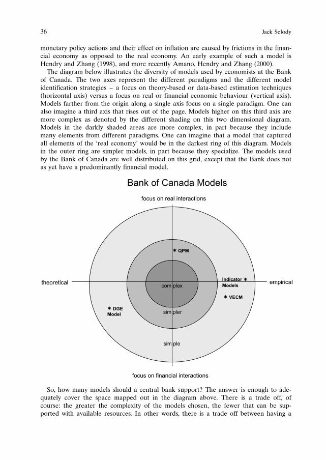
monetary policy actions and their effect on inflation are caused by frictions in the finan-cial economy as opposed to the real economy. An early example of such a model isHendry and Zhang (1998), and more recently Amano, Hendry and Zhang (2000).The diagram below illustrates the diversity of models used by economists at the Bank
of Canada. The two axes represent the different paradigms and the different modelidentification strategies – a focus on theory-based or data-based estimation techniques(horizontal axis) versus a focus on real or financial economic behaviour (vertical axis).Models farther from the origin along a single axis focus on a single paradigm. One canalso imagine a third axis that rises out of the page. Models higher on this third axis aremore complex as denoted by the different shading on this two dimensional diagram.Models in the darkly shaded areas are more complex, in part because they includemany elements from different paradigms. One can imagine that a model that capturedall elements of the ‘real economy’ would be in the darkest ring of this diagram. Modelsin the outer ring are simpler models, in part because they specialize. The models usedby the Bank of Canada are well distributed on this grid, except that the Bank does notas yet have a predominantly financial model.
So, how many models should a central bank support? The answer is enough to ade-quately cover the space mapped out in the diagram above. There is a trade off, ofcourse: the greater the complexity of the models chosen, the fewer that can be sup-ported with available resources. In other words, there is a trade off between having a
36 Jack Selody
���� �� ����� ���
�� ���
���� �� ���� �����������
��������������������
���� �� ��������� �����������
������� ��
������
�� ���
�����
�� ����
com plex
sim pler
sim ple

greater number of points in the outer ring of the space, or fewer points near the centreof the space. At the Bank of Canada, we have chosen to support a greater number ofsimpler models.
2.3. Should each paradigm be supported by a separate group of researchers?
When a central bank decides to support multiple paradigms, how should it organize itsmodellers, researchers and policy analysts to maximize their effectiveness? Is it betterto develop and maintain models in a cooperative or competitive environment? A coop-erative environment is more likely to be attained if all paradigms are developed andmaintained by a single set of economists. A competitive environment is more likely toevolve if different models are developed and supported by different groups.The advantage of a cooperative environment for model development and mainte-
nance is that it encourages policy researchers to arrive at a consensus of how best tomodel an economic phenomenon. It also encourages the use of the same elements indifferent models – for example, the same concepts and measures of energy priceswould likely appear in both real and financial models. The disadvantage of using simi-lar elements in different models is that sometimes such elements are themselves uncer-tain and so it is sometimes useful to use a variety of methodologies to construct a givenconcept.An environment which has different groups supporting different models is more
likely to expose the weaknesses of the competing paradigms as each modelling group islikely to work towards demonstrating the superiority of its paradigm. Such competitioncould also lead to more rigorous testing of competing models. For example, researchersworking on the money-growth paradigm at the Bank of Canada work in a differentdepartment from those working on the output-gap paradigm. One of the features thatdistinguishes the money and output-gap paradigms is the micro behaviour of price set-ters: price setters in the money paradigm are presumed to look predominantly at cashflow when setting prices, whereas price setters in the output-gap paradigm are pre-sumed to look predominantly at inventory levels or at the excess demand for theirparticular service. A competitive environment encourages researchers to test these com-peting hypotheses in order to demonstrate the superiority of their paradigm. The disad-vantage of such competition is that it highlights the differences between paradigms,rather than the similarities, which may give outside observers the mistaken impressionthat researchers at the central bank are more uncertain about the transmission mechan-ism than is in fact the case.The best environment for conducting policy analysis is one that emphasizes the posi-
tive elements of both the competitive and cooperative environments while playingdown, or finding ways to mute, the negative elements. There is no unique way ofachieving this objective. At the Bank of Canada we have adopted what is essentially acompetitive environment while encouraging economists to recognize the value of amultiple paradigms approach, which encourages cooperation between competinggroups. The separation of the financial and real departments is motivated in part by adesire to keep the policy advice generated by the two paradigms as independent aspossible. It also recognizes the fact that the Bank of Canada has some responsibility forcollecting financial data but not real data. Also, the output-gap paradigm is the domi-nant paradigm at the Bank of Canada, and therefore the real economic department is
Uncertainty and multiple perspectives 37
more oriented towards the production of forecasts and current analysis than is the de-partment that maintains the money paradigm, which is more oriented towards conduct-ing research aimed at developing the financial paradigm.On the other hand, both departments use multiple identification strategies for
building the models that represent their paradigm. These include pure time seriesindicator models, structural vector auto-regressive models, ad hoc decision-rule modelsbased on concepts such as the IS curve and the Phillips curve, and choice theoreticdynamic general equilibrium models. There is much cooperation between the depart-ments on developing model identification techniques. Thus, technical advances inmodelling are disseminated rapidly to researchers and policy analysts working in bothdepartments.
2.4. Does it make sense to build a model that encompasses all relevant paradigms?
This issue is about a trade off between consistency and completeness. Consistency in amacro economic model means that the behaviour attributed to an economic agent inone part of the model is derived from the same choice theory that determines thebehaviour of that agent in another part of the model. It also means that all agents actin an optimal manner in all their interactions in the model, basing their decisions on aconsistent set of information. And, it means that budget constraints – on both incomeand wealth – are respected in the model. The current state of economics is such that itis impossible to build a single macro economic model that encompasses all aspects ofthe transmission mechanism in a consistent manner. That is, it is currently impossible tobuild a macro economic model that is both consistent and complete.The multiple paradigm approach to policy analysis advocates putting consistency
ahead of completeness within a single macro economic model. Completeness is thenobtained by building an collection of consistent but separate macro economic models.Once such a collection of macro economic models has been amassed, it is natural toask whether there is a need for an additional, more pragmatic model that sacrificesconsistency for completeness – that is, a model that captures all relevant aspects of thetransmission mechanism even though such a model would not be fully consistent inter-nally.The main argument against maintaining a pragmatic model is that it would be hard,
if not impossible, to interpret the policy advice generated from such a model. The rea-son interpretation is difficult is that such a model would not be a good representationof any paradigm because of its lack of internal consistency. As an example, consider amodel that would incorporate both the output-gap and the money paradigms. The out-put-gap paradigm explains the transmission mechanism in a complete and consistentway using mostly ‘real’ variables. The money paradigm explains the transmission me-chanism in a complete and consistent way using mostly financial variables. To mergethe two paradigms, the internal consistency of both the real and financial behaviours ofagents in the model would have to be compromised, and the resulting model would notbe entirely representative of either paradigm. Thus, the policy advice derived from themodel would be based on behaviour that was inconsistent with both paradigms.An additional argument against a pragmatic model is that it would have to ignore
important details of both paradigms in order to remain tractable. There do exist, forexample, simple IS-LM type models that incorporate both real and financial elements.
38 Jack Selody
However, such models do not describe the monetary transmission mechanism in en-ough detail to satisfy most policy analysts. And, obtaining model consistency in a largermore detailed model is currently impossible.
3. Distillation of advice issues
3.1. Which policy path to choose?
When policy advisers use different models to generate multiple paths for the policyinstrument, most likely they will be asked to recommend a best path. Even when thechoice between alternative paths is left to the policy makers, it is likely that policyadvisors will be asked for analysis on how to choose between competing paths. So, howmight policy advisors choose a single recommended path?The most straightforward way of constructing a single recommended path is to com-
bine alternative paths using a fixed weighting scheme. The weights could mirror therelative accuracy of the different models in predicting inflation two years into the fu-ture, for example. The setting for the policy instrument at each point along the recom-mended path would then be a weighted average of the settings at each point along thepaths from the alternative models.The problem with this approach is that the resulting ‘best’ path will be inconsistent
with the individual paths from all models. It may therefore be difficult to explain anddefend the policy actions that would result if policy makers followed this ‘compromise’path. This will not be a problem when the policy paths from the alternative models aresimilar. But, in this case, choosing between policy paths is not an issue. A weighted, orcompromise, path is more likely to be a problem when the recommendations from thealternative models diverge considerably. In this case, policy in one of the model haslikely reacted to an economic event or feature of the transmission mechanism that isnot present in the other models. Moreover, in the case where such events happen infre-quently, the weight that should be applied to this event or feature is unlikely to bedirectly related to the average of the historical forecast performance of the model inwhich it resides, and therefore weighting schemes derived from the average relativeforecast performance over the historical sample are unlikely to be appropriate.An alternative approach to choosing the recommended path is to identify one of the
models as the dominant model and to generate the policy path from this model using ageneralized Taylor rule that is robust in the sense that it does not produce bad out-comes in any of the alternative models. The dominant model could be chosen by aconsensus of the policy makers, advisors, and researchers within the institution. Re-search on alternative models would continue. The policy advice from the alternativemodels would still be presented to policy makers as it would help them understand thelimitations of the policy advice coming from the dominant model.2
One disadvantage of this approach is that the dominant model excludes elements ofthe transmission mechanism that can be important from time to time, and the general-ized Taylor rule can produce advice that is far from optimal under some conditions.This means that using the dominant model with a generalized Taylor rule is inappropriate
Uncertainty and multiple perspectives 39
2 This approach is similar, although not identical, to the approach followed at the Bank of Ca-nada. See Longworth and Freedman (2000) for a complete description of the elements and pro-cesses that constitute the conduct of monetary policy at the Bank of Canada.

in some, albeit unusual, circumstances. In particular, the policy advice from the dominantmodel might be quite inappropriate in large episodic events, such as credit crunchesand booms, since the dominant model has not been constructed to explain such events.In these cases it is necessary for policy advisors, or the policy makers themselves, toapply judgement to the advice coming from the dominant model. However, given insti-tutional inertia, it is possible that the inappropriate nature of the policy advice comingfrom the dominant model may not be appreciated rapidly enough to formulate andapply the necessary judgement in a timely manner.To avoid contributing to institutional inertia, it is important that policy makers take
the alternative models seriously. When advice from alternative models is not taken ser-iously it indicates to researchers that further research on alternative paradigms is unli-kely to be appreciated, and so it will become increasingly difficult to develop and main-tain alternative models. And, if the alternative models are not continually maintained, itmay be difficult for policy advisors to recommend that more weight be given to analternative model in those cases where economic circumstances warrant such advice. Asan incentive to maintain the alternative models, it is useful to give them a formal rolein the policy discussion.One way of giving the alternative models a formal role in conditioning the recom-
mended path for the policy instrument is to identify explicitly the conditions underwhich the policy recommendation from the dominant model is unlikely to be appro-priate. For example, the policy advice coming from an output-gap model is unlikely tobe optimal in the face of a credit crunch or financial market crisis because it does nottake account of the financial aspects of the transmission mechanism. In cases wheresuch economic conditions arose, or in which the economy started behaving in ways notexplained by the dominant model, optimal advice from alternative models could beapplied at the margin. This optimal advice could come from using a generalized Taylorrule in the alternative model, or it could be derived optimally from the hypotheticalsocial welfare function of the hypothetical monetary authority in the alternative model.
3.2. What process should be used to present advice to policy makers?
Good information leads to better decisions. This means that a full and balanced discus-sion and debate of policy issues prior to a policy decision is likely to result in betterpolicy. Thus, one of the goals of the process by which policy advice is presented topolicy makers is to encourage discussion and debate of the issues. Looking at the issuesusing multiple paradigms facilitates such discussion and debate.Essentially, there are five groups of people who are critical to a full and complete
policy debate. (1) The model builders and policy analysts who conduct research andbuild macro economic models such that they have first hand knowledge of the strengthsand weaknesses of the models that are used in the central bank. This group of peopletend to have great technical expertise. (2) Policy advisors who understand the modelsand the context in which they are used. (3) Policy makers who understand the contextwithin which policy is implemented and whose judgement forms the basis of the policydecision. (4) Outside technical experts who understand the strength and weaknesses ofthe models being used, but who have not built or used the models in question andtherefore are likely to have a different perspective from those inside the central bank.(5) Members of the general public who will be affected by the policy decision.
40 Jack Selody

Groups (1) through (3) tend to participate in the internal policy debate. Groups (3)through (5) tend to participate in the external policy debate. Both debates are impor-tant to the policy decision. This said, the remainder of this section is devoted to pro-cesses that make the internal policy debate most effective.Given the different levels of technical expertise of the three groups involved in the
internal policy debate, it is logical to take a sequential approach to the internal debate.The benefit of a sequential approach is that it is efficient in that technical modellingissues will be debated separately from issues that cannot be adequately modelled. Ofcourse, the policy decision makers must be aware of all important issues, technical ornot, if their decisions are to be based on all available information.If policy makers are to have full information, they should be presented with the
information from all models. There is no unique way to ensure that policy makersobtain all relevant information. If the policy makers themselves have a good under-standing of modelling technology then it is probably best to present the advice from thealternative models separately and directly to the policy makers. This is the approachtaken at the Bank of Canada. Alternatively, if the policy makers have a strong desire tofocus the internal debate around a single dominant paradigm, the advice from the mul-tiple models can be reconciled by policy advisors before being presented for discussionto policy makers. In this case, the risks identified by the alternative models should behighlighted, but the advice coming from the alternative models will have been incorpo-rated into the advice from the dominant model at the margin and therefore need notbe shown separately. Where the desire to have a single dominant paradigm is verystrong, it may be sufficient to conduct research into the alternative paradigm and to usethe results of this research to improve the dominant model at the margin. In this case,the alternative model does not become fully articulated, nor is it used to produce alter-native policy advice, but research into the paradigm is used to identify issues that canbe explored within the dominant paradigm.An example of a process that results in full information being given to the policy
makers would be one that gave separate policy advice from alternative models directlyto policy makers. The first stage of debate would be technical discussions of the modelsused to represent each paradigm. Such a discussion would no doubt concentrate on thelatest modifications to the models that would have resulted from on-going research intothe paradigm. Such modifications would help the users of each model better interpretrecent events consistent with their separate paradigm.The second stage of the debate would start after the models had generated an array
of possible paths for the policy instruments conditional on different future values fortheir exogenous variables and conditional on different assumptions about the economicbehaviours included in the model. This debate would involve the policy advisors who,after a discussion with the technical experts, would choose what they considered to bethe most reasonable policy path from each paradigm to present to the policy makers.This need not be the optimal path from each model as the policy advisors may want toexercise judgement at this point. For example, the policy advisors may think that thecurrent economic environment is particularly uncertain and so emphasize robustnessover optimality in choosing the path. Again, this discussion would take place separatelyfor each paradigm to keep the advice coming from the different models as independentas possible. At this stage, it would sometimes be useful to construct a policy path thatcombines elements from both models. In this case there would be three proposed policy
Uncertainty and multiple perspectives 41

paths – the most reasonable path from the dominant model, the most reasonable pathfrom the alternative model, and a compromise policy path.It is these three paths, along with a discussion of how the paths were obtained, why
they were chosen, and perhaps some interesting alternative paths that were not chosen,that could be presented to the policy makers to support the third stage of the debate.This information could be augmented by scenarios that would highlight the risks asso-ciated with the assumptions used to generate the proposed policy paths and any contro-versial features of the model that were affecting the proposed policy paths. Policy ma-kers would then choose a single path for implementation based on this information,their own judgement about the future paths of exogenous variables, what emphasis toplace on the different models, as well as their own assessment of economic conditions.In choosing this path, the policy makers would have obtained all relevant informationfrom the competing models as well as from their advisers on how to interpret andcombine that information, judgement from their staff about the most likely paths of theexogenous variables driving the models, as well as judgement about what behavioursare currently dominating the transmission mechanism. The chosen path would then becommunicated back to the model builders and policy analysts so that it could form thebasis of the next policy exercise. Of course, in practice, the chosen path would be fol-lowed only for a single quarter as the policy exercise would be repeated each quarteras new information became available, including information on the forecast accuracy ofthe different models.
4. Communication issues
Explaining monetary policy decisions to the public can be difficult even in the best ofcircumstances. The relationship between interest rates and inflation is complicated anddifficult to explain. There are many elements of the monetary transmission mechanismthat are not well understood. The lags between interest rates and inflation are long andvariable. The conditional nature of forecasts and policy statements is often difficult formarket participants, journalists and the public to appreciate fully. And few commenta-tors fully appreciate the degree of uncertainty that affects economic data, theory, andthe policy decision. Given such conditions, it might seem that explaining multiple para-digms – that is, explaining that there are multiple ways of viewing the transmissionmechanism – would be an unnecessary complication that could hinder good publiccommunication.Yet many central banks already use more than one paradigm, at least implicitly, to
communicate their policy decisions. In public commentary, many central bankers referto inflation as a monetary phenomenon even though their main macro economic modeldoes not reflect this view. In effect, the paradigm that central bankers use for commu-nication purposes is necessarily less precise and consistent than the models they use forpolicy decisions. One reason for this disconnect is that many of the elements that condi-tion the policy decision are not found in a single macro economic model. Thus, centralbankers take a pragmatic approach to communicating their policy decisions by talkingabout a variety of economic indicators, influences, and economic behaviours.Even though many central banks take a pragmatic, multiple paradigm approach to
communicating their policy decisions, not all central banks formalize this to the sameextent. Some central banks maintain a formal distinction between the two paradigms in
42 Jack Selody

public such as the European Central Bank with its two pillars approach to communicat-ing monetary policy. This approach encourages specialized communication in the con-text of both paradigms that should help support the public debate about policy issuesand contribute to better policy decisions. Such an approach also has the potential toprovide the greatest consistency between the discussions that take place within the cen-tral bank and those that take place outside the central bank. Other central banks takea less formal approach to communicating multiple paradigms, preferring to present thedifferent elements that go into a policy decision in a consistent way, even though theelements have not been reconciled within a single macro economic model. Such anapproach may make it easier to understand the policy decision, but it does less to high-light the different perspectives that arise from the multiple paradigm approach. Eitherapproach can support effective communication, and both approaches can contribute tothe public policy debate if the communication with the public is open and transparent.The Bank of Canada takes a pragmatic approach to communicating its policy deci-
sions to the public, even though the policy analysis behind the decisions is the productof separate paradigms. That is, the analysis behind monetary policy decisions is commu-nicated to the public as if it were the product of a hypothetical complete macro eco-nomic model that incorporates all relevant economic behaviour, even though a formalmathematical model with such characteristics does not exist, nor can it be constructedtoday. For example, in the Monetary Policy Report there is a through discussion ofmonetary aggregates and what they suggest about inflation and output growth, as wellas a discussion of aggregate demand and supply imbalances. Such pragmatism – whichalso characterizes the way most central banks communicate – is flexible enough tocommunicate all the analysis behind policy decisions.A pragmatic approach to communication does not discourage the publication of tech-
nical documents that describe the different macro economic models used by economistsat the central bank. As is the case at the Bank of Canada, the authors of such docu-ments should be encouraged to make explicit reference to the paradigm behind themodel, and to discuss the limitations of that paradigm. Research that compares therelative performance of the paradigms should also be produced. Being explicit aboutmultiple paradigms in technical documents, while taking a pragmatic approach to com-munication in more accessible publications, allows communication to different audi-ences in a way that maximizes their understanding of the policy decision, and thusenhances their ability to contribute to the policy debate.
5. Summary
A multiple paradigm approach to monetary policy advice can lead to better advice be-cause it adds robustness to that advice. Good monetary policy advice is both near optimalwithin a single model and robust across models. Different models emphasize differentaspects or interpretations of the monetary policy transmission mechanism and, therefore,advice that is appropriate across multiple models should be less sensitive to errors inanalysis that arise when knowledge of the transmission mechanism is uncertain.This paper discussed issues that arise when implementing a multiple paradigm ap-
proach to monetary policy advice. The discussion identified three broad sets of issues.The first set of issues involved the type of models that might be built to represent the
different paradigms. Given limited research and analytic resources within a central
Uncertainty and multiple perspectives 43

bank, there is a trade-off between the number of paradigms that can be supported by acentral bank and the complexity of the models. In addition, different paradigms shouldbe as distinct as possible to avoid duplication and redundancy. Consistent with thisapproach, the Bank of Canada supports two paradigms and two approaches to modelidentification – models that focus on real or financial interactions when explaining in-flation, and empirical or theoretical approaches to model identification.One of the main values that a macro economic model brings to the policy debate is
internal consistency between the concepts and behaviours that appear in the model. Topreserve consistency, each model should be maintained separately from the other mod-els in order to avoid the introduction of extraneous concepts and incongruous beha-viours. This would suggest that it is best that each paradigm be maintained by a sepa-rate group of economic researchers and policy analysts, and that each group maintainmultiple models to represent their paradigm. This said, these groups should communi-cate extensively to ensure that advances in modelling methodology are disseminatedrapidly.Maintaining consistency also means that no single model or paradigm can capture all
aspects of the monetary transmission mechanism because knowledge of the trans-mission mechanism is incomplete, even though our knowledge is based on a wide rangeof information and interpretative tools. Introducing pragmatism into a single macroeconomic model would cloud the interpretation of the output of the model, whichwould reduce the usefulness of the policy advice generated from the model.Monetary policy advice is better when it is formed in an environment of vigorous
and open debate. The process by which policy advice reaches the policy decision ma-kers is therefore as important as the models that are used to generate policy advice.There is no best way of combining the information from multiple models, be it at theresearch stage, the policy analysis stage, or the policy decision stage. Whatever processis adopted, it should aim at encouraging a vigorous and open debate of the policyissues at all stages. The process should also be structured to allow broad participationin the debate without wasting too much time. This would suggest that a technical de-bate about the merits of each paradigm should take place separately from the debateabout the recommended policy outcome. A technical debate should be conducted foreach model separately to ensure that the advice being generated by one model is asindependent as possible from that of the other models. The debate about the recom-mended policy outcome should be based on the advice coming from the alternativemodels separately in order to ensure that all relevant information is available to thepolicy decision makers.The external policy debate on monetary policy is as important to good monetary
policy decisions as is the internal monetary policy debate. This means that good com-munication of the reasons for a monetary policy decision and outside scrutiny of themodels, research and analysis that go into the policy decision are important elements ofthe process that generates policy advice. Information aimed at the external audienceshould be clear and concise in order to enhance understanding. For the non-expertaudience this may be achieved either by a pragmatic approach to communicating policydecisions or by maintaining the distinction between paradigms in communication to thepublic. The expert external audience, however, is aware of the uncertainty that sur-rounds knowledge of the monetary transmission mechanism, and so for this audience itis likely better to be clear about the distinction between paradigms by offering a formal
44 Jack Selody

explanation of the models used to represent each paradigm and by publishing the re-sults of tests of the relative performance of these models. Clear and effective externalcommunication will lead to better monetary policy decisions by helping experts and thegeneral public participate in the policy debate.
References
Adam, Charleen and Scott Hendry 2000 “The M1-VECM: Some Extensions and Applications”Money, Monetary Policy and Transmission Mechanisms proceedings from a conference held atthe Bank of Canada.
Amano, Bob, Scott Hendry and Guang-Jia Zhang 2000 “Financial Intermediation, Beliefs and theTransmission Mechanism” Money, Monetary Policy and Transmission Mechanisms, proceedingsfrom a conference held at the Bank of Canada.
Brainard, William C. 1967 “Uncertainty and the Effectiveness of Policy” American EconomicReview Papers and Proceedings, 57(2).
Engert, Walter and Jack Selody 1998 “Uncertainty and Multiple Paradigms of the TransmissionMechanism” Bank of Canada Working Paper 98-7.
Hendry, Scott and Guang-Jia Zhang 1998 “Liquidity Effects and Market Frictions” Bank of Cana-da Working Paper 98-11.
Longworth, David and Charles Freedman 2000 “Models, Projections, and the Conduct of Policy atthe Bank of Canada” Stabilization and Monetary Policy: The International Evidence, presentedat a conference organized by Banco de Mexico.
Muller, P. 1992 “The Information Content of Financial Aggregates During the 1990s” MonetarySeminar 90, proceedings of a seminar sponsored by the Bank of Canada.
Sargent, T.J. 1999 “Comment on ‘Policy Rules for Open Economies’ ” in John Taylor (ed.) Mone-tary Policy Rules University of Chicago Press.
Srour, Gabriel 1999 “Inflation Targeting under Uncertainty” Bank of Canada Technical Report 85.Taylor, John 1993 “Discretion versus Policy Rules in Practice” Carnegie-Rochester Series on Public
Policy North Holland 39, pp. 195–214.Taylor, John 1999 “An Historical Analysis of Monetary Policy Rules” in John Taylor (ed.) Mone-
tary Policy Rules University of Chicago Press.Tkacz, Greg and Sarah Hu 1999 “Forecasting GDP Growth using Artificial Neural Networks”
Bank of Canada Working Paper 99-3.
Uncertainty and multiple perspectives 45

1. The new policy approach of the Swiss National Bankand the role of money
1.1. New approach based on inflation forecast
At the end of 1999, the Swiss National Bank (SNB) modified its monetary policy ap-proach. It abandoned monetary targeting in favour of a policy concept based on aninflation forecast. The SNB’s new approach entails three elements.1
First, the SNB announced a definition of price stability, expressed in terms of theheadline CPI. It defines price stability in the same manner as the European CentralBank (ECB). According to the SNB, price stability equals a CPI inflation rate of lessthan 2 percent per year. Although the lower bound of the range in the inflation rateconsistent with price stability remains undefined, the SNB made it clear that it willendeavour to prevent deflation, i.e., a decline in the CPI.Second, the SNB publishes an inflation forecast twice a year. The inflation forecast,
which is announced at press conferences in June and December, is offered for threeyears ahead. The three-year forecasting period takes account of the long time lag in theeffects of Swiss monetary policy. In Switzerland, as many as three years tend to elapseuntil a change in monetary policy fully affects the inflation rate. In addition, the SNBprovides a forecast of real growth in the following two years.The SNB compares its inflation forecast with its definition of price stability. If the
SNB expects the inflation rate to move outside the price-stability range, it must contem-plate adjusting monetary policy. However, the SNB does not alter monetary policy me-chanically in response to deviations in the inflation rate from the price-stability range.It is mainly concerned about keeping the inflation trend within this range. The SNB isprepared to tolerate temporary deviations from the price-stability range, caused by suchfactors as fluctuations in energy prices and exchange rates, as well as changes in indir-ect taxes. For example, due to the recent sharp increase in the oil price, inflation mayrise temporarily above the threshold of 2 percent in 2001 or 2002. Yet, the SNB has
The role of M3 in the policy analysisof the Swiss National Bank*
Thomas J. Jordan, Michel Peytrignet and Georg Rich
Swiss National Bank
* Paper presented at the Central Bank Workshop on Monetary Analysis, organised by the Eur-opean Central Bank, Frankfurt a/M, November 20 and 21, 2000. Helpful comments by AnnickBruggeman, Vincent Perilleux, Marcel Savioz, Lars Svensson and the participants of the Workshopare gratefully acknowledged.
1 See Meyer (2000) and Rich (2000) for more detailed discussions of the new approach.

emphasised that it does not intend to tighten monetary policy further, despite the ex-pected departure from the price-stability range. In the SNB’s view, attempts to keep theinflation rate within the price-stability range at all times would unnecessarily exacerbatefluctuations in Swiss output and employment. Because of its focus on the inflationtrend and on headline inflation, the SNB is reluctant to treat its definition of pricestability as a binding inflation target even though its policy approach is akin to inflationtargeting as pursued by the Reserve Bank of New Zealand, the Bank of Canada, theBank of England, the Sveriges Riksbank and other central banks.The third element in the SNB’s new approach involves modifications to its opera-
tional procedures. Before the end of 1999, the SNB translated its policy intentions intooperational targets for bank reserves. Since the beginning of 2000, it has fixed an opera-tional target band for the three-month Libor for Swiss francs, with the bandwidthamounting to 100 basis points. The SNB does not control the three-month Libor di-rectly, but indirectly by way of changes in the overnight-lending rate.
1.2. Importance of money and other policy indicators
The SNB did not entirely discard the approach followed before the end of 1999 andretained important ingredients of monetary targeting in its new monetary policy con-cept. At various occasions, the SNB stressed that it continues to monitor two sets ofindicators providing leading information on future price developments in addition tousing econometric forecasting models. The first set of indicators is useful for forecastingshort-run price developments, i.e., over a horizon of up to 1 =–2 years. It includes var-ious indicators on the cyclical state of the economy, notably the output gap and supplyand demand conditions in the labour market, as well as the real exchange rate of theSwiss franc. The second set of indicators comprises the monetary aggregates, whichprovide useful leading information on long-run price developments. A substantial bodyof evidence suggests that the growth in the Swiss money stock M3, in particular, isstably related to inflation and output growth, and serves as a key determinant of infla-tion in the long run (Peytrignet, 1996, 1999; Peytrignet and Stahel, 1998). Both sets ofindicators are used together with the forecasts from various econometric models toproduce a broadly based consensus inflation forecast, which now forms the centre stageof Swiss monetary policy.In addition to being important inputs to the consensus forecast, the SNB monitors
these policy indicators for two other reasons. First, while the SNB tends to adjustmonetary policy, if necessary, upon announcing a new inflation forecast, it cannotcontent itself with reviewing its policy course only twice a year. Shocks threatening tojeopardise price stability may occur at any time. Therefore, the SNB must be preparedto act whenever shocks call for a change in monetary policy. Under monetary targeting,the SNB already reviewed its policy course at quarterly intervals and, if necessary,more often. It has maintained this practice under the new regime although two ofthese quarterly reviews do not result in the publication of a new inflation forecast.Moreover, the SNB is willing to change the target band for the three-month Libor inbetween its quarterly policy reviews, should there be a need for such actions. If apolicy change is not accompanied by the publication of a new inflation forecast, theSNB justifies its policy measure by referring to the leading indicators of inflation thatit monitors regularly.
48 Thomas J. Jordan, Michel Peytrignet and Georg Rich

A second – and even more important – reason for monitoring policy indicators liesin the SNB’s accountability to the public. The public must be able to judge whether theSNB’s policy stance is appropriate for achieving the ultimate objective of price stability.Under the approach followed before the end of 1999, the intermediate monetary targetprovided the main yardstick for assessing Swiss monetary policy. According to Svensson(1997; 1999), central banks following inflation targeting or similar approaches shouldtreat their inflation forecast as an intermediate target. In this case, the central bankproduces a forecast of inflation conditional upon various paths for the policy instru-ment. The policy makers in turn select the instrument path that generates an inflationforecast conforming to the inflation target.2 If the inflation-forecast target is to be effec-tive in enforcing accountability, the central bank must not only publish its inflation fore-cast, but also explain to the public how it arrived at its prediction. Otherwise, the publicwill be unable to judge whether the operational framework chosen by the central bankis suitable for achieving the inflation target.3
The main difficulty with this approach lies in the subjective nature of inflation fore-casts. There is an important difference between intermediate targets for a monetaryaggregate and an inflation forecast. The money stock is a variable that can be mea-sured objectively, while the inflation forecast rests on the central bank’s subjectiveviews about the future. If the central bank is under strong political pressure to pursueobjectives that are likely to be at variance with price stability in the long run, it mayproduce inflation forecasts biased in favour of the politicians’ preferences. This may beparticularly true of forecasts for inflation two or three years ahead. A willingness tomonitor the development of monetary aggregates may serve as a remedy against biasedinflation forecasts provided these aggregates are reliable leading indicators of inflation,as is the case in Switzerland.4 Thus, monitoring indicators such as the monetary aggre-gates may improve policy performance in two ways: It may help the central bank inelucidating its policy analysis and in communicating its inflation forecasts to the public.Furthermore, it may discourage the central bank from publishing biased inflation fore-casts.Although the leading-indicator role of Swiss monetary aggregates is uncontested, it is
difficult to explain to the public how they enter into the monetary policy decisions.When the SNB developed its new policy framework, it discussed the possibility ofadopting the two-pillar strategy of the ECB. A two-pillar strategy would have allowedthe SNB simultaneously to shift its policy focus to inflation forecasts and to retain themonetary aggregates as important policy indicators. After much reflection, the SNBdecided against a two-pillar strategy. Instead, it emphasised that it would base its policydecisions mainly on an inflation forecast. The money stock M3, along with the other
The role of M3 in the policy analysis of the Swiss National Bank 49
2 Svensson (1999, pp. 623–630) actually suggests more complex procedures, under which thecentral bank engages in “flexible” inflation targeting, i.e., its loss function comprises an output-gaptarget, in addition to an inflation target. As indicated above, the SNB takes account of output insetting monetary policy.
3 Informing the public about the intricacies of a conditional inflation forecast is a difficult taskindeed. In our experience, even policy makers themselves are sometimes at a loss to grasp fullythe meaning of such forecasts.
4 Forecasts produced by the private sector may also help in detecting biases in central-bankforecasts. However, it is possible that private forecasters are swayed by the same political consid-erations as the central bank.

indicators mentioned above, would serve as important input into the inflation forecast.Moreover, monitoring M3 and other indicators would help the public to understand thereasoning behind the SNB’s forecast. These indicators would also be used to justifypolicy changes at times at which the SNB did not publish a new forecast.The SNB was concerned that – with a two-pillar strategy – it would reintroduce to
the new approach a problem that had plagued monetary targeting. Its concern derivedfrom the reference value for M3 growth, a key ingredient of the ECB’s strategy. TheSNB was reluctant to follow the example of the ECB and to fix a reference value forM3 growth. Such a reference value would have closely resembled the multi-year targetfor money growth that the SNB had set under the policy regime in operation beforethe end of 1999. The SNB did not wish to fix a multi-year target under a new guisebecause this target had created complex problems of signal extraction that are typicalfor monetary aggregates whose demand is highly sensitive to changes in interest rates.As we have shown elsewhere (Peytrignet, 1996, 1999; Rich, 1999, 2000), if money de-mand responds strongly to changes in interest rates, steady expansion in the moneysupply is unlikely to constitute an optimum policy strategy. In the case of Swiss M3, forexample, money growth should normally rise above and fall below its long-run averageduring cyclical contractions and expansions in economic activity respectively. Thus, ta-ken by themselves, the deviations in M3 growth from a long-run average or referencevalue may provide misleading information about the stance of monetary policy. Duringthe contraction phase of the business cycle, a positive deviation may indicate that thepolicy stance is in sympathy with price stability. During the expansion phase, by con-trast, a positive deviation of the same size may point to the SNB following an inflation-ary policy course.5 Observers of Swiss monetary policy frequently believe that a me-chanical relationship exists between money growth and inflation. Fixing a referencevalue for M3 growth might have reinforced these misconceived views about the linkbetween money growth and inflation.In the following, we attempt to resolve the signal-extraction problem just described.
In Section 2 we develop an empirical procedure designed to extract useful informationon future inflation from the Swiss aggregate M3, while Section 3 offers conclusions.
2. The empirical importance of M3 as an information variable
The procedure used for extracting information rests on the observation that the demandfor Swiss M3 is stable in the long run and that the variables entering into the moneydemand function are therefore cointegrated. This allows us to explore the predictivepower of two measures of M3.6 The first measure consists of the growth in the season-ally-adjusted money stock M3, as recorded in Swiss monetary statistics. It will be called“money growth” in the subsequent analysis. The second measure will be called “excessmoney” and equals the error term in the cointegrating relation, i.e., the logarithmicdifference between the seasonally adjusted recorded levels of M3 and the correspond-ing trend values derived from the cointegrating relation.
50 Thomas J. Jordan, Michel Peytrignet and Georg Rich
5 The same conclusion holds for the monetary base, the SNB’s intermediate target variableuntil the end of 1999, and the aggregates M1 and M2. Of course, the SNB was aware of thisproblem when it targeted money.
6 Swiss M3 consists of Swiss-franc-denominated currency, sight and other transactions deposits,as well as time and savings deposits, in the hands of domestic nonbank residents.

The measures of M3 are used to forecast both the time path of future inflation andcumulative price increases over periods exceeding one year. Moreover, the predictivepower of these measures is determined for forecasting horizons of varying length. Inthis paper, we will consider only in-sample evidence because the available data seriesare relatively short and thus unsuitable for computing meaningful out-of-sample results.Nevertheless, in-sample results provide interesting evidence on the robustness of theinformation contained in M3 over a longer period of time.
2.1. Money growth and excess money
Studies on money demand in Switzerland, using a variety of approaches, lead to theconclusion that the aggregate M3 is cointegrated with the price level, output, and thelong-term interest rate. Money demand functions for M3 consisting of these variablesare therefore stable in the long run. Recent examples of such studies are Baltensperger,Jordan and Savioz (2000), Peytrignet (1996), and Peytrignet and Stahel (1998). For thepurpose of this paper, we do not estimate the cointegrating vector of the demand forM3. Rather, we calibrate the long-run demand for M3 by drawing on the results fromexisting studies. We are forced to rely on calibration because subsequently we will userolling estimation to forecast inflation. The sample size is not sufficiently large to allowrolling estimation to be applied to the cointegrating relation too. Our calibrated long-run demand for M3 is
m3t ¼ �1:65þ 1:0 � pt þ 1:3 � qt � 0:05 � Rt þ ect ; ð1Þ
where m3 denotes M3, p the GDP-deflator, q real GDP and R the long-term interestrate (the yield of bonds issued by the Swiss Confederation with a maturity of tenyears), while t is a time index. All the variables except the long-term interest rate areexpressed in logs. The elasticities appearing in Eq. (1) are in line with economic theory.The non-unit income elasticity of 1.3 can be explained by the fact that M3 is used notonly for transaction purposes but also for the accumulation of wealth. The elasticity ofM3 with respect to income as a proxy of wealth is clearly higher than one.This long-run money demand equation allows us to compute excess money in the
economy, equalling the error correction term ec or the difference between the actuallevel of M3 and the value derived from Eq. (1), given the actual levels of prices, outputand the interest rate. The empirical analysis covers the period from the first quarter of1975 to the second quarter of 2000. Panel A of Figure 1 shows the evolution of excessmoney, expressed in percent of the equilibrium level of M3, over the sample period.From this figure it can be seen that over long periods of time, M3 fluctuated stronglyabout the equilibrium path explained by Eq. (1). Panel B of Figure 1 shows the annualgrowth of M3. As a reference, annual CPI-inflation is reported in Panel C of Figure 1.Since the demand for M3 is cointegrated, excess money or the ec term – in addition tomoney growth – should potentially be an exploitable indicator of future inflationarypressure.7 In the following, we analyse to what extent money growth and excess money– alone or together – provide information on future inflation in Switzerland.
The role of M3 in the policy analysis of the Swiss National Bank 51
7 Baltensperger, Jordan, and Savioz (2000) found that prices are not weakly exogenous to theerror correction term. Thus, they found Granger causality running from M3 to prices.
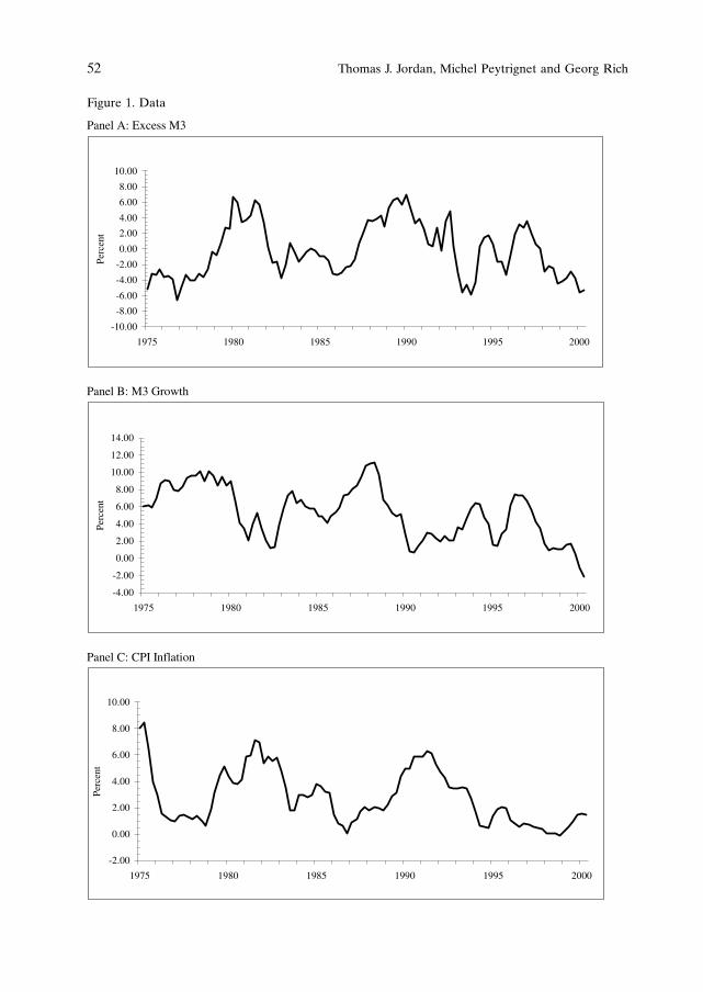
52 Thomas J. Jordan, Michel Peytrignet and Georg Rich
Panel A: Excess M3
Panel B: M3 Growth
Panel C: CPI Inflation
-4.00
-2.00
0.00
2.00
4.00
6.00
8.00
10.00
12.00
14.00
1975 1980 1985 1990 1995 2000
Perc
ent
-10.00
-8.00
-6.00
-4.00
-2.00
0.00
2.00
4.00
6.00
8.00
10.00
1975 1980 1985 1990 1995 2000
Perc
ent
-2.00
0.00
2.00
4.00
6.00
8.00
10.00
1975 1980 1985 1990 1995 2000
Perc
ent
Figure 1. Data

2.2. Some evidence from correlations
In this section, we search for the maximum correlation over different forecastinghorizons k between money growth and excess money, on the one hand, and inflationon the other. Inflation is defined as the change in consumer prices over the preced-ing four quarters, i.e., D4pct ¼ pct � pct�4. Money growth in measured analogously asD4m3t ¼ m3t �m3t�4. Thus, we consider the correlation between D4m3t and D4pctþk
and between ect and D4pctþk. We focus on D4-differences because in Switzerlandmonetary policy decisions are based on percentage changes in economic data overthe preceding year, rather than on annualised quarterly growth rates. In order to getinformation on the link between money and inflation for different time periods, weestimate the correlations recursively by lengthening the sample period gradually. Thefirst sample used in the computations covers the period 1976 :4 to 1986 :4, the sec-ond the elongated period 1976 :4 to 1987 :1, and so on. We also check whether theresults change over time, by estimating the same correlations with a moving windowencompassing 52 observations. Thereby, the first window covers the period from1976 :4 to 1989 :3, the second window covers the period from 1977 :1 to 1989 :4, andso on.Figure 2 reports the results. The horizontal axis depicts the date of the last observa-
tion of the estimation sample. In Panel A of Figure 2, the regular thin line refers to therecursively estimated maximum correlation between money growth and inflation.Lengthening the sample period shows that the maximum correlation between moneygrowth and inflation remains relatively stable between 0.4 and 0.6. Note that if weestimate the correlation with a rolling window of 52 quarters (dashed thin line), themaximum correlation of money growth with inflation is much more volatile. In Panel Bof the same figure, we find that the maximum correlation occurs between lag k ¼ 11and lag k ¼ 17 provided the correlations are estimated recursively (regular thin line).Most of the time, the lag with the maximum correlation is 15 quarters. The lag of max-imum correlation with rolling window estimation (dashed thin line) differs only slightlyfrom the results of the recursive approach.Panel A of Figure 2 also exhibits the recursively estimated maximum correlation be-
tween excess money and inflation (regular bold line). As in the case of money growth,the maximum correlation varies little over time and is quite high (between 0.6 and0.75). As a matter of fact, it is even higher for excess money than for money growth. Ifestimated with rolling windows of 52 quarters (dashed bold line), the maximum correla-tion between excess money and inflation becomes slightly more volatile than underrecursive estimation. Panel B indicates that the maximum correlation with recursiveestimation always occurs at lag k ¼ 4 (regular bold line), i.e., much earlier than in thecase of money growth. With rolling window estimation, by contrast, the lag variesslightly (dashed bold line).This exercise provides first insights into the information content of M3. Changes in
money growth lead subsequent changes in inflation by long time spans. The maximumcorrelation between money growth and inflation is relatively high; however, it fluctu-ates if different time windows are considered. In addition to money growth, excessmoney also incorporates information. For excess money, the lag of maximum correla-tion is much shorter, but the maximum correlation is even higher than for moneygrowth. These results suggest that M3 indeed possesses predictive power for futureinflation. However, the analysis presented thus far is not complete. It is also necessary
The role of M3 in the policy analysis of the Swiss National Bank 53

54 Thomas J. Jordan, Michel Peytrignet and Georg Rich
Panel A: Maximum Correlation Between Money and Inflation
Panel B: Lag of Maximum Correlation Between Money and Inflation
0.2
0.3
0.4
0.5
0.6
0.7
0.8
0.9
1986 1987 1988 1989 1990 1991 1992 1993 1994 1995 1996 1997 1998 1999 2000 2001
Cor
rela
tion
Max. Corr. Betw. Exc. M3 & CPI Inflation: Rec. Estim. Max. Corr. Betw. M3 Grt & CPI Inflation: Rec. Estim.
Max. Corr. Betw. Exc. M3 & CPI Inflation: Rolling Estim. Max. Corr. Betw. M3 Grt & CPI Inflation: Rolling Estim.
End of Sample
0
2
4
6
8
10
12
14
16
18
20
1986 1987 1988 1989 1990 1991 1992 1993 1994 1995 1996 1997 1998 1999 2000 2001
Lag
Lag Betw. M3 Grt & CPI Inflation: Rec. Estim. Lag Betw. Exc. M3 & CPI Inflation: Rec. Estim.
Lag Betw. M3 Grt & CPI Inflation: Rolling Estim. Lag Betw. Exc. M3 & CPI Inflation: Rolling Estim.
End of Sample
Figure 2. Correlation Analysis

to examine the information content of money growth and excess money simultaneously.Moreover, we should not only consider the lag with the maximum correlation, but alsodetermine the information content for other forecasting horizons.
2.3. Goodness of fit of forecasting regressions
This section examines the information content of M3 for different forecasting horizonsand over different sample periods. We also compare the information content of moneygrowth with that of excess money. For this purpose, we use the indicator model
D4pctþk ¼ b0 þ b1D4pct þ b2D4m3t þ b3ect þ "t : ð2Þ
The dependent variable is annual consumer price inflation in time t þ k, where t is thecurrent period and k the forecasting horizon. The indicator variables comprise the cur-rent annual inflation rate, D4pct, the current annual growth rate of M3, D4m3t, and theerror correction term ect (excess money) in time t. The error correction term ect iscomputed according to Eq. (1). The forecast error "t follows a moving average processof order k� 1.8 We consider three forecasting horizons of one (k ¼ 4), two (k ¼ 8), andthree years (k ¼ 12) since these are the most relevant for monetary policy purposes.To determine the information content of M3, four specifications of Eq. (2) are used.
Specification (2I), which may be regarded as a “naive” benchmark forecast, only takesaccount of current inflation. In Specification (2II), money growth is added in order toassess its marginal information content. Specification (2III) allows us to examine themarginal information content of the error correction term. Finally, specification (2IV)includes both money growth and the error correction term in order to assess the fullinformation content of M3:
D4pctþk ¼ bI0 þ bI
1D4pct þ "It ð2IÞ
D4pctþk ¼ bII0 þ bII
1 D4pct þ bII2 D4m3t þ "IIt ð2IIÞ
D4pctþk ¼ bIII0 þ bIII
1 D4pct þ bIII3 ect þ "IIIt ð2IIIÞ
D4pctþk ¼ bIV0 þ bIV
1 D4pct þ bIV2 D4m3t þ bIV
3 ect þ "IVt ð2IVÞ
The adjusted coefficients of determination ( �RR2) shed light on the in-sample informationcontent of money growth and excess money. Money is a valuable indicator if it carriesinformation about future inflation not already contained in current inflation. Thus, ifmoney is a useful indicator, the regressions including money growth or excess moneyshould display a higher �RR2 than the benchmark equation.We also test whether the information content of money changes over time by apply-
ing rolling regression methods. Rolling estimation of Eq. (2) yields time series of theadjusted coefficient of determination �RR2 for different forecasting horizons k. The �RR2 forhorizon k ¼ 4 are computed as follows: Eq. (2) is estimated over the period from1976 :1 to 1988 :4, i.e., with 52 observations. The �RR2 of this regression is in turn saved as�RR21988: 4. Then, the estimation sample is shifted one period ahead and the equation is re-
estimated with data running from 1976 :2 to 1989 :1. The �RR2 of this regression is savedas �RR2
1989: 1. This procedure is continued until the end of the sample period. For the fore-
The role of M3 in the policy analysis of the Swiss National Bank 55
8 Standard errors and t-statistics have thus to be corrected accordingly.

cast horizons k ¼ 8 and k ¼ 12 the �RR2 are computed analogously, but with the firstsample starting 4 and 8 quarters, respectively, later.Figure 3 reports the results for predicting inflation over different forecasting horizons.
Panel A shows the �RR2 from the regressions for forecasting inflation one year ahead.Adding money growth to current inflation in the regression equation does not improvethe �RR2. The values of the �RR2 for both Specifications I and II also fluctuate considerablyover time. By contrast, Specification III comprising current inflation and excess moneyyields higher and more stable values of �RR2, ranging from 0.6 to 0.7. Comparing Specifi-cation I and Specification IV, we conclude that money growth does not help much inpredicting inflation at the one-year horizon. However, the inclusion of excess moneyimproves the fit of these regressions substantially.Panel B shows the �RR2 obtained from the regressions for forecasting inflation two
years ahead. Adding money growth to current inflation in the regression equation(Specification II) now clearly raises �RR2. The values of the �RR2 derived from Specifica-tion III with excess money, in most instances, are even higher than those from Speci-fication II, and substantially more stable. An interesting result is that Specification IV,where both money growth and excess money are included, now achieves the highestvalues of �RR2 for all sample periods considered. The combined information extractedfrom money growth and excess money is thus crucial for predicting inflation twoyears ahead.In Panel C the results of forecasting inflation three years ahead are reported. The
regression equations taking account exclusively of current inflation explain very little ofthe variation in inflation over this long forecasting horizon. By contrast, money growthplays a crucial role in forecasting inflation three years ahead, while Specification IIIwith excess money yields slightly smaller values of �RR2 than at shorter forecasting hori-zons. For many samples, the values of �RR2 from Specification II are now higher thanthose from Specification III. However, the largest values of �RR2 are obtained from Speci-fication IV, which allows for both money growth and excess money.We now turn to cumulative inflation (“pipeline” inflation), measuring the increase in
prices over periods exceeding one year. A good indicator of future cumulative inflationis useful because it provides information on the potential rise in prices over the entireforecasting horizon. Such indicators are valuables early warning signals for centralbanks in situations where no forecasting models exist that are capable of accuratelypredicting the time path of future inflation.If cumulative inflation measured over two (D8pctþ8) or three years (D12pctþ12) is sub-
stituted for the annual inflation rate as the dependent variable, Eq. (2) may be rewrit-ten as follows:
D8pctþ8 ¼ b0 þ b1D4pct þ b2D4m3t þ b3ect þ "t : ð3ÞD12pctþ12 ¼ b0 þ b1D4pct þ b2D4m3t þ b3ect þ "t : ð4Þ
For both Eqs. (3) and (4), we estimate the analogous Specifications I to IV as for Eq.(2). The results are reported in Figure 4. To facilitate comparison with the results forannual inflation, Panel A of Figure 4 reproduces the evidence displayed in Figure 3 forthe one-year forecasting horizon. Panel B shows the �RR2 obtained from the regressionsfor forecasting cumulative inflation two years ahead. The results from Specification IIIand IV are almost identical. These regressions yield high values of �RR2, which remain
56 Thomas J. Jordan, Michel Peytrignet and Georg Rich

The role of M3 in the policy analysis of the Swiss National Bank 57
Panel A: Annual Inflation 1 Year Ahead
Panel B: Annual Inflation 2 Years Ahead
Panel C: Annual Inflation 3 Years Ahead
Regular Bold: Spec. I Dashed Bold: Spec. II Regular Thin: Spec. III Dashed Thin: Spec. IV
-0.1
0.0
0.1
0.2
0.3
0.4
0.5
0.6
0.7
0.8
1988 1989 1990 1991 1992 1993 1994 1995 1996 1997 1998 1999 2000
End of Sample
Adj
uste
dR
2
-0.1
0.0
0.1
0.2
0.3
0.4
0.5
0.6
0.7
0.8
1988 1989 1990 1991 1992 1993 1994 1995 1996 1997 1998 1999 2000
End of Sample
Adj
uste
dR
2
-0.1
0.0
0.1
0.2
0.3
0.4
0.5
0.6
0.7
0.8
1988 1989 1990 1991 1992 1993 1994 1995 1996 1997 1998 1999 2000
End of Sample
Adj
uste
dR
2
Figure 3. Goodness of Fit: Annual Inflation Regressions

58 Thomas J. Jordan, Michel Peytrignet and Georg Rich
Panel A: Annual Inflation 1 Year Ahead
Panel B: Cumulative Inflation 2 Years Ahead
Panel C: Cumulative Inflation 3 Years Ahead
Regular Bold: Spec. I Dashed Bold: Spec. II Regular Thin: Spec. III Dashed Thin: Spec. IV
-0.1
0.0
0.1
0.2
0.3
0.4
0.5
0.6
0.7
0.8
1988 1989 1990 1991 1992 1993 1994 1995 1996 1997 1998 1999 2000
End of Sample
Adj
uste
dR
2
-0.1
0.0
0.1
0.2
0.3
0.4
0.5
0.6
0.7
0.8
1988 1989 1990 1991 1992 1993 1994 1995 1996 1997 1998 1999 2000
End of Sample
Adj
uste
dR
2
-0.1
0.0
0.1
0.2
0.3
0.4
0.5
0.6
0.7
0.8
1988 1989 1990 1991 1992 1993 1994 1995 1996 1997 1998 1999 2000
End of Sample
Adj
uste
dR
2Figure 4. Goodness of Fit: Cumulative Inflation Regressions

quite stable over time with a size of about 0.6. The values of �RR2 derived from Specifica-tion II are volatile, with low values attained for early samples, and relatively high onesfor later samples.Panel C reveals a similar picture for the three-year horizon. The regression fit of
Specification II is not robust over time. Specification IV with money growth and ex-cess money achieves high values of �RR2 and outperforms all other specifications overthe sample periods considered. These results confirm that excess money, in additionto money growth, should be used in forecasting cumulative inflation. Thus, in cases inwhich variable lags in the transmission of monetary disturbances preclude reliablepredictions of the future inflation path, the SNB should at least be able to get arough idea of the inflationary dangers by monitoring excess M3 together with M3growth.
2.4. Forecasting horizon and regression coefficients
In the previous sections we analysed how the information content varies over time fordifferent forecasting horizons. In this section, we examine more closely the effects of acontinuous increase in the forecasting horizon on the coefficients in the forecastingregressions for annual inflation. In this case, the estimation sample remains fixed andcovers all available observations. This exercise shows how the relative importance ofmoney growth and excess money evolves as the forecasting horizon is lengthened. Wethus estimate the regression
D4pctþk ¼ b0 þ b1D4pct þ b2D4m3t þ b3ect þ "t ; ð5Þ
The role of M3 in the policy analysis of the Swiss National Bank 59
-0.1
0.0
0.1
0.2
0.3
0.4
0.5
0.6
1 2 3 4 5 6 7 8 9 10 11 12 13 14 15 16
Forecasting Horizon in Quarters
Excess M3 M3 Growth
Figure 5. Coefficients on Forecasting Equations

for each forecasting horizon k, with k increasing successively from 4 to 16 quarters. Wethen report the estimates for b2 and b3 for each forecasting horizon k. Moreover, wecompute the 90-percent confidence interval for these coefficient estimates.9
Figure 5 reports the point estimates of these regressions. For very short forecastinghorizons, the coefficient on money growth is small, but it increases steadily as the fore-casting horizon is lengthened. The coefficient for money growth reaches its highestvalues for forecasting horizons between 12 and 14 quarters. Exactly the opposite result
60 Thomas J. Jordan, Michel Peytrignet and Georg Rich
Panel A: M3 Growth
Panel B: Excess M3
-0.1
0.0
0.1
0.2
0.3
0.4
0.5
0.6
0.7
0.8
1 2 3 4 5 6 7 8 9 10 11 12 13 14 15 16
Forecasting Horizon in Quarters
-0.1
0.0
0.1
0.2
0.3
0.4
0.5
0.6
0.7
0.8
1 2 3 4 5 6 7 8 9 10 11 12 13 14 15 16
Forecasting Horizon in Quarters
Figure 6. Coefficients with 90-Percent Confidence Invervals
9 The confidence interval is computed with standard errors corrected for serial correlation.

is obtained for excess money. The coefficients are the highest for forecasting horizonsbetween 4 and 6 quarters. If the forecasting horizon is lengthened, the coefficientdeclines gradually and reaches zero at about k ¼ 16. These findings confirm the resultsfrom the correlation analysis of Section 2.2.Figure 6 shows the 90-percent confidence interval of these estimates. Panel A dis-
plays the results for money growth. The coefficient on money growth is significant onlyat forecasting horizons of 6 quarters and longer. As can be inferred from Panel B, thecoefficient on excess money remains significant until a forecasting horizon of 13 quar-ters is reached. Thus, although the coefficient on excess money diminishes as k rises, itremains significant for all the forecasting horizons that are relevant for Swiss monetarypolicy. This analysis again underlines the importance of considering both money growthand excess money for extracting information from M3 in order to forecast future infla-tion.
3. Policy conclusions
This paper argues in favour of using money as an important indicator for Swiss mone-tary policy. Monitoring indicators such as money is useful even if policy decisions arebased mainly on an inflation forecast. These indicators help the SNB to explain to thepublic the reasoning behind its inflation forecast and to strengthen its accountability.The paper explains how the money stock M3 is used as information variable in theSNB’s decision making process.The paper presents empirical evidence of the importance of M3 for predicting future
inflation in Switzerland. The empirical analysis is based on a monetary indicator modelfor inflation, incorporating a stable cointegrated money demand function for M3. Theindicator model exploits both the information from recorded money growth and fromexcess money, i.e., from the error correction term of the cointegrated money demandfunction. We draw three conclusions from our empirical analysis:First, in order to exploit the information contained in M3, money growth and excess
money should be considered simultaneously. Combining the information drawn frommoney growth and excess money substantially improves the indicator quality of M3,not only in the short run but also in the long run. If used in isolation, money growthand excess money may give misleading signals about future inflation. Thus, for mone-tary policy decisions it is important to take both indicators into account. This resultshows that using a reference value for the recorded growth rate in a monetary aggre-gate may have its pitfalls.Second, money growth has a comparative advantage in predicting annual inflation
over long forecasting horizons, whereas excess money dominates in predictions overshort ones. Excess money is also crucial for predicting future cumulative inflation. Thisis basically due to the long and variable lags in the transmission mechanism. Excessmoney provides important information about potential increases in the price level al-ready in the pipeline.Third, the information content of money growth is quite volatile. In contrast, the
combined predictive power of both money growth and excess money is relatively stableover time. Thus, by itself, money growth is likely to provide misleading information onfuture inflation.
The role of M3 in the policy analysis of the Swiss National Bank 61

References
Baltensperger, E., T. J. Jordan, and M. R. Savioz. 2001. “The demand for M3 and inflation fore-casts. An empirical analysis for Switzerland”. Weltwirtschaftliches Archiv 137(2): 244–272.
Meyer, H. 2000. “Zur Geldpolitik im neuen Jahr”. Swiss National Bank, Quartalsheft 1/2000: 38–46.
Peytrignet, M. 1996. “Stabilite econometrique des aggregats monetaires suisses”. Swiss NationalBank, Quartalsheft 14(3): 251–278.
Peytrignet, M. and C. Stahel. 1998. “Stability of money demand in Switzerland: A comparison ofthe M2 and M3 cases”. Empirical Economics 23(3): 437–454.
Peytrignet, M. 1999. “Politique monetaire en changes flexibles: la pratique des objectifs mone-taires.” Paper presented at the conference “Money, Monetary Policy and the Transmission Me-chanism” organised by the Bank of Canada (Ottawa, November 3 and 4, 1999).
Rich, G. 1997. “Monetary targets as a policy rule: Lessons from the Swiss experience”. Journal ofMonetary Economics 39(1): 113–141.
Rich, G. 1999. “Inflation and Money Stock Targets: Is There Really a Difference”. Mimeo, SwissNational Bank.
Rich, G. 2000. “Monetary Policy without Central Bank Money: A Swiss Perspective”. InternationalFinance 3(3): 439–469.
Svensson, L. 1997. “Inflation forecast targeting: Implementing and monitoring inflation targets”.European Economic Review 41: 1111–1146.
Svensson, L. 1999. “Inflation targeting as a monetary policy rule”. Journal of Monetary Economics43(3): 607–654.
62 Thomas J. Jordan, Michel Peytrignet and Georg Rich

Money and credit in an inflation-targeting regime: theBank of England’s Quarterly Monetary Assessment
Andrew Hauser*
Bank of England
1. Introduction
As Milton Friedman famously observed, inflation is a monetary phenomenon. In thelong run, persistently high rates of money growth are associated with high inflation.1
Monetary variables therefore play a fundamental role in the Bank of England’s assess-ment of the outlook for inflation. Extracting information from monetary developmentsis not a mechanical process, however. Over policy-relevant horizons, money and creditmay be influenced by many factors, including cyclical shifts in the demand for moneyand credit, and innovations to financial structure, products and regulation. Views mayalso differ about the role that money plays in the transmission mechanism. So a centraltask of monetary analysis is to understand and quantify these various possible effects,drawing out the key implications for the inflationary outlook.In carrying out this task, the Bank of England can draw on a substantial quantity of
published research in monetary economics,2 together with a wide variety of other toolsfor economic, institutional and statistical analysis. These tools are used in many differ-ent ways to brief the Bank’s Monetary Policy Committee (MPC). This paper focuses onhow formal theoretical and empirical models are used to provide a quantitative evalua-tion of the information in money and credit aggregates as an input to the MPC’s quar-terly inflation forecast. This process is known as the Quarterly Monetary Assessment(QMA).The remainder of this paper is structured as follows. Section 2 sets out the role of
money and credit as information variables in the United Kingdom’s inflation-targetingregime. Section 3 describes how the MPC is briefed on developments in the data. Sec-tion 4 turns to the inflation forecast, and explains the place of monetary models in theBank’s ‘suite of models’ approach. Section 5 outlines the key objective of the QMA,
* This paper draws heavily on the work of many colleagues, past and present, at the Bank ofEngland. I am particularly grateful to Peter Andrews, Laura Edmunds, Norbert Janssen, Nigel Jen-kinson, John Power, James Proudman, James Talbot and Ryland Thomas for comments and assis-tance with earlier drafts. Any views expressed in this paper are, however, the author’s own andshould not be interpreted as those of the Bank of England or the Monetary Policy Committee.Comments from our discussant, Jim Nugent and participants of the Seminar were gratefully appre-ciated.
1 See, for example, ‘Some monetary facts’ by G.T. McCandless Jnr and W.E. Weber, FederalReserve Bank of Minneapolis Quarterly Review, Summer 1995.
2 A comprehensive list is given in the bibliography at the end of this paper.

which is to provide a ‘menu’ of alternative projections based on money, conditional onalternative views about the role of money and credit in the transmission mechanism.Section 6 describes the nature of these projections in greater detail. Section 7 discussessome of the ways in which monetary models, as part of the suite of models, mightinfluence the MPC’s inflation projection. And Section 8 concludes, noting some chal-lenges for future research.
2. The role of money and credit in the United Kingdom’s policyframework
The operational target for UK monetary policy is an underlying inflation rate, mea-sured by the twelve-month increase in the retail prices index excluding mortgageinterest payments (RPIX), of 2C%.3 In pursuing this target, the Bank’s MonetaryPolicy Committee (MPC) has discretion over whether to employ intermediate targetsor monitoring ranges for money. But since its inception in 1997, it has decided notto do so. As explained in the November 1997 Inflation Report, instability in thevelocity of circulation of money was judged to have been such that the announce-ment of monitoring ranges might be confusing if, because of unpredicted changes intrend velocity, the ranges chosen turned out to be inconsistent with the inflationtarget.4
Data on money and credit nevertheless remain important information variables injudging the outlook for inflation. The rest of this paper explains how this is put intopractice at the Bank of England.
3. The role of money and credit in the MPC’s policy assessment process
The MPC meets monthly to consider its interest rate decision. Ahead of this meeting,Bank staff brief the Committee on the latest economic developments in each part ofthe economy, including money and credit. The briefing focuses mainly on identifyingand interpreting the economic news on the month. Examples of the types of data ana-lysed during the monthly round are shown in Charts 1 and 2. In addition to studyingwhole economy monetary aggregates, there is a long-standing practice at the Bank ofEngland of looking carefully at sectoral breakdowns of the data, reflecting the viewthat sectoral money demand relationships may be more stable than those at an aggre-gate level. Chart 1 shows one such disaggregation of broad money growth, which allowsthe MPC to assess the recent path of growth in deposit holdings of the household,corporate and non-bank financial intermediary sectors. Policy-makers also take a closeinterest in developments in credit markets. For example, Chart 2 shows a time series ofconsumer borrowing, broken down into unsecured credit and a Bank estimate of ‘mort-gage equity withdrawal’ (credit secured on housing which is not reinvested in the hous-ing stock).These charts are merely illustrative of the range of information made available to
the MPC. Ahead of each monthly meeting, the Committee receives a background
64 Andrew Hauser
3 Further details on the specification of the inflation target are given in ‘Changes at the Bank ofEngland’, Bank of England Quarterly Bulletin, August 1997, pages 241–247.
4 See pages 8–9 of the November 1997 Inflation Report.

chart-pack, which contains nearly 600 charts and tables, including more than 60 onthe latest money and credit data. A wide variety of subsidiary analysis is also pre-pared, both ahead of the briefing meetings, and in response to questions from theCommittee.The MPC meets to make its interest rate decision a few days after the monthly brief-
ing, according to a pre-announced timetable. Minutes of this meeting are published twoweeks later, showing the reasoning behind the decision. These minutes include theMPC’s assessment of monetary and financial conditions, and a summary of the datapresented to the Committee is also published in an annex.Once a quarter, the MPC goes through a more formal forecast process designed to
quantify its best collective view about the outlook for inflation. There are many ele-ments to this process, drawing on data from each of the key parts of the economy.From the monetary side, a range of material using formal models and analysis of bothmoney and credit data is provided to the MPC, and brought together in the QMA. TheMPC’s final projections, and the key issues considered, are subsequently published inthe quarterly Inflation Report. An assessment of developments in money and credit isgiven in Section 1 of the Report. Later sections deals with demand and output, thelabour market and costs and prices.An important aspect of the Bank of England’s approach is that the MPC’s best col-
lective projections for inflation and GDP growth are not point forecasts but probabilitydistributions, presented in the form of fan charts (see Charts 3 and 4 for recent exam-ples). The width of each chart represents a measure of the MPC’s overall degree ofuncertainty about the outlook. How far the bands stretch out on one side of the centralband compared with the other – the skew of the distribution – is determined by anassessment of the balance of risks. And a table in Section 6 of the Inflation Reportrecords any alternative views amongst the Committee about components of the infla-tion and activity outlook.
Money and credit in an inflation-targeting regime 65
��
�
�
��
��
��
��
��
��
���� ���� ���� ��� ��� ����
�� ������� ������� �� � ��� �� ���
����������
� ����� ����
��������� ���������
���!��" ���������
���� ����� ���
��
��
�
�
�
��
��
��# ��� ���� ���� ���� ���# ����
$� ����� �%���� &���� �&��
'����� �� �������
(���� �������
�� �����������
)!��* ���� � ����
(a) Quarterly data to 2000 Q3, plus monthly observations for Oct.–Nov.
Chart 1. Sectoral broad money growthðaÞ Chart 2. Real total lending for consumption
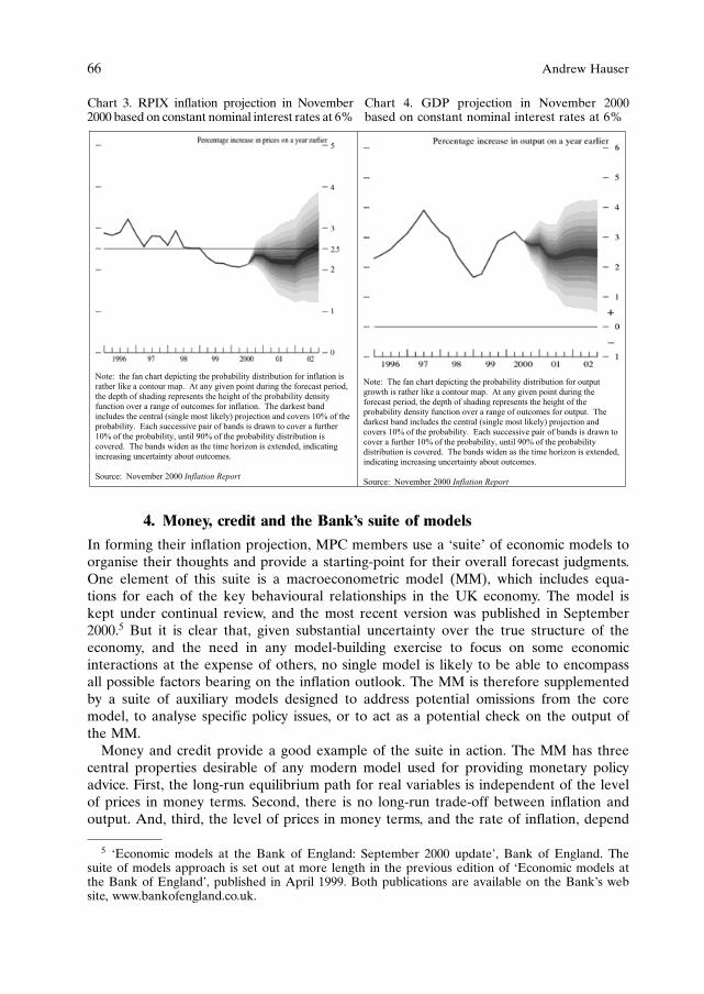
4. Money, credit and the Bank’s suite of models
In forming their inflation projection, MPC members use a ‘suite’ of economic models toorganise their thoughts and provide a starting-point for their overall forecast judgments.One element of this suite is a macroeconometric model (MM), which includes equa-tions for each of the key behavioural relationships in the UK economy. The model iskept under continual review, and the most recent version was published in September2000.5 But it is clear that, given substantial uncertainty over the true structure of theeconomy, and the need in any model-building exercise to focus on some economicinteractions at the expense of others, no single model is likely to be able to encompassall possible factors bearing on the inflation outlook. The MM is therefore supplementedby a suite of auxiliary models designed to address potential omissions from the coremodel, to analyse specific policy issues, or to act as a potential check on the output ofthe MM.Money and credit provide a good example of the suite in action. The MM has three
central properties desirable of any modern model used for providing monetary policyadvice. First, the long-run equilibrium path for real variables is independent of the levelof prices in money terms. Second, there is no long-run trade-off between inflation andoutput. And, third, the level of prices in money terms, and the rate of inflation, depend
66 Andrew Hauser
5 ‘Economic models at the Bank of England: September 2000 update’, Bank of England. Thesuite of models approach is set out at more length in the previous edition of ‘Economic models atthe Bank of England’, published in April 1999. Both publications are available on the Bank’s website, www.bankofengland.co.uk.
����� ��� �� ���� �� ���� ��� ���������� ����������� ��� ������� ��
������ ���� � ����� �� � �� �� ���� ��� ����� ��� ������� ������
��� �� �� �� ������ �� ������ ��� ������ �� ��� ���������� ������
����� ���� � ���� �� ������� ��� �������� ��� ������� ���
������ ��� ����� ������ ���� ������� ������� �� ����� � ! �� ���
����������� "�� �������� ��� �� ���� �� ���# �� ���� � �������
� ! �� ��� ����������� ���� $ ! �� ��� ���������� ����������� ��
������� ��� ���� #��� �� ��� ���� ����%� �� �&������ �������
������� �������� ����� ��������
'����� �������� ( ��������� ����
����� ��� �� ���� �� ���� ��� ���������� ����������� ��� ��� ��
���#�� �� ������ ���� � ����� �� � �� �� ���� ��� ����� ���
������� ������ ��� �� �� �� ������ �� ������ ��� ������ �� ���
���������� ������ ����� ���� � ���� �� ������� ��� ��� ��� ���
������� ��� ������ ��� ����� ������ ���� ������� ������� ��
����� � ! �� ��� ����������� "�� �������� ��� �� ���� �� ���# ��
���� � ������� � ! �� ��� ����������� ���� $ ! �� ��� ����������
����������� �� ������� ��� ���� #��� �� ��� ���� ����%� �� �&������
������� ������� �������� ����� ��������
'����� �������� ( ��������� ����
Chart 3. RPIX inflation projection in November2000 based on constant nominal interest rates at 6%
Chart 4. GDP projection in November 2000based on constant nominal interest rates at 6%

on monetary policy. In common with nearly all large-scale macroeconometric modelsused in other central banks and research institutions, however, whilst the MM containsa money demand equation, the potential active roles for money or credit in the trans-mission mechanism are less well-developed. If such models were the only tools used forgenerating inflation projections, these projections might miss important factors affectingthe outlook for inflation, at least under certain shocks or at certain points in the cycle.6
It is therefore important that the MPC has access to alternative models capable ofcapturing and quantifying any incremental information in money and credit, and actingas a cross-check on the output of the MM and other models in the suite. Extensiveresearch work at the Bank of England over the past few years has generated a rich setof empirical and theoretical models suitable for this purpose. Most of this material hasbeen published, and is available on the Bank’s web site.7 As part of the QMA, Bankstaff use these models to provide the MPC with an updated analysis of the potentialinformation in money and credit at an early stage in each forecast round.
5. The objectives of the Quarterly Monetary Assessment
Implicit in the suite of models approach is a recognition that views about the roleplayed by different variables, including (alternative definitions of) money and credit,may vary across academics, informed commentators and policy-makers. A central aimof the QMA is to reflect this range of views by offering policy-makers a menu of alter-native projections and simulations, depending on the extent to which monetary vari-ables are thought to be playing an active role in the transmission mechanism.Broadly speaking, monetary variables may be thought of as having three roles in
setting policy, and the content of the QMA reflects this. First, money and credit may beuseful indicators of developments elsewhere in the economy. Monetary statistics areavailable more rapidly than most other economic data, and are usually drawn from acomplete population, making them less vulnerable to sampling variation. So they mayassist policy-makers by providing an early, independent read on economic events in aworld of lagged and noisy data. Statistical evidence on the value of this information isgiven in Astley and Haldane (1995).Money and credit can be useful indicator variables even if they have no causal, or
amplifying, role in the transmission mechanism. If they do play such a role, however,they can also help policy-makers by providing incremental information on the transmis-sion of shocks through the system, at least at certain points in the cycle. This is likely tobe more of a medium-run exercise, and is one area where the models used in the QMAcan clearly complement the output of the macroeconometric model, and help to illumi-nate key issues in the preparation of the inflation projection. Encompassing this infor-mation reduces the probability of making policy mistakes.The third potential role for money and credit lies in signalling the long-run stance of
monetary policy – i.e. pressures likely to affect the medium to long-run determinationof inflation. On this view, money provides incremental information on the tightness orlooseness of policy over and above other measures, such as the short-term interest rate
Money and credit in an inflation-targeting regime 67
6 See, for example, Nelson (2000b) for a recent study of the possible incremental informationcontained in monetary variables.
7 A selection of references is given at the end of this paper; most are also available on theBank’s web site.
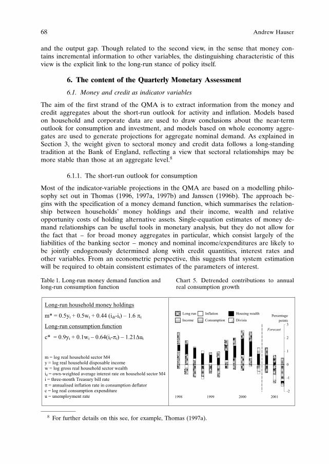
and the output gap. Though related to the second view, in the sense that money con-tains incremental information to other variables, the distinguishing characteristic of thisview is the explicit link to the long-run stance of policy itself.
6. The content of the Quarterly Monetary Assessment
6.1. Money and credit as indicator variables
The aim of the first strand of the QMA is to extract information from the money andcredit aggregates about the short-run outlook for activity and inflation. Models basedon household and corporate data are used to draw conclusions about the near-termoutlook for consumption and investment, and models based on whole economy aggre-gates are used to generate projections for aggregate nominal demand. As explained inSection 3, the weight given to sectoral money and credit data follows a long-standingtradition at the Bank of England, reflecting a view that sectoral relationships may bemore stable than those at an aggregate level.8
6.1.1. The short-run outlook for consumption
Most of the indicator-variable projections in the QMA are based on a modelling philo-sophy set out in Thomas (1996, 1997a, 1997b) and Janssen (1996b). The approach be-gins with the specification of a money demand function, which summarises the relation-ship between households’ money holdings and their income, wealth and relativeopportunity costs of holding alternative assets. Single-equation estimates of money de-mand relationships can be useful tools in monetary analysis, but they do not allow forthe fact that – for broad money aggregates in particular, which consist largely of theliabilities of the banking sector – money and nominal income/expenditures are likely tobe jointly endogenously determined along with credit quantities, interest rates andother variables. From an econometric perspective, this suggests that system estimationwill be required to obtain consistent estimates of the parameters of interest.
68 Andrew Hauser
�������� ������� ��� �������
� � ����� � ����� � ���� �������� � ��� ��
�������� ���� ����� �������
�� � ��!�� � ����� � ����������� � ��"����
� ��� �#� ������� ���� $�
� � ��� �#� ������� ����#%� ����
� � ��� ��� �#� ������� ���� �#���
�� � � � � � � � � � � � # ' � # � � � � � � � # � � � � � � � � � � � � � � $ �
� � ���� ���� (�#��� %��� �#�
� � #���#��� �� �#���� �#� �� ���� ����� � �#���
� � ��� �#� ���� ����� )�������
� � �� ���� �� �#��"
��
�
�
"
*
�!!+ �!!! "��� "���
,����#�
�����
��������
���� ��� -� �#���� .����� �#���
-��� /��� ����� 0�'��#
8 For further details on this see, for example, Thomas (1997a).
Table 1. Long-run money demand function and Chart 5. Detrended contributions to annuallong-run consumption function real consumption growth

The next stage of the Bank’s approach is therefore to specify a general vector autore-gression (VAR) in households’ money holdings, consumption, income, wealth, inflationand interest rates. From this system, two long-run relationships are identified, which –after imposing and testing a series of theory-consistent restrictions – are interpreted asa long-run consumption function and a money demand equation. Table 1 shows exam-ples of the type of equations achieved, taken from Thomas (1997a). Households’ reallong-run broad money holdings are increasing in both income and wealth, with a jointcoefficient of unity, increasing in the relative interest rate on deposits, and decreasing ininflation, proxying the relative return between real and financial assets. Real consump-tion is increasing in income and wealth – again with a joint unit coefficient – decreas-ing in a measure of the real interest rate, and decreasing in the change in unemploy-ment, a proxy for precautionary saving.If households’ actual money holdings were continuously demand-determined, if the esti-
mated money demand equation correctly captured the true structural relationship and if allof the right-hand side variables in the equation were measured without error in real time,money would contain no incremental information about the economy over and above thatcontained in those variables. In practice, however, none of these conditions is likely tohold. Even if money holdings were entirely demand-determined, data on money are avail-able earlier, and with less chance of error,9 than those on incomes, prices and wealth, so canprovide policy-makers with valuable indicator information. And the buffer-stock theory ofmoney demand suggests that agents may not always lie on their long-run demand function.If adjusting portfolios is costly, or yields are sluggish to adjust, households may be willingtemporarily to accept higher or lower money balances as an abode of purchasing power.Money demand equilibrium is then restored only gradually, as individual agents attempt toeliminate any excess holdings through purchases of goods and real and financial assets. Inthis scenario, money plays an incremental role in the transmission of shocks.These considerations suggest that there may be useful information in both money
growth, and in any gap between actual money holdings and the estimated long-rundemand. To capture both of these potential effects econometrically, the estimated long-run relationships are embedded in a first-difference VAR, and this system is then testeddown to give a parsimonious vector error correction mechanism (VECM) representa-tion. Consistent with the discussion above, residuals from the long-run money demandfunction are found to help explain the path of consumption. So the resulting systemexpresses consumption growth as a function of both monetary growth and ‘moneygaps’. For given assumptions about the exogenous variables, the model can therefore beused to generate ‘money-based’ projections for future consumption growth. The QMAinvolves a full description and analysis of these projections, together with a comparisonwith other non-money based profiles.An example of the type of analysis which can be presented to the MPC using this
class of model is given in Chart 5, which shows detrended contributions of the majordeterminants of real consumption growth from a version of the Janssen (1996b) house-hold Divisia10 model. For this particular projection, strong past growth in household
Money and credit in an inflation-targeting regime 69
9 Because they are drawn from a complete, or near-complete, population, so there should belittle or no sampling variation.
10 Divisia is a measure of money holdings that weights each component by a measure of itsliquidity and hence the likelihood that it will be used for consumer spending. The construction ofthe Bank’s Divisia indices is described in Fisher, Hudson and Pradhan (1992).

Divisia is predicted to lift consumption growth over the forecast period, but this effectis offset by other factors.Even within the class of monetary models, there is debate about which monetary aggre-
gate best captures the concept of money likely to be most closely associated with activity.So, as part of the QMA, forecasts are presented from both the household M4 and house-hold Divisia models, together with output from a model based on narrow money. Theseprojections have been helpful in highlighting influences on consumption which may havebeen missed by other forecasting approaches that omit an explicit role for money.
6.1.2. The short-run outlook for investment
A similar exercise is carried out for the corporate sector, using sectoral information onthe financial position of the corporate sector. The model used is based on Brigden andMizen (1999), and is functionally similar to the consumption model described above. Themain difference is that, in addition to equations for corporate money demand and invest-ment expenditure, the model also includes a long-run relationship describing firms’ bankborrowing. The rationale for this is that firms have greater capacity to manage their netliquidity position than households, so looking at only one side of their balance sheetscould give a particularly misleading picture. It also allows the model to capture elementsof any credit channel effects, which may affect certain firms (these are discussed in greaterdetail in Section 6.2). As with consumption, the model relates investment to both changeand disequilibrium terms in firms’ net liquidity position. The QMA shows projections forinvestment based on these relationships. And, as with consumption, the models also pro-vide a range of diagnostics, such as that given in Chart 6, which plots corporate borrowingand deposits relative to their estimated long-run levels. This type of analysis can help toenrich the analysis of particular forecast issues even where the QMA projections them-selves are not given a central role in the MPC’s own assessment.Recent years have seen significant changes in the structure of corporate finance in
the UK. A stronger government fiscal position and lower inflation, together with in-creased internationalisation and innovation in capital markets, have led firms progres-sively to shift more of their liabilities from bank to market-based finance (see Chart 7).
70 Andrew Hauser
���
���
���
��
�
�
��
��
��
���� ���� ���� ��� ���� ����
�� ���
���������
��������
�
�
��
��
��
��
���� ��� ��� ���� ���� ����
�� ���
Chart 6. Corporate money and credit: deviationfrom estimated equilibrium levels
Chart 7. Bank borrowing as a proportion of thetotal financial liabilities of the corporate sector

As a result, some of the traditional relationships between bank deposits, credit andinvestment have become less reliable over time. The links between firms’ overall finan-cial position, activity and inflation remain a key focus of policy-makers’ concerns, how-ever, and this has suggested a number of new avenues for research. Recent Bank workhas, for instance, included the development of a calibrated corporate ‘financial accelera-tor’ model for the UK, along the lines of that proposed by Bernanke, Gertler andGilchrist.11 This class of model links firms’ spending behaviour to their overall financialposition via an external finance premium, and offers a potentially rich range of insightsinto the role of credit in the transmission mechanism, the effects of financial innova-tion, and the impact of bubbles and other asset price phenomena.
6.1.3. The short-run outlook for aggregate nominal activity
The final element of the indicator-variable component of the QMA uses VECMs basedon whole-economy money aggregates to derive short-run forecasts for nominal GDP,inflation and real activity. Again, a range of projections are presented from modelsbased on alternative monetary aggregates: narrow money (M0), retail money (M2) andbroad money (M4). Those who believe that base money contains most informationabout the stance of monetary policy, and therefore inflationary pressures, may placegreatest weight on the output of the M0 model. And those who place more faith inbroader aggregates may take greater notice of the M2 and M4 model projections.The reason for producing models based on both M2 and M4 relates mainly to the
behaviour of non-bank financial firms, or ‘OFCs’, the money holdings of which arecaptured in M4, but have little impact on M2. Recent years have seen sharp growth inOFC balance sheets, associated with the structural changes to the corporate sector dis-cussed above, the growth in asset prices, the increased use of securitisations of retailportfolios, and so on. This growth has also been associated with sharp fluctuations inOFCs’ money holdings, and therefore in M4 (see Chart 8). Some commentators believethat the money holdings of at least part of the OFC sector may have a causal impacton inflation via their effects on asset prices. Others prefer to see OFCs’ money as pri-marily reflecting volatile financial activity, or the precise way in which financing ar-rangements are constructed, with little implication for the prices of goods and ser-vices.12 In the absence of conclusive evidence it is important that policy-makers haveaccess to projections consistent with either interpretation. The QMA therefore presentsforecasts from both M2 and M4 models.One simple way of deciding on which model to rely most is to weight the projections
of each model according to their past performance. The QMA therefore also provides asummary set of forecasts formed by weighting together the outputs of the M0, M2 andM4 models. To the extent that the explanatory power of each model may vary accord-ing to the nature of the shocks hitting the economy, however, such a fixed weightingscheme may be less appropriate. The summary diagnostic is therefore shown in addi-tion to, and not instead of, the output of the individual models.
Money and credit in an inflation-targeting regime 71
11 See, for example, ‘The financial accelerator in a quantitative business cycle framework’ inTaylor, J.B. and Woodford, M. (eds), Handbook of Macroeconomics, Amsterdam: New Holland.
12 These issues have been regularly discussed in the Bank’s Inflation Report. See, for instance,the box on pages 6–7 of the May 1998 Report.

6.2. Money, credit and the transmission mechanism
The second component of the QMA covers money, credit and the transmission me-chanism. Much of this involves a careful assessment of prevailing credit conditions. Akey insight from the recent ‘credit channel’ literature13 is that – contrary to the pre-dictions of simple neoclassical models – credit may play a separate role in the propa-gation of economic shocks. This issue is likely to be most acute at times of potentialfinancial instability, such as the events related to Russia and LTCM in 1998, whenpolicy-makers spent considerable time assessing the financial health of the UK finan-cial and private sectors.14 But it is not necessarily limited to such periods. As therecent financial accelerator literature stresses, if the effective cost of capital dependsnot just on observed rates but also on agents’ financial positions, credit conditionscould also contain incremental information relevant to an assessment of the true cycli-cal position of the economy.At present, much of the QMA assessment in this area is based on careful data analy-
sis, backed by a substantial pack of charts and tables summarising the latest develop-ments in credit conditions. The analysis includes a review of households and firms’financial positions – including an assessment of gearing levels – a review of non-pricecredit effects and an appraisal of the private sector’s borrowing capacity. A simple ex-ample of the type of data on which this analysis is based is given in Chart 9, whichcompares households’ debt/wealth and debt/income ratios, two alternative measures ofhousehold gearing.Increasingly, however, this analysis is also being informed by the type of more formal
theoretical and empirical work discussed elsewhere in this paper. As mentioned above,the Bank has developed a calibrated financial accelerator model of the UK corporate
72 Andrew Hauser
�
�
�
�
�
��
��
��
�� �� �� �� ��
��� �� ������ �� � �� ���
�� ��
��
13 A summary of key aspects of this literature is given in ‘Inside the black box: the credit channelof monetary policy transmission’ by Bernanke, B. and Gertler, M., Journal of Economic Perspec-tives, 1995, Vol. 9, pages 27–48.
14 See, for instance, section 1 of the November 1998 Inflation Report.
Chart 8. Monetary growth

sector. Work is currently under way on a similar model for the household sector. And itis hoped that in the future these theoretical models will be supplemented by moredetailed econometric studies based on micro data sets. An attractive aspect of the cali-brated theoretical models is that they not only provide a quantitative link betweenmeasures of financial health and expenditures, they also allow staff to perform a widevariety of scenario analyses based on alternative hypotheses about possible futureshocks or changes to the structure of the economy, such as financial innovation. Anexample of this type of analysis is given in Chart 10, which shows how the response ofinvestment in the model to a monetary policy shock varies under alternative assump-tions about gearing levels. Because of its relative simplicity, the model does not captureevery aspect of the data – such as the speed of adjustment in response to shocks –particularly well. But it can, for example, be used to provide an estimate of the incre-mental effect of higher gearing on the level of investment under alternative scenarios.
6.3. Measures of the longer-term monetary stance
The final element of the QMA is based on the idea that data on money and credit maycontain information relevant to the assessment of the monetary stance – and thereforelonger-run inflationary pressures. As a simple cross-check, the MPC is presented withthe output from some simple monetary policy rules, including a McCallum rule15 esti-mated for the United Kingdom and a Taylor rule.16 It also includes a rule based on anempirical implementation of the Brainard17 result, which suggests that policy-makerswho are uncertain about key parameters in the economy may in certain circumstances
Money and credit in an inflation-targeting regime 73
15 McCallum’s original rule for the United States is given in ‘Robustness properties of a rule formonetary policy,’ Carnegie-Rochester Conference Series on Public Policy, Volume 29, 1988, pages53–84.
16 Taylor’s original rule for the United States is given in ‘Discretion versus policy rules in prac-tice’, Carnegie-Rochester Conference Series on Public Policy, Volume 39, 1993, pages 195–214.
17 See ‘Uncertainty and the effectiveness of policy’, Brainard, W., American Economic Review,Volume 57, 1967, pages 2–19.
��
��
��
��
��
��
��
���� ���� ���� ���� ���� ���� ����
�
�
��
��
�
�
�� ����� ���
���� ���� � ��� ������
���������� � ����
���� ���� � �� � �
���!������� � ����
��
��
�"
��
�
��
�
� � � " � � � � � �� �� �
�� ����!� ��#������ ��� �����$ ����� ��#��
%&������ ����� ��� �
'�� ��(����� !�����!
)�!� ��(����� !�����!
Chart 9. Household sector gearing ratios Chart 10. Response of investment to a 100basis points monetary policy shock
behave more conservatively, and draws on published work by Martin and Salmon(1999). Bank staff are developing a range of other measures of the monetary stance,which may be used in future QMAs.In addition to these measures, the MPC is provided with an analysis based on a
monetary structural VAR (or SVAR) of the UK economy developed by Dhar, Pain andThomas (2000). An important lesson drawn from experience with earlier models wasthat, in general, there is no single deterministic link between money, activity and infla-tion. In practice, all three are endogenous to some degree, so the precise relationshipswill depend on the fundamental shocks driving the economy at any point in time. Pol-icy-makers should therefore beware of drawing firm inferences about future inflation-ary pressures solely on the basis of simple monetary statistics. Before drawing policyconclusions, a view must be taken on the likely structural shocks driving the economy.SVARs represent one way of attempting to identify these shocks.The model used in the QMA is estimated as follows. Starting from an eight-variable
levels VAR in real money, incomes, inflation and a vector of asset prices, four long-runrelationships are identified, including a money demand equation, a term structure rela-tionship, and an asset pricing function. Theory-based restrictions are then used to iden-tify four permanent and four temporary shocks. These include both temporary and per-manent monetary policy shocks, and two types of velocity shock, one reflecting changesin the provision of credit by the banking system, and one reflecting changes in liquiditypreference.In the model, different shocks have different implications for the cross-correlation
patterns of money, activity and prices. This has long been understood in a relativelyinformal way from the monetary assessment side. But the formalisation and quantifica-tion of this idea represents a key advance from this research. The model also providesBank staff with a highly flexible tool for use in longer-term policy analysis and advice.
7. The MPC’s inflation projection, the suite of models and the QMA
The inflation projection published in the quarterly Inflation Report is drawn up by, andowned by, the MPC. In producing its forecast, assisted by Bank staff, the Committee isable to draw on the analysis prepared in the QMA, other parts of the suite of models,or any other sources. In principle, the MPC might use the QMA output in severaldifferent ways. First, the indicator-variable projections might be used to help set theshort-term constraints for the MPC’s own central projection, improving the data set forthe very near-term outlook. Second, the material on money and credit in the transmis-sion mechanism might be used to adjust the output of simpler equations on the MM orelsewhere where it was thought that the money or credit data contained incrementalinformation. Third, the longer-run projections and measures of monetary stance providea potential cross-check on the provisional outputs of the forecast. And, fourth, any orall of the QMA material could help the MPC to assess the risks around possible centralprojections, reflected in the inflation and GDP fan charts, or the table in Section 6 ofthe Inflation Report, which records alternative views about the inflation and activityoutlook.By providing a menu of alternative projections, the QMA recognises that different
policy-makers may have different interpretations of, or put different weights on, devel-opments in the money and credit data. Some of the models described here may also be
74 Andrew Hauser

thought to have more relevance at some points in the cycle, or in certain market condi-tions, than others. There is therefore no mechanical link between the material provided,and the MPC’s final projections for GDP and inflation. Nevertheless, it is importantthat Committee members are made aware of, and are able to draw on, the best possi-ble technical representations of these alternative paradigms if they are to minimise therisks of making policy mistakes.
8. Conclusions and challenges for the future
Whilst understanding of the role of money and credit has developed considerably overthe past twenty years, much remains to be done. Reflecting this, Bank staff are highlyactive in monetary research and analysis, and the results of this work are regularly usedto update and extend the contents of the QMA. There are many potential avenues forinvestigation, but three broad themes stand out.First, the difficulty of predicting trend velocity remains a key challenge, both for
policy analysis and for technical modelling. After a period of relative stability in thefirst half of the 1990s, both narrow and broad money velocity has fallen sharply in theUK. Lower inflation and nominal interest rates may be able to explain part of thisshift, but by no means all. Understanding the reasons for this shift, and predicting whenand where it may end, is a key priority.Second, and closely related, monetary analysts need to remain abreast of the devel-
oping role of money and credit in a world of constant structural change. The financialstructure in the UK and elsewhere continues to evolve rapidly. Recent years have seena substantial shift of corporate finance away from bank, and towards non-bank, sources(a trend accompanied by a sharply increased role for non-bank financial intermedi-aries). There has been extensive innovation in retail markets. And the move to a lower-inflation environment has had a series of effects on the demand for money and credit.These and other developments create new challenges for our understanding of the roleof financial quantities variables.Third, experience at the Bank of England in recent years has underlined the impor-
tance of understanding the nature of the economic shocks affecting the money andcredit aggregates. Whilst central banks have accrued enormous experience in shorter-term analysis of the monetary data, more work needs to be done in using these lessonsto shape and inform our more formal technical and empirical models. And there areimportant lessons to be learned from real-side research and analysis, much of which isgrappling with similar issues.This is a challenging agenda. But it emphasises the importance of continuing to push
forward our understanding of monetary developments. The Bank of England hopes toplay a full part in this debate.
References: selected Bank of England research
Astley, M. and Haldane, A.G. (1995), ‘Money as an indicator’, Bank of England,Working Paper 35.Astley, M. and Haldane, A.G. (1997), ‘Money as an indicator’, Bank of England, Quarterly Bulle-
tin, Vol 37, pages 174–180.Batini, N., Hall, S., Salmon, C. and Yates, A. (1999), ‘Uncertainty and simple monetary policy rules
– an illustration for the United Kingdom’, Bank of England, Working Paper 96.Brigden, A. and Mizen, P. (1999), ‘Money, credit and investment in the UK corporate sector’,Bank of England, Working Paper 100.
Money and credit in an inflation-targeting regime 75

Brigden, A., Chrystal, A. and Mizen, P. (2000), ‘Money, lending and spending: a study of the UKnon-financial corporate sector and households’, Bank of England, Quarterly Bulletin, Vol 40,pages 159–167.
Chrystal, A. and Mizen, P. (1999), ‘Money, credit and investment in the UK corporate sector’,Bank of England, Working Paper 100.
Dhar, S.K. and Millard, S.P. (2000a), ‘A limited participation model of the monetary transmissionmechanism in the United Kingdom’, Bank of England, Working Paper 117.
Dhar, S.K. and Millard, S.P. (2000b), ‘How well does a limited participation model of the monetarytransmission mechanism match UK data?’, Bank of England, Working Paper 118.
Dhar, S.K., Pain, D. and Thomas, R. (2000), ‘A small structural empirical model of the UK mone-tary transmission mechanism’, Bank of England, Working Paper 113.
Fisher, P.G., Hudson, S. and Pradhan, M. (1992), ‘Divisia indices for money: an appraisal of theoryand practice’, Bank of England Working Paper 9.
Goodhart, C.A.E. and Crockett, A. (1970), ‘The importance of money’, Bank of England, Quar-terly Bulletin, Vol 10, pages 159–198.
Haldane, A.G., McCallum, B.T. and Salmon, C. (1996), ‘Base money rules in the United Kingdom’,Bank of England, Working Paper 45.
Janssen, N. (1996a), ‘Can we explain the shift in M0 velocity? Some time-series and cross-sectionevidence’, Bank of England, Quarterly Bulletin, Vol 36, pages 39–50.
Janssen, N. (1996b), ‘The demand for Divisia money by the personal sector and by industrial andcommercial companies’, Bank of England, Quarterly Bulletin, Vol 36, pages 405–411.
Janssen, N. (1998), ‘The demand for M0 in the United Kingdom reconsidered: some specificationissues’, Bank of England, Working Paper 83.
Martin, B. and Salmon, C. (1999), ‘Should uncertain monetary policy-makers do less?’, Bank ofEngland Working Paper 99.
Nelson, E. (2000a), ‘UK monetary policy 1972–97: a guide using Taylor rules’, Bank of England,Working Paper 120.
Nelson, E. (2000b), ‘Direct effects of base money on aggregate demand: theory and evidence’,Bank of England, Working Paper 122.
Price, L.D.D. (1972), ‘The demand for money in the United Kingdom: a further investigation’,Bank of England, Quarterly Bulletin, pages 43–55.
Thomas, R. (1996), ‘Understanding broad money’, Bank of England, Quarterly Bulletin, Vol 36,pages 163–179.
Thomas, R. (1997a), ‘The demand for M4: a sectoral analysis – Part 1 – The personal sector’,Bank of England, Working Paper 61.
Thomas, R. (1997b), ‘The demand for M4: a sectoral analysis – Part 2 – The corporate sector’,Bank of England, Working Paper 62.
76 Andrew Hauser

1. Introduction
The principle that inflation and deflation are fundamentally monetary phenomena hasbeen one of the best understood and empirically well founded notions in monetaryeconomics. Over history, whenever central banks have allowed money growth to sys-tematically surpass the natural growth of the economy, sooner or later inflation inevita-bly followed. Likewise, serious deflationary episodes have invariably been associatedwith sustained shortfalls in money growth.
Recognition of this fundamental principle over the years has led many central banksto place special emphasis on reigning in money growth in a continuing effort to pursueand maintain price stability over time. And consequently, monitoring the growth rate ofmoney has long been part of the standard monetary practitioner’s toolkit.
In the United States, it is by now well understood that the two episodes most com-monly seen as major monetary policy failures since the founding of the Federal Re-serve, namely the Great Depression of the 1930s and the Great Inflation of the 1970s,were episodes where policymakers failed to properly monitor and heed the warningspresent in the behavior of money. In large part because of these experiences, the Feder-al Reserve has regularly monitored the growth of money since the late 1970s.
However, the behavior of monetary aggregates may not always serve as a particu-larly reliable guide to inflation. Over shorter horizons, in particular, cyclical develop-ments and transitory changes in the velocity of money present non-trivial complications.Simple measures of money growth may not always reliably foreshadow subsequentmovements in inflation. From this perspective, the benefits of close monitoring of thebehavior of monetary aggregates as indicators of inflation over shorter horizons maynot always appear very large.
The process of constructing monetary aggregates is inherently an empirical enter-prise, fraught with the difficulties of any such enterprise. Over longer horizons, financial
Money and inflation: the role of information regardingthe determinants of M2 behavior
Athanasios Orphanides and Richard D. Porter*
Board of Governors of the Federal Reserve System
* Helpful comments by our discussant, Maria Valderrama and seminar participants at the ECBSeminar on “Monetary Analysis: Tools and Applications” are greatly appreciated. The opinionsexpressed are those of the authors and do not necessarily reflect the views of the Board of Gover-nors of the Federal Reserve System or its staff. Correspondence: Orphanides: Division of Mo-netary Affairs, Board of Governors of the Federal Reserve System, Washington, D.C. 20551,tel.: (202) 452-2654, email: [email protected]. Porter: Division of Monetary Affairs, Boardof Governors of the Federal Reserve System, Washington, D.C. 20551, tel.: (202) 452-2497,email: [email protected].

innovation and secular changes in the economy imply that the meaning and usage ofmoney may evolve over time in ways that may require reevaluation of existing empiri-cal concepts and measurement methods regarding the aggregates. The creation of anew financial instrument, for instance, typically requires a judgment regarding its place-ment within existing definitions of the monetary aggregates and could lead to long-runchanges in the velocity of circulation of existing measures. Such innovations often re-quire time and internal debate before the appropriate treatment can be determined.They also highlight that, as a practical matter, there is not, indeed there cannot be, aunique satisfactory empirical definition of money. And this difficulty is one reason whymultiple measures are typically defined and monitored.
Because of these difficulties, the empirical usefulness of monetary aggregates as indi-cators of inflation over various horizons depends on the ability of central banks todistinguish movements in the aggregates that reflect underlying inflationary develop-ments from those that arise as a result of other factors. This ability may be quite diffi-cult to quantify in practice. For example, despite their general usefulness, simple statisti-cal techniques mechanically applied to aggregate data cannot capture informationregarding special factors influencing specific monetary aggregates at any given time.Such techniques may also fail to detect important structural shifts in statistical relation-ships that could be explained – sometimes even predicted – if additional informationwere brought to bear. Indeed it is precisely for this reason that judgment plays animportant role in interpreting monetary aggregates in practice.
Surely, interpreting monetary aggregates may be a highly uncertain task, especiallyduring periods when structural change is potentially occurring. However, central banksby the very nature of their operations, such as the close contact with financial institu-tions and markets, and the continuous monitoring of banking institutions, including thesystematic collection of detailed information on bank balance sheets, are in a uniqueposition to accumulate and interpret information regarding monetary aggregates. Fail-ing to account for this central bank capability may easily obscure the usefulness ofmonetary aggregates. But neither the uncertainty involved in the process, nor the diffi-culty of quantifying the usefulness of monetary aggregates imply that the emphasisplaced by central banks on monitoring monetary aggregates is misplaced.
In this paper, we examine the relationship between the behavior of M2 and inflationin the United States over the past forty years and attempt to draw some lessons regard-ing the usefulness of employing this aggregate for guidance regarding inflation. In parti-cular, we investigate the role of changes in equilibrium velocity in understanding therelationship between M2 and inflation and also examine the role of special factors inassessing the underlying strength of money growth. Examining the behavior of M2 inthis regard is particularly helpful for two reasons. First, because the behavior of M2 hasbeen monitored relatively closely by the Federal Reserve during the past two decadesand was one of the aggregates emphasized by the Federal Reserve for communicatingmonetary policy during this period. Second, because a number of factors including amajor wave of restructuring in the banking sector and financial innovation dramaticallychanged the velocity of the aggregate over a period of several years during the early1990s. These developments created considerable difficulties and uncertainty in interpret-ing the behavior of the aggregate during that period.
We use the experience of M2 during the 1990s as an example to illustrate how failingto account for changes in equilibrium velocity could have obscured the usefulness of
78 Athanasios Orphanides and Richard D. Porter

M2 in providing information regarding inflation. In addition, using examples from the1990s, we discuss the relevance of taking into account special factors in evaluating themovement in this aggregate.
2. Velocity and the equation of exchange
The equation of exchange defines the velocity of money and serves as the cornerstonefor virtually any examination of the relationship between money and inflation. Let Mdenote the stock of money in circulation, Q real output and P its price. The equation ofexchange defines the velocity of money, V, such that
MV ¼ PQ : ð1Þ
If the velocity of money were nearly constant over time or nearly perfectly predictable,this relationship would present a direct and immediate link between money and nom-inal income so that, controlling for cyclical fluctuations in real output, the price leveland inflation could be read simply by observing money. In practice, the velocity ofmoney may vary considerably over time and, as a result, understanding its movementsbecomes essential in assessing the inflationary implications of particular patterns ofmoney growth. The solid line in Figure 1 plots the velocity of M2 in the United Statesfrom 1960 to 2000.1 The plot confirms that there has been significant variation in thismeasure of velocity.
It is useful to be aware of and distinguish between two potential sources of this varia-tion, namely changes in the underlying trend of velocity such as due to the continuingimprovement of financial services and financial innovation, and cyclical changes asso-ciated with short-run deviations of velocity from its underlying long-run trend. Twoalternative estimates of the underlying trend are plotted in Figure 1. The first representsa linear trend fit through the logarithm of velocity using data from 1960 to 1989 only(the dotted line). As can be seen, since perhaps 1992, actual velocity has deviated sys-tematically from this underlying trend in a way that suggests a possibly gradual upwardshift in equilibrium velocity. Thus, based on the history of velocity during the 1990s, thelinear trend estimated and evident over the earlier sample does not appear as an ade-quate representation of the underlying trend over the full period. The plot also showsan alternative estimate, which is represented by the smooth trend plotted with a dashedline. This measure captures a gradual increase in velocity during the early 1990s, sug-gesting a significant upward shift by the mid 1990s, which lies above the earlier estab-lished trend in velocity.
Although this figure indicates that the underlying trend in velocity veered upwards, itdoes not make clear how one could determine with any accuracy when exactly thisupturn may have occurred and whether the change was gradual or not. Equally impor-tantly, it does not offer guidance as to how one could have detected this shift early inthe 1990s based on this one series alone. Compare, for instance, the increase in velocityfrom 1976 to 1980 and the increase from 1989 to 1993. The two appear about as steepand virtually equally dramatic. In retrospect, the late 1970s shift appears to have beenalmost certainly transitory in nature while the early 1990s shift appears to be a perma-nent feature of the data. Such a distinction, however, cannot be reliably made without
Money and inflation 79
1 This chart utilizes quarterly data available as of November 2000.

additional information. Though making such a distinction may appear problematic atfirst, it can actually be quite simple and straightforward once additional information isbrought to bear.
Traditional theories of the demand for money posit that velocity fluctuates from itsunderlying trend with the opportunity cost of holding money, OC. Letting gOCOC denotedeviations of the opportunity cost of money from its average norm, a simple way tocapture this relationship is as follows:
log ðVtÞ � log ðV*tÞ ¼ a1gOCOC þ ut : ð2Þ
If the variation in the opportunity cost accounts for a large fraction of the variation ofvelocity from its underlying trend, V*, using this relationship would make detection ofchanges in the underlying trend much easier. Figure 2 plots M2 velocity against theopportunity cost of M2 and confirms that such costs do explain a large fraction of thecyclical movements in velocity. We construct the opportunity cost of M2 as the differ-ence between the yield on the 3-month Treasury bill and the average rate paid on M2balances. As shown, while a small linear trend may have indeed been an adequate charac-terization of the underlying trend in V2, starting as early as 1990 a divergence in thebehavior of velocity relative to the behavior of its opportunity cost could be observed. By1991 the evidence for a significant structural change was becoming overwhelming.
The following regression combines the systematic money demand relation posited inequation (1) with a smooth underlying trend for velocity:
log ðVtÞ ¼ a0 þ a1gOCOC þ a2TIMEt þ a3St þ ut ; ð3Þ
80 Athanasios Orphanides and Richard D. Porter
Figure 1. M2 Velocity and Underlying Trends
Notes: The linear trend is estimated by regressing the logarithm of M2 velocity on a time trendfrom 1960 to 1989. The smooth trend extends the sample to 1999 and is estimated as explained inthe text.

where
St ¼1
1 þ e�xðt�tÞ : ð4Þ
The estimation defines implicitly the trend underlying equilibrium velocity as:
log ðV*tÞ ¼ a0 þ a1TIMEt þ a3St : ð5Þ
This specification nests the linear trend specification, a3 ¼ 0, as well specifications al-lowing for a one time shift in the equilibrium velocity as could be captured by a dum-my variable. To see this point, observe that for very large values of x, St essentiallycollapses to a step function that equals zero when t < t and equals one when t > t. Inthis case, the estimate of t offers the best estimated location of the structural breakrepresented by introducing a dummy variable into the demand function.2
Estimation of equation (3) with non-linear least squares yielded the estimatedsmooth trend for equilibrium velocity shown in Figure 1. The estimated midpoint of thetransition (determined by t) is 1992Q3. The data suggest that this shift did not takeplace overnight with the speed of the transition (determined by x) indicating that aboutone quarter of the adjustment had taken place by 1991Q2 and about three quarters by1993Q4.3
Money and inflation 81
Figure 2. Velocity and Opportunity Cost
2 This specification, of course, should be seen as one of several possible approximations for detect-ing and capturing the 1990s shift in M2 velocity. For instance, Carlson, Craig and Schwartz (2000),Carlson, Hoffman, Keen and Rasche (2000) and Sephton (2000) examine alternative treatments.
3 While our argument does not depend on what caused the shift in velocity in the early 1990s,our assessment is that the inclusion of the smooth velocity shift term may be an appropriate model-ing strategy, at least given our understanding of the forces at work. One of the most importantforces was the thrift and banking crisis. The resulting closure of institutions greatly disrupted de-

Figure 3 plots the resulting velocity gap, that is the difference between actual velo-city, V, and its underlying equilibrium trend, V*, against the opportunity cost of M2balances. As can be seen, once the gradual increase in equilibrium velocity is accountedfor, the variation in the velocity gap can in large part be accounted for by the variation ofthe opportunity cost of M2 balances both before the 1990s as well as during the 1990s.
An important question is the extent to which the dramatic shift in equilibrium velo-city reflected in the smooth estimate in Figure 1 was detected in real-time or couldhave been detected during the transition e.g. around 1992–1993. In an earlier study,Orphanides and Porter (2000), we demonstrated how the shift could have been pickedup in real-time, as it was in actuality. Indeed, the shift in equilibrium velocity was
82 Athanasios Orphanides and Richard D. Porter
Figure 3. Velocity Gap and Opportunity Cost
posit relationships, sometimes repeatedly, particularly in the case of brokered CD accounts at high-flying thrifts. This crisis also altered the legislative and regulatory landscape in significant ways. Itlowered the safety net on deposits. It made banks and not the government bear more of the bur-den for mistakes, and it led to a significant tightening up on lending standards. At the same time,as depositors were feeling more uncertain about their banking relationships, stock and bond mu-tual funds were successfully gearing up to market an array of attractive fund products in an envir-onment of a very steep yield curve, which apparently induced many households to reach for yield.The forces, which produced the shift, were thus numerous and undoubtedly interacted with oneanother. But, the most important thing to note is that none of the forces were primarily cyclical innature but were secular, suggesting that a smooth time trend may be an adequate way to representthem. Thus, their existence does not in itself have to necessarily disrupt the cyclical part of therelationship embedded in the opportunity cost term. See Feinman and Porter (1992) for a contem-poraneous attempt to understand the resulting weakness in M2, Orphanides, Small and Reid(1994) for an analysis of the resulting substitution of M2 balances with stock and bond mutualfunds and Lown, Peristiani, and Robinson (1999) for a more recent perspective on the episode.
Notes: The velocity gap is defined as the logarithmic difference between M2 velocity and the esti-mated equilibrium velocity corresponding to the smooth trend in Figure 1.

detected as early as 1991, although at the time it was obviously quite unclear how largeand how long lasting the shift in equilibrium velocity would be. And, as we illustratedin our earlier study, simple statistical techniques, which recursively estimated new levelsof V* by incorporating the information regarding the divergence of V2 from its earlierrelationship with the opportunity cost of M2, also captured this change, though withsomewhat less precision and after some lag. Figure 4 compares the velocity gap ob-tained from one such recursive real-time estimate of V* with the gaps based on thelinear and smooth trend estimates shown in Figure 2. The recursive estimate showncorresponds to Estimate B in our earlier study. It allows for a time trend in velocityand one discrete shift captured by a dummy variable. Of the alternatives discussed inour earlier study, this specification is the one most closely related to our simple ex postcharacterization of equilibrium velocity shown in equation (5).4 As is evident, incorrectreliance on a constant trend would have resulted in estimated velocity gaps that de-viated substantially from the more accurate representation offered by the smooth trendestimate. On the other hand, the recursive estimates are much closer to the gaps basedon the smooth trend and in that sense much less misleading.
The necessity of accounting for the movements of velocity for interpreting the beha-vior of money and its relationship to inflation is well understood. As we illustrate inthis section, ignoring readily available information regarding changes in the underlyingtrend of velocity can lead, at least temporarily, to misleading interpretations of velocity.
Money and inflation 83
Figure 4. Alternative Velocity Gaps
4 The V� estimates used here were updated using current data to extend the sample coverageand maintain consistency with the other series employed in this study.
Notes: Each velocity gap is defined as the logarithmic difference between M2 velocity and an esti-mate of equilibrium velocity. The gaps based on the linear and smooth trends are based on thecorresponding estimates shown in figure 1. The real-time gap is based on the recursive estimatesdescribed in the text.

In the next two sections we investigate how accounting for this information regardingthe changes in the equilibrium velocity of M2 during the first part of the 1990s couldinfluence inference regarding the usefulness of M2 as both an anchor and indicator ofinflation.
3. Money growth and inflation
Rewriting the equation of exchange in growth terms, approximated by logarithmic dif-ferences, allows restating this identity in terms of money growth and inflation. In thissection, we use this well-known relationship to illustrate in a simple manner the signifi-cance of properly accounting for changes in equilibrium velocity in assessing the useful-ness of money growth as an anchor for inflation.
For notational convenience, we use lowercase letters to denote logarithms, and adoptthe standard notation p ¼ Dp for inflation and m ¼ Dm for money growth. Writing theequation of exchange in logarithmic form, mþ v ¼ pþ q, and taking differences gives:
m þ Dv ¼ p þ Dq : ð6Þ
As with the equation of exchange, this relationship is an identity and holds for anyhorizon over which growth rates are computed. To allow for a more convenient inter-pretation, it is useful to decompose the growth of output and growth of velocity intotheir long-run equilibrium components and cyclical components. Defining Q* to denotethe natural level of output (potential output), the cyclical component of output growthcan be captured by the growth rate gap, ðDq� Dq*Þ. Likewise, the cyclical componentof velocity growth can be captured by the velocity growth gap, ðDv� Dv*Þ. By defini-tion, both of these gaps tend towards zero as the growth rates are computed over longerhorizons.
Equation (6) can be restated in terms of the cyclical and long-run components ofoutput and velocity growth as follows:
m þ Dv* þ ðDv� Dv*Þ ¼ p þ Dq* þ ðDq� Dq*Þ : ð7Þ
Rearranging terms to express this relationship in terms of inflation yields:
p ¼ m � Dq* þ Dv* � ðDq� Dq*Þ þ ðDv� Dv*Þ: ð8Þ
This equation suggests a convenient decomposition of inflation into a cyclical compo-nent and a component determined by money growth adjusted both for the naturalgrowth of output and changes in equilibrium velocity. Let m* reflect this adjustedmoney growth:
m* � m � Dq* þ Dv*: ð9Þ
Collecting the two cyclical terms:
h ¼ �ðDq� Dq*Þ þ ðDv* � DvÞ
and rewriting equation (8) yields:
p ¼ m* þ h : ð10Þ
84 Athanasios Orphanides and Richard D. Porter

As this equation makes obvious, apart from cyclical effects that tend towards zeroover medium- and long-term horizons, inflation should track adjusted money growthclosely. Equation (10), of course, is simply a restatement of a relationship that is bothfundamental and well understood. If the central bank’s long-run objective is toachieve and maintain inflation at a low and stable level, p*, then this relationshipindicates that the central bank must ensure that money growth is set such thatp* ¼ m* over time.
The relationship embedded in equation (10) has served as the basis for determiningreference and monitoring values for the growth of monetary aggregates for a long time.Milton Friedman’s famous prescription during the late 1960s and early 1970s that mone-tary policy in the United States should aim to keep the growth rate of M2 stable atfour percent serves as an example. His prescription was based on the observation thatequilibrium M2 velocity appeared to be close to a constant and the consensus view atthe time that the natural growth rate of output was four percent. The prescription sug-gested that abstracting from cyclical effects, stable M2 growth at a four percent levelwould achieve near price stability. Another example is the monetary frameworkadopted by the Bundesbank from the mid 1970s until the 1990s.
Although the relationship between inflation and money growth in equation (10) fol-lows from an identity and should be beyond dispute, it is not always sufficiently appre-ciated. There are at least two reasons for this confusion. First, over short horizons, thisrelationship is in large part overshadowed by cyclical factors. Second, without the prop-er adjustment for changes in Q* and V*, money growth and inflation may not appearto track each other even over medium-run horizons. We illustrate each of these difficul-ties in turn.
In Figure 5 we plot inflation over four quarters against the growth rate of moneyover the same horizon adjusted for the natural growth rate of the economy.5 (Asmentioned earlier, this adjustment alone suffices if V* is believed stable or has only asmall constant trend. We examine shifts in V* below.) The figure covers the 1965–2000 period, which includes the Great Inflation of the late 1960s and 1970s and thesubsequent disinflation. Although the long inflation/disinflation cycle is evident in theinflation series, the growth rate of money exhibits such a high degree of volatility,especially during the first half of the sample, that the strong correlation over themedium run between the trend in inflation and that of money growth is rather diffi-cult to detect in this figure. Concentrating on the period from 1965 to 1979 it is alsoclear from the figure that if the relationship between inflation and money growthwere examined after first detrending the series, the data would suggest a strong nega-tive correlation between inflation and money growth instead of a positive one. Theobvious pitfall here, of course, comes from the fact that the most useful piece ofinformation provided by money growth regards lower frequency movements in infla-tion so that any detrending of the series removes a crucial piece of information fromthe analysis. Although it is not uncommon in practice, detrending of inflation may bea seriously flawed procedure in disentangling the relationship between monetary ag-gregates and inflation.
To illustrate the usefulness of money growth in tracking inflation over longer hori-zons, Figure 6 shows the same data as Figure 5 but with each observation plotting the
Money and inflation 85
5 For Q� we employ the most recent estimate available from the Congressional Budget Office.

five-year moving average of money growth (adjusted for changes in Q*) and inflationending at the quarter the observation is shown. Concentrating in the period from 1965to 1990, Figure 6 presents quite clearly the co-movement in the two series that wasmuch less evident with the shorter horizon shown in Figure 5.
86 Athanasios Orphanides and Richard D. Porter
Figure 5. Inflation and Money Growth: One-Year Horizon Adjusted for Natural Output Growth
Figure 6. Inflation and Money Growth: Five-Year Horizon Adjusted for Natural Output Growth

Figure 6 is also of interest because it illustrates the second difficulty complicatingmoney growth and inflation relationship mentioned above. Specifically, an examinationof the 1990s appears to suggest that, while money growth and inflation may have clo-sely tracked each other until then, their relationship appears to have broken down dur-
Money and inflation 87
Figure 7. Inflation and m*Adjusted Money Growth Five-Year Horizon
Figure 8. Inflation and Adjusted Money Growth Alternatives Five-Year Horizon
ing the 1990s. The issue here is the failure to control for changes in equilibrium velo-city, V*. To see this point, Figure 7 shows the same data as Figure 6 but uses insteadthe properly adjusted measure of money growth, m*. Once money growth is properlyadjusted for changes in Q* and V*, it tracks inflation quite well throughout the entiresample.
The significance of properly accounting for movements in equilibrium velocity ishighlighted in Figure 8, which plots together inflation, the m*growth rate of money, andmoney growth adjusted for Q* but not for V*. In short, failing to properly adjust forunderlying movements in natural growth or equilibrium velocity may obscure the fun-damental link between money growth and inflation but does not in any sense reduce itssignificance and value for monitoring inflation.
4. Inflation forecasts based on P*
Another long-run equilibrium concept based on the current money stock and motivatedby the equation of exchange is that of P*. The P* concept is defined as the equilibriumlevel of prices supported by the current quantity of money in circulation, M, that wouldbe expected to prevail at the natural level of output and the equilibrium level of velocity:
P* � MV*
Q*:
As shown originally by Hallman, Porter and Small (1991) and confirmed by a numberof subsequent studies, P* can potentially provide a useful anchor for the price level andas such be utilized as a tool for predicting inflation. The framework for understandingthe monetary dynamics of inflation relies on the simple idea that if the current pricelevel, P, deviates from its equilibrium level, P* then inflation will tend to move so as toclose this gap between the actual and equilibrium price levels—the price gap. Imple-mentation of this framework relies on a firm understanding of what the level of equili-brium velocity is. In this section, we use the change in equilibrium velocity of M2 dur-ing the 1990s to illustrate the crucial nature of accounting for such developments in aproper implementation of this framework.
We concentrate on a specification motivated by the simplest inflation forecastingequation introduced in Hallman, Porter and Small (1991), which uses the framework toprovide one-year-ahead forecasts of inflation.
ptþ4 ¼ pt þ aðpt � p*tÞ þ utþ4 ð11Þ
Here, pt denotes inflation over four quarters ending in quarter t and, similarly, pt � p*tdenotes the average price gap over four quarters ending in quarter t. Although wemeasure time in quarters, the equation is best understood in annual terms. Given theprice gap and inflation in the current “year” it provides a forecast of inflation for thesubsequent “year.” Note that from the definition of P* and the equation of exchange,the price gap, pt � p*t , can be decomposed into two components: the velocity gap,vt � v*t , and the output gap, qt � q*t ,
pt � p*t ¼ ðvt � v*tÞ � ðqt � q*tÞ :
This equation brings into focus the importance of properly accounting for changes inequilibrium velocity in using the model. It also highlights a weakness of the model that
88 Athanasios Orphanides and Richard D. Porter
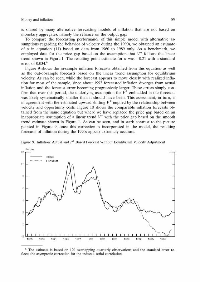
is shared by many alternative forecasting models of inflation that are not based onmonetary aggregates, namely the reliance on the output gap.
To compare the forecasting performance of this simple model with alternative as-sumptions regarding the behavior of velocity during the 1990s, we obtained an estimateof a in equation (11) based on data from 1960 to 1989 only. As a benchmark, weemployed data for the price gap based on the assumption that V* follows the lineartrend shown in Figure 1. The resulting point estimate for a was �0.21 with a standarderror of 0.034.6
Figure 9 shows the in-sample inflation forecasts obtained from this equation as wellas the out-of-sample forecasts based on the linear trend assumption for equilibriumvelocity. As can be seen, while the forecast appears to move closely with realized infla-tion for most of the sample, since about 1992 forecasted inflation diverges from actualinflation and the forecast error becoming progressively larger. These errors simply con-firm that over this period, the underlying assumption for V* embedded in the forecastswas likely systematically smaller than it should have been. This assessment, in turn, isin agreement with the estimated upward shifting V* implied by the relationship betweenvelocity and opportunity costs. Figure 10 shows the comparable inflation forecasts ob-tained from the same equation but where we have replaced the price gap based on aninappropriate assumption of a linear trend V* with the price gap based on the smoothtrend estimate shown in Figure 1. As can be seen, and in stark contrast to the picturepainted in Figure 9, once this correction is incorporated in the model, the resultingforecasts of inflation during the 1990s appear extremely accurate.
Money and inflation 89
Figure 9. Inflation: Actual and P* Based Forecast Without Equilibrium Velocity Adjustment
6 The estimate is based on 120 overlapping quarterly observations and the standard error re-flects the asymptotic correction for the induced serial correlation.

Figure 11 compares the two alternative forecasts shown in the two earlier figureswith a more realistic forecast meant to reflect more closely the information available inreal-time. In particular, the real-time forecast shown with the dash-dot line is based ona price gap, pt � p*t, that combines real-time measures of both an output gap and avelocity gap. The first observation, corresponding to the forecast of inflation ending in1993Q3, is based on real-time data capturing the four quarters ending in 1992Q3.Given the one-quarter lag in the publication of output data, this corresponds to infor-mation first available in 1992Q4. For the output gap, we use the estimate shown for thefiscal year 1992 as published at the time by the Congressional Budget Office.7, 8 For thevelocity gap, we rely on the reconstructed real-time estimates of the velocity gap shownin Figure 4. As can be seen, although the reconstructed real-time forecasts do notappear nearly as accurate as the ones based on the ex post characterizations of Q* andV* embedded in the smooth trend based forecasts, they are much closer to it thanforecasts obtained when the changes in the underlying trend of velocity is erroneouslyomitted.
One lesson that can be drawn from this experience is that although application ofthe P* model that failed to account for changes in the underlying equilibrium velocityof M2 during the 1990s could have easily provided misleading inflation forecasts, thisdifficulty was not nearly as important in practice as proper care could be taken toincorporate available information regarding the likely change of V*. As a result, proper
90 Athanasios Orphanides and Richard D. Porter
Figure 10. Inflation: Actual and P* Based Forecast
7 To be exact, this publication is typically available in January of the following year.8 This timing is determined by the availability of this real-time data. The Congressional Budget
Office publishes their estimates of historical output gaps on a fiscal year basis, which correspondsto a four-quarter average ending in the third quarter.

evaluation of whether money remained a useful indicator of inflation during this epi-sode or not hinges crucially on the appropriate treatment of information regarding thebehavior of velocity.
5. The influence of special factors
A central bank has access to a variety of information and analytical tools with which itcan sort out various movements in the aggregates. In particular, on a routine basis itmay be able to filter out high or low frequency movements in the aggregates that havenothing or very little to do with domestic activity or prices. From time to time suchfactors may be quite significant quantitatively. They could influence the growth rate ofnarrow monetary aggregates by several percentage points and could often influencethe quarterly growth rate of even a broad monetary aggregate such as M2 by over onepercentage point. Although judgmental interpretations of the information in monetaryaggregates routinely make allowances for such factors, simple time-series modelscannot systematically account for them. As a result, examination of the informationcontent of monetary aggregates based on traditional estimated time series models maysuggest that the aggregates are less useful than they truly are in practice, perhaps by aconsiderable margin. To illustrate this difficulty, in this section we offer some examplesof special factors that have been closely monitored at the Federal Reserve during the1990s.
Money and inflation 91
Figure 11. Inflation: Alternative P* Based Forecasts
Notes: The smooth and linear trend V* based forecasts correspond to those shown in Figure 1. Thereal-time forecast employs real-time estimates of the price gap, P� P*, based on the real-time (recur-sive) estimates of the velocity gap shown in Figure 4 and real-time estimates of the output gap. Eightobservations are shown corresponding to forecasts of inflation ending at the third quarter of eachyear from 1993 to 2000. These observations are connected with linear segments in the plot.

Two examples of major innovations that have affected the demand for the narrowaggregates in the United States during the 1990s are retail sweep programs at banksand large outflows of U.S. banknotes abroad. In 1994, falling costs of computing andprogramming made it practical for banks to begin to introduce retail sweep programsthat allowed them to profitably reduce the effective reserve requirements on individualhousehold accounts. In effect, this was achieved by transferring checkable deposits,which are subject to a reserve requirement tax, to money market deposit accounts,which are free of any such tax. At about the same time, events in Russia induced an-other distortion in the aggregates, massive currency outflows from the United States.Though by the early 1990s dollars already had a substantial foothold in Russia, theirusage grew significantly further during the period of rapid inflation, which occurred inthe middle of the decade. On average, Russians imported about $2 billion per month inU.S. currency from about 1994 to 1996, see Secretary of the Treasury (2000, p. 22).Over time, the combination of these two innovations greatly distorted the behavior ofthe currency to deposit ratio, a popular gauge used by Cagan (1958) and others as anindirect measure of underground activity. Porter and Weinbach (1999) show an adjustedratio that removes the effects of the two distorting influences–retail sweep programsand overseas demands for U.S. currency. The unadjusted ratio rises by over 60 percent,while the adjusted ratio falls. Indeed, movements in the adjusted ratio appear to belargely explained by the expected differential effects of interest rates on the compo-nents of the ratio, suggesting that there has not likely been a resurgence in under-ground activity in the United States.
More generally, the Federal Reserve has attempted to distinguish between move-ments in the aggregates that reflect sources of strength or weakness in underlying de-mands for the aggregate from other distortions that are either transitory in nature ordo not reflect such underlying demands, at least within the United States. Both sweepsand overseas currency outflows fall into the latter category, though only currency flowshave any effect on M2.9 In each case, Federal Reserve staff relies on independent dataseries to gauge the volume of the various distorting factors.
On balance, currency flows have tended to boost M2 but for reasons that have virtuallynothing to do with domestic output and prices, while sweeps have tended to lower M1 withno effect on M2. The effect on the level of M2 of such overseas holdings is perhaps as largeas $375 billion, or about 7-3/4 percent of the aggregate itself, Judson and Porter (2000).
Two other special factors that are routinely monitored at the Board involve tax pay-ments and mortgage refinancings, both of which may lead to distortions in the aggre-gates. Typically in April when individual tax payments are due, M2 surges as the cur-rent seasonals do not embody the outsized tax payments that come due and individualsmust boost their liquid balances prior to paying their taxes by more than ordinaryamounts. Estimates of these effects on M2 are made by drawing upon data on indivi-dual non-withheld tax receipts. The mortgage effects show up in the liquidation of mort-gage backed security (MBS) pools.
To illustrate, suppose longer-term interest rates fall sufficiently to reach a new lowerthreshold, which induces households in increasing numbers to refinance their mortgages
92 Athanasios Orphanides and Richard D. Porter
9 Estimates of currency abroad are published by the Board in its flow of funds accounts and bythe BEA in the International Investment Position of the United States on a quarterly basis, seeJudson and Porter (2000) and Secretary of the Treasury (2000).

to take advantage of the lower interest rates that now prevail, and the process triggersliquidation in a MBS pool. Regulations require that balances in the pool being liqui-dated be held in an account within M2 for up to seven weeks before the pool is paidout to investors, resulting in a temporary surge in the aggregate during this interval.Figure 12 shows a judgmental estimate of the contribution of such refinancings surgeson M2 growth in 1994 and 1995. When longer-term rates backed up in 1994, a declinein such refinancings was induced which contributed to an estimated 1-1/2 point declinein M2 by the middle of 1994.10 The effect was reversed later in the period, when ratesbegan to decline, setting off a massive surge in refinancings that boosted M2 in thelatter part of the period.
Some events occur that, in principle, one would wish to capture within the frame-work of a special factor decomposition (as is done for MBS effects, overseas currencyflows, sweeps, and tax effects) but are such that there is insufficient data to make anindependent quantitative assessment. A crisis that arose in the late summer and earlyfall of 1998 provides a striking illustration of this phenomenon. A worldwide crisisstruck capital markets after the Russian default in August and the subsequent difficul-ties at the hedge fund, Long Term Capital, emerged soon thereafter. The immediateeffect on global markets was to reduce the risk-bearing capacity of the system in partbecause of losses that had accrued and because of an apparent increased sensitivity to
Money and inflation 93
10 The bond rate shown is the monthly year-over-year change in the rate aggregated to a quar-terly frequency at which the MBS effect is also shown.
Figure 12. Mortgage Refinancing Activity and M2 Growth
Notes: The solid line indicates the percentage point change in the 10-year Treasury Bond Ratefrom four quarters earlier (left axis). The dotted line shows an estimate of the contribution ofmortgage refinancing activity to M2 growth during a quarter (right axis).

the attendant risks in the marketplace. The resulting distress spilled over to globalfinancial markets events and sparked a simultaneous large flight to quality and to li-quidity, which boosted liquid accounts in M2 drastically. M2 jumped from a 6.8 percentannual rate of growth in August to a 12.1 percent growth rate in September and accel-erated from a 7 percent annual rate in the third quarter to 10.7 percent in the fourthquarter of the year. On the credit side, funding shifted radically from the open capitalmarket to depositories, as turbulences in financial markets apparently altered financingterms and induced many firms to substitute bank loans for funds raised in markets.While these events in the latter half of 1998 were disruptive and led to a correctivemonetary policy reaction to restore confidence and liquidity in financial markets, theeffects on M2 were generally well understood contemporaneously. It was clear at thetime that the surge in M2 in the fall of 1998 largely represented just a shift in liquiditypreference with little likelihood of accelerating pressures on aggregate price measuresin the economy.
6. Conclusion
Interpreting the behavior of monetary aggregates involves a considerable degree ofjudgment and detailed analysis. Although it may be straightforward for central bankpractitioners to acquire the appropriate level of expertise to make sensible judgmentson these matters, it may be quite difficult, if not impossible, to quantify with muchprecision such judgments. Simple statistical techniques examining the usefulness ofmonetary aggregates as guides for inflation may fail to provide an accurate reading ofthis usefulness when information routinely available to monetary practitioners to screenspecial factors and detect changes in equilibrium velocity is not incorporated in theanalysis. However, central banks remain in a unique position to accumulate and inter-pret information regarding monetary aggregates. In light of the fundamental nature ofmoney growth for inflation, we believe that continued monitoring of the monetary ag-gregates remains well advised.
References
Cagan, Phillip, “The Demand for Currency Relative to the Total Money Supply”, Journal of Politi-cal Economy, 1958, 303–328.
Carlson, John B., Ben Craig and Jeffrey C. Schwartz, “Structural Uncertainty and BreakpointTests: An Application to Equilibrium Velocity”, Journal of Economics and Business, 52(1/2),101–115, January/April 2000.
Carlson, John B., Dennis L. Hoffman, Benjamin D. Keen and Robert H. Rasche, “Results of aStudy of the Stability of Cointegrating Relations Comprised of Broad Monetary Aggregates”,Journal of Monetary Economics, 46, 345–383, 2000.
Feinman, Joshua, and Richard D. Porter, “The Continuing Weakness in M2”, Federal ReserveBoard, Finance and Economics Discussion Series, No 209, September 1992.
Hallman, Jeffrey, Richard D. Porter, and David H. Small, “Is the Price Level Tied to the M2Monetary Aggregate in the Long-Run?”, American Economic Review, 841–858, September1991.
Judson, Ruth and Richard D. Porter, “Overseas Dollar Holdings: What Do we Know?” forthcom-ing in Wirtschafts Politische Blatter.
Lown, Cara, Stavros Peristiani, and Kenneth J. Robinson, “What Was Behind the M2 Break-down?” Federal Reserve Bank of Dallas, mimeo. 1999.
94 Athanasios Orphanides and Richard D. Porter

Orphanides, Athanasios and Richard D. Porter, “P* Revisited: Money-Based Inflation Forecastswith a Changing Equilibrium Velocity”, Journal of Economics and Business, 52(1/2), 87–100,January/April 2000.
Orphanides, Athanasios, Brian Reid and David H. Small, “The Empirical Properties of a MonetaryAggregate That Adds Bond and Stock Funds to M2”, The Federal Reserve Bank of St. LouisReview, 76(6) 31–51, November/December 1994.
Porter, Richard D. and Gretchen Weinbach, “Currency Ratios and U.S. Underground EconomicActivity,” Economic Letters, 63(3), 355–361, June 1999.
Secretary of the Treasury. The Use and Counterfeiting of United States Currency Abroad. Report tothe Congress in consultation with the Advanced Counterfeit Deterrence Steering Committee.Washington: U.S. Department of the Treasury, 2000.
Sephton, Peter, “Predicting Inflation Using MARS”, University of New Brunswick, mimeo, Sep-tember 2000.
Money and inflation 95


1. Introduction
Japan’s economy underwent an extremely severe recession in the years 1997 and 1998,which turned out to be the worst ever experienced by Japan in the postwar era. RealGDP recorded negative growth for five consecutive quarters from the fourth quarter of1997 on a quarter-to-quarter basis.1 This recession was largely influenced by the distur-bance in the financial system that occurred reflecting the failures of large financial insti-tutions from autumn 1997.2 As a result, several unusual phenomena were observed inthe business cycle. (See Chart 1)During the depressed phase of the economy from the end of 1997, for instance, the
financial system shock decreased private consumption by discouraging consumer senti-ment. Business fixed investment also declined substantially, especially at small firms,reflecting a decrease in the lending capacity of private banks. In particular, when globalconcern over credit risks was heightened in the second half of 1998, the deteriorationof the economy and tightening of financial conditions created a vicious cycle. Paradoxi-cally, however, the growth rate of money (particularly the monetary base) acceleratedamid the depressed real economy. On the other hand, the growth rate of money hasbeen slowing down gradually since 1999, while improvements have been observed inthe economy such as a recovery in industrial production and an improvement in corpo-rate sentiment. Thus, the relationship between money and income in recent years dif-fers from that depicted by orthodox economic theory .One explanation for this phenomenon is that mounting financial anxieties increased
precautionary demand for liquidity. The financial system shock caused fixed investment
The impact of financial anxietieson money demand in Japan*
Takeshi Kimura**
Bank of Japan
* This paper is a revised version of Kimura and Tanaka [1999] and Kimura and Fujita [1999].The author would like to gratefully acknowledge the useful comments on earlier versions of thepaper offered by members of the Bank of Japan’s Research and Statistics Department, especiallyHideo Hayakawa and Eiji Maeda. Helpful comments were also given by Christian Ølgaard andseminar participants at the European Central Bank. The opinions presented herein are the perso-nal views of the author, and do not represent the official opinion of the Bank of Japan or of thePolicy Planning Office.** Senior Economist, Policy Planning Office, Bank of Japan, Chuo-ku, Tokyo 103-0021.
E-mail: [email protected] This development of real GDP is based on 68SNA. (In October 2000, the data of real GDP
was revised to the new series, which is based on 93SNA.)2 See Hayakawa and Maeda [2000] for a survey on Japan’s Financial and Economic Develop-
ments since autumn 1997.

98 Takeshi Kimura
Chart 1. Money

and private consumption to decrease, and simultaneously caused the precautionary de-mand for money to increase significantly from the end of 1997 to 1998. On the otherhand, since 1999, easing anxieties over the financial system have resulted in the recov-ery of the economy, but the growth rate of money has been moderated by a decreasein precautionary demand. The empirical analysis in the following sections supportsthese interpretations.Following this Introduction, in order to investigate the extent of the impact from
the financial system shock, Section 2 presents a time series model and tests the stabi-lity of the model. The results demonstrate that the financial system shock in autumn1997 was substantial enough to break the long-run equilibrium relationship that hadexisted among economic variables, especially the relationship between money andincome. Section 3 quantifies financial anxieties as a proxy for the precautionary de-mand for money, and incorporates this proxy into the model. The results demon-strate that taking the precautionary demand for money properly into account in themoney demand function leads to a stable relationship between money and income,even when including the years 1998 and 1999. Section 4 uses the conventional IS-LManalysis framework and simulates the estimated model to consider how the financialsystem shock influenced Japan’s economy after autumn 1997 and how the policiestaken in those circumstances can be evaluated. Finally, Section 5 provides a briefconclusion.
2. Magnitude of the financial system shock
In this section, in order to examine the impact of the financial system shock on Japan’seconomy, I specify the following vector error correction model (VECM) for seven ma-jor economic variables, and test the stability of the model.
DXt ¼ GðLÞ DXt þ PXt�1 þ mt ; ð1Þ
where Xt is the vector of the seven variables, M2 + CDs, monetary base, real GDP,CPI, stock prices (Nikkei 225), long-term interest rates, and short-term interest rates.GðLÞ is a coefficient matrix for a k-th order lag process. The hypothesis of cointegrationis expressed as a reduced rank of the matrix P(7 � 7):
H0(r) : P ¼ ab0 ; (2)
where b0 is an (r � 7) matrix of r cointegrating vectors and a is a (7 � r) matrix ofloading vectors. b0Xt are the so-called cointegrating relations.Cointegration tests are obtained using Johansen’s [1988] trace statistic, estimated
from the VECM with lag-length k = 2. I estimate the model over the two periods 1977/1Q–1997/3Q and 1977/1Q–1998/3Q to examine the impact of the financial systemshock that occurred in autumn 1997.3, 4
The impact of financial anxieties on money demand in Japan 99
3 The sample period is chosen to avoid the high inflation period of the first-round increases inoil prices, since the expectation formation process of the private sector may have changed aftertransition to a moderate or low inflation period.
4 The analysis in Section 2 is based on Kimura and Tanaka [1999], which was written in Febru-ary 1999. When that paper was written, the data for 1998/4Q and after were not available. Hence,the end of the sample period is set to 1998/3Q.

The estimation results are shown in Chart 2. While the trace statistic indicates thatthere are five cointegrating relations over the period 1977/1Q–1997/3Q at the 5% sig-nificance level, the number of cointegrating relations decreases from five to three whenthe sample for 1998 is included.5 This suggests that some of the long-run equilibrium
100 Takeshi Kimura
Chart 2. Magnitude of Financial System Shock
5 Over the period 1977/1Q–1997/3Q, it is possible to make natural economic interpretations forfive cointegrating relations, that is, (1) the money demand function, (2) the money multiplier, (3)
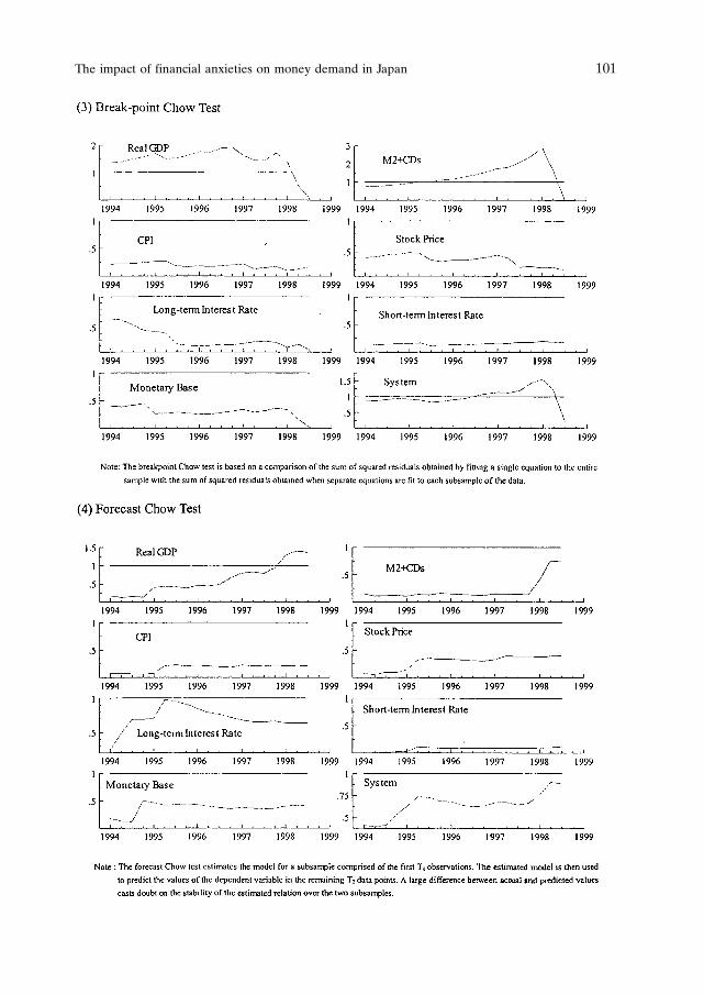
The impact of financial anxieties on money demand in Japan 101

relationships between economic variables broke down in 1998. In addition to cointegra-tion tests, I conduct three kinds of Chow tests to confirm the stability of the model. Theresults of the Chow tests indicate that the parameters of both real GDP and M2 + CDsequations become unstable in 1998.6
These results imply that the financial system shock in autumn 1997 was substantialenough to break the long-run equilibrium relationship that had existed among econom-ic variables, especially between money and income. In order to deepen our understand-ing of the impact of the financial system shock, we need to analyze the relationshipbetween money and income in more detail.
3. Cointegration analysis of money and income
In the following analysis, for the simplicity of the model, I focus not on the relationshipamong the seven economic variables, but only on the relationship between real moneyand real GDP.I postulate the VECM as follows:
Drmt ¼ amECt�1 þPki¼1
gmi Drmt�i þPki¼1
qmi Dyt�i þPki¼0
lmi Drst�i
þPki¼0
rmi DRt�i þ cm þ "t ð3Þ
Dyt ¼ ayECt�1 þPki¼1
gyi Drmt�i þ
Pki¼1
qyi Dyt�i þ
Pki¼0
lyi Drst�i
þPki¼0
ryi DRt�i þ cy þ dt ð4Þ
ECt ¼ rmt � byyt � bsrst ð5Þ
where rmt, yt, rst, Rt are the real money stock (M2+CDs deflated by the GDP deflator),real GDP, real stock prices (Nikkei 225 deflated by the GDP deflator) and long-terminterest rates, respectively. cm and cy are constant terms, and et and dt are error terms.The reason why real stock prices are included as an exogenous variable in (3)–(5) is tocontrol the wealth effect in money demand.7
102 Takeshi Kimura
the Fisher relation, (4) the term structure spread linking the short-term rate and the long-termrate, and (5) the stable relationship between nominal GDP and stock prices. The parameter con-straints which satisfy the above five relations cannot be rejected at the 5% significance level. (Theestimation results are omitted.) However, a natural economic interpretation cannot be made re-garding the three cointegrating relations for the period 1977/1Q–1998/3Q.
6 The breakpoint Chow test for the real GDP equation indicates that the null hypothesis on thestability of the parameter can be rejected for the sample period 1994/1Q–1998/1Q. This resultmeans that there was a breakdown in the real GDP relation somewhere between 1994/1Q and1998/1Q, since the breakpoint Chow test is based on a comparison of the entire sample (in this case1977/1Q–1998/3Q) with the subsample whose staring point is 1977/1Q. With the breakpoint Chowtest, we cannot specify the timing of the breakdown in the real GDP relation, but we can concludethat it was 1998/1Q based on the results of the one-step Chow test and the forecast Chow test.
7 It is very important to take asset prices into account in estimating Japan’s money demandfunction, because Japan experienced the bubble economy in the late 1980s and the bursting of thebubble in the early 1990s.

ECt in equation (5) is an error correction term, which represents the deviation fromthe long-run equilibrium relationship among real money, real GDP and real stockprices.8 The expected sign of the loading vector is negative for am, and positive for ay.
3.1. Estimation Results
Cointegration tests are conducted using Johansen’s [1988] maximal eigenvalue statisticand trace statistic, estimated from the VECM. I estimate the model over the two peri-ods 1980/1Q–1997/3Q and 1980/1Q–1991/1Q to focus on the impact of the financialsystem shock that occurred in autumn 1997 on money demand.9
The estimation results are presented in Chart 3. The results show that the cointegrat-ing relationship between real money and real income exists for the sample period 1980/1Q–1997/3Q and that the loading vector (am, ay) is of the right sign.10 On the contrary,when extending the sample period up to 1999/1Q, it is no longer possible to reject thenull hypothesis that there is no cointegration.Why does the inclusion of the recent sample result in the breakdown of the long-run
equilibrium relationship? I hypothesize that this is because the model ignores the im-pact of financial system shock. The financial system shock increased the uncertainty offuture financing in the private sector, which led to an increase in the precautionarydemand for money as well as a decrease in private sector expenditures. Because theimpact of the financial system shock was very large, as shown in Section 2, ignoring therise in the precautionary demand for money in the model (3)–(5) means the missingvariable in the VECM. A natural strategy for resolving this problem is to quantify thefinancial anxieties as a proxy for the precautionary demand and to incorporate this intothe VECM.
The impact of financial anxieties on money demand in Japan 103
8 The long-run equilibrium relationship between money and income is based on the quantitytheory of money.
9 The analysis in Section 3 is based on Kimura and Fujita [1999]. When that paper was written, thedata for 1999/2Q and after were not available. Hence, the end of the sample period is set to 1999/1Q.
10 Income elasticity by is around 1.5. Income elasticity above unity is consistent with the ob-served upward trend in the Marshallian k. (See Chart 1.)
Sampleperiod
Johansen’s Cointegration Test Cointegrating vector Loading vector
Maximaleigenvalue statistic
Trace statistic by bs am ay
80/1Q–97/3Q 16.37*(14.10)
20.23**(15.40)
1.451(0.032)
0.076(0.012)
–0.101(0.072)
0.245(0.079)
80/1Q–99/1Q 8.61(14.10)
11.52(15.40)
1.595(0.079)
0.032(0.031)
0.000(0.039)
0.136(0.049)
Notes: 1. Values in parentheses in the “Johansen’s Cointegration Test” columns are critical values at the 5%significance level. ** indicates rejection of the null hypothesis (= there is no cointegration) at the 1%significance level and * indicates rejection of the null hypothesis at the 5% significance level.
2. Values in parentheses in the “Cointegrating vector” and “Loading vector” columns are standard errorsfor the estimated parameters.
3. The lag-length of the VECM is set to 3 (k = 3), obtained from the likelihood-ratio test.
Chart 3. Cointegation Analysis of Money and Income (without taking financial anxieties into account)

3.2. Quantification of financial anxieties
Although it is difficult to quantify unobservable financial anxieties, they are estimatedhere using the Corporate Financial Position Diffusion Index from the Bank of Japan’sTankan – Short-term Economic Survey of Enterprises. The Financial Position DI de-pends roughly on the interest rate on loans (See Chart 4). Hence, I postulate this rela-tionship as the following equation.
DIt ¼ b0 þ b1 ratet þ b2 ratet�1 þ "t ; ð6Þ
where DIt, and ratet are the diffusion indexes for the financial position of firms (“easy”minus “tight”) and the interest rates on loans (“rise” minus “fall”), respectively. et is anerror term, which represents the influence of irregular or unexpected factors other thaninterest rates on loans. We can regard the variance of this error term as the uncertaintyof financing (i.e. financial anxieties). Even when the interest rate on loans is constant,the financial position may change due to financial anxieties. Such a phenomenon can berepresented as a time-varying variance, and in order to take it into account I estimateequation (6) by using the following TARCH (Threshold AutoRegressive ConditionalHeteroscedasticity) model.
"t j It�1 Nð0; h2t Þ ; h2t ¼ ao þ a1"2t�1 þ a2"
2t�1dt�1 þ a3h
2t�1 ; ð7Þ
where It�1 is the information set available at period t � 1.
dt is a dummy variable. dt ¼1 ; if "t < 0
0 ; if "t 0:
�
104 Takeshi Kimura
Chart 4. Diffusion Indexes for the Financial Position of Firms and the Interest Rate on Loans
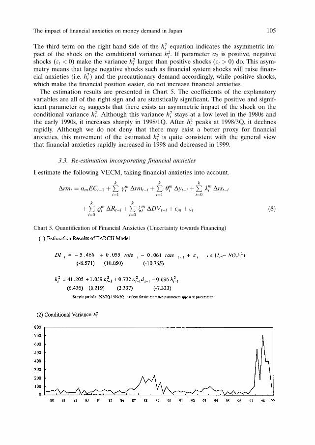
The third term on the right-hand side of the h2t equation indicates the asymmetric im-pact of the shock on the conditional variance h2t . If parameter a2 is positive, negativeshocks ("t < 0) make the variance h2t larger than positive shocks ("t > 0) do. This asym-metry means that large negative shocks such as financial system shocks will raise finan-cial anxieties (i.e. h2t ) and the precautionary demand accordingly, while positive shocks,which make the financial position easier, do not increase financial anxieties.The estimation results are presented in Chart 5. The coefficients of the explanatory
variables are all of the right sign and are statistically significant. The positive and signif-icant parameter a2 suggests that there exists an asymmetric impact of the shock on theconditional variance h2t . Although this variance h2t stays at a low level in the 1980s andthe early 1990s, it increases sharply in 1998/1Q. After h2t peaks at 1998/3Q, it declinesrapidly. Although we do not deny that there may exist a better proxy for financialanxieties, this movement of the estimated h2t is quite consistent with the general viewthat financial anxieties rapidly increased in 1998 and decreased in 1999.
3.3. Re-estimation incorporating financial anxieties
I estimate the following VECM, taking financial anxieties into account.
Drmt ¼ amECt�1 þPki¼1
gmi Drmt�i þPki¼1
qmi Dyt�i þPki¼0
lmi Drst�i
þPki¼0
rmi DRt�i þPki¼0
zmi DDVt�i þ cm þ "t ð8Þ
The impact of financial anxieties on money demand in Japan 105
Chart 5. Quantification of Financial Anxieties (Uncertainty towards Financing)

Dyt ¼ ayECt�1 þPki¼1
gyi Drmt�i þPki¼1
qyi Dyt�i þPki¼0
lyi Drst�i
þPki¼0
ryi DRt�i þPki¼0
zyi DDVt�i þ cy þ dt ð9Þ
ECt ¼ rmt � byyt � bsrst � bDDVt ; ð10Þ
where DVt is the conditional variance h2t shown in Chart 5. The expected sign of bD,the coefficient of DVt in equation (10), is positive, because financial anxieties (i.e. therise in DVt) make the precautionary demand for money increase.
106 Takeshi Kimura
(1) Cointegration Test
Sampleperiod
Johansen’s Cointegration Test Cointegrating vector Loading vector
Maximal eigen-value statistic
Tracestatistic
by bs bD am ay
80/1Q–97/3Q 16.59*(14.10)
20.28*(15.40)
1.458(0.038)
0.072(0.017)
0.415(1.199)
–0.097(0.072)
0.247(0.080)
80/1Q–99/1Q 17.68*(14.10)
21.25**(15.40)
1.498(0.036)
0.053(0.014)
1.721(0.637)
–0.080(0.063)
0.236(0.069)
Notes: 1. Values in parentheses in the “Johansen’s Cointegration Test” columns are critical values at the 5%significance level. ** indicates rejection of the null hypothesis (= there is no cointegration) at the 1%significance level and * indicates rejection of the null hypothesis at the 5% significance level.
2. Values in parentheses in the “Cointegrating vector” and “Loading vector” columns are standard errorsfor the estimated parameters.
3. The lag-length of the VECM is set to 3 (k = 3), obtained from the likelihood-ratio test.4. The cointegration Vector bD and its standard error are shown multiplied by 10000 times.
Chart 6. Cointegation Analysis of Money and Income (with taking financial anxieties into account)
(2) Money Gap adjusted for the Precautionary Demand for Money
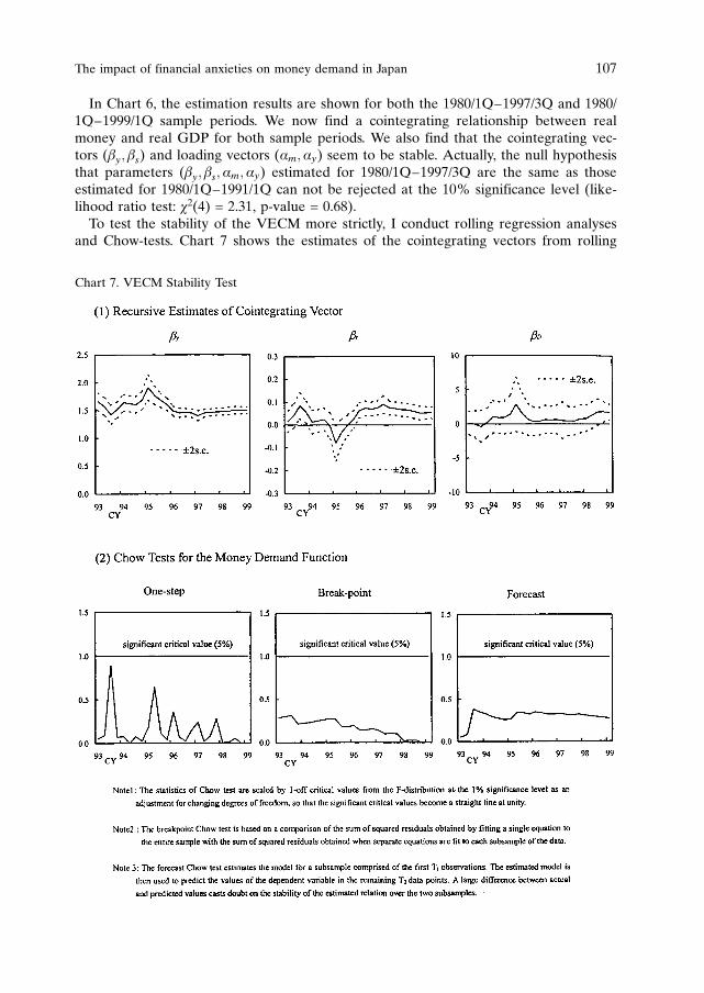
In Chart 6, the estimation results are shown for both the 1980/1Q–1997/3Q and 1980/1Q–1999/1Q sample periods. We now find a cointegrating relationship between realmoney and real GDP for both sample periods. We also find that the cointegrating vec-tors (by; bs) and loading vectors (am;ay) seem to be stable. Actually, the null hypothesisthat parameters (by; bs;am;ay) estimated for 1980/1Q–1997/3Q are the same as thoseestimated for 1980/1Q–1991/1Q can not be rejected at the 10% significance level (like-lihood ratio test: c2(4) = 2.31, p-value = 0.68).To test the stability of the VECM more strictly, I conduct rolling regression analyses
and Chow-tests. Chart 7 shows the estimates of the cointegrating vectors from rolling
The impact of financial anxieties on money demand in Japan 107
Chart 7. VECM Stability Test

regressions with the horizontal axis showing the end of sample for each regression.11
The results show that by and bs have remained stable since 1996.12 Moreover, the threekinds of Chow tests suggest that all the parameters of the money demand function (8)remained stable in the 1990s.In this way, the long-run equilibrium relationship between money and income re-
mains stable even when the recent sample period is included in the VECM. This isbecause the revised model properly takes into account the impact of the financial anxi-eties on money demand.
3.4. Evaluation of the money gap
The lower figure of Chart 6 shows the money gap, that is, the gap between equilibriumand actual money stock, which is indicated by ECt in equation (10). Although themoney gap without adjustment for precautionary demand shows a wide spread from1998, that adjusted for precautionary demand was around zero during 1998, and thenexpanded widely from the beginning of 1999.In this sense, taking the precautionary demand properly into account, we can con-
clude that the monetary conditions were not easy but rather just at equilibrium in 1998,even though the growth rate of money and the Marshallian k increased rapidly in 1998(See Chart 1.).13 From 1999, monetary conditions finally became easy, even though thegrowth rate of money began to decrease in 1999.
4. Theoretical framework for the impact of financial system shockon money and income
On the basis of the empirical analysis above, let us now consider how financial systemshock influenced Japan’s economy after autumn 1997 and how the policies taken inthose circumstances can be evaluated, using the conventional IS-LM analysis frame-work (Chart 8).
(a) Financial system shock exerts a negative impact on business fixed investment andprivate consumption, shifting the IS curve to the left.14 At the same time, financialsystem shock creates a precautionary demand for money, which means heightenedliquidity preference, thus increasing the demand for money under constant GDP.
108 Takeshi Kimura
11 The starting point of the regressions is fixed at 1980/1Q.12 It is not until 1998 that parameter bD becomes significant, but this does not imply the instabil-
ity of bD. It just means that before 1997 we cannot estimate the impact of financial anxieties onmoney demand precisely, because in that period DVt hardly changes.
13 The increase in money was attributed to the following two factors: (i) there was a shift offunds from financial assets not included in M2+CDs, such as investment trusts and bank deben-tures, to bank deposits with higher liquidity, due to rising anxieties over the financial system; (ii)some firms gathered a large amount of on-hand funds (deposits) by issuing CP (Commercial Pa-per) and borrowing from banks due to concerns about the future availability of funds. Also therise in the monetary base is due to an increase in cash demand in line with financial anxiety, andthe accumulation of reserves by financial institutions in preparation for unexpected account with-drawals and fund-raising difficulties in the market. Thus, the growth rate of money increased,although the transaction demand for money declined as the economy receded.
14 Financial system shock may also make the IS curve steeper, which means that investmentbecomes less sensitive to changes in interest rates.

The impact of financial anxieties on money demand in Japan 109
Chart 8. Impact of Financial System Shock (IS-LM Framework)
This leads to a rise in interest rates under constant money supply, that is, a shift ofthe LM curve to the left. In other words, the financial system shock brings about“an unintended monetary tightening” under constant money growth. As a result ofthese leftward shifts of both the IS and LM curves, the real economy contractssignificantly.
(b) The hypothesis that there was a substantial leftward shift of the LM curve is consis-tent with the upward pressure on interest rates on term instruments after the finan-cial system shock and the tightening of corporate finance, particularly in the secondhalf of 1998.15, 16 The Bank of Japan attempted to prevent the leftward shift of theLM curve by providing ample funds.17 This can be confirmed by the fact that themoney gap, adjusted for precautionary demand, did not contract but was at equili-brium on the whole during 1998. That is, the ample supply of funds by the Bankavoided a drastic increase in interest rates on term instruments, and then led to thehigher growth of money.
(c) After 1999, the LM curve at last shifted to the right owing to the zero interest ratepolicy implemented from February 199918 and the easing of financial anxiety reflect-ing the injection of public funds.19, 20 This point can be confirmed by the fact thatthe adjusted money gap became wide in 1999. This means that the effects of mone-tary easing permeated further or were fully manifest. Also, in this process, the de-cline in interest rates on term instruments and the slowdown of the money growthrate occurred simultaneously, due to the decrease in the precautionary demand formoney.
110 Takeshi Kimura
15 After autumn 1997, the degree of the leftward shift pressure of the LM curve was larger thanthat of the IS curve, resulting in upward pressure on interest rates.
16 In the financial market, there was upward pressure on funding costs for the private sector.Interest rates on term instruments such as three-month Euro-yen rates and yields on bank deben-tures rose through the beginning of 1998. Yields on corporate bonds with low ratings also rose. Asfor short-term funds, the differential between Euro-yen and TB (Treasury Bills) interest rates ex-panded to around 1 percent at the end of 1997, after the failures of major financial institutionswere revealed. The so-called Japan Premium (a premium imposed on Japanese banks when raisingfunds in U.S. dollars) also increased substantially.
17 The Bank of Japan encouraged a lowering of interest rates on term instruments and tried tofacilitate corporate finance by conducting longer-term operations to provide funds maturing afterthe fiscal year-end. In September 1998, the Bank decided to further ease its monetary policy. Thiswas done by lowering the overnight call rate to “around 0.25 percent” from levels “around slightlybelow the official discount rate (0.5 percent).” Then, in November the Bank decided to adopt thefollowing three policies in order to alleviate corporate financial conditions: (i) expansion of CPrepo operations; (ii) establishment of a temporary lending facility to support firms’ financing activ-ities; (iii) establishment of a new market operation scheme which utilizes corporate debt obliga-tions as eligible collateral.
18 The Bank of Japan, at the Monetary Policy Meeting on February 12, decided to further easeits policy stance by encouraging the uncollateralized overnight call rate, which had been aroundthe 0.25 percent level, to move as low as possible. This monetary easing was decided so as to“avoid possible intensification of deflationary pressure and to ensure that the economic downturnwill come to a halt.” Along with the further supply of ample funds, the overnight call rate declined,gradually dropping to zero by mid-March.
19 The government injected a total of 7.5 trillion yen worth of public funds into 15 major banksat the end of March.
20 The IS curve also shifted back to the right to some extent, in line with easing financial anx-iety. An increase in public expenditures was also a factor in the rightward shift of the IS curve.

To quantify these interpretations, I conduct a simulation in which the financial systemshock (i.e. financial anxieties) is incorporated into the VECM estimated in Section 3,assuming that this shock would dissipate completely after two years. The results are asfollows (Chart 9):
(a) The financial system shock pushes down GDP at the beginning (leftward shift ofthe IS curve), and it simultaneously causes the precautionary demand for money toincrease substantially, pushing down the adjusted money gap (shortage of money,large leftward shift of the LM curve).
(b) As a result of the decrease in the money gap (disequilibrium), such forces work torestore the equilibrium. That is, they push GDP further down and increase realmoney (rise in the Marshallian k).
(c) About a year later, as the precautionary demand for money decreases due to eas-ing anxieties about the financial system, the money gap comes to surpass the base-line (excess money, rightward shift of the LM curve).
(d) While excess money along with the decreased uncertainty leads to an increase inreal GDP, real money itself turns to a decrease (decline in the Marshallian k).21
(e) GDP surpasses the baseline after about two years.
It should be emphasized that the simulation results do not necessarily guarantee asteady economic recovery, since they are based on various assumptions.22 The results,however, provide a useful framework to understand that the real economy and moneymay move in opposite directions with the outbreak and ease of financial system shock.On the basis of these results, it is important to recognize that money growth may slowduring economic recovery, if the economy recovers as a result of easing financial anxi-eties. After the currency crisis in November 1997, Korea also underwent a recessionaccompanied by a disturbance in the financial system. In that case, the economy wasdepressed even though money growth rose, but as financial anxieties eased graduallyfrom the start of 1999, the economy has recovered notably while money growth hasslowed (Chart 10). This observation supports the above view that financial systemshocks change the orthodox relationship between money and the economy.I would also point out that, in a situation where money demand becomes extremely
volatile due to financial system shocks, interest rates rather than money stock should betargeted to implement monetary policy, as the classical paper by Poole [1970] showedthirty years ago. When the money demand becomes extremely volatile (i.e., the LMshock is extremely large), there is a high possibility that interest rates will rise signifi-cantly and damage the economy when keeping money growth constant. Furthermore,since it is difficult to quantify and forecast the extent to which such a shock fluctuatesthe demand for money, setting a proper target for money becomes an extremely toughtask. Therefore, we may conclude that a policy that focuses on interest rates and pro-motes their decline is preferable.
The impact of financial anxieties on money demand in Japan 111
21 A positive money gap leads to an increase in real GDP and a decrease in real money. Thelatter is caused by either a decrease in nominal money or rises in price levels. In Appendix, Iestimate the P* model of inflation to investigate the impact of the money gap on the price level.
22 In addition, under the conditions in which various structural problems exist and corporaterestructuring exerts downward pressure on the economy, the effects of monetary easing alone can-not bring about a self-sustaining recovery led by private demand.

112 Takeshi Kimura
Chart 9. Impact of Financial System Shock (VECM Dynamic Simulation)

The impact of financial anxieties on money demand in Japan 113
Chart 10. Money Stock and GDP (Korea)

5. Concluding remarks
This paper has examined Japan’s financial and economic developments after the finan-cial system shock in autumn 1997, and the findings may be summarized as follows:
(a) Developments in the real economy have had strong interactions with financial de-velopments since the financial system shock occurred in autumn 1997. In particular,when global concern over credit risks was heightened in the second half of 1998,the deterioration of the economy and tightening of financial conditions created avicious cycle. Since the beginning of 1999, the opposite developments have beenobserved due to an easing of financial anxiety.
(b) Looking at the relationship between money and the economy during this period,the growth rate of money increased while the real economy became depressed dur-ing 1998, but it started to decelerate as the economy began picking up in 1999.Thus, in the last three years, money and the economy have shown a relationshipthat is significantly different from the traditional one.
(c) This relationship has been influenced by the rise and fall in the precautionary de-mand for money along with the mounting and easing of financial anxiety.
(d) In terms of monetary policy, the Bank of Japan supplied ample funds to meet theincrease in precautionary demand and tried to suppress overall interest rates during1998. In 1999, precautionary demand declined as financial anxiety receded and theBank continued to supply additional ample funds. As a result, interest rates de-creased further and various risk premiums also contracted in the financial market.Thus, the effects of monetary easing became full-scale.
Appendix: Estimation of the P* model of inflation
The simulation in Section 4 suggests that a positive money gap will lead to an increasein real GDP and a decrease in real money. The latter is caused by either a decrease innominal money or a rise in price levels. In this appendix, I estimate the P* model ofinflation to investigate the impact of the money gap on price levels.I modify the original P* model, which was proposed by Hallman, Porter and Small
[1991], by following Atta-Mensah [1996]. The form of regression is:
pkt ¼ aMGt�k þ bGGt�k þ gIPIkt þ qpkt�k þ cþ mt ðA1Þ
ptk is the annualized k-quarter growth rate of prices. This is defined as:
pkt ¼ ½log ðptÞ � log ðpt�kÞ� � 400=k ; ðA2Þ
where k is the quarter (1,4,6,8) and pt is the price level (CPI and the GDP deflator).23
MGt is the money gap created from equation (10), that is, the error correction termECt. GGt is the GDP gap estimated using a Cobb-Douglas type production function.IPItk is the annualized k-quarter growth rate of import prices, which is defined similarlyby equation (A2).24 I assume that the error term mt follows MA (k� 1) process, be-cause the overlapping data generate a moving-average error of order k� 1.
114 Takeshi Kimura
23 The price index is seasonally adjusted by X-12-ARIMA.24 When using the GDP deflator as the dependent variable, I exclude IPIt from the model,
since the GDP deflator can be regarded as home-made inflation.

The impact of financial anxieties on money demand in Japan 115
(1) CPI Model
Parameter ofMoney GAP
a
Parameter ofGDP GAP
b
Parameter ofImport Price
g
Parameter ofOwn Lag
q
AdjR2 SE (%)
k = 1 0.040(0.636)
0.188(2.454)
0.012(2.007)
0.639(8.565)
0.677 1.047
k = 4 0.055(2.873)
0.224(5.529)
0.022(4.452)
0.364(7.508)
0.949 0.294
k = 6 0.118(4.611)
0.296(6.745)
0.024(4.441)
0.278(5.495)
0.953 0.256
k = 8 0.003(0.364)
0.123(3.155)
0.023(2.537)
0.522(5.382)
0.959 0.217
(2) GDP Deflator Model [g = 0]
Parameter ofMoney GAP
a
Parameter ofGDP GAP
b
Parameter ofOwn Lag
q
AdjR2 SE (%)
k = 1 0.138(1.434)
0.443(4.090)
0.357(3.567)
0.413 1.618
k = 4 0.124(3.009)
0.419(5.938)
0.160(2.177)
0.888 0.485
k = 6 0.179(4.734)
0.440(6.401)
0.145(1.930)
0.908 0.394
k = 8 0.135(3.823)
0.338(4.855)
0.200(1.755)
0.926 0.328
Note 1. Sample period is 1980/1Q–1999/1Q.2. Values in parentheses are t-values.
(3) Forecast Perfomance (Unit: %)
CPI Model GDP Deflator Model
RMSE MAE RMSE MAE
k = 1k = 4k = 6k = 8
0.7660.3580.3020.531
0.5940.2820.2490.405
1.6210.5880.6000.714
1.2650.4630.4580.632
Note: Suppose the forecast sample is t = S, S + 1, S + h and denote the actualand forecast value in period t as pkt ; ppkt , respectively.Then, RMSE and MAE are computed as follows:
RMSE ðRoot Mean Squared ErrorÞ ¼
ffiffiffiffiffiffiffiffiffiffiffiffiffiffiffiffiffiffiffiffiffiffiffiffiffiffiffiffiffiffiffiffiffiffiffiffiffiffiffiffiffiffi1
hþ 1
PSþht¼S
ðppkt � pkt Þ2
s
MAE ðMean Absolute ErrorÞ ¼ 1hþ 1
PSþht¼S
jppkt � pkr j
Chart 11. Estimation Results of P* Model
The estimation results are shown in Chart 11. The sample period for the estimation is1980/1Q–1999/1Q, which is same as in Section 3. The coefficient of the GDP gap isfound to be statistically significant at the one- to eight-quarter horizon for both the CPImodel and the GDP deflator model. While the coefficient of money gap is not statisti-cally significant at the one-quarter horizon for both models, it is significant at the four-and six-quarter horizons for the CPI model and at the four- to eight-quarter horizonsfor the GDP deflator model. The coefficient of the money gap is the largest at the six-quarter horizon for both models.I also examine the out-of-sample forecasting performance of the modified P* model
and calculate the root-mean-square error (RMSE) and mean absolute error (MAE).25
According to these criteria, the out-of-sample forecast performance of both models isreasonably good at the six-quarter horizon.Thus, these estimation results suggest that the money gap is useful for forecasting the
inflation rate at the six-quarter horizon, although we need more time and data to con-clude that money remains to be an useful information variable under low inflation.
References
Atta-Mensah, Joseph, “A Modified P*-Model of Inflation Based on M1”, Bank of Canada, Work-ing Paper 96-15, November 1996.
Johansen, Soren, “Statistical Analysis of Cointegrating Vectors”, Journal of Economic Dynamicsand Control, 12, 1988, pp. 231–254.
Kimura, Takeshi and Hidenori Tanaka, “Suyou Keizaihensuu kan no Sougo-izon-kankei no Fuan-teisei” (The Instability of the Relationships between Main Economic Indicators; available inJapanese only), Research and Statistics Department, Bank of Japan, mimeo, February 1999.
Kimura, Takeshi and Shigeru Fujita, “Kinyufuan to Mane, Jittaikeizai, Bukka no Kankei ni tsuite”(The impact of Financial Anxieties on Money, the Real Economy, and Prices; available in Japa-nese only), Research and Statistics Department, Bank of Japan, Working Paper Series 99-6,December 1999.
Hayakawa, Hideo and Eiji Maeda, “Understanding Japan’s Financial and Economic Developmentssince Autumn 1997”, Research and Statistics Department, Bank of Japan, Working Paper Series00-1, January 2000.
Hallman, J., R. Porter and D. Small., “Is the Price Level Tied to the M2 Monetary Aggregate inthe Long Run?”, American Economic Review 81, 1991, pp. 841–858.
Poole, William, “Optimal Choice of Monetary Policy Instrument in a Simple Stochastic MacroModel”, Quarterly Journal of Economics 84, May 1970, pp. 197–216.
116 Takeshi Kimura
25 The predictive performance of the models is assessed by running recursive regressions overthe sample period. This method involves the estimation of the model from 1980/Q1 to 1995/Q1and a k-quarter-ahead forecast, where k=1,4,6 and 8. The models are re-estimated by extendingthe sample size by a quarter at a time and k-quarter-ahead forecasts are made each time. Theprocess continues until the data points are exhausted.

1. Introduction
In October 1998, the Governing Council of the ECB announced the main elements ofits monetary policy strategy.First, it provided a quantitative definition of the primary objective of monetary policy
in the euro area, namely price stability. Price stability was defined as an annual increasein the Harmonised Index of Consumer Prices (HICP) for the euro area of below 2%.Second, the Governing Council defined a framework for structuring the analysis
and assessment of economic data which underlies monetary policy decisions. In recog-nition of the fundamentally monetary nature of inflation over the medium term, theECB assigned a prominent role to money in the formulation of policy decisionsaimed at the maintenance of price stability. This “first pillar” of the strategy wassignalled by the announcement of a quantitative reference value for monetary growth.Moreover, acknowledging the influence of non-monetary factors on price develop-ments and recognising the important information relevant for monetary policy deci-sions contained in other indicators, the ECB announced that, in addition to a thor-ough analysis of monetary developments, a broadly based assessment of a wide rangeof other economic and financial variables would also be undertaken and constitute afurther basis for monetary policy decisions. This assessment is labelled the “secondpillar” of the strategy.This paper describes the framework and tools of monetary analysis from the point
of view of ECB staff. It explains in more detail some of the tools and approacheswhich are used by ECB staff for monetary analysis under the “first pillar” and otherswhich are under development or may be used in the future. The remainder of thepaper is organised as follows. Section 2 recalls some general issues underlying thestrategy as a whole. Against this background, Section 3 outlines the main arguments
Framework and tools of monetary analysis
Klaus Masuch, Huw Pill and Caroline Willeke*
European Central Bank
* The authors of this paper are staff members of the Directorate Monetary Policy in the Direc-torate General Economics of the European Central Bank (ECB). (Since the paper was finalised,Huw Pill has moved to the Graduate School of Business Administration, Harvard University). Thecontents of this paper represent the views of the authors and not necessarily those of either theECB or the Eurosystem. It has benefited from the comments of our discussant, H. Dillen ofSveriges Riksbank, other participants in the workshop and our colleagues at the ECB, in particularP. Moutot, H.-J. Klockers, J.-L. Escriva, S. Nicoletti Altimari, C. Brand and A. Calza. The underly-ing analysis and tools presented in the paper are based on the collective work of the staff of theDirectorate Monetary Policy at the ECB.

for assigning a prominent role to money in the strategy and briefly describes thegeneral role of the quantitative reference value for monetary growth. Section 4 dis-cusses the features of the regular monitoring of various monetary aggregates andtheir components and counterparts. Section 5 describes various tools and conceptsbased on money demand models which may contribute to deriving the informationcontent of monetary aggregates for monetary policy. Section 6 provides some evi-dence regarding the information content of monetary aggregates for future price de-velopments and discusses the uses and limitations of money-based projections. Section7 briefly concludes.
2. General strategic issues
Before turning to a description of the role of monetary analysis in the ECB’s strategy,it is worth making a number of more general observations regarding the strategy. Inparticular, several common misconceptions should be clarified.First, the ECB’s strategy is often misunderstood by external observers as implying
multiple targets for monetary policy. On the one hand, the prominent role for money isassociated with an intermediate monetary target, whereas, on the other hand, the “sec-ond pillar” is often characterised as a direct inflation target.However, at the outset it should be emphasised that the maintenance of price sta-
bility in the euro area is the only target (or, more formally, “primary objective”) ofthe ECB’s strategy. Both pillars of the strategy should be understood as instrumentalin facilitating the achievement of this ultimate and overriding objective. Taken to-gether, the two pillars of the strategy form a framework which organises the analysisand presentation of the broad set of information relevant for monetary policy-making.Monetary analysis is therefore of value insofar as it helps policy-makers take deci-sions which serve the maintenance of price stability. Specific rates of monetarygrowth are not assigned a status of intermediate target. Monetary analysis is givenprominence which reflects its relevance for policy decisions aimed at achieving pricestability.Second, in the academic discussion of monetary policy strategies, the long-running
debate on the respective merits of rules and discretion is often couched in rather ex-treme terms. On the one hand, a rule-based monetary policy is characterised as follow-ing a contingent path in an entirely mechanical fashion. On the other hand, a discre-tionary policy is viewed as one which pursues varying and intransparent objectives1
and/or which is formulated in an inconsistent manner over time.2 The practical discus-sion of monetary policy has eschewed such extremes and emphasised the need to cre-ate policy-making frameworks that facilitate the implementation of a credible, consis-tent and forward-looking policy which remains focused on the maintenance of pricestability over the medium term.
118 Klaus Masuch, Huw Pill and Caroline Willeke
1 Walsh (1998) talks of “targeting rules” which restrict the discretion available to policy-makersby imposing “rules under which the central bank is judged in part on its ability to achieve a pre-specified value for some macroeconomic variable” (pp. 362-3).
2 In other words, approaching the problem afresh each period, instead of following a consistentapproach which recognises the interdependency of current and future policy decisions, for examplein the sense of a contingent rule, e.g. Barro and Gordon (1983).

The ECB’s strategy should be viewed in this light. While the strategy is intended tofacilitate the policy-making process and provide both a discipline to, and useful bench-marks for, monetary policy decisions aimed at price stability, neither the first nor thesecond pillar of the strategy are seen by the ECB as providing “mechanical” guidancefor interest rate settings. Rather the two pillars represent distinct, but nonetheless com-plementary, frameworks for analysing macroeconomic data and their implications formonetary policy (ECB, 2000).Against this background, monetary policy decisions should always be based on an
overall assessment of the analysis and information evaluated under both pillars of thestrategy. An assessment of the role of monetary analysis in the ECB’s strategy shouldalways keep this in mind. Basing monetary policy on information from both pillarsnaturally implies that the relationship between policy decisions and monetary develop-ments will always be conditional on developments in other indicator variables, andtherefore may, at times, be complex.
3. A prominent role for money
3.1. Rationale behind the prominent role for money
With these strategic issues in mind, this section first briefly reviews the main argumentsfor assigning money a prominent role in the ECB’s strategy and then outlines the roleof the reference value for monetary growth.One of the most remarkable empirical regularities in macroeconomics is the ubiquitous
long-run relationship between the price level and the money stock. A positive and oftenalmost one-to-one relationship between monetary growth and inflation at longer horizonshas been illustrated for a wide variety of countries, using a number of different analyticaland empirical tools and employing various definitions of money and data sets.3 There is abroad consensus in the literature that any well-specified model of a monetary economyshould exhibit this feature. On both empirical and theoretical grounds, the literature pro-vides ample justification for assigning money an important role in monetary policy-making.In this context, it should also be recognised that ultimately it is the power to control
the supply of base money which gives a central bank its influence over short-term inter-est rates and, ultimately, price developments. If the central bank injects more liquiditythan the economy needs to service a sustainable level of real activity, this will even-tually be reflected in higher prices.The connection drawn between money and prices has a long pedigree, dating back at
least as far as Hume’s work in the eighteenth century. More recently, “monetarist”approaches to economic analysis, which place the evolution of monetary aggregates atthe centre of explanations of price developments, have exerted a powerful influence ondevelopments in both economic theory and policy-making.4 The Chicago monetarist“oral tradition”5 and the “classical monetarism” of Milton Friedman and his associates6
emphasised the importance of assigning an important role to monetary developmentsfor prices and the economy more broadly.
Framework and tools of monetary analysis 119
3 Lucas (1995); McCandless and Weber (1995).4 De Long (2000).5 Tavlas (1997).6 Friedman (1956, 1960); Brunner (1968); Brunner and Meltzer (1972).
More recent literature has also assigned an important role to the analysis of mone-tary aggregates and, in particular, credit, for understanding the transmission process.For example, Bernanke has offered an explanation of the Great Depression which em-phasises the importance of the collapse in credit (associated with the US banking crisis)as a determinant of real outcomes. Investigations of the credit channel of monetarytransmission also analysed the sectoral pattern of credit growth. At the same time, the-oretical advances have been made in “cash/credit” and “limited participation” models,which introduced financial market frictions into real business cycle models and therebyassigned an “active” causal role to money. Advocates of such models have argued thatthey offer a better empirical explanation of the economy’s response to monetary policythan alternative “sticky price” models with frictions in goods markets which attributeno or only a purely passive role to money.As yet, these theoretical models have not been used extensively in regular policy
analysis. Rather, the models inform an empirical approach which relates various mea-sures of monetary and credit growth or “excess liquidity” to inflationary pressures. Asargued by Laidler (1997), these models have a “disequilibrium character”. The mainbehavioural explanation of why current monetary developments contain informationabout the future price outlook follows from the view that excess money holdings arespent (so as to re-establish monetary equilibrium), thereby increasing demand and infla-tionary pressures. The theoretical basis for such a disequilibrium approach is not aselegant as for alternative equilibrium models. Yet this framework has a strong intellec-tual tradition (albeit more “oral” or qualitative than based on an explicit set of structur-al equations) and appears to have empirical relevance (e.g. in the context of so-calledP-star models7).Regarding the euro area, the available empirical evidence continues to point to the
existence of a stable relationship between broad monetary aggregates (in particularM3) and the price level over the medium term.8 Moreover, monetary and credit aggre-gates appear to demonstrate some leading indicator properties for future price develop-ments, especially at longer horizons.9 Thus evidence for the euro area provides justifica-tion for the prominent role of money in the ECB’s strategy.As argued by Engert and Selody (1998) (and Selody (2001) in this volume), the large
body of theoretical and empirical literature emphasising the role of monetary and cred-it developments in the transmission of monetary policy and the determination of theprice level provides ample justification for giving monetary analysis an important rolein the monetary policy process in parallel with the analysis of other cyclical and realeconomy indicators. In the ECB context, these arguments also support the prominentrole assigned to money in the ECB’s strategy.Furthermore, compared with plausible alternative indicators of future price develop-
ments, money exhibits a number of desirable practical features. Monetary data are typi-cally available in a more timely fashion and may be of better quality than other macro-economic data (e.g. real GDP, which is only available quarterly after a significant lagand is often revised substantially). Monetary analysis may therefore provide prompter
120 Klaus Masuch, Huw Pill and Caroline Willeke
7 Hallman, et al. (1991). See also Orphanides and Porter (2001) in this volume.8 Coenen and Vega (1999); Brand and Cassola (2000).9 Trecroci and Vega (2000); Gerlach and Svensson (2000); Nicoletti Altimari (2001).
and more accurate guidance for policy-makers.10 Finally – and this is of relevance forthe ECB – monetary data have a euro area-wide focus. In contrast, even after theintroduction of the euro, indicators such as GDP and inflation often continue to beviewed and analysed in national terms by outside observers. Emphasising money maytherefore be conducive to fostering the appropriate area-wide perspective in public dis-cussion of the single monetary policy.Of course, as a practical matter, the successful example of other central banks which
assigned an important role to money and monetary analysis in their monetary policy strate-gies in the past (e.g. by announcing an intermediate monetary target or monitoring ranges)naturally encouraged the ECB to study whether assigning a prominent role to moneyshould also be a central component of its own strategy. As a new central bank assumingmonetary sovereignty in an environment of considerable uncertainty, the ECB naturallywished to draw on the experience of its predecessor national central banks (NCBs), there-by inheriting some of their credibility.11 However, attributing the choice of the prominentrole of money in the ECB’s strategy to a process of learning from successful central banksdoes not diminish the relevance of the economic argumentation presented here.
3.2. Signalling the prominent role for money: the reference valuefor monetary growth
The prominent role assigned to money in the ECB’s strategy was signalled by the an-nouncement of a reference value for broad monetary growth.In line with the general strategic framework outlined above, the reference value re-
presents a public commitment by the ECB to analyse monetary developments thor-oughly in a manner that offers a coherent guide for monetary policy aimed at the main-tenance of price stability, ensuring that monetary developments are given anappropriate weight in the assessment on which policy decisions are based. Moreover,the public nature of this commitment helps to ensure that adequate weight (which hon-estly reflects their role in the decision-making process) is given to monetary analysis inthe presentation of monetary policy decisions to the public.Against this background, in order to fulfil the role assigned to it by the ECB, the
reference value should exhibit two key features.First, the reference value should be derived in a manner which is consistent with –
and serves the achievement of – price stability. In order to fulfil this criterion, themonetary aggregate used to define the reference value should exhibit a stable (or atleast predictable) relationship with the price level at some time horizon. Typically, thestability of the relationship between money and prices is evaluated in the context of amoney demand equation. The existence of a stable long-run money demand equationimplies that the relationship between money and the price level, conditional on devel-opments in other key macroeconomic variables such as interest rates and real GDP, isstable over the longer-term.Second, prolonged and/or substantial deviations of monetary growth from the refer-
ence value should, under normal circumstances, signal risks to price stability. This criter-
Framework and tools of monetary analysis 121
10 Orphanides (2000): This issue may be of particular relevance for the euro area since – espe-cially at the start of Stage Three – many other macroeconomic data series are not constructed orconsolidated on an area-wide basis.
11 European Monetary Institute (EMI, 1997).

ion requires that the monetary aggregate used to define the reference value shouldnormally contain information regarding future price developments.The reference value was given an explicitly medium-term orientation (see ECB,
1999b). In consequence, the reference value represents the rate of M3 growth over themedium term which is consistent with the maintenance of price stability over the med-ium term.This approach has two main advantages. First, it emphasises the necessarily medium-
term orientation of a monetary policy aimed at price stability, given the long and uncer-tain lags in the monetary transmission mechanism. Second, the derivation of a refer-ence value with such a medium-term orientation is based on the longer-term empiricalrelationship between money and prices, which is simpler, and likely to be more reliableand more stable than the relationship at shorter horizons. If the reference value isgiven such a medium-term orientation, it will naturally have an open horizon ratherthan be applied to a specific period.12
The ECB has made clear that it does not set its instruments with the aim of control-ling monetary growth so as to hit the reference value at a specific horizon (ECB, 2000).Such a mechanical approach to interest rate decisions would not be consistent with thegeneral strategic principles outlined in Section 2. In particular, in an economy wheremajor shocks to money demand cannot be excluded, gearing interest rate changes tocontrolling monetary growth in order to achieve a pre-announced target would clearlynot always be consistent with taking monetary policy decisions which best serve themaintenance of price stability.13
Notwithstanding the importance of the reference value as a commitment and a com-munication tool, it should be emphasised that the ECB does not interpret the promi-nent role of money solely in terms of the reference value. In practice, various monetaryand credit aggregates and the Monetary Financial Institution (MFI) balance sheet areanalysed for the information they contain which is relevant for a monetary policyaimed at price stability.The remainder of this paper describes various aspects of the broader analytical fra-
mework and of the evaluation and interpretation of monetary data under the “firstpillar”, without claiming to be exhaustive.
4. Monitoring monetary developments
4.1. Definition of monetary aggregates
Based on conceptual considerations and in line with international practice, the ECB hasdefined a narrow (M1), an intermediate (M2) and a broad monetary aggregate (M3).These aggregates differ with respect to the degree of “moneyness” of the assets in-cluded. The narrow aggregate M1 includes currency in circulation as well as balancesthat can immediately be converted into currency or used for cashless payments, i.e.
122 Klaus Masuch, Huw Pill and Caroline Willeke
12 In line with this approach, the Governing Council announced its first reference value in De-cember 1998, confirmed this value in December 1999 and re-confirmed it in December 2000, ratherthan announcing a value for the years 1999, 2000 and 2001 respectively.
13 Since the ECB’s strategy does not commit it to controlling monetary aggregates in the shorterterm by manipulating short-term interest rates, the issue of controllability – a topic of intense de-bate in the literature on intermediate monetary targeting – does not arise in the context of thereference value.
overnight deposits. M2 comprises M1 plus deposits with an agreed maturity up to twoyears and deposits redeemable at a period of notice of up to three months. M2 hasbeen defined in this way to facilitate the analysis and monitoring of a monetary aggre-gate that includes, in addition to currency, liquid bank deposits. The broad aggregateM3 includes M2 plus repurchase agreements, money market fund shares, money marketpaper and debt securities issued by MFIs with an original maturity up to two years.These “marketable instruments” have a high degree of liquidity and price certaintyand, hence, can be regarded as close substitutes for deposits.The decision to identify M3 as the key aggregate used to define the reference
value was taken on the basis of both conceptual considerations and empirical investi-gations. The former suggested that broader monetary aggregates such as M3 werelikely to exhibit a more stable relationship with the price level, since they interna-lised much of the substitution between conventional bank demand deposits and otherMFI liabilities which had the potential to lead to instabilities in money demand. Asregards the latter, the preliminary empirical studies available in Autumn 1998 alsotended to support this conclusion as they showed a relative advantage of M3 regard-ing the stability of money demand and the leading indicator properties in respect ofinflation.14, 15
4.2. Monitoring M3 developments over different time horizons
A natural starting point for a regular monetary analysis is the comparison of M3growth with the reference value (see Chart 1). Although, as already emphasised, con-clusions cannot be mechanically drawn from such a comparison, the evolution of thedeviation of actual M3 growth from the reference value over time may give a firstindication of potential news in the data.The key growth rate for the ECB’s analysis of M3 developments in relation to the
reference value is a centred three-month moving average of annual M3 growth rates. Itwas decided to focus on annual growth rates as these tend to attract most attention inthe public debate and therefore are a natural focus for the comparison of monetarydevelopments relative to the reference value. Moreover, seasonal adjustments for theeuro area monetary aggregates were initially deemed rather unreliable, since a detailedstudy of the seasonal patterns had been precluded by the absence of long runs of data.Using annual growth rates largely avoided the need to make seasonal adjustments. Tak-ing a three-month average of these annual growth rates has a smoothing effect whichavoids over-emphasising monthly changes in the annual growth rate. This is importantas, for example, end-of-month peculiarities may, on occasions, have a temporary butvisible effect on the annual growth rate.
Framework and tools of monetary analysis 123
14 These preliminary econometric studies were complicated by the lack of reliable historical dataseries on monetary aggregates for the euro area with which to assess the empirical properties ofthe various series. Because the statistical definitions underlying euro area money and banking sta-tistics did not correspond in all cases to those underlying the previous national systems, historicalseries for the euro area monetary aggregates had, in part, to be based on approximations andestimations.
15 The choice of the specific definition of M3 (e.g. the decision to include the shares of money mar-ket funds (MMFs) within M3) was also based on preliminary empirical investigations into the stabilityof demand for variants of M3 and the leading indicator properties of these aggregates for inflation.

However, not only the three-month average of the annual growth rates but also theannual rate of growth itself and shorter-term (seasonally adjusted) growth rates areclosely monitored (see, for example, Chart 2). Looking at several growth rates in paral-lel ensures that changes in the underlying monetary trend are detected in a timelymanner. Moreover, this approach avoids confusion between base effects and recentdevelopments when analysing changes in growth rates.16 At the same time, it alwaysneeds to be taken into account that shorter-term developments have to be interpretedwith caution. The shorter the time horizon, the more volatile the growth rates are andthe higher the possibility that changes reflect pure noise (see, for example, the volatilityof the three-month annualised growth rate of M3 shown in Chart 2).17 Moreover,monetary growth over a period of only a few months is not so relevant per se forfuture price developments unless it adds to a cumulated deviation from the referencevalue or signals a fundamental change in future growth dynamics.In spite of the medium-term character of the reference value, multi-annual growth
rates do not play a prominent role in regular monetary analysis. While in situationswhere there is a high degree of volatility in monetary variables the focus on longerperiods may help to detect the underlying trend, multi-annual growth rates have thedisadvantage that they react very sluggishly to changes in monetary dynamics and,hence, changes in the monetary situation may be signalled too late. Overall, it seems to
124 Klaus Masuch, Huw Pill and Caroline Willeke
�
�
�
�
�
�
������
�� ����
�������
�������
�������
�������
������
�� ����
�������
�������
�
�
�
�
�
�
������ ��������� ������������� ������� ���� ��!�� ������
�
�
�
�
�
��
����
�� ��
�����
�����
�����
�����
����
�� ����
�������
�������
�
�
�
�
�
��
�� ���� ������!"�# ��$�� ���
��� ���� ��$�� ���
�� ���� ������!"�# ��$�� ���
Note: The time series shown in these charts (and the charts provided elsewhere in the paper) are based on(estimates of) data available in early November 2000 up to and including the third quarter of 2000.
16 Growth rates which are calculated against a moving base entail the difficulty that changes inthe growth rate from one month to another are not necessarily due to the development in the lastmonth. By contrast, the growth in the month which drops out of a specific growth rate is equallyimportant.
17 This volatility is partly due to the fact that euro area monetary statistics are only available asend-of-month figures while, for example, in some of the euro area countries prior to Stage Threeof EMU monthly averages were available at least for the key monetary aggregate.
Chart 1. M3 growth and the reference value(annual percentage changes, monthly data)
Chart 2. Growth rates of M3(annualised percentage changes based on season-ally adjusted data)

be more appropriate to supplement the monitoring of annual and shorter-term growthrates by also analysing the level of M3 in order to guarantee the medium-term charac-ter of monetary analysis (see Section 5.6).
4.3. Analysis of components and counterparts
A significant element of both the monthly and the quarterly monetary assessment is ananalysis of the components and the counterparts of M3. The motivation for such ananalysis is twofold. First, it can help to better explain M3 growth. Second, some ofthese variables are directly informative in respect of inflation or GDP growth.Among the components, M1 – consisting of currency in circulation and overnight
deposits – receives much attention. This component is the most liquid one and is imme-diately available for transactions. Moreover, under normal circumstances, movements inM1 do not reflect pure portfolio motives. In the euro area there is some evidence thatM1 growth may exhibit leading indicator properties for real GDP growth. However,this narrow aggregate seems to be inferior to M3 regarding its information contentabout future inflation, partly as M1 is much more sensitive to interest rate changes and,therefore, more volatile.Other short-term deposits and marketable instruments are also closely monitored,
mainly to obtain additional information for explaining and assessing M3 growth. Suchan analysis is of particular importance in periods of frequent interest rate changes. Asthese components bear interest rates which are in part closely linked to market rates,they may in the short run react positively to short-term market rates. Hence, in themonths after a change in ECB interest rates the same M3 growth rate may be inter-preted differently according to the structure of M3 growth.Regarding the counterparts to M3, the focus of the analysis is mainly on loans to the
private sector.18 Among the counterparts, loans are not only the most important candi-date among possible driving forces behind M3 in the longer-term but are also the indi-cator which is most informative about the state of the economy. A close monitoring ofloans is essential in order to detect changes in the demand for loans or the availabilityof loans in a timely manner. This information, in turn, complements the picture of themonetary situation in the euro area gained on the basis of the analysis of M3.On a monthly basis, only data for total loans to the private sector (including season-
ally adjusted data) are available in the euro area. This allows for a first inspection ofwhether recent developments are continued or whether there are signs of a change ingrowth dynamics. In addition, on a quarterly basis data on loans by sector (in particu-lar, non-financial corporations, households, financial corporations), purpose (loans tohouseholds are broken down into consumer credit, loans for house purchase and otherloans), and maturity are provided. These data are a valuable source of informationregarding the main determinants of loan developments and their assessment.Monetary analysis usually also encompasses the other main counterparts to M3,
namely credit and loans to the general government, longer-term financial liabilities, netexternal assets of the MFI sector and the deposits of the central government sector. A
Framework and tools of monetary analysis 125
18 Credit to the private sector includes, in addition to loans, the MFI holdings of shares andsecurities other than shares. Changes in these balance sheet items, however, often reflect secondarymarket transactions and, hence, not necessarily the granting of new credit to the respective issuers.
reliable interpretation of these items for the euro area, however, faces some difficultieswhich are mainly related to data problems. Since time series only start in September1997, systematic studies of the relationship between the individual counterpart itemsand their determinants, between the counterparts and M3, or between different coun-terparts are difficult to undertake. Hence, the assessment of particular developments incounterparts is still surrounded by significant uncertainty.19
As a first step towards explaining and assessing developments in M3, its componentsand counterparts, the movements in these variables need to be linked to factors whichsystematically or on occasion are behind monetary developments. Close attentionshould be paid, for example, to news about economic activity, market and retail interestrates, the overall financial market situation, mergers and acquisitions and real estatemarkets. Such an analysis does not only improve the understanding about what is be-hind the monetary data but also helps to assess the extent to which the latter might beof relevance for future inflation or growth.The national contributions to euro area monetary variables as such lack any political
content in the context of Monetary Union. The monetary policy of the GoverningCouncil of the ECB is geared towards the euro area as a whole and, hence, based onan assessment of area-wide developments. At the same time, however, a close monitor-ing of the national contributions can also provide, on occasion, insights which are help-ful for the assessment of euro area variables. For example, since the financial systemsand money holding behaviour in the individual countries of the euro area are still quiteheterogeneous and financial integration between the countries in some sectors (in parti-cular, retail banking) remains relatively low (e.g. within the euro area there are onlylimited cross-border holdings of deposits), the analysis of national contributions addsinformation to that obtained by monitoring the area-wide aggregates. A close inspec-tion is, inter alia, useful for obtaining a first hint of the existence and relevance ofspecial factors influencing monetary growth. Moreover, explanations of (short-term)monetary developments which seem reasonable on the basis of euro area data can becross-checked on the basis of national data (e.g. whether a specific development in M3growth can be reasonably linked to real activity). Obviously, the existence of cross-bor-der flows within the euro area has to be duly taken into account when interpretingthose national contributions.
5. The information content of monetary aggregates for monetary policy –approaches based onmoney demandmodels
5.1. Money demand frameworks
One natural starting point for the econometric analysis of monetary developments is amoney demand equation. A number of specifications have been estimated for the euroarea.
126 Klaus Masuch, Huw Pill and Caroline Willeke
19 Moreover, additional problems exist for individual counterparts. For example, the monitoringof longer-term financial liabilities which, in principle, could give valuable insights into the relativedemand of economic agents for short-term or long-term assets and also for financial and real assetsis hampered by the fact that this item also includes the purchases of debt securities by non-euroarea residents. The current statistical framework of the Eurosystem does not allow to identify theholders of the debt securities issued by banks (with the exception of the holdings of the MonetaryFinancial Institutions themselves).
The Brand/Cassola (BC) money demand system for euro area M3 has been devel-oped using a structural cointegrating vector autoregression (VAR) approach (Brandand Cassola, 2000). The core of the model consists of three long-run economic relation-ships: a money demand function for euro area M3 which establishes a stable relation-ship between real M3 balances, long-term interest rates and real GDP; a Fisher parityrelationship between long-term nominal interest rates and inflation; and a stable rela-tionship between short-term and long-term interest rates (the yield curve). An impor-tant feature of the resulting dynamic system is that these three long-run relationshipshave implications for changes of inflation, interest rates, money and income. Therefore,all the variables in the system are simultaneously determined.From an economic perspective, the salient features of the model can be summarised
as follows. First, if M3 grows faster than originally foreseen on the basis of the model,this may (in part, by generating higher GDP growth) lead to higher inflation. Second,M3 developments are relevant in two respects: on the one hand, they reflect currentdevelopments in GDP and, on the other, they help to predict future GDP growth.Finally, in the long term (although not at the shorter horizons typically considered forthe controllability of monetary aggregates), higher short-term rates would lead to adecrease in money growth.Given the results reported in Coenen and Vega (1999) (henceforth CV), the CV
specification makes it possible to model money demand as a single equation, ratherthan within a system. The single equation relates changes in real M3 to deviations froma long-run money demand relationship, changes in GDP growth, inflation, short andlong-term interest rates. The long-run money demand relationship links the level of realM3 to that of real GDP, the spread between short-term and long-term rates and infla-tion. Both inflation and the yield curve spread are incorporated in order to captureopportunity costs of holding M3.More recently an attempt has been made to model M3 demand in a system which
includes the spread between the short-term market interest rate and the own rate ofreturn on M3 balances. Preliminary results based on this new specification supportthe stability of M3 demand and the velocity assumptions underlying the referencevalue.Given the important role of M3, it is not surprising that most studies focus on this
aggregate. Nevertheless evaluation of other monetary aggregates has also taken place.A study by Calza, Jung and Stracca (2001) is available which investigates the compo-nents of M3. Moreover, recent preliminary analysis has suggested that (for the sampleperiod 1980–98) a stable money demand relationship can be found for the narroweraggregate M1 if the interest rate semi-elasticity of money demand is allowed to varypositively with the level of interest rates.20
5.2. Money demand and the derivation of the reference value
From an empirical point of view, the studies presented above (see Section 5.1) havelargely supported the decision to identify M3 as the key aggregate used to define thereference value. In particular, they suggest that M3 exhibits the required stable relation-ship with the euro area price level at longer horizons.
Framework and tools of monetary analysis 127
20 See Stracca, 2001.

With M3 identified as the key aggregate, the quantitative derivation of the referencevalue for monetary growth was presented using the well-known quantity equation rela-tionship between, on the one hand, monetary growth (Dm) and, on the other hand,developments in the price level (Dp), real GDP (Dyr) and the income velocity of circu-lation (Dv).
Dm ¼ Dyr þ Dp � Dv :
Within this framework, the derivation was based on the ECB’s definition of price stabi-lity and medium-term assumptions for developments in real GDP and M3 income velo-city.As noted in the introduction, the ECB has defined price stability as an annual in-
crease in the HICP for the euro area of below 2%. In the derivation of the first refer-ence value in December 1998, it was assumed that the trend growth rate of real GDPwas in the range 2% to 2 L% per year. This assumption was based on an assessment ofthe historical behaviour of GDP in the euro area over the preceding twenty years andestimates of potential GDP growth made by various international organisations and theECB itself.21
In the derivation of the reference value, it was also estimated that the trend declinein M3 income velocity was in the range L% and 1% each year. Based on the assump-tions mentioned above, the first reference value for monetary growth was set at anannual rate of 4 L% for M3.22, 23
The assumption for the velocity trend can be derived from historical trends estimatedusing data from 1980 onwards.24 The analysis underlying the velocity assumption alsodrew on money demand studies. In this context, attention focused on the long-runmoney demand relationship, which – together with the assumption on real trendgrowth – was viewed as capturing the medium-term velocity behaviour relevant for thereference value. Given that price stability is to be maintained according to the ECB’s
128 Klaus Masuch, Huw Pill and Caroline Willeke
21 Relying on an analysis of historical trends is essentially a backward-looking approach. Never-theless, neither in 1999 nor in 2000 was there clear evidence that future trends would deviate fromthe 2% to 2 L% growth rate observed in the past.
22 The first reference value was announced as a specific rate rather than in the form of a range.The ECB decided that announcing a specific reference rate would help to avoid suggesting to thepublic that interest rates would be manipulated in a quasi-automatic manner in order to maintainobserved M3 growth of a particular “threshold” magnitude. Suggesting such a mechanical responsewas deemed to be inconsistent with the ECB’s monetary policy strategy in general, and the con-cept of a reference value in particular (ECB, 1999a).
23 The Governing Council arrived at this figure by noting that summing the three upside ex-tremes of the assumed ranges for the components of the reference value would lead to a rate of5.5%. In view of the definition of price stability, which indicates that inflation should be below 2%,and noting that the actual trend decline in velocity was likely to lie somewhat below the extremeof the range described above, the reference value was then set at an annual growth rate of 4L%.By taking the mid points of the ranges mentioned above, some observers have derived an implicitpoint inflation objective of 1L% (in terms of the GDP deflator) from the derivation of the refer-ence value. However, the ECB has not endorsed this view and has not identified a specific focalpoint within the range of inflation rates below 2% it deems consistent with price stability.
24 A more detailed analysis of the time series properties of M3 income velocity shows that whileconventional unit root tests were inconclusive as to whether velocity can be described as stationaryaround a deterministic trend, analysis has shown that the likely behaviour of velocity over themedium term (e.g. a horizon of around ten years) remains consistent with the assumed decline ofL% and 1% per annum.

definition in the euro area in the future, inflation and, more arguably, nominal interestrates will be stationary time series in the future. This implies that the medium-termbehaviour of M3 velocity can be determined solely on the basis of the long-run incomeelasticity of the demand for M3 and the assumption for trend real GDP growth, i.e. ifthe money demand relationship is represented by (1), where m represents the loga-rithm of M3, p is the logarithm of the price level, y is the logarithm of real GDP, i isthe interest rate and p is inflation, then:
m� p ¼ a þ b � yþ g � i (1)
Given the definition of velocity and taking differences, this implies:
Dv � Dyþ Dp� Dm ¼ Dyþ Dp� Dp� b � Dy� g � Di (2)
Assuming an environment of price stability and stationary real interest rates, this yields:
Dv ¼ ð1� bÞ � Dy (3)
In the context of a money demand equation, the reference value can also be deriveddirectly as the steady-state rate of monetary growth that is consistent with price stabi-lity and the assumed trend behaviour of real GDP. Using the generic money demandequation (1) above, taking first differences and substituting the inflation rate consistentwith price stability and the assumption for trend real GDP growth gives:
Dmref valt ¼ p*þ by Dypotentialt ð4Þ
For example, given the income elasticity of real M3 demand from the long-run BCmoney demand equation (of approximately 1.3), the 4 L% reference value for M3growth is consistent with an inflation rate of 1 L% (which is consistent with the defini-tion of price stability) and the steady-state growth rate of real GDP of 2 M% which isimplied by the model.
5.3. Decomposing money growth based on money demand models
The money demand models can be used to explain monetary developments. The mod-els allow for a quantitative analysis of the contributions of the various determinants ofmoney demand to monetary growth.At least two exercises are possible. First, on the basis of a M3 demand equation, M3
growth can be decomposed into the contribution driven by the error-correction term(i.e. the deviation of the actual money stock from its long-run equilibrium value); thecontribution caused by the dynamic elements of the money demand model; and thecomponent of current monetary growth that is not explained by the model (i.e. theresidual). Second, M3 growth can be decomposed into the contributions arising fromeach of its determinants in a money demand equation (i.e. output, interest rates etc.),thereby combining the dynamic and the “error-correction” factors for each variable.Obviously, such decompositions rely on the specification and estimated parameters of
the underlying equation. If more than one money demand equation is available – as isthe case for M3 in the euro area – then it is possible to decompose monetary growthon the basis of several approaches, allowing scope for cross-checking and the exerciseof judgement regarding which approach better explains current developments.
Framework and tools of monetary analysis 129

5.4. A semi-structural approach based on money demand –combining the model-based and the judgmental approach
5.4.1. Starting from a money demand model
While accounting and decomposition exercises may be helpful for developing a deeperunderstanding of the causes of monetary growth, a more ambitious approach would beto identify and classify (or to estimate) the type of shock underlying monetary develop-ments and their implications for future price developments on the basis of a semi-structural analysis.Taking a money demand model as starting point, this section illustrates an attempt to
offer an explanation of why monetary developments have implications for the risks toprice stability, thereby providing information needed for designing the appropriatemonetary policy response. In this sense the approach may be called “structural”.To illustrate, a money demand equation is outlined below, where the notation is con-
ventional. Dmt denotes the change in the logarithm of nominal stock of money; pt andyt denote the logarithm of the price level and of real output, respectively; it is an inter-est rate (or a spread) and et denotes shocks to (or the unexplained part of) moneygrowth. Volatility in financial markets (denoted vol) is included within the specification,on the basis that such volatility may increase the demand for money if individuals wishto hold deposits as a safe haven.
Dmt ¼ kþ Dpt þ gp Dyt þ gs Dit þ gv volt � aðm� p� byy� bsiÞt�l þ ht þ et ð5Þ
In this context, broadly speaking, four different categories of monetary developmentcan be distinguished.First, monetary developments may be attributable to identifiable “special factors”
and “distortions” (represented in equation (5) by the dummy variable, ht) which areseen as benign with regard to prospective price stability, since they represent the effectsof statistical or institutional distortions which are not of economic relevance. In otherwords, “headline” monetary growth would have to be adjusted for these special factorsin order to yield a measure of “corrected” monetary growth which can be used moredirectly as an indicator of future price developments (i.e. the corrected M3 growth fig-ure would be Dmt – ht). This highlights the importance of both detailed institutionalanalysis and explicit model-based assessment of monetary developments in order toidentify and extract such effects.Second, monetary developments that result from current changes in the determinants of
money (e.g. high current monetary growth caused by high current output growth (Dyt > 0)or lower interest rates (Dit < 0)) may be a signal of future price developments. For example,higher monetary growth resulting from real GDP growth above its sustainable level maysignal inflationary pressures associated with overheating of the economy. Similarly, ifmonetary growth is strong because of an inappropriately low level of interest rates, thismay also be associated with the emergence of inflationary pressures.Although the monetary developments caused by other underlying economic phenom-
ena simply reflect information available from other indicators, it may nevertheless beuseful to evaluate them in monetary analysis. A monetary aggregate may, in practice,summarise the information relevant for monetary policy decisions that is contained in avariety of other indicators. If this is the case, using money as a convenient summary islikely to ease communication with the general public.
130 Klaus Masuch, Huw Pill and Caroline Willeke

Third, monetary developments may be caused by developments in other determinantsof money which are not associated with the emergence of risks to price stability. For exam-ple, higher short-term volatility in financial markets may increase the demand for moneyin the short run, even if it does not suggest threats to price stability. Monetary develop-ments arising from these sources may therefore not signal (new) risks to price stability. Inprinciple, one would also wish to correct monetary growth for such effects (e.g. to obtain ameasure of “underlying” monetary growth, such as (Dmt – gv volt – ht)) in order to obtaina truer indication from monetary data of the evolution of those determinants (namelyoutput and interest rates) which are likely to have implications for price developments.Furthermore, some specifications of money demand model the portfolio shifts between
monetary and non-monetary assets explicitly using a proxy for the difference between theown rate of M3 and the return on alternative assets. To the extent that shifts betweenmonetary and non-monetary assets simply reflect portfolio allocation based on yield dif-ferentials (rather than deriving from the general level of interest rates), they may notsignal the emergence of risks to price stability. In monetary analysis, the assessment of theinformation in money should take account of such identifiable portfolio shifts, e.g. by de-ducting their estimated amount from headline money growth (as indicated above for theeffects of financial market volatility) in order to derive underlying money growth.Finally, price developments may be influenced by “monetary shocks”, i.e. monetary
developments which are not caused by other variables included in the money demandequation (et). Since these developments are not associated with the evolution of othervariables, they constitute information about economic shocks – and thus the risks to pricestability – that would be ignored if money were not analysed thoroughly. Obviously, ifunderlying M3 growth (once adjusted for possible identifiable distortions) were relativelystrong even though output growth was estimated to be modest and interest rates wererelatively high, all other things being equal this would be a cause for greater concernregarding upward risks to price stability than if M3 growth were lower, and thus in linewith its determinants.One example of such a monetary shock would be the impact of a – possibly tempor-
ary – increase in the efficiency of the banking sector. In this context, the cost of finan-cial intermediation may fall, credit become more readily available and, in consequence,demand pressures rise, building inflationary pressures. A positive monetary shock mayalso result when financial intermediaries’ and/or investors’ expectations regarding pro-ductivity growth, and thus the equilibrium real interest rate, increase, but short-termreal rates are kept unchanged. As variables such as expected productivity growth or theequilibrium real interest rate are not directly observed by the central bank, it could behigher money and/or credit growth – triggered by the optimism of financial intermedi-aries or investors and thus their increased willingness to lend or borrow at the same(i.e. unchanged) level of central bank rates – which signals that monetary policy wouldneed to be adjusted if price stability is to be maintained in the medium term. In both ofthese examples, monetary shocks may largely reflect developments in underlying “la-tent” variables, such as credit spreads or a diverse set of other yields and financialprices relevant for monetary transmission, which are not readily observable.
5.4.2. Combining econometric models and judgement
The advantage of applying a model-based contributions exercise in general is that theexplanation of past developments is footed on firmer grounds and does not exclusively
Framework and tools of monetary analysis 131

rely on experts’ judgement. At the same time, it is important to recognise that for anumber of factors which may determine money demand no reliable long-term dataseries are available. These factors are therefore not captured in estimated money de-mand models. Moreover there is always uncertainty regarding the appropriate specifica-tion of money demand models and for a number of aggregates and components satis-factory estimated models are not available. Furthermore, it is sometimes notstraightforward to identify those determinants of money demand which do not signalnew risks to price stability. Against this background, experts’ judgement is indispensa-ble. Reconciling the explicit model-based analysis with the judgmental approach shouldhelp to improve the overall analysis, as it allows a more comprehensive explanation ofthe developments in M3, its components and counterparts. Close attention should bepaid, for example, to news about economic activity, market and retail interest rates, theoverall financial market situation, mergers and acquisition and real estate markets.In particular some efforts should be made to analyse the part of M3 growth which
cannot be explained by the determinants contained in the estimated money demandmodels. Assuming that there are no structural breaks in the models, the unexplainedpart can either be the consequence of transitory special factors or reflect the existenceof monetary disequilibria (i.e. a deviation of the money stock from its long-run equili-brium level). In order to distinguish these two effects using the money demand models,it would be necessary to identify and, to the extent possible, quantify “special factors”on the basis of detailed institutional analysis and time series models so that the mone-tary data can be corrected for their effect. Then an M3 series could be constructedwhich is adjusted for all special factors which were relevant in the past.Given that, in reality, such an undertaking is not possible with a sufficient degree of
reliability, the analysis needs usually to be restricted to an ad hoc consideration of themost important special factors in the latest data and the recent past. If there is still asizeable unexplained element after due account has been taken of these special factors,it can be concluded that either a structural break has occurred in the demand formoney or that some monetary shocks or disequilibria had built up in a specific period(which normally tends to signal risks to price stability).
5.4.3. Identifying special factors – an example
As emphasised above, one part of judgmental analysis is to see whether there is anyevidence of M3 growth being affected by special factors, i.e. those factors affecting M3which fall outside the range of the main traditional determinants of estimated moneydemand models for which long and reliable data series are available (e.g. output andinterest rates). Special factors can be identified and roughly quantified by applying aninstitutional and statistically-oriented approach.In order to detect the existence of special factors, several sources of information
need to be combined. The national contributions to euro area monetary variables are avaluable source for identifying distortions which may be of relevance also at a euroarea-wide level. Finally, at least in some cases, events which may trigger distortions inmonetary aggregates are known in advance (e.g. changes in the tax system).For example, portfolio shifts triggered by the change in the minimum reserve system
at the start of 1999 had an impact on M3 growth. This special factor worked in differ-ent directions in different countries. For German MFIs, the introduction of remuner-
132 Klaus Masuch, Huw Pill and Caroline Willeke

ated minimum reserves was advantageous in comparison to the system prior to StageThree of Economic and Monetary Union (EMU). Hence, more attractive conditions forshort-term deposits and negotiable instruments could be offered to customers. As aconsequence, funds were repatriated from Luxembourg and the United Kingdom. Inorder to approximate the impact on M3 growth in the euro area, use can be made ofthe Deutsche Bundesbank’s statistics on the foreign branches and subsidiaries of Ger-man banks (including a regional breakdown). These data allow for an analysis of thedevelopments of the short-term deposits held at branches and subsidiaries in the Uni-ted Kingdom with past trends. In Luxembourg and Italy the switch to the new systemof minimum reserves had the opposite effect than in Germany and led to a flow offunds outside M3.25 In these cases, the impact on M3 can be estimated by comparingactual developments with those developments which could have been expected to occurin the absence of the special factor. It is self-evident that such estimations are surroundedby a considerable degree of uncertainty and have to be interpreted with due caution.
5.5. Implications for analysis of deviations from the reference value
As explained above, the reference value has a medium-term orientation which helps toemphasise consistency with the maintenance of price stability over the medium term. Theabove discussion indirectly also shows that the medium-term orientation of the referencevalue implies that shorter-term deviations of monetary growth from the reference valuemay not in all circumstances be a good indicator of (new) threats to price stability.Consequently, the ECB has made clear that it will not react mechanistically to devia-
tions of M3 growth from the reference value. The reasons for such deviations should al-ways be carefully analysed in order to identify the economic disturbance that caused thedeviation (ECB, 1999a). The analysis of current monetary developments should recognisethe context (and, in particular, take note of explanations of monetary developmentsgained on the basis of model-based analysis and judgement26) in order to obtain a richerpicture of the overall liquidity situation from a medium-term perspective. This may alsoinclude analysis of the level of the money stock – and by implication the potential exis-tence and magnitude of any excess liquidity, as discussed in the following section.27
Framework and tools of monetary analysis 133
25 In the case of Italy, additional institutional factors, for example the tax reform implementedin July 1996 and structural shifts in portfolio preferences, also contributed to the downward distor-tion of the national contribution to euro area M3.
26 For example, if annual M3 growth is more rapid in the short term because the stock ofmoney was initially below its “equilibrium” level (associated with the current level of prices andreal activity), as would be implied by conventional error-correction money demand specifications,then a positive deviation of annual M3 growth from the reference value would be expected in thefuture under the assumption of stable money demand. However, in this instance, the resultingmonetary growth at rates above the reference value would be an equilibrating phenomenon, whichdoes not, in itself, contain new information about price developments. Detailed analysis of mone-tary developments in the context of other variables can reveal such an interpretation and cantherefore inform the policy discussion.
27 The medium-term nature of the derivation of the reference value implies that estimates ofthe medium-term trend in monetary growth (which may be defined as a longer-term growth rateof “headline money” corrected for some predictable short-run dynamic effects on M3 growth,which are not considered as signalling risks to price stability, and corrected for the impact of iden-tifiable distortions and special factors; see Section 5.4) are typically also useful for making a com-parison with the reference value.

5.6. Various measures of excess liquidity derived from monetary aggregates
As mentioned above, although the reference value is expressed as a growth rate, athorough analysis should also made of the level of the money stock and various mea-sures of excess liquidity. These measures constitute additional money-based indicatorsthat may be useful for the monetary analysis undertaken as part of the first pillar. Theremainder of this section defines and compares various measures of excess liquidityderived by subtracting from the observed money stock various measures of equilibriummoney balances. These measures of the equilibrium money stock share the feature thatthey abstract from the short-term or dynamic aspects of the money demand equationand thus are more medium term-oriented concepts.While the following three sections introduce various concepts of excess liquidity, the
final section discusses their usefulness and limitations.
5.6.1. The money gap
One measure of excess liquidity (which is labelled the “money gap”) is the deviation of theactual stock of M3 from the level implied by the reference value. Since the reference valueis expressed as a growth rate of 4 L% per annum, a base period must be chosen to obtainthis reference value-consistent stock. The choice of base period is to some extent arbitrary,yet it will have important implications for the magnitude of the gapmeasured in this way.28
mref valt ¼ m0 þ 0:045t
¼ m0 þ tðp*þ by Dypotentialt Þ ð6Þ
The second expression in (6) simply substitutes the reference value from (4). This defi-nition of excess liquidity is normative, since the reference value is derived to be consis-tent with price stability. Charts 3 and 4 illustrate the calculation of the money gap usingquarterly data, taking the last quarter of 1998 as the base period.
5.6.2. The monetary overhang/shortfall
Alternative measures of excess liquidity can be explicitly derived from the money de-mand equations. For example, the “monetary overhang” (or “shortfall”) could be de-fined using the long-run money demand relationship, substituting in the observed va-lues of the determinants of M3, in order to determine “equilibrium (nominal) money”,viz. (taking a generic description of money demand which could be seen as encompass-ing both of the actual frameworks used in the regular analysis outlined above):
meqmt ¼ k0 þ pt þ byt þ git : ð7Þ
The overhang/shortfall would then be defined as the difference between the actualnominal money stock and meqm
t (the equilibrium money stock consistent with the ob-served value of other variables). A positive shock to the actual price level, all otherthings being equal, directly reduces this measure of excess liquidity.
134 Klaus Masuch, Huw Pill and Caroline Willeke
28 For example, December 1998 (the date the reference value of 4 L% was first announced) canbe used as the base period. In expression (6), potential output growth is assumed to be 2.25% perannum, an inflation objective consistent with the Eurosystem’s definition of price stability is 1.5%per annum and the long-run income elasticity of the demand for M3 is 1.33.

Such a monetary overhang/shortfall measure can be constructed for example on thebasis (of the long-run relationship) of the BC money demand framework (see Chart 5).29
5.6.3. The real money gap (or the P-star-based measure of excess liquidity)
A third measure of excess liquidity can be derived by comparing the actual moneystock with a measure of equilibrium money holdings evaluated at potential output and
actual prices. This concept can be labelled meqm*t , where:
meqm*t ¼ k0 þ pt þ bypotentialt þ gi*t : ð8Þ
This concept also implicitly underlies the “P-star” model of inflation (Hallman, et al.,1991). Conventionally, the P-star model relates the evolution of inflation to the “outputgap” (capturing the deviation of output from potential) and the “velocity gap” (captur-ing the deviation of velocity from its long-run equilibrium level).30
In order to allow comparisons to be drawn, it is useful to compare the characterisa-tion of the P-star-based measure of excess liquidity in equation (8) with the derivation
Framework and tools of monetary analysis 135
��
��
���
���
���
� � �
��
��
� � �
�
�
��
�
��
��
��
��
��
��
��
��
��
��
��
���
���
���
���
�� �� ���������
�������
���������� ����
��������������� �� � � �
� � � �
� � �
� � �
� � �
� � �
� � �
� � �
� � �
� � �
��
��
� � �
�
�
��
�
��
��
��
��
��
��
��
��
��
� � � �
� � � �
� � �
� � �
� � �
� � �
� � �
� � �
� � �
� � �
29 If equilibrium money is not evaluated at the current price level, but at a normative pricelevel, then an overhang/shortfall measure based on a normative price level could be derived. Sucha “normative monetary overhang” (or “shortfall”) could be defined using the long-run money de-mand relationship, substituting in the observed output value and a price level which would be con-sistent with a price level objective, in order to determine “equilibrium money”:
mteqm* ¼ k0 þ (p0 þ tp*) þ byt þ git (7a)
30 Since the P-star model relies on an equilibrium notion of velocity, in the context of themoney demand framework discussed in this paper it would be natural to use the equilibrium or“neutral” nominal interest rate (consistent with price stability) in the money demand equation.This contrasts with other measures (such as the real monetary overhang/shortfall) where it is moresensible to include actual interest rates, thereby creating consistency with the choice of actual pricelevel and actual output in deriving the measure of excess liquidity.
Chart 3. M3 consistent with the reference valueand actual M3(base period 1998 Q4 ¼ 100)
Chart 4. An estimate of the money gap(as a percentage of the stock of M3)

presented in Orphanides and Porter (2001) (a paper which also appears in this vo-lume). Using the quantity identity expressed in logarithms,31 Orphanides and Porterdefine p* as the price level consistent with the current stock of money and equilibriumvalue of velocity (v*) and the potential level of output. p is the current price level (notethat because the quantity relationship is an identity, this is the price level consistentwith the current money stock and actual levels of velocity and output). Therefore:
p* ¼ m þ v*� ypotential (8a)
p ¼ m þ v� y (8b)
Using an error correction approach, inflation is then related to the “price gap” betweenp and p*, assuming that the price gap is a leading indicator of inflation:
ptþl ¼ pt þ aðpt � p*tÞ ð8cÞIn practice, the price gap is typically decomposed into a velocity gap and an output gapby subtracting (8b) from (8a) and substituting in (8c).
ptþl ¼ pt þ a0ðvt � v*tÞ � a00ðyt � ypotentialt Þ (8d)
The relationship between this approach and the characterisation offered in equation (8)is as follows. Rather than defining an equilibrium level of velocity explicitly, the ap-proach adopted here defines v* implicitly using the money demand equation.32 More-over, rather than deriving p and p* as in equations (8a) and (8b), the approach derives
136 Klaus Masuch, Huw Pill and Caroline Willeke
�����
�����
�����
�����
����
����
����
����
������
��
��
���
���
���
��
31 For simplicity, notation is used consistently throughout this paper. When making comparisons,it should be recalled that in the Orphanides and Porter paper, output is denoted as q (rather thany) and potential output is denoted as q* (rather than ypotential).
32 In practice, this implies that v* ¼ �k0 þ (1 � b) ypotentialt � gi*t , where i*t is the “neutral” orequilibrium nominal interest rate consistent with price stability.
Chart 5. Ameasure of the monetary overhang (as a percentage of the stock ofM3)
the level of the money stock consistent with equilibrium velocity and potential output(i.e.m* = mt
eqm*) and compares this with the actual money stock.Using the quantity identity rather than money demand equations, the relationship
between the price gap from Orphanides and Porter (2001) and the P-star-based mea-sure of excess liquidity is demonstrated in equations (8e) through (8g).
m* ¼ meqm*t ¼ pþ ypotential � v* (8e)
m ¼ pþ y� v (8f)
ðm�m*Þ ¼ �ðvt � v*tÞ þ ðyt � ypotentialt Þ ¼ �ðp� p*Þ ¼ ðm�meqm*t Þ (8g)
In other words, the price gap and the P-star-based measure of excess liquidity (or thereal money gap) represent the same concept, but simply express it using different vari-ables and with the sign reversed. If the P-star-based measure of excess liquidity is posi-tive, the price gap is negative and vice versa.As shown by Gerlach and Svensson (2000) in an application to the euro area, this
framework can be re-expressed in terms of a relationship between inflation and thereal money gap, ½ðmt � ptÞ � ðmeqm*
t � ptÞ, thereby facilitating comparisons with othermeasures of excess liquidity.33 The P-star model therefore suggests that deviations ofthe stock of real money balances from their equilibrium level defined by the relation-ship with potential output help to predict future developments in inflation.
5.6.4. Comparisons of various measures of excess liquidity
The money gap defined above can also be expressed in terms of a money demandframework, since (as shown in Section 5.2) the reference value can also be derivedusing a money demand equation. In that case, the difference between the money gap(based on a normative price level) and the monetary overhang/shortfall is:
Money Gap – Monetary Overhang
(mt � mtref val ) � (mt � mt
eqm)¼ (k0 ¼ pt þ byt þ git) � (m0 + t(p* + b Dypotentialt ))
¼ (meqm0 � m0) þ (pt � (p0 + tp*)) þ b(yt � (y0 + t Dypotentialt )) + g(it – i0) (9)
The difference between the money gap (mt � mref valt ) and the monetary overhang
(mt � meqmt ) is therefore related to: (a) the extent to which the money stock in the chosen
base period differs from a level consistent with long-run money demand at the macroeco-nomic variables obtained in the base period; (b) the difference between the actual pricelevel and that extrapolated from the base period on the basis of the inflation objective; (c)a term related to the cumulated output gap since the base period; and (d) a term relatedto the difference between nominal interest rates in the current and base periods.If the base period is chosen appropriately, component (a) of this difference will be
zero.34 If nominal interest rates are broadly speaking unchanged (as one might expectover a period of several years in an environment of price stability), then component (c)is also zero. Therefore, there are two main substantive differences between the moneygap and the monetary overhang, as each concept is defined above.
Framework and tools of monetary analysis 137
33 Gerlach and Svensson (2000) also set the interest rate terms to their equilibrium level.34 This statement defines a criterion for determining the base period, namely it should be a
period during which the actual money stock was at the level consistent with long-run money de-mand at equilibrium or normative values of the determinants of money.
First, the money gap measure of excess liquidity implicitly includes the cumulatedimpact on the money stock of deviations of the actual price level from a price levelpath which is determined ex ante (e.g. a price level objective determined by the baseperiod and the desired inflation rate). In contrast, the monetary overhang automaticallyaccepts “base drift” in the price level. In other words, at a conceptual level the moneygap is an indicator more consistent with price level objectives, whereas the monetaryoverhang as defined above is more consistent with an inflation objective (and allowsthe price level to behave as a random walk, accepting one-off shifts in the price levelon the principle that “bygones are bygones”).Second, the money gap increases relative to the monetary overhang in proportion to
the output gap. In other words, the money gap incorporates the impact on the moneystock of cumulated deviations of actual output from potential. Thus, if real growth sincethe base period is higher than potential growth, the money gap is larger than the over-hang. In this sense, the money gap is a form of summary statistic, whereas the overhangmerely reflects the additional information in money which is not included in its determi-nants (e.g. GDP and interest rates).A similar comparison can be made between the money gap and the real money gap
(i.e. the P-star-based excess liquidity indicator).
Money Gap – Real Money Gap
(mt � mtref val ) � (mt � mt
eqm*)
¼ (k0 þ pt þ bypotentialt þ git) � (m0 þ t(p* þ b Dypotentialt ))
¼ (meqmt � m0) þ (pt � (p0 þ tp*)) þ g(it – i0) (10)
A comparison of expressions (9) and (10) demonstrates that the real money gap fromthe P-star approach represents an intermediate approach, where the impact of the out-put gap (i.e. cumulated deviations of actual output growth from potential) on themoney stock is included in the measure of excess liquidity (in this respect the realmoney gap is similar to the nominal money gap), but the impact on the money stock ofcumulated deviations of the actual price level from an implicit price level objective arenot (in this respect the real money gap is similar to the overhang concept).In assessing which of the measures of excess liquidity is most useful for monetary
policy purposes, a number of considerations have to be borne in mind.First, at a conceptual level, the importance of price level objectives, as opposed to
inflation objectives, needs to be considered. If price level objectives are deemed impor-tant, a money gap measure may be more appropriate since this measure incorporatesthe impact on the money stock of deviations of such an objective.Second, consideration should be given to whether money should be used, at least in
part, as a summary statistic of developments in the determinants of money or whetherthe focus of attention should be on the information in monetary developments which isnot provided by alternative indicators which are included in the money demand frame-work. In the former case, focusing on estimates of the money gap or real money gap(the P-star approach) may be more useful, since, for example, these measures encom-pass developments in the output gap. Alternatively, if analysing the additional informa-tion in monetary developments is deemed more useful, a focus on the monetary over-hang/shortfall may be more appropriate since this does not incorporate the effects of
138 Klaus Masuch, Huw Pill and Caroline Willeke
the output gap or deviations of the price level from a desired level on the stock ofmoney and measure of excess liquidity. Obviously, the weight assigned to the gap mea-sure relative to the overhang measure may thus also depend on the uncertainty regard-ing the estimates of the output gap in real time.Third, the usefulness of the various measures of excess liquidity can be assessed on
empirical grounds, in terms of their relation with future price developments. A systema-tic comparison of the indicator properties of various measures of excess liquidity forfuture price developments has not, as yet, been undertaken. Gerlach and Svensson(2000) and Trecroci and Vega (2000) find that P-star-based measures of the real moneygap (using certain specifications of money demand) help to predict future inflation inwithin sample exercises. In simulated out-of-sample forecast exercises, Nicoletti Alti-mari (2001) also finds favourable results for the P-star model, although other indicatorsof excess liquidity (and headline M3 growth) perform better at some longer horizons.
6. The information content of monetary aggregatesfor future price developments and money-based projections
6.1. A brief summary of empirical results on the leading indicator propertiesof monetary variables35
The above discussion has described a number of techniques used to analyse monetaryvariables. Many of these approaches involve decomposing monetary developments onthe basis of various accounting frameworks (most of which follow from money demandequations), with the aim of developing a better understanding of the underlying causesof monetary dynamics.A natural complement to such a semi-structural approach is to treat money as an
indicator variable for future price developments. Naturally, such an approach does notallow the causes of monetary developments to be identified – and thus does not pro-vide information about the nature of potential threats to price stability to policy-makers– but instead simply gives an indication of the future path of price developments. Onthis basis, the various decompositions described above can also be interpreted as meth-ods of constructing monetary indicators of various types. The relative performance ofsuch indicators as predictors of future inflation is then an empirical question.Nicoletti Altimari (2001) performs an extensive systematic evaluation of the leading
indicator properties of monetary and credit aggregates for future inflation in the euroarea. The forecasting performance of models including money-based indicators is as-sessed in a simulated out-of-sample forecasting exercise over the period 1992–2000.Forecasts are evaluated for horizons varying from one quarter to three years ahead.The performance of money-based indicators is compared with the forecasting perfor-mance of models based on a broad range of non-monetary indicators.36
One reassuring message from these studies is that monetary indicators do appear tocontain information which helps to predict price developments in the euro area.Broadly speaking, the relative forecasting performance of money-based indicator mod-
Framework and tools of monetary analysis 139
35 This section has benefited greatly from the contribution of S. Nicoletti Altimari and draws onhis working paper (Nicoletti Altimari, 2001).
36 The methodology used to perform the simulated out-of-sample exercise closely follows Stockand Watson (1999). The details of the procedure and of the specification of the models used canbe found in Nicoletti Altimari (2001).

els tends to improve with the length of the forecast horizon. At forecast horizons up toone year ahead only a few models based on a single indicator outperform a simpleunivariate model of inflation. Among the money-based indicators, only the P-star indi-cator derived from the Brand and Cassola (2000) M3 demand framework outperformsthe univariate model. As the forecast horizon is enlarged, however, many models – inparticular those including money-based indicators – show an improved relative perfor-mance and eventually outperform the forecasts based on the simple univariate model.At forecast horizons between one and two years ahead the best performing models
are those based on loans to the private sector and the P-star indicator. The latter resultaccords both with theoretical priors – since the P-star model is essentially an error-correction framework where the P-star indicator would help to predict inflation at rela-tively short horizons – and with the results for other countries (in particular, the resultsfor Switzerland (Jordan, et al., 2001) reported in this volume).At forecast horizons between two and three years, the best performing models are
those based on M3 and its main counterpart credit, together with the models includingthe M3-based real money-gap and money-overhang measures. At forecasting horizonsclose to three years ahead these models result in a substantial reduction of the forecastmean squared error (MSE), in some cases up to 50% of that produced by the simpleunivariate model. The M3-based model is the best performing model among those con-sidered at the longest forecast horizon (three years ahead). In general, broader aggre-gates show better leading indicator properties with respect to future price develop-ments, with the models based on M3 and loans outperforming the M2-based model,which in turn outperforms the M1-based model.These results provide some supporting evidence for the reference value announced
by the ECB. Cumulative inflation over the next three years ahead is relatively wellpredicted by headline annual M3 growth (and lagged values of M3 growth). This resultis consistent with the view that medium-term and low frequency trends in inflation canbe predicted using M3 growth. Consequently “large or prolonged” deviations of M3growth from the reference value – although not deviations on a month-to-month oreven quarter-to-quarter basis – can be interpreted as signals of emerging risks to pricestability. Such an interpretation would be consistent with the medium-term orientationof the reference value.Nicoletti Altimari (2001) also shows that, on the basis of tests of the relative informa-
tion content of different indicators, monetary aggregates appear to provide useful addi-tional information for forecasting future inflation relative to the best non-monetary in-dicators. The additional information content is particularly significant at longerhorizons. Vice versa, indicators based on real activity or price and costs measuresappear to provide useful information relative to M3 in forecasting inflation, especiallyat horizons up to two years ahead. Among monetary indicators, P-star and moneygap/overhang measures appear to contain additional information with respect to M3,especially at horizons up to two years ahead.The above results seem to be robust to all measures of price inflation considered.
Broadly speaking, the same indications arise when using the HICP index, the consump-tion deflator or the GDP deflator.Overall, the findings in Nicoletti Altimari (2001) support the idea that monetary and
credit aggregates provide significant and independent information for future price de-velopments in the euro area, especially at horizons beyond one and a half years.
140 Klaus Masuch, Huw Pill and Caroline Willeke
6.2. Uses and limitations of money-based projections and forecasts
Before concluding, the preceding results should be placed in the context of a broaderdiscussion of the role of money-based forecasts in the analysis underlying monetarypolicy decisions.In general, an “optimal” monetary policy needs to be based on an analysis of the
current economic situation and the underlying economic shocks. However, to the extentthat a satisfactory and fully structural model which gives a prominent role to moneyand helps to clearly identify structural monetary and other shocks is not available, non-structural or reduced form money-based projections of inflation may be useful for illus-trating the information content of past and current monetary developments, providedthat the limitations of such analysis are taken into account.Against this background, monetary models of the transmission mechanism can also
be used to make forward-looking analyses of price and output prospects. For example,the BC money demand framework is embedded within a system which includes equa-tions for inflation and real GDP growth. In the context of vector error correction mod-els (VECMs) like the BC model, the simultaneous determination of all model variablesimplies that simultaneous predictions of all the variables involved, including inflationand real GDP growth can be produced. Moreover, a projected path for short-terminterest rates is also produced. The resulting projections are therefore based on anassumed set of monetary policy responses (i.e. an implicit “reaction function”), ratherthan being based on the assumption of unchanged rates typically embodied in centralbanks’ conventional macroeconomic forecasting exercises. This always needs to be keptin mind when interpreting the projections and cross-checking and comparing them withthose produced under the “second pillar” of the ECB’s strategy in the context of con-ventional macroeconomic forecasting exercises (ECB, 2000).The inflation and GDP growth outlook produced using the BC system (the former,
given the specification of the model, applies to the GDP deflator rather than HICPinflation) are limited in the sense that the BC model was not explicitly designed for thepurpose of making projections for real GDP or inflation, but rather for analysing therole and stability of M3 growth in the context of a system approach.In parallel with the semi-structural analysis described in Section 5.4 above, monetary
and credit aggregates can also be used in reduced-form indicator models. Various stu-dies suggest money-based indicators may predict inflation well, especially at a medium-term horizon.When used in this pure indicator role, these monetary indicators do not distinguish
among the various explanatory roles of money outlined above, but rather treat them (im-plicitly) as follows. First, a simple (headline) measure of monetary growth does not controlexplicitly for special factors. Implicitly, special factors are assumed to cancel out (i.e. to be“white noise”) over the sample period in which indicator properties are investigated (or tobe introduced ex post as a matter of judgement). Second, monetary growth typically sum-marises the information in a range of likely inflation indicators, e.g. money growth is re-lated to output growth, and therefore implicitly incorporates a component related to out-put growth (inter alia), which in itself may be a useful inflation indicator. Finally, measuresof monetary growth incorporate monetary shocks and thereby encompass both shocks tomoney demand and measurement errors in the determinants of money.However, because they are not associated with a structural interpretation, the indica-
tor properties of monetary growth may break down out of sample. For example, infla-
Framework and tools of monetary analysis 141

142 Klaus Masuch, Huw Pill and Caroline Willeke
����
����
����
����
����
�����
�����
�����
��� ��� �� �� �� ����
����
����
����
����
����
����
����
����
����
� �� �������� ������ ����
���� � ! �����
����
����
����
����
����
����
����
"���
�� � ���� ���� ����
����
����
����
����
����
����
����
"���
���� � ! #$��%���
���
���
���
���
���
���
���
���
���
���� ���� ���� ���� ��
��
��
��
��
��
���� ���� ���� ����
� �� ���
������ ������
Note: In Chart 9, “money” is the average of the forecasts obtained with models based on M1, M2, M3 and loansto the private sector. P-star is the forecast based on a measure of a measure of excess money growthcomputed as the difference between current money growth and “equilibrium” money growth, as derivedfrom a standard money demand equation.
Chart 6. Real M1 and real GDP(annual percentage change)
Chart 7. Assessment of real GDP prospects fromthe M1 vector autoregression(annual percentage change, 95% confidence bands)
Chart 8. HICP inflation assessment based ondevelopments of M3(annual percentage change; 90% confidencebands)
Chart 9. HICP inflation assessment based on al-ternative monetary indicators(annual percentage change)

tion projections over the medium term based on simple monetary indicator modelshave to be treated with caution also because they incorporate an implicit reaction tomonetary growth. This reaction reflects the past response of the monetary authoritiesto developments in the monetary indicator. To the extent that monetary policy reactsdifferently to monetary developments now than on average in the past, medium-termforecasts of inflation using monetary indicator models would not be the best-unbiasedmoney-based forecast. Therefore, the structural or semi-structural and reduced-formindicator approaches should be treated as complements and conducted in parallel.For real GDP growth M1 has been found to have good leading indicator properties
(which are illustrated in simplified form in Chart 6). Therefore a small vector autore-gression (VAR) model can be used to produce short-term projections for real GDPwhich are partly based on M1 developments (see Chart 7).Regarding money-based inflation projections, M3, other monetary aggregates, the
components of M3 and the counterparts (notably credit) may be used. The projectionsproduced by the indicator models estimated in the study by Nicoletti Altimari (2001)can be presented in the form shown in Charts 8 and 9 above.
7. Concluding remarks
Analysis under both pillars of the ECB’s monetary policy strategy focuses on extractingthe information in monetary and other economic and financial developments that isrelevant for monetary policy decisions, and therefore focuses mainly on evaluating theeconomic situation, identifying the nature of the economic shocks to the euro area andthe resulting risks to price stability. The “first pillar” represents a set of analyticalapproaches and tools which all share the feature that monetary developments or, moregenerally, various measures of liquidity derived from monetary aggregates, have impor-tant implications for monetary policy and determine, or at least provide useful informa-tion regarding, the evolution of the price level over the medium term.This paper has described a number of tools and approaches of monetary analysis.
The experience over the last two years suggests that adopting a variety of approachesto explain and assess monetary and credit developments is helpful in achieving a well-founded and detailed picture of the monetary situation in the euro area. This illustratesthat the “first pillar” of the ECB’s strategy does not consist solely of the reference value.This pillar should be understood to encompass a broad range of monetary analysesextending to the components and counterparts of M3, in particular credit. Of course,this analysis always takes place in the context of other indicators (e.g. the determinantsof money demand, such as real income and interest rates). While simple comparisons ofannual M3 growth with the reference value alone cannot encompass the rich set ofanalyses presented in this paper, the reference value constitutes an important commit-ment device in giving monetary analysis the prominent role it has been assigned withinthe ECB’s strategy. Moreover, although obviously and necessarily in a highly simplifiedform, the reference value provides a useful starting point for analysis and presentationwhich facilitates communication with the general public. Experience during the first twoyears of Monetary Union has demonstrated that the prominent role assigned to moneyin the ECB’s monetary policy strategy, signalled by the announcement of a referencevalue and underpinned by thorough econometric and judgmental analysis, has helped toensure that discussions of monetary policy decisions and their justification, both withinthe ECB and in the public domain, include a medium term-oriented monetary dimension.
Framework and tools of monetary analysis 143

References
Barro, R. J. and R. Gordon (1983), “Rules, discretion and reputation in a model of monetary pol-icy”, Journal of Monetary Economics, Vol. 12, pp. 101–21.
Brand, C. and N. Cassola (2000), “A money demand system for euro area M3”, ECB workingpaper No. 39.
Brandner, P. and H. Schuberth (2000), Geldmengenentwicklung im 9bergang zur Waehrungsunion,Oesterreichische Nationalbank, Berichte und Studien No. 2/2000, pp. 102–116.
Brunner, K. (1968), “The role of money and monetary policy”, Federal Reserve Bank of SaintLouis Monthly Review, Vol. 54, No. 4, pp. 7–25.
Brunner, K. and A. Meltzer (1972), “Friedman’s monetary theory”, Journal of Political Economy,Vol. 81, No. 3, pp. 431–453.
Calza A., A. Jung and L. Stracca (2001), “An econometric analysis of the main components of M3in the euro area”, Weltwirtschaftliches Archiv, Vol. 136(4), pp. 680–701.
Coenen, G. and J.-L. Vega (1999), “The demand for euro area M3”, ECB Working paper No. 6.De Long, J. B. (2000), “The triumph of monetarism?” Journal of Economic Perspectives, Vol. 14,
No. 1, pp. 83–94.ECB (1999a), “The stability-oriented monetary policy strategy of the Eurosystem”, ECB Monthly
Bulletin (January).ECB (1999b), “Euro area monetary aggregates and their role in the Eurosystem’s monetary policy
strategy”, ECB Monthly Bulletin (February).ECB (2000), “The two pillars of theECB’smonetary policy strategy”, ECBMonthly Bulletin (November).EMI (1997), “The single monetary policy in Stage Three: Elements of the monetary policy strategy
of the ESCB”, Frankfurt.Engert, W. and J. Selody (1998), “Uncertainty and multiple paradigms of the transmission mechan-
ism”, Bank of Canada Working paper No. 98/7.Friedman, M. (1956), “The quantity theory of money – A restatement” in Studies in the quantity
theory of money, Chicago: University of Chicago Press, pp. 3–21.Friedman, M. (1960), A program for monetary stability, New York: Fordham University Press.Gerlach, S. and L. E. O. Svensson (2000), “Money and inflation in the euro area: A case for mone-
tary indicators?”, mimeo.Hallman, J. J., R. D. Porter and D. H. Small (1991), “Is the price level tied to the M2 monetary
aggregate in the long run?”, American Economic Review, Vol. 81, No. 4, pp. 841–858.Jordan, T. J., M. Peytrignet and G. Rich (2001), “The role of M3 in the policy analysis of the Swiss
National Bank”, pp. 47–62 in this volume.Laidler, D. E. W. (1997), “Notes on the microfoundations of monetary economics”, Economic Jour-
nal, Vol. 106, No. 445, pp. 231–243.Lucas, R. E. (1995), “Nobel lecture: Monetary neutrality”, Journal of Political Economy, Vol. 104
(4), pp. 661–682.McCandless, G. T. and W. E. Weber (1995), “Some monetary facts”, Federal Reserve Bank of
Minneapolis Quarterly Review, Vol. 19, pp. 529–538.Nicoletti Altimari, S. (2001), “Doesmoney lead inflation in the euro area?”, ECBWorking paper No. 63.Orphanides, A. (2000), “The quest for prosperity without inflation”, ECB Working paper No. 15.Orphanides, A. and R. Porter (2001), “Money and inflation: The role of information regarding the
determinants of M2 behaviour”, pp. 77–95 in this volume.Selody, J. (2001), “Uncertainty and multiple perspectives”, pp. 31–45 in this volume.Stock, J. and M. Watson (1999), “Forecasting Inflation”, Journal of Monetary Economics, Vol. 44,
No. 2, pp. 293–335.Stracca, L. (2001), “The functional form of the demand for euro area M1”, ECB Working paper
No. 51.Tavlas, G. (1997), “Retrospectives: Was the monetarist tradition invented?” Journal of Economic
Perspectives, Vol. 12, No. 4, pp. 211–222.Trecroci, C. and J.-L. Vega (2000), “The information content of M3 for future inflation”, ECB
Working paper No. 33.Walsh, C. E. (1998), Monetary Theory and Policy, MIT Press, Cambridge, MA.
144 Klaus Masuch, Huw Pill and Caroline Willeke

1. Introduction
This paper discusses the experience of the Bank of Italy with monetary analysis in the1990s, prior to the start of EMU. An interesting feature of the Italian experience, whichmay be relevant for the Eurosystem, is that the overall policy strategy was explicitlycharacterised by the coexistence of more than one reference variable (in different peri-ods, these were money, credit, the exchange rate or direct inflation forecasts). The pa-per describes some of the tools (namely structural econometric models) used by theBank of Italy to analyse developments in monetary variables for policy purposes withinsuch a framework. The use of these tools to give advice to policy-makers and for exter-nal presentation of the monetary strategy is also discussed. The focus is centered onthree aspects concerning the use of econometric models to support the process ofmonetary policy making: i) as a theoretical framework ensuring the mutual consistencyof the objectives and the reference variables announced by the monetary authoritiesand helping the central bank to present and explain its actions to the general public; ii)as an analytical device for gauging the information content and the controllability ofmonetary and credit aggregates; iii) as a forecasting tool, providing the reference pathfor intermediate variables.A brief review of the monetary framework adopted by the Bank of Italy and the
features of its strategy since the mid-1980s is provided in section 2; section 3 brieflysummarizes the econometric models used by the Bank, describing the role played bymonetary and financial variables. The information role of monetary variables in astructural model is then assessed, reviewing the theory (Section 4), the existing evi-dence for Italy (Section 5) and describing the practical use of monetary indicators inmonth-to-month analysis, in the policy-decision process and in communication (Sec-tion 6).In the last section, the information content of monetary variables for the Italian econ-
omy is assessed within the framework of the quarterly model of the Italian economyand tested using new data from the 1990s. This period is an interesting benchmark,since a number of structural changes affected the behavior of both real and nominalvariables over the last decade.
Monetary analysis in the Bank of Italy prior to EMU:The role of real and monetary variables in the modelsof the Italian economy
by F. Altissimo*, E. Gaiotti* and A. Locarno*
Banca d’Italia
* Bank of Italy, Research Department. The opinions expressed are those of the authors and donot necessarily reflect those of the Bank of Italy. The authors thank Pedro Neves, who discussed aprevious draft of this paper, for his useful comments and suggestions.

2. The monetary strategy of the Bank of Italy since the mid-1980sand the use of monetary indicators
Monetary analysis at the Bank of Italy in the period 1984–1998 is better understoodwhen viewed within the overall framework of the monetary strategy. For our purposes,two features are relevant: monetary aggregates always played an important role; butthere was more than one intermediate variable (in today’s terms, there was not just one‘pillar’). The following aspects are worth mentioning.Announcement of monetary growth paths. Between 1984 and 1998, growth paths were
announced for the aggregate M2. These were initially expressed as point values (in1984 and 1985), but were subsequently replaced by ranges. In 1995 they returned topoint values.1 Although the term ‘target’ was often used, it was repeatedly said thatthey would in fact be used more flexibly, as information variables. In any case, theannouncement of a growth rate for money was always considered important as a ‘nom-inal anchor’ in the communication strategy of the Bank of Italy. For instance, accordingto the Governor’s concluding remarks in 1989, “intermediate monetary targets, even inthe form of broad target ranges, have not lost their usefulness. The announcement ofsuch targets encourages market behavior that is consistent with the monetary guidelinesand they give the central bank a yardstick for assessing the divergence of the economyfrom its planned course” (Bank of Italy, 1989, p. 160).Other objectives: the exchange rate, inflation. Monetary targets did not play an exclu-
sive role, though, but were used in conjunction with a larger set of variables, bothobjectives and indicators. Up to the end of the 1980s, targets for money and credit tothe private sector were announced jointly. However, the weight attached to the latterrapidly decreased, both in the view of the Bank of Italy and in the perception of thegeneral public, due to the observed instability of credit demand (see Angeloni-Passa-cantando, 1991). Until 1992, the announcement of growth ranges for M2 was comple-mented by the exchange rate committment represented by the lira’s participation in theEuropean Monetary System. The exchange rate played a pivotal role through the wholeprocess of disinflation in the 1980s; it provided a clear signal to economic agents andrepresented a quick and effective channel through which the central bank succeeded incurbing inflationary pressures. In the short run, the coexistence of monetary growthpaths and the exchange rate constraint was justified by the degree of flexibility grantedto monetary policy by controls on capital movements (until 1987), by the broad ERMfluctuation band of the lira (until 1990) and by the realignments of the lira’s centralparity (until 1987). In the medium run, a consistent monetary policy was indispensableto enforce the exchange rate constraint (a full discussion of the relative role of the ex-change rate and monetary policy is provided by Gressani-Guiso-Visco, 1988).After the lira abandoned the exchange rate mechanism of the EMS in 1992, greater
emphasis was put on monetary growth.2 However, in 1994, the focus of monetary policy
146 F. Altissimo, E. Gaiotti and A. Locarno
1 A complete description of the role of monetary targets from 1984 to 1991 can be found inAngeloni-Passacantando (1991).2 This was clearly announced soon after the exit of the lira from the EMS. “The aim of mone-
tary policy will be to provide a stable frame of reference that will shape expectations and conduct(. . .). With the exchange rate weakened as a means of exerting a direct restrictive effect, themoney supply growth target takes on greater importance for liquidity management and interestrate policy in the short term.” Economic Bulletin, October 1992, p. 68.
switched towards the behavior of actual and forecasted inflation, as signs of structuralinstability in money demand emerged. Beginning in 1995, the Governor of the Bank ofItaly announced upper limits for inflation in the following year and stated explicitlyhow the management of official rates would be linked to the behavior of actual andexpected inflation with respect to this benchmark.3 In this process, model-based infla-tion forecasts were actively used; monetary policy actions were based on deviations ofinternal inflation forecasts from the desired path (Siviero-Terlizzese-Visco, 1999 discussthe role of inflation forecasts over the period and provide econometric evidence of therole of internal forecasts in the Bank’s reaction function).In addition, in conducting monetary policy a large set of variables was used to gauge
the future behavior of output and inflation. Different indicators were used to identifythe nature of the shocks hitting the economy (the approach is discussed in Angeloni-Cividini, 1990 and Angeloni-Passacantando, 1991), including credit variables, the termstructure of interest rates, expectations surveys, etc.A framework to interpret the different variables and indicators. Although several
monetary and real indicators and ‘reference’ variables were used, these were not inter-preted as pertaining to completely separate conceptual frameworks. In the presence ofmultiple announcements of intermediate variables and a large set of indicators, it wasdeemed very important to present, to the extent possible, a common framework ofinterpretation, in order not to confuse the public and to preserve clarity and credibilityin announcing and commenting the monetary strategy. This would enable the informa-tion content of shocks hitting real or monetary variables to be compared and evaluated,and the policy choices explained to the public in a consistent manner. According toGovernor Ciampi, a common framework was essential, as “the use of too many indica-tors, . . . if they are not explicitly set in a unifying framework, may jeopardize the cred-ibility of monetary policy”. More specifically, “reference to a wide range of variablesimplies the availability of a formal model in which the relationships between real andfinancial aggregates are shown explicitly and quantified. The Bank of Italy has resolvedto meet this need with the help of a quarterly econometric model in which the real andfinancial sectors are closely integrated.” (Ciampi, 1987).All in all, the use of a common, clearly specified theoretical framework ensured that
the multiple objectives pursued by the Bank of Italy could be set in a mutually consis-tent way and it helped the central bank to present and explain its actions to the generalpublic. More specifically, to ensure consistency, the model, as a forecasting tool, pro-vided the reference path for intermediate variables consistent with the path expected
Monetary analysis in the Bank of Italy prior to EMU 147
3 The announcements were included in the Governor’s Concluding Remarks to the Annual Re-port, in May of each year, referring to inflation in the following year, and extensively commentedin the press and in the public debate. “The annual average rate of consumer price inflation . . . willhave to fall below 4 per cent next year, 1996. If price trends over the next few months show atendency to diverge from the pattern I have just described, we shall not hesitate to tighten creditconditions still further” Bank of Italy (1995), p. 173. “Monetary policy continues to be geared tocurbing inflation. In 1997 and subsequent years the rate of increase in prices will have to be closeto those in the other leading industrial countries and less than 3 per cent”, Bank of Italy (1996), p.167. “Now that the disinflationary phase has been successfully concluded, we aim in 1998 for a risein consumer prices of 2 per cent or less and broadly stable producer prices, in line with develop-ments in the leading industrial countries . . . . If events take an unfavourable turn, we shall nothesitate to halt our policy of reflation, and in extreme circumstances to change course”, Bank ofItaly (1997), p. 215.

(or desired) for the final targets. In presenting and explaining monetary policy, it servedas an analytical device to assess the information content of monetary and credit aggre-gates and update this assessment when needed. The structural model made it possibleto tell a “story” to explain the behavior of the real and monetary indicators, compare itwith the initial assumptions and explain the policy conclusions.In this framework, monetary aggregates, as well as other indicators, play a role as
information variables; a role extensively addressed in the literature. According to Fried-man (1990), “observations of a variable like the money stock are potentially useful foranticipating future stochastic movements of variables like income and prices that enterthe central bank’s objective, or for estimating contemporaneous stochastic movementsof these variables before the relevant direct data become available”. The approachdoes not involve a choice between models of ‘passive’ or ‘active’ money: issues of beha-vioral causation are of secondary importance. “Whether the money stock does or doesnot ‘cause’ future movements of income or prices is not the issue here. All that mattersis whether observed values of the money stock provide information that helps predictfuture movements of these variables.” (Friedman, 1990)The information content of a monetary variable can be gauged through different
econometric techniques: large structural macromodels, small structural models and a-theoretical approaches, such as VARs. The reasons for working with large structuralmodels are summarized by Angeloni (1994): “The choice of building a structural model,rather than a simpler time-series structure such as a VAR, is made because forecastingis only one of the purposes that the model is intended to serve. In a policy-orientedinstitution, the model is a common analytical reference; it provides a framework withinwhich conflicting views can be compared and the data can be organized and inter-preted. A formal structure can help the central bank to present and explain its policies,notably to the government and public opinion. Finally, a model is a learning device: itsummarizes the ‘best available knowledge’ about the economy and, in turn, stimulatesdiscussion and improvements. These functions are better performed by a model that com-bines economic theory with institutional detail and data consistency.”Although large structural models were the main tools used to interpret the informa-
tion role of monetary aggregates, it should be stressed that other instruments were alsoused to gain information. For instance, alternative estimates of the effects of monetarypolicy on inflation were obtained using structural VAR approaches (e.g., Gaiotti-Gavos-to-Grande, 1998); statistical methods were used to build leading indicators of economicactivity, in which money played an important role (for a recent, systematic applicationsee Altissimo-Marchetti-Oneto, 2001); a large set of indicators was also used to mea-sure market expectations (term structure, survey results, etc.).
3. Monetary variables in the models of the Bank of Italy
The main econometric tools used by the Bank of Italy were the quarterly model of theItalian economy (Bank of Italy, 1986, Galli-Terlizzese-Visco, 1989) and the monthlymodel of the money market (Bank of Italy, 1988, Angeloni, 1994, Gaiotti, 1992). Whilethe former is a simultaneous model of the real and financial sectors of the Italianeconomy, the latter is a purely financial model, taking the real sector as exogenous,incorporating greater detail on the monetary sector and providing information at ahigher frequency.
148 F. Altissimo, E. Gaiotti and A. Locarno

In the quarterly model of the Italian economy, the effects of a change in the stance ofmonetary policy are mostly reflected in market interest rates and the exchange rate; thesevariables in turn affect the components of aggregate demand, employment and inflation(a detailed description of the monetary transmission mechanism in the model is providedin Nicoletti Altimari et al., 1995). Changes in these macroeconomic variables in turn feedback into the financial system, affecting quantities such as money and credit.Monetary and credit aggregates essentially play a post-recursive role, as in most exist-
ing macro-models, although certain changes in the composition of balance sheets doexert some second-round effects on interest rates, thus setting the stage for interactionsbetween the real and financial blocks of the model; but these are of limited impor-tance.4 The monetary and financial section of the model is composed of more than twohundred equations, some thirty of which are stochastic. It describes the financial posi-tion of seven categories of economic agents (central bank, banks, government, house-holds, firms, mutual funds and rest-of-the-world) and how their assets and liabilities areallocated among eight groups of instruments (currency, deposits, compulsory reserves,repos, short-term securities, long-term securities, loans, mutual funds and shares). Eachmarket is described by a demand function and an inverted supply equation, in whichthe endogenous variable is the relevant interest rate.5
Among the financial behavioral equations, money and credit demand have more di-rect relevance for monetary analysis. The demand for domestic credit by the privatesector is influenced by its borrowing requirements, borrowing costs, the return on finan-cial assets and the cost of foreign funds. The demand for credit is modelled separatelyfor households and production units. Borrowing requirements drive the demand forcredit by firms, while the nominal value of the stock of durable goods and dwellingsdetermines the size of household debt. Both credit components respond to changes inthe spread between interest rates charged on bank lending and returns received onalternative assets.The demand for M2 (in the definition used by the Bank of Italy until 1998), both in
the quarterly and in the monthly version, was based on the results of Angelini-Hendry-Rinaldi (1994). The specification was quite standard: the scale variable was representedby GDP, while the opportunity cost of holding money was measured by the spreadbetween the yield on Treasury bills and the own rate on M2. The role of certain othervariables depended on the sample period considered: financial wealth proved to be asignificant explanatory variable in the 1980s, while long rates affected money demandin the second half of the 1990s.The monthly model of the money market was designed mainly to support monetary
policy decision making. Its purely financial character, taking the real sector of the econ-omy as exogenous, was consistent with the post-recursive role of monetary variables in
Monetary analysis in the Bank of Italy prior to EMU 149
4 In some versions of the model this was obtained through an effect of the composition of bankliabilities (the degree of liquidity) on credit supply, hence on real variables. Also, some feedbackcould take place informally outside the model: for instance, outside information on the flow ofcredit could be used to evaluate the plausibility of the behavior of firms’ investments or profits inthe model, and review some of the assumptions or the underlying equations.5 The determination of interest rates is based on banks’ behavioral equations and equations for
the term structure. Banks have monopolistic power and can set both the lending and the borrow-ing rate, but take the price of interbank deposits as given. In both cases, the size of the spreaddepends on the elasticity of demand and the structure of marginal costs.

the quarterly model. For practical applications, it was thus often simulated in conjunc-tion with the Bank’s larger quarterly model, taking the profile of real variables fromthe latter’s simulation. Its main advantages were that it allowed analysis of economicconditions at a higher frequency, and made it possible to model a much richer set ofvariables (several monetary instruments, transmission through the whole interest ratestructure) while paying greater attention to institutional details (e. g., tax treatment offinancial instruments).6
4. The information value of money in theory
As stressed in the literature, money may have information value even when it is deter-mined post-recursively (i.e., in a model of ‘passive’ money). In the context of such amodel, responding to unexpected movements in money or credit growth is appropriateif they signal either contemporaneous, but still unobservable, movements, or anticipatesubsequent deviations of real income or prices from what was previously expected(Friedman, 1984). Information lags and, possibly, cross-correlation among structural dis-turbances are the source of the information value of money in the models.A standard example of the role of money as an information variable is based on
Friedman (1990):
y ¼ �a1r þ um ¼ b1y� b2r þ v
ð1Þ
where y is income, m is money, r is the interest rate and u and v are zero mean distur-bances with variances su
2 and sv2 and covariance suv.
We define y* as the target level of output and m*, r* the corresponding values of m
and r under certainty m* ¼ b1 þb2a1
� �y*
�and r* ¼ � 1
a1
� �y*�. Under the assumption
that r, m are observable, while y, u, v are not, the optimal (least-squares) estimate(yy� y*) of the output deviation from target can be written as a function of observeddeviations of m, r from their benchmark values:7
yy� y* ¼ d1ðm�m*Þ þ d2ðr � r*Þ ð2Þ
where
d1 ¼b1s
2u þ suv
b21s2u þ s2v þ 2b1suv
;
d2 ¼b1b2s
2u � a1s
2v � ða1b1 � b2Þ suv
b21s2u þ s2v þ 2b1suv
:
With r exogenous, (2) shows how the unobservable surprise in output may be estimatedknowing the surprise in money. The signal extraction problem can be solved in two
150 F. Altissimo, E. Gaiotti and A. Locarno
6 The model described in detail the financial behavior of the public (households and firms) andthe banking system. The main equations determined the demand for currency, M2, bank loans,banks’ excess reserves, refinancing from the central bank, and the determination of interest rateson T-bills of different maturities, and on banks’ deposits and loans.7 Eq. (2) may be derived as a simple projection of yþ a1r ¼ u on mþ ða1b1 þ b2Þ r ¼ b1uþ v,
then rearranging the terms.

ways: explicitly knowing all the parameters in (2); more simply, (2) may be recoveredby means of a regression on forecast errors, as suggested by Friedman (1984). Theinformation value of money can be defined as the percentage reduction in the varianceof the output forecast obtained in this way.One may also use (2) to obtain the value of r that stabilizes the expected deviation
from target, setting yy� y* to zero and getting the standard optimal policy rule as inFriedman (1990):
ðr � r*Þ ¼ g1ðm�m*Þ ;
g1 �b1s
2u þ suv
�b1b2s2u þ a1s2v þ ða1b1 � b2Þ suv
:
(3)
Here, although money is completely demand-determined, the optimal reaction (g1) ofthe interest rate to deviations of money from the benchmark value is not zero, due toinformation lags (m is observed, while y is not). g1 depends also on the values of thecovariance of structural disturbances, suv.
5. The information value of money: past evidence
As far as information lags are concerned, monetary data usually become available be-fore national accounts data are released. In Italy, in the period under consideration thefirst estimates of M2 (monthly average) were released by the last ten days of themonth, while final data were available by the following month, usually with only smallrevisions. National accounts data was available only after one or two quarters, andwould undergo substantial revisions thereafter. More timely information was availableon consumer prices, with initial estimates also being available by the end of the samemonth, as well as consumer sentiment, wholesale prices, survey data on inflation expec-tations and industrial production.As regard the existence of some cross-correlation, at various lags, in the surprises of
the money demand equation and those in other behavioral equations, this may indicatethat unexpected movements in money may help forecast some instability in the otherrelations in the model. Such a correlation may stem from the information lags; it mayalso result, inter alia, from some of the (unavoidably) simplifying assumptions on whicha model is based, e.g., the difficulty of properly modelling the role of forward-lookingexpectations or the determination of the exchange rate.8
For the period until 1989, Angeloni-Cividini (1990) provide empirical evidence sup-porting the role attributed to monetary aggregates by the Bank of Italy. They measuredthe amount of information about final policy objectives contained in a number of inter-mediate variables, including money and credit, taking into account the whole structureof the quarterly model, the empirical cross-correlations between the structural distur-bances and the information variables, and the information lags with which the mainendogenous variables become known to the Italian policymaker.9 To solve the equiva-lent of equation (2) above, they subjected the quarterly model to stochastic shocks,drawn from a normal distribution, whose covariance matrix is derived from the histor-
Monetary analysis in the Bank of Italy prior to EMU 151
8 An analysis of how different ways of modelling expectations and exchange rate determinationmay affect the properties of the quarterly model is in Gaiotti-Nicoletti Altimari (1996).9 The results are also presented and discussed in Angeloni-Passacantando (1991).
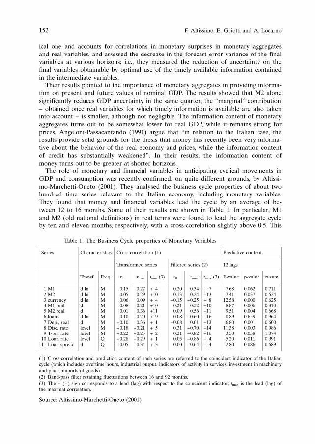
ical one and accounts for correlations in monetary surprises in monetary aggregatesand real variables, and assessed the decrease in the forecast error variance of the finalvariables at various horizons; i.e., they measured the reduction of uncertainty on thefinal variables obtainable by optimal use of the timely available information containedin the intermediate variables.Their results pointed to the importance of monetary aggregates in providing informa-
tion on present and future values of nominal GDP. The results showed that M2 alonesignificantly reduces GDP uncertainty in the same quarter; the “marginal” contribution– obtained once real variables for which timely information is available are also takeninto account – is smaller, although not negligible. The information content of monetaryaggregates turns out to be somewhat lower for real GDP, while it remains strong forprices. Angeloni-Passacantando (1991) argue that “in relation to the Italian case, theresults provide solid grounds for the thesis that money has recently been very informa-tive about the behavior of the real economy and prices, while the information contentof credit has substantially weakened”. In their results, the information content ofmoney turns out to be greater at shorter horizons.The role of monetary and financial variables in anticipating cyclical movements in
GDP and consumption was recently confirmed, on quite different grounds, by Altissi-mo-Marchetti-Oneto (2001). They analysed the business cycle properties of about twohundred time series relevant to the Italian economy, including monetary variables.They found that money and financial variables lead the cycle by an average of be-tween 12 to 16 months. Some of their results are shown in Table 1. In particular, M1and M2 (old national definitions) in real terms were found to lead the aggregate cycleby ten and eleven months, respectively, with a cross-correlation slightly above 0.5. This
152 F. Altissimo, E. Gaiotti and A. Locarno
Table 1. The Business Cycle properties of Monetary Variables
Series Characteristics Cross-correlation (1) Predictive content
Transformed series Filtered series (2) 12 lags
Transf. Freq. r0 rmax tmax (3) r0 rmax tmax (3) F-value p-value cusum
1 M12 M23 currency4 M1 real5 M2 real6 loans7 Dep., real8 Disc. rate9 T-bill rate10 Loan rate11 Loan spread
d lnd lnd lnddd lndlevellevelleveld
MMMMMMMMMQQ
0.150.050.060.080.010.10–0.10–0.18–0.22–0.28–0.05
0.270.290.090.210.36–0.200.36–0.21–0.25–0.29–0.34
+ 4+10+ 4+10+11+19+11+ 5+ 2+ 1+ 3
0.20–0.13–0.150.210.090.08–0.080.310.210.050.00
0.340.24–0.250.520.56–0.600.61–0.70–0.82–0.86–0.64
+ 7+13– 8+10+11+16+13+14+16+ 4+ 4
7.687.4112.588.879.510.896.8011.383.505.202.80
0.0620.0370.0000.0060.0040.6590.0010.0030.0580.0110.086
0.7110.6240.6250.8100.6680.9640.6000.9861.0740.9910.689
(1) Cross-correlation and prediction content of each series are referred to the coincident indicator of the Italiancycle (which includes overtime hours, industrial output, indicators of activity in services, investment in machineryand plant, imports of goods).(2) Band-pass filter retaining fluctuations between 16 and 92 months.(3) The + (–) sign corresponds to a lead (lag) with respect to the coincident indicator; tmax is the lead (lag) ofthe maximal correlation.
Source: Altissimo-Marchetti-Oneto (2001)

is roughly consistent with much of the international evidence available, particularlywith regard to M2.10 They also found a clear statistical link between nominal interestrates and the aggregate cycle. Interesting results were also obtained with the spreadbetween the interest rate charged on bank loans and that associated with medium andlong-term government bonds, which was found to be strongly countercyclical and tolead the aggregate cycle by four quarters, providing evidence in favour of the creditchannel of monetary transmission. In light of these features, they built a compositeleading indicator of the Italian cycle, including bank deposits in real terms and thespread between the interest rate on bank loans and the rate on long-term governmentbonds.
6. The use of the information in monetary aggregates in practice
The studies mentioned above represent the theoretical and empirical underpinning ofthe role attributed to monetary variables by the Bank of Italy. In practice, the use ofmonetary aggregates for day-to-day policy evaluation was based on the assessment oftheir deviations from a benchmark scenario and on the analysis of the factors underly-ing such deviations.A main forecasting exercise usually took place each year in the autumn and was
updated in the spring. It included the preparation of a ‘baseline’ forecast with thequarterly model and the selection of a number of alternative scenarios, with differentsets of policy and exogenous variables; a selected ‘normative’ scenario was then usedas an input for the monthly model to generate the monthly profiles for the main finan-cial aggregates, interest rates and monetary instruments. Monetary and financial fore-casts were then monitored during the year to detect deviations of the financial vari-ables from the projected paths and to interpret their implications for the overallpicture.The first announcement of the monetary growth path was made in October, and
stated in the October issue of the Bank of Italy’s Economic Bulletin. It was presentedconsistently with a simulation reproducing the (Government’s) macroeconomic planningscenario for the Italian economy and within a flow-of-funds framework, derived usingboth models. The projected paths for the main financial aggregates (credit to the non-state sector, total credit, total financial assets) complemented the announcement of themonetary growth objective (Table 2).The entire forecasting process played an important role in shaping the way the mone-
tary growth paths were announced to the public. Ex-ante, the caveats or qualificationsconcerning the underlying macro and financial framework, stemming from the forecast-ing exercise, were stressed, thus setting the stage for any ex-post discussion of possibledeviations of money from the announced path and of the appropriate policy response.In those cases where the money-income correlation was considered a reliable guide topolicy, and when it was intended to indicate that deviations from the reference path formoney would not be tolerated, the path was announced without qualifications. In 1990it was simply stated that “the target range for growth of the money supply has been setat 5–8 percent”;11 in 1992 it was stated that “the money supply growth target takes on
Monetary analysis in the Bank of Italy prior to EMU 153
10 See for example Kydland-Prescott (1990), Stock-Watson (1990), Cochrane (1994).11 See Economic Bulletin, October 1990, p. 58.

154 F. Altissimo, E. Gaiotti and A. Locarno
Table2.MonetaryTargetsandFlow-of-Funds
Gross
Domestic
Product
Totalcredit
tostate
sector(a)
Totalcredit
tonon-state
sector(b)
Totalcredit
ðaÞ+ðbÞ
Totalfinancialassests
Money(M2)
1000bln.
lire
%1000bln.
lire
%1000bln.
lire
%of
GDP
1000bln.
lire
%%of
GDP
1000bln.
lire
%%of
GDP
1000bln.
lire
%%of
GDP
1989
1990
1991
1992
1993
1994
1995(1)
1996(2)
1193.5
1312.1
1429.5
1504.0
1550.2
1641.1
1758.6
1872.6
9.3
9.9
8.9
5.2
3.1
5.9
7.2
6.5
125.5
148.7
138.9
81.1
22.3 7.8
51.2
72.0
20.1
20.0
15.9 8.2
2.0
0.7
4.3
5.8
132.7
139.6
151.2
164.1
161.5
158.8
133.0
112.4
11.1
10.6
10.6
10.9
10.4 9.7
7.6
6.0
258.2
288.3
290.0
245.2
183.8
166.6
184.2
184.4
15.8
15.2
13.4
10.0 6.7
5.6
5.9
5.6
21.6
22.0
20.3
16.3
11.9
10.2
10.5 9.8
202.7
221.7
244.7
180.0
147.7
182.3
174.2
177.1
13.7
12.8
12.8 8.3
6.2
7.1
6.3
6.0
141.7
146.1
152.0
157.3
164.9
168.4
167.1
166.4
62.7
79.1
74.3
41.6
75.5
17.4
16.0
55.0
8.6
10.7 8.5
5.9
8.2
1.9
1.2
5.0
61.6
62.1
62.2
61.8
64.9
62.3
59.1
58.4
Standardtablesettinggrowthrates(orranges)forM2togetherwithotherfinancialvariables.Thetablewasusuallypublishedin
theOctoberissueoftheEconomicBulletin.Annualflows,unlessotherwiseindicated.(1)Estimate(October).(2)Forecast.

greater importance for liquidity management and interest rate policy in the shortterm”12. In other cases, qualifications and uncertainties regarding the behavior ofmoney were stressed, as in 1995: “Assuming that the changes that have occurred in thecomposition of private financial portfolios this year do not continue, M2 should growby about 5 percent in 1996. However, the possibility that such shifts may continue . . .calls for particular caution in interpreting the behavior of monetary aggregates.”13
Sometimes, though not always, the implications of the monetary and financial frame-work for the interest rate policy were also spelled out. In 1996, it was made clear that“the growth in M2 . . . must be less than 5 percent in 1997. Assuming that the velocityof circulation . . . continues to increase at the rate observed in recent years, the pro-jected expansion in M2 is consistent with a reduction in interest rates”.14 Similarly, in1993 it was said that the monetary target “leaves room . . . for a reduction in the aver-age level of nominal interest rates”.15
While the macro forecast was usually made twice a year, the monthly analysis ofmonetary developments was used to put the forecast in perspective, assessing deviationsand detecting the sources of shocks hitting the economy.The monetary analysis transmitted to the Governor centered on, although it was not
limited to, the interpretation of the deviations of money growth from the projectedpath. Monthly deviations of money from the initial profile were monitored, using themonthly money demand equation as a starting point. Decomposition exercises, aimed atsingling out the economic determinants of deviations from the benchmark profile wereroutinely conducted. Econometric analysis, institutional information and anecdotal evi-dence were used to interpret the discrepancies. A standard decomposition exercise isshown in Table 3; the contribution of the right-hand-side variables in the money de-mand function to overall money growth are computed. The procedure could be basedeither on an analytical derivation or on a set of counterfactual simulations.16
In the case of instability in the equation, an analysis of institutional factors was con-ducted in order to distinguish pure financial disturbances from behavior that may re-flect some other sources of structural instability in the model. If the behavior of moneywas accounted for by changes in the explanatory variables, this was analyzed to checkwhether it was still consistent with the final targets.The weight assigned to money developments was not constant throughout the 1990s,
being influenced by the interpretation of its determinants. A number of examples ofhow different circumstances dictated different reactions to money growth can be foundin the internal briefing material.At the beginning of the 1990s, money demand showed remarkable stability and was
considered a reliable indicator. In the course of that year, in a context of rising infla-
Monetary analysis in the Bank of Italy prior to EMU 155
12 See Economic Bulletin, October 1992, p. 68.13 See Economic Bulletin, October 1995, p. 64.14 See Economic Bulletin, October 1996, p. 69.15 See Economic Bulletin, October 1993, p. 72.16 To estimate the contribution of a particular explanatory variable to money growth, a bench-
mark forecast is produced by keeping all explanatory variables in the money demand equationconstant at their value at the beginning of the simulation period (usually December); for eachvariable, a new forecast is then produced by inserting its actual behavior in the equation, whilekeeping the others fixed. The difference between the two forecasts gives the contribution of thevariable in question.

tionary pressures and expansionary fiscal policy, concern was expressed about strongerthan expected money growth. “Last September (1990), with M2 still growing at 7.4 per-cent, but with a higher profile for inflation, we forecasted annual growth of 10 percent(outside the reference range); we indicated the cause both in the more sustained pace ofprices and in the accumulation of high budget deficits in the following months. Our fore-casts did correctly anticipate the deviation of M2 from the target range, at a moment wereM2 was still in the centre of the range”.17 Consequently, monetary conditions were tigh-tened in October 1990, and justified to the public with the explicit aim of “curbing theexpansion of monetary aggregates” (Annual Report for the year 1990, p. 81).Later, soon after the exit of the lira from the exchange rate mechanism of the EMS,
the need for a clear nominal anchor was felt to be particularly pressing, and the beha-vior of money was watched carefully. However, in the course of 1993, deviations ofmoney growth from the announced profile were not considered a cause for concern,unlike in the previous example; they were traced to movements in the exogenous vari-ables that were not perceived as a threat to price stability. “The current trend suggeststhat, by the end of the year, M2 will be above the upper limit of 7 percent. The questionis whether the overshooting should be countered or whether, conversely, it should beannounced in advance and with what motivations. The announcement that limited devia-tions can be tolerated would be appropriate if it is judged that a change in monetarypolicy took place that is compatible with the inflation objective. This is likely to havehappened as an effect of the more pronounced cyclical slowdown, both domestic andinternational, and of the sharp decrease in interest rates in Europe. (This) . . . has createdthe conditions for a larger decrease in domestic rates, without worsening the risks of
156 F. Altissimo, E. Gaiotti and A. Locarno
Table 3. A Decomposition of M2 Growth(percentage change since the beginning of the year, s.a.)
Period Actualgrowth
Projectedgrowth
Contribution to projected growth
RealGDP
Prices Own rateon M2
T-billrate
Medium-term rate
T-bond ratevolatility
Laggedendo.at t0
1993. Dic 7.7 6.2 –0.35 4.13 –2.6 3.04 2.63 1.67 –2.56
1994. Jan 0.02 0.85 0.02 0.14 0.12 0.28 0.07 0.07 0.15
Feb 1.22 1.68 0.15 0.37 0.19 0.31 0.12 0.24 0.30
Mar 2.69 1.97 0.20 0.47 0.03 0.62 –0.05 0.45 0.25
Apr 3.28 2.21 0.33 0.86 –0.14 0.58 –0.06 0.64 –0.01
Mag 3.05 2.55 0.53 1.21 –0.09 0.43 –0.11 0.82 –0.25
In the model: yt ¼ ayt�1 þ b0xt þ "t ;
where xt is a vector of exogenous variables, the contribution of variable j to money growth over n months is:
bðjÞban�1xðjÞtþ1 þ an�2xðjÞtþ2 þ . . .þ xðjÞtþnc
Source: Unpublished note by G. Grande and R. Rinaldi, 28/6/1994.
17 Research Department note, 24/1/1991, referring to previous analyses in the second half of1990.
depreciation and imported inflation. Under these conditions, the anti-inflationary targetcould be compatible with a lower level of domestic rates and, temporarily, with morepronounced growth of the monetary aggregates”18. As a result of this analysis, the easingin monetary conditions was not interrupted. The analysis underlying the decision waslater presented to the market.19
The stability of the estimated money demand equations deteriorated in the last partof the decade, reflecting changes in the fiscal treatment of deposits and reserve require-ments, new structural trends in the portfolio choices of households, and possibly cur-rency substitution. As a consequence of these developments, the definition of M2 waschanged at the end of 1996, with the exclusion of some categories of CDs. In policyevaluation, greater attention was paid to the composition of money, together with itsaggregate behavior.20
In 1997 and 1998, in a context of declining interest rates and inflation rates,21 astrong increase in the growth of M2 was experienced, well above the announced value.In view of the observed instability of money demand, due to the above-mentionedfactors, this was not considered a sufficient reason to interrupt the decrease in interestrates. It was also observed that credit aggregates were growing at a very moderatepace, much less than forecast. However, money growth was still considered a sufficientreason to proceed with greater caution, given the highly uncertain outlook for inflation-ary expectations, the mixed signals coming from other indicators and the sustained in-crease in the most liquid components of money. “All in all, it is judged that these factors(the reform of the tax treatment of bank deposits, the structural changes in households’portfolios, the uncertainty of savers), which are to a large extent of a structural character,reduced the value of M2 in the current year as a leading indicator of inflationary pres-sures. The risks associated with an excessive growth in M2 appear, at present, to be lim-ited. However, these risks will have to be considered again should the growth of themonetary aggregate continue at the same pace observed in the first part of this year”.22
Again, the analysis was later presented to the public.23
All in all, in the 1990s the information value of money was more frequently affectedby episodes of money demand instability than in the preceding decade. The analytical
Monetary analysis in the Bank of Italy prior to EMU 157
18 Research Department note, 16/7/1993.19 “Analysis of the factors underlying the growth in M2 indicates that the relationship between
the monetary aggregate and its determinants has not been seriously undermined; the overshootingof the target can be explained mainly in terms of interest rate trends. . . . In view of the cyclicalslowdown in economic activity, which has been more pronounced than expected both in Italy andabroad, a reduction in interest rates and an expansion in M2 by more than forecast are compatiblewith attainment of inflation objectives” (Economic Bulletin, October 1993, p.71).20 In the second half of the 1990s monetary analysis was complemented by the use of Divisia mone-
tary indexes, mostly used as a cross-check of the behavior of simple-sum aggregates (Gaiotti, 1994).21 Previously, in 1994–95, the currency devaluation, the inflationary pressures and the worsening
of inflation expectations had been contrasted with a monetary tightening.22 Research Department note, 21/10/1997.23 ”In 1997 the growth in the M2 money supply was nearly twice the target of 5 percent, owing
chiefly to structural changes in the public’s portfolio preferences. This suggests that the value ofthe aggregate as an early indicator of inflationary pressures has been diminished, at least tempora-rily. Nevertheless, experience demonstrates that in the long run excessive monetary growth tendsto be reflected in price and exchange rate pressures. This consideration was one reason for thecaution with which monetary conditions were relaxed in the course of the year” (Annual Reportfor the Year 1997, pp. 123–124).
approach to assessing the information content in the context of the model of the Italianeconomy made it possible to treat money developments in a flexible way. More atten-tion was also paid, on particular occasions, to the liquid components of M2 (using,among other things, Divisia indexes) or to credit behavior. Reference to M2 growthremained an important anchor across the period, but was de-emphasized in some in-stances, particularly towards the end of the decade.
7. A test of the information value of monetary and credit aggregatesin the quarterly model of the Italian economy
Assessing the information value of money in the 1990s is interesting in the light of recentexperience. While several factors affected money demand in the past decade, the real sec-tor of the economy was also subject to important structural changes: among other things,the shift to the floating exchange rate regime in 1992–1996 and the reform in the wagebargaining system may have affected macroeconomic behavior and the process of expecta-tions formation in various ways. These changes may have also reduced the informationcontent of real variables, although the evidence on the existence of structural breaks isinconclusive.24 So, the issue of the marginal information content of money is left open.25
To assess the information content of monetary and credit aggregates in the 1990s, wechecked whether the most timely information on monetary and financial variables maybe used to improve the accuracy of forecasts of those variables of concern to the mone-tary authorities.The testing strategy we adopted, conceptually based on equation (2) above, is the
following: we computed the k-step-ahead (k = 1, 4, 8 quarters) forecast error of theendogenous variables of the quarterly model and checked whether surprises in mone-tary and credit variables were correlated with surprises in output and inflation. Thisapproach was suggested by B. Friedman to test for the marginal information value ofmonetary aggregates within a structural model, based on the consideration that “ifobserved money growth different from prior expectations also provides informationthat bears on future income growth”, then there is a role for money in guiding policy(Friedman (1984)).26 Detecting that surprises in monetary and real variables are statis-tically related justifies the role attributed to nominal aggregates in the conduct ofmonetary policy.
158 F. Altissimo, E. Gaiotti and A. Locarno
24 A discussion of the possible factors of instability in the quarterly model after 1992 is providedin Siviero-Terlizzese (1997). However, the evidence they present does not confirm the existence ofstructural breaks.25 The information content of money in a structural model has recently been questioned (Svens-
son-Woodford, 2000; Dotsey-Hornstein, 2000). By contrast, some results for the euro area, ob-tained with time-series methods, have stressed that money has some forecasting power for futureinflation (Nicoletti Altimari, 2000, Trecroci-Vega, 2000).26 The proposed approach has the advantage of being simple, but limitations and caveats must
clearly be emphasized. Goldfeld (1984) points out that the estimates may suffer from an omittedvariable bias, if some relevant information is not included in the equation (which should ideallyinclude the forecast errors for all the endogenous variables). This problem becomes more relevantfor longer forecast horizons, as the implicit assumption on the available information becomes moreand more questionable. For this reason, our experiment is limited to fixed and not too long fore-cast horizons, rather than concentrating on a dynamic simulation over the full sample, as Friedman(1984) did. In any case, the results must be considered contingent on the particular information setthat is assumed.

To implement this approach, we first ran simulations of the quarterly model over1989–2000, under the assumption of no uncertainty of exogenous variables, model coef-ficients and functional form specification.27
The quarterly model can be represented by the following set of equations:
yt �yTtyMtyOt
0B@
1CA¼ Fðyt;Yt�1;Xt;#Þ þ "t �
FTðyTt ; yMt ; yOt ;Yt�1;Xt;#ÞFMðyTt ; yMt ; yOt ;Yt�1;Xt;#ÞFOðyTt ; yMt ; yOt ;Yt�1;Xt;#Þ
0B@
1CAþ
"Tt"Mt"Ot
0B@
1CA (4)
where yt, the vector of modelled variables, is partitioned into three subsets, yTt ; yMt and
yOt corresponding to policy targets ðTÞ, monetary indicators ðMÞ and other endogenousvariables ðOÞ; "t is the vector of structural disturbances; Xt ¼ fxjgtj¼0 and Yt�1 ¼ fyjgt�1j¼0represent (present and) past history of the xs and ys and # is the vector of modelparameters. The n-period ahead forecast errors (surprises) are defined as:
yt � yt j t�n � ut j t�n ¼uTt j t�nuMt j t�n
uOt j t�n
0BB@
1CCA ¼ Fðyt;Yt�1;Xt;#Þ þ "t � Fðyt j t�n;Yt�1 j t�n;Xt;#Þ
(5)
where Yt�1jt�n ¼ fyj j t�ngt�1j¼0, with yt�j j t�n ¼ yt�j when j n. We set n to be equal to 1,4, 8 quarters. Then, for each horizon, we ran several variants of the following regres-sion, choosing the right-hand side variables in a parsimonious way:
uTt j t�n ¼ a þPpj¼l
bjuTt�j j t�n�j þ
Pqj¼k
gjuMt�j j t�n�j þ
Pqj¼k
djuOt�j j t�n�j þ ht ð6Þ
We chose surprises in real GDP and the GDP deflator as the left-hand side variablesðTÞ and M2, currency, credit to households, credit to firms and net domestic financialassets as financial indicators ðMÞ. The inclusion of the variable uOt j t�n, which representsa quickly available non-financial variable (in our case the index of consumer prices),allowed us to test whether the information content in monetary and credit aggregates isnot replicable by other sources. The values of the l, k, p and q parameters were chosenin such a way as to test whether surprises in financial indicators are related to surprisesin policy objectives; whether they contain additional information not contained in lagsof the endogenous variable; how this information changes as the information lag short-ens or lengthens and, finally, whether their forecasting power survives the introductionof non-financial indicators. We tested the statistical significance of monetary variables ineach equation allowing for heteroskedasticity and serial autocorrelation in the errorterm.Tables 4–5 report the main results for real GDP and the GDP deflator, respectively.
Each row refers to a regression of the n-period ahead forecast error of the final vari-able (defined as T in the tables) on the same forecast error for a monetary indicatorvariable, either contemporaneous or lagged (defined as M), as well the forecast errorfor the consumer price index (defined as O; this variable is included since the informa-
Monetary analysis in the Bank of Italy prior to EMU 159
27 The pre-EMU Italian definition of M2 was used, since most of the sample period lies beforethe start of Stage Three.
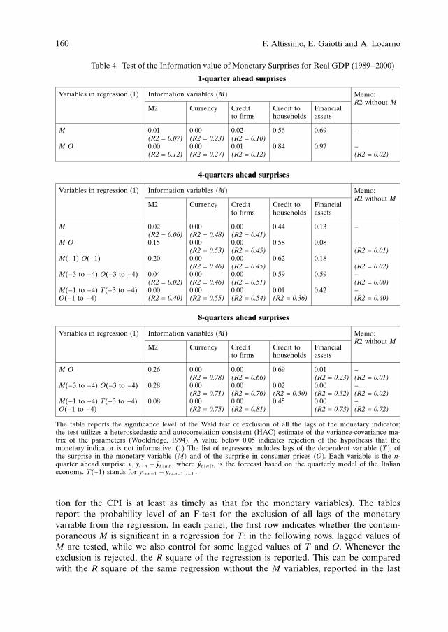
tion for the CPI is at least as timely as that for the monetary variables). The tablesreport the probability level of an F-test for the exclusion of all lags of the monetaryvariable from the regression. In each panel, the first row indicates whether the contem-poraneous M is significant in a regression for T; in the following rows, lagged values ofM are tested, while we also control for some lagged values of T and O. Whenever theexclusion is rejected, the R square of the regression is reported. This can be comparedwith the R square of the same regression without the M variables, reported in the last
160 F. Altissimo, E. Gaiotti and A. Locarno
Table 4. Test of the Information value of Monetary Surprises for Real GDP (1989–2000)
1-quarter ahead surprises
Variables in regression (1) Information variables ðMÞ
M2 Currency Creditto firms
Credit tohouseholds
Financialassets
Memo:R2 without M
M
M O
0.01(R2 = 0.07)0.00(R2 = 0.12)
0.00(R2 = 0.23)0.00(R2 = 0.27)
0.02(R2 = 0.10)0.01(R2 = 0.12)
0.56
0.84
0.69
0.97
–
–(R2 = 0.02)
4-quarters ahead surprises
Variables in regression (1) Information variables ðMÞ
M2 Currency Creditto firms
Credit tohouseholds
Financialassets
Memo:R2 without M
M
M O
M(–1) O(–1)
M(–3 to –4) O(–3 to –4)
M(–1 to –4) T(–3 to –4)O(–1 to –4)
0.02(R2 = 0.06)0.15
0.20
0.04(R2 = 0.02)0.00(R2 = 0.40)
0.00(R2 = 0.48)0.00(R2 = 0.53)0.00(R2 = 0.46)0.00(R2 = 0.46)0.00(R2 = 0.55)
0.00(R2 = 0.41)0.00(R2 = 0.45)0.00(R2 = 0.45)0.00(R2 = 0.51)0.00(R2 = 0.54)
0.44
0.58
0.62
0.59
0.01(R2 = 0.36)
0.13
0.08
0.18
0.59
0.42
–
–(R2 = 0.01)–(R2 = 0.02)–(R2 = 0.00)–(R2 = 0.40)
8-quarters ahead surprises
Variables in regression (1) Information variables (M)
M2 Currency Creditto firms
Credit tohouseholds
Financialassets
Memo:R2 without M
M O
M(–3 to –4) O(–3 to –4)
M(–1 to –4) T(–3 to –4)O(–1 to –4)
0.26
0.28
0.08
0.00(R2 = 0.78)0.00(R2 = 0.71)0.00(R2 = 0.75)
0.00(R2 = 0.66)0.00(R2 = 0.76)0.00(R2 = 0.81)
0.69
0.02(R2 = 0.30)0.45
0.01(R2 = 0.23)0.00(R2 = 0.32)0.00(R2 = 0.73)
–(R2 = 0.01)–(R2 = 0.02)–(R2 = 0.72)
The table reports the significance level of the Wald test of exclusion of all the lags of the monetary indicator;the test utilizes a heteroskedastic and autocorrelation consistent (HAC) estimate of the variance-covariance ma-trix of the parameters (Wooldridge, 1994). A value below 0.05 indicates rejection of the hypothesis that themonetary indicator is not informative. (1) The list of regressors includes lags of the dependent variable ðTÞ, ofthe surprise in the monetary variable ðMÞ and of the surprise in consumer prices ðOÞ. Each variable is the n-quarter ahead surprise x; ytþn � yytþnjt:, where yytþn j t: is the forecast based on the quarterly model of the Italianeconomy. T(–1) stands for ytþn�1 � ytþn�1 j t�1:.

column, to gauge the quantitative importance of the information variable. It should bestressed that the analysis is intended as a check of the explanatory power of monetarysurprises for the final variables, and it is not necessarily an accurate representation ofthe information set available to the policy-maker. In this respect, further analyseswould be warranted.As one would expect, the results are mixed. However, the empirical evidence
allows us to draw some general conclusions. First, the monetary indicators have in-
Monetary analysis in the Bank of Italy prior to EMU 161
Table 5. Test of the Information value of Monetary Surprises for the GDP Deflator(1989–2000)
1-quarter ahead surprises
Variables in regression (1) Information variables ðMÞ
M2 Currency Creditto firms
Credit tohouseholds
Financialassets
Memo:R2 without M
M
M O
0.70
0.86
0.20
0.23
0.00(R2 = 0.27)0.00(R2 = 0.34)
0.99
0.63
0.44
0.39
–
–(R2 = 0.04)
4-quarters ahead surprises
Variables in regression (1) Information variables ðMÞ
M2 Currency Creditto firms
Credit tohouseholds
Financialassets
Memo:R2 without M
M
M O
M(–1) O(–1)
M(–3 to –4) O(–3 to –4)
M(–1 to –4) T(–3 to –4)O(–1 to –4)
0.10
0.11
0.29
0.53
0.01(R2 = 0.44)
0.00(R2 = 0.32)0.00(R2 = 0.62)0.01(R2 = 0.47)0.00(R2 = 0.48)0.00(R2 = 0.76)
0.00(R2 = 0.53)0.00(R2 = 0.80)0.00(R2 = 0.80)0.01(R2 = 0.30)0.00(R2 = 0.74)
0.50
0.58
0.88
0.35
0.23
0.78
0.02(R2 = 0.30)0.02(R2 = 0.49)0.21
0.07
–
–(R2 = 0.41)–(R2 = 0.24)–(R2 = 0.01)–(R2 = 0.41)
8-quarters ahead surprises
Variables in regression (1) Information variables ðMÞ
M2 Currency Creditto firms
Credit tohouseholds
Financialassets
Memo:R2 without M
M O
M(–3 to –4) O(–3 to –4)
M(–1 to –4) T(–3 to –4)O(–1 to –4)
0.22
0.81
0.33
0.00(R2 = 0.93)0.00(R2 = 0.67)0.00(R2 = 0.84)
0.00(R2 = 0.95)0.00(R2 = 0.49)0.11
0.92
0.00(R2 = 0.60)0.00(R2 = 0.83)
0.00(R2 = 0.90)0.00(R2 = 0.34)0.00(R2 = 0.74)
–(R2 = 0.85)–(R2 = 0.19)–(R2 = 0.71)
The table reports the significance level of the Wald test of exclusion of all the lags of the monetary indicator;the test utilizes a heteroskedastic and autocorrelation consistent (HAC) estimate of the variance-covariance ma-trix of the parameters (Wooldridge, 1994). A value below 0.05 indicates rejection of the hypothesis that themonetary indicator is not informative. (1) The list of regressors includes lags of the dependent variable ðTÞ, ofthe surprise in the monetary variable ðMÞ and of the surprise in consumer prices ðOÞ. Each variable is the n-quarter ahead surprise x; ytþn � yytþn j t, where yytþn j t: is the forecast based on the quarterly model of the Italianeconomy. T(–1) stands for ytþn�1 � ytþn�1 j t�1:.
formation content, usually at all horizons. Second, it appears that the informationcontent of monetary aggregates is not limited to nominal magnitudes, but extends toreal ones as well. Third, currency and credit to firms outperform other monetaryand financial variables as leading indicators of future movements in output and in-flation.A more detailed examination of the empirical evidence suggests that, at short hori-
zons, surprises in M2 are not a significant explanatory variable for the GDP deflator.Contemporaneous surprises in M2 have some information content for real GDP, butthe share of explained variance of the surprise (as measured by the corrected Rsquare) is extremely low. Moreover, the exclusion of M2 surprises for GDP is oftenaccepted when lags of the left-hand side variable are included in the regression. Theseresults are consistent with the anecdotal evidence, suggesting that M2 had a limitedinformation content in the 1990s; they are also consistent with the cautious approachadopted by the Bank of Italy in the second half of the decade in responding to move-ments in M2.However, other monetary indicators seem to have information content. Surprises in
currency significantly enter both the equations of the GDP deflator and real GDP, andthey remain significant when lags of the dependent variable are included. In most caseswhere currency surprises enter the equation significantly, the increase in the R squareof the equation is between 0.3 and 0.5. This result, too, is consistent with the approachadopted by the Bank of Italy towards the end of the decade, which paid somewhatgreater attention to the behavior of the more liquid components of M2; the latter wereprobably less affected by the fiscal and regulatory changes that took place in thoseyears. It should be noted that during the period under consideration the growth ofcurrency was also highly correlated with the growth of overnight deposits; this suggeststhat M1 could be a promising candidate as an information variable in our exercise.Unfortunately, a demand equation for M1 was not readily available for the whole peri-od and the test could not be performed.The results also suggest that credit to firms may have an informative role. This marks
a difference with the evidence and the conventional wisdom in the 1980s. Surprises tocredit to firms usually enter significantly the equations for both the GDP deflator andreal GDP, over all horizons. Credit to households less frequently enters the regressionsin a significant way. The result is not unexpected; the share of households’ indebtnessin Italy is much lower than all others OECD countries, and recourse to debt financingby households is limited (although it has been increasing in recent years).
8. Conclusions
We draw the following conclusions from both the descriptive and the econometric evi-dence discussed above.The Italian experience confirms that money can have information content and be an
important guide to policy, even in a model where it is demand-determined. Thus, thefoundations for the role of money do not need to involve a choice between models of‘active’ vs. ‘passive’ money.However, deciding what weight to attach to monetary variables in guiding short- and
medium-term policy-making is essentially an empirical matter. The Italian experiencesuggests that the information content of M2, which was found to be large in the 1980s,
162 F. Altissimo, E. Gaiotti and A. Locarno
was smaller in the 1990s, when a series of structural changes affected the stability ofmoney demand. Indeed, the weight assigned to M2 in different episodes has changed;however, the whole set of monetary indicators still played an important role. The con-ceptual framework used to interpret the information contribution of monetary vari-ables, based on the structural model of the Italian economy, was explained in advanceto the public. The policy reaction to monetary developments could be justified, depend-ing on the interpretation of the observed instability in money demand, on the behaviorof the explanatory variables in the money demand equation and on their consistencywith the overall macroeconomic framework.In this respect, the Italian experience suggests that an essential feature of the pol-
icy framework is to grant flexibility to the policy-maker, e.g. to allow the possibilityof adjusting the weight assigned to money according to particular circumstances, butto do so without losing consistency and credibility. When facing deviations of somevariables from the forecast path, the use of the structural models of the Italian econ-omy made it possible to tell a consistent ‘story’, in which an interpretation of theobserved behavior of various variables was provided and a policy interpretation pre-sented. The reference to a consistent conceptual framework, in which the role of thevarious indicators could be cross-checked and evaluated, was an essential componentof the strategy.
References
Altissimo, F., D. J. Marchetti and G. P. Oneto (2001), “The Italian Business Cycle: Coincident andLeading Indicators and Some Stylized Facts”, Giornale degli Economisti e Annali di Economia,Vol. 60.
Angelini, P., D. Hendry and R. Rinaldi (1994), “An Econometric Analyisis of Money Demand inItaly”, Banca d’Italia, Temi di discussione, No. 219.
Angeloni, I. (1994), “The Bank of Italy Monthly Money Market Model. Structure and Applica-tions”, Economic modelling, Vol. 11, No. 4, pp. 387–412.
Angeloni, I. and A. Cividini (1990), “Il valore informativo delle variabili finanziarie: un’analisi conil modello econometrico della Banca d’Italia”, Banca d’Italia, Temi di discussione, No. 134.
Angeloni, I. and F. Passacantando (1991), “Monetary policy in Italy. Institutional and EconomicAspects”, in Bank for International Settlements, The orientation of monetary policy and themonetary policy decision-making process, Basle, April.
Bank of Italy, Economic Bulletin, various issues.Bank of Italy, Abridged Report, various issues.Bank of Italy (1986), “Modello trimestrale dell’economia italiana”, Banca d’Italia, Temi di discus-
sione, No. 80.Bank of Italy (1988), “Modello mensile del mercato monetario “, Banca d’Italia, Temi di discus-
sione, No. 108.Bank of Italy (1989), Abridged Report for the Year 1988. Governor’s concluding remarks.Bank of Italy (1995), Abridged Report for the Year 1994. Governor’s concluding remarks.Bank of Italy (1996), Abridged Report for the Year 1995. Governor’s concluding remarks.Bank of Italy (1997), Abridged Report for the Year 1996. Governor’s concluding remarks.Ciampi, C. A. (1987), “Italy’s Changing Financial Markets: Implications for Monetary and CreditPolicy”, in Bank of Italy, Economic Bulletin, February.
Cochrane, J.H. (1994), “Shocks”, Carnegie-Rochester Series on Public Policy, Vol. 41, pp. 295–364.Dotsey, M. and A. Hornstein (2000), “Is The Behavior of Money Useful to a Discretionary Policy-maker?”, manuscript, Federal Reserve Bank of Richmond.
Friedman, B. M. (1984), “The Value of Intermediate Targets in Implementing Monetary Policy”, inPrice Stability and Public Policy, edited by the Federal Reserve Bank of Kansas City, KansasCity.
Monetary analysis in the Bank of Italy prior to EMU 163

Friedman, B. M. (1990), “Targets and Instruments of Monetary Policy”, in B. M. Friedman and F.H. Hahn , Handbook of Monetary Economics, North-Holland.
Gaiotti, E. (1992), “L’evoluzione dei metodi di controllo monetario e il modello mensile della Ban-ca d’Italia”, manuscript, Banca d’Italia.
Gaiotti, E. (1994), “Measuring Money with a Divisia Index: an Application to Italy”, Banca d’Ita-lia, Temi di Discussione, No. 223.
Gaiotti, E., A. Gavosto and G. Grande (1998), “The Rise and Fall of Inflation in Italy in the1990s: a Comparative Analysis of Four Different Explanations”, Giornale degli Economisti eAnnali di Economia, Vol. 57, No. 3–4, pp. 297–324.
Gaiotti, E. and S. Nicoletti Altimari (1996), “Monetary Policy Transmission, the Exchange Rateand Long-Term Yields under Different Hypotheses on Expectations”, Banca d’Italia, Temi didiscussione, n. 276.
Galli, G., D. Terlizzese and I. Visco, “Short and Long Run Properties of the Bank of Italy Quar-terly Econometric Model”, Dynamic Modelling and Control of National Economy, Vol. 2, IFACsymposium, Edinburgh, 27–29 June.
Goldfeld, S. M. (1984), Commentary on B. Friedman, in Price Stability and Public Policy, edited bythe Federal Reserve Bank of Kansas City, Kansas City.
Gressani, D., L. Guiso and I. Visco (1988), “Disinflation in Italy: an analysis with the QuartelyModel of the Bank of Italy”, Journal of Policy Modeling.
Kydland, F. and C. Prescott, (1990), “Business Cycles: Real Facts and a Monetary Myth”, FederalReserve Bank of Minneapolis Quarterly Review, Spring, pp. 3–18.
Nicoletti Altimari, S. (2000), “Does money lead inflation in the euro area?”, ECB Working PaperNo. 63.
Nicoletti Altimari, S., R. Rinaldi, S. Siviero and D. Terlizzese (1995), “Monetary Policy and theTransmission Channels in the Bank of Italy’s Quarterly Econometric Model” in BIS, FinancialStructure and the Monetary Policy Transmission Mechanisms.
Siviero, S. and D. Terlizzese (1997), “Crisi di cambio e innovazioni nei comportamenti: alla ricercadi discontinuita strutturali nel modello econometrico della Banca d’Italia” in Banca d’Italia,Ricerche quantitative per la politica economica.
Siviero, S., D. Terlizzese and I. Visco (1999), “Are Model-Based Inflation Forecasts Used in Mone-tary Policymaking? A Case Study”, Banca d’Italia, Temi di discussione, No. 357.
Stock, J. and M. Watson, (1990), “Business Cycle Properties of the Coincident Economic Indica-tors”, in Lahiri and Moore (eds.), Leading Economic Indicators, Cambridge.
Svensson, L. and M. Woodford (2000), “Indicator Variables for Optimal Policy”, manuscript.Trecroci, C. and J. L. Vega (2000), “The Information Content of M3 for Future Inflation”, Euro-pean Central Bank, Working Paper No. 33.
Wooldridge, Jeffrey, M. (1994) “Estimation and Inference for Dependent Processes”, in Engle, R.and D. L. McFadden (eds.), Handbook of Econometrics, vol. IV.
164 F. Altissimo, E. Gaiotti and A. Locarno
“In its coverage of economic conditions in the Federal Republic of Germany the Bundes-bank has always given special attention to the money supply. In its ‘Monetary Analyses’it has regularly investigated how the stock of money has changed and what factors havebrought about the changes.” (Deutsche Bundesbank, Monthly Report July 1971, p. 11)
1. Introduction
The insight that inflation is, in the long run, a monetary phenomenon was already dee-ply anchored in the perception of the general public in Germany long before the policyof monetary targeting was introduced. This conviction was visibly reflected in the Bun-desbank Act of 1957, which expressly committed the Bundesbank to regulating thecurrency in circulation and the supply of credit to the economy in order to safeguardthe currency. Accordingly, the observation and analysis of developments in the mone-tary aggregates as well as their components and counterparts has a similarly long tradi-tion in Germany. Bearing that in mind, it is also understandable that the Bundesbankturned to this natural stability anchor when it first announced a monetary target inDecember 1974 following the final collapse of the Bretton Woods system and the at-tainment of far-reaching freedoms in taking monetary policy action. Up to the time offoregoing autonomy in monetary policy with the start of European Monetary Union,the money stock continued to occupy the top position in the hierarchy of indicatorswithin the Bundesbank’s monetary policy (Konig, 1996, p. 125). Analysing and com-menting on monetary developments on the basis of the consolidated balance sheet ofthe banking system was of prominent importance both in preparing decisions internallyand for explaining monetary policy decisions that had been taken.This paper has the following structure: Chapter 2 gives a brief account of the essen-
tial elements of the Bundesbank’s monetary targeting strategy. Chapter 3 is concernedwith the basic elements and general principles of the Bundesbank’s analysis of the con-solidated balance sheet of the banking sector. Following this, in the Chapters 4 to 9periods in which the analysis of the consolidated balance sheet was of particular impor-tance for the interpretation of monetary developments are discussed. Finally, Chapter10 summarises the most important findings.
The role of the analysis of the consolidated balance sheetof the banking sector in the context of the Bundesbank’smonetary targeting strategy prior to Stage Three
Julian Reischle
Deutsche Bundesbank*
* The views expressed in the paper are those of the author and not necessarily those of theBundesbank. Thanks for helpful comments made by Peter Schmid and Gaby Kabelac as well as bymy discussants Sandrine Scheller and Patrick Lunnemann of the Banque Centrale du Luxembourgand by the participants of the ECB conference.

2. Basic features of the Bundesbank’s monetary targeting strategy
The Bundesbank had always attributed a special role to the money stock within itsintermediate-target-oriented strategy.1 For that reason, the Bundesbank announced amonetary target for the first time in 1975 (see the annex for a table of the Bundes-bank’s monetary targets). Proceeding from a medium-term orientation, the Bundesbankderived the stability-oriented rate of monetary expansion from the aggregate key vari-ables for potential growth, the unavoidable rate of price increases (later, “normativeinflation rate” or the “medium-term price assumption”) and the trend rate of change inthe velocity of circulation. Starting with the target formulated for 1979, the Bundesbankswitched from a single-figure target for average annual monetary growth to setting atarget path with a target corridor for monetary expansion during the year (between thefourth quarter of the previous year and the fourth quarter of the current year). An-nouncing a target for the money growth in the course of the year had the major advan-tage of showing the importance of controlling the monetary expansion continuously.The formulation of a target corridor not only helped to take account of the sometimesquite sharp short-term random fluctuations in the money stock – in the first half of theeighties it was also used deliberately by the Bundesbank as an instrument for makingmonetary targeting more flexible. The – in some cases – clear failures to meet thetarget in the first four years of its monetary policy strategy had taught the Bundesbankthat single-figure targets were too ambitious precisely in the light of “unforeseeableexternal disturbances . . . – such as oil price shocks or sharp monetary policy changes,affecting interest rates, in other countries with which Germany has close ties – . . .”(Deutsche Bundesbank, 1980, p. 30). By contrast, a corridor with a specification of theconditions for an orientation more to the top or bottom edge of the corridor or with aregular review of the monetary target at mid-year enabled the Bundesbank to counterunexpected risks to price stability more easily.2 The use of four-quarter targets ratherthan target averages had the additional advantage that the Bundesbank was able tomake adjustments for failure to meet the previous year’s target or for very sharp orweak monetary expansion at the end of the previous year (a monetary overhang) de-spite the comparatively invariant key macroeconomic variables in the derivation of thetarget.Initially, the Bundesbank formulated its monetary target for the “central bank money
stock” as defined by the Deutsche Bundesbank. In addition to currency in circulation –less cash balances of the domestic credit institutions –, this definition contained thebanks’ required minimum reserves on domestic liabilities at constant reserve ratios asat January 1974. Minimum reserves were to be held on sight deposits as well as theholding of time and savings deposits with a maturity or period of notice of less than
166 Julian Reischle
1 On the Bundesbank’s monetary policy strategy, see, for example, Issing (1992), Deutsche Bun-desbank (1995a), Konig (1996), Neumann (1997), Schmid (1998).
2 In each of the years from 1979 to 1983, the Bundesbank announced which edge of the corri-dor monetary expansion should incline to. Accordingly, in the years of monetary policy tightening(1979 to 1981) the bottom half of the corridor was targeted and, in the years of economic down-turn (1982 and 1983) the top half. Thereafter, no such specifications were made. Instead, greaterattention was devoted to reviewing the corridor regularly in mid-year. However, only once (1991)did such a review result in an adjustment being made. This consisted in a lowering of the wholecorridor by 1 percentage point.
four years.3 Precisely the weighting of the various bank deposits, which was intended toreflect their varying liquidity, was highlighted as a crucial advantage compared withunweighted, broadly defined aggregates. Even so, the central bank money stock wasclosely related to these aggregates, since it represented “the reflection of non-banks’(weighted) money balances in the Bundesbank’s Weekly Return” (Deutsche Bundes-bank, 1985, p. 14/15). Not least, however, the central bank money stock was, at thesame time, also supposed to express the Bundesbank’s responsibility for the rise inmoney balances. After all, without any action by the Bundesbank the banks’ balancesat the central bank were unable to rise (Deutsche Bundesbank, 1985, p. 15).With its monetary target for 1988 the Bundesbank switched to basing its monetary
target directly on the broadly defined aggregate M3 – consisting of currency in circula-tion excluding the credit institutions’ cash balances and the sight deposits, time depositsfor less than four years and savings deposits at three months’ notice held by domesticnon-banks at domestic banks. Even though the deposits that were subject to minimumreserve requirements were very largely the same ones that also formed part of themoney stock M3, and both aggregates had therefore developed over time mostly inparallel, the different weighting of the components did result in marked differences inthe recorded pace of growth in individual periods (see Figure 1).4 The divergent devel-opments had invariably been due to a perceptible reaction of currency in circulation toextreme fluctuations in interest and exchange rates. Owing to the higher weighting ofcurrency in the central bank money stock, these fluctuations had a much greater impacton this aggregate than on M3. Owing to the fear at the end of 1987 that disturbingfactors would lead to a persistent distortion in the demand for currency, a decision wasmade to change the key operational variable.5
Despite its intermediate-target-oriented monetary policy strategy, at no time did theBundesbank use the money stock as a “monetary autopilot”; shorter-term deviations ofmonetary expansion from the target path, viewed in isolation, never led to a purelymechanistic response on the part of the central bank. What was crucial for the role ofthe money stock in taking interest-rate decisions was always its informative value forfuture price developments; after all, the monetary target was merely an intermediateobjective on the road to safeguarding price stability. The comparatively narrow gearingof monetary policy to a monetary aggregate over the years was thus only made possible
The role of the analysis of the consolidated balance sheet of the banking sector 167
3 Specifically, this was 16.6% for sight deposits, 12.4% for time deposits and 8.1% for savingsdeposits. From March 1978, the credit institutions had been allowed to deduct their monthly aver-age cash holdings at least up to an amount equal to 50% of their required reserves (Section 7.3 ofthe Bundesbank’s Minimum Reserves Order as amended on March 1, 1978). Since the incentive torestrict cash balances to an absolutely necessary minimum now no longer appeared to apply, theBundesbank feared that such cash balances would increase sharply overall and also become morevolatile. With a view to the potential negative implications for the monetary intermediate targetvariable, from March 1978 the deductible cash balances were no longer included when determiningthe central bank money stock (Deutsche Bundesbank, Monthly Report, June 1978, p. 18/19).
4 One difference between the two aggregates was that the central bank money stock includedthe minimum reserves on savings deposits of over three months’ notice but less than four yearsand savings bonds with a maturity of less than four years – all of which were not part of themoney stock M3.
5 Given the large number of financial innovations in many industrial countries, the Bundesbankperceived an additional advantage of M3 in its unweighted construction allowing new forms ofinvestment to be incorporated more easily than by the central bank money stock (Deutsche Bun-desbank, 1988b, p. 20).
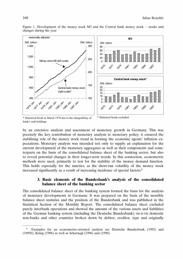
by an extensive analysis and assessment of monetary growth in Germany. This wasprecisely the key contribution of monetary analysis to monetary policy; it ensured thestabilising role of the money stock trend in forming the economic agents’ inflation ex-pectations. Monetary analysis was intended not only to supply an explanation for thecurrent development of the monetary aggregates as well as their components and coun-terparts on the basis of the consolidated balance sheet of the banking sector, but alsoto reveal potential changes in their longer-term trends. In this connection, econometricmethods were used, primarily to test for the stability of the money demand function.This holds especially for the nineties, as the short-run volatility of the money stockincreased significantly as a result of increasing incidence of special factors.6
3. Basic elements of the Bundesbank’s analysis of the consolidatedbalance sheet of the banking sector
The consolidated balance sheet of the banking system formed the basis for the analysisof monetary developments in Germany. It was prepared on the basis of the monthlybalance sheet statistics and the position of the Bundesbank and was published in theStatistical Section of the Monthly Report. The consolidated balance sheet excludedpurely interbank operations and showed the amount of the various assets and liabilitiesof the German banking system (including the Deutsche Bundesbank) vis-a-vis domesticnon-banks and other countries broken down by debtor, creditor, type and originally
168 Julian Reischle
���
���
���
�����
�����
�����
��
� �
��
� �
���
� �
����
� �
����
� �
���
� �
���
� �
���
��
���
��
���
��� ������� ��� �������
�� ��� ��� �������
����� ����� �� ��!� �� ��"
#���$ � � �� %���� �����
$�&'� �� ��"(
� ���������� ��� �� ����� ���� ��� �� ��� ����������� ��
�� �� ���� ��������
��
�
��
��
��
��
��
��
���
����
����
���
���
��� �������
������ ���� ���� ������
�
���
���
��
��
���
����
����
���
���
��� �������
� ���������� ��� ��������
Figure 1. Development of the money stock M3 and the Central bank money stock – stocks andchanges during the year
6 Examples for an econometric-oriented analysis are Deutsche Bundesbank (1992) and(1995b), Konig (1996) as well as Scharnagl (1996) and (1998).
agreed maturity. Principally, reports by the banks were used for this purpose. Thesereports had to be prepared by the banks in accordance with the provisions of the Bank-ing Act on prudential grounds.7 Although general reporting requirements had alreadybeen introduced for all banks when the Bank deutscher Lander had been established in1948, a reporting obligation was not enforced initially for all credit institutions, mainlyfor technical reasons. In particular, smaller credit cooperatives were not recorded in themonthly balance sheet statistics to begin with. From December 1985, however, the Bun-desbank did switch to a complete survey. A wave of mergers in the cooperative bank-ing sector had meant in any case that a large number of exempted institutions hadsince been incorporated into credit cooperatives that formed part of the reporting po-pulation.8
For the purposes of monetary analysis, the consolidated balance sheet of the bankingsystem was prepared as a table (text table in the Monthly Report “Money stock and itsdeterminants” and, later, “The money stock and its counterparts”). This overview tableshowed the monthly changes – adjusted for purely statistical effects – that had takenplace in bank lending to domestic non-banks, the net external assets of the bankingsystem, domestic non-banks’ monetary capital formation at domestic banks, other fac-tors and the Federal Government’s deposits in the domestic banking system.9 The bot-tom line showed the monthly increase or decrease in the money stock.In the sixties and even in the early seventies, the Bundesbank initially derived the
balance of the change in bank lending to domestic non-banks and monetary capitalformation. This balance was interpreted as an “internal money creation balance”. De-ducting the change in the (longer-term) liabilities of German credit institutions to do-mestic non-banks not counted towards the money stock, the balance was intended toindicate the contribution made by the domestic source of money creation – in otherwords, bank lending – to the creation of the money stock. With the Bretton Woodscrises it became apparent, however, that monetary capital formation was being fed notonly by the domestic expansion of credit but also – and mainly – by heavy inflows offunds from abroad. The internal money creation balance lost its value as an informa-tion variable for monetary policy and balancing was no longer appropriate.It later proved to be more appropriate, in fact, to combine lending to domestic non-
banks and the change in the net external position in one variable for the “overall avail-able domestic capital and credit sources” (Deutsche Bundesbank, 1987, p. 42) or the“banks’ assets-side business” (Deutsche Bundesbank, 1996, p. 62). This took account ofthe observation that, from the point of view of domestic borrowers, borrowing fromdomestic or foreign banks was generally closely substitutable for each other. Looking
The role of the analysis of the consolidated balance sheet of the banking sector 169
7 Linking the balance sheet statistics to the banks’ prudential reports to the Bundesbank islikely to have enhanced the correctness of the reports submitted (Schlesinger, 1984, p. 5).
8 The reporting requirement was initially geared to the balance sheet total of the credit coop-eratives. Starting from Reichsmark 2 million (balance sheet date March 31, 1948) or DM 500,000(from January 1955; relevant balance sheet date 31 Dec. 1953) this limit was raised in severalstages to DM 10 million. Until the overall survey was instituted in December 1985 all credit coop-eratives were required to report, whose balance sheet total on 31 Dec. 1972 amounted to DM 10million or more or which were already subject to reporting requirements on 30 Nov. 1973.
9 Until the balances of the central and regional authorities were freed from the deposit require-ment at the Bundesbank as of January 1, 1994 owing to the entry into force of the second stage ofEuropean Economic and Monetary Union, this item corresponded to the central bank deposits ofthe domestic public sector.
solely at credit expansion, as a guiding principle for the trend of monetary expansion,would have produced a false picture of the underlying driving force for monetary ex-pansion. It was decided not to combine them in this way in the table, however, in ordernot to devalue the importance of lending and external transactions for monetary capitalformation.The definition of the money stock – the level of which was shown in the consoli-
dated balance sheet and the development of which was primarily intended to provideinformation on the monetary situation in Germany – did not remain unchanged overthe years. Generally, there was a tendency on the part of the Bundesbank to extend theoriginally very narrow definition of the money stock more and more as time went on.As early as the mid-sixties, besides the “classical” monetary aggregate M1 – consistingof currency in circulation (excluding the cash balances of the credit institutions) and thesight deposits of domestic non-banks – a money stock aggregate was being calculatedwhich additionally included time deposits – initially with a period of notice of sixmonths and, from 1968, for three months.10 This aggregate, which was now named M1a,was replaced at the start of the seventies by a more broadly defined money stock con-cept: the money stock M2. Besides M1, this included “quasi-money”, in other words,time deposits for less than four years.11 The money stock M1 was now (only) one partof the “money stock in the broader sense” (M2). Savings deposits at three months’notice had initially been deliberately excluded from being considered for defining themoney stock, since their low transactions velocity had meant that they had been as-cribed more the character of a “long-term accumulation of capital” (Deutsche Bundes-bank, 1971, p. 13). From the middle of 1975 onwards, however, they were indeed usedfor calculating the money stock M3 – the “money stock in the broadest sense”. Tobegin with, there were only verbal references to the trends in this broadly defined ag-gregate and a mention as a memorandum item in the Monthly Report table “Themoney stock and its counterparts”, but in mid-1976 M3 finally attained the prominentimportance in the analysis of the consolidated balance sheet of the banking sector thatit retained up to the end.12 This was in no way changed by the money stock “M3 ex-tended”, which was introduced to the general public for the first time in the 1986 An-nual Report and which was commented on regularly from the start of 1990. In additionto the components of M3, M3 extended comprised the bank deposits of domestic non-banks with the foreign subsidiaries and foreign branches of German banks (Euro-de-posits), and the short-term bank bonds issued by German banks (with a maturity of upto two years) and – from August 1994 onwards – the certificates of money marketfunds held by domestic non-banks (less the bank deposits and short-term bank bondsheld by domestic money market funds).The Bundesbank’s preference for more broadly defined monetary aggregates – in
which it included the central bank money stock as defined by the Bundesbank in addi-
170 Julian Reischle
10 This slight narrowing in the time deposits had become possible as a result of a new maturitybreakdown which had been introduced in the balance sheet statistics at the end of 1968. This madeit possible to focus even more strongly on “cash holdings affecting payments” without totally ne-glecting the frictions in the synchronisation of the payment flows.
11 The first reference to this aggregate was in the Monthly Report of July 1971, pp. 11–13.12 The first systematic listing of the three aggregates M1, M2 and M3 was in the Monthly Re-
port of June 1976, p. 11. From July 1976, M3 appeared “below the line” in the table showingmonetary growth.
tion to M3 – was explained by the high interest-rate sensitivity of the narrow aggre-gates (for example, in Deutsche Bundesbank, 1985, p. 18–21.). The money stock M1, inparticular, reacted strongly to the cyclical movements of the short-term interest rates.Interest-rate increases, for instance, quite quickly triggered shifts into higher-yieldingforms of investment, especially into shorter-term time deposits. Even though the M1holdings had fallen, the investors had not become perceptibly less liquid; there hadbeen scarcely any change in the liquidity situation in the economy. For the Bundes-bank, M1 therefore represented more of a measure for the monetary policy stimulusthan for the stock of money influencing demand in the economy. As a consequence ofextensive portfolio shifts, M1 understated monetary expansion. Similarly, albeit in theopposite direction, the aggregate M2 was also affected by interest-rate-induced shifts. Inperiods of sharply rising short-term interest rates, it were mainly time deposits for up tofour years which benefited since both sight deposits and shorter-term savings depositswere shifted into them. M2 thus tended to develop in the opposite direction to theinterest rate policy. It was therefore not least owing to its comparatively steady devel-opment that the Bundesbank selected the money stock M3 as its key point of referencefor the monetary analysis and later as its intermediate target aggregate. The observa-tion of more narrowly defined aggregates (such as M1 or M2), components and coun-terparts was only undertaken in order to better assess the development of M3. Thecomparatively low statistical explanation power argued against M3 extended.An additional disadvantage of the money stock M3 extended – but also of the cen-
tral bank money stock – was the fact that one could not see the reason behind itsexpansion. In contrast, M3 had the advantage of being an integral element of the con-solidated balance sheet. Although one has to be careful when making statements aboutcausal relationships on the basis of the consolidated balance sheet, it gave some hintsabout possible reasons. By including the Euro-market deposits and, later, the moneymarket fund shares, the money stock M3 extended obviously went beyond the consoli-dated balance sheet, since additional statistical information was needed to form it. Inaddition to the monthly reports of the foreign subsidiaries and branches of Germanbanks, which made it possible to determine the amount of Euro-market deposits, thecapital market statistics had to be used to calculate the money market fund shares incirculation. Even the key monetary policy reference variable from 1975 to 1987, thecentral bank money stock as defined by the Deutsche Bundesbank, could not be takendirectly from the consolidated balance sheet, but had to be derived instead from thereturn of the central bank and the minimum reserve statistics. The data of the monthlybalance sheet statistics were also supplemented by various additional surveys. In thiscontext, besides quite detailed quarterly borrowers statistics and lending commitmentsstatistics, mention should be made, above all, of the external position of the credit insti-tutions, which broke down the bank’s external assets and liabilities by country and cur-rency. Furthermore, yet other statistics were used for interpreting monetary trends, in-terest-rate statistics and balance of payments statistics being only two examples.
4. Periods of particular challenges for the analysis of the consolidatedbalance sheet of the banking sector – an overview
Given the sometimes considerable short-term random fluctuations in monetary growth,ultimately only the analysis of the consolidated balance sheet of the banking sector wasable to impart a certain degree of sureness to the assessment of current monetary de-
The role of the analysis of the consolidated balance sheet of the banking sector 171
velopments. Especially in periods when the money stock deviated from its target path,there had to be an answer to the question of whether this divergence was merely ran-dom in nature or whether it was perhaps indicative of a longer-term trend. Puttingmonetary developments in the context of the prevailing interest-rate and income situa-tion – as the essential factors influencing private sector money holdings – a search wasmade for (other) reasons for the short-term growth of the money stock both in thecomponents and their counterparts. It can, in actual fact, be observed that in the peri-ods when either various monetary indicators were showing a mixed picture or when themonetary aggregates were revealing particularly striking behaviour, there was either avery flat or even an inverse yield curve or that serious institutional changes (tax law,minimum reserve regulations, change in the provisions governing savings, authorisationof new forms of investment) and external changes (exchange rate) had occurred.13 Afew periods are cited below as examples of times in which the analysis of the consoli-dated balance sheet was of particular importance for assessing monetary growth. Eventhough periods are assigned to particular “special developments”, this does not imply thatthe identified factor was the sole cause of the monetary expansion in question. Given thelarge number of individual money holders and a continuously changing monetary policysetting, monetary growth invariably reflects a whole range of different factors.14
5. Monetary policy in times of a sharp appreciation in the D-Mark –1986 and 1987
Although monetary expansion in 1985 had been consistent with the target, the pace ofmoney stock growth had started to pick up as early as the start of 1986, and acceler-ated even more sharply in the middle of the year and persisted throughout 1987. Theoriginally envisaged growth of the central bank money stock between the fourth quar-ter of the previous year and the fourth quarter of the current year of 3 I% to 5% for1986 and 3% to 6% for 1987 was clearly exceeded at 8% in both 1986 and 1987 (seeFigure 2). The impression of an excessively sharp rise in money holdings was also con-firmed by the expansion of the other aggregates, especially the money stock M3. Aboveall, in 1986 the quite similar growth rates in the various money stock definitions sug-gested that the increase in the central bank money stock was being underpinned bothby an excessive increase in currency in circulation and by the minimum reserve compo-nent – and thus by all its underlying bank deposits. By contrast, the distorting indicatorproperty of the central bank money stock known to the Bundesbank again becomeapparent in 1987, which was caused by the high weighting of currency.15 The low oppor-tunity costs of liquidity holdings due to low short-term interest rates as well as quite asharp rise in the amounts of currency held abroad had bloated currency in circulation
172 Julian Reischle
13 For similar breakdowns of such factors, see, for example, Konig (1996, p. 118–121), who,however, ascribes the effects on the term structure to disruptions in the capital market (see alsoSchmid, 1998, p. 14).
14 For a more chronological analysis of monetary developments in Germany between 1975 and1995, see for example Kole and Meade (1995, p. 922–927).
15 During 1986, the monetary aggregate M3 increased, at 7 J%, approximately as sharply asthe central bank money stock (7 %). In 1987, however, the increase was significantly lower(6 I%) than in the case of the central bank money stock (8%). The assessment that there was asharp monetary expansion was nevertheless confirmed both times in principle.

exceptionally in 1987. The expansion of the money stock M3 during the year, at 6 I%,was therefore also less sharp in that year.16
To a considerable extent, the sharp appreciation in the D-Mark in those two yearshad contributed to a sharp increase in cash holdings – presumably mostly outside Ger-many. Despite an increase in the surplus on current account, appreciation expectationsfor the D-Mark as well as marked speculation on interest rates had resulted in a highnet import of capital (see Figure 3).17 There were extensive inflows of funds fromabroad to domestic non-banks, leading to a rise in the net external asset position of thebanking system.18
As is usual in such periods, the large inflows of funds from abroad in 1986 and 1987had not only led to a sharp rise in money holdings but had simultaneously curbedbanks’ lending to domestic non-banks. Obviously, there was a close substitutional linkbetween borrowing from domestic credit institutions and borrowing abroad. Precisely insuch a situation, it proved to be helpful for assessing monetary developments to com-bine domestic lending and the change in the net external position. A “domestic finan-cing potential” determined in this way expanded comparatively sharply in both 1986
The role of the analysis of the consolidated balance sheet of the banking sector 173
���
���
���
���
���
���
�
����
��
���
��
�
����
��
���
��
�
����
��
���
��
�
��� �������
���� �����
� � �! " � � �!
���� �����
�! " �!
���� �����
�! " �!
� ���������� ��� �� ����� ���� ��� �� ��� ����������� ��
�� �� ���� �������#
��
�
�
�
�
��
���
��
����
��
����
��
���
��
����
��
���
���
����
����
����
����
���
���
����
����
����
��� ��������� ��� �������������� �� ����� ����� � ���!"
�#��$��� %���� �� �&� '�(�$) �$�*&� � ���!""
'(� +������
� �������������� � ��� ���� ������ ������� � ���
����������� ������� ����� �� �������
�� ����� ��������� ! ���� �� "�#��� �������� ����
������ �$ ���%����� ��%�����
Figure 2. Development of the Central bankmoney stock 1985–1987
Figure 3. Net inflow of external funds and de-velopment of the external value of the D-Mark
16 Average of the fourth quarter of 1987 compared with the average of the fourth quarter of1986.
17 Short-term, low-interest funds taken up in the Euro-market were used for financing Germanbonds (Deutsche Bundesbank, 1986, p. 38).
18 Rohde (1996, p. 62ff.) identifies a clear connection between D-Mark appreciation and mone-tary growth for other periods as well. Masuch (1994) likewise provides an analysis of the externalinfluences on German monetary policy.
and 1987; the banks’ entire asset-side business had thus perceptibly fostered monetarygrowth. Another factor was a low propensity on the part of investors to invest over themedium term; given the low interest rate of such investments and in the expectation ofinterest rates rising again, domestic non-banks adopted a “wait-and-see” attitude.For 1986 and 1987, therefore, the analysis of the consolidated balance sheet of the
banking sector discerned a high rate of monetary growth. Additionally incorporatingthe deposits of domestic non-banks at the foreign subsidiaries and branches of Germanbanks – the Euro-market deposits – in the analysis of the monetary aggregates showedan expansion in 1986 that was even higher than already indicated by M3.19 The factthat the Bundesbank nevertheless lowered central bank interest rates in 1986 and 1987,rather than raising them, was mainly justified by the sharp appreciation in the D-Markagainst the US dollar (Deutsche Bundesbank, 1986, p. 34–36 and Deutsche Bundes-bank, 1987, pp. 38–40). An interest-rate increase would probably have given furtherencouragement to the appreciation tendencies of the D-Mark and thus additionally in-tensified the economic impact of the trend in the exchange rate. Given the fact thatappreciation had made imports cheaper and the dramatic fall in oil prices, the risks toprice stability were, if anything, rated as slight. The overshootings of the monetary tar-gets therefore appeared to be acceptable on the whole. After all, the monetary targetswere not an end in themselves but were intended solely to help safeguard price stabi-lity. The overshootings of the target in 1978 and 1979 were justified in a similar man-ner. These likewise occurred in times of a sharp D-Mark appreciation, although ex-change-rate developments were not their primary cause.
6. Monetary policy in the wake of the ERM crisis 1992/93
A growth of the money stock that was very sharp to begin with in the summer monthsof 1992 – in August 1992, M3 already exceeded its average of the fourth quarter of1991 at a seasonally adjusted annual rate of some 8 I% – was joined in autumn 1992by disruptions in the wake of the turbulence within the ERM. This turbulence initiallyled to a further acceleration of monetary expansion because the inflows largely bene-fited domestic non-banks. This was reflected by a rise in the banks’ net external assetposition. The Bundesbank’s foreign exchange inflows amounting to DM 82 I billionwas accompanied by an increase in the banking system’s net external position of asmuch as DM 42 I billion. This meant that the inflow of funds to domestic non-bankswas more than twice as high as in the months particularly affected by the D-Markappreciation speculation in the mid-eighties taken together.20 Besides non-residents’ ac-quisition of German bonds, this was probably due to German enterprises high debt inforeign currency abroad. Added to this might have been an increased holding of D-Mark balances by multinational companies. In this period of expectations of a sharpappreciation in the D-Mark, an early redemption of liabilities denominated in D-Mark
174 Julian Reischle
19 The money stock “M3 extended” which, in addition to M3, also comprised the (in 1986sharply risen) Euro-deposits and the (perceptibly falling) bank bonds with a maturity up to oneyear (from 1990 with a maturity of up to two years) in the hands of domestic non-banks rose justas sharply, at 7%, as the central bank money stock.
20 Specifically, this had mainly been the months December 1985 to March 1986 and January toFebruary 1987. In the months April and Mai 1986 as well as March 1987, high external outflowsoccurred in each case as a counter-reaction (Deutsche Bundesbank, 1993b, p. 28).

by foreign debtors as well as German importers delaying foreign-currency payments foras long as possible might have also been factors contributing to the sizeable inflows offunds to the domestic non-banks.Even though the heavy inflows of funds to non-banks had perceptibly dampened
both short-term borrowing by private non-banks and lending to the public sector inSeptember 1992, the money stock M3 rose in that month at a seasonally adjusted an-nual rate of 27%. This increase particularly affected sight and time deposits. Thesewere evidently being used to “park” short-term inflows of funds. After the wave ofspeculation had receded and the reversal of external payments flows, there followed acorrective movement in the money stock, but the rate of monetary expansion neverthe-less remained quite high for some time. This confirmed the earlier empirical findingthat in periods of high appreciation expectations, a bloating of liquidity occurs morequickly than a subsequent return to normal.During the tensions in the ERM in summer 1993 the formula “speculation on D-Mark
appreciation equals a sharp increase in the rate of monetary expansion” did not hold.Despite an intervention volume of DM 60 billion in July 1993, there was, in fact, a fall inthe net external position of the banking system in that month. The funds thus flowedpredominantly to German banks and not to domestic non-banks; the interventions thusremained more or less neutral in terms of their impact on the money stock. Similarly,the expectation of a D-Mark appreciation at the end of the seventies played only aminor role in the excessive monetary expansion of that period. It was precisely the perse unclear role played by external influences in the increase in the money stock whichtaught the Bundesbank that it had to identify the causes of monetary growth at all timeswith the aid of the analysis of the consolidated balance sheet of the banking sector.
7. Monetary policy in periods when there was an inverse term structure– the “liquidity jam” in 1992 to 1994 and in 1996
Besides externally induced distortions, shifts between money stock components andmonetary capital have always exerted a strong influence on the rate of monetary expan-sion. Such shifts were mostly a reaction to existing interest-rate differentials betweenshort and long-term investments of funds, with tax motives being an added factor (seeFigure 4). Probably mainly on account of an inverse term structure – in other words,short-term assets being remunerated at a higher rate than long-term ones – as well asuncertainty about future interest-rate movements, a pronounced “wait-and-see” attitudeconcerning monetary capital formation set in from 1992 up to early 1994. Funds whichhad previously been invested over the longer term became free and were “parked” inliquid accounts. Although the Bundesbank had been steadily lowering short-term inter-est rates since autumn 1992, by the end of 1993 it had not managed to effect a crucialreduction in the interest-rate advantage of shorter-term investments. This was due to thefact that, not least owing to external influences, German capital market rates, too, werefollowing the downward trend they had been on since the end of 1990. Since the moneystock M3 had increased sharply in 1992 and 1993 owing to other “special factors” in anycase, the existing interest-rate advantage of shorter-term assets and the unclear directionin which longer-term interest rates were heading led to a further bloating of M3. Over-all, the Bundesbank was forced to recognise that the “surge in liquidity” had run into aconsiderable “liquidity jam” (Deutsche Bundesbank, 1994b, p. 21).
The role of the analysis of the consolidated balance sheet of the banking sector 175

Notwithstanding the failures to meet the monetary targets in 1992 and 1993, as wellas the still-accelerating monetary expansion at the beginning of 1994, the Bundesbankresponded in spring 1994 by a lowering of interest rates by a cumulative total of 1 Jpercentage points. The aim of this was “to encourage the acquisition of longer-termfinancial assets by increasing the interest rate gap between short and long-term assets,and thus to contribute to dampening monetary growth and the associated fears of infla-tion” (Deutsche Bundesbank, 1994a, p. 68). In addition to this interest-rate-policy mea-sure, the interest-rate rise in the capital market was probably the main factor that alsoplayed a crucial part in freeing up the liquidity jam in the financial markets from mid-1994 onwards (Issing, 1996, p. 121).This interest-rate policy of the Bundesbank, which runs exactly counter to the tradi-
tional concept of the reaction of the money stock to changes in the short-term interestrate, could ultimately only be justified by the special factors prevailing at the end of1993 and at the start of 1994. The indispensable role of analysis of the consolidatedbalance sheet of the banking sector in this lay in determining the underlying causes of
176 Julian Reischle
��
�
�
�
�
�
��
����
��
�
����
��
�
����
��
�
����
��
�
����
��
�
���
��
�
����
��
�
����
��
�
����
��
�
����
��
�
����
��
�
����������� ����
������ �� ����� ���������� !
"������� ���� ��##��������
�
�
�
�
�
��
��
����
��
�
����
��
�
����
��
�
����
��
�
����
��
�
���
��
�
����
��
�
����
��
�
����
��
�
����
��
�
����
��
�
$
$������% &�'���� #��������
� ����� ���� �� ������� ��� �� ��� � ���������� �� ������ ��������� �� �� ��� �� ���������� �� �����������
Figure 4. Interest-rate development and shifts between the money stock M3 and the monetary capitalformation (12-month growth rates, in%)

monetary expansion and thus in identifying the prevailing special factors.21 The trans-mission mechanisms of monetary policy to the money stock are just not always time-invariant, as is frequently assumed. This insight and the interest-rate decisions derivedfrom it did not imply any departure by the Bundesbank from its monetary targetingstrategy. The Bundesbank found support for its adherence to the monetary targetingstrategy in the internal and external econometric studies which were largely unable tofind empirical evidence of an unstable long-run money demand equation in Germany(see for example Deutsche Bundesbank 1995b, p. 31–37).In spring 1996, the Bundesbank found itself facing a similar situation. At that time, too,
monetary capital formation was very weak owing to special factors. Instead, M3 wasclearly above the target corridor, since savings deposits with a period of notice of threemonths, in particular, were rising sharply. The additionally formed savings deposits weremainly special savings facilities, however, which did formally have a three-month period ofnotice, but which yielded much higher rates of interest than the traditional savings depositsat three months’ notice if there was a contractual agreement to forgo notice.22 To thatextent, they were a substitute for the long-term forms of savings traditionally counted to-wards monetary capital (savings deposits with an agreed period of notice of over threemonths or time deposits with an agreed maturity of four years or more). The fact that, in1996, long-term savings deposits were greatly reduced, while the holding of savings bondsremained unchanged, indicates that a part of monetary capital formation was recorded defacto in M3 and that M3 was therefore overstated.23 In turn, an added factor was uncer-tainty about interest-rate developments in the capital market, which resulted in a “wait-and-see” attitude in the case of monetary capital formation. Uncertainty played an impor-tant role in the following years, too. Especially in 1998 “the historically low capital marketrates, the flattened yield curve, and the occasionally quite pronounced uncertainties infinancial markets” (Deutsche Bundesbank, 1998, p. 82) dampened the propensity to accu-mulate longer-term financial assets with the banking sector. On the basis of a more med-ium-term orientation to the average expansion of M3 as well as comparatively low growthin the money stock M3 extended and the banks’ largely unchanged assets-side business,the Bundesbank arrived at an overall assessment that the provision with liquidity was gen-erous but by no means excessive. In this case, too, the Bundesbank – superficially counterthe signals given by the money stock – decided to lower interest rates.
8. Monetary policy in times of institutional change –the authorisation of money market funds in mid-1994
Following the extremely sharp growth in the money stock M3 at the end of 1993, whichpersisted in the first quarter of 1994 – M3 had risen in seasonally adjusted terms by16% on the quarter – a corrective movement in the monetary trend set in towards the
The role of the analysis of the consolidated balance sheet of the banking sector 177
21 The unconventional interest-rate measure did, of course, encounter objections; this also con-cerned the credibility of the monetary targeting strategy (for critical appraisals, see, for example,Goldman and Sachs, 1994, p. 5ff. or Rohde, 1996, p. 231ff.).
22 With the entry into force of a new provision governing savings in mid-1993, the credit insti-tutions increasingly switched to offering more attractive forms of savings. Throughout the nineties,the higher-yielding special forms of savings were the cause of the renaissance in Germany of sav-ings deposits at three months’ notice.
23 In principle, this portfolio-shifts continued until summer 1999. It is only since autumn 1999that not only the traditional savings deposits at three months’ notice but also the higher-yieldingspecial forms of savings have been run down.

middle of the year. This movement became even stronger towards the end of 1994 andeven led to an absolute seasonally adjusted decline in the money stock M3 at the turnof 1994/95. One important factor that contributed to this development was domesticnon-banks’ large-scale acquisition of money market fund certificates that do not counttowards the money stock M3 (see Figure 5). In July 1994, the Central Bank Council ofthe Deutsche Bundesbank had set aside its previous reservations against D-Markmoney market funds, which now made it possible for units in such funds to be issued inGermany, too. Domestic and foreign funds made very active use of this opportunity; upto the end of the year, domestic non-banks acquired certificates to the amount of DM46 billion, of which just under DM 27 billion was accounted for by the month of De-cember alone. This “enthusiasm” for what was a new form of investment in Germanywas encouraged not only by their attractive remuneration combined with comparativelyhigh liquidity, but also by their preferential wealth-tax treatment.24 The latter factorexplains their great popularity at the end of the year.Among the counterparts of the money stock M3, the acquisition of money market
fund certificates was reflected, above all, by quite high outflows in foreign payments -which had a dampening impact. To the acquisition of foreign money market fund certi-ficates was added a fairly pronounced involvement by domestic funds in the Euro-mar-ket (Deutsche Bundesbank, 1994a, p. 82). The large-scale withdrawal of non-residentsfrom the DM bond market had also been no less of a cause for the sharp drop in thenet external asset position in 1994, however.However, the analysis of the consolidated balance sheet of the banking sector
showed that it would be too simplistic to explain the collapse in the development of M3in the second half of 1994 exclusively in terms of the acquisition of money market fundcertificates by domestic non-banks and the outflows of funds to non-residents which
178 Julian Reischle
���
�
��
��
��
��
����
�
�
���
�
�
�
�
����
�
�
�
�
� � �������
Figure 5. Purchases/sales of domestic and foreign money market funds shares by German non-banks
24 In contrast to other (directly held) financial assets, only half the rate had to be paid for fundcertificates in connection with capital taxation (Deutsche Bundesbank, 1994a, p. 78).
this generated. It was rather the case that monetary growth was also curbed by theperceptible surge in monetary capital formation in mid-1994. Above all, funds “parked”in short-term time deposit accounts were shifted into monetary capital on a large scale.Besides longer-term bank bonds, time deposits with a maturity of four years or morebenefited from this shift. The overall quite sharp expansion of lending to domestic non-banks was thus faced with an additional dampening influence in addition to outflows inforeign payments.Another reason for not overemphasising the influence of money market fund certifi-
cates on German monetary growth is that, while the money stock M3 initially contin-ued to grow only very weakly in 1995, domestic and foreign money market fund certifi-cates were purchased only to the equivalent of just under DM 7 billion. The dampeningimpact in 1995 was thus very slight. Since, in the two following years, money marketfund certificates of just under DM 20 billion were resold, their introduction had not onthe whole led to a permanent distortion of the pace of monetary growth. Even thoughthe abrupt increase in this form of investment had clearly disturbed monetary growth atthe turn of 1994/95, the Bundesbank saw no reason for departing from its monetarytargeting strategy.
9. Monetary policy in times of institutional change –the influence of tax legislation on monetary developments
It is unlikely that there are any influencing factors which impaired of M3’s function asan indicator of underlying monetary trends as often as tax legislation. Besides varia-tions in the taxation of interest income on forms of monetary investment, the introduc-tion and expiration of tax incentives for investment also deserve mention here – theyhave impacted on monetary growth by either inflating or deflating lending by banks.The following list must therefore be limited to important changes.
9.1. Changes in taxes on interest income
� Even in the run-up to the introduction of the 10% tax on all domestic interest in-come which was introduced on January 1, 1989, massive evasive reactions occurred.At the end of 1988 “an increase in currency in circulation which was completely outof line” (Deutsche Bundesbank, 1988a, p. 39) took place, with domestic investorsvirtually fleeing to cash.25 Instead of long-term investment of funds with domesticbanks (monetary capital formation), not only was cash squirreled away, but therewere also shifts in sight deposits and Euro-market deposits. However, the strongestincrease was in holdings of foreign securities. Even the mere announcement of theintroduction of taxation on interest income starting at the beginning of 1989 wasenough to cause major shifts of monetary asset formation from Germany abroad in1988. In the face of public pressure, the Federal Government felt compelled, as earlyas in May 1989, to abolish capital gains taxes on interest income effective July 1. Formonetary developments, this “tax policy experiment” had the inglorious effect ofcausing the money stock, having already missed the target in 1986 and 1987, to
The role of the analysis of the consolidated balance sheet of the banking sector 179
25 In December 1988 currency in circulation rose at a seasonally adjusted rate of 46 I%. Bycontrast, the increase in December 1999, as the millennium was coming to a close, was, at 23%,only half as high.

clearly overshoot the upper limit of the target corridor in the fourth quarter of 1988as well. Outflows in cross-border payments were not a real counterweight to themeagre formation of monetary capital and the rather large growth of lending in thelight of low interest rates. Moreover, it caused investors to rediscover the virtues ofthe Euro-market; Euro-deposits were replenished very strongly in the years that fol-lowed thanks to their attractive interest rates (see Figure 6). At least part of thosefunds probably represented “a. . . shifting of domestic cash balances to the reserve-exempt ‘offshore centres’ of the Euro-market” (Deutsche Bundesbank, 1989, p. 39),meaning that their rise went along with an impairment of M3’s indicator function –even if it was only temporary in nature. The consequence was a closer observation ofM3 extended in monetary analysis, however, without doing away with M3 as theprominent indicator.
� At the beginning of 1993 a new attempt was made to tax domestic interest income.Effective January 1, 1993, a tax on interest income of 30% was introduced. Now, too,the end of the previous year saw extensive hoarding of cash and major shifts of fundsabroad. Cash stockpiling even turned out to be greater than at the end of 1988.26 Yetas before, the impact on the willingness of domestic investors to deposit long-termfunds with German banks is likely to have been a more important factor in the devel-opment of M3. As a consequence of the inverse yield structure, monetary capitalformation was exceptionally weak both in the second half of 1992 and in the first fewmonths of 1993. In addition to shifts in shorter-term bank deposits with domesticcredit institutions, a share of the funds envisaged for deposit was placed with foreignbanks – especially in Luxembourg. Also, the purchase of foreign investment fundshares by domestic non-banks was particularly high. Via foreign investment compa-nies, a large share of the funds shifted abroad returned to the German capital mar-
180 Julian Reischle
26 In December 1992 alone, cash in circulation rose at a seasonally adjusted annual rate of61 I%.
���
� � � �
� � � � �
�����
�����
�����
�����
� �
� �
� �
� �
� �
� � �
� � �
� � �
� � �
� � �
� � �
� � �
� � �
� � �
� � �
� � �
��� ������
� � �
� � �
Figure 6. Short-run deposits of German non-banks at foreign branches and foreign subsidiaries ofGerman banks
ket, however. Bank debt securities also benefited, meaning that the dampening im-pact on monetary capital formation, both in 1992 and 1993, was in actual fact likelyto have been less pronounced than indicated by the statistics. Therefore, monetarycapital formation tended to be understated.27
� As a reaction to the shift of monetary capital formation to Luxembourg, starting onJanuary 1, 1994 the tax on interest income was extended to include foreign growthinvestment funds. At the end of 1993, therefore, there was a repatriation of fundsheld abroad which distinctly exceeded the window-dressing which German investorsalways did at the end of the year. As a consequence of the unclear direction of long-term interest rates, the funds were first parked on the already very healthy short-term time deposit accounts. Additionally, sight deposits and shorter-term savings de-posits benefited as well – the latter also due to an institutional change. Also, in viewof the growth rates of the money stocks M1, M2 and M3, which all shot past thereference corridor for M3 growth, the Bundesbank gained the impression that thedomestic non-banks’ liquidity situation at the end of 1993/beginning of 1994 wasrather abundant. Looking back at the preceding months, the Bank noted that“money holdings . . . shifted temporarily between Germany and abroad . . . constitutea considerable potential source of disruption of domestic monetary growth”(Deutsche Bundesbank, 1993a, p. 69).
9.2. Changes in tax incentives for borrowing
In the wake of German unification, many tax incentives for investing in eastern Ger-many were introduced. This bloated the demand for credit and distorted the role of theinterest rate as an operating variable. Scaling back those programmes or already exist-ing programmes or allowing them to expire, especially programmes granting tax creditsfor private homebuilding, in some cases caused grave anticipatory effects in domesticlending: the distortion of lending to domestic non-banks mostly seeped through all theway to monetary growth. In addition, the role of credit aggregates as an indicator ofthe long-run effects of monetary policy was distorted. Credit aggregates have neverbeen particularly important as an indicator for price developments in Germany, anyway.In nearly all years following 1993, tax-related reasons can be found for the continuouslyhigh rise in medium to long-term loans and advances of domestic non-banks. The taxmeasures introduced at the beginning of 1993/94 and 1997 had a particularly distinctimpact.
� The measures to limit write-off possibilities for the purchase of owner-occupied oldbuildings adopted in May 1993 as part of a “Federal consolidation programme”, partof which were to take effect on January 1, 1994, led to a wave of premature housingpurchases and a sharp rise in homebuilding loans. In December 1993 alone, mediumto long-term loans and advances to private non-banks rose by a seasonally adjusted19%, with roughly half of those loans being attributable to homebuilding purposes.
The role of the analysis of the consolidated balance sheet of the banking sector 181
27 In its overview of monetary developments in terms of the balance sheet (based on adjustedchanges), in the past the Bundesbank adjusted the German bank debt bonds in issue for those soldto non-residents or purchased from non-residents. Since the statistical inaccuracies of the underly-ing balance-of-payment data were well-known, these corrections were not explicitly taken into ac-count in the levels listed in the consolidated balance sheet.
Over all of 1993 the rise in medium to long-term lending was 11%; this made itdistinctly higher than could be reconciled with the weak growth of the German econ-omy. The expansionary impact on the money stock linked to the heavy lending, to-gether with the above-mentioned return flows of foreign funds and the low propen-sity to deposit funds over the longer term, led to a strong bloating of M3, whichpersisted beyond the end of 1993, held firm until mid-1994 and then was adjustedinto 1995. Since the “Federal consolidation programme” also envisaged a further re-duction in tax promotion of owner-occupied old buildings starting on January 1, 1995,borrowing throughout 1994, too, was marked by anticipatory effects in the purchasingof residential property. Two-thirds of all new medium to long-term loans taken up bydomestic non-banks were attributable to homebuilding purposes. Private-sector bor-rowing, motivated not least out of tax considerations, was, in an overall view, themost important source of the high monetary growth in 1994. Along with comprehen-sive outflows of funds in payments to non-residents, only the monetary capital forma-tion which kicked in in mid-year posed a true counterweight and made it possible forthe money stock M3 to swerve into the target corridor at the end of the year.
� In 1996, too, housing loans expanded particularly strongly compared with other lend-ing to the domestic private sector. Besides a change in tax promotion of owner-occu-pied housing which took effect at the beginning of that year, the reduction in specialdepreciation facilities for new rental housing in eastern Germany starting on January1, 1997 probably had a major impact. The simultaneous raising of the tax on theacquisition of land and buildings probably unleashed additional anticipatory effects.Besides medium- to long-term housing loans, as the end of the year 1996 approached,short-term lending was likewise perceptibly replenished before being turned intolonger-term loans over the course of the following year. Since in 1996 the propensityto form (domestic and foreign) monetary capital was relatively low due to low long-term interest rates, the tax-policy-related distortions in lending for housing purposesled, on the whole, to monetary growth that overshot the target corridor.
10. Conclusions
In summary, it may be noted that the analysis of the consolidated balance sheet of thebanking sector has been an indispensable element in assessing the monetary dynamicsin Germany. Only this was able to give the Bundesbank’s M3-oriented monetary policythe necessary security, for only with its help could disturbances in the indicator qualityof the money stock be identified in a relatively short time. Especially in the nineties,the M3 monetary aggregate was repeatedly exposed to disturbances. Although this wasreflected in a stronger short-term volatility of the money stock M3, it did not disruptthe underlying long-term relationship between M3 and price movements in Germany.Thus, monetary analysis – and therefore the analysis of the consolidated balance sheet– has formed the basis for a policy of “pragmatic monetarism” (Schmid 1998, p. 20)and “rule-based discretion” (Neumann 1997, p. 196). Looking back on the years be-tween 1975 and 1998, the following conclusions may be drawn:
� The consolidated balance sheet of the banking system formed the basis for this analy-sis. The money stock M3 ascertained on that basis has, over large stretches of time,been the key orientation variable for judging monetary developments. Even when
182 Julian Reischle
the central bank money stock as defined by the Deutsche Bundesbank representedthe intermediate target, M3 growth was analysed and commented upon in an on-going manner. It often served to ensure the accuracy of signals being emanated bythe central bank money stock. Wherever extreme reactions in cash holding exerciseda dominant influence on the central bank money stock, changes in the central bankmoney stock were mostly put into perspective with a reference to M3 growth.
� Even after the transition to the M3 intermediate aggregate, the Bundesbank did notstop at observing and commenting upon M3 growth. Much as the dynamics of thecentral bank money stock were often juxtaposed with the growth of M3, M3 growthwas later compared especially with growth of M3 extended. Such an approach madeit possible to assess monetary growth more reliably. However, M3 stayed in the mid-point of the analysis and at the top of the indicator hierarchy. However, if the aggre-gates under observation sent different signals, the reasons were always explained indepth if the M3 aggregate was not followed.
� This was mostly achieved by analysing the components and counterparts of M3. Thisanalysis always took place in view of the components’ and counterparts’ significanceto M3 growth. The Bundesbank has never left any doubt that lending aggregateshave, in its view, never been indicator variables equivalent to the money stock M3.True, lending growth has had an impact on monetary growth; however, lending aggre-gates, because they develop broadly in parallel to price rises, have no inherent infor-mative value in respect of the future rise in prices.
� Although the long-term connection between the money stock and prices in Germanyhas been rather stable over the years, the shorter-term volatility of M3 rose sharplyin the nineties. One particular reason for this was the existence of numerous disrup-tive factors which either had an unusually dampening impact on monetary capitalformation or distorted lending. Strong changes in exchange rates also played a role,as did changes in tax law or the authorisation of money market funds.
� For interest rate decisions, short-term developments of the monetary aggregate werenever relevant. Rather, its trend was important. If the monetary expansion was dueto strong growth of bank lending, which tends to reflect the long-run effects of mone-tary policy, interest rate hikes were appropriate. However, if the cause was a pro-nounced “wait-and-see” attitude in monetary capital formation, a reduction in theinterest rate could help increase the propensity to invest over the longer term. In theevent of a strong monetary expansion thanks to appreciation-related capital inflows,it was generally advisable to first wait and see so as not to provoke further capitalshifts by raising interest rates. Here, one could hope that domestic price movementswould not pick up due to the cheapening of imports despite a sharp rise in themoney stock.28
� On the whole, monetary targeting is likely to have helped in the establishment of asolid monetary policy reputation. Particularly the certain degree of “hands-tying” andthe associated obligation to explain and justify deviations of the money stock fromthe target path have been helpful here.
The role of the analysis of the consolidated balance sheet of the banking sector 183
28 This variety of reactions by monetary policy to the development of the money stock is likelyto have contributed to the money stock not having any significant impact in most estimates of theBundesbank’s reaction function (e.g. in Bernanke and Mihov (1997), Clarida and Gertler (1996) orBerger and Woitek (1996)); Schachter provides an overview of such studies and her own results(1999, pp. 257–311.).

Appendix
References
Berger, Helge and Ulrich Woitek (1998), Economics or Politics: What Drives the Bundesbank?,Munchner Wirtschaftswissenschaftliche Beitrage.
Bernanke, Ben S. and Ilian Mihov (1997), What Does the Bundesbank Target? In: European Eco-nomic Review, Vol. 41, pp. 1025–1053.
Clarida, Richard and Mark Gertler (1996), How the Bundesbank Conducts Monetary Policy,NBER Working paper, No. 5581.
Deutsche Bundesbank (1971), Longer Term Movements of the Money Stock, in: Monthly Reportof the Deutsche Bundesbank, July 1971, pp. 11–27.
Deutsche Bundesbank (1980), Annual Report 1980.Deutsche Bundesbank (1985), The Longer Term Trend and Control of the Money Stock, in:
Monthly Report of the Deutsche Bundesbank, January 1985, pp. 13–26.
184 Julian Reischle
Monetary targets and their implementation
in %
Target:growth of the central bank Actual growthmoney stock or the money stock M3 1 (rounded figures)
in the as an more precisecourse of annual definition during in the course as an annual Target
Year the year 2 average the year of the year 2 average achieved
1975 8 – – 10 – no1976 – 8 – – 9 no1977 – 8 – – 9 no1978 – 8 – – 11 no1979 6–9 – Lower limit 6 – yes1980 5–8 – Lower limit 5 – yes1981 4–7 – Lower half 4 – yes1982 4–7 – Upper half 6 – yes1983 4–7 – Upper half 7 – yes1984 4–6 – – 5 – yes1985 3–5 – – 5 – yes1986 3 1=2 –5
1=2 – – 8 – no1987 3–6 – – 8 – no1988 3–6 – – 7 – no1989 about 5 – – 5 – yes1990 4–6 – – 6 – yes1991 3 3–5 – – 5 – yes1992 3 1=2 –5
1=2 – – 9 – no1993 4 1=2 –6
1=2 – – 7 – no1994 4–6 – – 6 – yes1995 4–6 – – 2 – no1996 4–7 – – 8 – no1997 4 3 1=2 –6
1=2 – – 5 – yes1998 4 3–6 – – 6 – yes
1 From 1988: money stock M3. – 2 Between the fourth quarter of the previous year and thefourth quarter of the current year; 1975: December 1974 to December 1975. – 3 In accordancewith the adjustment of the monetary target in July 1991 – 4 Embedded in a two–year orienta-tion for 1997/98 of about 5% per year. Deutsche Bundesbank

Deutsche Bundesbank (1986), Annual Report 1986.Deutsche Bundesbank (1987), Annual Report 1987.Deutsche Bundesbank (1988a), Annual Report 1988.Deutsche Bundesbank (1988b), Methodological Notes on the Monetary Target Variable “M3”, in:
Monthly Report of the Deutsche Bundesbank, March 1988, pp. 18–21.Deutsche Bundesbank (1989), Annual Report 1989.Deutsche Bundesbank (1992), The Correlation Between Monetary Growth and Price Movements
in the Federal Republic of Germany, Monthly Report of the Deutsche Bundesbank, January1992, pp. 20–29.
Deutsche Bundesbank (1993a), Annual Report 1993.Deutsche Bundesbank (1993b), The Impact of External Transactions on Bank Liquidity, the
Money Stock and Bank Lending, in: Monthly Report of the Deutsche Bundesbank, January1993, pp. 19–34.
Deutsche Bundesbank (1994a), Annual Report 1994.Deutsche Bundesbank (1994b), Review of the 1994 Monetary Target, in: Monthly Report of the
Deutsche Bundesbank, August 1994, pp. 19–27.Deutsche Bundesbank (1995a), The Monetary Policy of the Bundesbank, Special publication of
the Deutsche Bundesbank.Deutsche Bundesbank (1995b), ), Review of the Monetary Target and Restructuring of the Mini-
mum Reserve Regulations, in: Monthly Report of the Deutsche Bundesbank, July 1995,pp. 19–37.
Deutsche Bundesbank (1996), Annual Report 1996.Deutsche Bundesbank (1998), Annual Report 1998.Goldman/Sachs (1994), How Credible is the Bundesbank’s Policy?, German Economic Commen-
tary, May 11.Issing, Otmar (1992), Theoretische und empirische Grundlagen der Geldmengenpolitik der
Deutschen Bundesbank, in: Deutsche Bundesbank, Auszuge aus Presseartikeln, No. 62, Sep-tember 11.
Issing, Otmar (1996), Is Monetary Targeting in Germany Still Adequate? In: Siebert, Horst (Ed.),Monetary Policy in an Intergrated World Economy, Mohr Siebeck, pp. 117–130.
Kole, Linda S. and Ellen E. Meade (1995), German Monetary Targeting: A Retrospective View, in:Federal Reserve Bulletin, Vol. 81, No. 10, pp. 917–931.
Konig, Reiner (1996), The Bundesbank’s Experience of Monetary Targeting, in: Deutsche Bundes-bank (Ed.), Monetary Policy Strategies in Europe, Vahlen, pp. 107–140.
Kruger, Malte (1994), Geldpolitische Sonderfaktoren – Die Bundesbank zwischen kurzfristigerZinssteuerung und mittelfristiger Geldmengenpolitik, in: Zeitschrift fur Wirtschaftspolitik, Vo-lume 43, No. 2, pp. 225–247.
Masuch, Klaus (1994), International Influences on the Monetary Policy of the Deutsche Bundes-bank, in: Money Affairs, Jan.–June 1994, pp. 1–22.
Neumann, Manfred J.M. (1997), Monetary Targeting in Germany, in: Kuroda, Iwan (Ed.), TowardsMore Effective Monetary Policy, Macmillan, pp. 176–198.
Rohde, Armin (1996), Internationalisierung der Geldpolitik, Duncker & Humblot.Schachter, Andrea (1999), Die geldpolitische Konzeption und das Steuerungsverfahren der
Deutschen Bundesbank, Mohr Siebeck.Scharnagl, Michael (1996), Monetary Aggregates With Special Reference to Structural Changes in
the Financial Markets, Discussion paper 2/96, Economic Research Group of the Deutsche Bun-desbank.
Scharnagl, Michael (1998), The stability of German money demand: Not just a myth, in: EmpiricalEconomics, Vol. 23, pp. 355–370.
Schlesinger, Helmut (1984), Die Bankenstatistik der Deutschen Bundesbank – Informationsmittelund analytisches Instrument, Paper presented at the Banking Colloquium held at the JohannWolfgang Goethe University in Frankfurt, July 2, 1984.
Schmid, Peter (1998) Monetary Targeting in Practice: The German Experience, Paper presented atthe Conference on Implementation of Price Stability held in Frankfurt, September 11–12, 1998.
The role of the analysis of the consolidated balance sheet of the banking sector 185


1. Introduction
To achieve the ultimate goal of price stability prior to Stage III of EMU, the Banque de Francehas for many years pursued two intermediate objectives, namely the stability of the franc with-in the EMS exchange-rate mechanism and a growth norm for a monetary aggregate.
The announcement of a growth target range for a monetary aggregate has been akey component of French monetary policy since 1977. This strategy, designed as anintermediate target policy, has traditionally relied on the assumption of a stable andpredictable relationship between, on the one hand, the instruments of monetary policyand the intermediate objective and, on the other hand, between the intermediate objec-tive and the ultimate goal of price stability.
However, as in many countries, these two relationships became looser in France inthe 1980s:
� with the removal of quantitative credit controls since 1987, and the adoption of acomprehensive set of instruments in the form of interest rate changes, the effects ofmonetary policy were no longer transmitted via financial intermediaries alone; theyhave been also propagated throughout financial markets and have affected the beha-viour of economic agents via their portfolio choices;
� financial innovation, together with the expansion and liberalization of financial mar-kets, and their opening-up to the outside world, have broadened the range of finan-cing and investment instruments available, and the scope for substitution of bothassets and liabilities, for financial and non-financial agents alike.
The mid-eighties saw many momentous changes in the environment and in the orga-nisation of the French financial markets as well as a development of financial innova-tion. All capital controls were removed as part of the move towards the creation of theSingle European Market. A regulated derivative market –MATIF– was created in1985. The French Government securities market was overhauled, with issues coveringthe full range of maturities, new issuing procedures and the selection of primary deal-ers. The money market was also fully reorganised into two compartments, one for inter-bank transactions, reserved for credit institutions, on which the Banque de France inter-venes to implement the interest-rate policy, and the other open to all borrowers and
The integration of analysis of extended monetaryand credit aggregates in the experienceof the Banque de France*
Francoise Drumetz** and Ivan Odonnat***
Banque de France
* Helpful comments from our discussant Dimitris Sideris and the participants of the ECBMonetary Analysis Seminar are gratefully acknowledged.
** Directorate Economic Analysis and Research, [email protected]*** Directorate Monetary Research and Statistics, [email protected]

investors, on which instruments such as certificates of deposits, medium-term notes,commercial paper and treasury bills are traded. Moreover, the development of moneymarket funds (MMFs) gave non-financial agents easy access to money market-relatedremuneration for their liquid assets.
Therefore, the concept of money has become less readily definable. The distinctionsbetween money and securities are now blurred. Some financial products earning interest atmarket rates offer all-but-perfect liquidity with moderate capital risk. This is the case forsome money market instruments, mostly for MMF units. Thus, financial innovation hasresulted in some confusion between transaction balances and non-financial agents’ portfo-lio investment. This means that reallocations within portfolios can have an impact onmonetary aggregates without necessarily being a sign of impending changes in spending.
Similarly, it is no longer possible to limit monetary analysis to the “creation ofmoney” solely through the counterparts recorded in banks’ balance sheets.
It has therefore been necessary to redefine the monetary aggregates, and simulta-neously to broaden our analysis to the flow of funds and to track through a Total Do-mestic Debt aggregate the complete spectrum of domestic and external financing. Thedevelopment of the Table of Financing and Investment (TFI) also provides for the needfor a comprehensive monetary analysis.
Nonetheless, these considerations did not alter the need to announce a target basedon a monetary aggregate. Even if the short-term relationship between growth of mone-tary aggregates and inflation became less rigid, the fundamental relationship that existsin the long term between the quantity of money and the price level remains. As aconsequence, the Banque de France modified its original strategy in certain respects,but did not change its main features.
M3 replaced M2 as the target aggregate in 1991. A broad aggregate was chosen toavoid the instability that financial liberalization causes in narrow aggregates. M3 dis-played stability, but interest rates had little influence on it, at least within the one-yeartime frame used for defining the monetary target, because of the wide range of assetsearning interest at market rates that it covered. Moreover, switching between M3 assetsand investment assets seemed to be motivated partly less by interest rate developmentsthan by changes in the tax treatment and other specific features of competing products.For these reasons, a medium-term growth trend was set for M3 in 1994, stressing the factthat the announcement of a monetary target serves as an “anchor” shaping medium-term nominal expectations. At the same time, the Banque de France adopted a compre-hensive approach, monitoring a range of indicators, particularly the total domestic debt,in order to underpin and, if need be, modulate its assessment of the monetary situation.
The remainder of the paper is organised as follows. The extended money and creditaggregates developed by the Banque de France are detailed in Section 2. Section 3presents three “case studies” showing how these extended aggregates were integrated inpractice in the analysis of the Banque de France. Section 4 concludes in an Europeanperspective and draws from the French experience some lessons for monetary analysis inthe euro area. Suggestions for further reading are referenced at the end of the paper.
2. The extended money and credit aggregates developedby the Banque de France
The globalisation of capital markets and the wave of financial innovation over the eigh-ties brought new challenges for the definition and the conduct of monetary policy. In
188 Francoise Drumetz and Ivan Odonnat

response, the Banque de France developed a broad set of money and credit aggregates,which aimed at providing meaningful and complete information on the financial invest-ment and borrowing behaviour of French residents while encompassing the increasingcomplexity of financial investment strategies and capital market interactions. This set ofindicators comprised, on the one hand, money and investment aggregates up to Decem-ber 1998 and, on the other hand, the total domestic debt and the table of financing andinvestment (TFI) which are still part of the national indicators used in the context ofthe single monetary policy.
2.1. The money aggregates
In 1986, the monetary aggregates were modified to take into account the behaviouralchanges resulting from the launching of money market negotiable instruments and therise of money market funds (MMFs). In particular, MMFs were included in the na-tional money-holding sector. Therefore, MMFs’ holdings of monetary liabilities wereincluded in the different national money aggregates (overnight deposits in M1, foreign-currency-denominated assets, repos, term deposits and short term securities issued bycredit institutions in M3-M2, treasury bills and commercial paper in M4-M3).
From an econometric point of view, the introduction of MMFs in the money-holdingsector brought a greater stability to the income elasticity of money demand. Yet, on thebasis of the same data, the unit income elasticity hypothesis for M1 was rejected as wellas cointegration between broad money, output and interest rates. Furthermore, such atreatment was likely to bring additional instability in the monetary aggregates as anyshift in the portfolio behaviour of the fund managers could lead to large changes in themonetary aggregates irrespectively of the liquidity of the MMF units. In addition, thistreatment could not account for the specific role of MMFs in the money creation process.
Actually, MMFs do create money, although in a different way than credit institutions.They do not grant loans to non-financial agents but they purchase securities issued orheld by them as a counterpart of the issuance of units, which are in practice convertibleat any time with no capital loss, the risk being borne in practice by a custodian entity (acredit institution or an insurance company).
The integration of analysis of extended monetary and credit aggregates 189
Velocity of M3 (ratio GDP/M3)
Source: Banque de France
����
����
����
����
����
����
����
� � � � � � � � � � � � � � � � � �

Hence, as from 1991, along with a clarification and a strengthening of their definitiontogether with an improvement of their statistical coverage, MMFs have been consideredas part of the French money-creating sector.
The related definition of broad money, used over Stage II of EMU and which in-cluded the MMF units, provided a better account of the deterministic component ofvelocity. With the former definition (e.g. MMFs included in the money-holding sector),the velocity of M3 exhibited a trend break in the late seventies relating to no cleareconomic event. Conversely, using the new definition, it has been found:
– a trend break affecting the velocity of M3 (as well as the velocities of M1 and M2)in the mid-eighties, in connection with the diffusion process of MMF units;
– a unit elasticity to output for M1, taking into account the breaking trend;– evidence of a cointegration relation between GDP and either M1, M2 or M3,
although only the velocity of M1 appears unambiguously stationary (with a breakingtrend).
Under the definition adopted in 1991, monetary aggregates consisted of means ofpayment held by non-financial residents and of their holdings of those financial assetswhich can be converted easily and readily into means of payment, without substantialrisk of capital loss (see table hereafter for the instrument breakdown of the Stage IIFrench money aggregates).
190 Francoise Drumetz and Ivan Odonnat
M1 M2 M3 M4CoinsBanknotesOvernight deposits in FRF
M2 – M1“A” and “Blue” passbooksHousing savings accountsIndustrial development accountsPeople’s savings passbooksYouth passbook accountsTaxable savings passbooks
M3 – M2Foreign currency-denominated holdingsTerm savingsCertificates of deposits, medium-term notes issued by credit institutionsMoney market fund unitsSecuritized debt fund units � 5 years
M4 – M3Treasury bills, commercial paper and medium-term notes issued by non financialcorporations
Money Aggregates

The integration of analysis of extended monetary and credit aggregates 191
Box 1: Specific arrangements regarding interest ratesand taxes paid on financial investments
1. Regulatory arrangements on deposit interest rates
In France, accounts bearing regulated interest rates account for almost one quarterof the credit institutions liabilities excluding interbank operations. They can be bro-ken down in three groups.
� non-taxable savings passbooks: they comprise “A” and “blue” savings passbooks,housing saving accounts, industrial development accounts and people’s savingspassbooks and are fully convertible;
� housing saving schemes: funds cannot be withdrawn before four years unless theinterest rate is reduced to the same level as housing saving accounts. The remu-neration may be maintained at the initial contractual rate up to ten years.
� Overnight deposits: remuneration is prohibited on French franc-denominatedovernight deposits.
The interest rates paid on these instruments are set by the government. Therefore,they do not automatically follow changes in market interest rates and interventionrates.
In 1998, the government announced new rules for setting the rate of interest paidon “A” and “blue” passbook savings accounts: the interest rate should henceforthmove within a corridor formed by a lower limit equal to the rate of inflation plusone point and an upper limit determined by the average of the short-term marketrates minus 0.5 point. An advisory committee on regulated rates comprising mem-bers of the banking profession was created in order to ensure “a balance betweenfair remuneration of popular savings and efficient financing of social housing andsmall and medium-sized firms“. However, the government retains the decision-mak-ing power.
Furthermore, the government put an end to the administrative setting of rates ontaxable “B” savings passbooks and non-taxable youth savings passbooks, but therate paid on the latter product cannot be less than the one paid on “A” passbooks.
Regulated rates paid on deposits as of August 2000
Instruments Rates in annual %Overnight deposits 0“A” savings passbooks 3.00“Blue” savings passbooks 3.00Housing savings accounts 2.00 (excluding bonus)People’s savings passbooks 4.25Housing saving schemes 4.50Memorandum items:Youth savings passbooks 4.03 (sample average as at end-August 2000)Taxable savings passbooks 2.78 (sample average as at end-August 2000)

Besides the means of payments utilised in France (M1) and savings passbooks bear-ing a regulated interest rate (M2 – M1) see Box 1 for a presentation of specific ar-rangements regarding interest rates and taxes paid on financial investments in France,the broad money aggregate M3 included non-marketable and marketable instrumentson a all currency basis, including MMF units and money market instruments issued byfinancial institutions.
In practice, the investments made by non-financial residents on the French moneymarket mainly depend on the risk of signature and the expected yield and only margin-ally on the sector of issuance. Therefore, an aggregate named M4, slightly broader thanM3 as it also included money market instruments issued by non-financial agents (treas-ury bills, commercial paper, medium term notes), was finally defined to monitor substi-tution effects between the various types of money market instruments held by non-financial agents. However, it was less commonly used than the other monetary aggre-gates for monetary policy purposes.
2.2 The investment aggregates
The frontier between monetary assets defined as a means of payments reserve andnon-monetary holdings which reflect a longer term saving behaviour having becomeless clear and precise, a close monitoring of monetary developments on the basis ofmoney aggregates would also require to obtain specific information on the other finan-cial instrument categories.
Henceforth, the Banque de France established in 1991 a set of investment aggregates(P1, P2, P3), which covered non monetary financial assets within homogenous sub-groups ranked by decreasing substitutability with monetary holdings. P1 included con-tractual savings, P2 bond-type instruments and P3 equity-type instruments. Unlike themoney aggregates, the investment aggregates did not fit together given the very largescope of assets covered.
192 Francoise Drumetz and Ivan Odonnat
2. Interest revenue and capital gains taxation
In principle, interest incomes are subject either to a withholding tax (current rate:25%) or to a personal rate of income taxation. However, savings passbooks areexempted from taxation (except housing saving accounts). Interest income on hous-ing saving accounts and schemes, and also on life insurance contracts with specialconditions are only subject to a social tax (current rate: 10%). Income taxation ofdividends allows for a tax credit (current rate: 50%).
Capital gains are subject to a tax rate (26% currently) to the extent that they aregreater than a given threshold which has been lowered progressively over the pastyears. A specific threshold used to apply to capital gains on units of MMFs andbond capitalization funds: up to 1993, this threshold was higher than for other secu-rities, then it became lower and was eventually suppressed in 1996. To a certainextent, these changes explain the impressive development of the MMF market inFrance since the mid-eighties together with the large shifts which affected the flowsof MMF units thereafter. As from 1 January 2000, the same threshold of EUR 7622(FRF 50,000) applies to all types of securities.

Investment Aggregates
P1
Housing savings plansPeople’s savings plansCash deposits on personal equity plansCapital accumulation certificatesCorporate savings accountsSavings contracts with savings and lending institutionsGuaranteed mutual fund units
P2
BondsBond mutual fund unitsLife insurance contracts
P3
SharesEquity mutual fund unitsComposite mutual fund unitsOther mutual fund units
2.3. The total domestic debt
Financial globalisation and innovation have also made substitutions between varioustypes of financing easier, especially bank lending and security issues. The role of finan-cial intermediaries such as credit institutions has indeed become less predominant overthe past ten years, making necessary to complement loan indicators with aggregateswhich could cover a larger spectrum of financing means.
Along these lines, the Banque de France has developed a broad debt aggregatenamed total domestic debt. It covers all facilities obtained by non-financial residents,regardless of form (loans or security issues) or origin (resident or non-resident finan-cial intermediaries or capital markets). Total domestic debt excludes financing raisedvia equity issues since this type of financing does not generate debt vis-a-vis thirdparties:
Total domestic debt
= Loans obtained from resident financial institutions
+ Loans obtained from non-residents
+ Market financing (via the issuance of bonds or commercial paper)
+ Private sector deposits with the central government
The range of beneficiaries is equally exhaustive, since it covers all non-financial resi-dents, including the general government, non-financial corporations, households and
The integration of analysis of extended monetary and credit aggregates 193
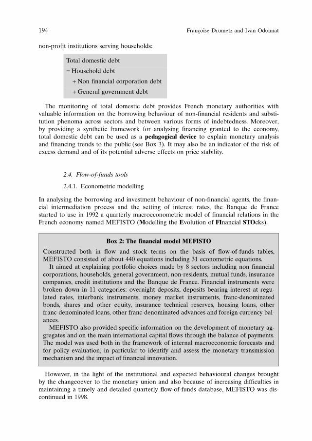
non-profit institutions serving households:
Total domestic debt
= Household debt
+ Non financial corporation debt
+ General government debt
The monitoring of total domestic debt provides French monetary authorities withvaluable information on the borrowing behaviour of non-financial residents and substi-tution phenoma across sectors and between various forms of indebtedness. Moreover,by providing a synthetic framework for analysing financing granted to the economy,total domestic debt can be used as a pedagogical device to explain monetary analysisand financing trends to the public (see Box 3). It may also be an indicator of the risk ofexcess demand and of its potential adverse effects on price stability.
2.4. Flow-of-funds tools
2.4.1. Econometric modelling
In analysing the borrowing and investment behaviour of non-financial agents, the finan-cial intermediation process and the setting of interest rates, the Banque de Francestarted to use in 1992 a quarterly macroeconometric model of financial relations in theFrench economy named MEFISTO (Modelling the Evolution of FInancial STOcks).
Box 2: The financial model MEFISTO
Constructed both in flow and stock terms on the basis of flow-of-funds tables,MEFISTO consisted of about 440 equations including 31 econometric equations.
It aimed at explaining portfolio choices made by 8 sectors including non financialcorporations, households, general government, non-residents, mutual funds, insurancecompanies, credit institutions and the Banque de France. Financial instruments werebroken down in 11 categories: overnight deposits, deposits bearing interest at regu-lated rates, interbank instruments, money market instruments, franc-denominatedbonds, shares and other equity, insurance technical reserves, housing loans, otherfranc-denominated loans, other franc-denominated advances and foreign currency bal-ances.
MEFISTO also provided specific information on the development of monetary ag-gregates and on the main international capital flows through the balance of payments.The model was used both in the framework of internal macroeconomic forecasts andfor policy evaluation, in particular to identify and assess the monetary transmissionmechanism and the impact of financial innovation.
However, in the light of the institutional and expected behavioural changes broughtby the changeoever to the monetary union and also because of increasing difficulties inmaintaining a timely and detailed quarterly flow-of-funds database, MEFISTO was dis-continued in 1998.
194 Francoise Drumetz and Ivan Odonnat

2.4.2. The table of financing and investment (TFI)
In the meantime, the Banque de France has also developed a table of financingand investment (TFI) at the national level. The French TFI – Tableau des finance-ments et des placements – contains consistent information on the instrument andsectoral breakdowns of financing and on the financial portfolio choices of economic
The integration of analysis of extended monetary and credit aggregates 195
Table of Financing and Investment
FINANCIAL INVESTMENT BY NON-FINANCIAL RESIDENTS
SHORT-TERM DEPOSITS AND SECURITIESVIS-A-VIS RESIDENT MFIs (A)
Currency in circulation and short-term deposits
Debt securities < 2 years, MMF units and repos
OTHER SHORT-TERM DEPOSITS AND SECURITIES (B)
Other deposits (cross border deposits, etc.)
Other short-term securities (commercial paper, etc.)
MEDIUM- AND LONG-TERM INVESTMENTS (C)
Deposits with agreed maturity > 2 years
Bond-type investments
Equity-type investments
TOTAL INVESTMENT (D = A + B + C)
FINANCING GRANTED TO NON-FINANCIAL RESIDENTS
Loans (E)
�1 year
>1 year
Loans granted by non-residents
Private sector deposits with the central government (F)
Market financing (G)
�1 year
>1 year
TOTAL DOMESTIC DEBT(monetary statistics definition) (H = E + F + G)
Change to financial statistics (I)
TOTAL DOMESTIC DEBT(national accounts definition) (J = H + I)
SHARES AND OTHER EQUITY (K)
TOTAL FINANCING (L = J + K)

agents. It thus provides a synthetic view of the investments and net asset statementof non-financial agents which is quite useful in the evaluation of monetary policyeffects.
Up to the start of Stage III of EMU, the TFI was considered as an intermediateanalytical tool between national financial accounts and monetary aggregates. Availableon a quarterly basis, it provided a comprehensive picture of the financial behaviour ofnon-financial residents, allowing a simultaneous analysis of money and investment ag-gregates, total domestic debt and equity financing developments.
Compared to the MEFISTO experience, the TFI approach seemed more promisingin terms of maintenance costs, data availability and timeliness. Accordingly, the TFIpresentation was reviewed to take into account the Stage III statistical requirementsand the full implementation of ESA 95. It now covers the non-financial resident popula-tion (general government, non-financial corporations, households and non-profit institu-tions serving households), which differs from the money-holding sector to the extentthat the former includes the central government but not the non-monetary financialinstitutions. Henceforth, the French contribution to M3 cannot be directly derived fromthe TFI 1.
Furthermore, the TFI covers a larger spectrum of financial instruments than themonetary statistics. Regarding the liability side, only a few changes have been made tothe former presentation, as the consistency with other financing indicators is ensured bythe inclusion of the total domestic debt components and an item reflecting the changefrom nominal to market value. On the assets side, the reference to both national ac-counting standards and the definition of monetary instruments has led to a breakdownin three categories: short term deposits and securities vis-a-vis resident MFIs (monetaryassets), other short term deposits and securities (non monetary liquid assets) and med-ium and long term investments. The French TFI is shown hereafter with a detailedinstrument breakdown.
3. The integration of extended money and credit aggregatesin the analysis of the Banque de France: three “case studies”
3.1. Monetary developments in 1993
In 1993, the main aggregates used as monetary policy indicators showed contrastingtrends. Lending and, to an even greater extent, the money supply aggregate M3, whichwas the target aggregate for monetary policy, started to contract from the middleof 1993. On the other hand, there was a sustained increase of about 4% in total domes-tic debt throughout the year. Meanwhile, the investment aggregates showed exception-ally rapid growth.
These contrasting developments reflected massive switching between different typesof financial investments and different forms in financing. Several clearly identified fac-tors were behind these changes (see Box 3).
196 Francoise Drumetz and Ivan Odonnat
1 Branthomme, Marchal and Odonnat (2000)

Box 3: What happened in 1993?
1. While the 1993 target range for growth in M3 had been set at 4%–6.5%, theaggregate actually shrank by 2.2%.
Broad money aggregate M3
Source: Banque de France
This break in the M3 trend in 1993 can be explained by:
� the effect of the economic slowdown, as the target range was set with referenceto 1993 GDP growth forecasts that were not achieved (nominal GDP growthfor 1993 stood at 1.5% whereas 5.5% growth had been expected); this resulted inless demand for transaction balances and for credit;
� the flattening of the inverted yield curve through the decrease of short-term rates,which made short-term maturities less attractive; short-term investments carryingmoney market interest rates accounted for about 45% of M3;
� discretionary factors which encouraged the household and corporate sectors toconsolidate their monetary holdings by enlarging the supply of savings vehiclesavailable (launch of the “Balladur” loan; greater reliance on bond issues, insteadof Treasury notes and bills, to finance Government debt; privatisation pro-gramme); moreover, tax changes diminished the attraction of MMF units thatmade up 30% of M3.
Adjusted for the discretionary factors mentioned above, the 1993 change in M3stood at approximately 1.8%, still far below the target range of 4%-6.5%, but com-parable to the growth of nominal GDP.
2. The flattening of the yield curve and the discretionary factors led to a massivetransfer of monetary assets into financial investment assets covered by the P1 (con-tractual savings), P2 (bonds) and P3 (equities) aggregates which showed very rapidgrowth in 1993 (20.8%, 29.3% and 31.1% respectively). Given the outstanding li-quidity of French capital markets, and especially the liquidity of mutual funds inbonds and equities, this transfer of assets into longer-term savings vehicles was notseen by monetary authorities as the outright destruction of money in favour of long-term savings.
The integration of analysis of extended monetary and credit aggregates 197
��
��
��
�
�
�
�
�
��
��
���� � ���� ������ ������ ���� � ���� ������ ������ ���� � ���� ������ ������ ���� � ���� ������ ������ ���� � ���� ������ ������
�������� ����� �� ��� �� ������� � ������ �� ��

3. The annual growth rate of total domestic debt was 4% or more throughout 1993,which was significantly higher than the nominal GDP growth. Here again, massivesubstitution had occurred but, because of the specific features of this aggregate, itsevolution had not been affected. As regard the pattern of financing raised and the typeof borrowers, while loans granted to the private sector contracted slightly by 0.4%,financing through domestic debt issues grew strongly (+15%), particularly governmentborrowing on the bond market (+29%); the government borrowing requirement – in-cluding the “Balladur” bond – was, therefore, substituted for the requirements of othereconomic agents, reflecting the effect of automatic stabilisers during a cyclical slow-down and the structural deterioration of the government’s finances.
The monetary policy strategy set by the Monetary Policy Council of the Banque deFrance for 1994 took into account these developments and the uncertainty surroundingthe evolution of M3 in 1994:
� the Council considered that the abrupt deviation of M3 from its medium-term growthtrend was due to exogenous causes and did not invalidate the targeting of this aggre-gate as the medium-term reference for France’s monetary policy; however, owing tothe fact that the discretionary factors which explained the deviation of M3 from itsmedium-term trend in 1993 might also come into play in 1994, no annual target rangewas set for M3 growth: instead, the Council set a medium-term growth trend of 5%for M3, in keeping with the potential for 2.5% to 3% medium-term real non-infla-tionary GDP growth and price rises of less than 2%;
� total domestic debt was singled out as a prominent indicator for monetary policy,particularly in times of major structural changes in monetary and capital markets,savings patterns and government financing. As evidenced in 1993, shifts between bor-rowing from credit institutions and market financing, portfolio shifts induced by non-monetary measures such as changes in tax or government funding policies, or shiftsbetween the borrowing requirements of economic agents can impinge directly upongrowth in monetary aggregates while having no impact on total domestic debt.
The definition of a medium-term growth trend for a monetary aggregate and themonitoring of total domestic debt remained major features of the French monetarypolicy strategy until 1999.
3.2. Monetary developments in 1996
Monetary developments in 1996 underlined once again the need to have recourse tobroader concepts.
Box 4: What happened in 1996?
1. M3 experienced a trend reversal in 1996. The annual 4.6% growth of M3 in 1995gave way to a 3.3% contraction in 1996.
Motivated by monetary policy as well as regulatory considerations, portfolio deci-sions made by non-financial economic agents had a strong influence on the M3 ag-gregate. Massive shifts in investment flows were sparked off by the unprecedentedamplitude and speed of the fall in short-term market interest rates since the autumn
198 Francoise Drumetz and Ivan Odonnat

of 1995 and by the cancellation of the tax advantage granted on capital gains onsales of MMF units which had already been reduced in previous years.
2. This change in investment flows was amplified by new developments regarding hous-ing saving plans, a component of the P1 investment aggregate. These instruments exhibitspecific features: they offer a loan option; their interest rate is fixed and set by the gov-ernment; they can be held up to ten years although the initial maturity is four years.However, over the past years, housing saving plans proved to be more and more liquid.As it is possible to renew the contract at maturity for short-term periods up to a max-imum of six additional years and because housing saving plans were paying a relativelyhigh interest in the mid-nineties, households started to use them as a substitute formonetary assets. Indeed, P1 showed a very strong twelve-month increase of almost 18%at the end of 1996. Therefore, the M3+P1 aggregate expanded by 1.5% in 1996. P2 andP3 also posted strong growth figures (16% and 25% respectively).
Non-financial resident holdings of MMF units and housing saving plans
Source: Banque de France
3. Annual growth in total domestic debt fell from 5.9% in 1995 to 3.1% in 1996. Thisoverall slowdown mainly reflected a deceleration in growth of government debt to6.7% at end – 1996 from 15.1% a year earlier, in line with the gradual consolidationof public finances. Loans granted by all resident financial institutions to non-financialresidents contracted by 1.8% at the end of 1996. This evolution reflected in part amove towards greater disintermediation, companies taking advantage of low marketinterest rates: a third of their debt reduction vis-a-vis credit institutions was compen-sated for by increased securities issuance. Moreover, the corporate sector posted avery substantial self-financing rate.
These developments had some implications for the definition of the monetary policystrategy of the Banque de France for 1997 and 1998.
The Council announced that given the disruptions which had recently affected M3, hewould keep a very close eye on the M1, M2, M3 and M3+P1 aggregates as expressions ofthe underlying growth of the money supply, in order to establish a synthetic estimate ofoverall monetary developments. Particular attention would be paid to the growth of the
The integration of analysis of extended monetary and credit aggregates 199
���
���
�
��
��
��
��
��
� � � � � � � � �
� ���������� ���� ����� � ����� ������� � ���
������������� ���� �� ��

M3+P1 aggregate, since this type of investment, particularly housing savings plans with aresidual maturity of one year or less, constituted a very close substitute for monetary assets.
M3 and M3+P1
Source: Banque de France
3.3. Financing developments in 1999
The rise in the overall indebtedness of resident non-financial agents has acceleratedsince mid-1998, notably via faster credit growth. Thus, the trend towards disintermedia-tion observed since the mid-1990s – resulting from the more rapid expansion of marketfinancing – was slightly less accentuated in 1999.
Box 5: Recent trends of financing flows in France
1. The annual growth rate of total domestic debt has increased since the mid-1998.The annual growth rate of total domestic debt accelerated from 3.4% in June 1998to 7.2% at the end of 1999, the highest rate ever reached since the mid-1990s. Therise was driven by the private sector, while in the previous period of acceleration(December 1994-April 1996), the main force was the general government.
Contribution of economic sectors to the annual growth of total domestic debt
Source: Banque de France
200 Francoise Drumetz and Ivan Odonnat
��
��
�
�
�
�
�
���� � ��� ����� ����� ���� � ��� ����� ����� ���� � ��� ����� ����� ����
�� �����
�������� ����� �� ��� �� ������� � ������ �� ��
�
�
�
�
�
�
�
�
�� �� ��� �� �� �� ��� �� �� �� ��� �� �� �� ��� � �� � ��� �� �� ��
��������� ������� ���������� ��� !����!�� ���"����!��� #���� �����!� �$�
���

Indeed, the annual growth of the general government debt slowed down with a netflow decreasing from EUR 83.3 billion in 1996 to EUR 14 billion in 1999, in connec-tion with the reduction of the general government deficit.Conversely, the private sector indebtedness rose significantly. Several factors mayexplain this trend reversal:
� First, the lagged positive effect of the reduction in interest rates. Between 1995and 1999, the three-month interbank interest rate decreased from 5.6% to 3.4%and the 10-year government bond interest rate declined from 6.7% to 5.3%. How-ever, most of the decrease in short-term interest rates was effective by the begin-ning of 1996. In addition, the rise recorded in long-term interest rates over 1999(from 3.9% to 5.3%) did not prevent a further acceleration in the private sectordebt growth:
Growth of the private sector debt and interest rates
Source: Banque de France
� Second, the non-financial corporations’ financing strategy also played an impor-tant role. Their self-financing ratio went back to 87.6% and 80.6% in 1998 and1999 respectively, after having reached historical highs in the mid-1990s (close to100%), following a rise in productive investment. At the same time, their debtratio started to increase again after a continued decline between 1993 and 1998.Namely, companies seem to have replaced equity financing by debt financing inthe recent years, as a counterpart of their equipment purchases.
� Third, in the case of households, the strengthening of indebtedness trends alsorelates to sustained demand for consumption goods and real estate since 1996. Onaverage, the annual growth rate of individual housing purchases reached 4.2% innominal terms over the period 1996–1999, compared to 1.2% between 1993 and1995. At the same time, the annual growth rate of household consumption in-creased from 1.6% to 2.5%. These additional expenses were partially covered bydebt financing. Thus, the household debt ratio increased significantly from 52% in1996 to 54.2% in 1999.
The integration of analysis of extended monetary and credit aggregates 201
�
�
�
�
�
��
��
���� ���� ���� ���� ���� ���� ���� ���� ����
������ ��������� ���� ������ ���������� ���� ���� ����� ���!�� ���� �" #������ $���� ���� ����
���

2. The financial disintermediation process initiated in the eighties slowed down in 1999Such developments can be measured by analysing the share of loans in the non-financial residents total debt. Accordingly, the share of loans in total domestic debtremained stable in 1999 after a continued decrease since the mid-1990s:
� over the period 1994–1999, loans granted by resident financial institutions to non-financial residents grew at a lower pace than other indebtedness forms. On aver-age, the annual growth rate of the former stood at 1.9% compared to 10.2% formarket financing and 10.7% for loans granted by non-residents. Henceforth, theshare of domestic loans in total domestic debt continuously declined, from 63.5%at the end of 1993 to 52% in 1999, while the share of market financing increasedfrom 29.7% to 38.5% and that of foreign loans rose from 4.8% to 6.8%. Thesetrends relate, in particular, to the behaviour of non-financial corporations. Thelatter tend to favour either market financing because in the recent past it hasappeared less costly than bank financing given the inertia of retail bank interestrates compared to market interest rates, or foreign financing in the form of loansgranted through direct investments in a context of increasing internationalisationof the French economy;
� however, the share of loans in total domestic debt remained stable in 1999, as thegrowth of loans granted by monetary financial institutions got momentum. Thedemand for credit addressed by small and medium size enterprises was indeedstronger because of the economic activity recovery as well as because of lowerlending bank interest rates. Meanwhile, large firms most likely continued to fa-vour market financing for mergers and acquisitions or, to a lesser extent, for theconstitution of precautionary holdings before the Y2K changeover.
Disintermediation and growth of domestic loans
Source: Banque de France
4. Lessons for monetary analysis in the euro area
4.1. Monetary analysis under the first pillar
The first pillar of the strategy of the Eurosystem confers a prominent role to money,signalled by the announcement of a reference value for broad monetary growth, and
202 Francoise Drumetz and Ivan Odonnat
��
��
��
��
��
��
��
��
��
���� � ��� ���� � ��� ���� � ��� ���� � ��� ���� � ��� ����
�
�
�
�
�
�
�
�
�
�
����� ������� �� �������� � ������� ������ ����� � ���� ��!���� ���� "����#��� ����$ %�� �� ���& �# ���� �� ����� "���#�#��� ����$
������

reflecting the monetary origins of inflation over the medium term. The Council of Gov-ernors has emphasized that “the reference value does not entail a commitment on thepart of the Eurosystem to correct mechanistically deviations of money growth from thereference value. Rather, monetary developments are thoroughly analysed in relation tothe reference value in order to ascertain their implications for the outlook for pricestability over the medium term” 2.
Therefore, the announcement of the reference value represents a commitment onthe part of the Eurosystem to thoroughly analyse and explain monetary develop-ments and their role in policy decisions. Thus, the first pillar encompasses a broaderrange of analyses of monetary and credit aggregates and of analytical tools (e.g. amoney demand function), even if not all of the underlying monetary analysis ispublished.
4.2. Proposals for additional indicators and analytical tools
In the context of a deregulated market economy that is largely open to financial inno-vation, it may also be important to analyse interactions between money, other forms ofinvestment and financing, and to interpret diverging trends in these variables.
In this regard, one should mention first the work already accomplished by theESCB within the framework of financial accounts, which aims at building a euro areaquarterly table of the financing and investment flows of non-financial agents. Theeuro area TFI, which is close to the French one in concept but differs from it in thatit makes an explicit reference to the monetary aggregates, is to be released in thenext few months.
The creation of a total domestic debt indicator for the euro area could also pro-vide a solution to these needs, like the indicator used by the Banque de France totrack financial developments in France. Such an indicator would make it possible,for internal purposes, to track developments in every form of debt financing in theeuro area simultaneously, within a single conceptual framework, as a supplement tothe indicators based on the MFI sector balance sheet. This addition would thusmake it easier to understand the monetary and financial developments in the euroarea.
The construction of such an indicator at the euro area level would also be consistentwith the definition and the implementation of a euro area TFI. Although narrower inscope than the table of financing and investment flows, since it would be limited todebt financing, a euro area total debt would nevertheless have a crucial advantage formonetary policy in that it can be produced on a monthly basis. In fact, this indicatorwould be based on data taken from the MFI sector balance sheet and security issuesstatistics, which are also available at short notice in most member states of the mone-tary union.
The integration of analysis of extended monetary and credit aggregates 203
2 “Review of the Quantitative Reference Value for Monetary Growth”, ECB Press Release,2 December 1999.

Annexes
Money and investment aggregates
Outstanding amounts Year-on yearFRF billion EUR billion % changes (a)
1998 1998 1997 1998
Banknotes and coins 265.0 40.4 1.1 1.6Franc-denominated overnight deposist 1735.7 264.6 7.4 3.8
M1 2000.7 305.0 6.5 3.5
M2 – M1 1784.2 272.0 9.2 5.5“A” passbooks 709.1 108.1 3.0 1.4“Blue” passbooks 99.7 15.2 4.2 3.7Housing savings accounts 168.6 25.7 5.6 4.5Industrial development accounts 229.6 35.0 8.1 5.4People’s passbooks 237.5 36.2 20.1 16.0Youth passbooks 31.5 4.8 17.9 4.3Taxable passbooks 308.3 47.0 24.3 9.3
M2 3784.9 577.0 7.8 4.4
M3 – M2 1744.9 266.0 – 8.2 – 0.9Foreign currency deposits and negotiable debtsecurities
124.0 18.9 4.2 12.2
Time deposits (b) 317.5 48.4 –12.8 – 1.6Loan notes and savings certificates 135.1 20.6 – 3.8 –13.4CDs and negotiable medium-term notes issuedby banks
264.4 40.3 5.6 – 6.5
Bills and negotiable medium-term notes issued byfinancial societies and specialised financial institutions
11.2 1.7 –39.0 2.1
MMF units 885.5 135.0 –11.3 2.1Securitised vehicle units � 5 years 7.2 1.1
M3 5529.8 843.0 2.0 2.7
M4 – M3 93.8 14.3 51.9 –25.8Negotiable treasury bills 78.1 11.9 80.6 –27.2Commercial paper and negotiable medium-term notes
15.7 2.4 –20.3 –16.9
M4 5623.5 857.3 2.8 2.0
Housing savings schemes 1146.6 174.8 13.8 8.6Other savings accounts (c) 22.3 3.4People’s savings plans 679.2 103.5 12.6 3.4– of which: insurance companies 177.4 27.0Guaranteed mutual fund units 167.3 25.5 39.3 19.1Capital accumulation certificates 311.1 47.4 3.6 – 0.6
P1 2326.5 354.7 13.6 6.4
Bonds 811.5 123.7 –16.6 – 2.3Life insurance investments 2908.0 443.3 17.8 12.0Bond mutual fund units 563.3 85.9 – 5.4 5.8
P2 (base 80) 4282.8 652.9 5.3 8.2
Shares 23384.0 4479.6 27.4 28.2Equity mutual fund units 332.9 50.8 36.5 34.9Composite mutual fund units 330.8 50.4 32.1 29.4Other mutual fund units (d) 245.9 37.5 28.5 23.0
P3 (base 80) 30293.5 4618.2 27.6 28.3
(a) At end-December(b) Time accounts, unavailable factoring accounts and forward securities transactions(c) Cash deposits on personal equity plans, savings contracts with savings and lending institutions and other regu-lated savings accounts(d) Employee mutual funds, venture capital mutual funds, future mutual funds and investment trusts
Source: Banque de France
204 Francoise Drumetz and Ivan Odonnat

Total domestic debtBreakdown by instruments
(end-of-period outstanding amount in EUR billions and percentage change)
Amount Twelve-month rate of growth
Aug. 00 Dec. 98 Dec. 99 July 00 Aug. 00
Total domestic debt 2176.8 4.8 7.2 5.6 5.8Households (a) 487.7 3.7 8.0 7.5 7.1�1 year 23.8 6.4 8.9 9.6 11.7>1 year 463.9 3.5 8.0 7.4 6.8Non-financial corporations 900.3 5.4 11.4 8.0 8.8�1 year 330.8 5.4 11.5 12.5 14.0>1 year 569.4 5.4 11.3 5.5 5.9General government 788.8 5.0 2.5 1.7 1.8�1 year 93.1 2.7 –12.9 2.0 1.5>1 year 695.7 5.3 4.8 1.7 1.8Loans obtained from resident FI (b) 1116.8 1.4 5.2 5.6 5.8Households (a) 487.7 3.7 8.0 7.5 7.1�1 year 23.8 6.4 8.9 9.6 11.7>1 year 463.9 3.5 8.0 7.4 6.8Non-financial corporations 518.9 2.3 5.9 6.9 8.0�1 year 138.3 –3.1 0.1 8.9 10.4>1 year 380.5 4.3 7.9 6.2 7.2General government 110.3 –7.9 – 6.0 –7.1 –8.1�1 year 10.7 –1.9 – 9.8 8.8 3.0>1 year 99.6 –8.5 – 5.5 –8.5 –9.1Loans obtained from non residents (c) 159.8 10.3 14.0 9.9 10.7Market financing 862.7 9.1 8.6 4.8 5.0Non-financial corporations 221.6 11.1 25.0 9.4 9.2�1 year 51.2 27.9 32.5 26.8 29.6>1 year 170.4 7.8 23.3 5.0 4.2General government 641.1 8.6 4.1 3.3 3.6�1 year 45.1 4.9 –28.5 –2.6 –0.4>1 year 596.0 9.0 7.1 3.7 3.9Private sector deposits with the central government 37.4 1.6 7.7 5.2 3.2
(a) Households + non-profit-making institutions in the service of households(b) FI (Financial institutions) = Monetary financial institutions + other financial intermediaries(c) Loans between units of different companies + loans obtained through direct investments + commercial loans
Source: Banque de France Produced 28 September 2000
Table of Financing and Investment(in EUR billions)
Outstandingamount1999Q4
Flow2000Q1
Outstandingamount2000Q1
FINANCIAL INVESTMENTBY NON-FINANCIAL RESIDENTS
SHORT-TERM DEPOSITS AND SECURITIESVIS-A-VIS RESIDENT MFIs (A)
841.1 – 0.5 846.6
Currency in circulation and short-term deposits 650.4 –11.2 639.7Currency in circulation 39.9 0.0 39.9Overnight deposits 292.2 – 7.2 285.3Savings passbooks 274.0 – 1.4 272.6Deposits with agreed maturity �2 years 33.4 1.3 34.9Deposits of the central government 10.9 – 3.9 7.0
The integration of analysis of extended monetary and credit aggregates 205

(Table continued)(in EUR billions)
Outstandingamount1999Q4
Flow2000Q1
Outstandingamount2000Q1
Debt securities �2 years. MMF units and repos 190.7 10.7 206.9Debt securities �2 years 50.6 3.9 54.5MMF units 131.4 3.9 140.5Repurchase agreements 8.7 2.9 11.9
OTHER SHORT-TERM DEPOSITSAND SECURITIES (B)
73.9 0.3 74.2
Other deposits (cross border deposits, etc.) 53.3 0.0 53.3
Other short-term securities (commercial paper, etc.) 20.6 0.3 20.9
MEDIUM- AND LONG-TERM INVESTMENTS (C) 4743.0 23.0 4937.7
Deposits with agreed maturity > 2 years 292.9 – 7.3 285.6Bond-type investments 853.5 14.3 866.2Bonds 114.7 – 0.3 110.1Other debt securities > 2 years 19.4 0.1 19.4Bond mutual funds 73.0 0.4 69.2Guaranteed mutual funds 35.4 0.8 33.9Insurance technical reserves 611.0 13.3 633.6
Insurance people’s savings plans 29.3 1.5 33.8Other life insurance investments 581.7 11.8 599.8
Equity-type investments 3596.6 16.0 3785.9Quoted shares 667.0 3.5 710.3Other equity 2712.6 8.7 2845.8Equity mutual funds 87.2 1.0 91.0Composite investment mutual funds 49.3 2.9 55.3Other mutual funds 80.5 – 0.1 83.5
TOTAL INVESTMENT (D = A + B + C) 5658.0 22.8 5858.5
FINANCING GRANTEDTO NON-FINANCIAL RESIDENTSLoans (E) 1235.3 23.3 1257.6�1 year 157.8 11.1 169.5>1 year 928.3 7.0 933.7Loans granted by non-residents 149.2 5.2 154.4Private sector deposits with the central government
(F)38.0 – 2.1 35.9
Market financing (G) 815.6 5.2 822.3�1 year 76.1 2.6 78.8>1 year 739.5 2.6 743.5
TOTAL DOMESTIC DEBT(monetary statistics definition) (H = E + F + G)
2088.8 26.4 2115.8
Change to financial statistics (I) 38.3 ns 38.8
TOTAL DOMESTIC DEBT(national accounts definition) (J = H + I)
2127.2 26.4 2154.6
SHARES AND OTHER EQUITY (K) 4079.0 14.5 4256.2Quoted shares 1295.1 8.8 1314.6Other equity 2783.9 5.7 2941.6
TOTAL FINANCING (L = J + K) 6206.2 40.9 6410.8
206 Francoise Drumetz and Ivan Odonnat

References
Banque de France, Annual ReportsBordes, C. and Strauss-Kahn, M.O. [1988], “Dispositif de controle monetaire en France et chocs sur
la vitesse dans un environnement en mutation”, Economies et Societes n� 1, 105–154.Bordes, C. and Strauss-Kahn, M.O. [1989], “Cointegration et demande de monnaie en France“, Cah-
iers economiques et monetaires, n� 34, 161–197.Boutillier, M. and Cordier, J. [1995], “One look at the way the French financial system has adapted
to the new monetary policy regime”, Banque de France, paper prepared for the Bank of Korea5th central banking seminar, November.
Branthomme, P., Marchal, D. and Odonnat, I. [2000], “Les indicateurs monetaires et financiers acaractere national suivis par la Banque de France en Union monetaire”, Banque de FranceBulletin n� 81, September, 53–65.
Cordier, J. and Jaillet, P. [1993], “The business cycle and financial changes in France – Some effectsof and implications for monetary policy”, BIS C.B. 392-Changes in the business cycle and theimplications for monetary policy, April, 83–111.
Enfrun, B. [1992], “Mutations financieres et elargissement du cadre de l’analyse monetaire”, Cahierseconomiques et monetaires, n� 40, 225–239.
Enfrun, B. [1994], “L’endettement interieur total, instrument d’analyse global de la monnaie et desfinancements”, Banque de France Bulletin-Quarterly “Studies” Supplement-3rd quarter, 29–39.
Gervais, E. [2000], “Trends and Structure of Financing Flows in France and the Euro Area”, Ban-que de France Bulletin Digest-n� 83, 19–29.
Henry, J. and Sicsic, P. [1992], “Stationnarite autour d’une tendance deterministe coudee de la vitessede circulation de la monnaie”, Banque de France, paper prepared for the 9th banking economicsinternational seminar-Nantes, June.
Icard, A. and Drumetz, F. [1994], “Developpement des marches de titres et financement de l’econo-mie francaise”, Banque de France Bulletin-n� 6, June, 83–107.
MEFISTO team, [1992], “A model of the French financial system at the Bank of France-MEFISTOVersion 1”, Economic modelling-Vol. 9-n� 3, July, 211–252.
Patat, J.-P. [1993], “Monnaie, institutions financieres et politique monetaire”, Economica, 5th edition.Pfister, C. and Grunspan, T. [1999], “Some implications of bank restructuring for French monetary
policy”, BIS Conference Papers-Vol. 7, March, 188–207.Shigehara, K. [1996], “The options regarding the concept of a monetary policy strategy“, OECD,
paper prepared for the Deutsche Bundesbank symposium on “Monetary Policy Strategies inEurope“, April.
The integration of analysis of extended monetary and credit aggregates 207

1. Reasons for focusing on flow of funds analysis1
Monetary and financial analysis as conducted by central banks has evolved over thelast century in order to remain in touch with an increasingly complex economic andfinancial world. In a sense, flow of funds analysis might be seen as the final stage of along haul during which the most relevant pieces of information for central banks’ as-sessment have been pursued. Although the events described in this section are overlyrough and simplistic, they may help place flow of funds analysis in an appropriate per-spective.When monetary policy began to be implemented in a modern sense, central banksdid not need to go too far to collect information about the financial world. Indeed,their balance sheets contained fundamental data for analysing liquidity and credit con-ditions in the economy and the external sustainability of the economic situation. More-over, in some countries central banks played a key role in providing finance to thegovernment, thus influencing most significantly the economic cycle and inflationary pro-spects. Even if data had to be properly interpreted, they were immediately available,with no delay and no estimated components or errors.Afterwards the financial system developed much further and the population’s eco-nomic welfare increased substantially, with both factors promoting household saving.Financial markets, especially those for public debt, also expanded and monetary policytook a more stabilising role. As a result of these factors, the central bank’s balancesheet lost some of its past importance to the benefit of credit institutions’ balancesheets. Households and firms depended crucially on those entities to obtain finance andmost of their saving was also invested in them. Moreover, currency and bank deposits(money) were the key variables to monitor if monetary policy aimed to ensure pricestability. A very sound theoretical and practical framework was duly established, sup-ported by the collection of data from credit institutions through which almost all rele-vant financial information was obtained.Finally, in the last two decades, other financial intermediaries emerged and expandedand the size of financial markets -not only for trading with public debt – increased
Flow of funds analysis in the experienceof the Banco de Espana
Juan Ma Penalosa and Teresa Sastre*
Banco de Espana
* Helpful comments from our discussant Cees Ullersma and the participants of the ECB Mone-tary Analysis Seminar are gratefully acknowledged.1 In this paper the terms “flow of funds” and “financial accounts” are used indistinctively, both
referring to the data on financial flows and outstanding amounts classified by financial instrumentand economic sector.

forcefully. Disintermediation, financial deregulation and liberalisation, and internatio-nalisation were the major forces behind the outstanding changes in finance. Thesefactors reinforced each other making the whole process unstoppable. Whereas theauthorities might be seen to have ignited the initial stages of the process, they havebeen somewhat overpowered subsequently by the speed and strength of the ensuingchanges.As concerns traditional monetary and financial analysis, centred on money and loans,these changes advised taking a wider perspective of the financial variables. The mainconsequences of these factors for monetary and financial analysis can be summarised asfollows:
� A growing share of saving is not reflected in the MFIs’ balance sheets. Direct equitypurchases on the market (also encouraged recently by Internet access), insuranceproducts and, in particular, mutual funds have partly replaced traditional bankingdeposits. Table 1 shows that in 2000 only one-third of the financial assets held bySpanish households was invested in currency and bank deposits as compared withtwo-thirds at the beginning of the decade.
� Capital markets and financial intermediaries other than credit institutions are playingan increasingly important role in channelling financial resources from savers to inves-tors. In the Spanish case, loans from credit institutions only accounted for 26% ofnon-financial corporations’ total increase in liabilities in 1999, as compared with 36%ten years earlier. In this case, disintermediation is not observed in the issuance ofbonds, which is still very scarce, but in the resort to the issuance of equities.
� Financial innovation and the development of financial markets has made it possiblefor banks to offer new and more attractive combinations of liquidity and risk in theirproducts. In this respect, it is very difficult to disentangle where to place the border-line between monetary (liquid) and non-monetary assets. The distinction betweenassets mainly used for a transactions motive or for investment, or between low-riskvery liquid assets and riskier and less-liquid ones, has become blurred and compli-cates to define what money really is.
All these major changes do not recommend abandoning all previous indicators andthe preceding framework. It merely advises scaling down their significance and not
210 Juan Ma Penalosa and Teresa Sastre
Table 1
Outstanding Financial Assets of Households andNon-Profit Institutions Serving Households (NPISH)
Breakdown as percentage of total (a)
Memorandum itemAs % GDP (b)
1990 1995 1999 2000 IIIQTotal 100,0 100,0 100,0 100,0 191,0Currency, deposits and securities 68,0 55,4 34,6 36,7 70,1Shares and other equity 14,5 28,6 51,6 48,1 91,9Insurance technical reserves 7,6 10,1 10,7 11,9 22,8Other accounts 9,9 5,9 3,1 3,3 6,2
(a) The 1990 data were compiled following the methodological guidelines of ESA 79, and the 1995and 1999 data, following ESA 95.
(b) Referred to 2000 IIIQ.

neglecting other sources of financial information. The financial system is changing ra-pidly and central banks need to adapt their way of dealing with financial information.Bank assets and liabilities will continue to play a central role in monetary and financialanalysis, but it should be recognised that other relevant intermediaries cannot be side-lined. A wider framework of analysis thus seems to be better suited to cope with thisincreasingly complex world.This paper examines how information contained in financial accounts may contri-bute to improving our knowledge of the monetary and financial conditions faced byeconomic agents, making a special reference to the work conducted at the Banco deEspana in this respect. Section 2 outlines the main advantages and drawbacks of pla-cing financial accounts at the forefront of a central bank’s financial analysis. In Sec-tion 3 the Banco de Espana’s first steps in this direction are presented, while Section4 shows the potential improvements which are being considered. Finally, Section 5draws the conclusions.
2. Cons and pros of flow of funds analysis
2.1. Cons
The main disadvantages of flow of funds analysis are related to its complexity as a toolfor analysing monetary and financial developments. In fact, the great efforts made tobuild up domestic financial accounts have not run in parallel to the use of these ac-counts for policymaking. The lack of high-frequency data up until very recently may beone of the main reasons for this. In any case, once quarterly data are available it is tobe expected that more and better answers will be found to the relevant questions pol-icymakers ask.Difficulties in the analysis of financial accounts may be classified into two largegroups: the first includes all problems relating to the collection and processing of infor-mation; the second one is related to the informational content of flow of funds forfinancial analysis.Flow of funds data provide for an exhaustive collection of information of all eco-nomic sectors’ financial balance sheets, their financing and investment The first pro-blem is therefore how to obtain such a huge amount of data promptly and accu-rately. In contrast to the central bank’s balance sheet, whose information can beobtained daily or even instantaneously, or to the MFIs’ balance sheets, whosemonthly reports offer a detailed picture of their operations, the financial accounts ofthe economy can only be produced quarterly and with a significant delay. This im-plies that they do not provide yesterday’s or last month’s data but at most those ofthe last-but-one quarter.Moreover, financial accounts offer a fully closed and coherent picture in which, ulti-mately, several economic constraints are verified (e.g. for each instrument, net acquisi-tions by all sectors must equal net change in liabilities of all sectors). This allows theinformation from one sector to be used to complete that of a different sector, but italso entails the need to obtain or estimate the whole set of data in order to close thesystem coherently.It must also be assumed that flow of funds analysis is not fully based on observeddata. Actually, there are no primary data for a number of agents and transactions,
Flow of funds analysis in the experience of the Banco de Espana 211
and, in particular, for the most relevant sectors for spending decisions: householdsand non-financial corporations. Therefore, financial accounts contain several elementswhich are to some extent estimated. This introduces a certain degree of ambiguityinto the construction of financial accounts: whereas once money is defined, the uncer-tainty on how to measure it is reduced considerably, calculations of household savingare more the result of an intellectual process combining primary information andexpert judgement.This brings the discussion to another important issue. Are flow of funds data neutral?Namely, can we trust statisticians – when preparing the financial accounts – not toprejudge the subsequent monetary and financial analysis by juggling figures? Even ifexperts cannot be asked to ensure that the financial accounts are a pure reflection ofreality, analysts may demand that at least no bias be included in the way some financialtransactions are estimated or the whole system is closed. This is particularly relevant inthe household and non-financial business sector where the quality of information isfairly mixed: on one hand, there is very reliable and prompt information on their finan-cial transactions vis-a-vis MFIs; on the other, for transactions with securities the privatesector is considered the residual sector – as no primary information exists for it – andtherefore it is the one which has to adjust the likely differences between the instru-ments issued and the amount held by other sectors.As to the collection and availability of information, it should also be recalled thatthere are certain transactions and instruments whose measurement is particularly com-plex. This is the case of real assets, whose changes are very important when explainingthe economic and financial decisions of households. Although not a financial variable,the lack of an adequate measurement of housing wealth limits the assessment of house-holds’ financing and investment decisions stemming from financial accounts.Finally, an important element to be considered is that financial accounts follow a setof statistical principles (at present based on ESA 95) which sometimes may not providethe best basis for assessing certain monetary and financial developments. Faced withthese problems, users must choose between accepting the criteria of the accounts oradjusting specific items in order to obtain a more appropriate picture of the financialsituation. In the latter case, the fact we are dealing with a closed system of accountsmakes any adjustment in the original data a fairly complex task.The second group of problems relates to the way such a large amount of data can bemanaged to allow economic analysts to make sense of it. The underlying theoreticalrationale for this analysis is still weakly integrated with the assessment of financial con-ditions provided by financial accounts. This may be partly due to the fact that theoreti-cal relations embodied in this information have only been partially exploited whenmodelling relationships among financial and non-financial variables.Much research has been conducted in the past to explain the performance of moneyand credit. And despite significant obstacles, it has been notably successful. However,modelling different categories of financial assets and liabilities or broader aggregatesappears to be a much more difficult task. Many questions remain unanswered. Whatare the factors behind the demand for financial assets? Does the latter depend on thedemand for liabilities? Is it possible to identify the forces shaping portfolio shifts? Andwhat role do financial decisions play in spending? Therefore, the full exploitation offlow of funds possibilities requires strong research and a clear theoretical framework toorganise the huge amount of information available.
212 Juan Ma Penalosa and Teresa Sastre

2.2. Pros
The advantages of focusing on flows of funds to conduct financial analysis stem bothfrom the difficulties of making an assessment based on narrower and specific variablesand from the genuine pros of such an analysis.As commented above, money is a key variable in monetary and financial analysis,but confidence about its informational content has been gradually declining for the pasttwo decades. Money is almost impossible to define as financial innovations continuouslychange the features of liquid financial assets, obliging central banks to re-assess moneydemand on an ongoing basis. Although money is still important, increasing attentionhas to be paid to other financial variables in order to substantiate that information andenrich the analysis. Likewise, credit from the MFIs to the private sector is still relevantbut a full account of how non-financial corporations fund their activity also requiresconsidering the issuance of bonds and equity. Even data on lending to households maybe distorted by the growing importance of mortgage loan securitisation.Among the difficulties of dealing with the financial accounts, the large amount ofdata involved was mentioned earlier. At the same time, such information may providefor a deeper assessment of the economic and financial situation of the country. It pro-vides for the potential to recognise the interdependence between expenditure and port-folio allocation decisions and the interrelationships between different sectors’ behaviourin the various asset markets. Thus, ex-ante sectoral budget constraints of the type:
Gross Savings + Change in liabilities = Investment + Financial asset acquisition
induce several relationships among financial and non-financial variables within eachsector. Furthermore, there may still be some interdependence between spending andportfolio composition decisions. For instance, the fact that a good deal of wealth reva-luation has come from increases in the value of mutual funds, which can be easily liqui-dated, might have had an important influence on spending decisions in Spain. Further-more, the fact that some financial markets are not always cleared through interest rates(credit rationing is relatively common in bank lending) implies a binding constraint onthe non-financial decisions of economic sectors. This allows for financial variables notto be considered as endogenous, as is often assumed, permitting feed-back relationsbetween real and financial variables to be taken into account.At a minimum, financial data provide for an additional source of information toassess recent developments in real variables as it allows to conduct a cross-check ofreal-sector information. Actually, financial accounts provide us with some idea of netfinancial saving by sector, which can be compared with net borrowing/lending obtainedfrom the non-financial transactions accounts. This type of contrast is interesting sincefinancial and non-financial variables are to some extent independent sets of informationof a process in which agents take both real and financial decisions at the same time.Flow of funds analysis is also advantageous as it enables sector-by-sector assessmentof monetary and financial conditions. Such a sectoral perspective is difficult to obtainfrom the traditional variables, relating to money, credit and interest rates. Changes inthe monetary policy stance and the different channels of monetary transmission affectfinancial prices and quantities, but its impact on each economic sector may be quitedifferent. For example, the net financial position of a particular economic sector and itsportfolio composition affects its sensitivity to changes in interest rates. This sectoral
Flow of funds analysis in the experience of the Banco de Espana 213

approach, of a more microeconomic nature, is essential to fully understand the effectsof monetary policy on the economy2. Flow of funds analysis thus enables us to examineboth the financial performance by sector and the links between sectors following anypolicy decision or change in the institutional framework. This approach is thereforemuch more ambitious and far-reaching than that focused on specific monetary andfinancial variables.The importance of financial flows other than money and credit was explained beforeby the growing relevance of the disintermediation, deregulation and internationalisationof modern financial systems. Also, in the last two decades there has been an ongoingprocess of increasing investment by households in variable-yield instruments, such asequities and shares in mutual funds. These assets introduce new financial considera-tions, as fluctuations in their prices may have important repercussions for householdbehaviour. The so-called wealth effect is increasingly significant in a number of coun-tries whose economic developments are sometimes difficult to explain without somereference to that effect. By showing the proportion and performance of those assets,the financial accounts allow for an assessment of the potential implications of a changein asset prices. For example, in the Spanish case, almost one-half of financial assets heldby households -equivalent to slightly less than 100% of GDP- is invested in equitiesand other variable-yield securities (see Table 1).Flow of funds analysis also enables us to address an important source of concern forcentral banks: financial stability. Irrespective of their responsibility for banking supervi-sion, central banks and, in general, economic authorities are becoming increasingly wor-ried about the stability of the financial system. The traditional risks stemming fromsystemic considerations are now compounded by the much larger and more complexfinancial system in which economic agents conduct their activities and by the tighterlinks between different financial markets. Financial accounts show very relevant infor-mation about the health of sectoral balances, risks, vulnerabilities, potential effects fromchanges in exogenous variables, and so on.All the aforementioned reasons warrant implementing a thorough analysis of theinformation provided by the financial accounts, aiming at fully characterising financialconditions which affect the main economic sectors, assessing how monetary policy deci-sions are transmitted and examining the interrelationships between expenditure andportfolio asset allocation decisions3. Moreover, from the standpoint of a national cen-tral bank, there is also a timely reason to devote more resources to this task. The startof Monetary Union has led to the conduct of a single monetary policy which focuses ondevelopments across the whole euro area. Evidently, therefore, the performance ofmonetary and financial conditions in one single country cannot influence the monetarypolicy of the whole area. However, analysis of domestic conditions is useful from differ-ent points of view (see Banco de Espana (1999a)). For one thing, from the domesticviewpoint the assessment of the financial situation of the domestic sectors may help tounderstand economic developments thus allowing for the design of a proper policy mixat the national level as well as to assess financial stability issues. For another, such an
214 Juan Ma Penalosa and Teresa Sastre
2 Penalosa (1998) examined the effect of agents’ financial position in the transmission of mone-tary impulses. More recently, Cuenca and Saez (2000) analysed the sectoral income effect on thebasis of the data provided by the financial accounts.3 There is a fairly wide agreement among several authors that these are the main uses of the
flow-of-funds approach (see, for instance, Owen (1986) and Alho (1991)).
analysis could also be fruitful from the Eurosystem’s standpoint, as it complementsmonetary and financial analysis for the whole euro area, raising points of potentialinterest to other countries. Moreover, the domestic assessment may also be useful forchecking the consistency of the future European financial accounts, which are currentlyunder preparation.
3. First steps in the flow of funds analysis
Economic analysis requires promptness: though explaining the past is important, centralbanks need to know what is going on at present in order to provide an adequate judge-ment of the situation. Analysis should thus be based on promptly available data. How-ever, the more ambitious and numerous the variables to be measured, the more diffi-cult it is to comply with this requirement.Financial accounts represent a compilation of all financial flows of the economy clas-sified by sector and instrument. As these accounts are a closed and coherent system, ahuge amount of data is needed before the system can be fully closed. In the Spanishcase, regular publication of quarterly financial accounts started in 1999. Data are avail-able for the period 1987.I–1999.IV based on ESA 79 methodology and as from 1995.Iaccording to ESA 95 criteria. The quarterly financial accounts are published regularlywith a 100-day delay (slightly longer than three months), which is around 2–3 weeksafter the national accounts are available. This delay is not fully satisfactory but dueaccount should be taken of the fact that there are some sectors, such as insurance enti-ties or the external sector, whose information is only obtained with a significant lag.To cope with such a delay, two main measures have been taken. First, monthly indi-cators of liquidity – in a broad sense – and financing have been constructed. Theseindicators are largely drawn from the monthly MFIs’ balance sheets and are thereforeavailable with only a three-week delay. Second, an effort is made to estimate and extra-polate the performance of some assets and sectors for the most recent quarter, takinginto account the information which is readily available.In order to make a sensible assessment of the information, data have to be properlyarranged: relevant indicators must be selected and the methodology to calculate ratesof growth or change in flows needs to be examined. The recent introduction of ESA 95criteria has also made us reconsider some of their implications. Among other questionsare the extent to which liabilities should be valued at market prices, or the treatmentthat should be given to interest accruals.Initially, the information contained in quarterly financial accounts was monitored onthe basis of original data, paying a lot of attention to stocks rather than to flows. Thiswas a clear extension of the monitoring scheme followed in previous years when mone-tary and credit aggregates played a crucial role. In order to prevent seasonal changesfrom interfering in the assessment of the situation, year-on-year rates of growth wereused and four-quarter results were accumulated. This allowed for consideration of one-year moving data with no major seasonal distortion, but it also hampered analysis ofthe latest quarterly data per se. As will be discussed below, some efforts have beenmade recently to seasonally adjust financial flows.The main output based on financial accounts information is a quarterly report pub-lished in the Banco de Espana’s Economic Bulletin (see Banco de Espana (1999b)). Inits last section, this report analyses the financial situation of the economy as a whole,
Flow of funds analysis in the experience of the Banco de Espana 215

216 Juan Ma Penalosa and Teresa Sastre
�
�
��
��
�
�
��� ���� ��� ���� �
�������� ���� ����� ������� �������� ����������
�� �!"
��� ������� ����� ���
�����
#�$ ��%������� �����&������ �����
Chart 1.
���������� �� � �� �� �������
�
��
��
�
�
��
��
�
��
��
���� ���� ��� ���� ���� ����
���������� ������ �� ����� �� ������ ���������� ��� ��������� ������������
����������� �� ���� ���
�� � �� � !
Chart 2.

the performance of households, firms and the general government, and, finally, externalfinancial flows based on balance of payments information. The focus of the assessmentis on the private sector since households and non-financial corporations are the sectorstaking spending decisions which are the main point of interest to a central bank.Charts 1 to 4 offer some basic evidence which is regularly analysed in the quarterlyreport on the Spanish economy. Chart 1 shows developments in net financial saving bysector: in the last few years, the net financial saving of the nation has been falling dueto the lower ratios recorded by non-financial corporations and, particularly, by house-holds, and despite the significant improvement in public finances. In Chart 2, the rapiddecline in household net financial saving is reconciled with the increase in their netfinancial wealth: most of the strong increase in wealth is due not to the accumulation ofsaving, but to the revaluation of previously existing financial wealth.In Charts 3 and 4 some of the links between financial and real flows are shown. InChart 3, real and financial resources are examined together with their uses. Given the
Flow of funds analysis in the experience of the Banco de Espana 217
������� ������� ��� �������� � �������� ��� ���� �������� ����������
�
�
�
�
�
�
��
��
��� ��� �� ��� ���
�
�
�
�
�
�
��
��������� �� ���������������� ������ � ������� ���������
���������
!" �#� !" �#�
���$��������� ������������
�
�
�
�
�
��� ��� �� ��� ���
�
�
�
�
�������� �� ���������������� ������ � ������� ���������
���������
��������#�
�
�
�
�
�
�
��
��
��� ��� �� ��� ���
�
�
�
�
�
�
��
��
������� �� �#%����# ������ &�'������� �(����������� ������� ���)����� &*'
������)���
!" �#� !" �#�
�
�
�
�
�
��� ��� �� ��� ���
�
�
�
�
�������� �� ����������� ������� ���)����� &*'
������)���
�!+�,-. ��/,! 0- �12�3�4
&�' ��5,+5��-0 *6 1+*���,�7/8 "!�-78/ -9+7�7-1 "�!: ��- ,��/8- 7/ �11-�14
&*' ��!11 ,�27��5 "!�:��7!/ 7/,5+0-1 ,��/8-1 7/ 1�!,;1 �/0 2+�,��1-1 !" <�5+�*5-1 �/0 !" /!/$"7/�/,7�5 �11-�14
Chart 3.

decline in gross saving in both non-financial corporations and households, only growingfinancing to these sectors has allowed them to increase investment in real and financialassets. In the case of non-financial corporations, the very sizeable acquisitions of foreignequities, which are a proxy for direct investment by Spanish companies abroad, haveabsorbed a good deal of resources. Chart 4 adds some prospective elements to thisanalysis: according to the data for the first three quarters of 2000 – which are used toestimate a figure for the whole year –, the gap between gross saving and investmentfor non-financial corporations will probably widen very significantly during 2000. More-over, the indebtedness ratios in the bottom panel of Chart 4 show that the strong in-crease in lending in the last few years has been reflected in an upsurge in debt in termsof GDP. Although debt is not growing in relation to financial assets held by each sec-
218 Juan Ma Penalosa and Teresa Sastre
���������� �� � ���
���� ���� �� �������
��� ��� ����� �� ��� ���� ���� ��� ���� ���� �����
��� !�� ��� ������ �� ���"��
��� !�� ��� ������ ����������
��� !�� ��� ��� �#������ �� �������� ��� ��$�������� ������ ����������%
��������� ��� ������������ �����
��� ��� ������ �#���� ���� �������
��� ��� ������ �#���� ������ ��� ����� �&����� ��#� ���� '��� '��"�� �����
��� ���� �������
$(
�
(
)�
)(
)**( )**+ )**, )**- )*** ����
$(
�
(
)�
)(
.�� /�.0!.1 �2� 34 .�� �34435!.1 �$� ���143�� �67!�6/ 83496�!3. ���143�� �6:!.1 ���
4��3;4��� 6.0 ;���
< 107< 107
����������� �����������
$(
�
(
)�
)(
)**( )**+ )**, )**- )*** ����
$(
�
(
)�
)(
.�� /�.0!.1 �2� 34 .�� �34435!.1 �$� ���143�� �6:!.1 ���143�� �67!�6/ 83496�!3. ���
4��3;4��� 6.0 ;���
< 107< 107
)(
��
�(
=�
=(
��
�(
(�
)**, )**- )*** ����
)(
��
�(
=�
=(
��
�(
(�
< <
0��� 46�!3�
0������>6��������
0������>107
0������>6��������
=�
=(
��
�(
(�
((
+�
+(
,�
)**, )**- )*** ����
=�
=(
��
�(
(�
((
+�
+(
,�<<
0������>6��������
0������>107
0������>6��������
0��� 46�!3�
Chart 4.
tor, due regard should be given to the fact that, as earlier mentioned, the expansion ofassets is largely explained by the substantial revaluation of equities. If these assets witha more uncertain realisation value are excluded from the calculation, the ratios haverecently started to rise.Not only the explanation of the past – however recent it may be – is of interest inthis flow of funds analysis. The possibility of making forecasts is also attractive from thestandpoint of a central bank. Currently, only very basic extrapolations – mainly basedon univariate models – can be made and only for specific variables. More resourcesand time should be assigned to investigate the potential ability to forecast financialvariables. In any case, financial forecasting seems to be rather complex since shifts be-tween financial instruments are very common and the motives for investing in a particu-lar set of assets change very often, due also to regulatory and tax reform. In this re-spect, very accurate forecasting of financial variables cannot be expected; however,conditioned forecasts based on specific assumptions for some financial aggregates mayhelp outline a reasonable picture of the economic situation, describe the main trendsfor monetary and financial conditions, contrast the evidence from the real sector anddraw important conclusions for the development of sectoral balance sheets.As we have seen, there are still many ways to improve our incipient approach toflow of funds analysis. The most important areas for improving it are described in thenext section.
4. Further stages under way
After having gained some experience from using flow of funds data for monetary andfinancial analysis, some further steps are warranted so as to obtain a more fruitful useof this information in financial analysis. In this connection, several projects have beeninitiated, some of which are currently being developed.Firstly, indicators obtained from the flow of funds for quarterly financial analysishave been reviewed. This revision has aimed more at focusing on information providedby flows. Data on stocks are intended to be used to provide information on changes inthe market value of some assets and as a link to monthly indicators of liquidity andfinancing which usually update quarterly analyses. This change in the focus of analysiswill allow shifts in the demand or supply of financial instruments to be better disen-tangled from changes due to the exchange rate or other asset price variations. Further-more, the way rates of growth are computed has also been reviewed in the case offinancing instruments so as to strip out these influences. As seen, some indicators onsectors’ indebtedness have also been added to assess financial stability issues.Secondly, seasonal adjustment of flow data has been undertaken. On some occasionsseveral difficulties have been found in clearly conveying the most relevant develop-ments in a quarter when using year-on-year rates of growth or four-quarter movingvariables. This approach allows most seasonal variation to be stripped out but at thecost of incorporating into figures the entire pattern of variables over the last four quar-ters. So as to pay more attention to latest-quarter developments, seasonal adjustment ofthe flows of some items (mainly credit and deposits) has been carried out.Third, a computer utility is being designed so as to build alternative integrated sys-tems of financial and economic variables with the capacity to include the accountingidentities implicit in financial and national accounts. Once this tool is readily available,
Flow of funds analysis in the experience of the Banco de Espana 219
analysis of the transmission of monetary policy across financial markets will be morethoroughly carried out. Moreover, this will allow to cross-check financial and non-finan-cial information and make the consistent forecasting of relevant items of financial ac-counts easier. This utility is expected to put together medium- and short-run model-based projections of financial flows as well as advances to complete the financial ac-counts if some information is not yet available. A key feature of this utility is to per-form these functions in a fast, user-friendly way. Initially, the link between real andfinancial variables will be very modest as no sector-by-sector quarterly national ac-counts are available yet. Only annual figures up to 1999 are available.Fourth, there is a need to enhance linkages with non-financial variables. The keyfeature of this approach – pioneered by J. Tobin and other members of the Yale school– is the recognition of the interdependence between expenditure and portfolio alloca-tion decisions and the interrelationships between different sectors’ behaviour in thevarious asset markets (see Brainard and Tobin (1968) and Tobin (1980)). Each periodhouseholds, businesses, government and the foreign sector decide about flow variablessuch as consumption, saving and investment. Simultaneously, these sectors and financialinstitutions as well adjust their balance-sheet positions while current period flows (sav-ing and investment) have an influence on asset and liabilities stocks (financial wealth,stock of real assets, stock of debt). Also, expenditure is financed by running down assetholdings or by increasing liabilities. These are just a few examples of the interdepen-dence between financial and non-financial variables characterising economic decisions.There is a need to enhance our understanding of these mechanisms and their use inexplaining economic and financial developments.Lastly, forecasts of certain relevant financial variables are needed in order to assessfuture monetary and financial conditions and to forecast real variables. Even if financialmarkets’ influence on non-financial variables may not have been taken into account inthe models used to forecast the latter, projections of the former may also be used as acoherence test for real-economy forecasts.So far, short-run projections have been based on univariate statistical models (ARI-MA-type or naive extrapolation rules) which have worked fairly satisfactorily. How-ever, medium-run projections – one or two years ahead – ought to be model-basedand obtained from a framework with the capacity to inform on the interrelationshipsdescribed above. To attain this goal a gradual approach has been taken, starting withsimple models of a few variables with a view to trying more complex strategies later.The idea is to learn about the underlying economic and financial relationships while thevery process of modelling is carried out.In a first stage, some models are being developed to explain the financial saving ofhouseholds and businesses from two perspectives: a) univariate ARIMA models whichtake into account leading information from certain assets and liabilities; b) equationswhich capture the relationship between the economic cycle and saving. Chart 5 showsone example of the latter: the significant negative correlation between household netfinancial saving and the cyclical deviation of GDP can be exploited to assess the consis-tency of current financial developments with the macroeconomic scenario. Likewise,this relationship can be used to estimate what financial saving is implicit in the macro-economic projections for the next few years. The next stage will be to select a set ofrelevant financial variables to be modelled through econometric models (credit anddeposits are clear candidates). The remaining assets and liabilities can be forecast by
220 Juan Ma Penalosa and Teresa Sastre
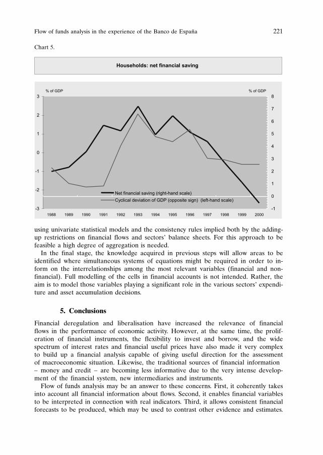
using univariate statistical models and the consistency rules implied both by the adding-up restrictions on financial flows and sectors’ balance sheets. For this approach to befeasible a high degree of aggregation is needed.In the final stage, the knowledge acquired in previous steps will allow areas to beidentified where simultaneous systems of equations might be required in order to in-form on the interrelationships among the most relevant variables (financial and non-financial). Full modelling of the cells in financial accounts is not intended. Rather, theaim is to model those variables playing a significant role in the various sectors’ expendi-ture and asset accumulation decisions.
5. Conclusions
Financial deregulation and liberalisation have increased the relevance of financialflows in the performance of economic activity. However, at the same time, the prolif-eration of financial instruments, the flexibility to invest and borrow, and the widespectrum of interest rates and financial useful prices have also made it very complexto build up a financial analysis capable of giving useful direction for the assessmentof macroeconomic situation. Likewise, the traditional sources of financial information– money and credit – are becoming less informative due to the very intense develop-ment of the financial system, new intermediaries and instruments.Flow of funds analysis may be an answer to these concerns. First, it coherently takesinto account all financial information about flows. Second, it enables financial variablesto be interpreted in connection with real indicators. Third, it allows consistent financialforecasts to be produced, which may be used to contrast other evidence and estimates.
Flow of funds analysis in the experience of the Banco de Espana 221
�
�
�
�
�
�
�
��� ��� �� �� ��� ��� �� ��� ��� ��� ��� ��� �
��
��
�
�
�
��� ��������� ������ ����������� ������
�������� ������� � � !"# � $$ ���� ����� ���������� ������
% � !"#% � !"#
���������� ��� �������� ������
Chart 5.

And finally, this approach helps assess certain features of financial stability by focusingon the sectoral financial situation.Summing up, progress in flow of funds analysis will, in our view, allow financial vari-ables to play a more relevant role in any assessment of the economic situation. Beforethis can be attained, a more thorough understanding of financial flows and their rela-tionship to spending decisions is needed.
References
Alho K. (1991): “Financial Markets and Macroeconomic Policy in the Flow-of-Funds Framework”,the Research Institute of the Finnish Economy.
Brainard W. C. and J. Tobin (1968): “Pitfalls in Financial Model Building”, American EconomicReview, vol. 58 nº 2, May, 99–122.
Banco de Espana (1999a): “Analisis de las magnitudes monetarias dentro de la UEM”, in BoletınEconomico, Banco de Espana, June.
Banco de Espana (1999b): “Quarterly Report of the Spanish Economy” (section 5) in EconomicBulletin, Banco de Espana, April.
Cuenca J. A. and F. Saez (2000): “Evolucion de los flujos de rentas por intereses en Espana entre1995 y 1999”, in Boletın Economico, Banco de Espana, February.
Owen P. D. (1986): “Money, Wealth and Expenditure, Integrated Modelling of Consumption andPortfolio Behaviour”, Cambridge University Press, Cambridge.
Penalosa J. M. (1998): “The Financial Position of Economic Agents and Monetary Policy”, in J. L.Malo de Molina, J. Vinals and F. Gutierrez (eds. for the Research Department of the Banco deEspana) Monetary policy and inflation in Spain, Macmillan Press.
Tobin J. (1980): “Asset Accumulation and Economic Activity”, Yrjo Jahnsson Lectures, Basil Black-well, Oxford.
222 Juan Ma Penalosa and Teresa Sastre

Austria: Martin SchurzMaria Valderrama
Belgium: Annick BruggemanVincent Perilleux
Canada: Dinah MacleanJack Selody
Denmark: Christian Ølgaard
Finland: Antti Ripatti
France: Francoise DrumetzIvan Odonnat
Germany: Gabriele KabelacJulian Reischle
Greece: Dimitris Sideris
Ireland: Jim Nugent
Italy: Eugenio GaiottiAlberto Locarno
Japan: Takeshi Kimura
Luxembourg: Patrick LunnemannSandrine Scheller
Netherlands: Maarten van RooijCees Ullersma
Portugal: Pedro Duarte NevesAna Cristina Leal
Spain: Juan PenalosaTeresa Sastre
Sweden: Hans DillenKerstin Mitlid
List of Participants
Switzerland: Thomas JordanMichel Peytrignet
United Kingdom: Peter AndrewsAndrew Hauser
United States: Richard D. Porter
European Central Bank: Jose Luis EscrivaHans-Joachim Klockers (Chairman)Klaus MasuchHuw PillCaroline Willeke
224 List of Participants