QEDQueen’s Economics Department Working Paper No. 1262

Monetary and Fiscal Policies in a Heterogeneous-AgentEconomy

Hongfei SunQueen‘s University

Department of EconomicsQueen’s University

94 University AvenueKingston, Ontario, Canada

K7L 3N6

3-2011

Monetary and Fiscal Policies

In a Heterogeneous-Agent Economy

Hongfei Sun∗

Queen’s University

January 24, 2012

Abstract

I study the effects of long-run inflation and income taxation in an economy where

households face uninsurable idiosyncratic risks. I construct a tractable competitive

search framework that generates dispersion of prices, income and wealth. I ana-

lytically characterize the stationary equilibrium and the policy effects on individual

choices. Quantitative analysis finds that monetary and fiscal policies have distinctive

effects on macro aggregates, such as output, savings, wealth dispersion, income and

consumption inequalities. There can be a hump-shape relationship between welfare

and the respective policies. Overall, welfare can be maximized by a deviation from

the Friedman rule, paired with distortionary income taxation.

JEL Classification Codes: E0, E4, E5, E6, H2, H3.

Keywords: Competitive Search, Distributional Effect, Monetary and Fiscal Policies.

∗Mail address: Department of Economics, Queen’s University, 94 University Avenue, Kingston, Ontario,Canada, K7L 3N6. E-mail address: hfsun@econ.queensu.ca. I thank Gabriele Camera, Allen Head andShouyong Shi for helpful comments and suggestions. I have also benefited from conversations with seminarand conference participants at Queen’s University, 2011 Midwest Macroeconomic Meetings, 2011 CanadianEconomic Association Meetings and 2011 Society for the Advancement in Economic Theory Meetings. Igratefully acknowledge the financial support from the Social Sciences and Humanities Research Council ofCanada. All errors are my own.

1

1 Introduction

I construct a tractable framework of competitive search that endogenously generates dis-

persion of prices, wealth and income. With this framework, I investigate the effects of

long-run inflation and income taxation on the macroeconomy, as well as the interaction of

the two policies. Wealth and income dispersions prevail in modern economies. In the pres-

ence of such distributions, monetary and fiscal policies are likely to have uneven impacts

on households, generating non-trivial effects on real activities and welfare. To maximize

welfare, policy makers must have a good understanding of the distributional policy effects.

In the case where monetary and fiscal authorities are independent of one another, it is

also important to understand policy interactions. This is particularly relevant given the

context that there have been formulations of central banks and monetary unions, as well

as attempts made to form fiscal unions in recent years.

Despite its importance, it is a challenging task to study both policies in a heterogeneous-

agent environment. This is because the individual decision problem is generally affected

by the endogenous wealth distribution. Solving the model involves handling problems

with large dimensions. Policy analysis further enhances the diffi culty because it entails

computing and comparing equilibrium outcomes in various policy scenarios. Therefore, it

is a rare attempt in the literature to examine the distributional effects of monetary and

fiscal policies simultaneously.

In my model, households and firms can trade in frictionless and frictional goods markets.

The frictional market contains a variety of submarkets and is characterized by competitive

search. Households make tradeoffs between the terms of trade and matching probabilities

when choosing which submarket to participate in. Search is competitive in that both

households and firms take as exogenous the terms of trade and the matching probabilities

across all submarkets. In equilibrium, a submarket that requires a higher payment per

transaction offers a higher quantity of goods per transaction and also a higher probability

for a buyer to be matched for a transaction. Households face uninsurable idiosyncratic

shocks on labor preferences, which lead to diverse decisions on consumption, precautionary

savings, labor supply and trading strategies. In equilibrium there will arise dispersions of

price, income and wealth.

Competitive search is a critical feature of this model because it offers significant tractabil-

ity. Unlike commonly-studied bilateral bargaining in a search environment, here individual

traders cannot affect any of the market specifications, i.e. terms of trade and matching

probabilities, due to the competitive nature of the search process. With given trading spec-

ifications, a household need not consider the amount of money that its potential trading

partner might have, when making its optimal decisions. As a result, the household decision2

problem can be solved without involving the endogenous money distribution, which greatly

reduces the state space and renders the model tractable.

I analytically characterize the stationary equilibrium and the policy effects on individual

decisions. Policies include long-run money growth maintained by lump-sum transfers and

a proportional income tax. The government balances budget and rebates tax revenues in

a lump-sum manner. I numerically examine the policy implications on the macroeconomy.

The key findings are the following: First, both policies can directly affect the intensive

and extensive margins (i.e., the quantity per trade and the trading probability per buyer),

and also indirectly through altering household choices of spending in the frictional market.

Quantitatively, the indirect effects tend to dominate the direct ones. Inflation can stimulate

spending and thus has a positive overall effect on both margins, while income taxation

does the opposite. Overall, inflation increases output and consumption but decreases

precautionary savings. Income taxation has the opposite effects.

Second, the effect of inflation on wealth dispersion depends on the tax regime. The

positive effect tends to dominate at lower tax rates while the negative effect tends to

dominate at higher tax rates. Income taxation decreases wealth dispersion regardless

of the monetary policy. Moreover, inflation decreases income inequality but increases

consumption inequality. Taxation has a positive effect on both income and consumption

inequalities.

Finally, inflation and taxation can respectively have a hump-shape relationship with

welfare. The welfare-improving role of inflation is sensitive to the status of the fiscal policy.

It is important to coordinate the two policies. Welfare can be maximized by a deviation

from the Friedman rule together with distortionary income taxation. When the monetary

and fiscal authorities are independent authorities, a change of policy by one has non-trivial

implications on the optimal policy choice of the other.

This framework is based on Rocheteau and Wright (2005; henceforth RW) and Men-

zio, Shi and Sun (2011; henceforth MSS), the former of which studies competitive search

in an environment follows Lagos and Wright (2005; henceforth LW). The LW structure

features quasi-linear preferences and alternating frictional and frictionless markets. It is a

tractable framework because its equilibrium money distribution is degenerate.1 Neverthe-

less, it does not provide insights on the distributional policy effects. Menzio, Shi and Sun

(2011) construct a tractable monetary environment with non-degenerate money distribu-

tions. Because of competitive search, the model has the feature of block recursivity, which

means that individual decision problems can be solved independently from the endogenous

1Because of its tractability, the unique LW framework has prompted an exploding literature on micro-founded models of money with an emphasis on market frictions. This literature has recently been recognizedas the New Monetarist Economics (Williamson and Wright, 2010a,b).

3

distributions.2 Nevertheless, the framework of MSS abstracts away from money growth.

To analyze policy effects while maintaining model tractability, I construct a model that

combines the key features of LW/RW and MSS. With quasi-linear preferences, access to

frictionless markets and competitive search, the model is block recursive even in the context

of both monetary and fiscal policies.

This paper is closely related to the literature of heterogeneous-agent economies that

study the distributional effect of monetary policy. In these models, money is valued either

because of the cash-in-advance constraint (e.g. Imrohorglu, 1992; Erosa and Ventura, 2002;

Camera and Chien, 2011), or for precautionary purpose (e.g. Akyol, 2004; Wen, 2010;

Dressler, 2011), or due to search frictions (e.g. Molico, 2006; Boel and Camera, 2009; Chiu

and Molico, 2010). In most of these models, agents trade in Walrasian markets. Such

models are not able to generate equilibrium price dispersion. The search model can be a

natural environment to have dispersion of prices, e.g. Molico (2006) and Chiu and Molico

(2010), where agents trade in decentralized markets and bargain bilaterally. In contrast to

search models with bargaining, my model features competitive search, which significantly

improves tractability. Finally, none of the above literature examines the distributional

effects of monetary and fiscal policies simultaneously, which is in contrast the main goal of

my paper.

The rest of this paper is organized as follows. Section 2 describes the physical model

environment. Section 3 characterizes the stationary equilibrium. Section 4 presents ana-

lytical policy effects. Section 5 discusses numerical results. Finally, Section 6 concludes

the paper.

2 A Unified Macroeconomic Framework

2.1 The environment

Time is discrete and continues forever. Each time period consists of two sub-periods. The

economy is populated by a measure one of ex ante identical households. Each household

consists of a worker and a buyer. All households consume general goods in the first sub-

period and special goods in the second sub-period. There are different types of special

goods. Every period a household faces a random preference shock, which determines with

equal probability the type of special goods to consume in the current period. Household

members share income, consumption and labor cost. The preference of a household in a

2The concept of block recursivity was first applied to economics by the seminal work of Shi (2009) onequilibrium wage-tenure contracts. Gonzalez and Shi (2010) and Menzio and Shi (2010a,b; 2011) furtherexamine the functioning of labor markets using the notion of block recursive equilibrium.

4

time period is

U (y, q, l) = U (y) + u (q)− θl, (1)

where y is consumption of general goods, q is consumption of special goods and l is labor

input in a time period. The variable θ measures the random disutility per unit of labor.

It is i.i.d. across households and over time, and is drawn from the probability distribution

F (θ) with support[θ, θ], where 0 < θ < θ < ∞. The value of θ is realized at the

beginning of every period, before any decisions are made. The functions u and U are

twice continuously differentiable and have the usual properties: u′ > 0, U ′ > 0; u′′ < 0,

U ′′ < 0; u (0) = U (0) = u′(∞) = U ′(∞) = 0; and u′ (0) and U ′ (0) being large but finite.

Households discount future with factor β ∈ (0, 1). All goods are perishable across sub-

periods. There is no insurance on idiosyncratic risks. Nor is borrowing or lending feasible

among households. There is a fiat object called money, which is storable without cost.

General goods are traded in competitive and frictionless markets. Special goods are

traded in frictional markets in that trades are decentralized and that buyers and sellers

are randomly matched in pair-wise meetings. Trading frictions are driven by households’

random demand for special goods. There is a measure one of competitive firms. Firms

hire workers from households, who own equal shares of all firms. The labor market is

competitive. Labor is hired at the beginning of a period and is used in production for

both general and special goods. Each firm can organize production of general goods and

one type of special goods. In each period the frictionless goods market opens in the first

sub-period, followed by the frictional market in the second sub-period.3

Trading in a frictional market is characterized by competitive search. This market

contains a variety of submarkets. Each submarket is characterized by (x, q, b, s), where

(x, q) are the terms of trade and (b, s) are the respective matching probabilities for a buyer

and a shop. Search is competitive in the sense that households and firms take as given

the characteristics of all submarkets, when making their trading decisions. Buyers and

shops are randomly matched in a pair-wise manner because households and firms cannot

coordinate. A buyer can enter at most one submarket in each period. Firms have free entry

to all submarkets and choose the measure of shops to operate in each submarket. The cost

of operating a shop for one period is k > 0 units of labor. Moreover, producing q units

of special goods requires ψ (q) units of labor, where ψ is twice continuously differentiable

with the usual properties: ψ′ > 0, ψ′′ ≥ 0 and ψ (0) = 0. In equilibrium free entry of

firms is such that the characteristics of submarkets are consistent with the specified ones.

3In this environment, one can also assume that the frictionless and frictional goods markets opensimultaneously in a period. The results are similar to the sequential order of markets. Here I adopt thesequential structure for expositional convenience.

5

The matching technology has constant returns to scale and is such that s = µ (b). In

equilibrium the matching probabilities of each submarket become functions of the terms

of trade (x, q), as is shown in (4). Therefore, a submarket can be suffi ciently indexed by

(x, q). I impose the following assumption:

Assumption 1 For all b ∈ [0, 1], the matching function µ (b) satisfies: (i) µ (b) ∈ [0, 1],

with µ (0) = 1 and µ(1) = 0, (ii) µ′ (b) < 0, and (iii) [1/µ (b)] is strictly convex, i.e.,

2 (µ′)2 − µµ′′ > 0.

I focus on the steady state equilibrium and suppress the time index throughout the

paper. The per capita money stock is fixed at M for now. I will allow money growth and

income taxation when I analyze policy effects in section 4. Labor is the numeraire. In

particular, let m denote the real value of a household’s money balance measured in terms

of labor units. Let w denote the normalized wage rate, which is the nominal wage rate

divided by the money stock M . Then the dollar amount associated with a balance m is

(wM)m.

2.2 A firm’s decision

In the frictionless market, a representative firm takes the general-good price as given and

chooses output Y to maximize profit. For simplicity, it takes one unit of labor to produce

one unit of general goods. Let p be the price of general goods, measured in terms of labor.

In the frictional market, the firm takes the terms of trade for each submarket, (x, q), as

given and chooses the measure of shops, dN (x, q), to set up in each submarket. Recall

that a shop is matched by a buyer with probability s (x, q). For a particular shop in the

submarket, the operational cost is k units of labor and the expected cost of production is

ψ (q) s (x, q) units of labor. A shop’s expected revenue is xs (x, q), where the revenue x is

measured in labor units. The firm’s total profit in a period is

π = maxY{pY − Y } + max

dN(x,q)

{∫{xs (x, q)− [k + ψ (q) s (x, q)]} dN (x, q)

}. (2)

The first item on the right-hand side denotes the firm’s profit in the frictionless market

and the second item its profit in the frictional market. Free entry of firms implies that the

firm earns zero profit and thus p = 1 in equilibrium. Zero-profit in the frictional market

requires

s (x, q) [x− ψ (q)] ≤ k and dN (x, q) ≥ 0, (3)

where the two inequalities hold with complementary slackness. In particular, if the ex-

pected profit of operating a shop s (x, q) [x− ψ (q)] − k < 0, then the firm will choose6

dN (x, q) = 0. If s (x, q) [x− ψ (q)] − k = 0, the firm is indifferent across any dN (x, q) ∈(0,∞). It is not an equilibrium to have s (x, q) [x− ψ (q)] − k > 0 because it would at-

tract the firm to choose dN (x, q) = ∞, which contradicts zero-profit. As is common inthe competitive search literature,4 I focus on equilibria where condition (3) also holds for

submarkets not visited by any buyer. Given that the trading probabilities b, s ∈ [0, 1],

condition (3) implies

s (x, q) = µ (b (x, q)) =

{k

x−ψ(q), if k < x− ψ (q)

1, if k ≥ x− ψ (q) .(4)

The free-entry condition pins down the matching probabilities in a submarket as functions

of the terms of trade. Indeed, a submarket can be suffi ciently indexed by the terms of

trade, (x, q).

2.3 A household’s decision

2.3.1 Decision in the frictionless market

Let W (m, θ) be a household’s value at the beginning of a period with real money balance

m and the random realization θ. Given price p and the characteristics of all frictional

submarkets, a household maximizes its value by choosing consumption of general goods

y ≥ 0, labor input l ≥ 0, the real balance to spend in the frictional market z ≥ 0, and

precautionary savings h ≥ 0.5 If the household’s buyer is matched with a shop in the

frictional market, then the buyer spends z and the household carries h into the following

period. Otherwise, the household carries a balance z + h into the following period. More-

over, z + h ≤ m, where m is the maximum real money balance that a household can carry

across periods. I assume 0 < m < U ′−1(θ). The dividend Π is paid to the household at

the end of a period. In equilibrium Π = 0 because firms earn zero profit.

4For example, Moen (1997), Acemoglu and Shimer (1999), and Menzio, Shi and Sun (2011). Givensuch beliefs off the equilibrium, markets are complete in the sense that a submarket is inactive only if theexpected revenue of the only shop in the submarket is lower than its expected cost given that some buyersare present in the submarket. Such a restriction can be justified by a “trembling-hand”argument that aninfinitely small measure of buyers appear in every submarket exogenously.

5Without the θ-shock, the household has no incentive to choose h > 0, not even when θ is permanentlyheterogeneous across households. With this preference shock, the household saves (more than any unspentbalance z) in a low-θ state to help ease future disutility of labor. Therefore, the role of the preferenceshock here is not only to generate endogenous distributions but also to induce precautionary savings.

7

The value W (m, θ) satisfies the following Bellman equation:

W (m, θ) = max(y,l,z,h)

{U (y)− θl + V (z, h)} (5)

s.t. py + z + h ≤ m+ l.

The constraint in the above is a budget constraint.6 The function V (z, h) is the household’s

value at the beginning of the second sub-period, i.e., immediately before the frictional

market opens. Because the analysis on the decisions of frictional trading is much involved,

I will postpone fully characterizing V until the next sub-section. In Lemma 3, I show that

V is differentiable and concave in z and h. For now, I take such information as given.

Given U ′ > 0, the budget constraint must hold with equality and thus

l = y + z + h−m, (6)

where I have incorporated the equilibrium price p = 1. For now I assume that the choice

of l is interior, which I will verify later. Using (6) to eliminate l in the objective function

yields

W (m, θ) = θm+ maxy{U (y)− θy}+ max

z,h{V (z, h)− θ (z + h)} . (7)

The optimal choices must satisfy the following first-order conditions:

U ′ (y) ≤ θ, and y ≥ 0 (8)

Vz (z, h)

{≤ θ, and z ≥ 0

≥ θ, and z ≤ m− h,(9)

Vh (z, h)

{≤ θ, and h ≥ 0

≥ θ, and h ≤ m− z(10)

6Note that the household’s spending in the frictional market is not constrained by its initial moneyholdings of the period. This is because in this environment both money and firm IOUs can be used in alltransactions. Firm IOUs take the form of a firm’s promise of wage payments at the end of a period, interms of money. Firm IOUs are settled in a central clearinghouse at the end of a period. Such IOUs areenforceable because firms are large (in the sense that each of them owns a positive measure of shops) andthus they have deterministic revenues and costs, although individual shops face matching risks. Firms lastfor one period and new ones are formed at the beginning of the next. Thus firm IOUs can be circulatedfor only one period. Nevertheless, personal IOUs of households are not accepted as a medium of exchangebecause households face idiosyncratic preference and matching risks and there is no enforcement on theirIOUs. No particular type of goods is cash goods in this environment because both fiat money and firmIOUs can be used in all transactions. This is in contrast with standard money search models, where goodstraded in the frictional markets are considered cash goods. In these models, fiat money must be used as amedium of exchange to overcome the lack of double coincidence of wants and record-keeping of individualtraders.

8

where all sets of inequalities hold with complementary slackness. Given 0 < m < U ′−1(θ),

it follows that

θ ≤ θ < U ′ (m) < U ′ (0)

for all θ ∈[θ, θ]. Then condition (8) implies that the choice of y is always interior and

satisfies

U ′ (y) = θ. (11)

Clearly, the household’s current money balance m does not affect the optimal choices of y,

z or h, although it does affect l. Let the policy functions be y (θ), z (θ), h (θ) and l (m, θ).

Note that z (θ) + h (θ) ≥ 0 for all θ ∈[θ, θ]and that m ≤ m. Therefore, (6) and (11)

imply that l (m, θ) ≥ U ′−1(θ)− m > 0 for all (m, θ). That is, all households’choices of l

are interior given that U ′−1(θ)> m. Given (7), the value function W is

W (m, θ) = W (0, θ) + θm, (12)

where

W (0, θ) = U (y (θ))− θy (θ) + V (z (θ) , h (θ))− θ [z (θ) + h (θ)] .

(13)

The preceding exposition proves the following lemma:

Lemma 1 The value function W is continuous and differentiable in (m, θ). It is also

affi ne in m.

2.3.2 Decision in the frictional market

The household chooses whether to participate in the frictional market. If yes, then it

chooses which submarket to enter and search for a trade. Given balances z and h, the

household is faced with the following problem at the beginning of the second sub-period:

maxx,q{b (x, q) [u(q) + βE [W (z − x+ h, θ)]] + [1− b (x, q)] βE [W (z + h, θ)]} ,

(14)

where q ≥ 0, x ≤ z and b (x, q) is determined by (4). It is convenient to use condition (4)

to eliminate q in the above objective function. Given linearity of W , the problem in (14)

9

simplifies to

maxx≤z, b∈[0,1]

b

{u

(ψ−1

(x− k

µ (b)

))− βE (θ)x

}+ βE [W (z + h, θ)] . (15)

The optimal choices satisfy the following first-order conditions

u′(ψ−1

(x− k

µ(b)

))ψ′(ψ−1

(x− k

µ(b)

)) − βE (θ) ≥ 0, and x ≤ z, (16)

u

(ψ−1

(x− k

µ (b)

))− βE (θ)x+

u′(ψ−1

(x− k

µ(b)

))ψ′(ψ−1

(x− k

µ(b)

)) kbµ′ (b)

[µ (b)]2≤ 0, and b ≥ 0,

(17)

where the two sets of inequalities hold with complementary slackness. It has been taken

into account in condition (17) that b = 1 cannot be an equilibrium outcome. This is

because b = 1 implies s = 0. This further implies that firms choose dN (z, q) = ∞ and

earn strictly positive profit, which violates free entry. Let the policy functions be x (z),

b (z) and q (z), where q (z) is implied by condition (4):

q (z) = ψ−1

(x (z)− k

µ (b (z))

). (18)

If b (z) = 0, then the choices of x and q are irrelevant. In this case, the household chooses

not to participate in the frictional submarket. Without loss of generality, I impose x (z) = z

if b (z) = 0.

Now consider z such that b (z) > 0. It is obvious from (15) that the optimal choices

are independent of z if the money constraint does not bind, i.e., x (z) < z. Define Φ (q) ≡u′ (q) /ψ′ (q). If x (z) < z, then (16) holds with equality. Then conditions (16) and (18)

imply

q∗ = Φ−1 [βE (θ)] . (19)

Given q∗, using (18) to eliminate x in (17) yields

u (q∗)− βE (θ)

[ψ (q∗) +

k

µ (b∗)

]+

[u′ (q∗)

ψ′ (q∗)

]kb∗µ′ (b∗)

[µ (b∗)]2= 0. (20)

It is straightforward to show that the left-hand side of (20) is strictly increasing in b∗.

10

Moreover, b∗ > 0 exists and is unique if E (θ) satisfies

u(Φ−1 [βE (θ)]

)− βE (θ)

[ψ(Φ−1 [βE (θ)]

)+ k]> 0. (21)

Given unique values of q∗ and b∗, x∗ is uniquely determined by

x∗ = ψ (q∗) +k

µ (b∗). (22)

Therefore, if condition (21) holds, then x (z) = z for all z < x∗ and x (z) = x∗ for all

z ≥ x∗. If condition (21) fails to hold, then x (z) = z for all z ≥ 0. Define z as the

maximum value such that x (z) = z. Thus z = x∗ if (21) holds and z =∞ otherwise.

In this environment, it is not necessary for the household to choose z higher than the

amount x that it plans to spend in the frictional market. Without loss of generality, I

impose x (z) = z in the rest of the analysis. In particular, consider z ∈ [0, z]. Given such

z, the problem in (15) becomes

B (z) + βE [W (z + h, θ)] , (23)

where

B (z) = maxb∈[0,1]

b

{u

(ψ−1

(z − k

µ (b)

))− βE (θ) z

}. (24)

The value B (z) is the household’s expected trade surplus. If b > 0, it must be the case

that q > 0 and that the surplus from trade is strictly positive:

u

(ψ−1

(z − k

µ (b)

))− βE (θ) z > 0. (25)

Moreover, the optimal choice of b satisfies condition (17) given x = z.

Lottery choice. It is necessary to mention that the value function B (z) may not be

concave in z because the objective function in (24) may not be jointly concave in its state

and choice variables, (z, b). This objective function involves the product between the choice

variable b itself and a function of b. Even if both of these two terms are concave, the product

may not be jointly concave. Above all, it is unclear whether either of the two terms is a

concave function of z, given that b is a choice variable and is yet to be determined. To make

the household’s value function concave, I introduce lotteries with regards to the balance

z, as in Menzio, Shi and Sun (2011). In particular, lotteries are available every period

immediately before trading in the frictional market takes place.

A lottery is characterized by (L1, L2, π1, π2). If a household plays the lottery, it will11

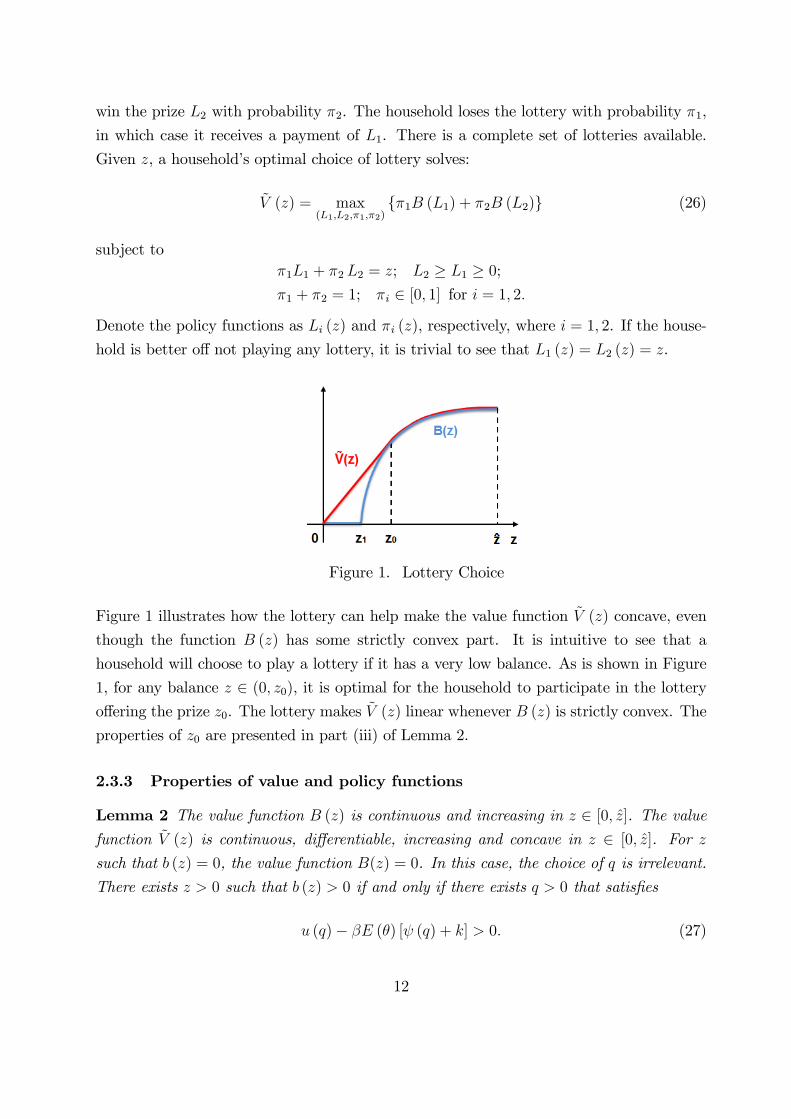
win the prize L2 with probability π2. The household loses the lottery with probability π1,

in which case it receives a payment of L1. There is a complete set of lotteries available.

Given z, a household’s optimal choice of lottery solves:

V (z) = max(L1,L2,π1,π2)

{π1B (L1) + π2B (L2)} (26)

subject toπ1L1 + π2 L2 = z; L2 ≥ L1 ≥ 0;

π1 + π2 = 1; πi ∈ [0, 1] for i = 1, 2.

Denote the policy functions as Li (z) and πi (z), respectively, where i = 1, 2. If the house-

hold is better off not playing any lottery, it is trivial to see that L1 (z) = L2 (z) = z.

Figure 1. Lottery Choice

Figure 1 illustrates how the lottery can help make the value function V (z) concave, even

though the function B (z) has some strictly convex part. It is intuitive to see that a

household will choose to play a lottery if it has a very low balance. As is shown in Figure

1, for any balance z ∈ (0, z0), it is optimal for the household to participate in the lottery

offering the prize z0. The lottery makes V (z) linear whenever B (z) is strictly convex. The

properties of z0 are presented in part (iii) of Lemma 2.

2.3.3 Properties of value and policy functions

Lemma 2 The value function B (z) is continuous and increasing in z ∈ [0, z]. The value

function V (z) is continuous, differentiable, increasing and concave in z ∈ [0, z]. For z

such that b (z) = 0, the value function B(z) = 0. In this case, the choice of q is irrelevant.

There exists z > 0 such that b (z) > 0 if and only if there exists q > 0 that satisfies

u (q)− βE (θ) [ψ (q) + k] > 0. (27)

12

For z such that b (z) > 0, the value function B (z) is differentiable, B(z) > 0 and B′(z) > 0.

Moreover, the following results hold: (i) The policy functions b (z) and q (z) are unique and

strictly increasing in z. In particular, b (z) solves

u (q (z))− βE (θ) z +

[u′ (q (z))

ψ′ (q (z))

]kb (z)µ′ (b (z))

[µ (b (z))]2= 0, (28)

where

q (z) = ψ−1

(z − k

µ (b (z))

). (29)

Moreover, b (z) strictly decreases in E (θ) while q (z) strictly increases in E (θ); (ii) There

exists z1 > k such that b (z) = 0 for all z ∈ [0, z1] and b (z) > 0 for all z ∈ (z1, z]; (iii)

There exists z0 > z1 such that a household with z < z0 will play the lottery with the prize

z0. Moreover, B (z0) = V (z0) > 0, B′ (z0) = V ′ (z0) > 0 and b (z0) > 0.

Lemma 2 (see Appendix A for a proof) summarizes the properties of the household’s

value and policy functions in the frictional market. According to part (i), the optimal

choices of (q, b) are strictly increasing in z when the household chooses b > 0 to participate

in frictional trading. In this case, the higher a balance the household spends, the higher a

quantity it obtains and the higher the matching probability at which it trades. As a result,

households endogenously sort themselves into different submarkets based on their balances

to spend. For any given z, a higher value of E (θ) implies a lower matching probability for

the buyer and a higher amount of goods to be purchased by the buyer. The intuition is the

following: Given higher E (θ), it becomes more costly for firms to hire labor. Firms respond

by setting up fewer shops in a submarket but increasing quantity produced per trade. This

helps save the fixed cost of operating shops and steer more labor into production. All else

equal, more shops in a submarket lead to a higher matching probability for a shop, which

tends to increase a firm’s revenue. Thus the firm can afford to offer a higher quantity per

trade, even though it requires a higher labor input. In this case, households face a lower

matching probability for a buyer. Nevertheless, the households are compensated by an

increase in the quantity per purchase.

Recall that V is the value of a household at the beginning of the second sub-period

before trading decisions are made. Given (12), (23), (24) and (26), V is given by

V (z, h) = V (z) + βE [W (0, θ)] + βE (θ) (z + h) . (30)

Clearly V is linear in h. Recall from (7) that the household chooses z and h to solve the

13

following problem:

maxz,h{V (z, h)− θ (z + h)} . (31)

It follows that h (θ) > 0 if and only if θ is such that V ′ (z (θ)) = 0, that is, if z (θ) = x∗

as defined in (22). In this case, h (θ) = m− x∗. For all θ such that z (θ) < x∗, it must be

that h (θ) = 0. Then (6) implies

l (m, θ) =

{y (θ) + m−m, if z (θ) = x∗

y (θ) + z (θ)−m, if z (θ) < x∗.(32)

Given Lemma 1 and Lemma 2, it is trivial to derive the following lemma:

Lemma 3 (i) V is continuous and differentiable in (z, h). The function V (·, h) is increas-

ing and concave in z ∈ [0, z], with V (z, h) ≥ βE [W (0, θ)] > 0 for all z. Moreover, V (z, ·)is affi ne in h. If θ is such that z (θ) = x∗, then h (θ) = m − x∗. Otherwise, h (θ) = 0;

(ii) Policy functions y (θ), z (θ) and h (θ) are decreasing functions. The policy function

l (m, θ) is decreasing in both m and θ.

3 Stationary Equilibrium

Definition 1 A stationary equilibrium consists of household values (W,B, V , V ) and choices

(y, l, z, h, (q, b) , (L1, L2, π1, π2)); firm choices (Y, dN (x, q)); price p and wage rate w. These

elements satisfy the following requirements: (i) Given the realizations of shocks, asset bal-

ances, prices and terms of trade, a household’s choices solve (7), (24), (26) and (30), which

induce the value functionsW (m, θ), B(z), V (z) and V (z, h); (ii) Given prices and terms of

trade, firms maximize profit and solve (2); (iii) Free entry condition: The function s(x, q)

satisfies (4); (iv) All labor markets, general-good markets and money markets clear; (v)

Stationarity: All quantities, prices and distributions are time invariant; (vi) Symmetry:

Households in the same idiosyncratic state make the same optimal decisions.

The above definition is self-explanatory. The labor-market-clearing condition implies

that the equilibrium normalized wage rate w∗ is determined by

(w∗)−1 =

∫ θ

θ

h (θ) dF (θ) +2∑i=1

∫ θ

θ

πi (z (θ)) [1− b (Li (z (θ)))]Li (z (θ)) dF (θ) . (33)

I derive the above market-clearing condition in Appendix D. Given the equilibrium defin-

ition, I have the following theorem (see Appendix B for a proof):

14

Theorem 2 A stationary equilibrium exists. It is unique if and only if the lottery choices

{L1 (z (θ)) , L2 (z (θ)) , π1 (z (θ)) , π2 (z (θ))} are unique for all z (θ). Moreover, the following

results hold: (i) The general-good consumption y (θ) > 0 for all θ; (ii) If there does not

exist q > 0 that satisfies condition (27), then z (θ) = 0 for all θ. Otherwise, z (θ) > 0 for

some θ.

According to Theorem 2, frictionless markets are always active, while frictional markets

are not. A necessary condition for frictional markets to be used is that condition (27) holds

for some q > 0. This condition depends on the preferences and the production technology

for special goods, the discount factor and the value of E (θ). Intuitively, if the utility

derived from consuming special goods is too low, or if the production cost of special goods

is too high, consumption of special goods can become too costly, especially considering the

uncertainty involved in obtaining such goods. Similarly, if E (θ) is too high, then the cost

of labor is high, which drives up the cost of producing special goods and hence suppresses

the demand. These results are consistent with the findings in Camera (2000). In a model

without distributional components, Camera shows that the frictional market is used in

equilibrium when households can have suffi ciently high expected consumption relative to

that in the frictionless market.

Note that this equilibrium is remarkably tractable. None of the decision problems (7),

(24), (26) and (30) is affected by the endogenous money distribution. Therefore, one can

solve these decision problems first, and then use the household optimal decisions to derive

the equilibrium aggregates, together with income and wealth distributions. This model

property is called block recursivity.

4 Policy Effects

I now analyze the effects of monetary and fiscal policies. Consider that the money stock

per capita evolves according toM ′ = γM , where γ ≥ β is the money growth rate andM ′ is

the money stock of the next period. Money growth is achieved by a lump-sum transfer from

the government to households, and vice versa for money contraction. The government also

imposes a proportional tax rate τ ∈ [0, 1) on wage income. The government balances its

budget every period. All tax revenues are redistributed from the government to households

in a lump-sum manner. Transfers are made at the beginning of each period. All tax

payments and transfers are made with money. The money market opens in the second

subperiod of a period.

First, it is straightforward to show that ∂y (θ) /∂τ ≤ 0 and ∂y (θ) /∂γ = 0. The former

is a standard income effect and the latter is also a standard result in the macro literature.15

Second, policies directly affect equilibrium trading strategies, q (z) and b (z). The effect on

q (z) is called the intensive-margin effect and the one on b (z) the extensive-margin effect.

Even with policies, all the results in Lemma 2 still hold, except that the policy functions

b (z) and q (z) are jointly determined by

u (q (z))− βE (θ)

γ (1− τ)z +

[u′ (q (z))

ψ′ (q (z))

]kb (z)µ′ (b (z))

[µ (b (z))]2= 0 (34)

q (z) = ψ−1

(z − k

µ (b (z))

), (35)

instead of (28) and (29). Then follows a proposition on policy effects (see Appendix C for

a proof):

Proposition 1 For all z such that b (z) > 0, the following results hold:

(i) Given z, fiscal policy τ has a positive direct effect on the intensive margin and a

negative direct effect on the extensive margin, i.e., ∂q(z;τ)∂τ

> 0 and ∂b(z;τ)∂τ

< 0;

(ii) Given z, monetary policy γ has a negative direct effect on the intensive margin and

a positive direct effect on the extensive margin, i.e., ∂q(z;γ)∂γ

< 0 and ∂b(z;γ)∂γ

> 0;

(iii) Fiscal policy has a negative effect on spending z, i.e., ∂z(θ;τ)∂τ

< 0. By decreasing

z (θ), fiscal policy τ has a negative indirect effect on both margins b and q. The effect of

monetary policy on z is ambiguous and hence the indirect effect of monetary policy on both

margins is also ambiguous;

(iv) On the extensive margin, the overall fiscal policy effect is negative. The fiscal policy

effect on the intensive margin is ambiguous given the opposing direct and indirect effects.

Proposition 1 characterizes both direct and indirect policy effects on intensive and

extensive margins, b (z) and q (z). Each policy has a direct impact on the choices of b

and q, as well as an indirect one through affecting the choice of spending z. Part (i)

summarize the direct effects of proportional income taxes. A higher income tax rate τ

makes households frugal on spending. For any given balance, a household chooses to visit

a submarket that offers a higher quantity of goods per trade, which is a positive effect on

the intensive margin. In such a submarket, a firm’s cost of production per trade is higher.

Thus it reduces overall cost by setting up a smaller measure of shops in this submarket.

This imposes a negative effect along the extensive margin.

Part (ii) of Proposition 1 lists the direct monetary policy effects on the margins. In

particular, the real value of a money balance over time decreases with money growth. A

household responds by sending its buyer to a submarket with a higher matching probability

16

b, in order to increase the chance of spending money in the current period. In such a

submarket, the matching probability for a shop is lower, which all else equal implies a

lower profit for firms. Zero profit condition requires that firms must be compensated by

producing a lower quantity per trade. These results of monetary policy are standard and

have been well-documented in the money search literature.

Part (iii) shows that income taxes reduce spending z, which is an income effect. Thus

taxation also has a negative indirect effect on the margins because b and q are increasing

in z. Money growth has an ambiguous effect on z. Intuitively, inflation tax weakens a

household’s incentives for precautionary savings, which causes a positive effect on z as the

household switches some savings (future consumption) to spending on current consumption.

On the other hand, money growth also has a negative effect on z as the household has the

incentives to reduce spending in the frictional market. This is because an unmatched

participation in the frictional market will result in the household carrying the unspent

money balance into the future and bearing the inflation tax. If the household values

consumption of special goods high enough, the first effect dominates and thus inflation can

have a positive indirect effect on both margins by increasing z (θ). The result in part (iv)

is self-explanatory and follows directly from the previous parts.

Finally, it is worthwhile mentioning that all the results in parts (i), (iii) and (iv) of

Proposition 1 are novel analytical results in the current literature on search-theoretic mod-

els of money. The literature has rarely analyzed the effect of fiscal policy on frictional

trading strategies, let alone in a heterogeneous-agent environment.

5 Numerical Results

I now report numerical results on policy effects. I employ the following functional forms:

u(c) =(c+ a)1−σ − a1−σ

1− σ ; U (c) = U0(c+ a)1−σu − a1−σu

1− σu;

ψ(q) = qχ; µ(b) = (1− bρ)1/ρ ; F (θ) is uniform on θ ∈[θ, θ]. (36)

As the benchmark computation, I adopt the following parameter values:

β U0 a σ σu χ k ρ m θ θ γ τ

0.96 20 10−3 1.01 2 1.5 0.01 1 2 0.5 1.5 [β, 2] [0, 0.25](37)

The model period is set to be one year. The discount factor β is chosen to match an annual

interest rate of 4%. For the utility functions, I take σ = 1.01 as a normalization. The value

σu = 2 is typical in the macro literature. The constant a is used to satisfy U(0) = 0. For17

the production function, χ is chosen such that the production function takes the form of

output Q = L2/3 as in a standard RBC model. The cost k is set to a small number. The

matching technology is the so-called telegraph matching function. With ρ = 1, the number

of matches in a submarket with Nb buyers and Ns shops is NbNs/(Nb + Ns). I restrict

my attention to policy parameters γ ∈ [β, 2] and τ ∈ [0, 0.25]. The parameters(m, θ

)are

such that all households θ ≤ θ have interior labor choices under the considered policy

values. This is important for tractability because it allows one to transform the decision

problem (5) into (7). This way, the household’s choices of (y, z, h, q, b, L1, L2, π1, π2) are

independent of the state variable m and also the money distribution. After the benchmark

case, I will also discuss results from variations on the values of(U0, σu, k, ρ, θ, θ

).

Computation strategy. This model is block recursive even with monetary and fiscal

policies. The decision problems are listed in (41)-(44), none of which is affected by equi-

librium distributions. For simulations, one can first solve these problems, and then derive

the equilibrium wage rate, the government transfer and the macro aggregates using the

formulas presented in Appendix D.

Policy functions. Panel A of Figure 2 depicts a household’s optimal lottery choice

given balance z. In particular, z0 = 0.027. That is, any household with z ∈ (0, 0.027) will

play the lottery of receiving either a payment of 0.027 or nothing. For households with

z > 0.027, the functions L1 (z) and L2 (z) almost always coincide, indicating that the lottery

is almost never played at higher z values. Moreover, for the policy parameters considered

here, a household with any θ ∈[θ, θ]never chooses z (θ) ≤ 0.027. Therefore, the lottery

choice is quantitatively negligible in this numerical exercise. For expositional convenience,

I will ignore lotteries when presenting the rest of the numerical results. Nevertheless, all

computation results presented in this paper are carried out with the lottery choice.

Panel B of Figure 2 depicts the policy functions under various policy regimes. In the top

right panel of Figure 2−B, the blue curve coincides with the green curve and is completelyblocked by the latter. In the bottom three panels, all three colored curves are not always

discernible in the graphs because they often coincide with one another. In each panel, a

shift from the blue curve to the red one represents the effect of an increased income tax

rate (from τ = 0 to τ = 0.25) given a money growth rate (γ = 0.96). Similarly, a shift

from the blue curve to the green one represents the effect of an increased money growth

rate (from γ = 0.96 to γ = 1.18) given the fiscal policy (τ = 0). A few observations follow

immediately:

S1. y (θ), z (θ) and h (θ) are decreasing functions, while b (z) and q (z) are increasing

18

functions. This confirms the corresponding results in Lemmas 2 and 3;

S2. (a) Consider a given γ. For any θ, a higher τ decreases z (θ) and y (θ), but increases

savings h (θ). The effect of τ on z is consistent with part (iii) of Proposition 1.

(b) Consider a given τ . Money growth increases the transaction balance z (θ) but

decreases savings h (θ). It has no effect on y (θ). According to part (iii) of Proposition

1, the effect of γ on z can be either positive or negative. Here the numerical results

suggest that the positive effect dominates.

(c) There is equilibrium price dispersion as the equilibrium prices z (θ) /q (z (θ)) vary

with the realizations of θ.

(d) Neither γ nor τ has a significant impact on the functions b (z), q (z) or the price

function z/q (z). This suggests that the direct policy effects summarized in parts

(i)-(ii) of Proposition 1 can be quantitatively small.

The results in S2 are intuitive. All else equal, a higher income tax rate makes it more

costly to supply labor. Accordingly, the household saves more and becomes more frugal on

spending. However, the higher tax rate stimulates precautionary savings because it helps

alleviate the elevated disutility of labor supply in a higher-θ state. Inflation has no effect

on consumption of goods traded in the frictionless market, which is a standard result. All

else equal, inflation tax causes the household to save less yet spend more on goods traded

in the frictional market.

Aggregate margins, output and labor.

S3. Inflation has a positive effect on both of the aggregate intensive and extensive mar-

gins, while the tax rate has a negative effect on them. Inflation increases aggregate

output and labor in the frictional market, while the income taxes decrease such ag-

gregates.

Figure 3 depicts the policy effects on aggregate intensive and extensive margins. The

first column is for the intensive margin, i.e. average quantity per trade in the frictional

market, and the second column is for the extensive margin, i.e. volume of transactions in

the frictional market. The first row shows the monetary policy effect and the second row

is for the fiscal policy. Figure 4 shows the policy effects on aggregate output and labor in

the frictional market. Recall from S2 and Figure 2 that the direct policy effects on the

optimal choices of (b, q) are quantitatively small and are dominated by the indirect policy

effects through z. Since (b, q) are increasing functions of z, a higher γ causes both to rise,19

which further leads to a positive effect on both margins as is shown by Figure 3. The

boost to the margins results in a rise in both output and labor. Finally, the policy effects

on output and labor in the frictionless market are standard. The monetary policy has no

effect on either aggregate and the fiscal policy imposes a negative effect on them. I omit

their numerical characterizations due to limited space.

The positive relationship between inflation and output in the top left panel of Figure

4 is in strong contrast to the results from the previous literature. Typically, a monetary

search model either delivers a negative inflation-output relationship or a hump-shape one.

This is because fiat money is required as a medium of exchange in such models. As a

result, inflation tax eventually will bring down output as inflation gets severe. Similarly,

cash-in-advance models typically find a negative relationship between inflation and out-

put.7 In contrast, here in this model money is used for precautionary purposes rather than

transaction purposes. Households can use money and/or firm credit to buy goods. Infla-

tion causes households to increase their desired trading probabilities and to decrease their

precautionary savings, the latter of which is obvious from the top middle panel in Figure

2 − B. Therefore, at very high inflation rates, precautionary savings go to zero. More-

over, the trading probabilities for a buyer in the frictional market approach one and thus

households carry little unspent money balances over time. Together, the entire economy

functions as if it were a cash-less economy. As a result, output increases with inflation and

stays flat at very high money growth rates. This is consistent with the empirical findings

for the U.S. and some other countries, suggesting a positive long-run relationship between

inflation and output at low inflation rates and little effects at high inflation rates (see King

and Watson, 1992; Bullard and Keating, 1995; McCandless and Weber, 1995; Ahmed and

Rogers, 2000; Rapach, 2003).

Wealth distribution.

S4. Inflation has a negative effect on average wealth while income taxation has a positive

effect on it. The effect of inflation on wealth dispersion depends on the income tax

rate. The positive effect tends to dominate at lower tax rates while the negative

effect tends to dominate at higher tax rates.8 Given money growth, income taxation

reduces wealth dispersion.7Molico (2006) reports a hump-shape relationship between inflation and output in a search environment

with endogenous money distributions. Camera and Chien (2011) find a negative relationship betweeninflation and output in a cash-in-advance environment with endogenous money distributions. Moreover,the negative effect of inflation on output by no means limits to models with heterogeneous agents. It isalso common among monetary models with degenerate money distributions.

8This is in contrast with the results from the theoretical literature that examines the distributionaleffect of monetary policy. For example, in a search-theoretic model with bargaining, Molico (2006) showsthat dispersion in money holdings first decreases and then increases as the inflation rate rises. Moreover,

20

Figure 5 depicts the policy effect of inflation on wealth distribution. Here a household’s

wealth is interpreted as its beginning-of-period real money balances after receiving the

government transfer T given by equation (49). Therefore, the average wealth consists of

aggregate precautionary savings, aggregate unspent balances and the transfer. Recall from

S2 that higher inflation causes households to save less (lower h) and spend more (higher z)

at a higher frequency (higher b). Thus inflation decreases aggregate savings. Its effect on

aggregate unspent balances can be ambiguous. On one hand, households plan on spending

more, which means the level of unspent balances held by a household is also higher. On the

other hand, households also choose to trade with a higher probability, which reduces the

chance of holding an unspent balance across periods. The government transfer includes the

monetary component to achieve money growth and the fiscal component from taxation on

labor income. Both components increase with inflation. The former is because of money

injection and the latter is because aggregate labor increases as inflation rises. Overall,

the negative effect of inflation dominates, which indicates that the negative impact of

inflation on precautionary savings is the dominating force. Now consider the positive

relationship between income taxation and average wealth. Recall from S2 that taxation

makes households save more (higher h) and spend less (lower z) at a lower frequency (lower

b). Moreover, higher tax rates reduce aggregate labor and thus the fiscal component of

government transfers. Altogether, the positive effect of income taxation dominates, which

again is likely to the result of the dominating effect on precautionary savings.

Now consider the policy effects on the coeffi cient of variation of wealth. Since all

households receive the same amount of transfers, wealth dispersion critically depends on

the dispersion of precautionary savings and unspent balances. A rise in inflation tends to

increase dispersion in household unspent balances (due to trading frictions) but decrease

dispersion in household savings, which is suggested to a certain extent in Figure 2 by the

changes in the functions z (θ) and h (θ) under various policy regimes. Nevertheless, as the

tax rate rises, households increase savings, which allows the effect of inflation on savings

to make a stronger presence. As is shown by the top right panel of Figure 5, the positive

effect of inflation on dispersion in household unspent balances tends to dominate when the

tax rate is low (e.g. τ = 0). Then at higher tax rates, the negative effect on savings tends

to dominate. In contrast, income taxation unambiguously decreases wealth dispersion.

Chiu and Molico (2010) establish a negative relationship between inflation and the dispersion of themoney distribution. In a model where heterogeneous agents use money to self-insure against liquidityshocks, Dressler (2011) demonstrates that inflation increases dispersion in money balances. In a cash-in-advance environment with heterogeneous agents, Camera and Chien (2011) show that inflation reduceswealth dispersion when money is the only asset, but has little effect on wealth inequality when bonds areintroduced. Moreover, none of the above papers consider the relevance of a fiscal policy regime.

21

Income and consumption inequalities.

S5. Inflation has a negative effect on income inequality but a positive effect on consump-

tion inequality.9 Income taxation has a positive effect on both income inequality and

consumption inequality.

Figure 6 reports policy effects on the respective coeffi cients of variation of household

disposable income and consumption. Inflation reduces income inequality because of the

redistributive effect of lump-sum transfers to sustain money growth. This negative effect

strengthens with higher taxes because income taxation suppresses the incentives to supply

labor. This accentuates the redistributive effect of inflation. Inflation increases consump-

tion inequality because it stimulates participation in the frictional market. Income taxation

increases income inequality. One interpretation is that the negative impact of taxation on

aggregate labor income overpowers its effect on the standard deviation of income. Income

taxation has a positive effect on consumption inequality, which is likely to be related to its

influence on income inequality.

Welfare.

S6. There can be a hump-shape relationship between inflation and welfare at a given tax

rate. The welfare-improving role of inflation strengthens as the tax rate increases.

Similarly, there is a hump-shape relationship between income taxation and welfare

at a given inflation rate.

Figure 7 illustrates the welfare effects. Welfare is defined as the weighted average of the

life-time discounted value W given by (7). Inflation has a positive welfare effect through

the following channels: increasing output, reducing income inequality, and reducing wealth

inequality at higher tax rates. On the other hand, inflation also has a negative welfare

effects by reducing savings, increasing consumption inequality and increasing wealth dis-

persion at lower tax rates. Overall, at a given tax rate, inflation can improve welfare at

lower money growth rates but reduce welfare at higher rates. The higher the tax rate,

the more prominent the positive effect of inflation on welfare. Income taxation also has

both positive and negative impacts on welfare. The positive welfare effect of taxation

comes through increasing savings and decreasing wealth inequality. The negative effect of

9Camera and Chien (2011) also show that inflation lowers income inequality. Nevertheless, there is noconsensus in the empirical literature relating inflation to income distribution. Galli and Hoeven (2001)provide an extensive review over this literature and refer to the mixed results as the “inflation-inequalitypuzzle”. Also in Camera and Chien (2011), lower inflation can increase consumption inequality whenagents are not allowed to borrow.

22

taxation includes decreasing output and increasing income and consumption inequalities.

Altogether, at a given inflation rate, income taxation can also improve welfare at lower tax

rates but end up reducing it at higher tax rates.

The results in S1-S6 are robust to variation of parameter values satisfying the restriction

that the labor choices of all households are strictly positive. For the sake of limited space,

I only report in Table 1 the optimal monetary and fiscal policies under various parameter

values. The benchmark case is given in (37). For each of the other cases, only the parameter

value(s) different from the benchmark case is(are) listed. In the benchmark, the optimal

policy regime is γ∗ = 0.98 and τ ∗ = 0.1. The optimal policy seems very sensitive to

changes in the variability of the θ-shock. Recall θ = 0.5 and θ = 1.5 in the benchmark.

All else equal and keeping E (θ) = 1 constant, the optimal policy goes from γ∗ = 0.96

and τ ∗ = 0.03 given θ ∈ [0.8, 1.2], to γ∗ = 1.01 and τ ∗ = 0.17 given θ ∈ [0.3, 1.7], and to

γ∗ = 1.03 and τ ∗ = 0.22 given θ ∈ [0.2, 1.8]. Since inflation has no effect on real activities

in the frictionless market whatsoever, all of the non-trivial effects of long-run inflation

summarized in S1-S6 are due to trading frictions. This suggests that the trading frictions

can play an important role in reconciling empirical observations on the macroeconomy.

It is clear that monetary and fiscal policies often have opposite yet asymmetric effects

on macro aggregates. Money growth directly affects the intertemporal consumption choices

while income taxation directly affects labor choices across idiosyncratic states. To maximize

welfare, a policy maker must choose the policy pair such that they optimally augment each

other’s positive welfare effects. If the monetary and fiscal authorities are independent of

each other, a policy change by one often implies that the other should adjust its policy

accordingly. For example, in the benchmark case, the optimal money growth rate is γ∗ =

0.96 given τ = 0, γ∗ = 0.98 given τ = 0.1, and γ∗ = 1 given τ = 0.25.

6 Conclusion

I have constructed a tractable framework of competitive search that endogenously gener-

ates dispersion of prices, income and wealth. This model is used to study the implications

of monetary and fiscal policies in an environment with heterogeneous agents. With com-

petitive search, a household’s decision problems can be solved independently from the

endogenous wealth distribution, which brings the model significant tractability. Analytical

and quantitative results suggest that monetary and fiscal policies have distinctive effects

on real activities and welfare. Welfare-maximization requires an optimal policy mix. If

the monetary and fiscal authorities are separate identities, a change of policy by one has a

non-trivial implication on the optimal policy choice of the other.

23

Appendix

A Proof of Lemma 2

Given (24), it is straightforward to see that the value function B (z) is continuous. More-

over, B (z) ≥ 0 for all z ≥ 0, where the equality holds if and only if b = 0. If b = 0, the

choice of q is irrelevant. Since B is continuous on a closed interval [0, z], the lotteries in

(30) make V concave (see Appendix F in Menzio and Shi, 2010b, for a proof). I prove

differentiability of V in the proof of part (iii).

For part (i), define the left-hand side of (17) as LHS (b) and impose x = z:

LHS (b) ≡ u (q)− βE (θ) z +

[u′ (q)

ψ′ (q)

]kbµ′ (b)

[µ (b)]2, (38)

where q is given by (18) with x = z. It is straightforward to derive that

LHS (b = 0) = u(ψ−1 (z − k)

)− βE (θ) z,

= u (q)− βE (θ) [ψ (q) + k] ,

where (18) yields q = ψ−1 (z − k) given b = 0. Thus the above implies that LHS (b = 0) >

0 if and only if there exists q > 0 such that condition (27) holds. Moreover, one can further

derive LHS (b = 1) = −∞, and

LHS ′ (b) = u′ (q) q′ (b) +u′′ (q)ψ′ (q)− u′ (q)ψ′′ (q)

[ψ′ (q)]2 q′ (b)

(kbµ′ (b)

[µ (b)]2

)+ k

[u′ (q)

ψ′ (q)

]µ (b) [µ′ (b) + bµ′′ (b)]− 2b [µ′ (b)]2

[µ (b)]3< 0.

Given all the above results, condition (27) implies that there exists z > 0 such that b > 0.

Furthermore, the above results imply that the policy function b (z) is unique, which further

implies that q (z) is also unique given (18). Given x = z, (16) implies

u′ (q)

ψ′ (q)− βE (θ) > 0. (39)

Therefore, for z such that b > 0,

∂LHS (b; z)

∂z=u′ (q)

ψ′ (q)− βE (θ) +

kbµ′ (b) [u′′ (q)ψ′ (q)− u′ (q)ψ′′ (q)][µ (b)]2 [ψ′ (q)]

3 > 0. (40)

24

This implies that an increase of z shifts the entire function LHS (b) upwards. Because

LHS ′ (b) < 0, it follows that b′ (z) > 0 for all z such that b > 0. Given b > 0, (17) holds

with equality. Total differentiating (17) by z yields

0 = u′ (q) q′ (z)− βE (θ) +kbµ′ (b) [u′′ (q)ψ′ (q)− u′ (q)ψ′′ (q)]

[µ (b)]2 [ψ′ (q)]3 q′ (z)

+ ku′ (q)

ψ′ (q)

[µ (b) [µ′ (b) + bµ′′ (b)]− 2b [µ′ (b)]2

[µ (b)]3

]b′ (z) .

Given b′ (z) > 0 and Assumption 1, rearranging the above yields q′ (z) > 0 for all z such

that b > 0. Given b > 0, one can derive that

B′ (z) = b′ (z) [u (q (z))− βE (θ) z] + b (z)

[u′ (q (z))

ψ′ (q (z))− βE (θ)

]> 0.

This is because b′ (z) > 0 and the trade surplus, u (q (z)) − βzE (θ), is strictly positive

given b > 0, and also condition (39). Obviously, b (z) is strictly decreasing in E (θ), given

the results about LHS (b) in part (ii). Then (29) implies that q (z) is strictly increasing in

E (θ).

For part (ii), note that the previous proof has established that b (z) is continuous and

increasing in all z ∈ [0, z]. In particular, b (z) is strictly increasing in z if b > 0. It is

obvious from (18) that b (z) = 0 for all z ∈ [0, k]. Continuity of b (z) implies that there

exists z1 > k such that b (z) = 0 for all z ∈ [0, z1] and b (z) > 0 for all z > z1.

I now prove part (iii) and the differentiability of V together. If b (z) = 0 for all z,

then obviously V (z) is differentiable. Now consider the case where there exists z such that

b (z) > 0, i.e., condition (27) holds. It is obvious that B (z) is differentiable for all z such

that b (z) > 0. Consider z such that b (z) > 0. Recall that a concave function has both left-

hand and right-hand derivatives (see Royden, 1988, pp113-114). Let V ′ (z−) and V ′ (z+) be

the left-hand and right-hand derivatives, respectively. Suppose V ′ (z−) > V ′ (z+) for some

z such that b (z) > 0. Then V is strictly concave at such z, which implies V (z) = B (z). It

follows that B′ (z−) ≥ V ′ (z−) > V ′ (z+) ≥ B′ (z+), where the first and the last inequalities

follow from the construction of lotteries. However, B′ (z−) > B′ (z+) contradicts the

differentiability of B. Therefore, the value function V (z) is differentiable for all z such

that b (z) > 0. Part (ii) has established that there exists z1 > k such that b (z) = 0 for

all z ∈ [0, z1] and b (z) > 0 for all z > z1. This has two implications: First, B′(z−1)

= 0

because b (z) = B (z) = 0 all z ∈ [0, z1]. Second, B′(z+

1

)> 0 because b (z) > 0 in the right

neighborhood of z1. Therefore, B is strictly convex but not differentiable at z1 because

0 = B′ (z−) < B′ (z+). Strict convexity of B at z1 implies that there is a lottery over the

25

region z ∈ [0, z1]. Let the winning prize of this lottery be z0. Then all households with

z ∈ (0, z0) will play this lottery and receive zero payment if they lose. Moreover, it must

be the case that z0 > z1, b (z0) > b (z1) > 0 and B (z0) = V (z0) > 0. Given b (z0) > 0,

both value functions are differentiable at z0 and B′ (z0) = V ′ (z0) > 0. Therefore, V is

differentiable for all z ∈ [0, z0] because of the lottery. Moreover, V is also differentiable for

all z > z0 because b > 0 for all z > z0. QED

B Proof of Theorem 2

Recall the normalized wage rate w∗ as given in (33). Note that all the policy functions on

the right-hand side of (33) are independent of w∗. Thus w∗ > 0 obviously exists. It follows

that a stationary equilibrium exists and is characterized by w∗. It is unique if and only if

the lottery choices {L1 (z (θ)) , L2 (z (θ)) , π1 (z (θ)) , π2 (z (θ))} are unique for all z (θ). Part

(i) follows from (11). For part (ii), recall from Lemma 2 that there exists z > 0 such that

the policy function b (z) > 0 if any only if condition (27) holds for some q > 0. Therefore,

if (27) does not hold, then b (z) = 0 for all z. Moreover, B(z) = B′(z) = V (z) = V ′(z) = 0

for all z. In this case, the household never trades in the frictional market, which renders no

need to hold a positive balance for transaction purposes. Thus z (θ) = 0 for all θ. Consider

the case where condition (27) holds for some q > 0. In this case, there exists z > 0 such

that the policy function b (z) > 0, according to Lemma 2. Note that condition (9) implies

that z (θ) > 0 if Vz (0, h) ≥ θ. If Vz (0, h) < θ, then z (θ) = 0 is optimal. If z (θ) > 0,

b (L2 (z (θ))) > 0 follows from construction of the lottery. QED

C Proof of Proposition 1

Given policies γ and τ , the household’s decision problem is given by:

W (m, θ) = max(y,l,z,h)

{U (y)− θl + V (z, h)}

s.t. y + z + h ≤ m+ (1− τ) l + T.

Given interior choice of l, the above reduces to

W (m, θ) =θ (m+ T )

1− τ + maxy

{U (y)− θy

1− τ

}+ max

z,h

{V (z, h)− θ (z + h)

1− τ

}. (41)

Moreover,

V (z, h) = V (z) + βE [W (0, θ)] +βE (θ)

γ (1− τ)(z + h) (42)

26

V (z) = max(L1,L2,π1,π2)

{π1B (L1) + π2B (L2)} (43)

s.t. π1L1 + π2 L2 = z; L2 ≥ L1 ≥ 0;

π1 + π2 = 1; πi ∈ [0, 1] for i = 1, 2

B (z) = maxb∈[0,1]

b

{u

(ψ−1

(z − k

µ (b)

))− βE (θ)

γ (1− τ)z

}. (44)

It follows immediately that policy functions b (z) and q (z) are given by (34) and (35).

Define the left-hand side of (34) as

LHSP (b) ≡ u (q)− βE (θ)

γ (1− τ)z +

(u′ (q)

ψ′ (q)

)kbµ′ (b)

[µ (b)]2, (45)

where q is given by (35). Following the same procedure as the proof of Lemma 2, one can

show that Lemma 2 also applies to this case with policies γ and τ , except that condition

(27) is replaced by

u (q)− βE (θ)

γ (1− τ)[ψ (q) + k] > 0, (46)

and (28) and (29) replaced by (34) and (35). As is the case with LHS ′ (b) < 0, we have

LHSP ′ (b) < 0. Then parts (i) and (ii) of this proposition follow trivially given b > 0.

For part (iii), to analyze policy effects on z, note from (41), (42), (43) and (44) that

the decision involving z is given by

maxz

{V (z) +

βE (θ) /γ − θ1− τ z

}.

It is clear from part (ii) of Lemma 2 that b (z) > 0 implies z > 0. Consider interior choice

of z < m, which satisfies the following first-order condition:

V ′ (z) +βE (θ) /γ − θ

1− τ = 0.

Given the lottery, if V (z) is strictly concave at z, then V (z) = B (z) and V ′ (z) = B′ (z).

Moreover, the optimal choice of z satisfies

B′ (z) +βE (θ) /γ − θ

1− τ = 0.

That is,

b

u′(ψ−1

(z − k

µ(b)

))ψ′(ψ−1

(z − k

µ(b)

)) − βE (θ)

γ (1− τ)

+βE (θ) /γ − θ

1− τ = 0. (47)

27

If V (z) is linear at z, then a lottery is employed at z. In this case, V ′ (z) is trivially

determined by the slopes of V at the lottery prize points, L1 (z) and L2 (z). At both of

these points, V (z) is strictly concave. Without loss of generality, I focus on z such that

(47) holds and B′′ (z) < 0.

For the fiscal policy effect, total differentiating (47) yields

0 = B′′ (z) dz +

[u′ (q)

ψ′ (q)− βE (θ)

γ (1− τ)+kbµ′ (b) [u′′ (q)ψ′ (q)− u′ (q)ψ′′ (q)]

[µ (b)]2 [ψ′ (q)]3

]∂b (z; τ)

∂τdτ

+(1− b) βE (θ) /γ − θ

(1− τ)2 dτ . (48)

Similar to (39) and (40), one can show that

u′ (q)

ψ′ (q)− βE (θ)

γ (1− τ)> 0

and that the term within the square bracket of (48) is strictly positive. Then (??) impliesthat θ > βE (θ) /γ > (1− b) βE (θ) /γ. Moreover, we have ∂b

∂τ< 0 according to part (i) of

this proposition. Given B′′ (z) < 0, the above equation implies that dzdτ< 0 given θ. That

is, ∂z(θ;τ)∂τ

> 0.

For the monetary policy effect, total differentiate (47):

0 = B′′ (z) dz +

[u′ (q)

ψ′ (q)− βE (θ)

γ (1− τ)+kbµ′ (b) [u′′ (q)ψ′ (q)− u′ (q)ψ′′ (q)]

[µ (b)]2 [ψ′ (q)]3

]∂b (z; γ)

∂γdγ

− (1− b) βE (θ)

(1− τ) γ2dγ.

where q = ψ−1 (z − k/µ (b)). Again, the term within the square bracket is strictly positive.

Moreover, we have ∂b∂γ> 0 according to part (ii) of this proposition. Given B′′ (z) < 0, the

above equation implies that dzdγ> 0 if[

u′ (q)

ψ′ (q)− βE (θ)

γ (1− τ)+kbµ′ (b) [u′′ (q)ψ′ (q)− u′ (q)ψ′′ (q)]

[µ (b)]2 [ψ′ (q)]3

]∂b (z; γ)

∂γ− (1− b) βE (θ)

(1− τ) γ2> 0.

The above part (iii) shows that z is strictly decreasing in τ . Moreover, part (i) of

Lemma 2 that the policy functions b (z) and q (z) are strictly increasing in z. Thus, the

fiscal policy has a negative indirect effect on both margins through its effect on z. The

28

overall effect of τ is given by

db

dτ=∂b (z (θ; τ) ; τ)

∂τ+ b′ (z)

∂z (θ; τ)

∂τ< 0

because ∂b(z;τ)∂τ

< 0, b′ (z) > 0 and ∂z(θ;τ)∂τ

< 0 for all z such that b (z) > 0. Then rest of the

results in this proposition follow trivially. QED

D Government Transfers and Market Clearing

In this Appendix, I further characterize the market-clearing conditions and the formula for

the government transfer. The analysis in this Appendix is carried out with the monetary

and fiscal policies. For the benchmark case without any policy, one can simply apply γ = 1

and τ = 0 to all the derivations in what follows.

With policies, the definition of a stationary equilibrium must satisfy one more condi-

tion that the government balances its budget every period. For money growth, the house-

hold receives a dollar amount of (γ − 1)M , which is equivalent to (γ − 1)M/ (wM ′) =

(γ − 1) / (wγ) units of labor. For income taxation, the amount of the government transfer

in terms of labor units is τLS. Altogether, the total real transfer received by a household

is given by

T ∗ =γ − 1

w∗γ+τ

γLS. (49)

The market-clearing condition for the general-good market is

Y =

∫ θ

θ

y (θ) dF (θ) . (50)

The market-clearing condition for the labor market is aggregate demand for labor, LD,

is equal to aggregate supply of labor, LS. Consider LD first. A household’s realization

of θ determines the money balance z (θ). Given this money balance, the resulted money

balance after lotteries is Li (z (θ)), i = 1, 2, which takes place with probability πi (z (θ)).

Thus the measure of such households is Nb (θ, i) = πi (z (θ)) dF (θ). The measure of shops

corresponding to the households holding Li (z (θ)) is given by

Ns (θ, i) = πi (z (θ)) dF (θ) b (Li (z (θ))) / [µ (b (Li (z (θ))))] ,

which is derived from b/µ (b) = Ns/Nb given the constant-return-to-scale matching tech-

nology. Then for each shop, the expected labor demand is k + ψ (q)µ (b), which is used to

29

compute the aggregate demand for labor in the frictional market. Thus, LD is given by

LD = Y +2∑i=1

∫ θ

θ

πi (z (θ)) b (Li (z (θ)))

µ (b (Li (z (θ))))[k + ψ (q (Li (z (θ))))µ (b (Li (z (θ))))] dF (θ) .

(51)

The firm’s zero-profit condition (3) implies that for i = 1, 2,

k + ψ (q (Li (z (θ))))µ (b (Li (z (θ)))) = Li (z (θ))µ (b (Li (z (θ)))) .

Then (51) can be transformed to

LD =

∫ θ

θ

y (θ) dF (θ) +2∑i=1

∫ θ

θ

πi (z (θ)) b (Li (z (θ)))Li (z (θ)) dF (θ) . (52)

The aggregate labor supply is given by

LS =

∫ θ

θ

∫l (m, θ) dGa (m) dF (θ) ,

where Ga (m) is the money distribution at the beginning of a period. Given l (m, θ) from

(32),

LS =

∫ θ

θ

∫1

1− τ [py (θ) + z (θ) + h (θ)−m− T ∗] dF (θ) dGa (m) .

Use (49) to substitute for T ∗ in the above. Also recall the constraint for the household’s

lottery choice, π1 (z (θ))L1 (z (θ)) + π2 (z (θ))L2 (z (θ)) = z (θ). It follows that(1− τ +

τ

γ

)LS =

∫ θ

θ

[y (θ) + h (θ) + z (θ)] dF (θ)−∫mdGa (m)− γ − 1

w∗γ. (53)

The household’s beginning-of-the-period balance m consists of precautionary savings and

if any, the transactional balance unspent due to matching frictions. Thus,

∫mdGa (m) =

∫ θ

θ

h (θ)

γdF (θ) +

2∑i=1

∫ θ

θ

πi (z (θ)) [1− b (Li (z (θ)))]Li (z (θ))

γdF (θ) .

(54)

The labor-market clearing requires LD = LS. Thus (52)-(54) together solve for the nor-

30

malized wage rate in the steady state:

(w∗)−1 =

∫ θ

θ

[h (θ) + τy (θ)] dF (θ) + τ2∑i=1

∫ θ

θ

πi (z (θ)) b (Li (z (θ)))Li (z (θ)) dF (θ)

+

2∑i=1

∫ θ

θ

πi (z (θ)) [1− b (Li (z (θ)))]Li (z (θ)) dF (θ) . (55)

Note that the formula in (33) is clearly given by setting τ = 0 in the above equation. Given

that the labor market clears, the money market clears by Walras’law.

31

Figure 2. Policy functions

A. The lottery choice

0 0.2 0.4 0.6 0.8 1 1.2 1.4 1.6 1.8 20

0.2

0.4

0.6

0.8

1

1.2

1.4

1.6

1.8

2

L1(z) and L

2(z)

L1(z)

L2(z)

B. Optimal choices under various policy regimes

0.5 1 1.50.5

0.6

0.7

0.8

0.9

1

1.1

1.2z(theta)

0.5 1 1.50

0.2

0.4

0.6

0.8

1

1.2

1.4h(theta)

0.5 1 1.53

3.5

4

4.5

5

5.5

6

6.5y(theta)

0 0.5 1 1.5 20

0.2

0.4

0.6

0.8

1b(z)

0 0.5 1 1.5 20

0.2

0.4

0.6

0.8

1

1.2

1.4q(z)

0 0.5 1 1.5 20.5

1

1.5

2

2.5

3z/q(z)

gamma=0.96, tau=0

gamma=0.96, tau=0.25gamma=1.18, tau=0

32

Figure 3. Aggregate intensive and extensive margins

A. Average quantity per trade B. Volume of transactions

Figure 4. Output and labor and in the frictional market

A. output B. labor

33

Figure 5. Wealth distribution

A. Average wealth B. Coeffi cient of variation of wealth

Figure 6. Income and consumption inequalities

A. Income inequality B. Consumption inequality

34

Figure 7. Welfare

Table 1. Optimal policy

Parameters γ∗ τ ∗ Parameters γ∗ τ ∗

benchmark 0.98 0.1 σu = 0.5 0.99 0.18

k = 10−3 0.97 0.1 U0 = 12 0.99 0.11

k = 0.5 1 0.07 U0 = 100 0.98 0.07

ρ = 0.5 0.98 0.08 θ ∈ [0.8, 1.2] 0.96 0.03

ρ = 1.5 0.98 0.1 θ ∈ [0.3, 1.7] 1.01 0.17

σu = 1.01 0.98 0.1 θ ∈ [0.2, 1.8] 1.03 0.22

35

References

[1] Acemoglu, D. and R. Shimer, 1999. “Effi cient Unemployment Insurance,”Journal ofPolitical Economy 107, 893-928.

[2] Akyol, A., 2004. “Optimal monetary policy in an economy with incomplete marketsand idiosyncratic risk,”Journal of Monetary Economics 51, 1245-1269.

[3] Boel, P. and G. Camera, 2009. “Financial sophistication and the distribution of thewelfare cost of inflation,”Journal of Monetary Economics 56, 968-978.

[4] Camera, G., 2000. “Money, Search and Costly Matchmaking,”Macroeconomic Dy-namics 4, 289-323.

[5] Camera, G. and Y. Chien, 2011. “Understanding the Distributional Impact of Infla-tion,”Purdue University.

[6] Chiu, J. and M. Molico, 2010. “Liquidity, redistribution, and the welfare cost of infla-tion,”Journal of Monetary Economics 57, 428-438.

[7] Dressler, S., 2011. “Money Holdings, Inflation, and Welfare in a Competitive Market,”International Economic Review 52, 407-423.

[8] Erosa, A. and G. Ventura, 2002. “On Inflation as a Regressive Consumption Tax,”Journal of Monetary Economics 49, 761-795.

[9] Galli, R. and R. Hoeven, 2001. “Is inflation bad for income inequality: The importanceof the initial rate of inflation,”Working Paper, the University of Lugano, Switzerland.

[10] Gonzalez, F. M. and S. Shi, 2010. “An Equilibrium Theory of Learning, Search andWages,”Econometrica 78, 509-537.

[11] Imrohoroglu, A., 1992. “The welfare cost of inflation with imperfect insurance,”Jour-nal of Economics Dynamics and Control 16, 79-91.

[12] Kiyotaki, N. and R. Wright, 1993. “A Search-Theoretic Approach to Monetary Eco-nomics,”American Economic Review 83, 63-77.

[13] Lagos, R. and R. Wright, 2005. “A Unified Framework for Monetary Theory andPolicy Analysis,”Journal of Political Economy 113, 463-484.

[14] Menzio, G. and S. Shi, 2010a. “Directed Search on the Job, Heterogeneity, and Ag-gregate Fluctuations,”American Economic Review: Papers and Proceedings 100.

[15] Menzio, G. and S. Shi, 2010b. “Block Recursive Equilibria for Stochastic Models ofSearch on the Job,”Journal of Economic Theory 145, 1453-1494.

36

[16] Menzio, G. and S. Shi, 2011. “Effi cient Search on the Job and the Business Cycle,”Journal of Political Economy 119, 468-510.

[17] Menzio, G., S. Shi and H. Sun, 2011. “A Monetary Theory with Non-DegenerateDistributions,”University of Toronto Working Paper 425.

[18] Moen, E., 1997. “Competitive Search Equilibrium,”Journal of Political Economy 105,694-723.

[19] Molico, M., 2006. “The Distribution Of Money And Prices In Search Equilibrium,”International Economic Review 47, 701-722.

[20] Rocheteau, G. and R. Wright, 2005. “Money in Search Equilibrium, in CompetitiveEquilibrium, and in Competitive Search Equilibrium,”Econometrica 73, 175-202.

[21] Royden, H. L., 1988. “Real Analysis.”New York: Macmillan.

[22] Shi, S., 2009. “Directed Search for Equilibrium Wage-Tenure Contracts,”Economet-rica 77, 561-584.

[23] Wen, Yi, 2010. “Liquidity Demand and Welfare in a Heterogeneous-Agent Economy,”manuscript, Federal Reserve Bank of St. Louis.

[24] Williamson, S. and R. Wright, 2010a. “New Monetarist Economics: Models,” forth-coming in Benjamin Friedman and Michael Woodford, eds., Handbook of MonetaryEconomics 3A, Second Edition.

[25] Williamson, S. and R. Wright, 2010b. “NewMonetarist Economics: Methods,”FederalReserve Bank of St. Louis Review 92(4), 265-302.

37