Monetary Policy and Distribution

Stephen D. Williamson

Department of Economics

University of Iowa

Iowa City, IA 52242

stephen-williamson@uiowa.edu

http://www.biz.uiowa.edu/faculty/swilliamson

February 2005

Abstract

Amonetary model of heterogeneous households is constructed which deals in

a tractable way with the distribution of money balances across the population.

Only some households are on the receiving end of a money injection from the

central bank, and this in general produces price dispersion across markets.

This price dispersion generates uninsured consumption risk which is important

in determining the effects of money growth, optimal policy, and the effects of

money growth shocks. The optimal money growth rate can be very close to

zero, and the welfare cost of small inßations can be very large. Small money

shocks can have important sectoral effects with small effects on aggregates,

while large money shocks can have proportionately large effects on aggregates.

1

1. INTRODUCTION

The purpose of this paper is to construct a tractable model that takes seriously the

idea that the distributional effects of monetary policy are important for macroeco-

nomic activity. We explore the qualitative and quantitative implications of this model

for the effects of monetary policy on prices, output, consumption, and employment.

Models with distributional effects of monetary policy are certainly not new. The

Þrst models of this type were the limited participation models constructed by Gross-

man and Weiss (1983) and Rotemberg (1984), in which there are always some eco-

nomic agents who are not participating in Þnancial markets and will not be on the

receiving end of an open market operation, at least on the Þrst round. In a limited

participation model, a monetary injection by the central bank causes a redistribution

of wealth which will in general cause short run changes in asset prices, employment,

output, and the distribution of consumption across the population. The subsequent

literature has to a large extent focussed on asset pricing implications, particularly Lu-

cas (1990), Alvarez and Atkeson (1997), and Alvarez, Atkeson, and Kehoe (2002), in

models that, for tractability, Þnesse some of the potentially interesting distributional

implications of monetary policy.

Recent research in monetary theory is aimed at developing models of monetary

economies that capture heterogeneity and the distribution of wealth in a manner that

is tractable for analytical and quantitative work. One approach is to use a quasi-linear

utility function as in Lagos and Wright (2005), which under some circumstances will

lead to economic agents optimally redistributing money balances uniformly among

themselves when they have the opportunity. Another approach is to use a represen-

tative household with many agents, as in Shi (1997), in which (also see Lucas 1990)

there can be redistributions of wealth within the household during the period, but

these distribution effects do not persist. Work by Williamson (2005) and Shi (2004)

2

uses the quasi-linear-utility and representative-household approaches, respectively, to

study some implications of limited participation for optimal monetary policy, interest

rates, and output. Other related work is Head and Shi (2003) and Chiu (2004).

In the model constructed in this paper, the existence of many-agent households

aids in allowing us to deal with the distribution of wealth in a tractable way, but

there is sufficient heterogeneity among households to permit some novel implications

for monetary policy. There is only one asset, Þat money, and the central bank in-

tervenes by making money transfers to households. These transfers are received by

some households, and not by others. A key feature of the model is that, in each pe-

riod, exchange occurs between members of households who received the transfer and

members of households who do not. That is, households are spatially separated, and

each period the agents from a household who purchase goods are dispersed to other

locations. In this way, a money injection by the central bank diffuses through the

economy over time, and in the limit there will be no distributional effect of monetary

policy.

In equilibrium, prices are in general different across locations. Since individual

agents are uncertain about where they will be buying goods, and there are no markets

on which to insure this risk, if there is dispersion in prices then this is an important

source of uncertainty for the household. With constant money growth, there will in

general be permanent price dispersion. From the point of view of the policymaker,

there are two key distortions. The Þrst is the standard monetary distortion - because

agents discount the future, with constant prices they will tend to hold too little

real money balances, and this distortion can be corrected through a deßation that

gives money an appropriately high real rate of return. The second is the relative

price distortion - in the model, if the money supply is growing or shrinking then

price dispersion exists and agents face consumption risk. The second distortion can

be corrected if the money supply is constant, which implies constant prices in the

3

model. The optimal money growth rate is therefore negative, but larger than minus

the rate of time preference. That is, a Friedman rule is not optimal here. This is

a key result, as the Friedman rule is probably the most ubiquitous of properties of

monetary models. Some numerical experiments show that there are circumstances

where the optimal money growth rate is very close to zero, so that the welfare loss

from price stability is extremely small. The welfare loss from a moderate inßation

of course depends on parameter values, but we show examples of moderate inßations

that yield welfare costs of inßation that are an order of magnitude higher than those

typically found in the literature, even with levels of risk aversion that are moderate.

To illustrate the dynamic effects of central bank money injections, we study a sto-

chastic version of the model. Even i.i.d. money shocks yield persistent effects on

output and employment, and this persistence depends critically on a parameter that

governs the speed of diffusion of money through the economy. Numerical examples

show that monetary shocks can be quantitatively important, particularly for the dis-

tribution of consumption across the population, and for sectoral employment. Large

effects on real aggregates are also possible, if money shocks are large.

In Section 2 we construct the model, while in Sections 3 and 4 we study the effects

of constant money growth and stochastic money growth, respectively. Section 5 is a

conclusion.

2. THE MODEL

There is a continuum of islands with unit mass indexed by i ∈ [0, 1]. Each islandhas a double inÞnity of locations indexed by j = −∞, ...,−1, 0, 1, ...,∞. At each loca-tion there is an inÞnitely-lived household, consisting of a producer and a continuum

of consumers, with the continuum of consumers having unit mass. Consumers are

indexed by k ∈ [0, 1]. The preferences of a household at location j on island i are

4

given by

E0

∞Xt=0

βt·Z 1

0

u(cijt (k))dλ(k)− v(nijt )¸, (1)

where t indexes time, 0 < β < 1, cijt (k) is the consumption of consumer k who is

a member of the household living at location j on island i, nijt is the labor supply

of the producer who is a member of the household living at location j on island i,

and λ(·) denotes the measure of consumers in the household. Assume that u(·) istwice continuously differentiable and strictly concave, with u0(0) =∞. Also supposethat v(·) is twice continuously differentiable and strictly convex, with v0(0) = 0 andv0(∞) =∞. The producer can supply an unlimited quantity of labor, and each unitof labor supplied yields one unit of the perishable consumption good.

There is a fraction α of connected islands, where 0 < α < 1. At the beginning of the

period, the household at location j on island i has mijt units of divisible Þat money.

All of the households on connected islands then receive an identical money transfer

Υt from the central bank. Households on islands that are not connected never receive

transfers. After receiving transfers, the household must decide how much money to

allocate to each of its consumers. After receiving money from the household, each

consumer receives a location shock. There is a probability π that a consumer stays

on the same island, and a probability 1− π that the consumer is randomly relocatedto another island. On each island there is an absence-of-double-coincidence problem.

That is, consumers from a household j desire the consumption good produced by

household j + 1. The same applies to consumers who change islands. That is, a

consumer from location j on his or her home island desires the consumption goods

produced by the producer at location j+1 at the island to which he or she is relocated.

While consumers go shopping for goods, producers remain at home and sell goods

to consumers arriving from other locations. When consumers purchase consumption

goods, these goods must be consumed on the spot, and the consumers then return to

5

their home locations. Thus, the household�s consumers cannot share risk by returning

to their home location and pooling their consumption goods. Assuming that there is

no communication among locations and no record-keeping, consumption goods must

be purchased with money. Thus, consumers face cash-in-advance constraints.

The key features of the model are that goods must be purchased with money,

that money injections and withdrawals by the central bank will alter the distribution

of money balances across the population, and consumption goods cannot be moved

between locations.

3. CONSTANT MONEY GROWTH

In this section, we will Þrst characterize an equilibrium where the money stock

grows at a constant rate. Then, we determine the effects of changes in the money

growth rate on employment, output, consumption and prices across locations. Next,

we will draw some general conclusions about the optimal money growth rate, followed

by some numerical examples.

Consumers from a given household who Þnd themselves at different locations will

in general face different prices for consumption goods. In the equilibria we study,

prices will be identical on all connected islands and on all unconnected islands. Then,

let p1t (p2t) denote the price of goods in terms of money on connected (unconnected)

islands. If the household knew where consumers were to be located when it makes

its decision about how to distribute household money balances among consumers, it

would in general want to give different agents different money allocations. However,

since consumers� location shocks are unknown when this decision is made, it is optimal

for the household to distribute money balances equally among consumers.

A household on a connected island hasm1t units of money balances at the beginning

of period t, and receives a nominal transfer Υt, so the household optimally allocates

m1t + Υt units of money to each consumer. Then relocation shocks are realized and

6

1− (1−α)π consumers go to connected islands, with each consuming c11t goods whichare purchased at the price p1t. The consumers that travel from a connected island to

a connected island face the cash-in-advance constraint

p1tc11t ≤ m1t +Υt. (2)

As well, (1− α)π consumers go to unconnected islands and consume c12t goods pur-

chased at the price p2t, facing the cash-in-advance constraint

p2tc12t ≤ m1t +Υt. (3)

The producer remains at the home location, supplying n1t units of labor to produce

n1t consumption goods, which are then sold at the price p1t. Consumers return with

any unspent money and add this to the money acquired through the sale of goods,

and the household enters period t + 1 with m1,t+1 units of money. The household�s

budget constraint is then

[1− (1− α)π]p1tc11t + (1− α)πp2tc12t +m1,t+1 = p1tn1t +m1t +Υt. (4)

Similarly, a household on a unconnected island begins period t with m2t units of

money which is allocated equally among the household�s consumers. After receiving

location shocks, απ consumers from the household each arrive at connected islands

and consume c21t consumption goods each, facing the cash-in-advance constraint

p1tc21t ≤ m2t. (5)

As well, 1 − απ consumers travel to unconnected islands, with each consuming c22tand facing the cash-in-advance constraint

p2tc22t ≤ m2t. (6)

For a household on a unconnected island, the budget constraint is

απp1tc21t + (1− απ) p2tc22t +m2,t+1 = p2tn2t +m2t, (7)

7

or total nominal consumption expenditure by the household plus end-of-period money

balances is equal to total receipts from sales of goods plus beginning-of-period money

balances.

From (1) and (2)-(7), the Þrst-order conditions for an optimum for connected and

unconnected households, respectively, give

−v0(n1t) + β½p1t[1− (1− α)π]u0(c11t+1)

p1,t+1+p1t(1− α)πu0(c12t+1)

p2,t+1

¾= 0, (8)

−v0(n2t) + β½p2tαπu

0(c21t+1)p1,t+1

+p2t(1− απ)u0(c22t+1)

p2,t+1

¾= 0. (9)

That is, each household supplies labor each period to produce consumption goods,

which it sells for money. The money is then spent in the following period for con-

sumption goods at connected and unconnected islands. Thus, in equations (8) and

(9) at the optimum each household equates the current marginal disutility of labor

with the discounted expectation of the gross real rate of return on money weighted

by the marginal utility of consumption in the forthcoming period.

In all of the equilibria we examine, the cash-in-advance constraints (2), (3), (6),

and (5) hold with equality. Then, since households always spend all of their money on

consumption goods, the path for the money stock at each location is exogenous. In

period t, let M1t denote the supply of money per household on each connected island

after the transfer from the central bank, and let M2t denote the supply of money per

household on each unconnected island. At a location on a connected island, during

period t there will be a total of 1− (1 − α)π agents who will arrive from connected

islands, and each these agents will spend M1t units of money in exchange for goods,

while (1− α)π agents will arrive from unconnected islands and will spend M2t units

of money each. Similarly, at a location on an unconnected island, 1− απ agents willarrive from other unconnected islands, with each of these agents spending M2t units

of money, and M1t units of money will be spent by each of the απ agents arriving

from connected islands. Therefore, the stocks of money per household at connected

8

and unconnected locations evolve according to

M1,t+1 = [1− (1− α)π]M1t + (1− α)πM2t +Υt+1, (10)

M2,t+1 = απM1t + (1− απ)M2t. (11)

Note that π will govern how quickly a money injection by the central bank becomes

diffused through the economy. If π = 1, in which case all consumers are relocated

to another island, then from (10) and (11) the same quantity of money is spent in

all locations in each period, so that diffusion occurs in one period. If π = 0 then

M2t = M20 for all t and M1t is governed entirely by the history of central bank

transfers and does not depend on α.

The equilibrium conditions are

p1tn1t = [1− (1− α)π]M1t + (1− α)πM2t, (12)

p2tn2t = απM1t + (1− απ)M2t, (13)

or money demand equals money supply on connected and unconnected islands, re-

spectively. Then, substituting in (8) and (9) for consumption and prices using (2),

(3), (6), and (5) (with equality in all four cases), (12), and (13), we get

− v0(n1t)n1t[1− (1− α)π]M1t + (1− α)πM2t

+β

[1−(1−α)π]u0

µn1,t+1

M1,t+1[1−(1−α)π]M1,t+1+(1−α)πM2,t+1

¶n1,t+1

[1−(1−α)π]M1,t+1+(1−α)πM2,t+1

+(1−α)πu0

µn2,t+1

M1,t+1απM1,t+1+(1−απ)M2,t+1

¶n2,t+1

απM1,t+1+(1−απ)M2,t+1

= 0, (14)

− v0(n2t)n2tαπM1t + (1− απ)M2t

+ β

απu0

µn1,t+1

M2,t+1[1−(1−α)π]M1,t+1+(1−α)πM2,t+1

¶n1,t+1

[1−(1−α)π]M1,t+1+(1−α)πM2,t+1

+(1−απ)u0

µn2,t+1

M2,t+1απM1,t+1+(1−απ)M2,t+1

¶n2,t+1

απM1,t+1+(1−απ)M2,t+1

= 0.

(15)

9

An equilibrium is then a sequence {n1t, n2t}∞t=0 that solves (14) and (15) for t =0, 1, 2, ..., with {M1t,M2t}∞t=0 determined by (10) and (11), given M10, M20, and

{Υt}∞t=0. Then equilibrium prices can be determined from (12) and (13), and con-

sumption quantities are determined by

c11t = n1tM1t

[1− (1− α)π]M1t + (1− α)πM2t, (16)

c12t = n2tM1t

απM1t + (1− απ)M2t

, (17)

c22t = n2tM2t

απM1t + (1− απ)M2t, (18)

c21t = n1tM2t

[1− (1− α)π]M1t + (1− α)πM2t, (19)

Money Growth

Since the distribution of money balances across islands matters in this model, not

every monetary policy rule with a constant growth rate for the aggregate money stock

will yield an equilibrium that is straightforward to analyze. From (14) and (15) a

money growth policy that will yield an equilibrium where nit is constant for all t, for

i = 1, 2, is one where Mit grows at a constant gross rate µ for each i = 1, 2. Given

this policy, if we deÞne δ to be the ratio of the per-capita money stocks on connected

and unconnected islands; that is

δ ≡ M1t

M2t, (20)

then clearly, δ must be constant for all t. Therefore, from (10) and (11), and again

assuming binding cash-in-advance constraints, we must have

δ =M1,t+1

M2,t+1=

µM1t

απM1t + (1− απ)M2t,

which then requires

δ =µ− 1 + απ

απ. (21)

10

That is, to implement a monetary policy where the aggregate money stock and per-

capita money stocks in all locations grow at the same gross rate µ, the monetary

authority must set the transfer in period 0 so that the ratio of per-capita money

stocks on connected and unconnected islands conforms to (21), and then transfers

are made in each succeeding period so that the money stock on connected islands

grows at the gross rate µ. Thus, if the money supply growth rate is positive (µ > 1)

then from (21) there will be a higher quantity of money per capita at each date on

connected islands than on unconnected islands, and vice-versa if µ < 1.

Given this constant money growth policy, there exists an equilibrium where labor

supply, output, and consumption for each type of consumer are constant for all time

in each location. Letting n1 and n2 denote labor supply by a household on a con-

nected and unconnected island, respectively then, from (14) and (15), n1 and n2 are

determined by

−v0(n1)n1 + β [1− (1− α)π]u0

hn1

µ−1+απ(µ−1)[1−(1−α)π]+απ

in1µ

+(1− α)πu0hn2

µ−1+απαπµ

in2µ

h[1−(1−α)π](µ−1)+απ

απµ

i = 0, (22)

−v0(n2)n2 + β (1− απ)u0

³n2

1µ

´n2µ

+απu0hn1

απ(µ−1)[1−(1−α)π]+απ

in1µ

hαπµ

(µ−1)[1−(1−α)π]+απi = 0, (23)

and from (16)-(19) consumption allocations are

c11t = n1µ− 1 + απ

(µ− 1) [1− (1− α)π] + απ , (24)

c12t = n2µ− 1 + απαπµ

, (25)

c22t = n21

µ, (26)

c21t = n1απ

(µ− 1) [1− (1− α)π] + απ . (27)

From (22)-(27), if the money supply is Þxed for all t (µ = 1), which implies that

δ = 1 from (21), so that the distribution of money balances across the population is

11

uniform, then n1 = n2 = n∗, where n∗ is determined by

−v0(n∗) + βu0(n∗) = 0, (28)

and consumption is n∗ for all agents in each period. However if µ 6= 1 then con-

sumption will be different for consumers who purchase goods at a particular location,

depending on their home location, and consumption will also differ for consumers

from a given location depending on where they purchase goods. Thus, if the money

supply is not constant, then agents face uninsured consumption risk. A higher money

growth rate implies, from (24)-(27), that consumers from households located on con-

nected islands consume larger shares of output, and consumers from unconnected

islands consume smaller shares. As µ→∞, connected-island households consume alloutput.

We can derive the effect of a change in the money growth factor µ on n1 and n2, at

least for µ = 1. That is, totally differentiating (22) and (23) and evaluating derivatives

at µ = 1, we obtain

dn1dµ

=β[−v00(n∗) + βu00(n∗)]

n− (1−α)(2−π)[n∗u00(n∗)+u0(n∗)]

α+ βu0(n∗)

o∇ , (29)

dn2dµ

=

β(2− π)[−v00(n∗) + βu00(n∗)] [n∗u00(n∗) + u0(n∗)]−β2απ

hu00(n∗) + u0(n∗)

n∗

iu0(n∗)

∇ , (30)

where

∇ = [−v00(n∗) + βu00(n∗)]½β(1− π)u00(n∗)− βπu

0(n∗)n∗

− v00(n∗)¾> 0.

In general, we cannot sign dn1dµand dn2

dµ, though dn2

dµ< 0 if the coefficient of relative

risk aversion is less than 1 (the substitution effect of an increase in the effective real

wage dominates the income effect). A key result is that an increase in the money

12

growth rate when µ = 1 will reduce aggregate labor supply and output. That is, from

(29) and (30) we obtain

αdn1dµ+(1−α)dn1

dµ=βαu0(n∗)

n−v00(n∗) + β[1− (1− α)π]u00(n∗)− βπ(1−α)u0(n∗)

n∗

o∇ < 0.

(31)

We get this result for the standard reason - inßation is a tax on labor supply, and

thus higher inßation tends to reduce employment and output.

Optimal Money Growth

There are two distortions that arise here. The Þrst is a standard monetary dis-

tortion; that is, with a Þxed money supply and discounting, the rate of return on

money tends to be too low and less labor is supplied than is optimal. Second, con-

sumption will differ among agents if µ 6= 1. For example, if µ > 1 then the price ofconsumption goods will tend to be higher on connected than on unconnected islands,

so that consumers who purchase goods on connected islands will tend to consume less

than those who purchase on unconnected islands. Further, if µ > 1 then consumers

from connected islands will have more money than will consumers from unconnected

islands, and so the former set of consumers will be able to purchase more goods at a

given location. The reverse is true if µ < 1. While the Þrst distortion will induce a

beneÞt from deßation, the second distortion will induce costs of a non-constant money

supply. As we will show in what follows, this implies that a small amount of deßation

is optimal, but deßation at the rate of time preference (µ = β) is either infeasible or

suboptimal. These results are similar in ßavor to what holds in sticky price models,

but of course prices are perfectly ßexible here; the key frictions are that monetary

policy has distributional effects and goods cannot be moved across locations.

Now, suppose that we look for an optimal monetary growth rule in the class of

constant growth polices with constant δ as in (21). We assume binding cash-in-

13

advance constraints, so that an equilibrium solution is characterized by (22) and (23).

Note that all cash-in-advance constraints will bind in the neighborhood of µ = 1. If

we weight expected utilities of households equally, then the optimal money growth

rate is the solution to the problem maxµW (µ) subject to (22)-(27), where

W (µ) =

α[1− (1− α)π]u(c11t ) + α(1− α)πu(c12t )+(1− α)(1− απ)u(c22t ) + (1− α)απu(c21t )

−αv(n1)− (1− α)v(n2)

. (32)

As is standard, an equilibrium requires µ ≥ β. A non-standard restriction, which

arises from the requirement that consumption be nonnegative for all agents is, from

(24)-(27),

µ >1− π

1− (1− α)π .

This constraint implies that there are circumstances under which a Friedman rule is

not feasible. That is, if

β ≤ 1− π1− (1− α)π ,

then an equilibrium does not exist when µ = β. The possibility of an infeasible

Friedman rule arises because, if α is sufficiently small, then the taxes required to

support a Friedman rule deßation would be greater than the money balances that

households on connected islands have available at the beginning of the period.

Now, if we differentiate (32) using (24)-(27) and evaluate the derivative for µ = 1,

we obtain

W 0(1) = A+ (1− β)u0(n∗)·αdn1dµ

+ (1− α)dn1dµ

¸,

where A is the effect of a change in µ on welfare caused by the increase in consump-

tion risk arising from the redistribution of consumption goods among agents. The

remaining portion of the change in welfare is the net effect on welfare of the change in

labor supply resulting from a change in µ. It is straightforward to show that A = 0,

that is since consumption is equal across agents when µ = 1, the Þrst-order effect of

14

a change in µ on consumption risk is nil. Therefore, the net effect on welfare when

µ = 1 is determined by the effect on aggregate output, which from (31) is negative.

Therefore, a small reduction in the money growth rate from zero will increase welfare.

Numerical Exercises

Solutions can be computed by using (22) and (23) to solve for n1 and n2 given µ,

and then we can solve for consumptions and welfare from (24)-(27) and (32). For

now, we use some more-or-less arbitrary parameter values to obtain a feel for the

quantitative results the model can deliver.

We let u(c) = c1−γ−11−γ , with γ > 0 and v(n) = n. To begin, let β = .99, and

α = π = .5. Figures 1-3 show results for different levels of risk aversion, since curvature

in the utility function will be critical to determining the effects of money growth,

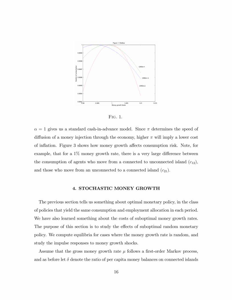
which has important effects on consumption risk. In Figure 1, we graph welfare

relative to optimal money growth, measured in units of consumption relative to what

is achieved with an optimal money growth rate, for different levels of the coefficient

of relative risk aversion. Note that the optimal money growth rate increases with the

coefficient of relative risk aversion, and that for a fairly moderate level of risk aversion

(CRRA = 2) a Þxed money supply is very close to optimal. That is, it does not take

a high degree of risk aversion for consumption risk to become the dominant force in

determining optimal monetary policy. Higher risk aversion of course also increases

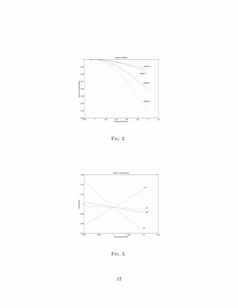
the welfare costs of deviations from the optimal money growth rate. In Figure 2 we

show the same picture as in Figure 1, but we include higher levels for the money

growth rate. With CRRA = .5, the welfare loss from a 10% per period inßation is

somewhat more than 1% of consumption, but this number increases to more than 7%

of consumption for CRRA = 3, a cost which is very large relative to what is typically

obtained in the literature. The welfare cost of inßation also depends critically on

α and π. The larger is α, the lower is the cost of inßation. Note in particular that

15

0.99 0.995 1 1.005 1.01 1.0150.9993

0.9994

0.9995

0.9996

0.9997

0.9998

0.9999

1Figure 1: Welfare

Money growth factor

fract

ion

of c

onsu

mpt

ion

CRRA=.5

CRRA=1

CRRA=2

Fig. 1.

α = 1 gives us a standard cash-in-advance model. Since π determines the speed of

diffusion of a money injection through the economy, higher π will imply a lower cost

of inßation. Figure 3 shows how money growth affects consumption risk. Note, for

example, that for a 1% money growth rate, there is a very large difference between

the consumption of agents who move from a connected to unconnected island (c12),

and those who move from an unconnected to a connected island (c21).

4. STOCHASTIC MONEY GROWTH

The previous section tells us something about optimal monetary policy, in the class

of policies that yield the same consumption and employment allocation in each period.

We have also learned something about the costs of suboptimal money growth rates.

The purpose of this section is to study the effects of suboptimal random monetary

policy. We compute equilibria for cases where the money growth rate is random, and

study the impulse responses to money growth shocks.

Assume that the gross money growth rate µ follows a Þrst-order Markov process,

and as before let δ denote the ratio of per capita money balances on connected islands

16

0.98 1 1.02 1.04 1.06 1.08 1.1 1.120.92

0.93

0.94

0.95

0.96

0.97

0.98

0.99

1Figure 2: Welfare

money growth factor

fract

ion

of c

onsu

mpt

ion

CRRA=.5

CRRA=1

CRRA=2

CRRA=3

Fig. 2.

0.99 0.995 1 1.005 1.01 1.0150.94

0.96

0.98

1

1.02

1.04

1.06Figure 3: Consumption

money growth factor

cons

umpt

ion

c11

c12

c21

c22

Fig. 3.

17

to per capita money balances on unconnected islands. Then, the state is described

by (µ, δ), and assuming that cash-in-advance constraints hold with equality, the law

of motion for δ is, using (10), (11), and (20),

δ0 =α[µ0 − (1− α)π]δ + (1− α)(µ0 − 1 + απ)

α2πδ + α(1− απ) , (33)

where primes denote variables dated t + 1. Therefore, if consumers spend all of the

household�s cash balances each period, then the stochastic process for δ is exogenous,

which makes computing equilibria relatively straightforward. It is clear from (33)

that there is persistence in δ, due to the fact that it takes time for a money shock to

diffuse. The diffusion rate is governed by π. Note that, if π = 0, then (33) gives

δ0 =µ0 − 1 + α

α,

in which case the distribution of money balances across the population is determined

only by the current money growth rate, and there is no persistence.

In this environment, the Þrst-order conditions from the optimization problems of

households on connected and unconnected islands, respectively, yield

−v0(n1t) + βZ ½

p1t[1− (1− α)π]u0(c11t+1)p1,t+1

+p1t(1− α)πu0(c12t+1)

p2,t+1

¾dF (µ0;µ) = 0,

(34)

−v0(n2t) + βZ ½

p2tαπu0(c21t+1)

p1,t+1+p2t(1− απ)u0(c22t+1)

p2,t+1

¾dF (µ0;µ) = 0, (35)

where F (µ0;µ) is the distribution of µ0 conditional on µ. Let ni(δ, µ) denote the level of

employment in state (δ, µ), where i = 1 denotes a connected island and i = 2 denotes

an unconnected island. Then, substituting in (34) and (35) using the equilibrium

conditions (12) and (13) and using (20), we get

18

−v0[n1(δ, µ)]n1(δ, µ)

+β

Z [1− (1− α)π]u0h

n1(δ0,µ0)δ0

[1−(1−α)π]δ0+(1−α)πi h

n1(δ0,µ0){[1−(1−α)π]δ+(1−α)π}

φ1(µ0,δ)

i+(1− α)πu0

hn2(δ

0,µ0)δ0απδ0+1−απ

i hn2(δ

0,µ0){[1−(1−α)π]δ+(1−α)π}φ2(µ

0,δ)

i dF (µ0;µ)

= 0, (36)

−v0[n2(δ, µ)]n2(δ, µ)

+β

Z απu0h

n1(δ0,µ0)

[1−(1−α)π]δ0+(1−α)πi h

n1(δ0,µ0)[απδ+1−απ]φ1(µ

0,δ)

i+(1− απ)u0

hn2(δ

0,µ0)δ0απδ0+1−απ

i hn2(δ

0,µ0)[απδ+1−απ]φ2(µ

0,δ)

i dF (µ0;µ) = 0, (37)

and the consumption allocations are

c11(δ, µ) =n1(δ, µ)δ

[1− (1− α)π] δ + (1− α)π , (38)

c12(δ, µ) =n2(δ, µ)δ

απδ + 1− απ, (39)

c22(δ, µ) =n2(δ, µ)δ

απδ + 1− απ, (40)

c21(δ, µ) =n1(δ, µ)

[1− (1− α)π] δ + (1− α)π . (41)

In (36) and (37) δ0 is determined by (33) and the functions φi(µ0, δ) for i = 1, 2, are

deÞned by

φ1(µ0, δ) ≡ {µ0 [1− (1− α)π]− (1− α)π(1− π)} δ

+(1− α)½(µ0 − 1) [1− (1− α)π]

α+ π(2− π)

¾,

φ2(µ0, δ) ≡ απ (µ+ 1− π) δ + (1− απ)(1− π) + µ0π(1− α).

19

Numerical Exercises

As with the constant money growth experiments, we use u(c) = c1−γ−11−γ , with γ > 0

and v(n) = n. We set β = .99, γ = 1.5, α = .2, and π = .1. Thus, we use parameter

values such that monetary shocks will initially affect few agents and the shocks will

have highly-persistent effects. As well, we will look only at examples where money

growth shocks are i.i.d., as in this case there would be no effect of a money shock

on employment, output, and consumption in the special case where there are no

distribution effects (α = 1). In this case, all of the persistence in the effects of money

shocks will come from persistent effects on the distribution of money balances across

the population.

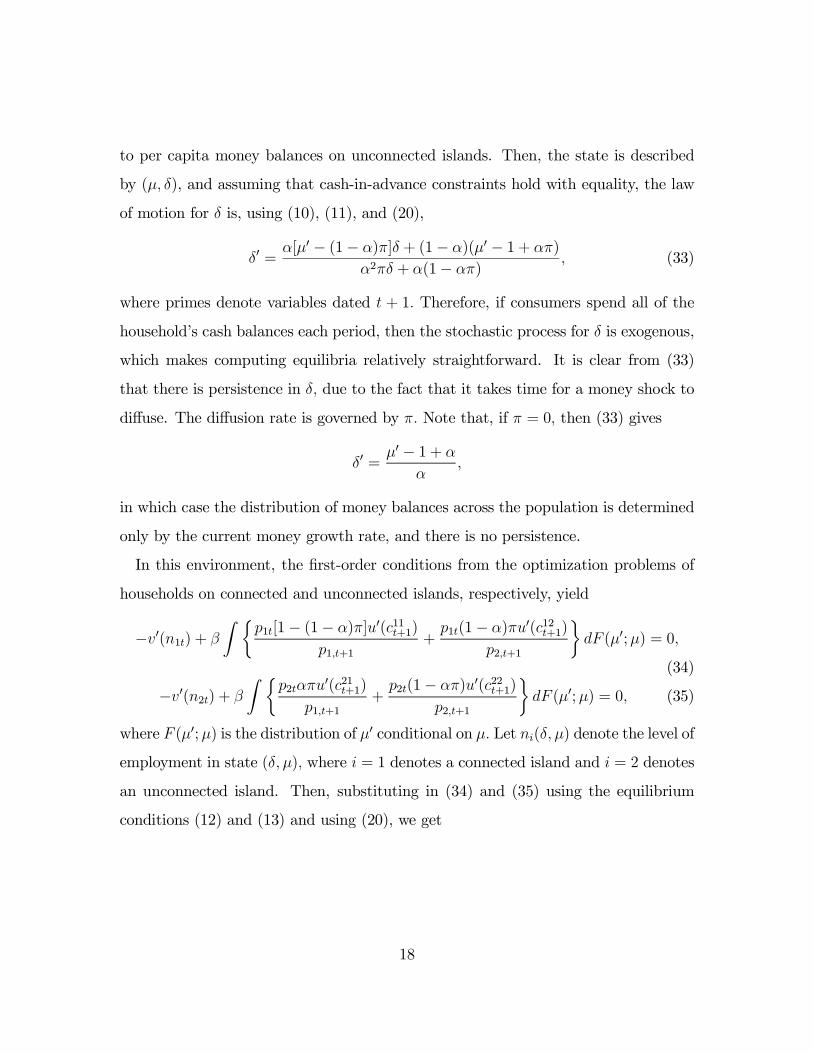
In the Þrst experiment, we look at an economy where the money growth factor

takes on values over a uniform grid on [1, 1.02], with equal probability mass on each

point in the grid. Therefore, the mean gross growth rate of the money stock is 1.01.

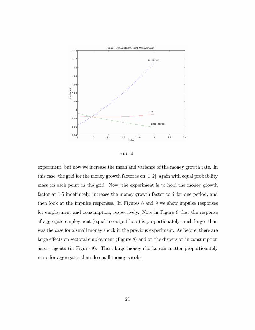
Since the money growth factor is i.i.d., the state variable is δ, and Figures 4 and

5 show the optimal decision rules for employment and consumption, respectively.

We then study an experiment where we suppose that the money growth factor has

been at 1.01 indeÞnitely, and then study the impulse responses to a shock where the

money growth factor increases for one period to 1.02 and then returns to 1.01 forever.

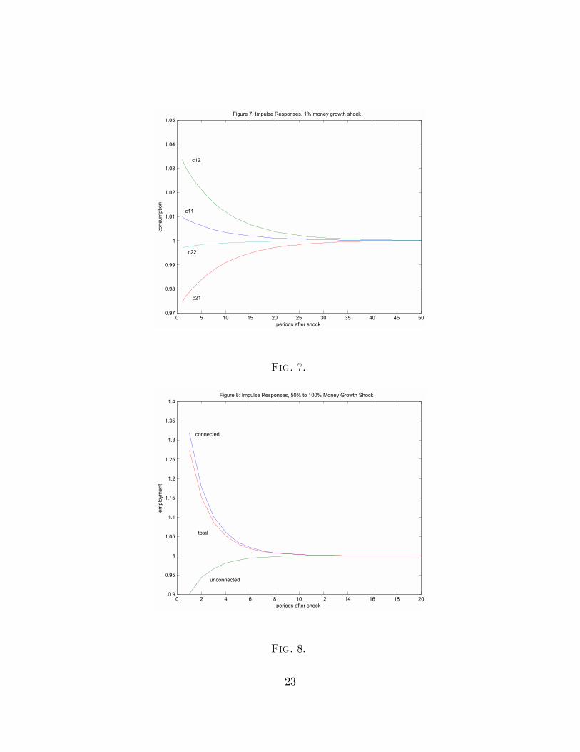
Figures 6 and 7 show the impulse responses of employment and consumption. Note

that the sectoral effects are large in that employment in connected locations increases

substantially and employment in unconnected locations falls substantially, and there

is a signiÞcant increase in the dispersion of consumption across agents. However,

there is only a very small increase in aggregate output and employment. Therefore,

small money shocks can be important for sectoral consumption and employment (and

presumably welfare), but have little effect on aggregates.

For the second experiment, parameters are identical to what we used for the Þrst

20

1 1.2 1.4 1.6 1.8 2 2.2 2.40.94

0.96

0.98

1

1.02

1.04

1.06

1.08

1.1

1.12

1.14Figure4: Decision Rules, Small Money Shocks

delta

empl

oym

ent

connected

unconnected

total

Fig. 4.

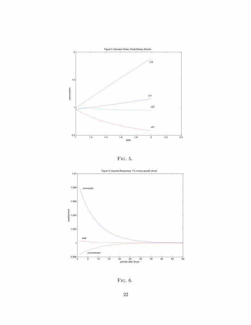
experiment, but now we increase the mean and variance of the money growth rate. In

this case, the grid for the money growth factor is on [1, 2], again with equal probability

mass on each point in the grid. Now, the experiment is to hold the money growth

factor at 1.5 indeÞnitely, increase the money growth factor to 2 for one period, and

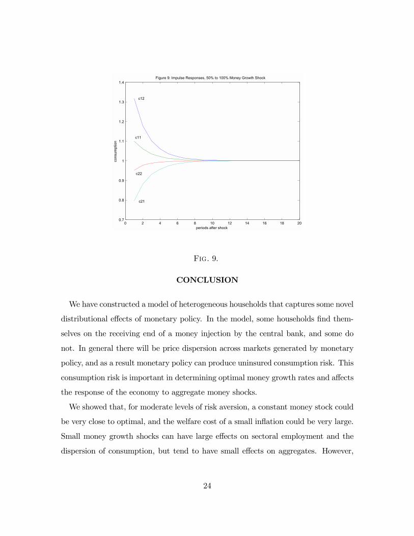
then look at the impulse responses. In Figures 8 and 9 we show impulse responses

for employment and consumption, respectively. Note in Figure 8 that the response

of aggregate employment (equal to output here) is proportionately much larger than

was the case for a small money shock in the previous experiment. As before, there are

large effects on sectoral employment (Figure 8) and on the dispersion in consumption

across agents (in Figure 9). Thus, large money shocks can matter proportionately

more for aggregates than do small money shocks.

21

1 1.2 1.4 1.6 1.8 2 2.2 2.40.5

1

1.5

2Figure 5: Decision Rules, Small Money Shocks

delta

cons

umpt

ion

c11

c22

c21

c12

Fig. 5.

0 5 10 15 20 25 30 35 40 45 500.998

1

1.002

1.004

1.006

1.008

1.01Figure 6: Impulse Responses, 1% money growth shock

periods after shock

empl

oym

ent

connected

unconnected

total

Fig. 6.

22

0 5 10 15 20 25 30 35 40 45 500.97

0.98

0.99

1

1.01

1.02

1.03

1.04

1.05Figure 7: Impulse Responses, 1% money growth shock

periods after shock

cons

umpt

ion

c11

c12

c21

c22

Fig. 7.

0 2 4 6 8 10 12 14 16 18 200.9

0.95

1

1.05

1.1

1.15

1.2

1.25

1.3

1.35

1.4Figure 8: Impulse Responses, 50% to 100% Money Growth Shock

periods after shock

empl

oym

ent

connected

unconnected

total

Fig. 8.

23

0 2 4 6 8 10 12 14 16 18 200.7

0.8

0.9

1

1.1

1.2

1.3

1.4Figure 9: Impulse Responses, 50% to 100% Money Growth Shock

periods after shock

cons

umpt

ion

c11

c12

c21

c22

Fig. 9.

CONCLUSION

We have constructed a model of heterogeneous households that captures some novel

distributional effects of monetary policy. In the model, some households Þnd them-

selves on the receiving end of a money injection by the central bank, and some do

not. In general there will be price dispersion across markets generated by monetary

policy, and as a result monetary policy can produce uninsured consumption risk. This

consumption risk is important in determining optimal money growth rates and affects

the response of the economy to aggregate money shocks.

We showed that, for moderate levels of risk aversion, a constant money stock could

be very close to optimal, and the welfare cost of a small inßation could be very large.

Small money growth shocks can have large effects on sectoral employment and the

dispersion of consumption, but tend to have small effects on aggregates. However,

24

large money growth shocks can have proportionately large effects on aggregate output,

employment, and consumption.

REFERENCES

Alvarez, F. and Atkeson, A. 1997. �Money and Exchange Rates in the Grossman-

Weiss-Rotemberg Model,� Journal of Monetary Economics 40, 619-40.

Alvarez, F., Atkeson, A., and Kehoe, P. 2002. �Money, Interest Rates, and Exchange

Rates with Endogenously Segmented Markets,� Journal of Political Economy

110, 73-112.

Chiu, J. 2005. �Endogenously Segmented Asset Market in an Inventory Theoretic

Model of Money Demand,� working paper, University of Western Ontario.

Grossman, S. and Weiss, L. 1983. �A Transactions-Based Model of the Monetary

Transmission Mechanism,� American Economic Review 73, 871-880.

Head, A. and Shi, S. 2003. �A Fundamental Theory of Exchange Rates and Direct

Currency Trades,� Journal of Monetary Economics 50, 1555-1592.

Lagos, R., and Wright, R. 2005. �A UniÞed Framework for Monetary Theory and

Policy Analysis,� forthcoming, Journal of Political Economy.

Lucas, R. 1990. �Liquidity and Interest Rates,� Journal of Economic Theory 50,

237-264.

Rotemberg, J. 1984. �A Monetary Equilibrium Model with Transactions Costs,�

Journal of Political Economy 92, 40-58.

Shi, S. 1997. �A Divisible Model of Fiat Money,� Econometrica 65, 75-102.

25

Shi, S. 2004. �Liquidity, Interest Rates, and Output,� working paper, University of

Toronto.

Williamson, S. 2005. �Search, Limited Participation, and Monetary Policy,� forth-

coming, International Economic Review.

26