Federal Reserve Bank of Minneapolis

Research Department

Monetary Policy and Dutch Disease:The Case of Price and Wage Rigidity∗

Constantino Hevia and Juan Pablo Nicolini

Working Paper 726

June 2015

ABSTRACT

We study a model of a small open economy that specializes in the production of commodities and

that exhibits exogenous frictions in the setting of both prices and wages. We study the optimal

response of monetary and exchange rate policy following a positive (negative) shock to the price

of the exportable that generates an appreciation (depreciation) of the local currency. According to

the calibrated version of the model, deviations from full price stability can generate welfare gains

that are equivalent to almost 05% of lifetime consumption, as long as there is a significant degree

of rigidity in nominal wages. On the other hand, if the rigidity is concentrated in prices, the welfare

gains can be at most 01% of lifetime consumption. We also show that a rule–formally defined in the

paper–that resembles a “dirty floating” regime can approximate the optimal policy remarkably well.

Keywords: Dutch disease; Inflation targeting; Foreign exchange intervention

JEL classification: F31, F41

∗Hevia: Universidad Di Tella. Nicolini: Federal Reserve Bank of Minneapolis and Universidad Di Tella. Thispaper was prepared for the 18th annual conference of the Central Bank of Chile. We thank Cesar Calderon

for the discussion and Rodrigo Caputo and Roberto Chang for very detailed comments on an earlier draft.

The views expressed herein are those of the authors and not necessarily those of the Federal Reserve Bank of

Minneapolis or the Federal Reserve System.

1. INTRODUCTION

In this paper, we study optimal monetary and exchange rate policy in a small open economy

with both price and wage rigidity, following a shock to the price of an exportable commodity.

From a theoretical point of view, and as we show in the paper, the presence of both types of

rigidities implies that, to the extent that �scal policy is unresponsive to shocks, full price stability

is not optimal.

This paper is part of a research project that is motivated by the experiences of many small

open economies that in the last two decades became� very e¤ectively!� in�ation targeters. Many

of these economies are commodity producers, and the size of the commodity sector to GDP is

very high. For example, in the decade from 2000 to 2010, exports of copper and marine products

for Chile were, on average, around 17% of GDP, while total exports of oil and marine products

in Norway accounted for 20% of GDP (Hevia and Nicolini, 2013). During the same decade, the

real price of copper and oil experienced changes of around 300%. The size of these shocks is

orders of magnitude above any business cycle shock we have ever seen.

These shocks have direct e¤ects on the monetary side of these economies. In e¤ect, the cor-

relation between the HP-�ltered price of the exportable commodity and the HP-�ltered nominal

exchange rate� to concentrate our analysis at the business cycle frequency� ranges from �50%

to �70% for both countries, depending on whether one includes the last three periods of the

decade in the sample. That period of time witnessed very large changes in commodity prices,

comoving with the peso in Chile and the krone in Norway.1 In Figure 1, we plot the HP-�ltered

data for the nominal exchange rate and the relevant commodity price for both countries, where

the correlation is strikingly clear.

Clearly, this correlation cannot be independent of the policy regime. In a currency board

or �xed exchange rate regime, that correlation is naturally zero. Thus, one should expect the

1The series are �rst logged and then HP-�ltered with a smoothing parameter of 1600.

1

2000 2002 2004 2006 2008 2010 2012­80

­60

­40

­20

0

20

40

60Chile

2000 2002 2004 2006 2008 2010 2012­80

­60

­40

­20

0

20

40

60Norway

Exchange ratePrice of copper

Exchange ratePrice of oil

Fig. 1. Nominal exchange rates and main exportable commodity price

correlation between the price of copper and the exchange rate in Chile to be much closer to zero

during the early nineties, during which time in�ation was driven down from close to 30% to

below 10% using a managed exchange rate. But in a very successful in�ation-targeting regime,

like the ones followed by both central banks during the period, the nominal exchange rate freely

�oats, so the correlation is determined by market forces. According to the model that follows, the

negative correlation is a direct implication of the in�ation-targeting regime. Indeed, in the model,

following a large increase in the price of the exportable, and given price stability, the nominal

exchange rate� and the real, given price stability� su¤ers a strong appreciation, generating the

traditional Dutch disease e¤ect, which is the optimal response of prices and quantities to a

relative price shock.

We are interested in studying conditions under which the strict in�ation-targeting regime is

optimal. Put di¤erently, we want to �nd conditions under which these Dutch disease episodes

are ine¢ cient from the viewpoint of the allocation of resources. In our view, this is one of the

main policy questions in countries like Chile. Indeed, during the successful in�ation-targeting

2

period, the central bank deviated from the strict rule twice: once in April 2008 and again in

January 2011. On both occasions, the justi�cation for the intervention was essentially the same:

the terms of trade were too high and the nominal exchange rate too low.

In a previous paper (Hevia and Nicolini, 2013), we studied an economy with only price frictions

and showed that even in a second best environment with distorting taxes, domestic price stability

is optimal as long as preferences are of the isoelastic type (which is typically used in the literature),

even if �scal policy cannot respond to shocks. In other words, restrictions on price setting do not

necessarily imply that the large and persistent deviations observed in nominal and real exchange

rates in countries like Chile are suboptimal, as long as monetary policy is executed so as to

stabilize domestic prices. The model in that paper thus fully justi�es a pure in�ation targeting

regime (at a zero rate of domestic price in�ation). In other words, the �Dutch disease� is not

really a disease, it is just the optimal response of prices and quantities to a relative price shock.

In the conclusion to our previous paper, we pointed out that our results fall apart in the

presence of both price and wage frictions. Quantitatively exploring this question is the purpose

of this paper. Exploring this policy problem in the context of both price and wage rigidity seems

to us a natural step. Most medium-scale models used for monetary policy evaluation nowadays

exhibit both types of rigidities, following the work of Christiano, Eichenbaum, and Evans (2005)

and Smets and Wouters (2007). How far from pure price stability is the optimal policy once both

types of frictions are present? What implications do they have for the �dirty �oating�debate in

countries that experience large �uctuations in their terms of trade? Answering these questions

is the contribution of this paper.

As mentioned, the theory is clear: the presence of both frictions, coupled with in�exible tax

instruments, implies that full price stability is not optimal. For completeness, we �rst generalize

the closed economy results of Correia et al. (2013) and the small open economy results of Hevia

and Nicolini (2013) with only price frictions to our small open economy model with price and

wage frictions and then show that, in general, full price stability is not optimal when taxes cannot

3

be time and state dependent. But the main exploration of this paper is a quantitative one: on

the one hand, we explore numerically how far apart from full in�ation targeting the optimal

policy is; on the other, we compute the welfare di¤erence between the optimal policy and full

in�ation targeting. For the calibrated version of our model, we �nd that the key factor is the

degree of wage rigidity. When wages are indeed highly rigid (the Calvo parameter is as high as

0:8) and there is enough price rigidity (a Calvo parameter of at least 0:25), the welfare e¤ect of

full price stability relative to the optimal policy can be as high as 0:5% of lifetime consumption.

However, if the rigidity is mostly concentrated in prices with some wage rigidity, the welfare

e¤ect is bounded above by 0:1% of lifetime consumption. We also show that a dirty �oating

regime approximates the optimal policy remarkably well.

The model we use is the one explored in Hevia and Nicolini (2013), but in this model, we allow

for heterogeneous labor with market power and frictions in wage setting. A virtue of the model

is that it is fully consistent with the evidence presented in Figure 1, as we show in the paper. We

present the model in Section 2. In Section 3 we describe the calibration and numerical solutions

and discuss optimal policy. A �nal section concludes.

2. THE MODEL

We study a discrete time model of a small open economy inhabited by households, the gov-

ernment, competitive �rms that produce a tradable commodity, competitive �rms that produce

�nal goods, and a continuum of �rms that produce di¤erentiated intermediate goods. There

are two di¤erentiated traded �nal goods: one produced at home and the other produced in

the rest of the world. The small open economy faces a downward-sloping demand for the �nal

good it produces but takes as given the international price of the foreign �nal good. There are

also two commodities� one produced at home, the other imported� used in the production of

intermediate goods. These intermediate goods are used to produce the �nal domestic good.

4

Households

A representative household has preferences over contingent sequences of two �nal consumption

goods, Cht and C

ft , and leisure Lt. The utility function is weakly separable between the �nal

consumption goods and leisure and is represented by

E0

1Xt=0

�tU (Ct; Lt) ; (1)

where 0 < � < 1 is a discount factor, Ct = H(Cht ; C

ft ) is a function homogeneous of degree one

and increasing in each argument, and U (C;L) is concave and increasing in both arguments.

Sticky Wages. In order to allow for sticky wages, we assume the single household has a

continuum of members indexed by h 2 [0; 1], each supplying a di¤erentiated labor input nht.

Preferences of the household are described by (1), where leisure is

Lt = �L�Z 1

0

nhtdh; (2)

and �L is the total amount of time available for work or for leisure.

The di¤erentiated labor varieties aggregate up to total labor input Nt, used in production,

according to the Dixit-Stiglitz aggregator

Nt =

�Z 1

0

nht�w�1�w dh

� �w

�w�1

; �w > 1: (3)

Each member of the household, which supplies a di¤erentiated labor variety, behaves under

monopolistic competition. The workers set wages as in Calvo (1983), with the probability of

being able to revise the wage 1 � �w. This lottery is i:i:d: across workers and over time. The

workers that are not able to set wages in period 0 all share the same wage w�1. Other prices

5

are taken as given. There is a complete set of state-contingent assets. We consider an additional

tax, a payroll tax on the wage bill paid by �rms, � pt .

Market Structure Financial markets are complete. We let Bt;t+1 and B�t;t+1 denote one-

period discount bonds denominated in domestic and foreign currency, respectively. These are

bonds issued at period t that pay one unit of the corresponding currency at period t + 1 on a

particular state of the world and zero otherwise.

The household�s budget constraint is given by

P ht C

ht + P f

t Cft + Et

hQt;t+1Bt;t+1 + StQ

�t;t+1

~B�t;t+1

i� (4)

Wt (1� �nt )Nt +Bt�1;t + St~B�t�1;t

1 + � �t;

where St is the nominal exchange rate between domestic and foreign currency, Wt is the nominal

wage rate, �nt is a labor income tax, ��t is a tax on the return of foreign-denominated bonds

(a tax on capital �ows), and Qt;t+1 is the domestic currency price of the one-period contingent

domestic bond normalized by the conditional probability of the state of the economy in period

t + 1 conditional on the state in period t. Likewise, Q�t;t+1 is the normalized foreign currency

price of the foreign bond.2 In this constraint, we assume that dividends are fully taxed and that

consumption taxes are zero (we explain these choices later).

Using the budget constraint at periods t and t + 1 and rearranging gives the no-arbitrage

condition between domestic and foreign bonds:

Qt;t+1 = Q�t;t+1�1 + � �t+1

� StSt+1

: (5)

Working with the present value budget constraint is convenient. To that end, for any k > 0, we

2We use the notation ~B�t;t+1 instead of simply B�t;t+1 to distinguish foreign bonds held by the household sector

from foreign bonds held by the aggregate economy.

6

letQt;t+k = Qt;t+1Qt+1;t+2:::Qt+k�1;t+k be the price of one unit of domestic currency at a particular

history of shocks in period t+k in terms of domestic currency in period t; an analogous de�nition

holds forQ�t;t+k. Iterating forward on (4) and imposing the no-Ponzi condition limt!1E0[Q0;tBt+

StQ�0;t~B�t ] � 0 gives

E0

1Xt=0

Q0;t

�P ht C

ht + P f

t Cft �Wt (1� �nt )Nt

�� 0; (6)

where we have assumed that initial �nancial wealth is zero, or B�1;0 = ~B��1;0 = 0.

The household maximizes (1) subject to (6). The optimality conditions are given by

HCh(Cht ; C

ft )

HCf (Cht ; C

ft )=P ht

P ft

(7)

UC (Ct; Lt)HCh(Cht ; C

ft )

P ht

= �1

Qt;t+1

UC (Ct+1; Lt+1)HCh(Cht ; C

ft )

P ht+1

; (8)

plus an optimal wage decision that will be discussed later.

Government

The government sets monetary and �scal policy and raises taxes to pay for exogenous con-

sumption of the home �nal good, Ght .3 Monetary policy consists of rules for either the nominal

interest rate Rt or the nominal exchange rate St. Fiscal policy consists of labor taxes �nt ; payroll

taxes �nt ; export and import taxes on foreign goods, �ht and �

ft , respectively; taxes on returns of

foreign assets � �t ; and dividend taxes �dt .

The two sources of pure rents in the model are the dividends of intermediate good �rms and

the pro�ts of commodity producers �equivalently, one can think of the latter as a tax on the

rents associated with a �xed factor of production. Throughout the paper, we assume that all

3It is straightforward to also let the government consume foreign goods.

7

rents are fully taxed so that � dt = 1 for all t. The reason for this assumption is that if pure rents

are not fully taxed, the Ramsey government will use other instruments to partially tax those

rents. We deliberately abstract from those e¤ects in the optimal policy problem.

Our description of �scal policy is for completeness. As is well known,4 when �scal policy

can respond to shocks and there is a complete set of instruments, price stability is optimal. The

taxes described in this section do represent a complete set of instruments. The optimal monetary

policy becomes nontrivial once �scal instruments are exogenously restricted to be unresponsive

to shocks.

Final good �rms

Perfectly competitive �rms produce the domestic �nal good Y ht by combining a continuum of

nontradable intermediate goods indexed by i 2 (0; 1) using the technology

Y ht =

�Z 1

0

y��1�

it di

� ���1

;

where � > 1 is the elasticity of substitution between each pair of intermediate goods. Taking as

given the �nal good price, P ht , and the prices of each individual variety of intermediate goods,

P hit for i 2 (0; 1), the �rm�s problem implies the cost minimization condition

yit = Y ht

�P hit

P ht

���(9)

for all i 2 (0; 1). Integrating this condition over all varieties and using the production function

gives a price index relating the �nal good price and the prices of the individual varieties,

P ht =

�Z 1

0

P h1��it di

� 11��

: (10)

4See Adao, Correia, and Teles (2009), Correia, Nicolini, and Teles (2008), Correia, Farhi, Nicolini, and Teles(2013), Farhi, Gopinath, and Itskhoki (2014), and Hevia and Nicolini (2013).

8

Minimization of labor costs

Before describing the technologies of the sectors that demand labor, we believe it is useful to

describe the labor cost minimization problem. Firms minimizeR 10whtnhtdh, where wht is the

wage of the h-labor, for a given aggregate Nt, subject to (3). The demand for nht is

nht =

�whtWt

���wNt, (11)

where Wt is the aggregate wage level, given by

Wt =

�Z 1

0

wht1��wdh

� 11��w

. (12)

It follows thatR 10whtnhtdh = WtNt.

The optimal wage-setting conditions by the monopolistic competitive workers are now

wt =�w

�w � 1Et1Xj=0

�wt;jUL (t+ j)

UC (t+ j)

(1 + � ct+j)Pt+j

(1� �nt+j); (13)

with

�wt;j =(1� �nt+j) (�

w�)j UC(t+j)

(1+�ct+j)Pt+j(Wt+j)

�w Nt+j

EtP1

j=0(1� �nt+j) (�w�)j UC(t+j)

(1+�ct+j)Pt+j(Wt+j)

�w Nt+j

: (14)

The wage level (12) can be written as

Wt =�(1� �w)w1��

w

t + �wW 1��wt�1

� 11��w . (15)

Using (11), we can write (2) as

Nt =

"Z 1

0

�whtWt

���wdh

#�1 ��L� Lt

�. (16)

9

From (12), it must be thatR 10

�whtWt

���wdh � 1. This means that for a given total time dedicated

to work, �L � Lt, the resources available for production are maximized when there is no wage

dispersion.

In equilibrium

�L� Lt = Nt

t+1Xj=0

$wj

�wt�jWt

���w;

where $wj is the share of household members that have set wages j periods before, $w

j =

(�w)j(1� �w), j = 0; 2; :::; t , and $wt+1 = (�

w)t+1, which is the share of workers that have never

set wages and charge the exogenous wage w�1.

Primary commodity sector

Two tradable commodities, denoted by x and z, are used as inputs in the production of

intermediate goods. The home economy, however, is able to produce only the commodity x;

the commodity z must be imported. We denote by P xt and P

zt the local currency prices of the

commodities.

Total output of commodity x; denoted as Xt; is produced according to the technology

Xt = At (nxt )� ; (17)

where nxt is labor, At is the level of productivity, and 0 < � � 1. Implicit in this technology is

the assumption of a �xed factor of production (when � < 1), which we broadly interpret as land.

Pro�t maximization implies

�P xt At (n

xt )��1 = Wt(1 + �

pt ): (18)

10

Because the two commodities can be freely traded, the law of one price holds:

P xt = StP

x�t (19)

P zt = StP

z�t ;

where P x�t and P z�

t denote the foreign currency prices of the x and z commodities.5

We can use (19) and (18) to obtain

�StPx�t At (n

xt )��1 = Wt(1 + �

pt );

which, given values for the exogenous shocks and given an allocation, restricts the feasible values

for fSt;Wt; �ptg:

Intermediate good �rms

Each intermediate good i 2 (0; 1) is produced by a monopolistic competitive �rm that uses

labor and the two tradable commodities with the technology

yit = ��Ztx�1it z

�2it (n

yit)�3 ;

where xit and zit are the demand for commodities, nyit is labor, Zt denotes the level of productivity,

�j � 0 for j = 1; 2; 3,P3

j=1 �j = 1, and �� = ���11 �

��22 �

��33 .

The associated nominal marginal cost function is common across intermediate good �rms and

given by

MCt =(P x

t )�1 (P z

t )�2W

�3t (1 + �

pt )�

�3

Zt:

Using (18) and (19), the nominal marginal cost can be written as MCt = StMC�t , where MC�t ,

5We could also allow for tari¤s on the intermediate inputs. However, these tari¤s are redundant instrumentsin this environment.

11

the marginal cost measured in foreign currency, is given by

MC�t =(P x�

t )1��2 (P z�

t )�2 (�At (n

xt )��1 (1 + � pt ))

�3

Zt: (20)

That is, the marginal cost in foreign currency depends on the international commodity prices,

on technological factors, and on the equilibrium allocation of labor in the commodities sector.

In addition, cost minimization implies that �nal intermediate good �rms choose the same ratio

of inputs,

xitnyit

=�1�3�At (n

xt )��1 (1 + � pt ) (21)

zitnyit

=�2�3

P x�t

P z�t

�At (nxt )��1 (1 + � pt ) for all i 2 (0; 1) ;

where we have used (18) in the second equation.

Introducing (21) into the production function gives

yit = nyitZt�3(�At (n

xt )��1 (1 + � pt ))

1��3 (P x�t )

�2 (P z�t )

��2 : (22)

Each monopolist i 2 (0; 1) faces the downward-sloping demand curve (9). We follow the

standard tradition in the New Keynesian literature and impose Calvo price rigidity. Namely,

in each period, intermediate good �rms are able to reoptimize nominal prices with a constant

probability 0 < �p < 1. Those that get the chance to set a new price will set it according to

pht =�

� � 1Et1Xj=0

�t;j(P x

t+j)�1(P z

t+j)�2�Wt+j(1 + �

pt+j)��3

Zt+j; (23)

where

�t;j =�pjQt;t+j(P

ht+j)

�Y ht+j

EtP1

j=0 �jQt;t+j(P h

t+j)�Y h

t+j

: (24)

12

The price level in (10) can be written as

P ht =

h(1� �p)

�pht�1��

+ �p�P ht�1�1��i 1

1��. (25)

Foreign sector and feasibility

We assume an isoelastic foreign demand for the home �nal good of the form

Ch�t = (K�

t )� �P h�

t

���; (26)

where > 1, P h�t is the foreign currency price of the home �nal good, and K�

t is a stochastic

process that transforms units of foreign currency into domestic consumption goods.6

The government imposes a tax (1 + �ht ) on �nal goods exported to the rest of the world and

a tari¤ (1 + � ft ) to �nal good imports. The law of one price on domestic and foreign �nal goods

then requires

P ht (1 + �

ht ) = StP

h�t (27)

P ft = StP

f�t (1 + �

ft );

where P f�t is the foreign currency price of the foreign �nal good.

Net exports measured in foreign currency are given by

m�t = P h�

t Ch�t � P f�

t Cft + P x�

t

�Xt �

Z 1

0

xitdi

�� P z�

t

Z 1

0

zitdi: (28)

6We allow for the �nal goods to be traded, so a particular case of our model (the one with A = 0 and�1 = �2 = 0) without commodities is the one typically analyzed in the small open economy New Keynesianliterature.

13

Thus, the net foreign assets of the country, denoted by B�t;t+1, evolve according to

B�t�1;t +m�

t = EtB�t;t+1Q

�t;t+1: (29)

Solving this equation from period 0 forward, and assuming zero initial foreign assets, gives the

economy foreign sector feasibility constraint measured in foreign currency at time 0:

E0

1Xt=0

Q�0;tm�t = 0: (30)

In addition, market clearing in domestic �nal goods requires

Y ht = Ch

t + Ch�t +Gh

t ; (31)

and labor market feasibility is given by

Nt =

Z 1

0

nyitdi+ nxt : (32)

Fiscal and monetary policies

We now show how a �exible exchange rate system, coupled with a �exible payroll tax, can

jointly stabilize domestic prices and wages. First, using the law of one price for the commodities,

P xt = StP

x�t

P zt = StP

z�t ;

14

we can write the cost minimization condition in the commodity sector (18) and the marginal

cost for the intermediate good �rm as

�StPx�t At (n

xt )��1 = Wt(1 + �

pt )

MCt = St(P x�

t )1��2 (P z�

t )�2 (�At (n

xt )��1)�3

Zt:

Because domestic prices are proportional to marginal costs, they will be constant once marginal

costs are constant, which implies

MC = St(P x�

t )1��2 (P z�

t )�2 (�At (n

xt )��1)�3

Zt;

so the nominal exchange rate moves to absorb productivity and commodity price shocks. Note

that the negative correlation between the nominal exchange rate and the prices of the exportable

commodity, presented in Figure 1, follows as a direct result of price stability. We can then use

this implied equilibrium relationship to solve for the nominal exchange rate and use it on the

cost minimization condition of the commodity sector to obtain

�1��3MC

�P x�t

P z�t

��2ZtAt (n

xt )(��1)(1��3) = Wt(1 + �

pt ):

So, to stabilize wages, the payroll tax must move according to

(1 + � pt ) =1

W�1��3MC

�P x�t

P z�t

��2ZtAt (n

xt )(��1)(1��3) :

Clearly, to the extent that �scal policy cannot be jointly used with monetary policy, there is

a trade-o¤ between eliminating the distortion in prices and eliminating the distortion in wages.

The numerical analysis of that question is addressed in the next section.

15

3. CALIBRATION AND NUMERICAL ANALYSIS OF MONETARY POLICY

Before we start, clarifying one issue is important. So far, we have been silent with respect to

the implementation of particular equilibria through policy. Since the work of Sargent andWallace

(1975), a vast literature has developed that analyzed the problem of unique implementation using

particular policy targets. To brie�y summarize that literature, in general, when central banks use

money or the interest rate as the policy instrument, typically multiple equilibria are consistent

with a single policy rule. On the contrary, if the exchange rate is pegged, uniqueness typically

arises. Multiple solutions have been o¤ered. The most popular, in the context of interest rate

rules, is to only consider a bounded equilibrium and to assume rules that satisfy the Taylor

principle. We fully abstain from the issue of implementation and simply assume that policy

can successfully target a nominal variable (or a combination of two of them), such as prices of

domestic goods, P ht ; the nominal wage, Wt; or the nominal exchange rate, St.

We consider the following utility function:

U (C;L) =C1�

1� � &

��L� L

�1+ 1 +

;

where , &, and are positive parameters. The subutility function between domestic and foreign

�nal goods is of the constant elasticity of substitution form,

C = H�Ch; Cf

�=

�(1�$)1=�

�Ch���1

� +$1=��Cf���1

�

�;

where � is the elasticity of substitution between home and foreign goods, and $ is the share

parameter associated with the foreign good. As is common in the literature, $ can be interpreted

as the degree of openness of the economy.

Each time period in the model represents one quarter. Most of the parameters that we use

for calibrating the model are standard and reported in Table 1 in the appendix. We choose

16

� so that the discount factor is 0:95 on an annualized basis and set a standard risk aversion

parameter of = 2. The parameter is the reciprocal of the Frisch elasticity of labor supply.

We set = 1, which lies between the micro and macro estimates of this elasticity (Chetty et

al., 2011). Furthermore, this number is standard in the literature (see, for example, Catao and

Chang, 2013). The parameters & and �L de�ne units of measurement and are not important for

the quantitative results of the paper; we set & = 1 and choose �L so that in the steady state,

workers allocate one-third of their total available time to market activities.

The parameter � measures the Armington elasticity of substitution between home and foreign

�nal goods. Estimates of the Armington elasticity using microeconomic data tend to be much

higher than those based on macroeconomic data. We set � = 1:5; which is a common number

used in the international business cycles literature (Backus, Kehoe, and Kydland, 1994). This

value is also consistent with the macro estimates of the Armington elasticity reported in Feenstra

et al. (2014). We set the share parameter at $ = 0:2. This value is consistent with the observed

home bias in consumption (Obstfeld and Rogo¤, 2001) and is similar to that used in Catao and

Chang (2013).7

The production function of the home intermediates is characterized by the three share para-

meters, �1; �2, �3; and by the level of productivity Zt. We set the share parameters at �1 = 0:1,

�2 = 0:4, and �3 = 0:5: A labor share of about 50% is a standard parameterization. We set

�1 = 0:1 to capture the observation that the home commodity is not used intensively in the

production of home goods. The share of imported intermediate inputs �2 = 0:4 is not intended

to capture the import of a single commodity, such as oil in the case of Chile, but of a large

array of intermediate inputs and commodities used in the production of goods in the small open

economy. We normalize the long-run level of productivity to �Z = 1.

Regarding the technology to produce the home commodity, we set a small labor share of

7Galí and Monacelli (2005) and de Paoli (2009) use $ = 0:4: Quantitative results are similar if we set $ to0:4 instead of 0:2.

17

� = 0:1, to capture that the production of commodities is either land or capital intensive, and

set the steady-state level of technology, �A, at 0:2. With this calibration, the steady-state share of

labor in the commodities sector is about 0.15. This is the target number used in Hevia, Neumeyer,

and Nicolini (2013) using a broad de�nition of the commodity sector and an input-output matrix

for Chile (see the discussion in that paper for more details).

For the parameterization of the foreign demand of the home �nal good in equation (26), we

assume an elasticity of � = 1:5 and set K� to a constant value of 0:1. The foreign demand does

not play an important role in the simulations that we discuss later and, thus, these parameters

are almost irrelevant.

The parameters �p and �w determine the average number of periods between price and wage

adjustments. We follow Christiano, Eichenbaum, and Rebelo (2011) and set �w = 0:85. The

parameter �p is set at 0:5, which implies an expected price duration of two quarters. This is

consistent with the evidence in Klenow and Malin (2010).8 Finally, as is common in the literature,

we consider an e¢ cient steady state. This amounts to imposing a constant labor subsidy that

eliminates the monopolistic distortions, and a constant tari¤ that extracts the monopolistic

rents in the trade of the home �nal good. This follows because the small open economy faces a

downward-sloping foreign demand for the �nal good.

We now consider the calibration of the stochastic processes for the di¤erent shocks. We assume

that both productivity parameters, At and Zt, follow autoregressive processes of the form

log�At= �A

�= �A log

�At�1= �A

�+ "At

log�Zt= �Z

�= �Z log

�Zt�1= �Z

�+ "Zt;

where "At and "Zt are independent mean zero shocks with a standard deviation of �A and �Z ,

8The value used in Christiano, Eichenbaum, and Rebelo (2011) is �P = 0:85: As we show, the results changevery little if we use that value.

18

respectively. We values of these parameters are set at �A = �Z = 0:95 and �A = �Z = 0:013:

These are the standard values used in the literature of business cycles in small open economies

(Neumeyer and Perri, 2005).

It remains to calibrate the price processes. Commodity prices tend to be correlated among

them. One possibility is to calibrate the price processes by running a vector autoregression

(VAR) with the exportable and importable commodity prices. The problem with this approach,

however, is that it is not obvious how to identify the importable commodity. Indeed, while

exportable commodities are easily identi�ed, importable commodities are not concentrated in a

few goods. We thus proceed as follows. We calibrate the price process of the home commodity

by running a �rst-order autoregression using HP-�ltered world prices of copper de�ated by the

U.S. consumer price index over the period 2000�2014:

log�P x�t = �P x�� = �x log

�P x�t�1=

�P x��+ "xt;

where "xt � N (0; �2x) : The estimation delivers �x = 0:72 and �x = 0:016. We next impose a

VAR structure of the form264 log �P x�t = �P x��

log�P z�t =

�P z��375 =

264 �x �

� �z

375264 log

�P x�t = �P x��

log�P z�t�1= �P

z��375+

264 "xt

"zt

375 ;where �z = �x, so that the importable commodity is as persistent as the home commodity, but

�z = �x=2, re�ecting that shocks to a bundle of commodities will be less volatile than shocks to a

single commodity. Finally, we set the free parameter � so that the model is able to replicate the

correlation between the home commodity price and the nominal exchange observed in Chile over

the sample period discussed earlier. Setting � = 0:18 implies a correlation between the nominal

exchange rate and the commodity price of �0:63 under a policy of price stability. As a reference,

if we set � = 0; the latter correlation drops to �0:20.

19

In what follows, and given the policy rule we now discuss, we simulate the model by shutting

down all shocks except the commodity price P x�t : To approximate the solution of the model, we

use the quadratic perturbation method around the steady state developed by Schmitt-Grohé and

Uribe (2004).

The policy rule

In order to capture our interpretation of the recent Chilean experience, one could consider a

regime in which price stability is the main stated objective, but with some interventions to reduce

the volatility of the nominal exchange rate (similar to the interventions in 2008 and 2011).

Note that from the solution for the marginal cost, we can write

MCt = StMC�t ;

where

MC�t =(P x�

t )1��2 (P z�

t )�2 (�At (n

xt )��1)�3

Zt:

Clearly, MC�t �the marginal cost in foreign currency �is a function of the underlying shocks.

As we mentioned earlier, full price stability implies constant marginal costs in local currency, so

St =MC

MC�t:

We then allow for a general rule in which the deviations of the log of the nominal exchange

rate adjust a fraction of the deviations in the log of the marginal costs in foreign currency, or

d lnSt = ��d lnMC�t : (33)

Thus, when � = 1; we have pure in�ation targeting, when � = 0 we have a currency peg, and

20

by letting � 2 (0; 1) we can have all intermediate cases: the lower the value for �, the lower the

volatility of the nominal exchange rate and the larger the volatility of domestic in�ation. With

the policy rule so speci�ed, the model can be solved numerically.

The policy trade-o¤ implied by the previous rule may re�ect the one implied by dirty �oating

regimes, in which some intervention in foreign exchange markets is allowed. According to the

theory, dampening the movements in the nominal exchange rate implies increasing the volatility

of marginal costs and therefore the volatility of the price level. However, what seems a more

natural trade-o¤, given the nature of the two distortions, is stabilizing prices versus stabilizing

nominal wages. In the theory section, we showed how a payroll tax can be used together with

the nominal exchange rate to stabilize both prices and wages. Once the payroll tax cannot be

used, the nominal exchange rate can be used to stabilize either of them but not both. Thus, let

wht �Wt

P ht

:

Then, we can de�ne a policy where

d lnWt = �d lnwht : (34)

Thus, if � = 0; nominal wages are fully stabilized, whereas � = 1 implies full price stability.

The optimal policy is given by the value of � that maximizes welfare, given the process for the

exogenous shock� the price of the exportable commodity in this case. The earlier discussion

suggests that the optimal policy will indeed have � 2 (0; 1): This conjecture will be veri�ed

numerically later. In the appendix we discuss how we perform the welfare comparisons across

the di¤erent rules.

In view of the preceding discussion, we �rst consider the case in which the policy trades o¤

price stability with nominal wage stability, which is the trade-o¤ that will deliver the optimal

21

policy. Then, we discuss how the rule that trades o¤ price stability with nominal exchange rate

stability behaves, particularly compared with the optimal policy. We believe exploring this a

priori suboptimal rule is interesting for two reasons. First, it is the one that best approximates,

in our view, the dirty �oating policy debate, as our discussion of the recent Chilean experience

suggests. Second, while stabilizing wages in this simple model is trivial, it is much less so in a

real economy with so many sectors and so many di¤erent types of labor. It does seem to us that

focusing the policy debate on a single, extremely visible price is much more attractive.

The price/wage trade-o¤

We will �rst discuss the results using the general policy rule (34). To begin, we present

simulations for the model with the baseline calibration, except that we set the rigidity in wages

to be zero. The advantage of this case is that when prices are fully stabilized (� = 1), we obtain

the optimal allocation, which we use as a benchmark. In Figure 2 we show the impulse responses

for output, the real wage, the real exchange rate, and labor following a one-standard-deviation

positive shock to the price of the exportable, for several values of �. Throughout the paper,

output (GDP) is computed as the sum of the value added evaluated at the steady-state prices.

As expected, at the e¢ cient allocation (� = 1), there is a redistribution of labor toward the

exportable sector (labor increases by 14% in the commodity sector and drops by 0:8% in the

home good sector). Consumption of the home good becomes very expensive, so it goes down,

increasing total labor supply. This lowers the real wage and �rms hire more labor overall, so

GDP goes up by almost 0:35%. Since prices are stable, as the nominal exchange rate goes down,

so does the real exchange rate. When nominal wages are stabilized (� = 0), the same equilibria

would obtain by increases in the price level, if prices were fully �exible. But they are not, so the

drop in the real wage is lower in this case. Because the price of �nal goods does not go up as

much, demand for the �nal consumption good is relatively higher, so the drop in labor at the

22

0 5 10 15 200

0.05

0.1

0.15

0.2

0.25

0.3

0.35

Perc

. dev

. from

 stea

dy st

ate

ν = 0ν = 0.25ν = 0.5ν = 0.75ν = 1

0 5 10 15 20­1.4

­1.2

­1

­0.8

­0.6

­0.4

­0.2

0

0 5 10 15 20­2.5

­2

­1.5

­1

­0.5

0

0 5 10 15 200

0.2

0.4

0.6

0.8

1

1.2

1.4

1.6

1.8

Perc

. dev

. from

 stea

dy st

ate

Horizon0 5 10 15 20

0

5

10

15

Horizon0 5 10 15 20

­1

­0.8

­0.6

­0.4

­0.2

0

0.2

0.4

Horizon

Fig. 2. Economy with no wage rigidities

home good sector is smaller and the increase in GDP is higher (although the e¤ect is small).

Because the price level does not increase enough, the real exchange rate does not drop very much.

An interesting feature that arises from Figure 2 is that the e¤ect of the policy regime (from

a �xed exchange rate to a fully �oating one in which prices are stabilized) does not have a very

big impact on the transmission mechanism of a commodity price shock, even with a relatively

high value for the Calvo parameter (�p = 0:5). The larger di¤erences are in the movements of

the real wage and the real exchange rate, but not on the real allocation, which is what matters

for welfare.

The e¤ect of the policy regime is much more dramatic for the benchmark calibration (with

�w = 0:85), in which the optimal allocation cannot be implemented because of the presence

of both price and wage rigidity. We show the relevant impulse responses in Figure 3. When

policy fully stabilizes nominal wages, the behavior of labor and output is relatively similar to

23

the e¢ cient allocation: total output goes up by about 0:35%; total labor goes up by about 1:7%;

and the labor reallocation is very similar. Note, however, that fully stabilizing nominal prices

delivers a very di¤erent outcome: GDP falls by 0:3% and total labor by 0:2%.

0 5 10 15 20­0.4

­0.3

­0.2

­0.1

0

0.1

0.2

0.3

0.4

Per

c. d

ev. 

from

 ste

ady 

stat

e ν = 0ν = 0.25ν = 0.5ν = 0.75ν = 1

0 5 10 15 20­1.4

­1.2

­1

­0.8

­0.6

­0.4

­0.2

0

0 5 10 15 20­3.5

­3

­2.5

­2

­1.5

­1

­0.5

0

0 5 10 15 20­0.2

0

0.2

0.4

0.6

0.8

1

1.2

1.4

1.6

1.8

Per

c. d

ev. 

from

 ste

ady 

stat

e

Horizon0 5 10 15 20

0

2

4

6

8

10

12

14

Horizon0 5 10 15 20

­1.6

­1.4

­1.2

­1

­0.8

­0.6

­0.4

­0.2

0

0.2

Horizon

Fig. 3. Baseline economy

We also solved the model by setting the share of foreign goods to 0:01 and 0:4 (the benchmark

is 0:2) and the degree of price stickiness to 0:25 and 0:85 (the benchmark is 0:5). The results,

presented in the appendix, are roughly similar.

Finally, we switched the degree of rigidity between prices and wages, relative to the benchmark.

That is, we increased the degree of price rigidity to �p = 0:85 and reduced the degree of wage

rigidity to �w = 0:5: Results are depicted in Figure 4. Now, the choice of the policy regime

is much less relevant than in the benchmark case. As can be seen, full price stability delivers

outcomes that are very similar to the optimal allocation: an increase in output a bit below 0:35%,

an increase in total labor close to 1:6%, and a very similar labor reallocation. This is natural,

24

0 5 10 15 20­0.05

0

0.05

0.1

0.15

0.2

0.25

0.3

0.35

0.4

Perc

. dev

. from

 stea

dy st

ate

ν = 0ν = 0.25ν = 0.5ν = 0.75ν = 1

0 5 10 15 20­1.4

­1.2

­1

­0.8

­0.6

­0.4

­0.2

0

0.2

0 5 10 15 20­2.5

­2

­1.5

­1

­0.5

0

0 5 10 15 200

0.2

0.4

0.6

0.8

1

1.2

1.4

1.6

1.8

Perc

. dev

. from

 stea

dy st

ate

Horizon0 5 10 15 20

0

2

4

6

8

10

12

14

Horizon0 5 10 15 20

­1

­0.8

­0.6

­0.4

­0.2

0

0.2

0.4

Horizon

Fig. 4. Economy with higher price and lower wage rigidity

given that it is in the setting of prices where we have the largest friction. However, notice that

the e¤ects of a regime that fully stabilizes nominal wages do not a¤ect the allocation very much:

it generates an ine¢ ciently larger expansion, but it is small nonetheless (0:4% instead of 0:35%).

For a better visual comparison, in Figure 5 we plot the impulse responses of output, the real

wage, and labor in the �nal good sector for the benchmark case (�p = 0:5 and �w = 0:85) and

for this last case analyzed, in which the degrees of rigidity between prices and wages have been

switched (�p = 0:85 and �w = 0:5) using the same scales. The di¤erence is remarkable.

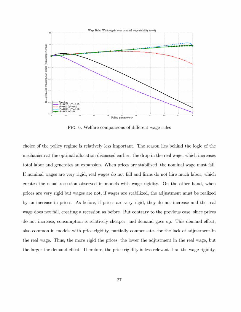
The welfare analysis is in line with the previous discussion. We show in Figure 6 the welfare

gain, in units of lifetime consumption, of alternative values of � 2 [0; 1], relative to the regime

� = 0; which is equivalent to full wage stability. Naturally, for the case in which �w = 0; full price

stability is optimal, which is re�ected in the fact that the line with circles is always increasing.

Note, however, that the opposite policy, the one that fully stabilizes wages (� = 0), entails a cost

25

0 5 10 15 20­0.4

­0.3

­0.2

­0.1

0

0.1

0.2

0.3

0.4

Perc

. dev

. from

 ste

ady 

stat

eν = 0ν = 0.25ν = 0.5ν = 0.75ν = 1

0 5 10 15 20

­1.2

­1

­0.8

­0.6

­0.4

­0.2

0

0 5 10 15 20­1.5

­1

­0.5

0

0.5

0 5 10 15 20­0.4

­0.3

­0.2

­0.1

0

0.1

0.2

0.3

0.4

Perc

. dev

. from

 ste

ady 

stat

e

Horizon0 5 10 15 20

­1.2

­1

­0.8

­0.6

­0.4

­0.2

0

Horizon0 5 10 15 20

­1.5

­1

­0.5

0

0.5

Horizon

Fig. 5. Comparison of di¤erent degrees of price and wage rigidities under the wage rule

of only 0:1% of lifetime consumption. On the other hand, for our baseline parameterization, the

optimal policy is slightly below � = 0:1; which amounts to almost full nominal wage stability.

Notice that in this case, which exhibits a high degree of wage rigidity, the welfare cost of full

price stability is over 0:45% of lifetime consumption, almost �ve times more. This is in line

with our previous discussion: when there is a high degree of wage rigidity and some degree of

price rigidity, the choice of the policy regime becomes more relevant. Notice that lowering the

degree of price rigidity to �p = 0:25 makes the optimal policy be even closer to full nominal wage

stability. Still, the e¤ect of the policy regime (the value for �) is very relevant. Finally, when

the wage rigidity is lowered to �w = 0:5; the optimal regime becomes close to � = 0:5, and the

e¤ect of full price stability becomes lower than 0:1% of lifetime consumption.

Overall, our results imply that the policy regime is much more relevant when there is a sub-

stantial degree of wage rigidity, coupled with some rigidity in the setting of prices. On the other

hand, if there is a high degree of price stickiness, coupled with some degree of wage rigidity, the

26

0 0.1 0.2 0.3 0.4 0.5 0.6 0.7 0.8 0.9 1­0.5

­0.4

­0.3

­0.2

­0.1

0

0.1

0.2

Fig. 6. Welfare comparisons of di¤erent wage rules

choice of the policy regime is relatively less important. The reason lies behind the logic of the

mechanism at the optimal allocation discussed earlier: the drop in the real wage, which increases

total labor and generates an expansion. When prices are stabilized, the nominal wage must fall.

If nominal wages are very rigid, real wages do not fall and �rms do not hire much labor, which

creates the usual recession observed in models with wage rigidity. On the other hand, when

prices are very rigid but wages are not, if wages are stabilized, the adjustment must be realized

by an increase in prices. As before, if prices are very rigid, they do not increase and the real

wage does not fall, creating a recession as before. But contrary to the previous case, since prices

do not increase, consumption is relatively cheaper, and demand goes up. This demand e¤ect,

also common in models with price rigidity, partially compensates for the lack of adjustment in

the real wage. Thus, the more rigid the prices, the lower the adjustment in the real wage, but

the larger the demand e¤ect. Therefore, the price rigidity is less relevant than the wage rigidity.

27

0 5 10 15 20­0.4

­0.2

0

0.2

0.4

0.6

0.8

1

1.2

Perc

. dev

. from

 stea

dy st

ate

ν = 0ν = 0.25ν = 0.5ν = 0.75ν = 1

0 5 10 15 20­1.4

­1.2

­1

­0.8

­0.6

­0.4

­0.2

0

0 5 10 15 20­3.5

­3

­2.5

­2

­1.5

­1

­0.5

0

0 5 10 15 20­0.5

0

0.5

1

1.5

2

2.5

3

3.5

Perc

. dev

. from

 stea

dy st

ate

Horizon0 5 10 15 20

0

2

4

6

8

10

12

14

16

Horizon0 5 10 15 20

­1.5

­1

­0.5

0

0.5

1

Horizon

Exchange rate rule: impulse responses to commodity price shock (baseline calibration)

Fig. 7. Baseline economy under the exchange rate rule

The price/exchange rate trade-o¤

Admittedly, the notion of nominal wage stability is much simpler in the model than in actual

economies. Thus, we now consider a restricted optimal policy problem in which we choose the

best value for � but use the rule (33) that trades o¤ price versus nominal exchange rate stability.

Figure 7 shows impulse responses following a one-standard-deviation increase in the price of

the exportable commodity for the baseline calibration. In Figure 8, we compare the impulse

responses of the benchmark case for output, the real wage, and labor in the �nal good sector

with the case in which we reverse the degree of rigidity (�p = 0:85 and �w = 0:5). As before, the

policy regime matters more when wages are more rigid than prices.

In Figure 9, we show the welfare e¤ect, in units of lifetime consumption, of alternative values

of � 2 [0; 1], relative to the regime � = 0; which is equivalent to full exchange rate stability.

Notice that for the baseline calibration, the optimal value for � is close to 0:5; which means

a substantial degree of dirty �oating. Figure 9 reveals three interesting features. The �rst is

28

0 5 10 15 20­0.4

­0.2

0

0.2

0.4

0.6

0.8

1

Perc

. dev

. from

 stea

dy st

ate

ν = 0ν = 0.25ν = 0.5ν = 0.75ν = 1

0 5 10 15 20­1.5

­1

­0.5

0

0.5

1

0 5 10 15 20­1.5

­1

­0.5

0

0.5

1

0 5 10 15 20­0.4

­0.2

0

0.2

0.4

0.6

0.8

1

Perc

. dev

. from

 stea

dy st

ate

Horizon0 5 10 15 20

­1.5

­1

­0.5

0

0.5

1

Horizon0 5 10 15 20

­1.5

­1

­0.5

0

0.5

1

Horizon

Fig. 8. Comparison of di¤erent degrees of price and wage rigidities under the exchange rate rule

that, as before, the welfare cost of implementing the wrong regime is higher when the friction is

concentrated in wages rather than prices (although the di¤erence is not as big as before).

The second is that the best policy for the baseline calibration is about 0:45% percent of lifetime

consumption, relative to price stability. This is very interesting, since it is very similar to the

welfare gain of using the optimal policy, as described in the previous subsection, again relative

to full price stability. This means that welfare at the best dirty �oating regime is very close to

welfare at the optimal policy. To the extent that a policy aimed at stabilizing nominal wages

is hard to implement in practice, this result suggests that the best dirty �oating regime may be

almost as good in terms of implementing good allocations.

The third feature is unrelated to the discussion so far but is still very interesting. A recent

paper (Schmitt-Grohé and Uribe, 2012) argues that the cost of a �xed exchange rate regime can

be very high relative to a full in�ation-targeting one. Our results provide an unintended example

in which the result is exactly the opposite: when the wage rigidity is larger than the price rigidity,

a policy that fully stabilizes prices is worse than one that �xes the nominal exchange rate. In

29

0 0.1 0.2 0.3 0.4 0.5 0.6 0.7 0.8 0.9 1­0.4

­0.3

­0.2

­0.1

0

0.1

0.2

0.3

0.4

Fig. 9. Welfare comparisons of di¤erent exchange rate rules

our case, the di¤erence can be up to 0:4% of lifetime consumption. Exploring the robustness of

this result and using the di¤erent experiences of Chile (which targets low in�ation) and Ecuador

(which dollarizes) in the last 15 years is left for further research.

CONCLUSIONS

From a theoretical viewpoint, the presence of price and wage rigidity implies that full in�ation

targeting is not the optimal policy. In commodity export countries, which are subject to very

large changes in commodity prices that generate very large swings in the real exchange rate, this

could be a serious concern. Thus, the question of real exchange rate stabilization has become a

central issue in policy debates.

In this paper, we studied a small open economy model that is able to reproduce the large

swings in nominal and real exchange rates and which exhibits price and wage frictions. We �rst

showed that if �scal policy instruments (payroll taxes, for instance) can be made as �exible as

30

monetary policy, then price stability is the optimal policy. But if �scal instruments cannot, a

trade-o¤ between stabilizing domestic prices or nominal wages is involved. We showed that this

trade-o¤ is particularly important for policy design when there is a high degree of nominal wages

(Calvo parameter higher than 0:8) and some degree of price rigidity (Calvo parameter higher

than 0:25). In this case, the wrong regime can cost as much as 0:45% of lifetime consumption,

relative to the optimal rule. On the other hand, if the rigidity in prices is the most severe, the

wrong regime can cost at most 0:1% of lifetime consumption. In our benchmark calibration,

based on models for the United States, wage rigidity is indeed the one that is the most severe.

To the extent that this is a reasonable calibration for small open economies, this means that

�exible in�ation-targeting regimes that let domestic prices move somewhat may be better than

pure price stabilization regimes.

Although implementing a rule that trades o¤ price versus wage stability is very simple in the

model, given the heterogeneity of wages in actual economies, the discussion in terms of in�ation

and exchange rate stabilization seems much more useful. Thus, we also considered such a rule

and showed that it can approximate the optimal policy remarkably well. Our paper therefore

suggests that strong wage rigidity, coupled with some price rigidity, can justify a dirty �oating

regime, where policy partially stabilizes the nominal (and real) exchange rate.

31

REFERENCES

[1] Adao, Bernardino, Isabel Correia, and Pedro Teles. 2009. �On the Relevance of Exchange RateRegimes for Stabilization Policy.�Journal of Economic Theory 144 (4): 1468�1488.

[2] Backus, David K., Patrick J. Kehoe, and Finn E. Kydland. 1994. �Dynamics of the Trade Balanceand the Terms of Trade: The J-Curve?�American Economic Review 84 (1): 84�103.

[3] Calvo, Guillermo A. 1983. �Staggered Prices in a Utility-Maximizing Framework.� Journal ofMonetary Economics 12 (3): 383�398.

[4] Catão, Luis, and Roberto Chang. 2013. �Monetary Rules for Commodity Traders.� IMF Eco-nomic Review 61 (1): 52�91.

[5] Chetty, Raj, Adam Guren, Day Manoli, and Andrea Weber. 2011. �Are Micro and Macro La-bor Supply Elasticities Consistent? A Review of Evidence on the Intensive and ExtensiveMargins.�American Economic Review: Papers and Proceedings 101 (3): 471�475.

[6] Christiano, Lawrence J., Martin Eichenbaum, and Charles L. Evans. 2005. �Nominal Rigiditiesand the Dynamic E¤ects of a Shock to Monetary Policy.�Journal of Political Economy 113(1): 1�45.

[7] Christiano, Lawrence, Martin Eichenbaum, and Sergio Rebelo. 2011. �When Is the GovernmentSpending Multiplier Large?�Journal of Political Economy 119 (1): 78�121.

[8] Correia, Isabel, Emmanuel Farhi, Juan Pablo Nicolini, and Pedro Teles. 2013. �UnconventionalFiscal Policy at the Zero Bound.�American Economic Review 103 (4): 1172�1211.

[9] Correia, Isabel, Juan Pablo Nicolini, and Pedro Teles. 2008. �Optimal Fiscal and MonetaryPolicy: Equivalence Results.�Journal of Political Economy 116 (1): 141�170.

[10] De Paoli, Bianca. 2009. �Monetary Policy and Welfare in a Small Open Economy.�Journal ofInternational Economics 77 (1): 11�22.

[11] Farhi, Emmanuel, Gita Gopinath, and Oleg Itskhoki. 2014. �Fiscal Devaluations.�Review ofEconomic Studies 81 (2): 725�760.

[12] Feenstra, Robert C., Philip Luck, Maurice Obstfeld, and Katheryn N. Russ. 2014. �In Search ofthe Armington Elasticity.�NBER Working Paper No. 20063.

[13] Galí, Jordi, and Tommaso Monacelli. 2005. �Monetary Policy and Exchange Rate Volatility in aSmall Open Economy.�Review of Economic Studies 72 (252): 707�734.

[14] Hevia, Constantino, and Juan Pablo Nicolini. 2013. �Optimal Devaluations.� IMF EconomicReview 61 (1): 22�51.

32

[15] Hevia, Constantino, Pablo Andrés Neumeyer, and Juan Pablo Nicolini. 2013. �Optimal Monetaryand Fiscal Policy in a New Keynesian Model with a Dutch Disease: The Case of CompleteMarkets.�Universidad di Tella Working Paper.

[16] Klenow, Peter J., and Benjamin A. Malin. 2010. �Microeconomic Evidence on Price-Setting.�In Benjamin M. Friedman and Michael Woodford, eds., Handbook of Monetary Economics,Vol. 3, Chapter 6, 231�284. Amsterdam: Elsevier.

[17] Neumeyer, Pablo A., and Fabrizio Perri. 2005. �Business Cycles in Emerging Economies: TheRole of Interest Rates.�Journal of Monetary Economics 52 (2): 345�380.

[18] Obstfeld, Maurice, and Kenneth Rogo¤. 2001. �The Six Major Puzzles in International Macro-economics: Is There a Common Cause?� In Ben S. Bernanke and Kenneth Rogo¤, eds.,NBER Macroeconomics Annual 2000, Vol. 15, 339�390. Cambridge, MA: MIT Press.

[19] Sargent, Thomas J., and Neil Wallace. 1975. ��Rational�Expectations, the Optimal MonetaryInstrument, and the Optimal Money Supply Rule.� Journal of Political Economy 83 (2):241�254.

[20] Schmitt-Grohé, Stephanie, and Martín Uribe. 2004. �Solving Dynamic General EquilibriumMod-els Using a Second-Order Approximation to the Policy Function.� Journal of EconomicDynamics and Control 28 (4): 755�775.

[21] Smets, Frank, and Rafael Wouters. 2007. �Shocks and Frictions in US Business Cycles: ABayesian DSGE Approach.�American Economic Review 97 (3): 586�606.

[22] Yun, Tack. 2005. �Optimal Monetary Policy with Relative Price Distortions.�American Eco-nomic Review 95 (1): 89�109.

33

Appendix

Welfare comparisonsThis appendix elaborates on the welfare comparisons discussed in the text. Suppose that there

is a baseline policy, denoted by b, associated with an equilibrium allocation of consumption,

aggregate labor, and labor distortionsnCbt ; N

bt ;�

w;bt+j

o. The proposed policy delivers the level

welfare V bt at time t, given the state of the economy, which we denote by xt,

V bt = Et

1Xj=0

U�Cbt+j;�

w;bt+jN

bt+j

�� V C;b

t � V N;bt ;

where

V C;bt = Et

" 1Xj=0

�j�Cbt+j

�1� 1�

#

V N;bt = Et

264 1Xj=0

�j&

��w;bt+jN

bt+j

�1+ 1 +

375 :Now consider an alternative policy, a, with associated allocation

�Cat ; N

at ;�

w;at+j

and utility level

V at = V C;a

t � V N;at :

Our objective is to measure the welfare gain of policy a relative to policy b in terms of consumption

units. For this, we ask by what fraction the consumption path associated with policy b should

be increased (or decreased) forever to achieve the same level of utility as under the alternative

policy a. In particular, we �nd the value �t that satis�es

V at = Et

1Xj=0

U�(1 + �t)C

bt+j;�

w;bt+jN

bt+j

�= (1 + �t)

1� V C;bt � V N;b

t :

Solving for �t gives

�t =

V C;at � V N;a

t + V N;bt

V C;bt

! 11�

� 1:

The recursive structure of the model implies that the values V C;jt and V N;j

t for j = a; b are

34

time-invariant functions of the state xt,

V C;jt = V C;j (xt)

V N;jt = V N;j (xt) ;

which, in turn, implies that the welfare gain is also a time-invariant function of xt, �t = � (xt).

We thus can write

� (xt) =

�V C;a (xt)� V N;a (xt) + V N;b (xt)

V C;b (xt)

� 11�

� 1:

We report the average value of � (xt) under the time-invariant distribution of state xt. This

average value is obtained by computing a simulation of 1,200 periods in the model starting from

the steady-state condition, dropping the �rst 200 simulated values, and then computing the

average along the simulated sample path. For the welfare comparisons, it is crucial to perform

an approximation of the policy functions of degree higher than one (second order in our case);

otherwise, all policies deliver the same level of utility.

35

Table and Additional Figures

Table 1. Baseline parameters

Parameter Description Value

� Discount factor (utility, annualized) 0:95

Risk aversion (utility) 2

& Parameter leisure (utility) 1

Exponent leisure (utility) 1

� Ela. of subst. h and f (utility) 1:5

$ Share foreign good (utility) 0:2

� Share of labor in commodities technology 0:1

�1 Share of home commodity in intermediates 0:1�A Steady-state productivity in intermediates 0:2

�2 Share of foreign commodity in intermediates 0:4

�3 Share of labor in intermediates 0:5�Z Steady-state productivity in intermediates 1

�p Calvo parameter home intermediates 0:5

�w Calvo parameter wages 0:85

�p Ela. of subst. intermediate varieties 6

�w Ela. of subst. labor varieties 6

� Elasticity foreign demand home goods 1:5

K� Parameter foreign demand home goods 0:1

�x Coe¢ cient on lagged value home commodity price 0:72

�x Standard deviation shock to home commodity price 0:105

�z Coe¢ cient on lagged value foreign commodity price 0:72

�z Standard deviation shock to foreign commodity price 0:05

� Cross-relation home and foreign commodity in VAR 0:18

� Policy parameter Varies

36

0 5 10 15 20

­0.4

­0.2

0

0.2

0.4

Perc

. dev

. from

 stea

dy st

ate

0 5 10 15 20­0.5

0

0.5

1

1.5

2ν = 0ν = 0.25ν = 0.5ν = 0.75ν = 1

0 5 10 15 20­1.5

­1

­0.5

0

0 5 10 15 20

­0.4

­0.2

0

0.2

0.4

Perc

. dev

. from

 stea

dy st

ate

0 5 10 15 20­0.5

0

0.5

1

1.5

2

0 5 10 15 20­1.5

­1

­0.5

0

0 5 10 15 20

­0.4

­0.2

0

0.2

0.4

Perc

. dev

. from

 stea

dy st

ate

Horizon0 5 10 15 20

­0.5

0

0.5

1

1.5

2

Horizon0 5 10 15 20

­1.5

­1

­0.5

0

Horizon

Fig. 10. Wage Rule: Impulse responses to commodity price shock for di¤erent values of foreigngood share $

This �gure displays the impulse responses of GDP, aggregate labor, and the real wage under

di¤erent values of the share of foreign goods in the home composite good $: The �gures in

the �rst row represent an economy with a very low share of foreign �nal goods in consumption

($ = 0:01), the �gures in the second row are those of the baseline economy ($ = 0:2), and

the �gures in the third row represent an economy with a higher share of foreign �nal goods in

consumption ($ = 0:4).

37

0 5 10 15 20­0.4

­0.2

0

0.2

0.4

Perc

. dev

. from

 stea

dy st

ate

0 5 10 15 20­0.5

0

0.5

1

1.5

2ν = 0ν = 0.25ν = 0.5ν = 0.75ν = 1

0 5 10 15 20

­1.2

­1

­0.8

­0.6

­0.4

­0.2

0

0 5 10 15 20­0.4

­0.2

0

0.2

0.4

Perc

. dev

. from

 stea

dy st

ate

0 5 10 15 20­0.5

0

0.5

1

1.5

2

0 5 10 15 20

­1.2

­1

­0.8

­0.6

­0.4

­0.2

0

0 5 10 15 20­0.4

­0.2

0

0.2

0.4

Perc

. dev

. from

 stea

dy st

ate

Horizon0 5 10 15 20

­0.5

0

0.5

1

1.5

2

Horizon0 5 10 15 20

­1.2

­1

­0.8

­0.6

­0.4

­0.2

0

Horizon

Fig. 11. Wage Rule: Impulse responses to commodity price shock for di¤erent values of pricestickiness �p

This �gure displays the impulse responses of GDP, aggregate labor, and the real wage under

di¤erent values of the share of price stickiness parameter �p. The �gures in the �rst row represent

an economy with a relatively low degree of price stickiness (�p = 0:25), the �gures in the second

row are those of the baseline economy (�p = 0:5), and the �gures in the third row represent an

economy with a higher degree of price stickiness (�p = 0:85).

38