monetary policy and stock market boom-bust cycles policy and stock market boom-bust cycles∗...

Monetary Policy and Stock Market Boom-Bust

Cycles∗

Lawrence Christiano†, Roberto Motto‡, and Massimo Rostagno§

November 2, 2006

Abstract

We explore the dynamic effects of news about a future technology improve-

ment which turns out ex post to be overoptimistic. We find that it is difficult

to generate a boom-bust cycle (a period in which stock prices, consumption,

investment and employment all rise and then crash) in response to such a news

shock, in a standard real business cycle model. However, a monetized version

of the model which stresses sticky wages and an inflation-targeting monetary

policy naturally generates a welfare-reducing boom-bust cycle in response to

a news shock. We explore the possibility that integrating credit growth into

monetary policy may result in improved performance.

∗This paper expresses the views of the authors and not necessarily those of the European Central

Bank. We are especially grateful for the comments of Andrew Levin. We have also benefited from

the comments of Paul Beaudry and of Giovanni Lombardo.†Northwestern University and National Bureau of Economic Research‡European Central Bank§European Central Bank

1. Introduction

Inflation has receded from center stage as a major problem, and attention has shifted

to other concerns. One concern that has received increased attention is volatility in

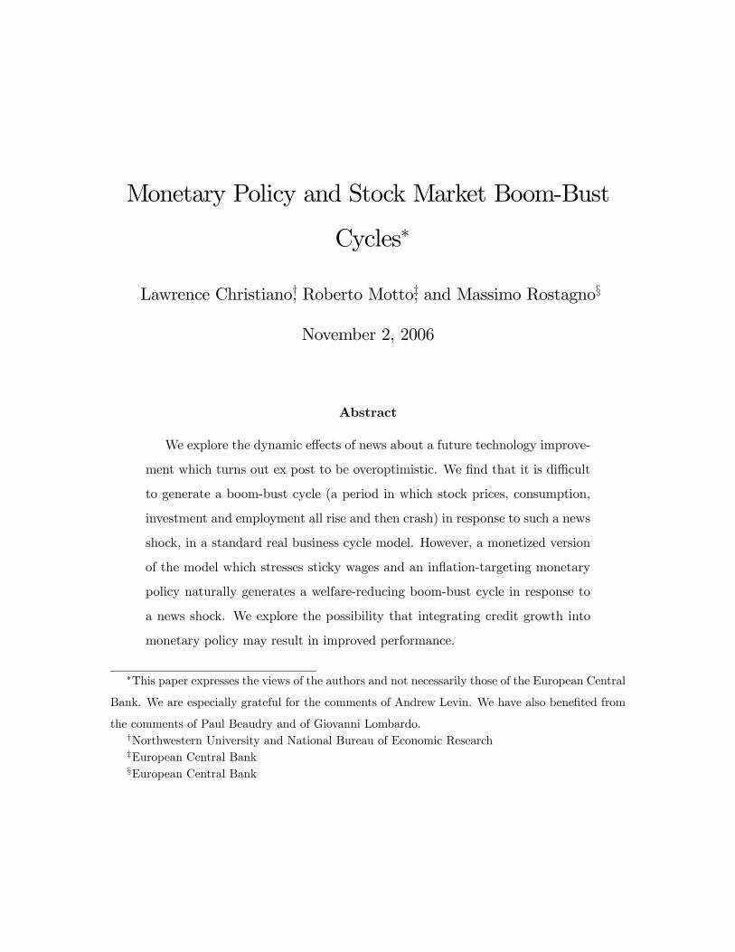
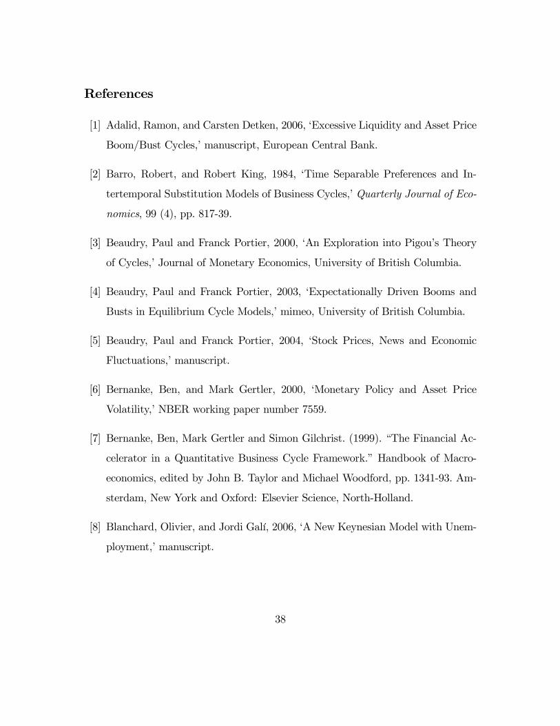
asset markets. A look at the data reveals the reason. Figure 1 displays monthly

observations on the S&P500 (converted into real terms using the CPI) for the period

1870 to early 2006. Note the recent dramatic boom and bust. Two other pronounced

“boom-bust” episodes are evident: the one that begins in the early 1920s and busts

near the start of the Great Depression, and another one that begins in the mid

1950s and busts in the 1970s. These observations raise several questions. What are

the basic forces driving the boom-bust episodes? Are they driven by economic fun-

damentals, or are they bubbles? The boom phase is associated with strong output,

employment, consumption and investment, while there is substantial economic weak-

ness (in one case, the biggest recorded recession in US history) in the bust phase.

Does this association reflect causality going from volatility in the stock market to

the real economy, or does causality go the other way? Or, is it that both are the

outcome of some other factor, perhaps the nature of monetary policy? The analysis

of this paper lends support to the latter hypothesis.

We study models that have been useful in the analysis of US and Euro Area busi-

ness cycles. We adopt the fundamentals perspective on boom-busts suggested by the

work of Beaudry and Portier (2000,2003,2004) and recently extended in the analysis

of Jaimovich and Rebelo (2006). The idea is that the boom phase is triggered by a

signal which leads agents to rationally expect an improvement in technology in the

future. Although the signal agents see is informative, it is not perfect. Occasionally,

the signal turns out to be false and the bust phase of the cycle begins when people

find this out. As an example, we have in mind the signals that led firms to invest

2

heavily in fiber-optic cable, only to be disappointed later by low profits. Another

example is the signals that led Motorola to launch satellites into orbit in the ex-

pectation (later disappointed) that the satellites would be profitable as cell phone

usage expanded. Although our analysis is based on rational expectations, we suspect

that the same basic results would go through under other theories of how agents can

become optimistic in ways that turn out ex post to be exaggerated.

Our notion of what triggers a boom-bust cycle is very stylized: the signal occurs

on a particular date and people learn that it is exactly false on another particular

date. In more realistic scenarios, people form expectations based on an accumulation

of various signals. If people’s expectations are in fact overoptimistic, they come to

this realization only slowly and over time. Although the trigger of the boom-bust

cycle in our analysis is in some ways simplistic, it has the advantage of allowing us

to highlight a result that we think is likely to survive in more realistic settings.

Our results are as follows. We find that - within the confines of the set of models

we consider - it is hard to account for a boom-bust episode (an episode in which

consumption, investment, output, employment and the stock market all rise sharply

and then crash) in a model that abstracts from nominal frictions. However, when we

introduce an inflation targeting central bank and sticky nominal wages, a theory of

boom-busts emerges naturally. In our environment, inflation targeting suboptimally

converts what would otherwise be a small economic fluctuation into a major boom-

bust episode. In this sense, our analysis is consistent with the view that boom-bust

episodes are in large part caused by monetary policy.

In our model, we represent monetary policy by an empirically estimated Taylor

rule. Because that rule satisfies the Taylor principle, we refer to it loosely as an

‘inflation targeting’ rule. Inflation targeting has the powerful attraction of anchoring

expectations in New Keynesian models. However, our analysis suggests that there

3

are also costs. The analysis suggests that it is desirable to modify the standard

inflation targeting approach to monetary policy in favor of a policy that does not

promote boom-busts. In our model, boom-bust episodes are correlated with strong

credit growth. So, a policy which not only targets inflation, but also ‘leans against

the wind’ by tightening monetary policy when credit growth is strong would reduce

some of the costs associated with pure inflation targeting.

Our results are based on model simulations, and so the credibility of the findings

depends on the plausibility of our model. For the purpose of our results here, the two

cornerstones of our model are sticky wages and an estimated Taylor rule. That the

latter is a reasonable way to capture monetary policy has almost become axiomatic.

Sticky wages have also emerged in recent years as a key feature of models that fit

the data well (see, for example, the discussion in Christiano, Eichenbaum and Evans

(2005).) The view that wage-setting frictions are key to understanding aggregate

fluctuations is also reached by a very different type of empirical analysis in Gali,

Gertler and Lopes-Salido (forthcoming).

That sticky wages and inflation targeting are uneasy bedfellows is easy to see.

When wages are sticky, an inflation targeting central bank in effect targets the real

wage. This produces inefficient outcomes when shocks occur which require an adjust-

ment to the real wage (Erceg, Henderson and Levin (2000).) For example, suppose

a shock - a positive oil price shock, say - occurs which reduces the value marginal

product of labor. Preventing a large fall in employment under these circumstances

would require a drop in the real wage. With sticky wages and an inflation-targeting

central bank, the required fall in the real wage would not occur and employment

would be inefficiently low.

That sticky wages and inflation targeting can cause the economy’s response to

an oil shock to be inefficient is well known. What is less well known is that the

4

interaction of sticky wages and inflation targeting in the form of a standard Taylor

rule can trigger a boom-bust episode. The logic is simple. In our model, when

agents receive a signal of improved future technology it is efficient for investment,

consumption and employment to all rise a little, and then fall when expectations

are disappointed. In the efficient allocations, the size of the boom is sharply limited

by the rise in the real wage that occurs as the shadow cost of labor increases with

higher work effort.1 When there are frictions in setting nominal wages, however, a

rise in the real wage requires that inflation be allowed to drift down. The inflation

targeting central bank, seeing this drift down in inflation, cuts the interest rate to

keep inflation on target. In our model, this cut in the interest rate triggers a credit

boom and makes the economic expansion much bigger than is socially optimal. In a

situation like this, a central bank that ‘leans against the wind’ when credit expands

sharply would raise welfare by reducing the magnitude of the boom-bust cycle.

The notion that inflation targeting increases the likelihood of stock market boom-

bust episodes contradicts conventional wisdom. We take it that the conventional

wisdom is defined by the work of Bernanke and Gertler (2000), who argue that

an inflation-targeting monetary authority automatically stabilizes the stock market.

The reason for this is that in the Bernanke-Gertler environment, inflation tends to

rise in a stock market boom, so that an inflation targeter would raise interest rates,

moderating the rise in stock prices.

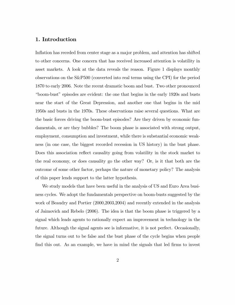
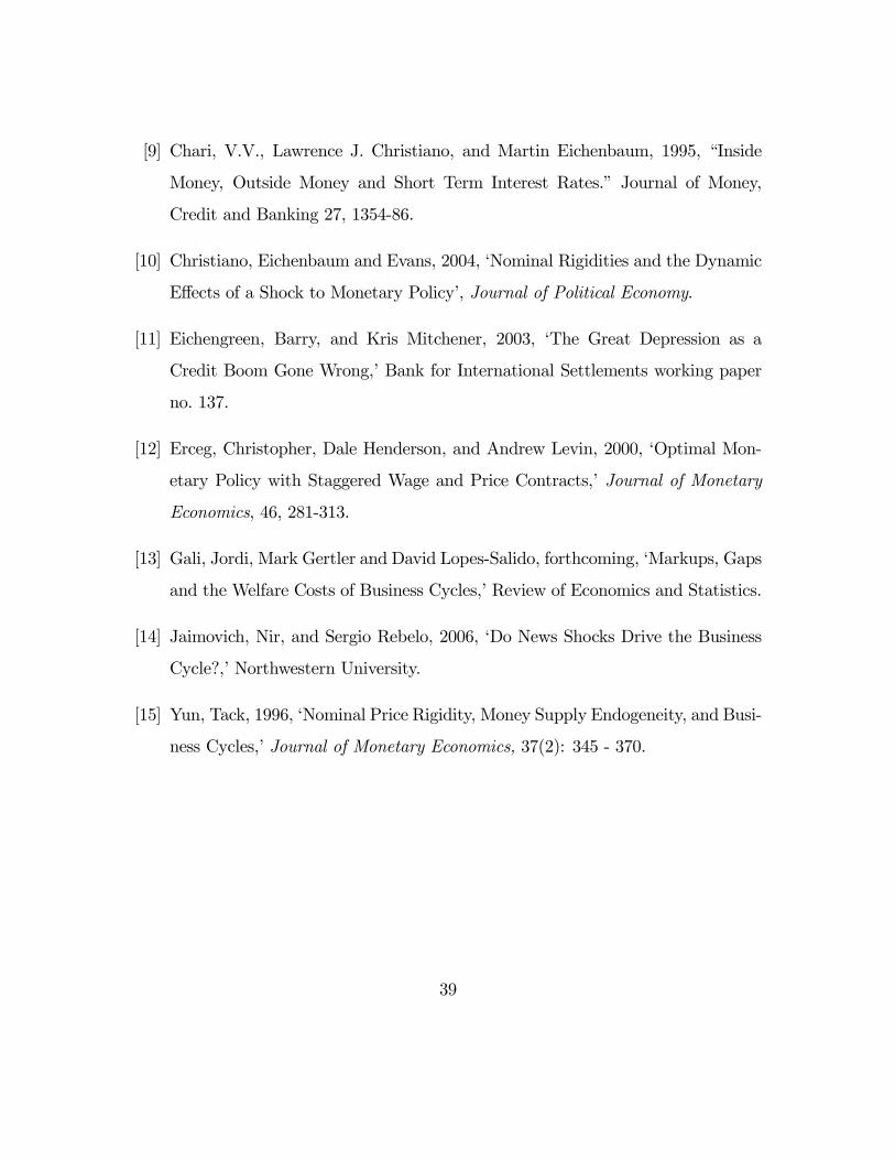
So, the behavior of inflation in the boom phase of a boom-bust cycle is the cru-

cial factor that distinguishes our story from the conventional wisdom. To assess the

two perspectives, consider Figure 2, which displays inflation and the stock market

in the three major US boom-bust episodes in the 20th century. In each case, in-

1Our definition of the ‘efficient allocations’ is conventional. They are the allocations that solve

the Ramsey problem.

5

flation is either falling or at least not rising during the initial phase of the boom.

Additional evidence is presented in Adalid and Detken (2006). They identify asset

price boom/bust episodes in 18 OECD countries since the 1970s. In their Table A1,

they show that inflation is on average weak during the boom-phase of these episodes.

In sum, the proposition that inflation is weak during the boom phase of boom-bust

cycles receives support from US and OECD data.

So far, we have stressed that integrating nominal variables and inflation targeting

into the analysis is merely helpful for understanding boom-bust episodes. In fact, if

one is not to wander too far from current standard models, it is essential.

To clarify this point, it is useful to think of the standard real business cycle model

that emerges when we strip away all monetary factors from our model. If we take a

completely standard version of such a model, a signal shock is completely incapable

of generating a boom-bust that resembles anything like what we see. Households in

effect react to the signal by going on vacation: consumption jumps, work goes down

and investment falls. When households realize the expected shock will not occur

they in effect find themselves in a situation with a low initial capital stock. The

dynamic response to this is familiar: they increase employment and investment and

reduce consumption. We identify the price of equity in the data with the price of

capital in the model. In the simplest version of the real business cycle model this is

fixed by technology at unity, so we have no movements in the stock prices. It is hard

to imagine a less successful model of a boom-bust cycle!

We then add habit persistence and costs of adjusting the flow of investment

(these are two features that have been found useful for understanding postwar busi-

ness cycles) and find that we make substantial progress towards a successful model.

However, this model also has a major failing that initially came to us as a surprise: in

the boom phase of the cycle, stock prices in the model fall and in the bust phase they

6

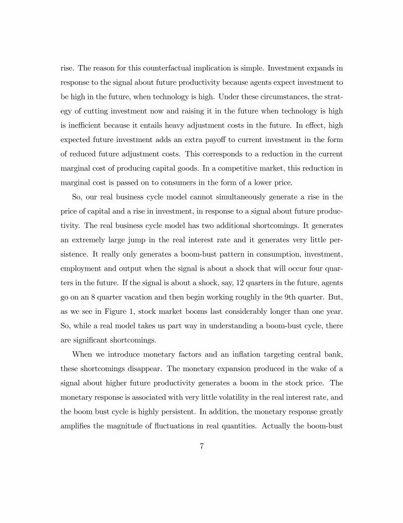
rise. The reason for this counterfactual implication is simple. Investment expands in

response to the signal about future productivity because agents expect investment to

be high in the future, when technology is high. Under these circumstances, the strat-

egy of cutting investment now and raising it in the future when technology is high

is inefficient because it entails heavy adjustment costs in the future. In effect, high

expected future investment adds an extra payoff to current investment in the form

of reduced future adjustment costs. This corresponds to a reduction in the current

marginal cost of producing capital goods. In a competitive market, this reduction in

marginal cost is passed on to consumers in the form of a lower price.

So, our real business cycle model cannot simultaneously generate a rise in the

price of capital and a rise in investment, in response to a signal about future produc-

tivity. The real business cycle model has two additional shortcomings. It generates

an extremely large jump in the real interest rate and it generates very little per-

sistence. It really only generates a boom-bust pattern in consumption, investment,

employment and output when the signal is about a shock that will occur four quar-

ters in the future. If the signal is about a shock, say, 12 quarters in the future, agents

go on an 8 quarter vacation and then begin working roughly in the 9th quarter. But,

as we see in Figure 1, stock market booms last considerably longer than one year.

So, while a real model takes us part way in understanding a boom-bust cycle, there

are significant shortcomings.

When we introduce monetary factors and an inflation targeting central bank,

these shortcomings disappear. The monetary expansion produced in the wake of a

signal about higher future productivity generates a boom in the stock price. The

monetary response is associated with very little volatility in the real interest rate, and

the boom bust cycle is highly persistent. In addition, the monetary response greatly

amplifies the magnitude of fluctuations in real quantities. Actually the boom-bust

7

produced in the monetary model is so much larger than it is in the real business cycle

model that it is not an exaggeration to say that our boom-bust episode is primarily

a monetary phenomenon.

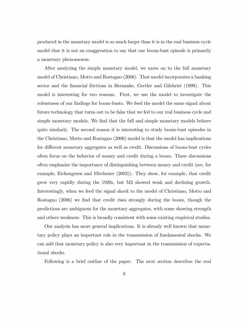
After analyzing the simple monetary model, we move on to the full monetary

model of Christiano, Motto and Rostagno (2006). That model incorporates a banking

sector and the financial frictions in Bernanke, Gertler and Gilchrist (1999). This

model is interesting for two reasons. First, we use the model to investigate the

robustness of our findings for boom-busts. We feed the model the same signal about

future technology that turns out to be false that we fed to our real business cycle and

simple monetary models. We find that the full and simple monetary models behave

quite similarly. The second reason it is interesting to study boom-bust episodes in

the Christiano, Motto and Rostagno (2006) model is that the model has implications

for different monetary aggregates as well as credit. Discussions of boom-bust cycles

often focus on the behavior of money and credit during a boom. These discussions

often emphasize the importance of distinguishing between money and credit (see, for

example, Eichengreen and Mitchener (2003)). They show, for example, that credit

grew very rapidly during the 1920s, but M2 showed weak and declining growth.

Interestingly, when we feed the signal shock to the model of Christiano, Motto and

Rostagno (2006) we find that credit rises strongly during the boom, though the

predictions are ambiguous for the monetary aggregates, with some showing strength

and others weakness. This is broadly consistent with some existing empirical studies.

Our analysis has more general implications. It is already well known that mone-

tary policy plays an important role in the transmission of fundamental shocks. We

can add that monetary policy is also very important in the transmission of expecta-

tional shocks.

Following is a brief outline of the paper. The next section describes the real

8

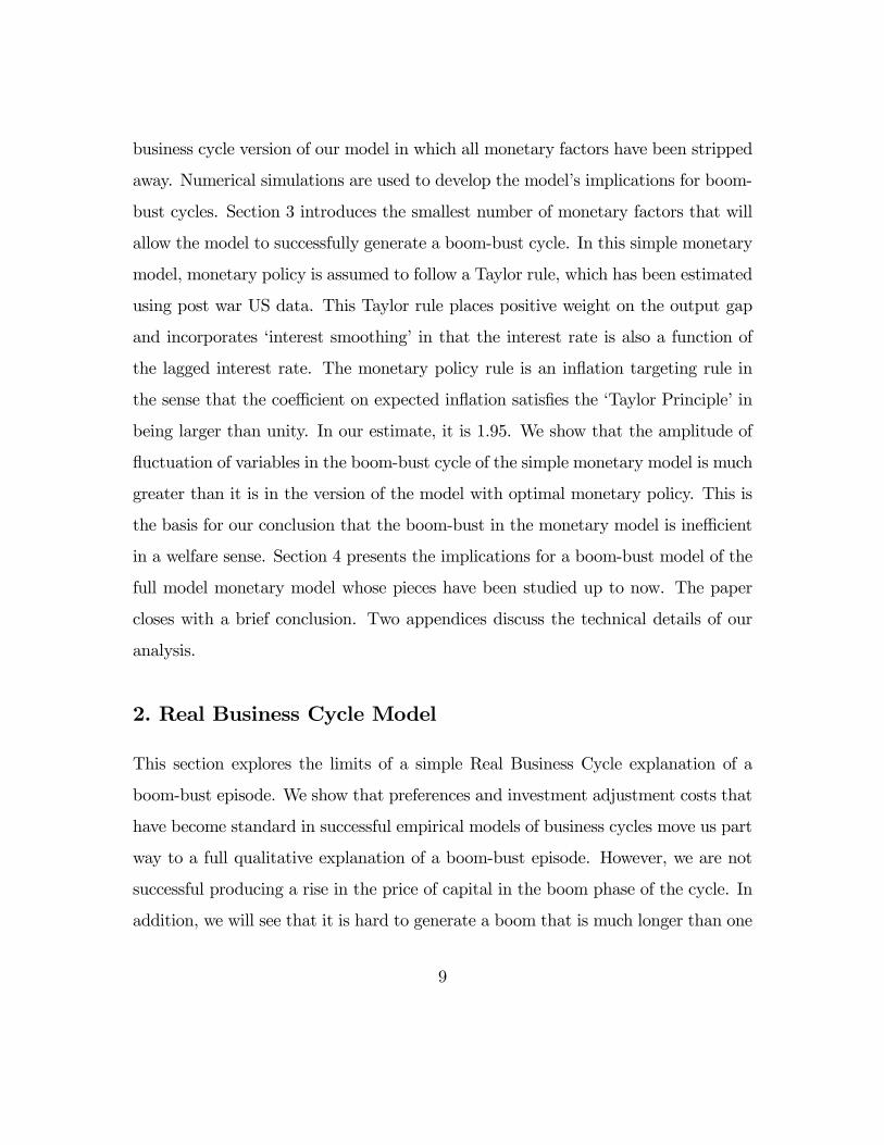
business cycle version of our model in which all monetary factors have been stripped

away. Numerical simulations are used to develop the model’s implications for boom-

bust cycles. Section 3 introduces the smallest number of monetary factors that will

allow the model to successfully generate a boom-bust cycle. In this simple monetary

model, monetary policy is assumed to follow a Taylor rule, which has been estimated

using post war US data. This Taylor rule places positive weight on the output gap

and incorporates ‘interest smoothing’ in that the interest rate is also a function of

the lagged interest rate. The monetary policy rule is an inflation targeting rule in

the sense that the coefficient on expected inflation satisfies the ‘Taylor Principle’ in

being larger than unity. In our estimate, it is 1.95. We show that the amplitude of

fluctuation of variables in the boom-bust cycle of the simple monetary model is much

greater than it is in the version of the model with optimal monetary policy. This is

the basis for our conclusion that the boom-bust in the monetary model is inefficient

in a welfare sense. Section 4 presents the implications for a boom-bust model of the

full model monetary model whose pieces have been studied up to now. The paper

closes with a brief conclusion. Two appendices discuss the technical details of our

analysis.

2. Real Business Cycle Model

This section explores the limits of a simple Real Business Cycle explanation of a

boom-bust episode. We show that preferences and investment adjustment costs that

have become standard in successful empirical models of business cycles move us part

way to a full qualitative explanation of a boom-bust episode. However, we are not

successful producing a rise in the price of capital in the boom phase of the cycle. In

addition, we will see that it is hard to generate a boom that is much longer than one

9

year. Finally, we will see that the model generates extreme fluctuations in the real

rate of interest.

2.1. The Model

The preferences of the representative household are given by:

Et

∞Xl=0

βl−t{log(Ct+l − bCt+l−1)− ψL

h1+σLt

1 + σL}

Here, ht is hours worked, Ct is consumption and the amount of time that is available

is unity. When b > 0 then there is habit persistence in preferences. The resource

constraint is

It + Ct ≤ Yt, (2.1)

where It is investment, Ct is consumption and Yt is output of goods.

Output Yt is produced using the technology

Yt = tKαt (ztht)

1−α , (2.2)

where t represents a stochastic shock to technology and zt follows a deterministic

growth path,

zt = zt−1 exp (µz) . (2.3)

The law of motion of t will be described shortly.

We consider two specifications of adjustment costs in investment. According to

one, adjustment costs are in terms of the change in the flow of investment:

Kt+1 = (1− δ)Kt + (1− S

µItIt−1

¶)It, (2.4)

where

S (x) =a

2(x− exp (µz))2 ,

10

with a > 0. We refer to this specification of adjustment costs as the ‘flow specifica-

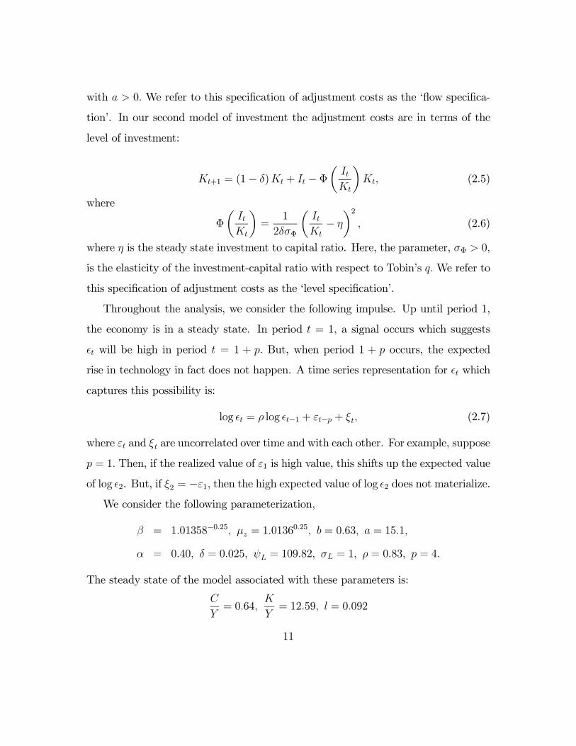
tion’. In our second model of investment the adjustment costs are in terms of the

level of investment:

Kt+1 = (1− δ)Kt + It − Φ

µItKt

¶Kt, (2.5)

where

Φ

µItKt

¶=

1

2δσΦ

µItKt− η

¶2, (2.6)

where η is the steady state investment to capital ratio. Here, the parameter, σΦ > 0,

is the elasticity of the investment-capital ratio with respect to Tobin’s q.We refer to

this specification of adjustment costs as the ‘level specification’.

Throughout the analysis, we consider the following impulse. Up until period 1,

the economy is in a steady state. In period t = 1, a signal occurs which suggests

t will be high in period t = 1 + p. But, when period 1 + p occurs, the expected

rise in technology in fact does not happen. A time series representation for t which

captures this possibility is:

log t = ρ log t−1 + εt−p + ξt, (2.7)

where εt and ξt are uncorrelated over time and with each other. For example, suppose

p = 1. Then, if the realized value of ε1 is high value, this shifts up the expected value

of log 2. But, if ξ2 = −ε1, then the high expected value of log 2 does not materialize.

We consider the following parameterization,

β = 1.01358−0.25, µz = 1.01360.25, b = 0.63, a = 15.1,

α = 0.40, δ = 0.025, ψL = 109.82, σL = 1, ρ = 0.83, p = 4.

The steady state of the model associated with these parameters is:

C

Y= 0.64,

K

Y= 12.59, l = 0.092

11

We interpret the time unit of the model as being one quarter. This model is a special

case of the model estimated in Christiano, Motto and Rostagno (2006) using US data.

In the above list, the parameters a and ρ were estimated; µz was estimated based

on the average growth rate of output; β was selected so that given µz the model

matches the average real return on three-month Treasury bills; σL was simply set to

produce a Frish labor supply of unity; b was taken from Christiano, Eichenbaum and

Evans (2004); α and δ were chosen to allow the model to match several ratios (see

Christiano, Motto and Rostagno (2006)).

2.2. Results

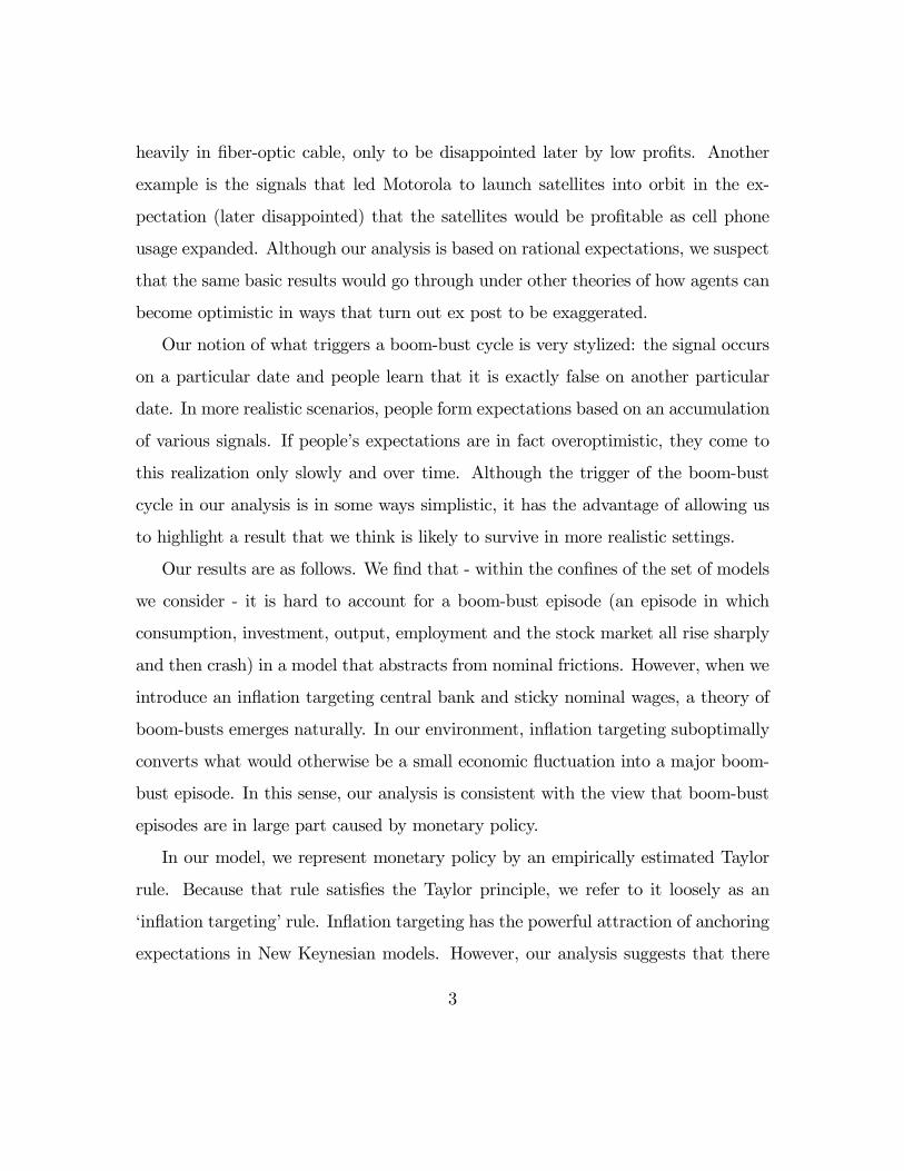
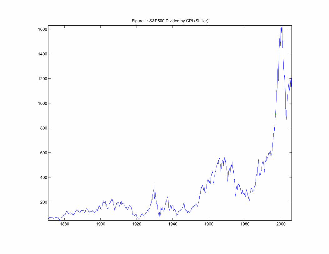
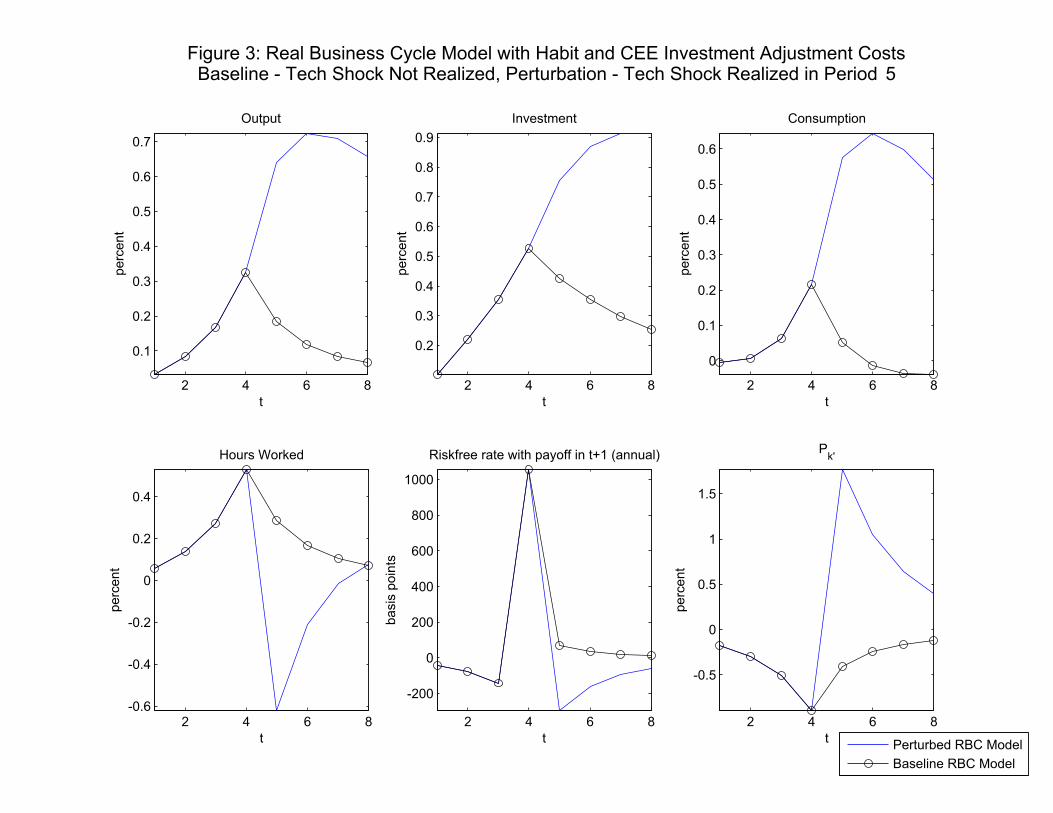
Consider the line with circles in Figure 3. This line displays the response of the

‘Baseline RBC’ model to a signal in period 1 that technology will jump in period 5

by 1 percent. Then, ξ5 = −0.01, so that the impact of the signal on t is cancelled

and no change ever happens to actual technology. Note how in the figure output,

investment and hours worked all rise until period 4 and then slowly decline. The

price of capital falls despite the anticipated rise in the payoff associated with capital.

This fall is discussed in further detail below, although perhaps it is not surprising

in view of the spike in the interest rate on one period consumption loans taken in

period 4. This jump in the interest rate is extraordinarily large. In the period before

the anticipated jump in technology, the real rate jumps by more than 10 percentage

points, at an annual rate.

The solid line in Figure 3 and the results in Figures 5-8 allow us to diagnose the

economics underlying the line with circles in Figure 3. In Figures 5-8, the circled

line in Figure 3 is reproduced for comparison. The solid line in Figure 3 displays

the response of the variables in the case when the technology shock is realized. This

12

shows the scenario which agents expect when they see the signal in period 1. Their

response has several interesting features. First, the rise in investment in period 4, the

first period in which investment can benefit from the higher expected rate of return,

is not especially larger than the rise in other periods, such as period 5. We suspect

that the failure of investment to rise more in period 4 reflects the consumption

smoothing motive. Period 4 is a period of relatively low productivity, and while

high investment then would benefit from the high period 5 rate of return, raising

investment in period 4 is costly in terms of consumption. The very high period 4

real interest rate is an indicator of just how costly consumption then is. Second,

hours worked drops sharply in the period when the technology shock is realized. The

drop in employment in our simulation reflects the importance of the wealth effect

on labor. This wealth effect is not felt in periods before 5 because of high interest

rate before then. Commenting on an earlier draft of our work, Jaimovich and Rebelo

(2006) conjecture that this drop is counterfactual, and they propose an alternative

specification of utility in which it does not occur. An alternative possibility is that

the sharp movement in employment reflects the absence of labor market frictions in

our model. For example, we suspect that if we incorporate a simple model of labor

search frictions the drop in employment will be greatly attenuated while the basic

message of the paper will be unaffected (see Blanchard and Gali (2006)).

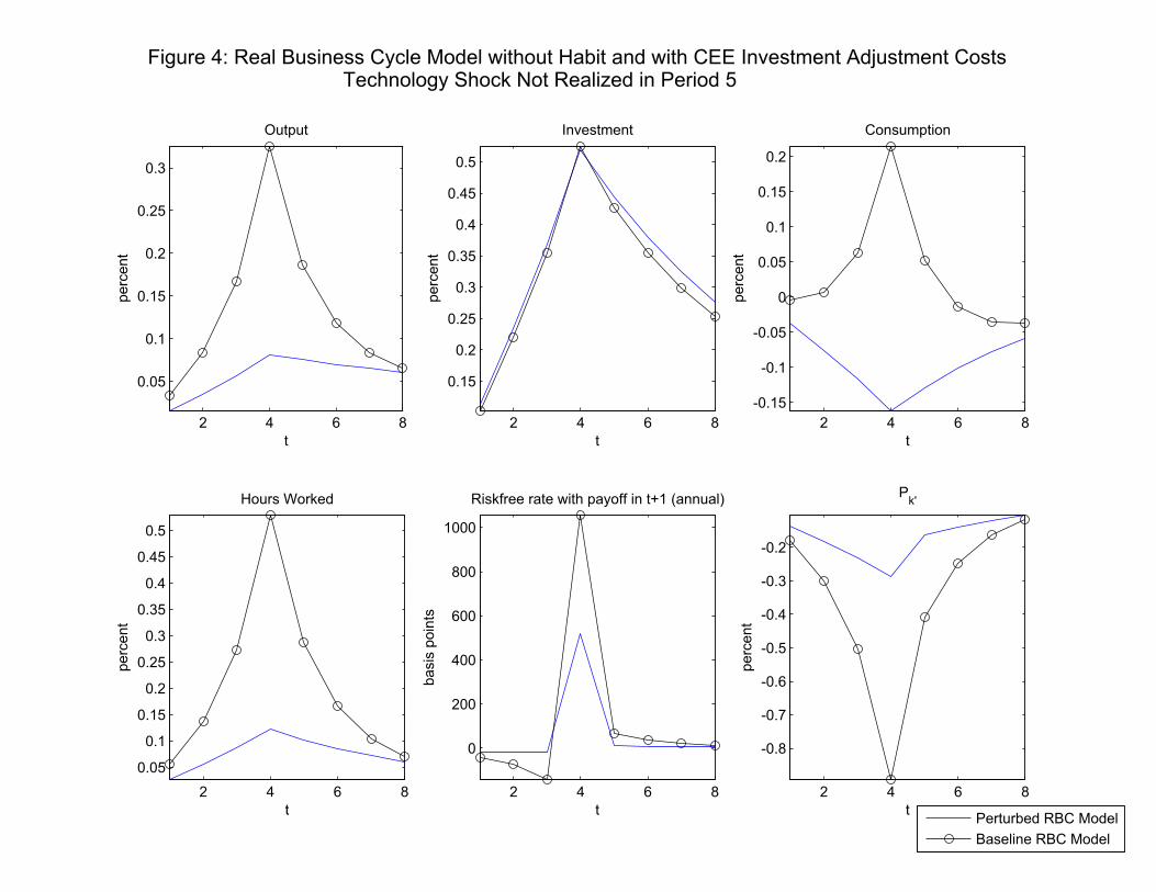
Figure 4 allows us to assess the role of habit persistence in the responses in Figure

3. Three things are worth emphasizing based on this figure. First, Figure 4 shows

that b > 0 is a key reason why consumption rises in periods before period 5 in Figure

3. Households, understanding that in period 5 they will want to consume at a high

level, experience a jump in the marginal utility of consumption in earlier periods

because of habit persistence. This can be seen in the expression for the marginal

13

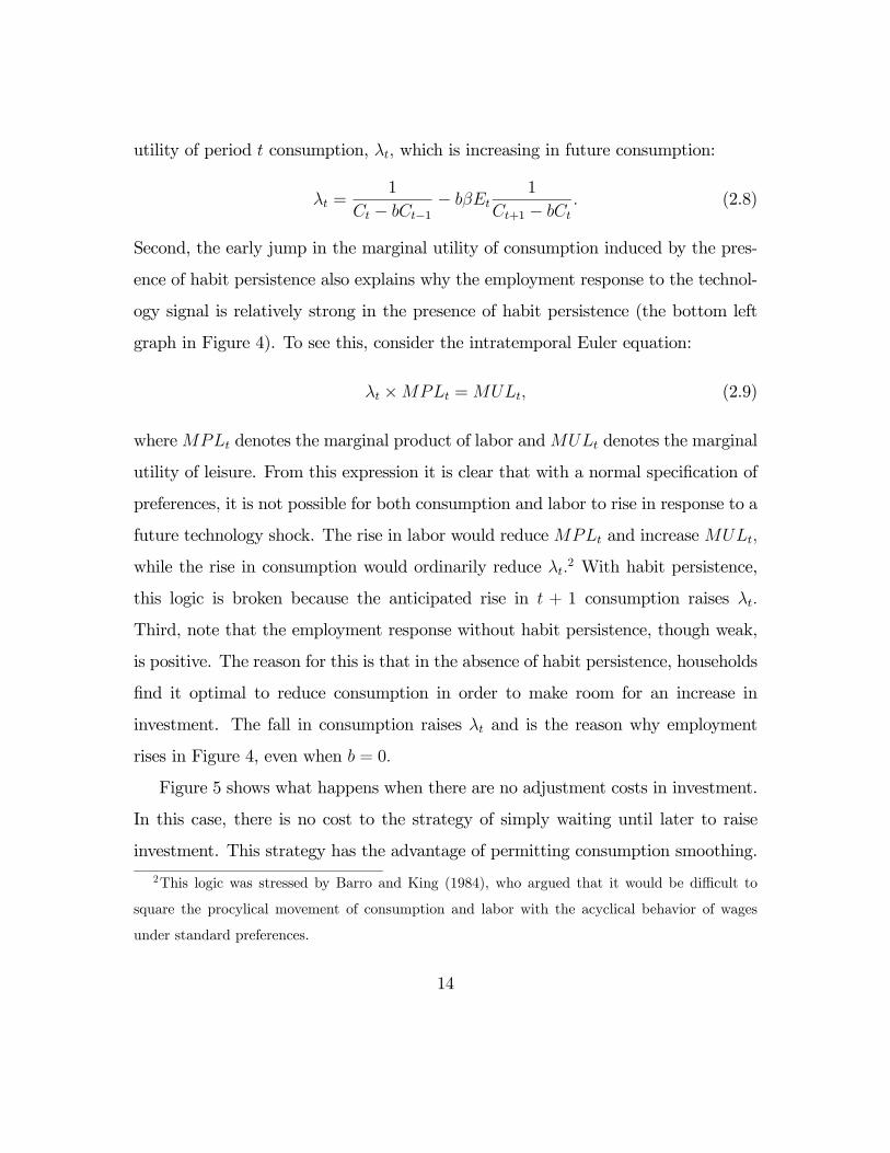
utility of period t consumption, λt, which is increasing in future consumption:

λt =1

Ct − bCt−1− bβEt

1

Ct+1 − bCt. (2.8)

Second, the early jump in the marginal utility of consumption induced by the pres-

ence of habit persistence also explains why the employment response to the technol-

ogy signal is relatively strong in the presence of habit persistence (the bottom left

graph in Figure 4). To see this, consider the intratemporal Euler equation:

λt ×MPLt =MULt, (2.9)

whereMPLt denotes the marginal product of labor andMULt denotes the marginal

utility of leisure. From this expression it is clear that with a normal specification of

preferences, it is not possible for both consumption and labor to rise in response to a

future technology shock. The rise in labor would reduce MPLt and increase MULt,

while the rise in consumption would ordinarily reduce λt.2 With habit persistence,

this logic is broken because the anticipated rise in t + 1 consumption raises λt.

Third, note that the employment response without habit persistence, though weak,

is positive. The reason for this is that in the absence of habit persistence, households

find it optimal to reduce consumption in order to make room for an increase in

investment. The fall in consumption raises λt and is the reason why employment

rises in Figure 4, even when b = 0.

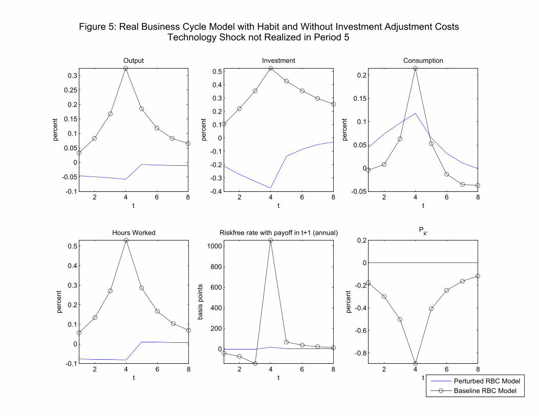
Figure 5 shows what happens when there are no adjustment costs in investment.

In this case, there is no cost to the strategy of simply waiting until later to raise

investment. This strategy has the advantage of permitting consumption smoothing.

2This logic was stressed by Barro and King (1984), who argued that it would be difficult to

square the procylical movement of consumption and labor with the acyclical behavior of wages

under standard preferences.

14

One way to see this is to note how the real rate of interest hardly moves when there

are no investment adjustment costs.

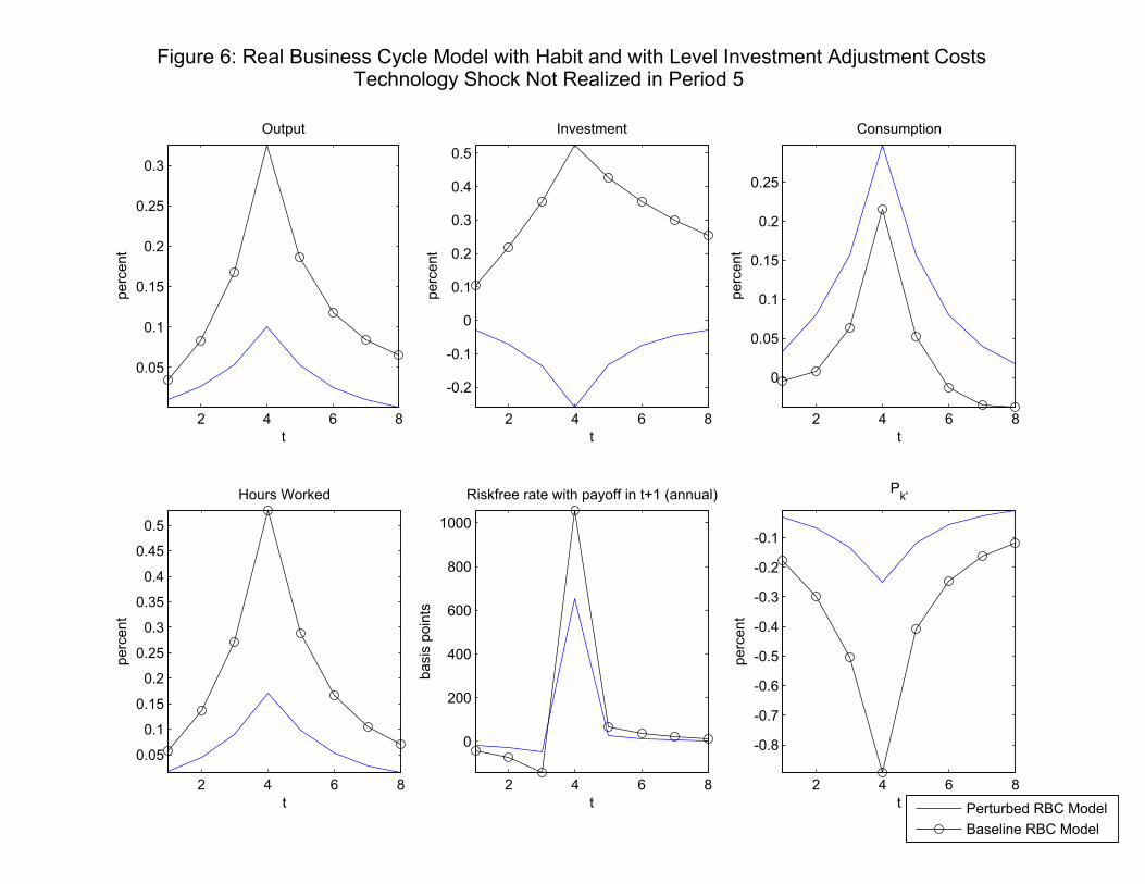
Figure 6 shows what happens when we adopt the level specification of adjustment

costs. With this specification, investment falls in response to the signal. This makes

room for additional consumption which reduces λt and accounts for the weak response

of employment after the signal (bottom left graph in Figure 6). So, Figure 6 indicates

that the flow specification of adjustment costs in our baseline real business cycle

model plays an important role in producing the responses in Figure 3.

A final experiment was motivated by the fact that in practice the boom phase

of a boom-bust cycle often lasts considerably more than 4 quarters. To investigate

whether the real business cycle model can generate a longer boom phase, we consid-

ered an example in which there is a period of 3 years from the date of the signal to

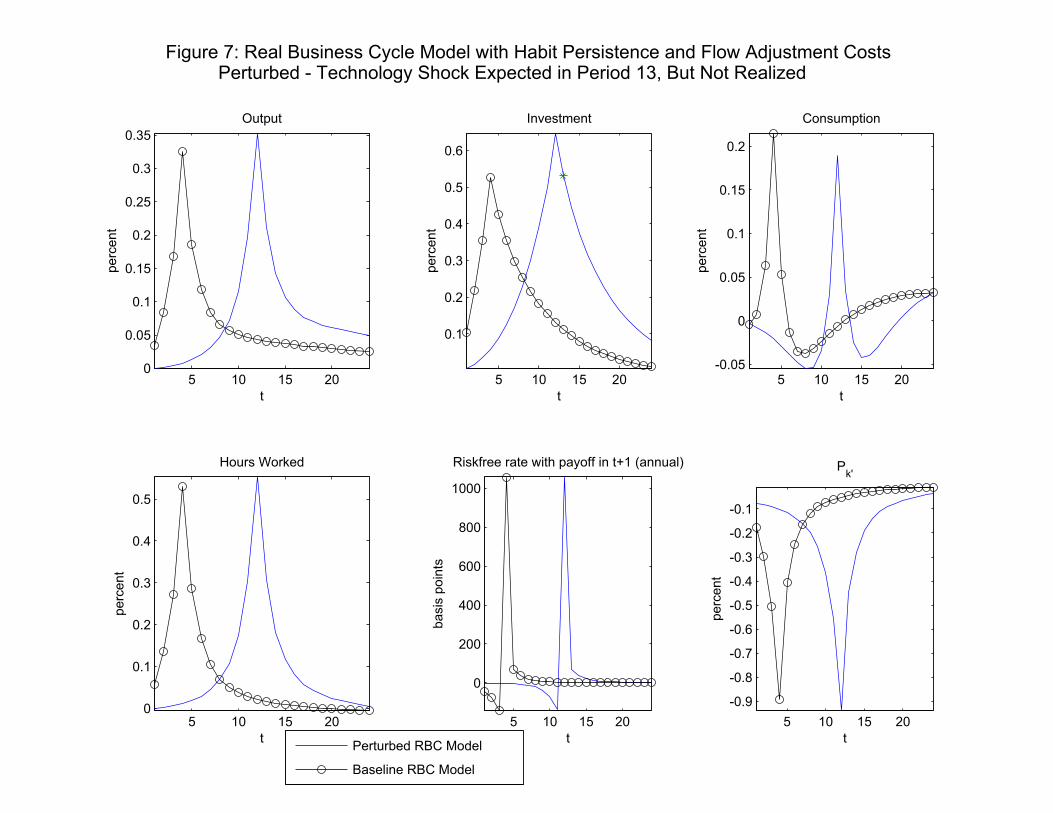
the bust. Figure 7 displays simulation results for the case when p = 12. Notice that

we have in fact not lengthened the boom phase very much because output, employ-

ment and investment actually only begin to rise about 4 quarters before the bust.

In addition, the model no longer generates a rise in consumption in response to the

signal. According to the figure, consumption falls (after a very brief rise) in the first

9 quarters. Evidently, households follow a strategy similar to the one in Figure 4,

when there is no habit. There, consumption falls in order to increase the resources

available for investment. Households with habit persistence do not mind following a

similar strategy as long as they can do so over a long enough period of time. With

time, habit stocks fall, thus mitigating the pain of reducing consumption.

15

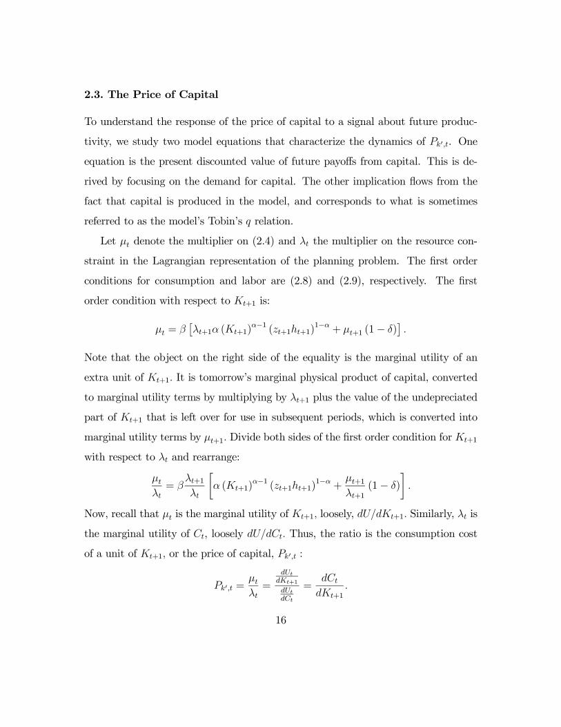
2.3. The Price of Capital

To understand the response of the price of capital to a signal about future produc-

tivity, we study two model equations that characterize the dynamics of Pk0,t. One

equation is the present discounted value of future payoffs from capital. This is de-

rived by focusing on the demand for capital. The other implication flows from the

fact that capital is produced in the model, and corresponds to what is sometimes

referred to as the model’s Tobin’s q relation.

Let µt denote the multiplier on (2.4) and λt the multiplier on the resource con-

straint in the Lagrangian representation of the planning problem. The first order

conditions for consumption and labor are (2.8) and (2.9), respectively. The first

order condition with respect to Kt+1 is:

µt = β£λt+1α (Kt+1)

α−1 (zt+1ht+1)1−α + µt+1 (1− δ)

¤.

Note that the object on the right side of the equality is the marginal utility of an

extra unit of Kt+1. It is tomorrow’s marginal physical product of capital, converted

to marginal utility terms by multiplying by λt+1 plus the value of the undepreciated

part of Kt+1 that is left over for use in subsequent periods, which is converted into

marginal utility terms by µt+1. Divide both sides of the first order condition for Kt+1

with respect to λt and rearrange:

µtλt= β

λt+1λt

∙α (Kt+1)

α−1 (zt+1ht+1)1−α +

µt+1λt+1

(1− δ)

¸.

Now, recall that µt is the marginal utility of Kt+1, loosely, dU/dKt+1. Similarly, λt is

the marginal utility of Ct, loosely dU/dCt. Thus, the ratio is the consumption cost

of a unit of Kt+1, or the price of capital, Pk0,t :

Pk0,t =µtλt=

dUtdKt+1

dUtdCt

=dCt

dKt+1.

16

Substituting this into the first order condition for Kt+1, we obtain:

Pk0,t = Etβλt+1λt

£rkt+1α+ Pk0,t+1 (1− δ)

¤,

where

rkt+1 = α (Kt+1)α−1 (zt+1ht+1)

1−α .

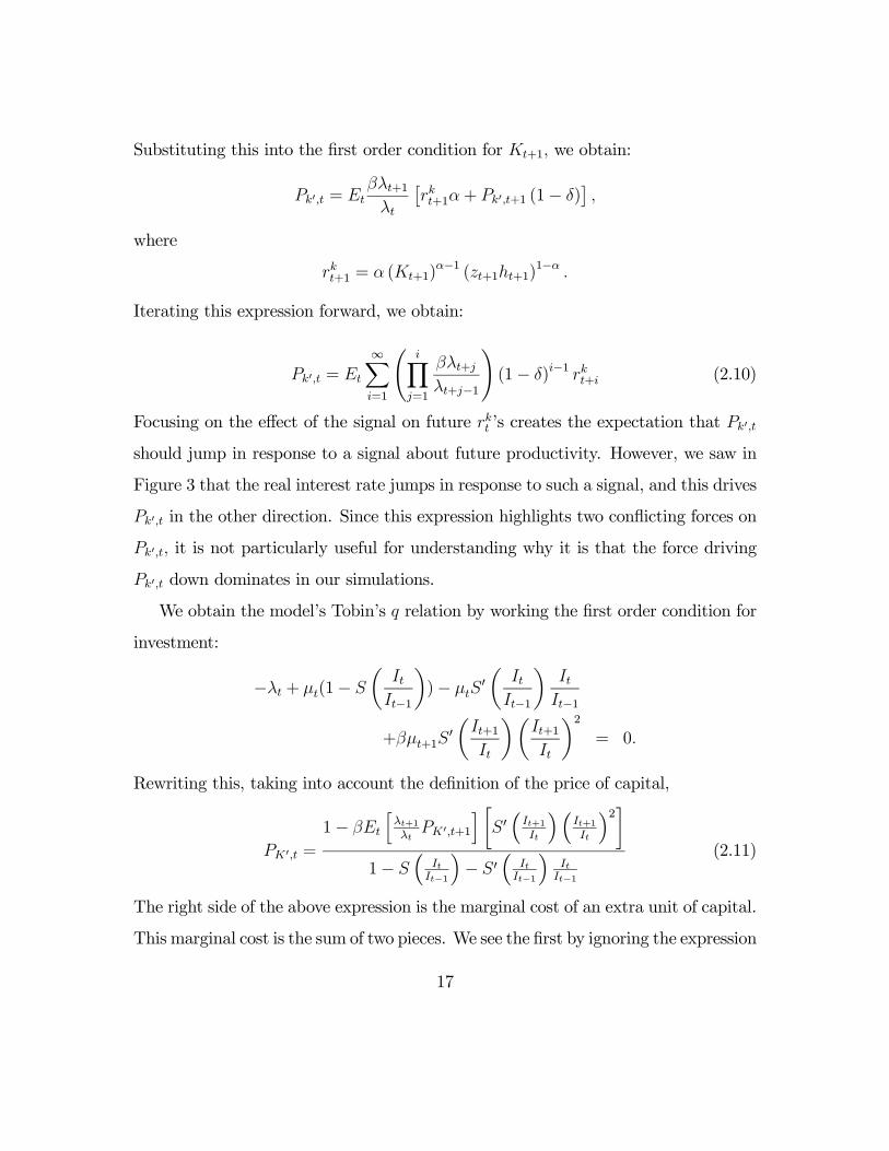
Iterating this expression forward, we obtain:

Pk0,t = Et

∞Xi=1

ÃiY

j=1

βλt+jλt+j−1

!(1− δ)i−1 rkt+i (2.10)

Focusing on the effect of the signal on future rkt ’s creates the expectation that Pk0,t

should jump in response to a signal about future productivity. However, we saw in

Figure 3 that the real interest rate jumps in response to such a signal, and this drives

Pk0,t in the other direction. Since this expression highlights two conflicting forces on

Pk0,t, it is not particularly useful for understanding why it is that the force driving

Pk0,t down dominates in our simulations.

We obtain the model’s Tobin’s q relation by working the first order condition for

investment:

−λt + µt(1− S

µItIt−1

¶)− µtS

0µ

ItIt−1

¶ItIt−1

+βµt+1S0µIt+1It

¶µIt+1It

¶2= 0.

Rewriting this, taking into account the definition of the price of capital,

PK0,t =

1− βEt

hλt+1λt

PK0,t+1

i ∙S0³It+1It

´³It+1It

´2¸1− S

³It

It−1

´− S0

³It

It−1

´It

It−1

(2.11)

The right side of the above expression is the marginal cost of an extra unit of capital.

This marginal cost is the sum of two pieces. We see the first by ignoring the expression

17

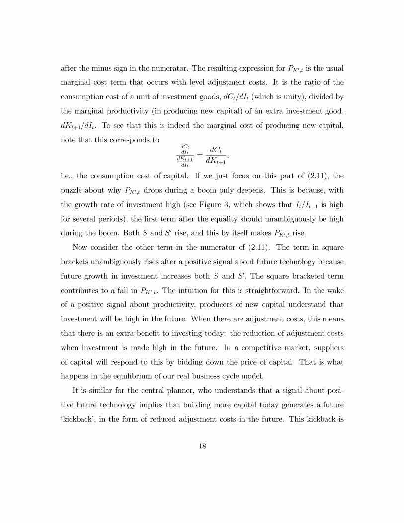
after the minus sign in the numerator. The resulting expression for PK0,t is the usual

marginal cost term that occurs with level adjustment costs. It is the ratio of the

consumption cost of a unit of investment goods, dCt/dIt (which is unity), divided by

the marginal productivity (in producing new capital) of an extra investment good,

dKt+1/dIt. To see that this is indeed the marginal cost of producing new capital,

note that this corresponds todCtdIt

dKt+1

dIt

=dCt

dKt+1,

i.e., the consumption cost of capital. If we just focus on this part of (2.11), the

puzzle about why PK0,t drops during a boom only deepens. This is because, with

the growth rate of investment high (see Figure 3, which shows that It/It−1 is high

for several periods), the first term after the equality should unambiguously be high

during the boom. Both S and S0 rise, and this by itself makes PK0,t rise.

Now consider the other term in the numerator of (2.11). The term in square

brackets unambiguously rises after a positive signal about future technology because

future growth in investment increases both S and S0. The square bracketed term

contributes to a fall in PK0,t. The intuition for this is straightforward. In the wake

of a positive signal about productivity, producers of new capital understand that

investment will be high in the future. When there are adjustment costs, this means

that there is an extra benefit to investing today: the reduction of adjustment costs

when investment is made high in the future. In a competitive market, suppliers

of capital will respond to this by bidding down the price of capital. That is what

happens in the equilibrium of our real business cycle model.

It is similar for the central planner, who understands that a signal about posi-

tive future technology implies that building more capital today generates a future

‘kickback’, in the form of reduced adjustment costs in the future. This kickback is

18

properly thought of as a reduction to the marginal cost of producing current capital,

and is fundamentally the reason the planner is motivated to increase current invest-

ment. This reasoning suggests to us that there will not be a simple perturbation

of the real business cycle model which will generate a rise in investment and a rise

in the price of capital after a signal about future technology. This motivates us to

consider the monetary version of the model in the next subsection.

3. Introducing Nominal Features and an Inflation-Targeting

Central Bank

We now modify our model to introduce monetary policy and wage/price frictions.

In the first subsection below, we present the model. In the second subsection we

present our numerical results.

3.1. Simple Monetary Model

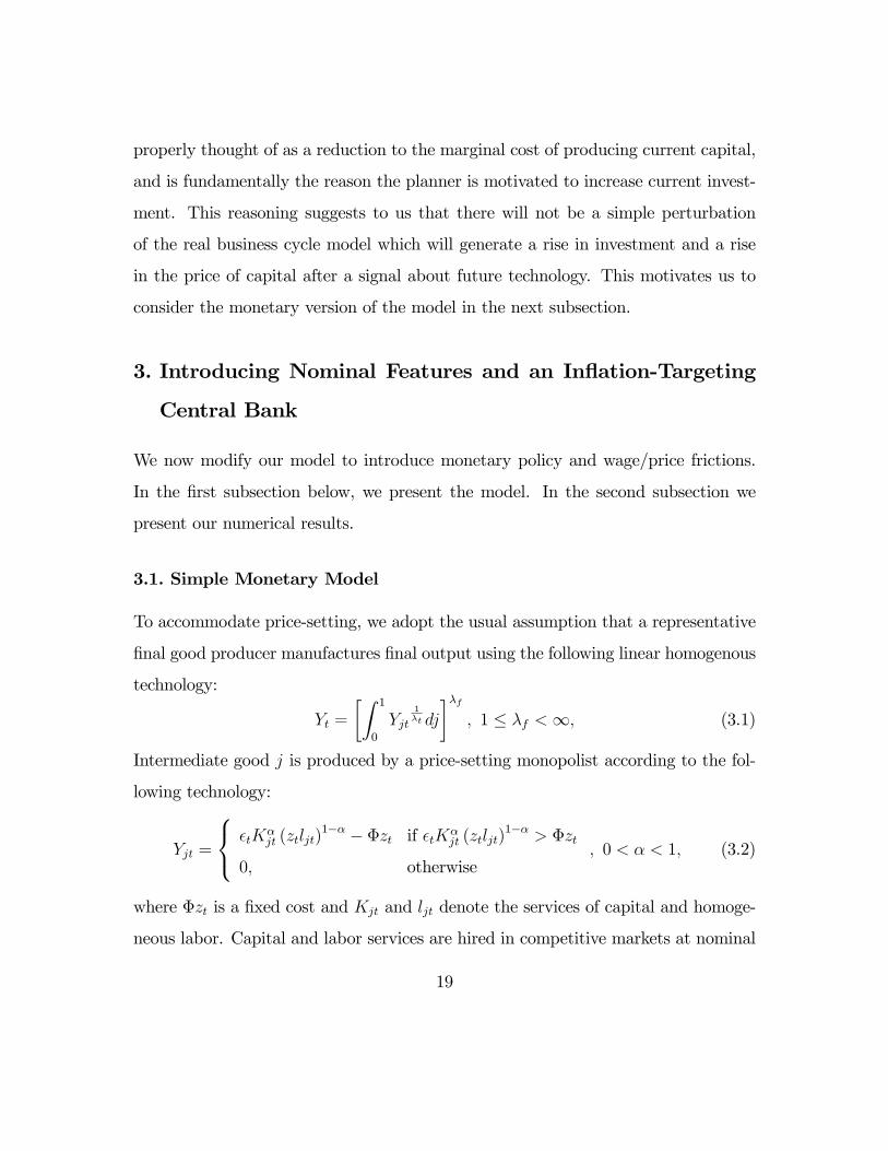
To accommodate price-setting, we adopt the usual assumption that a representative

final good producer manufactures final output using the following linear homogenous

technology:

Yt =

∙Z 1

0

Yjt1λt dj

¸λf, 1 ≤ λf <∞, (3.1)

Intermediate good j is produced by a price-setting monopolist according to the fol-

lowing technology:

Yjt =

⎧⎨⎩ tKαjt (ztljt)

1−α − Φzt if tKαjt (ztljt)

1−α > Φzt

0, otherwise, 0 < α < 1, (3.2)

where Φzt is a fixed cost and Kjt and ljt denote the services of capital and homoge-

neous labor. Capital and labor services are hired in competitive markets at nominal

19

prices, Ptrkt , and Wt, respectively.

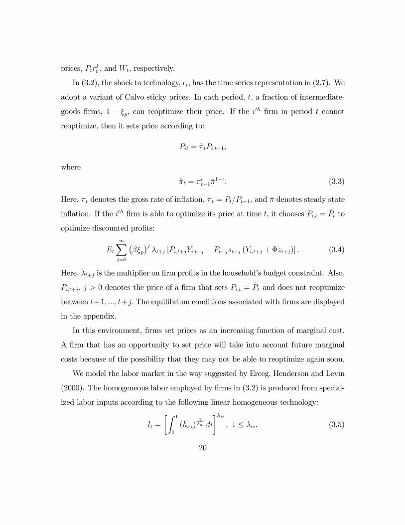
In (3.2), the shock to technology, t, has the time series representation in (2.7). We

adopt a variant of Calvo sticky prices. In each period, t, a fraction of intermediate-

goods firms, 1 − ξp, can reoptimize their price. If the ith firm in period t cannot

reoptimize, then it sets price according to:

Pit = π̃tPi,t−1,

where

π̃t = πιt−1π̄1−ι. (3.3)

Here, πt denotes the gross rate of inflation, πt = Pt/Pt−1, and π̄ denotes steady state

inflation. If the ith firm is able to optimize its price at time t, it chooses Pi,t = P̃t to

optimize discounted profits:

Et

∞Xj=0

¡βξp¢jλt+j [Pi,t+jYi,t+j − Pt+jst+j (Yi,t+j + Φzt+j)] . (3.4)

Here, λt+j is the multiplier on firm profits in the household’s budget constraint. Also,

Pi,t+j, j > 0 denotes the price of a firm that sets Pi,t = P̃t and does not reoptimize

between t+1, ..., t+j. The equilibrium conditions associated with firms are displayed

in the appendix.

In this environment, firms set prices as an increasing function of marginal cost.

A firm that has an opportunity to set price will take into account future marginal

costs because of the possibility that they may not be able to reoptimize again soon.

We model the labor market in the way suggested by Erceg, Henderson and Levin

(2000). The homogeneous labor employed by firms in (3.2) is produced from special-

ized labor inputs according to the following linear homogeneous technology:

lt =

∙Z 1

0

(ht,i)1λw di

¸λw, 1 ≤ λw. (3.5)

20

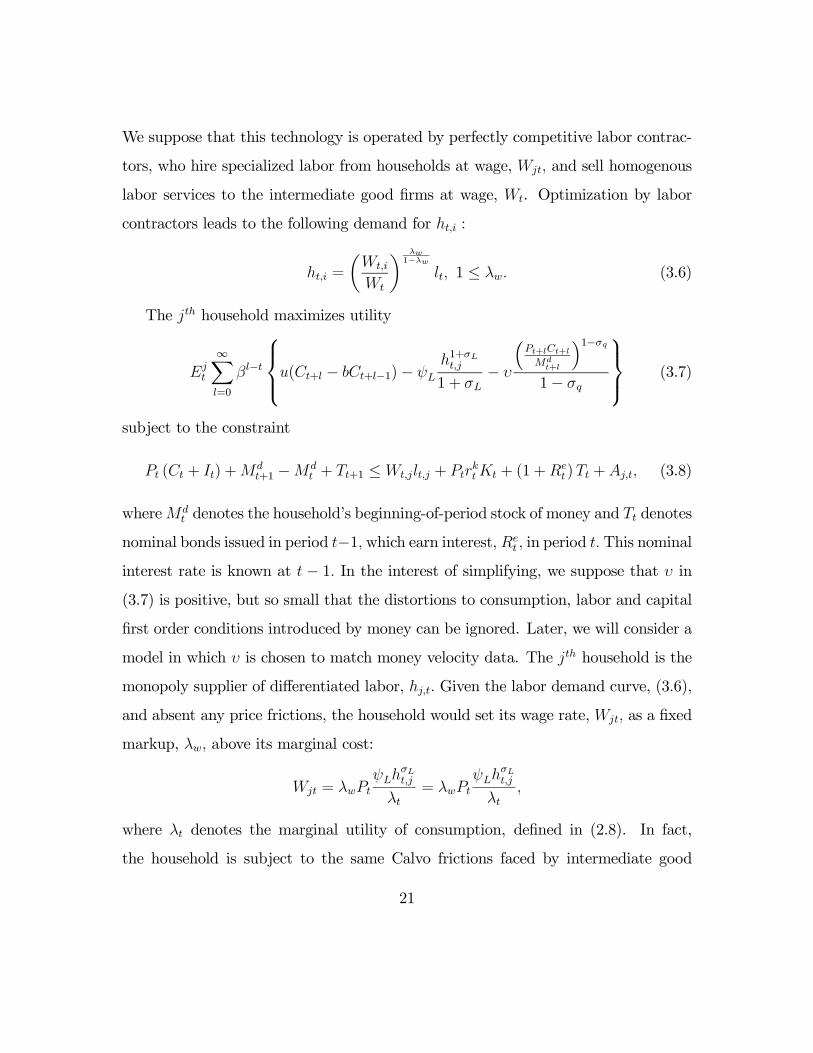
We suppose that this technology is operated by perfectly competitive labor contrac-

tors, who hire specialized labor from households at wage, Wjt, and sell homogenous

labor services to the intermediate good firms at wage, Wt. Optimization by labor

contractors leads to the following demand for ht,i :

ht,i =

µWt,i

Wt

¶ λw1−λw

lt, 1 ≤ λw. (3.6)

The jth household maximizes utility

Ejt

∞Xl=0

βl−t

⎧⎪⎨⎪⎩u(Ct+l − bCt+l−1)− ψL

h1+σLt,j

1 + σL− υ

³Pt+lCt+lMdt+l

´1−σq1− σq

⎫⎪⎬⎪⎭ (3.7)

subject to the constraint

Pt (Ct + It) +Mdt+1 −Md

t + Tt+1 ≤Wt,jlt,j + PtrktKt + (1 +Re

t )Tt +Aj,t, (3.8)

whereMdt denotes the household’s beginning-of-period stock of money and Tt denotes

nominal bonds issued in period t−1, which earn interest, Ret , in period t. This nominal

interest rate is known at t − 1. In the interest of simplifying, we suppose that υ in

(3.7) is positive, but so small that the distortions to consumption, labor and capital

first order conditions introduced by money can be ignored. Later, we will consider a

model in which υ is chosen to match money velocity data. The jth household is the

monopoly supplier of differentiated labor, hj,t. Given the labor demand curve, (3.6),

and absent any price frictions, the household would set its wage rate, Wjt, as a fixed

markup, λw, above its marginal cost:

Wjt = λwPt

ψLhσLt,j

λt= λwPt

ψLhσLt,j

λt,

where λt denotes the marginal utility of consumption, defined in (2.8). In fact,

the household is subject to the same Calvo frictions faced by intermediate good

21

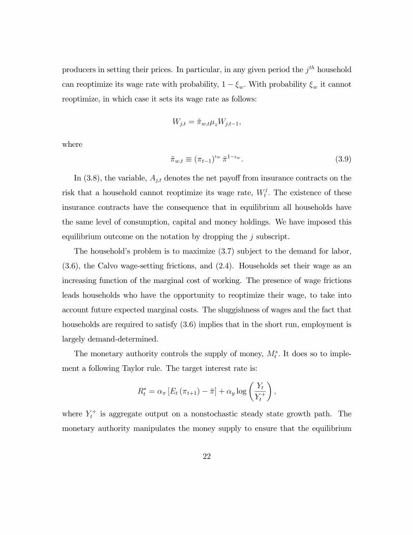
producers in setting their prices. In particular, in any given period the jth household

can reoptimize its wage rate with probability, 1− ξw. With probability ξw it cannot

reoptimize, in which case it sets its wage rate as follows:

Wj,t = π̃w,tµzWj,t−1,

where

π̃w,t ≡ (πt−1)ιw π̄1−ιw . (3.9)

In (3.8), the variable, Aj,t denotes the net payoff from insurance contracts on the

risk that a household cannot reoptimize its wage rate, W jt . The existence of these

insurance contracts have the consequence that in equilibrium all households have

the same level of consumption, capital and money holdings. We have imposed this

equilibrium outcome on the notation by dropping the j subscript.

The household’s problem is to maximize (3.7) subject to the demand for labor,

(3.6), the Calvo wage-setting frictions, and (2.4). Households set their wage as an

increasing function of the marginal cost of working. The presence of wage frictions

leads households who have the opportunity to reoptimize their wage, to take into

account future expected marginal costs. The sluggishness of wages and the fact that

households are required to satisfy (3.6) implies that in the short run, employment is

largely demand-determined.

The monetary authority controls the supply of money, M st . It does so to imple-

ment a following Taylor rule. The target interest rate is:

R∗t = απ [Et (πt+1)− π̄] + αy log

µYtY +t

¶,

where Y +t is aggregate output on a nonstochastic steady state growth path. The

monetary authority manipulates the money supply to ensure that the equilibrium

22

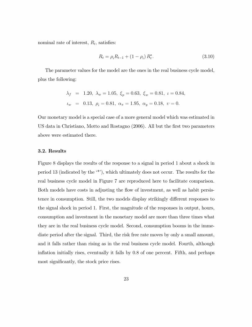
nominal rate of interest, Rt, satisfies:

Rt = ρiRt−1 + (1− ρi)R∗t . (3.10)

The parameter values for the model are the ones in the real business cycle model,

plus the following:

λf = 1.20, λw = 1.05, ξp = 0.63, ξw = 0.81, ι = 0.84,

ιw = 0.13, ρi = 0.81, απ = 1.95, αy = 0.18, υ = 0.

Our monetary model is a special case of a more general model which was estimated in

US data in Christiano, Motto and Rostagno (2006). All but the first two parameters

above were estimated there.

3.2. Results

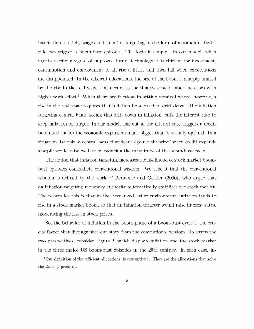
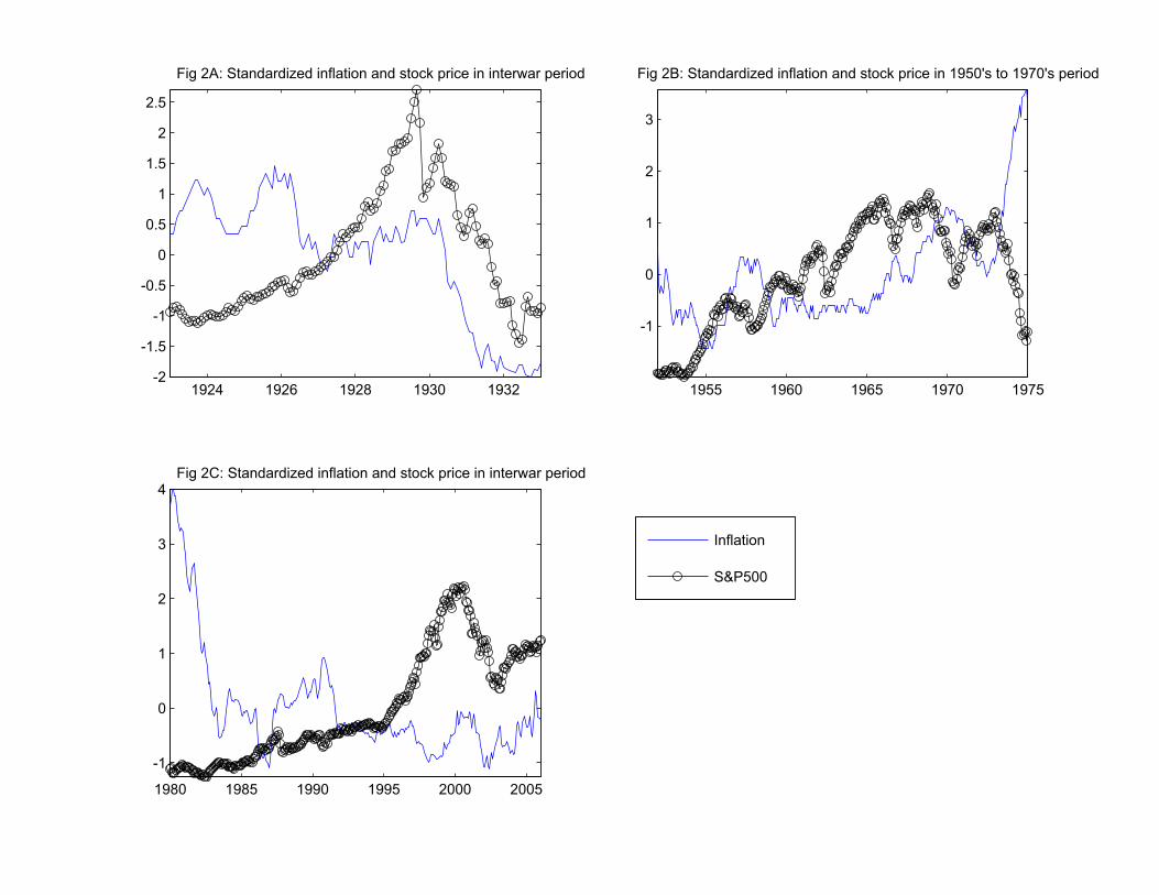
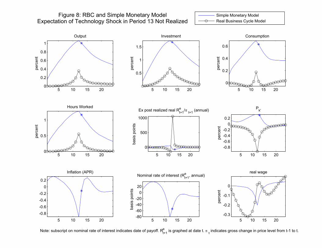
Figure 8 displays the results of the response to a signal in period 1 about a shock in

period 13 (indicated by the ‘*’), which ultimately does not occur. The results for the

real business cycle model in Figure 7 are reproduced here to facilitate comparison.

Both models have costs in adjusting the flow of investment, as well as habit persis-

tence in consumption. Still, the two models display strikingly different responses to

the signal shock in period 1. First, the magnitude of the responses in output, hours,

consumption and investment in the monetary model are more than three times what

they are in the real business cycle model. Second, consumption booms in the imme-

diate period after the signal. Third, the risk free rate moves by only a small amount,

and it falls rather than rising as in the real business cycle model. Fourth, although

inflation initially rises, eventually it falls by 0.8 of one percent. Fifth, and perhaps

most significantly, the stock price rises.

23

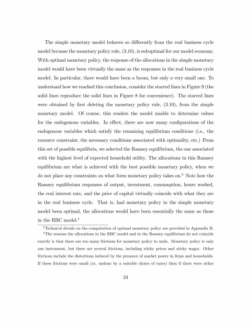
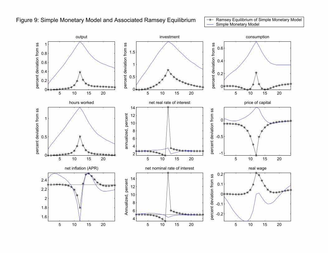
The simple monetary model behaves so differently from the real business cycle

model because the monetary policy rule, (3.10), is suboptimal for our model economy.

With optimal monetary policy, the response of the allocations in the simple monetary

model would have been virtually the same as the responses in the real business cycle

model. In particular, there would have been a boom, but only a very small one. To

understand how we reached this conclusion, consider the starred lines in Figure 9 (the

solid lines reproduce the solid lines in Figure 8 for convenience). The starred lines

were obtained by first deleting the monetary policy rule, (3.10), from the simple

monetary model. Of course, this renders the model unable to determine values

for the endogenous variables. In effect, there are now many configurations of the

endogenous variables which satisfy the remaining equilibrium conditions (i.e., the

resource constraint, the necessary conditions associated with optimality, etc.) From

this set of possible equilibria, we selected the Ramsey equilibrium, the one associated

with the highest level of expected household utility. The allocations in this Ramsey

equilibrium are what is achieved with the best possible monetary policy, when we

do not place any constraints on what form monetary policy takes on.3 Note how the

Ramsey equilibrium responses of output, investment, consumption, hours worked,

the real interest rate, and the price of capital virtually coincide with what they are

in the real business cycle. That is, had monetary policy in the simple monetary

model been optimal, the allocations would have been essentially the same as those

in the RBC model.4

3Technical details on the computation of optimal monetary policy are provided in Appendix B.4The reasons the allocations in the RBC model and in the Ramsey equilibrium do not coincide

exactly is that there are too many frictions for monetary policy to undo. Monetary policy is only

one instrument, but there are several frictions, including sticky prices and sticky wages. Other

frictions include the distortions induced by the presence of market power in firms and households.

If these frictions were small (or, undone by a suitable choice of taxes) then if there were either

24

What is it about (3.10) that causes it transform what would have been a minor

fluctuation into a substantial, welfare-reducing, boom-bust cycle? A clue lies in the

fact that the real wage rises during the boom under the optimal policy, while it

falls under (3.10). During the boom of the simple monetary model, employment is

inefficiently high. This equilibrium outcome is made possible in part by the low real

wage (which signals employers that the marginal cost of labor is low) and the fact that

employment is demand-determined. The high real wage in the Ramsey equilibrium,

by contrast, sends the right signal to employers and discourages employment. Since

wages are relatively sticky compared to prices, an efficient way to achieve a higher

real wage is to let inflation drop. But, the monetary authority who follows the

inflation-targeting strategy, (3.10), is reluctant to allow this to happen. Such a

monetary authority responds to inflation weakness by shifting to a looser monetary

policy stance. This, in our model, is the reason the boom-bust cycle is amplified.

Thus, the suboptimally large boom-bust cycle in the model is the outcome of the

interaction between sticky wages and the inflation targeting monetary policy rule,

(3.10).

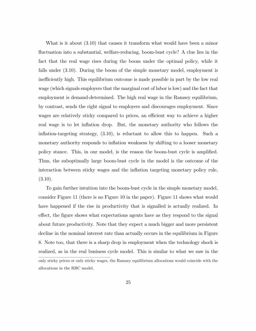
To gain further intuition into the boom-bust cycle in the simple monetary model,

consider Figure 11 (there is no Figure 10 in the paper). Figure 11 shows what would

have happened if the rise in productivity that is signalled is actually realized. In

effect, the figure shows what expectations agents have as they respond to the signal

about future productivity. Note that they expect a much bigger and more persistent

decline in the nominal interest rate than actually occurs in the equilibrium in Figure

8. Note too, that there is a sharp drop in employment when the technology shock is

realized, as in the real business cycle model. This is similar to what we saw in the

only sticky prices or only sticky wages, the Ramsey equilibrium allocations would coincide with the

allocations in the RBC model.

25

real business cycle analysis in Figure 3.

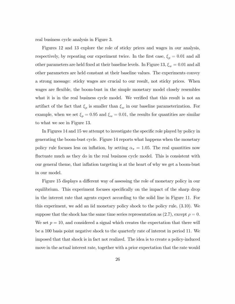
Figures 12 and 13 explore the role of sticky prices and wages in our analysis,

respectively, by repeating our experiment twice. In the first case, ξp = 0.01 and all

other parameters are held fixed at their baseline levels. In Figure 13, ξw = 0.01 and all

other parameters are held constant at their baseline values. The experiments convey

a strong message: sticky wages are crucial to our result, not sticky prices. When

wages are flexible, the boom-bust in the simple monetary model closely resembles

what it is in the real business cycle model. We verified that this result is not an

artifact of the fact that ξp is smaller than ξw in our baseline parameterization. For

example, when we set ξp = 0.95 and ξw = 0.01, the results for quantities are similar

to what we see in Figure 13.

In Figures 14 and 15 we attempt to investigate the specific role played by policy in

generating the boom-bust cycle. Figure 14 reports what happens when the monetary

policy rule focuses less on inflation, by setting απ = 1.05. The real quantities now

fluctuate much as they do in the real business cycle model. This is consistent with

our general theme, that inflation targeting is at the heart of why we get a boom-bust

in our model.

Figure 15 displays a different way of assessing the role of monetary policy in our

equilibrium. This experiment focuses specifically on the impact of the sharp drop

in the interest rate that agents expect according to the solid line in Figure 11. For

this experiment, we add an iid monetary policy shock to the policy rule, (3.10). We

suppose that the shock has the same time series representation as (2.7), except ρ = 0.

We set p = 10, and considered a signal which creates the expectation that there will

be a 100 basis point negative shock to the quarterly rate of interest in period 11. We

imposed that that shock is in fact not realized. The idea is to create a policy-induced

move in the actual interest rate, together with a prior expectation that the rate would

26

fall even more. Figure 15 indicates that this anticipated monetary loosening creates

a substantial boom right away in the model. The boom accounts for almost all of

the monetary part of the boom-bust in the simple monetary model. The vertical

difference between the two lines in Figure 15 is roughly the size of the boom in

the real business cycle model. The results in Figure 15 suggests the following loose

characterization of our boom-bust result in the simple monetary model: one-third

of the boom-bust cycle is the efficient response to a signal about technology, and

two-thirds of the boom-bust cycle is the inefficient consequence of suboptimality in

the monetary policy rule. This suboptimality operates by creating an expectation of

a substantial future anticipated loosening in monetary policy.

In sum, analysis with the simple monetary model suggests that successfully gener-

ating a substantial boom-bust episode requires a monetary policy rule which assigns

substantial weight to inflation and which incorporates sticky wages.

4. Full Monetary Model

We consider the full monetary model of Christiano, Motto and Rostagno(2006). That

model incorporates a banking sector following Chari, Christiano, and Eichenbaum

(1995) and the financial frictions in Bernanke, Gertler and Gilchrist (1999). In the

model, there are two financing requirements: (i) intermediate good firms require

funding in order to pay wages and capital rental costs and (ii) the capital is owned

and rented out by entrepreneurs, who do not have enough wealth (‘net worth’) on

their own to acquire the capital stock and so they must borrow. The working capital

lending in (i) is financed by demand deposits issued by banks to households. The

lending in (ii) is financed by savings deposits and time deposits issued to households.

Demand deposits and savings deposits pay interest, but relatively little, because they

27

generate utility services to households. Following Chari, Christiano, and Eichenbaum

(1995), the provision of demand and savings deposits by banks requires that they use

capital and labor resources, as well as reserves. Time deposits do not generate utility

services. In addition to holding demand, savings and time deposits, households also

hold currency because they generate utility services. Our measure of M1 in the model

is the sum of currency plus demand deposits. Our broader measure of money (we

could call it M2 or M3) is the sum of M1 and savings deposits. Total credit is the sum

of the lending done in (i) and (ii). Credit differs from money in that it includes time

deposits and does not include currency. Finally, the monetary base in the model is

the sum of currency plus bank reserves. A key feature of the model that allows it to

make contact with the literature on boom-busts is that it includes various monetary

aggregates as well as credit, and that their are nontrivial differences between these

aggregates.

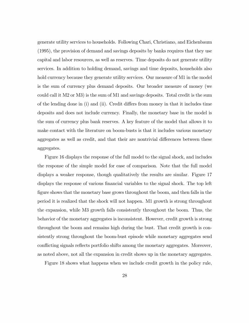
Figure 16 displays the response of the full model to the signal shock, and includes

the response of the simple model for ease of comparison. Note that the full model

displays a weaker response, though qualitatively the results are similar. Figure 17

displays the response of various financial variables to the signal shock. The top left

figure shows that the monetary base grows throughout the boom, and then falls in the

period it is realized that the shock will not happen. M1 growth is strong throughout

the expansion, while M3 growth falls consistently throughout the boom. Thus, the

behavior of the monetary aggregates is inconsistent. However, credit growth is strong

throughout the boom and remains high during the bust. That credit growth is con-

sistently strong throughout the boom-bust episode while monetary aggregates send

conflicting signals reflects portfolio shifts among the monetary aggregates. Moreover,

as noted above, not all the expansion in credit shows up in the monetary aggregates.

Figure 18 shows what happens when we include credit growth in the policy rule,

28

(3.10), with a coefficient of 3. The strong growth of credit leads to a tightening of

monetary policy during the boom, and causes the boom to more nearly resemble the

efficient response of the economy to the signal about future productivity.

In sum, we have simulated the response to a signal shock of a model with consid-

erably more frictions than those in our simple monetary model. The basic qualitative

findings of our simple model are robust to this added complexity.

5. Implications for Further Research

Sticky wages deserve to be taken seriously because they are a feature of models that

fit the data well. It is known that with sticky wages, a policy of targeting inflation can

lead to suboptimal results by making the real wage overly rigid. For example, if there

is a negative oil shock which requires that the real wage fall, a policy of preventing

the price level from rising will cause the real wage to be too high and employment

too low. In this paper we have shown that the type of boom-bust episodes we have

observed may be another example of the type of suboptimal outcome that can occur

in an economy with sticky wages and monetary targeting. Indeed, we argued that

within standard models it is hard to find another way to account for boom-bust

episodes.

We have not addressed the factors that make inflation targeting attractive. These

are principally the advantages that inflation targeting has for anchoring inflation

expectations. We are sympathetic to the view that these advantages argue in favor

of some sort of inflation-targeting in monetary policy. However, our results suggest

that it may be optimal to mitigate some of the negative consequences of inflation

targeting by also taking into account other variables. In particular, we have examined

the possibility that a policy which reacts to credit growth in addition to inflation may

29

reduce the likelihood that monetary policy inadvertently contributes to boom-bust

episodes.

Our argument remains tentative, even within the confines of the monetary economies

that we studied in this paper. We only showed that a monetary policy which feeds

back onto credit growth moves the response of the economy to a certain signal shock

closer to the optimal response. Such a policy would substantially reduce the vio-

lence of boom-bust episodes. However, a final assessment of the value of integrating

credit growth into monetary policy awaits an examination of how the response of

the economy to other shocks is affected. This work is currently under way. The

model of Christiano, Motto and Rostagno (2006) is ideally suited for this. Not only

does it contain a variety of credit measures, so that a serious consideration of the

consequences of integrating credit into monetary policy is possible. In addition, that

model is estimated with many shocks, making it possible to see how integrating credit

growth into monetary policy affects the transmission of shocks.

30

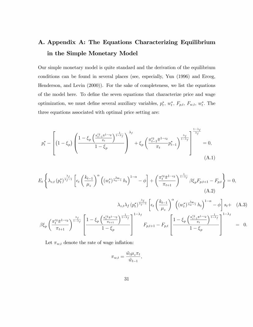
A. Appendix A: The Equations Characterizing Equilibrium

in the Simple Monetary Model

Our simple monetary model is quite standard and the derivation of the equilibrium

conditions can be found in several places (see, especially, Yun (1996) and Erceg,

Henderson, and Levin (2000)). For the sake of completeness, we list the equations

of the model here. To define the seven equations that characterize price and wage

optimization, we must define several auxiliary variables, p∗t , w∗t , Fp,t, Fw,t, w

∗t . The

three equations associated with optimal price setting are:

p∗t −

⎡⎢⎢⎣¡1− ξp¢⎛⎜⎝1− ξp

³πι2t−1π̄

1−ι2

πt

´ 11−λf

1− ξp

⎞⎟⎠λf

+ ξp

µπι2t−1π̄

1−ι2

πtp∗t−1

¶ λf1−λf

⎤⎥⎥⎦1−λfλf

= 0,

(A.1)

Et

(λz,t (p

∗t )

λfλf−1

∙t

µkt−1µz

¶α ³(w∗t )

λwλw−1 ht

´1−α− φ

¸+

µπι2t π̄

1−ι2

πt+1

¶ 11−λf

βξpFp,t+1 − Fp,t

)= 0,

(A.2)

λz,tλf (p∗t )

λfλf−1

∙t

µkt−1µz

¶α ³(w∗t )

λwλw−1 ht

´1−α− φ

¸st+ (A.3)

βξp

µπι2t π̄

1−ι2

πt+1

¶ λf1−λf

⎡⎢⎣1− ξp

³πι2t π̄1−ι2

πt+1

´ 11−λf

1− ξp

⎤⎥⎦1−λf

Fp,t+1 − Fp,t

⎡⎢⎣1− ξp

³πι2t−1π̄

1−ι2

πt

´ 11−λf

1− ξp

⎤⎥⎦1−λf

= 0.

Let πw,t denote the rate of wage inflation:

πw,t =w̃tµzπtw̃t−1

,

31

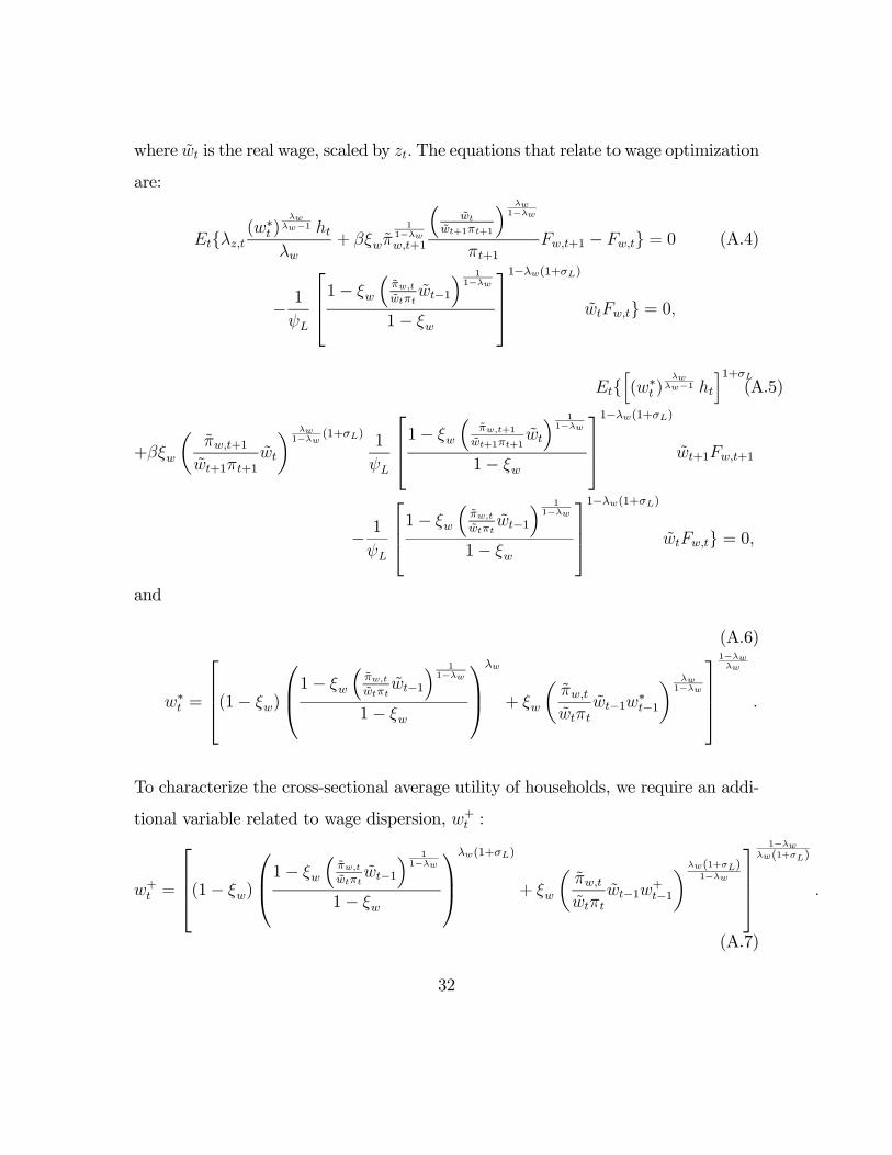
where w̃t is the real wage, scaled by zt. The equations that relate to wage optimization

are:

Et{λz,t(w∗t )

λwλw−1 htλw

+ βξwπ̃1

1−λww,t+1

³w̃t

w̃t+1πt+1

´ λw1−λw

πt+1Fw,t+1 − Fw,t} = 0 (A.4)

− 1

ψL

⎡⎢⎣1− ξw

³π̃w,tw̃tπt

w̃t−1

´ 11−λw

1− ξw

⎤⎥⎦1−λw(1+σL)

w̃tFw,t} = 0,

Et{h(w∗t )

λwλw−1 ht

i1+σL(A.5)

+βξw

µπ̃w,t+1

w̃t+1πt+1w̃t

¶ λw1−λw (1+σL) 1

ψL

⎡⎢⎣1− ξw

³π̃w,t+1

w̃t+1πt+1w̃t

´ 11−λw

1− ξw

⎤⎥⎦1−λw(1+σL)

w̃t+1Fw,t+1

− 1

ψL

⎡⎢⎣1− ξw

³π̃w,tw̃tπt

w̃t−1

´ 11−λw

1− ξw

⎤⎥⎦1−λw(1+σL)

w̃tFw,t} = 0,

and

(A.6)

w∗t =

⎡⎢⎢⎣(1− ξw)

⎛⎜⎝1− ξw

³π̃w,tw̃tπt

w̃t−1

´ 11−λw

1− ξw

⎞⎟⎠λw

+ ξw

µπ̃w,tw̃tπt

w̃t−1w∗t−1

¶ λw1−λw

⎤⎥⎥⎦1−λwλw

.

To characterize the cross-sectional average utility of households, we require an addi-

tional variable related to wage dispersion, w+t :

w+t =

⎡⎢⎢⎣(1− ξw)

⎛⎜⎝1− ξw

³π̃w,tw̃tπt

w̃t−1

´ 11−λw

1− ξw

⎞⎟⎠λw(1+σL)

+ ξw

µπ̃w,tw̃tπt

w̃t−1w+t−1

¶λw(1+σL)1−λw

⎤⎥⎥⎦1−λw

λw(1+σL)

.

(A.7)

32

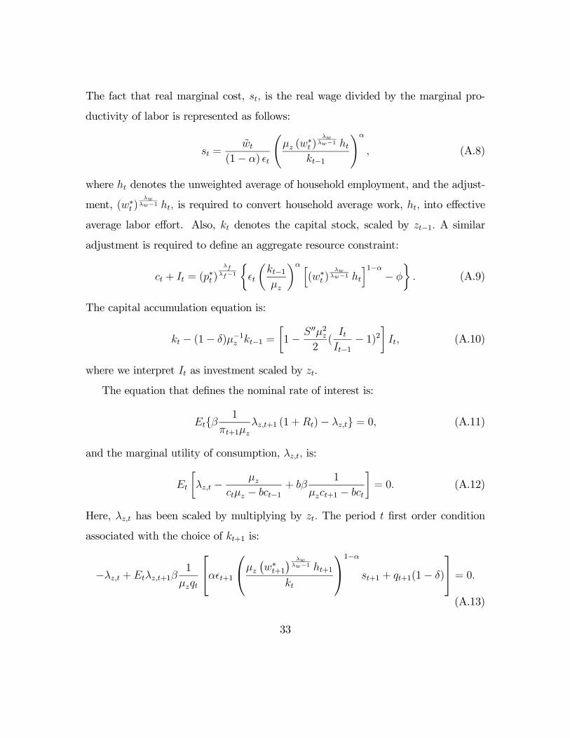
The fact that real marginal cost, st, is the real wage divided by the marginal pro-

ductivity of labor is represented as follows:

st =w̃t

(1− α) t

Ãµz (w

∗t )

λwλw−1 ht

kt−1

!α

, (A.8)

where ht denotes the unweighted average of household employment, and the adjust-

ment, (w∗t )λw

λw−1 ht, is required to convert household average work, ht, into effective

average labor effort. Also, kt denotes the capital stock, scaled by zt−1. A similar

adjustment is required to define an aggregate resource constraint:

ct + It = (p∗t )

λfλf−1

½t

µkt−1µz

¶α h(w∗t )

λwλw−1 ht

i1−α− φ

¾. (A.9)

The capital accumulation equation is:

kt − (1− δ)µ−1z kt−1 =

∙1− S00µ2z

2(ItIt−1− 1)2

¸It, (A.10)

where we interpret It as investment scaled by zt.

The equation that defines the nominal rate of interest is:

Et{β1

πt+1µzλz,t+1 (1 +Rt)− λz,t} = 0, (A.11)

and the marginal utility of consumption, λz,t, is:

Et

∙λz,t −

µzctµz − bct−1

+ bβ1

µzct+1 − bct

¸= 0. (A.12)

Here, λz,t has been scaled by multiplying by zt. The period t first order condition

associated with the choice of kt+1 is:

−λz,t +Etλz,t+1β1

µzqt

⎡⎣α t+1

⎛⎝µz¡w∗t+1

¢ λwλw−1 ht+1

kt

⎞⎠1−α

st+1 + qt+1(1− δ)

⎤⎦ = 0.(A.13)

33

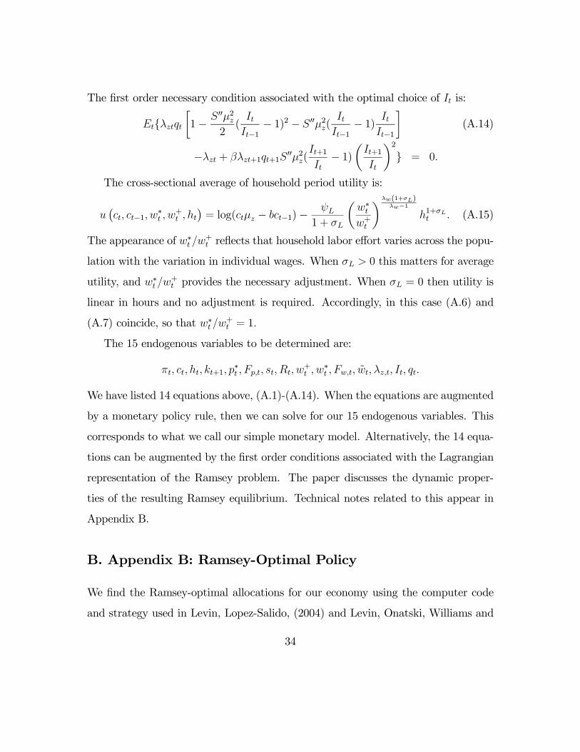
The first order necessary condition associated with the optimal choice of It is:

Et{λztqt∙1− S00µ2z

2(ItIt−1− 1)2 − S00µ2z(

ItIt−1− 1) It

It−1

¸(A.14)

−λzt + βλzt+1qt+1S00µ2z(

It+1It− 1)

µIt+1It

¶2} = 0.

The cross-sectional average of household period utility is:

u¡ct, ct−1, w

∗t , w

+t , ht

¢= log(ctµz − bct−1)−

ψL

1 + σL

µw∗tw+t

¶λw(1+σL)λw−1

h1+σLt . (A.15)

The appearance of w∗t /w+t reflects that household labor effort varies across the popu-

lation with the variation in individual wages. When σL > 0 this matters for average

utility, and w∗t /w+t provides the necessary adjustment. When σL = 0 then utility is

linear in hours and no adjustment is required. Accordingly, in this case (A.6) and

(A.7) coincide, so that w∗t /w+t = 1.

The 15 endogenous variables to be determined are:

πt, ct, ht, kt+1, p∗t , Fp,t, st, Rt, w

+t , w

∗t , Fw,t, w̃t, λz,t, It, qt.

We have listed 14 equations above, (A.1)-(A.14). When the equations are augmented

by a monetary policy rule, then we can solve for our 15 endogenous variables. This

corresponds to what we call our simple monetary model. Alternatively, the 14 equa-

tions can be augmented by the first order conditions associated with the Lagrangian

representation of the Ramsey problem. The paper discusses the dynamic proper-

ties of the resulting Ramsey equilibrium. Technical notes related to this appear in

Appendix B.

B. Appendix B: Ramsey-Optimal Policy

We find the Ramsey-optimal allocations for our economy using the computer code

and strategy used in Levin, Lopez-Salido, (2004) and Levin, Onatski, Williams and

34

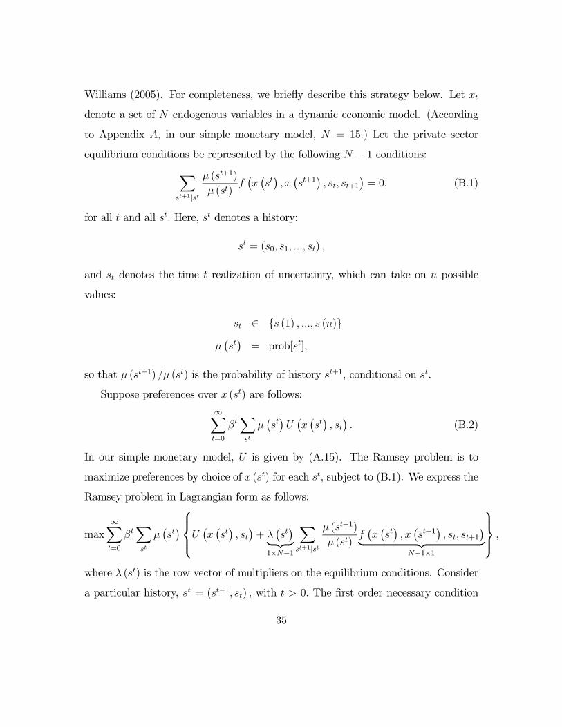
Williams (2005). For completeness, we briefly describe this strategy below. Let xt

denote a set of N endogenous variables in a dynamic economic model. (According

to Appendix A, in our simple monetary model, N = 15.) Let the private sector

equilibrium conditions be represented by the following N − 1 conditions:Xst+1|st

µ (st+1)

µ (st)f¡x¡st¢, x¡st+1

¢, st, st+1

¢= 0, (B.1)

for all t and all st. Here, st denotes a history:

st = (s0, s1, ..., st) ,

and st denotes the time t realization of uncertainty, which can take on n possible

values:

st ∈ {s (1) , ..., s (n)}

µ¡st¢= prob[st],

so that µ (st+1) /µ (st) is the probability of history st+1, conditional on st.

Suppose preferences over x (st) are follows:

∞Xt=0

βtXst

µ¡st¢U¡x¡st¢, st¢. (B.2)

In our simple monetary model, U is given by (A.15). The Ramsey problem is to

maximize preferences by choice of x (st) for each st, subject to (B.1). We express the

Ramsey problem in Lagrangian form as follows:

max∞Xt=0

βtXst

µ¡st¢⎧⎪⎨⎪⎩U

¡x¡st¢, st¢+ λ

¡st¢| {z }

1×N−1

Xst+1|st

µ (st+1)

µ (st)f¡x¡st¢, x¡st+1

¢, st, st+1

¢| {z }N−1×1

⎫⎪⎬⎪⎭ ,

where λ (st) is the row vector of multipliers on the equilibrium conditions. Consider

a particular history, st = (st−1, st) , with t > 0. The first order necessary condition

35

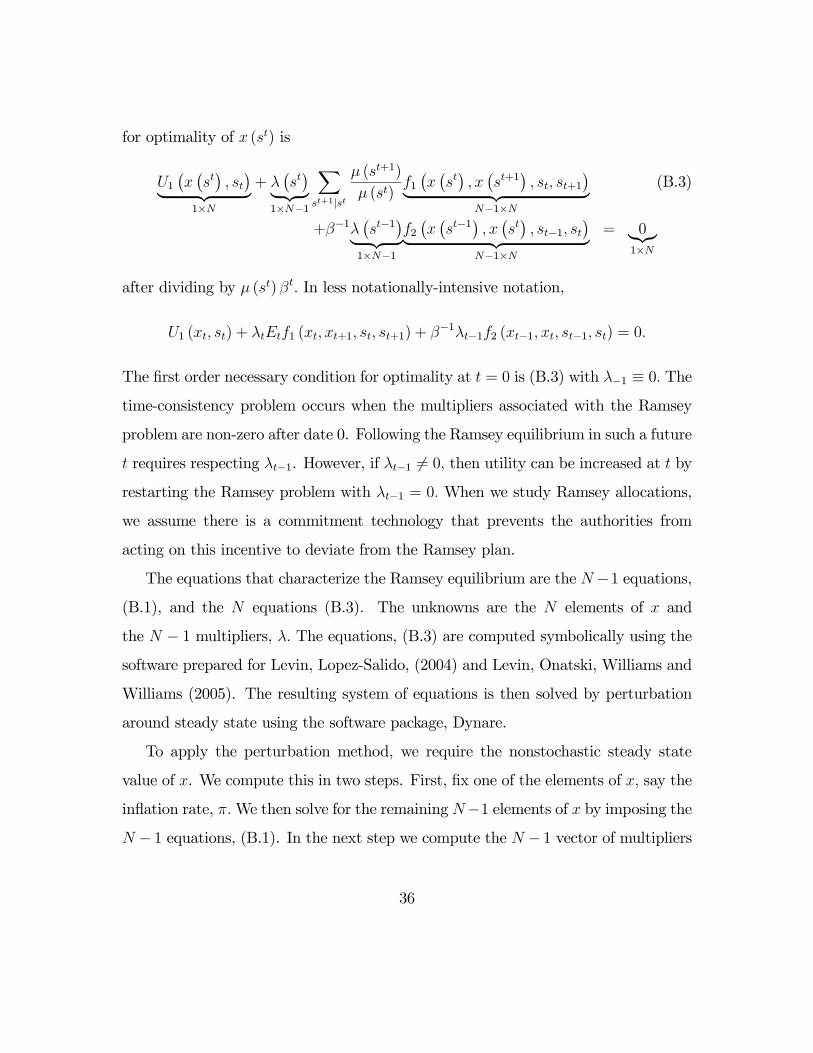
for optimality of x (st) is

U1¡x¡st¢, st¢| {z }

1×N

+ λ¡st¢| {z }

1×N−1

Xst+1|st

µ (st+1)

µ (st)f1¡x¡st¢, x¡st+1

¢, st, st+1

¢| {z }N−1×N

(B.3)

+β−1λ¡st−1

¢| {z }1×N−1

f2¡x¡st−1

¢, x¡st¢, st−1, st

¢| {z }N−1×N

= 0|{z}1×N

after dividing by µ (st)βt. In less notationally-intensive notation,

U1 (xt, st) + λtEtf1 (xt, xt+1, st, st+1) + β−1λt−1f2 (xt−1, xt, st−1, st) = 0.

The first order necessary condition for optimality at t = 0 is (B.3) with λ−1 ≡ 0. The

time-consistency problem occurs when the multipliers associated with the Ramsey

problem are non-zero after date 0. Following the Ramsey equilibrium in such a future

t requires respecting λt−1. However, if λt−1 6= 0, then utility can be increased at t by

restarting the Ramsey problem with λt−1 = 0. When we study Ramsey allocations,

we assume there is a commitment technology that prevents the authorities from

acting on this incentive to deviate from the Ramsey plan.

The equations that characterize the Ramsey equilibrium are the N−1 equations,

(B.1), and the N equations (B.3). The unknowns are the N elements of x and

the N − 1 multipliers, λ. The equations, (B.3) are computed symbolically using the

software prepared for Levin, Lopez-Salido, (2004) and Levin, Onatski, Williams and

Williams (2005). The resulting system of equations is then solved by perturbation

around steady state using the software package, Dynare.

To apply the perturbation method, we require the nonstochastic steady state

value of x. We compute this in two steps. First, fix one of the elements of x, say the

inflation rate, π.We then solve for the remaining N−1 elements of x by imposing the

N − 1 equations, (B.1). In the next step we compute the N − 1 vector of multipliers

36

using the steady state version of (B.3):

U1 + λ£f1 + β−1f2

¤= 0,

where a function without an explicit argument is understood to mean it is evaluated

in steady state.5 Write

Y = U 01

X =£f1 + β−1f2

¤0β = λ0,

so that Y is an N × 1 column vector, X is an N × (N − 1) matrix and β is an

(N − 1)× 1 column vector. Compute β and u as

β = (X 0X)−1

X 0Y

u = Y −Xβ.

Note that this regression will not in general fit perfectly, because there are N − 1

‘explanatory variables’ and N elements of Y to ‘explain’. We vary the value of π

until max |ui| = 0. This completes the discussion of the calculation of the steady

state and of the algorithm for computing Ramsey allocations.

5This step is potentially very cumbersome, but has been made relatively easy by the software

produced for Levin, Lopez-Salido, (2004) and Levin, Onatski, Williams and Williams (2005). This

sofware endogenously writes the code necessary to solve for the multipliers.

37

References

[1] Adalid, Ramon, and Carsten Detken, 2006, ‘Excessive Liquidity and Asset Price

Boom/Bust Cycles,’ manuscript, European Central Bank.

[2] Barro, Robert, and Robert King, 1984, ‘Time Separable Preferences and In-

tertemporal Substitution Models of Business Cycles,’ Quarterly Journal of Eco-

nomics, 99 (4), pp. 817-39.

[3] Beaudry, Paul and Franck Portier, 2000, ‘An Exploration into Pigou’s Theory

of Cycles,’ Journal of Monetary Economics, University of British Columbia.

[4] Beaudry, Paul and Franck Portier, 2003, ‘Expectationally Driven Booms and

Busts in Equilibrium Cycle Models,’ mimeo, University of British Columbia.

[5] Beaudry, Paul and Franck Portier, 2004, ‘Stock Prices, News and Economic

Fluctuations,’ manuscript.

[6] Bernanke, Ben, and Mark Gertler, 2000, ‘Monetary Policy and Asset Price

Volatility,’ NBER working paper number 7559.

[7] Bernanke, Ben, Mark Gertler and Simon Gilchrist. (1999). “The Financial Ac-

celerator in a Quantitative Business Cycle Framework.” Handbook of Macro-

economics, edited by John B. Taylor and Michael Woodford, pp. 1341-93. Am-

sterdam, New York and Oxford: Elsevier Science, North-Holland.

[8] Blanchard, Olivier, and Jordi Galí, 2006, ‘A New Keynesian Model with Unem-

ployment,’ manuscript.

38

[9] Chari, V.V., Lawrence J. Christiano, and Martin Eichenbaum, 1995, “Inside

Money, Outside Money and Short Term Interest Rates.” Journal of Money,

Credit and Banking 27, 1354-86.

[10] Christiano, Eichenbaum and Evans, 2004, ‘Nominal Rigidities and the Dynamic

Effects of a Shock to Monetary Policy’, Journal of Political Economy.

[11] Eichengreen, Barry, and Kris Mitchener, 2003, ‘The Great Depression as a

Credit Boom Gone Wrong,’ Bank for International Settlements working paper

no. 137.

[12] Erceg, Christopher, Dale Henderson, and Andrew Levin, 2000, ‘Optimal Mon-

etary Policy with Staggered Wage and Price Contracts,’ Journal of Monetary

Economics, 46, 281-313.

[13] Gali, Jordi, Mark Gertler and David Lopes-Salido, forthcoming, ‘Markups, Gaps

and the Welfare Costs of Business Cycles,’ Review of Economics and Statistics.

[14] Jaimovich, Nir, and Sergio Rebelo, 2006, ‘Do News Shocks Drive the Business

Cycle?,’ Northwestern University.

[15] Yun, Tack, 1996, ‘Nominal Price Rigidity, Money Supply Endogeneity, and Busi-

ness Cycles,’ Journal of Monetary Economics, 37(2): 345 - 370.

39

1880 1900 1920 1940 1960 1980 2000

200

400

600

800

1000

1200

1400

1600

Figure 1: S&P500 Divided by CPI (Shiller)

1924 1926 1928 1930 1932-2

-1.5

-1

-0.5

0

0.5

1

1.5

2

2.5

Fig 2A: Standardized inflation and stock price in interwar period

1955 1960 1965 1970 1975

-1

0

1

2

3

Fig 2B: Standardized inflation and stock price in 1950's to 1970's period

1980 1985 1990 1995 2000 2005

-1

0

1

2

3

4Fig 2C: Standardized inflation and stock price in interwar period

Inflation

S&P500

2 4 6 8

0.1

0.2

0.3

0.4

0.5

0.6

0.7

t

perc

ent

Output

2 4 6 8

0.2

0.3

0.4

0.5

0.6

0.7

0.8

0.9

tperc

ent

Investment

2 4 6 8

0

0.1

0.2

0.3

0.4

0.5

0.6

t

perc

ent

Consumption

2 4 6 8-0.6

-0.4

-0.2

0

0.2

0.4

t

perc

ent

Hours Worked

2 4 6 8

-200

0

200

400

600

800

1000

t

basis

poin

ts

Riskfree rate with payoff in t+1 (annual)

Figure 3: Real Business Cycle Model with Habit and CEE Investment Adjustment Costs Baseline - Tech Shock Not Realized, Perturbation - Tech Shock Realized in Period 5

2 4 6 8

-0.5

0

0.5

1

1.5

t

perc

ent

Pk'

Perturbed RBC Model

Baseline RBC Model

2 4 6 8

0.05

0.1

0.15

0.2

0.25

0.3

t

perc

ent

Output

2 4 6 8

0.15

0.2

0.25

0.3

0.35

0.4

0.45

0.5

tperc

ent

Investment

2 4 6 8

-0.15

-0.1

-0.05

0

0.05

0.1

0.15

0.2

t

perc

ent

Consumption

2 4 6 8

0.05

0.1

0.15

0.2

0.25

0.3

0.35

0.4

0.45

0.5

t

perc

ent

Hours Worked

2 4 6 8

0

200

400

600

800

1000

t

basis

poin

ts


Figure 4: Real Business Cycle Model without Habit and with CEE Investment Adjustment Costs Technology Shock Not Realized in Period 5

2 4 6 8

-0.8

-0.7

-0.6

-0.5

-0.4

-0.3

-0.2

t

perc

ent

Pk'

Perturbed RBC Model

Baseline RBC Model

2 4 6 8-0.1

-0.05

0

0.05

0.1

0.15

0.2

0.25

0.3

t

perc

ent

Output

2 4 6 8-0.4

-0.3

-0.2

-0.1

0

0.1

0.2

0.3

0.4

0.5

tperc

ent

Investment

2 4 6 8-0.05

0

0.05

0.1

0.15

0.2

t

perc

ent

Consumption

2 4 6 8-0.1

0

0.1

0.2

0.3

0.4

0.5

t

perc

ent

Hours Worked

2 4 6 8

0

200

400

600

800

1000

t

basis

poin

ts


Figure 5: Real Business Cycle Model with Habit and Without Investment Adjustment Costs Technology Shock not Realized in Period 5

2 4 6 8

-0.8

-0.6

-0.4

-0.2

0

0.2

t

perc

ent

Pk'

Perturbed RBC Model

Baseline RBC Model

2 4 6 8

0.05

0.1

0.15

0.2

0.25

0.3

t

perc

ent

Output

2 4 6 8

-0.2

-0.1

0

0.1

0.2

0.3

0.4

0.5

tperc

ent

Investment

2 4 6 8

0

0.05

0.1

0.15

0.2

0.25

t

perc

ent

Consumption

2 4 6 8

0.05

0.1

0.15

0.2

0.25

0.3

0.35

0.4

0.45

0.5

t

perc

ent

Hours Worked

2 4 6 8

0

200

400

600

800

1000

t

basis

poin

ts


Figure 6: Real Business Cycle Model with Habit and with Level Investment Adjustment Costs Technology Shock Not Realized in Period 5

2 4 6 8

-0.8

-0.7

-0.6

-0.5

-0.4

-0.3

-0.2

-0.1

t

perc

ent

Pk'

Perturbed RBC Model

Baseline RBC Model

5 10 15 200

0.05

0.1

0.15

0.2

0.25

0.3

0.35

t

perc

ent

Output

Perturbed RBC Model

Baseline RBC Model

5 10 15 20

0.1

0.2

0.3

0.4

0.5

0.6

t

perc

ent

Investment

5 10 15 20-0.05

0

0.05

0.1

0.15

0.2

t

perc

ent

Consumption

5 10 15 200

0.1

0.2

0.3

0.4

0.5

t

perc

ent

Hours Worked

5 10 15 20

0

200

400

600

800

1000


t

basis

poin

ts

Figure 7: Real Business Cycle Model with Habit Persistence and Flow Adjustment Costs Perturbed - Technology Shock Expected in Period 13, But Not Realized

5 10 15 20

-0.9

-0.8

-0.7

-0.6

-0.5

-0.4

-0.3

-0.2

-0.1

t

perc

ent

Pk'

5 10 15 200

0.2

0.4

0.6

0.8

1

perc

ent

Output

5 10 15 20

0.5

1

1.5

perc

ent

Investment

Simple Monetary Model

Real Business Cycle Model

5 10 15 20

0

0.2

0.4

0.6

perc

ent

Consumption

5 10 15 200

0.5

1

perc

ent

Hours Worked

5 10 15 20

-0.8

-0.6

-0.4

-0.2

0

0.2

Inflation (APR)

5 10 15 20

0

500

1000

Ex post realized real Rt+1

e/

t+1 (annual)

basis

poin

ts

5 10 15 20

-0.3

-0.2

-0.1

0

real wage

perc

ent

5 10 15 20-80

-60

-40

-20

0

20

Nominal rate of interest (Rt+1

e, annual)

basis

poin

ts

Figure 8: RBC and Simple Monetary ModelExpectation of Technology Shock in Period 13 Not Realized

5 10 15 20

-0.8

-0.6

-0.4

-0.2

0

0.2

perc

ent

Pk'

Note: subscript on nominal rate of interest indicates date of payoff. Rt+1

e is graphed at date t.

t indicates gross change in price level from t-1 to t.

5 10 15 200

0.2

0.4

0.6

0.8

1

outputperc

ent devia

tion fro

m s

s

5 10 15 20

0

0.2

0.4

0.6

consumption

perc

ent devia

tion fro

m s

s

Ramsey Equilibrium of Simple Monetary ModelSimple Monetary Model

5 10 15 20

2

4

6

8

10

12

14

net real rate of interest

annualiz

ed, perc

ent

5 10 15 200

0.5

1

hours worked

perc

ent devia

tion fro

m s

s

5 10 15 20

1.6

1.8

2

2.2

2.4

net inflation (APR)

5 10 15 200

0.5

1

1.5

investment

perc

ent devia

tion fro

m s

s

5 10 15 20

4

6

8

10

12

14

Annualiz

ed, perc

ent

net nominal rate of interest

5 10 15 20

-1

-0.5

0

perc

ent devia

tion fro

m s

s

price of capital

Figure 9: Simple Monetary Model and Associated Ramsey Equilibrium

5 10 15 20

-0.2

-0.1

0

0.1

0.2

perc

ent devia

tion fro

m s

s

real wage

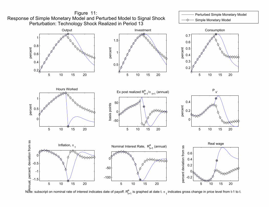
5 10 15 20

0.2

0.4

0.6

0.8

1

perc

ent

Output

Perturbed Simple Monetary Model


5 10 15 20

0.5

1

1.5

Investment

perc

ent

5 10 15 20

0.2

0.3

0.4

0.5

0.6

0.7

Consumption

perc

ent

5 10 15 20

0

0.5

1

Hours Worked

perc

ent

5 10 15 20

-50

0

50

basis

poin

ts

Ex post realized Re

t+1/

t+1 (annual)

5 10 15 20

0

0.2

0.4

Pk'

perc

ent

5 10 15 20

-1.5

-1

-0.5

0

Inflation,t

Annual, p

erc

ent, d

evia

tion fro

m s

s

5 10 15 20

-100

-50

0

Nominal Interest Rate, Rt+1

e (annual)

Figure 11: Response of Simple Monetary Model and Perturbed Model to Signal Shock

Perturbation: Technology Shock Realized in Period 13

5 10 15 20

-0.2

0

0.2

0.4

0.6

Real wage

perc

ent devia

tion fro

m s

s




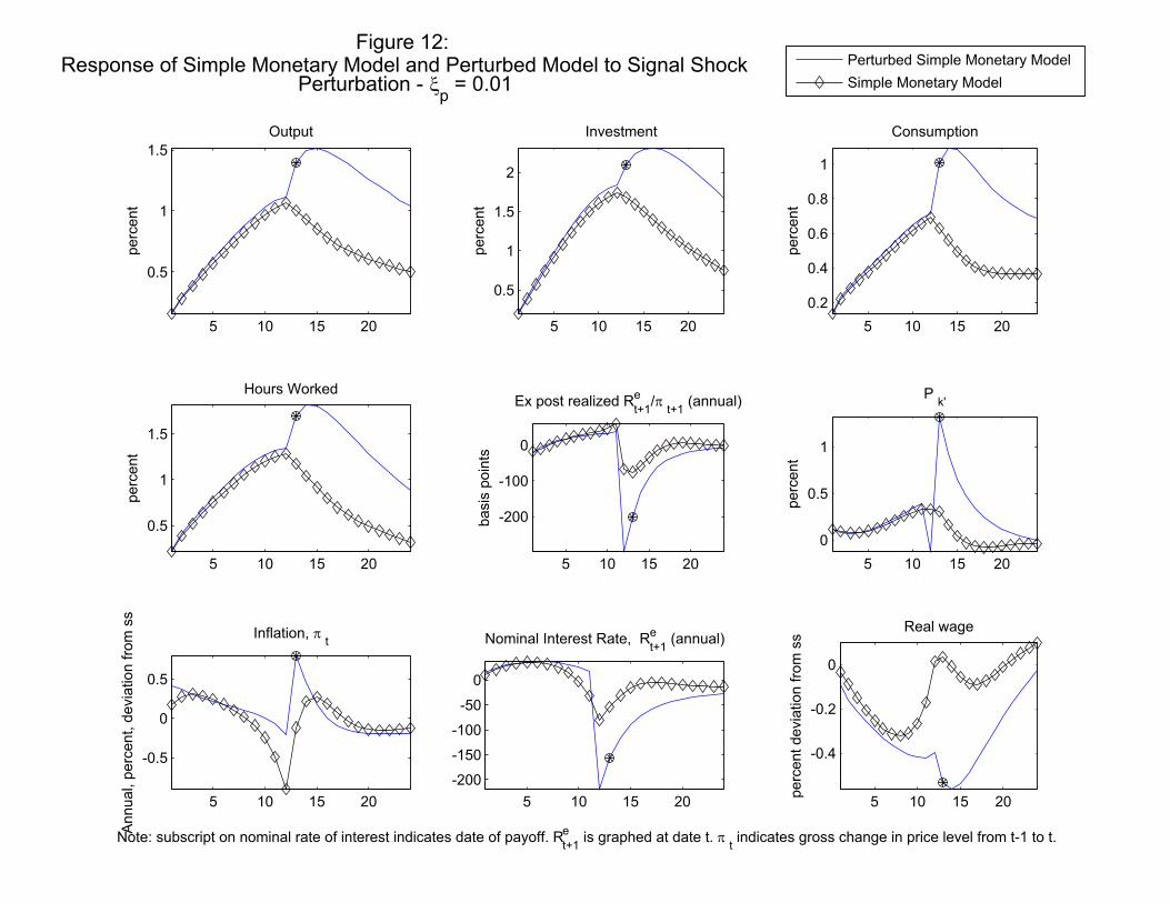
5 10 15 20

0.5

1

1.5

perc

ent

Output



5 10 15 20

0.5

1

1.5

2

Investment

perc

ent

5 10 15 20

0.2

0.4

0.6

0.8

1

Consumption

perc

ent

5 10 15 20

0.5

1

1.5

Hours Worked

perc

ent

5 10 15 20

-200

-100

0

basis

poin

ts

Ex post realized Re

t+1/

t+1 (annual)

5 10 15 20

0

0.5

1

Pk'

perc

ent

5 10 15 20

-0.5

0

0.5

Inflation,t

Annual, p

erc

ent, d

evia

tion fro

m s

s

5 10 15 20

-200

-150

-100

-50

0


e (annual)


Perturbation - p = 0.01

5 10 15 20

-0.4

-0.2

0

Real wage

perc

ent devia

tion fro

m s

s




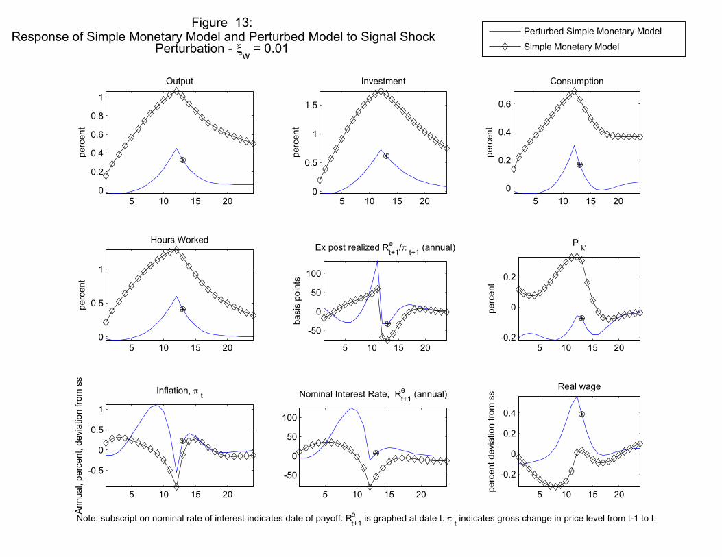
5 10 15 20

0

0.2

0.4

0.6

0.8

1

perc

ent

Output



5 10 15 200

0.5

1

1.5

Investment

perc

ent

5 10 15 20

0

0.2

0.4

0.6

Consumption

perc

ent

5 10 15 20

0

0.5

1

Hours Worked

perc

ent

5 10 15 20

-50

0

50

100

basis

poin

ts

Ex post realized Re

t+1/

t+1 (annual)

5 10 15 20-0.2

0

0.2

Pk'

perc

ent

5 10 15 20

-0.5

0

0.5

1

Inflation,t

Annual, p

erc

ent, d

evia

tion fro

m s

s

5 10 15 20

-50

0

50

100


e (annual)


Perturbation - w

= 0.01

5 10 15 20

-0.2

0

0.2

0.4

Real wage

perc

ent devia

tion fro

m s

s




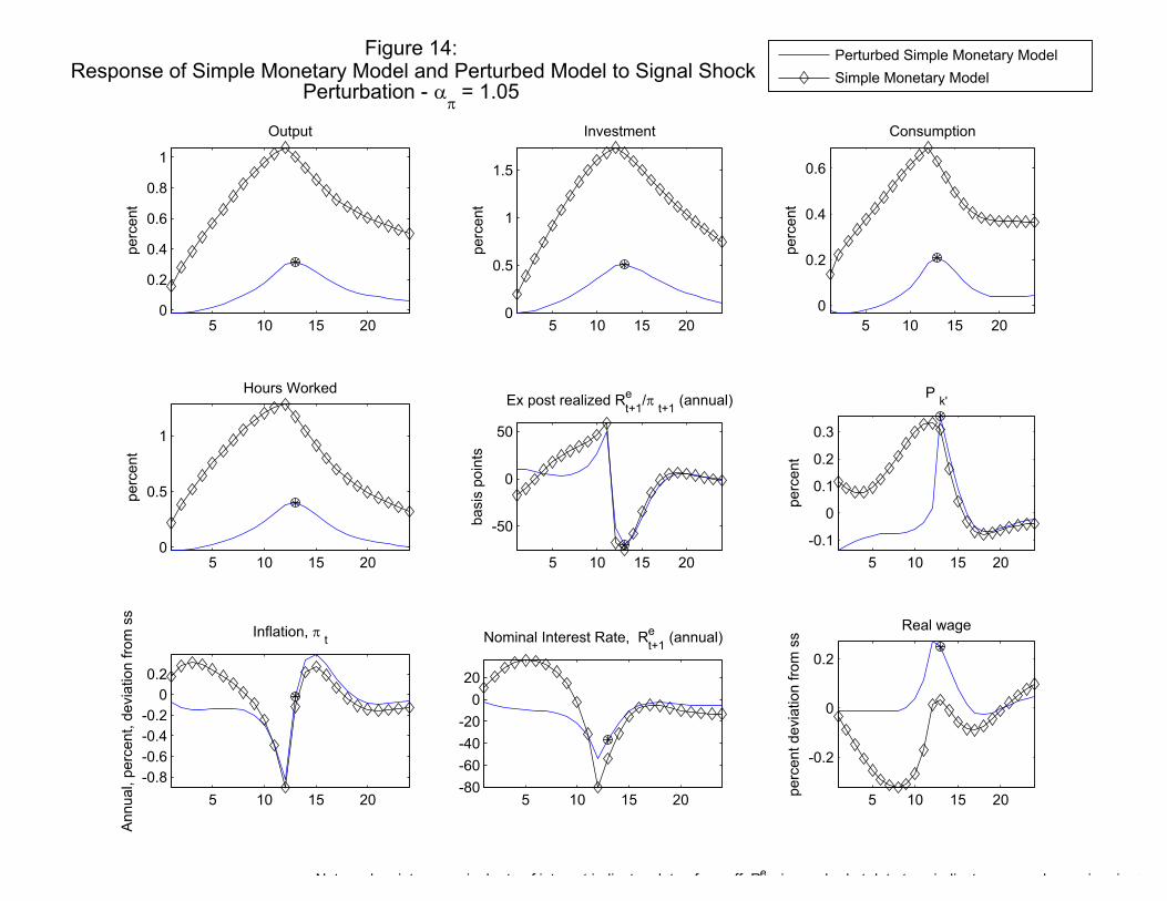
5 10 15 200

0.2

0.4

0.6

0.8

1

perc

ent

Output



5 10 15 200

0.5

1

1.5

Investment

perc

ent

5 10 15 20

0

0.2

0.4

0.6

Consumption

perc

ent

5 10 15 200

0.5

1

Hours Worked

perc

ent

5 10 15 20

-50

0

50

basis

poin

ts

Ex post realized Re

t+1/

t+1 (annual)

5 10 15 20

-0.1

0

0.1

0.2

0.3

Pk'

perc

ent

5 10 15 20

-0.8

-0.6

-0.4

-0.2

0

0.2

Inflation,t

Annual, p

erc

ent, d

evia

tion fro

m s

s

5 10 15 20-80

-60

-40

-20

0

20


e (annual)


Perturbation - = 1.05

5 10 15 20

-0.2

0

0.2

Real wage

perc

ent devia

tion fro

m s

s

N t b i t i l t f i t t i di t d t f ff Re

i h d t d t t i di t h i i l

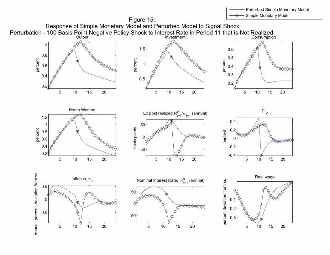
5 10 15 20

0.2

0.4

0.6

0.8

1

perc

ent

Output



5 10 15 20

0.5

1

1.5

Investment

perc

ent

5 10 15 20

0.2

0.3

0.4

0.5

0.6

Consumption

perc

ent

5 10 15 20

0.2

0.4

0.6

0.8

1

1.2

Hours Worked

perc

ent

5 10 15 20

-50

0

50

basis

poin

ts

Ex post realized Re

t+1/

t+1 (annual)

5 10 15 20-0.4

-0.2

0

0.2

0.4

Pk'

perc

ent

5 10 15 20

-0.5

0

0.5

Inflation,t

Annual, p

erc

ent, d

evia

tion fro

m s

s

5 10 15 20

-50

0

50


e (annual)


Perturbation - 100 Basis Point Negative Policy Shock to Interest Rate in Period 11 that is Not Realized

5 10 15 20

-0.3

-0.2

-0.1

0

Real wage

perc

ent devia

tion fro

m s

s

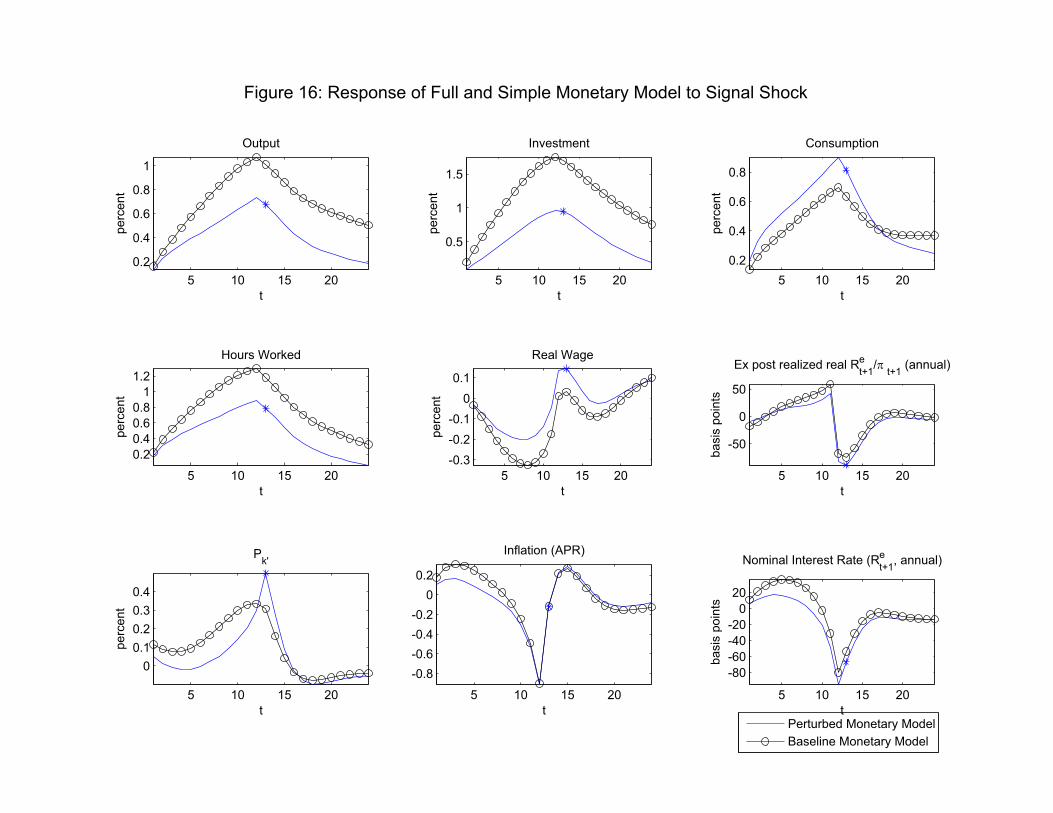
5 10 15 20

0.2

0.4

0.6

0.8

1

t

perc

ent

Output

Perturbed Monetary Model

Baseline Monetary Model

5 10 15 20

0.5

1

1.5

t

perc

ent

Investment

5 10 15 20

0.2

0.4

0.6

0.8

t

perc

ent

Consumption

5 10 15 20

0.2

0.4

0.6

0.8

1

1.2

t

perc

ent

Hours Worked

5 10 15 20

-0.3

-0.2

-0.1

0

0.1

t

perc

ent

Real Wage

5 10 15 20

-50

0

50


e/

t+1 (annual)

t

basis

poin

ts

5 10 15 20

0

0.1

0.2

0.3

0.4

perc

ent

t

Pk'

5 10 15 20

-0.8

-0.6

-0.4

-0.2

0

0.2

t

Inflation (APR)

Figure 16: Response of Full and Simple Monetary Model to Signal Shock

5 10 15 20

-80

-60

-40

-20

0

20

basis

poin

tst

Nominal Interest Rate (Rt+1

e, annual)

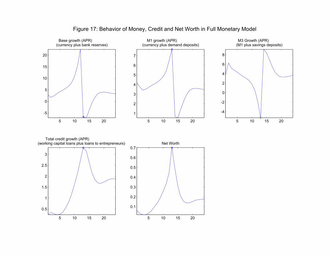
5 10 15 20

-5

0

5

10

15

20

Base growth (APR)(currency plus bank reserves)

5 10 15 20

1

2

3

4

5

6

7

M1 growth (APR)(currency plus demand deposits)

5 10 15 20

-4

-2

0

2

4

6

8

M3 Growth (APR)(M1 plus savings deposits)

5 10 15 20

0.5

1

1.5

2

2.5

3

Total credit growth (APR)(working capital loans plus loans to entrepreneurs)

Figure 17: Behavior of Money, Credit and Net Worth in Full Monetary Model

5 10 15 20

0.1

0.2

0.3

0.4

0.5

0.6

0.7Net Worth

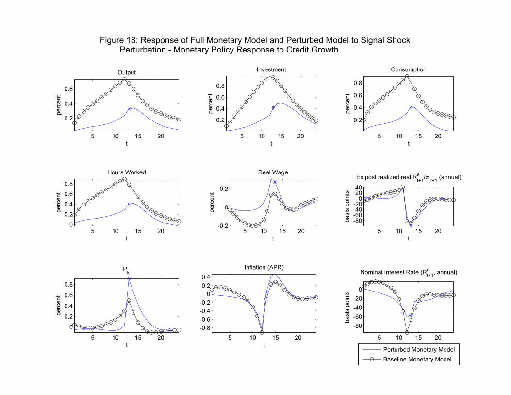
5 10 15 20

0.2

0.4

0.6

t

perc

ent

Output

5 10 15 20

0.2

0.4

0.6

0.8

t

perc

ent

Investment

5 10 15 20

0.2

0.4

0.6

0.8

t

perc

ent

Consumption

5 10 15 200

0.2

0.4

0.6

0.8

t

perc

ent

Hours Worked

5 10 15 20-0.2

0

0.2

t

perc

ent

Real Wage

5 10 15 20

-80-60-40-20

02040


e/

t+1 (annual)

t

basis

poin

ts

5 10 15 20

0

0.2

0.4

0.6

0.8

perc

ent

t

Pk'

5 10 15 20

-0.8

-0.6

-0.4

-0.2

0

0.2

0.4

t

Inflation (APR)

Figure 18: Response of Full Monetary Model and Perturbed Model to Signal ShockPerturbation - Monetary Policy Response to Credit Growth

5 10 15 20

-80

-60

-40

-20

0

basis

poin

tst

Nominal Interest Rate (Rt+1

e, annual)

Perturbed Monetary Model

Baseline Monetary Model

monetary policy and stock market boom-bust cycles policy and stock market boom-bust cycles∗...

Documents