FEDERAL RESERVE BANK OF SAN FRANCISCO

WORKING PAPER SERIES

Working Paper 2009-16 http://www.frbsf.org/publications/economics/papers/2009/wp09-16bk.pdf

The views in this paper are solely the responsibility of the authors and should not be interpreted as reflecting the views of the Federal Reserve Bank of San Francisco or the Board of Governors of the Federal Reserve System.

Monetary Policy Response

to Oil Price Shocks

Jean-Marc Natal Swiss National Bank

August 2009

Monetary Policy Response to Oil Price Shocks

Jean-Marc Natali

This draft: August 5, 2009

Abstract

How should monetary authorities react to an oil price shock? The New Keyne-sian literature has concluded that ensuring complete price stability is the optimalthing to do. In contrast, this paper argues that a meaningful trade-off betweenstabilizing inflation and the welfare relevant output gap arises in a distortedeconomy once one recognizes (i) that oil (energy) cannot be easily substitutedby other factors in the short-run, (ii) that there is no fiscal transfer available topolicymakers to neutralize the steady-state distortion due to monopolistic com-petition, and (iii) that increases in oil prices also directly affect consumption byraising the price of fuel, heating oil, and other energy sources. While the first twoconditions are necessary to introduce a microfounded monetary policy trade-off,the third one makes it quantitatively significant.The optimal precommitment monetary policy relies on unobservables and is

therefore hard to implement. To address this concern, I derive a simple interestrate feedback rule that mimics the optimal plan in all relevant dimensions butthat depends only on observables, namely core inflation, oil price inflation, andthe growth rate of output.

Keywords: optimal monetary policy, oil shocks, divine coincidence, simplerulesJEL Class: E32, E52, E58

iSwiss National Bank. SNB, P.O. Box, CH—8022 Zurich, Switzerland. Phone: +41—44—631—3973,Fax: +41—44—631—3901, Email: jean-marc.natal@snb.ch.This paper was written while the author was visiting the international research unit at the Federal

Reserve Bank of San Francisco (FRBSF). I would like to thank seminar participants at the FRBSF forhelpful comments. In particular, I would like to thank Richard Dennis, Bart Hobijn, Sylvain Leduc,Carlos Montoro, John Williams for stimulating discussions, and Anita Todd for her invaluable help inediting the first draft of the paper. The views expressed here are solely the responsibility of the authorand should not be interpreted as reflecting the views of the Federal Reserve Bank of San Francisco,the Board of Governors of the Federal Reserve System, or of the Swiss National Bank. Remainingerrors and omissions are mine.

1 Introduction

In the last ten years a new macroeconomic paradigm has emerged centered around

the New Keynesian (NK henceforth) model, which is at the core of the more involved

and detailed dynamic stochastic general equilibrium (DSGE) models used for policy

analysis at many central banks. Despite its apparent simplicity, the NKmodel has solid

theoretical foundations and has therefore been used to draw normative conclusions on

the appropriate response of monetary policy to economic shocks.

One result that stands out is that optimal monetary policy should aim at replicating

the real allocation under flexible prices and wages, or natural output, which features

constant markups and no inflation. In the case of an oil price shock, the canonical NK

prescription to policymakers is then fairly simple. Central banks must perfectly stabi-

lize inflation,1 even if that leads to large drops in output and employment. Because

the latter are considered efficient, monetary policy should focus on minimizing infla-

tion volatility. There is a "divine coincidence,"2 i.e., an absence of trade-off between

stabilizing inflation and stabilizing the "welfare relevant" output gap.

The contrast between theory and practice is striking, however. When confronted

with rising commodity prices, policymakers in inflation-targeting central banks do in-

deed perceive a trade-off. They typically favor a long run approach to price stability

by avoiding second-round effects – where wage inflation affects inflation expectations

and ultimately leads to upward spiralling inflation – but by letting first-round effects

play out.

So why the difference? Do policymakers systematically conduct irrational, subop-

timal policies? Or should we reconsider some of the assumptions embedded in the

NK model? In a recent paper, Blanchard and Galí (2007) (henceforth BG07) argued

that dropping the assumption of perfectly flexible real wages drives a time-varying

wedge between natural and efficient output (i.e., the undistorted level of output that

would prevail in the absence of nominal frictions in a perfectly competitive economy).

Therefore, stabilizing prices – which amounts to targeting the natural level of output

– introduces inefficient output variations and the divine coincidence does not hold

1As noted by Galí (2008 chapter 6), different assumptions on nominal rigidities give rise to differentdefinitions of target inflation. Goodfriend and King (2001) and Aoki (2001) argue that monetary policyshould stabilize the stickiest price. By introducing sticky wages alongside sticky prices, Erceg et al.(2000) and Bodenstein, Erceg and Guerrieri (2008) find that optimal monetary policy should perfectlystabilize a weighted average of core prices and (negative) wage inflation.

2The expression is from Blanchard and Galí (2007).

1

anymore.

In this paper, I focus on an alternative explanation that does not hinge on real

rigidities but on the specification of technology and its interaction with the assump-

tion of monopolistic competition, standard in NK models. The canonical NK model

relies on the assumption of Cobb-Douglas production functions. Cobb-Douglas pro-

duction functions greatly simplify the analysis and permit nice closed-form solutions,

but because they assume a unitary elasticity of substitution between factors they fea-

ture constant cost shares over the cycle regardless of the degree of market distortion.

A 1-percent increase in the relative price of a factor immediately leads to a 1-percent

decrease in its relative use. Yet, the case for a unitary elasticity between oil and other

factors is not particularly compelling, especially at business cycle frequency.3 When

oil is considered a gross complement to other factors, at least in the short run, the

response of output to an oil price shock will depend on the degree of market distortion

in the economy, which typically varies with the extent of firms’ monopolistic power in

NK models. The larger the distortion, the more important is the impact of a given oil

price shock on the oil cost share – and therefore on output – in the flexible price and

wages equilibrium. Like in BG07, this creates a time-varying wedge between the nat-

ural (distorted) and the efficient levels of output, which implies that strictly stabilizing

inflation in the face of an oil price shock is no longer the optimal policy to follow.4

The first contribution of this paper is to show that increases in oil prices lead to a

meaningful monetary policy trade-off once it is acknowledged (i) that oil cannot easily

be substituted by other factors5 in the short run, (ii) that there is no fiscal transfer

available to policymakers to neutralize the steady-state distortion due to monopolistic

competition, and (iii) that oil is an input both to production and to consumption (via

the impact of the price of crude oil on the prices of gasoline, heating oil, and electricity).

While the first two conditions are necessary to introduce a microfounded monetary

policy trade-off, they are not sufficient to explain the policymakers’ concern for the

real activity consequences of oil price shocks. Hence, this paper stresses that perfectly

3A voluminous empirical literature (Hughes et al., 2008) has documented the fact that the shareof oil (or gasoline) in production and expenditures is highly correlated with its price. In other words,it is difficult to substitute oil in the short run.

4Monetary authorities can aim at a higher level of welfare by trading some of the costs of inefficientoutput fluctuations against the distortion resulting from more inflation, which is in line with the generaltheory of the second best (see Lipsey and Lancaster, 1956).

5This issue has also been considered in the recent analysis of Montoro (2007) and Castillo et al.(2007) in an "oil-in-production-only" framework where oil is a gross complement to labor.

2

stabilizing inflation becomes particularly costly when the impact of higher oil prices

on households’ overall consumption is also taken into account. In a nutshell, changes

in oil prices directly affect the cost of consumption, and then act as a distortionary

tax on labor income. The lower the elasticity of substitution between energy and

other consumption goods, the larger is the tax effect, and the more detrimental are the

consequences on employment and output of a given increase in oil prices.

One problem with utility-based optimal policies is that they rely on unobservables,

such as the efficient level of output or various shadow prices. This makes them difficult

to communicate and to implement. The second contribution of this paper is to propose

a simple interest rate rule that mimics the optimal plan in all relevant dimensions but

relies only on observables: core inflation, oil price inflation, and the growth rate of

output.6 Interestingly, I find that the optimal monetary policy response to a persistent

increase in oil price resembles the typical response of inflation targeting central banks.

While long-term price stability is ensured by a credible commitment to stabilize infla-

tion and inflation expectations, short-term real rates drop right after the shock to help

dampen real output fluctuations. By managing expectations efficiently, central banks

can improve on both the flexible price equilibrium solution and the recommendation

of simple Taylor rules.

The rest of the paper is structured as follows. In Section 2, I start by building a two-

sector NK model where oil enters as an input to both production and consumption in

a low elasticity CES framework, and which, therefore, features both core and headline

inflation. Section 3 solves a log-linearized version of the model in the flexible price

and wage equilibrium and shows that the cost-push shock leading to the monetary

policy trade-off is increasing in the degree of steady-state distortion and is inversely

related to the elasticities of substitution, both at the production and the consumption

level. In Section 4, I derive an analytical linear-quadratic solution to the optimal policy

problem in a timeless perspective. I show that the optimal weight on inflation in the

policymaker’s loss function decreases with the production elasticity of substitution and

increases with the degree of real wage and nominal price stickiness. Section 5 derives

a simple implementable interest rate feedback rule that replicates the optimal plan.

Oil shocks are rare but costly events. To give a sense of the costs incurred by follow-

ing suboptimal monetary policies, Section 6 revisits the 1979 oil shock and computes

6See Orphanides and Willliams (2003) for a thorough discussion of implementable monetary policyrules.

3

the welfare losses associated with alternative policy rules. I reckon that following a

Taylor rule instead of the optimal precommitment policy could have cost the United

States 2.1 percent of one year’s consumption (or about 200 billions dollars in terms of

2008 private consumption).

Finally, as the long run price elasticity of oil demand is deemed much higher than

its short-run counterpart7, Section 7 shows that this paper’s findings are robust to a

production framework that assumes gross complementarity in the short run but gross

substitutability in the long run, in the spirit of "putty-clay" models of energy use.8

Section 8 summarizes the main findings and sketches directions for future research.

2 The model

Following Bodenstein, Erceg and Guerrieri (2008) (thereafter BEG08), I assume a two-

layer closed-economy setting9 composed of a core consumption good, which takes labor

and oil as inputs, and a consumption basket consisting of the core consumption good

and oil. In order to keep the notations as simple as possible, there is only one source

of nominal rigidity in this economy: core goods prices10 are sticky and firms set prices

according to a Calvo scheme.

In contrast to BEG08, however, I relax the assumption of a unitary elasticity of

substitution between oil and other goods and factors. I also explicitly consider a

distorted economy: there is no fiscal transfer to neutralize the monopolistic competition

distortion.

2.1 Households

There exists a unit mass continuum of infinitely lived households indexed by j ∈ [0, 1],which maximize the discounted sum of present and expected future utilities defined as

follows

Et∞Xt=s

βt−s(Ct (j)

1−σ

1− σ− ν

Ht (j)1+φ

1 + φ

), (1)

7See Pindyck and Rotemberg (1983) for an empirical investigation.8See Atkeson and Kehoe (1999).9This assumption allows one to ignore income distribution and international risk-sharing related

issues.10Introducing nominal wage stickiness would not change the thrust of the argument. As shown by

Woodford (2003) and Gali (2008), one can always define a composite index of wage and price inflationsuch that there is no trade-off between stabilizing the composite index and the welfare-relevant outputgap in the canonical NK model.

4

where Ct (j) is the consumption goods bundle, Ht (j) is the (normalized) quantity of

hours supplied by household of type j, the constant discount factor β satisfies 0 < β < 1

and ν is a parameter calibrated to ensure that the typical household works eight hours

a day in steady state.

In each period, the representative household j faces a standard flow budget con-

straint

PtBt (j) + PtCt (j) = Rt−1Bt−1 (j) +WtHt (j) + eΠt (j) + Tt (j) , (2)

where Bt (j) is a non-state-contingent one period bond, Rt is the nominal gross interest

rate, Pt is the CPI, eΠt (j) is the household j share of the firms’ dividends and Tt (j) is

a lump sum fiscal transfer to the household of the profits from sovereign oil extraction

activities.

Because the labor market is perfectly competitive, I drop the index j such that

Ht ≡ Ht (j) =R 10Ht (j) dj, and I write the consumption goods bundle11 Ct as a CES

aggregator of the core consumption goods basket CY,t and the household’s demand for

oil OC,t

Ct =

µ(1− ωoc)C

χ−1χ

Y,t + ωocOχ−1χ

C,t

¶ χχ−1, (3)

where ωoc is the oil quasi-share parameter and χ is the elasticity of substitution between

oil and non-oil consumption goods.

Households determine their consumption, savings, and labor supply decisions by

maximizing (1) subject to (2). This gives rise to the traditional Euler equation

1 = βEt½µ

Ct

Ct+1

¶σRt

Πt+1

¾, (4)

which characterizes the optimal intertemporal allocation of consumption and where Πt

represents headline inflation.

Allowing for real wage rigidity (which may reflect some unmodeled imperfection in

the labor market as in BG07), the labor supply condition relates the marginal rate of

substitution between consumption and leisure to the geometric mean of real wages in

periods t and t− 1. ³Cσt νH

φt

´(1−η)=

Wt

Pt

µWt−1Pt−1

¶−η. (5)

11The consumption basket can be regarded as produced by perfectly competitive consumptiondistributors whose production function mirrors the preferences of households over consumption ofoil and non-oil goods.

5

In the benchmark calibration, i.e., unless stated otherwise, η = 0; real wages are

perfectly flexible and equal to the marginal rate of substitution between labor and

consumption in all periods.

Finally, households optimally divide their consumption expenditures between core

and oil consumption according to the following demand equations:

CY,t = P−χy,t (1− ωoc)χCt, (6)

OC,t = P−χo,t ωχocCt, (7)

where Py,t ≡ PY,tPtis the relative price of the core consumption good and Po,t ≡ PO,t

Ptis

the relative price of oil in terms of the consumption good bundle and where

Pt =¡(1− ωoc)

χ P 1−χY,t + ωχ

ocP1−χO,t

¢ 11−χ (8)

represents the overall consumer price index (CPI).

2.2 Firms

2.2.1 Core goods producers

I assume that the core consumption good is produced by a continuum of perfectly

competitive producers indexed by c ∈ [0, 1] that use a set of imperfectly substitutableintermediate goods indexed by i ∈ [0, 1]. In other words, core goods are produced viaa Dixit-Stiglitz aggregator

Yt (c) =

µZ 1

0

Yt (i)ε−1ε di

¶ εε−1, (9)

where ε is the elasticity of substitution between intermediate goods. Given the indi-

vidual intermediate goods prices, PY,t (i), cost minimization by core goods producers

gives rise to the following demand equations for individual intermediate inputs:

Yt (i) =

µPY,t (i)

PY,t

¶−εYt (c) , (10)

where PY,t =³R 1

0PY,t (i)

1−ε di´ 11−ε

is the core price index.

Aggregating (10) over all core goods firms, the total demand for intermediate goods

Yt (i) is derived as a function of the demand for core consumption goods Yt

Yt (i) =

µPY,t (i)

PY,t

¶−εYt, (11)

6

using the fact that perfect competition in the market for core goods implies Yt (c) ≡Yt =

R 10Yt (c) dc .

2.2.2 Intermediate goods firms

Each intermediate goods firm produces a good Yt (i) according to a constant returns-

to-scale technology represented by the CES production function

Yt (i) =³(1− ωoy) (HtHt (i))

δ−1δ + ωoy (OY,t (i))

δ−1δ

´ δδ−1, (12)

where Ht is the exogenous Harrod-neutral technological progress whose value is nor-

malized to one, for I am here only interested in the dynamic response of the economy

to an oil price shock. OY,t (i) and Ht (i) are the quantities of oil and labor required to

produce Yt (i) given the quasi-share parameters, ωoy, and the elasticity of substitution

between labor and oil, δ.

Each firm i operates under perfect competition in the factor markets and determines

its production plan so as to minimize its total cost

TCt (i) =Wt

PY,tHt(i) +

PO,t

PY,tOY,t (i) , (13)

subject to the production function (12) for given Wt, PY,t, and PO,t. Their demands

for inputs are given by

Ht (i) =

µWt

MCt (i)PY,t

¶−δ(1− ωoy)

δ Yt (i) (14)

OY,t (i) =

µPO,t

MCt (i)PY,t

¶−δωδoyYt (i) , (15)

where the real marginal cost in terms of core consumption goods units is given by

MCt (i) ≡MCt =

Ã(1− ωoy)

δ

µWt

PY,t

¶1−δ+ ωδ

oy

µPO,t

PY,t

¶1−δ! 11−δ

. (16)

2.2.3 Price setting

Final goods producers operate under perfect competition and therefore take the price

level PY,t as given. In contrast, intermediate goods producers operate under monopo-

listic competition and face a downward-sloping demand curve for their products, whose

price elasticity is positively related to the degree of competition in the market. They

7

set prices so as to maximize profits following a sticky price setting scheme à la Calvo.

Each firm contemplates a fixed probability θ of not being able to change its price next

period and therefore sets its profit-maximizing price PY,t (i) to solve

arg maxPY,t(i)

(Et

∞Xn=0

θnDt,t+neΠt,t+n (i)

),

where Dt,t+n is the stochastic discount factor defined by Dt,t+n = βn³Ct+nCt

´−σPt

Pt+nand

profits are eΠt,t+n (i) = PY,t (i)Yt+n (i)−MCt+nPYt+nYt+n (i) .

The solution to this intertemporal maximization problem yields

PY,t (i)

PY,t=

Kt

Ft, (17)

where

Kt ≡µ

ε

ε− 1¶Et

∞Xn=0

(βθ)n¡XY

t+n

¢−εµYt+nCσt+n

¶µP Yt+n

Pt+n

¶MCt+n,

and

Ft ≡ Et∞Xn=0

(βθ)n¡XY

t+n

¢1−εµYt+nCσt+n

¶µP Yt+n

Pt+n

¶.

Since only a fraction (1− θ) of the intermediate goods firms are allowed to reset their

prices every period while the remaining firms update them according to the steady-

state inflation rate (which is optimally zero in the present context), it can be shown

that the overall core price index dynamics is given by the following equation

(PY,t)1−ε = θ (PY,t−1)

1−ε + (1− θ)¡PY,t (i)

¢1−ε(18)

Following Benigno and Woodford (2005), I rewrite equation (18) in terms of the

core inflation rate ΠY,t

θ (ΠY,t)ε−1 = 1− (1− θ)

µKt

Ft

¶1−ε, (19)

for

Kt =ε

ε− 1µYtCσt

PY,t

Pt

¶MCt + βθEt (ΠY,t+1)

εKt+1 ,

and

Ft =YtCσt

PY,t

Pt+ βθEt

©(ΠY,t+1)

ε−1 Ft+1

ª.

8

2.3 Government

To close the model, I assume that oil is extracted with no cost by the government,

which sells it to the households and the firms and transfers the proceeds in a lump

sum fashion to the households. I abstract from any other role for the government and

assume that it runs a balanced budget in each and every period so that its budget

constraint is simply given by

Tt = PO,tOt,

for Ot the total amount of oil supplied.

2.4 Market clearing and aggregation

In equilibrium, goods, oil, and labor markets clear. In particular, given the assumption

of a representative household and competitive labor markets, the labor market clearing

condition is

HDt ≡

Z 1

0

Ht (i) di =

Z 1

0

Ht (j) dj ≡ Ht.

Because I assume that the real price of oil Po,t is exogenous in the model, the

government supplies all demanded quantities at the posted price. The oil market

clearing condition is then given byZ 1

0

OC,t (j) dj +

Z 1

0

OY,t (i) di = Ot,

for Ot the total amount of oil supplied.

As there is no net aggregate debt in equilibrium,Z 1

0

Bt (j) dj = Bt = 0,

we can consolidate the government’s and the household’s budget constraints to get the

overall resource constraint

CY,t = Yt.

Finally, Calvo price setting implies that in a sticky price equilibrium there is no

simple relationship between aggregate inputs and aggregate output, i.e., there is no

aggregate production function. Namely, defining the efficiency distortion related to

9

price stickiness P ∗t ≡ Pdispt

PYtfor P disp

t ≡³R 1

0(PY,t (i))

−ε di´− 1

ε, I follow Yun (1996) and

write the aggregate production relationship

Yt =³(1− ωoy)H

δ−1δ

t + ωoyOδ−1δ

Y,t

´ δδ−1

P ∗t , (20)

where price dispersion leads to an inefficient allocation of resources given that

P ∗t :½ ≤ 1= 1 PY,t (r) = PY,t (s) , all r = s.

The inefficiency distortion P ∗t is related to the rate of core inflation ΠY,t by making

use of the definition

P ∗t =µθ³P dispt−1´−ε

+ (1− θ)¡PY,t (i)

¢−ε¶−1ε

,

and equations (19) and (17) to get

P ∗t =

Ã(1− θ)

µKt

Ft

¶−ε+

θ (ΠY,t)ε

P ∗t−1

!−1.

2.5 Calibration

For the sake of comparability, the model calibration closely follows BEG08. The quar-

terly discount factor β is set at 0.993, which is consistent with an annualized real

interest rate of 3 percent. The consumption utility function is chosen to be logarithmic

(σ = 1) and the Frish elasticity of labor supply is set to unity (φ = 1).

In the baseline calibration, I set the consumption, χ, and production, δ, oil elastic-

ities of substitution at 0.3, a low number that corresponds to the average of estimates

found in the empirical literature. Following BEG08, ωoc is set such that the energy

component of consumption (gasoline and fuel plus gas and electricity) equals 6 percent,

which is in line with US NIPA data, and ωoy is chosen such that the share of energy in

production is 2 percent.

Prices are assumed to have a duration of four quarters, so that θ = 0.75. The core

goods elasticity of substitution parameters ε is set to 6, which implies a 20 percent

markup of (core) prices over marginal costs.

Finally, the logarithm of the real price of oil in terms of the consumption goods

bundle pot = log(Po,t) is supposed to follow a persistent AR(1) process (ρo = 0.95).

10

3 Divine coincidence?

Because of monopolistic competition in intermediate goods markets, the economy’s

steady state is distorted. Production and employment are suboptimally low. Fully ac-

knowledging this feature of the economy instead of subsidizing it away for convenience,

as is often done, entails important consequences for optimal policy.

In particular, the divine coincidence breaks down when Cobb-Douglas production

is replaced by CES. Cobb-Douglas production functions greatly simplify the analysis

and permit nice closed-form solutions, but because they assume a unitary elasticity of

substitution between factors they feature constant cost shares over the cycle regardless

of the degree of market distortion. In a nutshell, when oil is considered a gross comple-

ment to labor in production, the oil price elasticity of real marginal costs is increasing

in the oil cost share, which depends on the economy overall distortion. The less com-

petitive the economy, the larger is the steady-state share of oil, and the more sensitive

are real marginal costs to increases in oil prices. Because perfect price stability is the

result of constant real marginal costs, the more distorted the economy, the bigger is the

real wage (and then labor demand and output) drop required to compensate for higher

oil prices. As in BG07, the drop in natural output is not efficient, which introduces a

cost push shock in the NK Phillips curve (as shown in Section 4) and a trade-off for

monetary policy.

Moreover, this section shows that perfectly stabilizing inflation becomes particularly

costly when the impact of higher oil prices on households’ overall consumption is also

taken into account. As stated in the introduction, increases in oil prices act as a tax

on labor income; the lower the elasticity of substitution, the larger the tax effect which

compounds with the production effect on marginal costs and amplifies the trade-off

faced by monetary authorities.

3.1 Flexible price and wage equilibrium (FPWE)

Before analyzing, in the next sub-section, how the wedge between efficient and natural

output reacts to an oil price shock, I first describe the properties of the system at the

FPWE in the log-linearized economy (see Appendix IV for details). Note that lowercase

letters denote the percent deviation of each variable with respect to its steady state

(e.g., ct ≡ log¡CtC

¢).

Solving the system for mct = 0 (because MCt =MC in the FPWE) and assuming

11

σ = 1 and η = 0 for simplicity, I get

ht = −∙fωoy (1− δ)

Λ+Θ

¸pot, (21)

yt = −∙fωoy (1 + δφ)

Λ+Θ

¸pot, (22)

and

wt = −fωoy (1− fωoc) + fωoc

(1− fωoc) (1− fωoy)pot (23)

for Θ =ωoc[1−χsy−1(1−ωoc)]

(1−ωoc)(φ+1) , Λ = (1− fωoy) (1− fωoc) (φ+ 1), 0 < MC ≡ ε−1ε

< 1, and

where fωoy ≡ ωδoy

³Po

MC·Py

´1−δis the share of oil in the real marginal cost, fωoc ≡ ωχ

ocP1−χo

is the share of oil in the CPI, and sy ≡ (1− ωoc)¡YC

¢χ−1χ is the share of the core good

in the consumption goods basket.

Looking at equations (21), (22) and (23), we first see that the response of em-

ployment, output and the real wage will depend on fωoy, the oil price elasticity of real

marginal costs (see equation (A43) in Appendix IV), which is itself a function of the

elasticity of substitution, δ, and the steady-state markup, 1MC. The lower δ and MC,

the larger are fωoy and the effect of changes in oil prices on real wages, employment and

output.

Second, equation (21) shows that when δ = χ = 1, which occurs when the pro-

duction functions for intermediate and final goods are Cobb-Douglas, substitution and

income effects compensate one another on the labor market and employment is constant

after an oil price shock (Θ = ht = 0).

Third, assuming imperfect substitution between oil and other consumption goods

amplifies the responses of both employment and output to the shock as Θ is decreasing,

and Λ is increasing in the elasticity of substitution between oil and other consumption

goods, χ. As stated in the introduction, increases in oil prices act as a tax on labor

income when χ < 1; the lower the elasticity of substitution, the larger the tax effect

which compounds with the effect on marginal costs. Note that the tax effect tends

to zero when the elasticity of substitution χ → ∞ as in this case, fωoc → 0, and the

solution of the model collapses to the one when oil is an input to production only.

12

3.2 Analyzing the cyclical wedge between efficient and naturaloutput12

To analyze the cyclical wedge between the natural and efficient levels of output after

an oil price shock, it suffices to compare the log-linearized, flex-price output responses

in the distorted (natural), yNt , and undistorted (efficient) y∗t economies .

Starting from equation (22), the cyclical wedge can be written as

yNt − y∗t = − (1 + δφ)³fωoy

N/ΛN − fωoy∗/Λ∗

´pot, (24)

where I assume MC = 1 in fωoy∗ and Λ∗ .

The first thing to notice is that the wedge is constant (yNt − y∗t = 0) and the divine

coincidence holds when a fiscal transfer is available to offset the steady state distortion.

In this case, fωoyN = fωoy

∗ and ΛN = Λ∗. There is no cost-push shock and then no policy

trade-off.

Second, when production functions are Cobb-Douglas (δ = χ = 1), fωoy∗ = fωoy

N =

ωoy and fωoc = ωoc so that fωoyN/ΛN − fωoy

∗/Λ∗ = 0 and there is again no-trade-

off. Cobb-Douglas production implies constant cost shares regardless of the degree

of steady-state distortion. Therefore, the flex-price reaction of output, which implies

constant real marginal costs, will be independent of the level of overall distortion and

yNt = y∗t .

Third, allowing for low substitutability in a world without fiscal transfer, yNt will

drop more than y∗t after an oil shock as fωoyN/ΛN > fωoy

∗/Λ∗ becauseMCN < MC∗ = 1.

Clearly, the lower δ and the larger the steady-state distortion (the lower MCN), the

larger is the cyclical wedge between yNt and y∗t . Perfectly stabilizing prices (by aiming

at yNt in each and every period) requires relatively large drops in real wages that arise

out of large drops in labor demand and output in equilibrium.

Looking more closely at equation (24), one notices that the elasticity of substitution

between energy and other consumption goods, χ, plays an important role in amplifying

the effect of oil prices on the gap between yNt and y∗t : the lower χ, the lower is Py and

the larger are fωoc and the amplification effect.

This result can be quite easily understood. Accounting for the direct effect of

an increase in oil prices on headline inflation creates a discrepancy between real oil12In the NKmodel, the social planner’s efficient allocation is the same as the one in the decentralized

economy when prices and wages are flexible and there is no steady-state distortion (MC = 1). Thenatural allocation, on the other hand, corresponds to the flex-price and wage equilibrium in a distortedeconomy (MC < 1).

13

prices faced by consumers, pot, and (higher) real oil prices faced by firms (pot− pyt).13

Moreover, this distortion is compounded by the fact that the real wage pocketed by

households (the consumption real wage wt) is lower than the real wage faced by firms

(the production real wage wt − pyt). The lower the elasticity of substitution between

energy and other consumption goods, χ, the larger is the effect of a given increase in

oil prices on pyt and the larger is the required drop in real wages wt (and output) to

stabilize real marginal costs.

Figure 1 shows the instantaneous response of the gap between natural (YN) and

efficient (Y∗) output (as defined in equation (24)) to a (one period) 1-percent increase

in the real price of oil as a function of δ, the production elasticity of substitution,

and for different values of the consumption elasticity of substitution, χ.14 The gap is

exponentially decreasing in both the elasticities δ and χ. Looking at the northeastern

extreme of the figure, where both elasticities are equal to one (the Cobb-Douglas case),

we see that the reaction of natural and efficient outputs are the same, the gap is zero.

Stabilizing inflation or output at its natural level is welfare maximizing. Lowering the

production elasticity only (along the curve CHI=1) gives rise to a monetary policy

trade-off15. Yet, the wedge becomes really large when both the consumption and

production elasticity are compounded (like on the curve labeled CHI=0.3).

< Figure 1 >

Figure 2 performs a similar exercise, but varies the degree of net steady-state

markups ( 1MC− 1) for different values of the elasticities δ and χ. Again, the wedge

between efficient and natural output swells for large distortions and low elasticities.

< Figure 2 >

4 Optimal monetary policy

What weight should the central bank attribute to inflation over output gap stabiliza-

tion? Rotemberg and Woodford (1997) and Benigno and Woodford (2005) have shown

13Because immediatly after an increase in oil prices, the ratio core to headline prices deteriorates(pyt < 0).14Note that the amplitude of the gap also depends on the Frish-elasticity of labor supply as measured

by 1φ . The smaller φ (the larger the elasticity), the larger are the labor demand and output drops

needed to stabilize the real marginal cost, and the larger is the cyclical gap between efficient andnatural output.15Recal that the cyclical gap between effcient and natural output drives the cost-push shock in the

New Keynesian Phillips Curve (NKPC, see section 4), and as such governs the trade-off faced bymonetary policy.

14

that the central bank’s loss function could be derived from the households utility func-

tion, thereby setting a natural criterion to answer this question. Indeed, it is possible

to reformulate the central bank’s optimal strategy of maximizing household utility into

the equivalent problem (to a second order of approximation) of minimizing a quadratic

loss function defined as a weighted sum of inflation and the welfare relevant output

gap. Therefore, the importance of inflation stabilization over output gap stabiliza-

tion depends explicitly on preferences and technology parameters (see Appendix I for

details).

Following Woodford (2003), I define optimal policy as the optimal precommitment

policy in a timeless perspective. In a nutshell, monetary authorities try to minimize the

objective ΥEt0P∞

t=t0βt−t0

©λx2t + π2y,t

ªsubject to the sequence of constraints πy,t =

βEtπy,t+1+kyxt+μt (and a constraint on the initial inflation rate), where πy,t is the coreinflation rate, xt is the welfare relevant output gap xt = yt − y∗t and μt = ky

¡y∗t − yNt

¢is the cost push shock that depends on the gap between efficient and natural output

(see Appendix II for details).

In Section 4.1, I show that the parameters governing the nominal and real rigidities

in the model interact with the elasticities of substitution (that we assume smaller

than one) and have important consequences on the choice of policy. For reasonable

parameters, however, the weight on inflation stabilization remains larger than the one

on the output gap, a result also obtained by Woodford (2003) in a more constrained

environment. Section 4.2 contrasts the dynamic transmission of oil price shocks under

strict inflation targeting and under optimal policy16, and shows the importance for

optimal policy of assuming Cobb-Douglas technology.

4.1 Lambda

Figure 3 describes the variation of λ, the relative weight assigned to output gap stabi-

lization as a function of the elasticity of substitution δ and the degree of price stickiness

θ. Stickier prices (larger θ) result in larger price dispersion and therefore larger infla-

tion costs. In this case, monetary authorities will be less inclined to stabilize output

and, for given elasticities of substitution, λ decreases when θ becomes larger. But λ

16Note that when solving for the optimal precommitment policy, I implicitly assume that the centralbank can choose the levels of output gap and inflation that would maximize households welfare. Ofcourse, in practice, central banks do not set any of these variables directly but adjust their policyinstrument (typically the short-term interest rate) until the required optimal relation between thewelfare relevant variables is attained given the IS and NKPC constraints.

15

also depends crucially on the elasticities of substitution. The lower the elasticities,

the larger is the cost-push shock, and the flatter is the New Keynesian Phillips curve

(NKPC), which implies a relatively large sacrifice ratio.17 With a large cost-push shock

and a large sacrifice ratio, the central bank will be more concerned with the distor-

tionary cost of inflation and λ will be smaller. Assuming perfectly flexible real wages

(η = 0), our baseline calibration (θ = 0.75, δ = 0.3) leads to λ = 0.028, which im-

plies a targeting rule that places a larger weight on inflation stabilization than on the

output gap (in annual inflation terms, the ratio output gap to inflation stabilization is√0.022 × 4 = 0.59).18 Note that the focus of policy is very sensitive to the degree of

price stickiness. Setting θ = 0.5 results in λ = 0.138 and a policy that sets a larger

weight on output gap stabilization (√0.138× 4 = 1.48).

< Figure 3 >

BG07 argue that the optimal policy choice depends crucially on the degree of real

wage stickiness. Figure 4 verifies this claim by letting the degree of real wage stickiness

vary between η = 0 and η = 0.9. The larger the real wage stickiness, the larger is

the cost-push shock, and the larger is the sacrifice ratio as a relatively larger drop in

labor demand and output is necessary to engineer the required drop in real wages that

stabilizes the real marginal cost and inflation. The central bank will tend to be more

concerned with inflation stabilization and λ will be smaller when η is high. Assuming

η = 0.9, Figure 4 shows that, for our baseline calibration, λ = 0.002 (√0.002×4 = 0.18).

< Figure 4 >

4.2 Analyzing the trade-off

Figures 5 and 6 illustrate the transmission of a persistent oil price shock to the economy

under different assumptions on elasticities by comparing the natural, FPWE allocation

that implies strict inflation targeting, to the one implied by the optimal precommitment

policy. Figure 5 assumes Cobb-Douglas technologies and shows that in this case the

optimal policy replicates the FPWE allocation perfectly; the dashed and solid lines

are on top of each other. The divine coincidence holds as policy can perfectly stabilize

both the welfare relevant output gap and core inflation.

Figure 6 is based on the baseline calibration and contrasts strict inflation targeting

17When the NKPC is flat, a large change in output is required to affect inflation.18The traditional Taylor rule that places equal weights on output stabilization and inflation stabi-

lization would imply λ = 1/16 with quarterly inflation.

16

with optimal policy. Assuming low substitution (δ = χ = 0.3), a policy trade-off

appears. The responses under the optimal policy differ quite substantially from those

under strict inflation targeting. While the latter implies an increase in real interest

rates (which corresponds to the expected growth of future consumption), the optimal

policy recommends a temporary drop for one year following the shock. Consequently,

the drop in output on impact is more than three times larger in the FPWE allocation,

which is the price for stabilizing core inflation perfectly.

< Figure 5 >

< Figure 6 >

Finally, Figure 7 shows how acute the policy trade-off is by displaying the differences

in both the welfare relevant output gaps and inflation reactions to a 1-percent increase

in the price of oil under optimal policy and strict inflation targeting. The "oil-in-

production-only" case (dotted line) is compared with the case where energy is an input

to both consumption and production (solid line). In both cases, optimal policy lets

inflation increase and the welfare relevant output gap decrease. But the difference with

strict inflation targeting is three times as large when oil is both an input to production

and consumption, as could be inferred from Section 3.

< Figure 7 >

5 Simple rules

Optimal monetary policy plans may not be very transparent, nor easy to communi-

cate, as they rely on the real-time calculation of the welfare relevant output gap, an

abstract, non-observable theoretical construct. Therefore, accountability-related issues

could be raised, which may cast doubt on the overall credibility of the assumption of

precommitment that underlies the analysis.

As an alternative, some authors (McCallum, 1999, Söderlind, 1999, and Dennis,

2004) have advocated the use of simple optimal interest rate rules. Those rules should

approximate the allocation under the optimal plan but should not rely on an over-

stretched information set. In what follows, I first derive such a rule analytically and

show that it is based on core inflation and on current and lagged deviations of output

and the real price of oil from the steady state.

As the mere notion of steady state can also be subject to uncertainty in real-time

policy exercises, I then show that the optimal simple rule can be approximated by a

17

’speed limit’-type interest rate rule (see Walsh, 2003 and Orphanides and Williams,

2003) that relies only on the rate of change of the variables, i.e., on current core

inflation, oil price inflation, and the growth rate of output, and that this rule remains

close to optimal even when real wages are sticky.

5.1 The optimal precommitment simple rule

Using the minimal state variable (MSV) approach pioneered by McCallum (1999b), one

can conjecture the (no bubble) solution to the dynamic system relating the optimal

allocation under the timeless perspective optimal plan, equation (A23), and the private-

sector relation between the welfare relevant output gap and (core) inflation, equation

(A27) (see Appendix II) and get:

πy,t = α11xt−1 + α12μt, (25)

xt = α21xt−1 + α22μt, (26)

where αij for i, j = 1, 2 are functions of β, ky, and λ.

Combining (25) and (26) with the Euler equation (4), I then solve for rt, the nominal

interest rate, and derive the optimal simple rule consistent with the optimal plan (see

Appendix III):

rt = Φα−111 πy,t + Ωyt − Γyt−1 + (Ξ+ΨΩ) pot −ΨΓpot−1, (27)

forΦ ≡ ρo−σα22α−112 (1− ρo), Ω ≡ α11+σα21, Γ ≡ Φ+σα21 and Ξ ≡ (ρo − 1)³

ωoc1−ωoc −Ψσ

´.

The optimal interest rate rule is a function of core inflation, current and lagged

output, and current and lagged real oil price, all taken as log deviations from their

respective steady states. Its parameters are functions of households preferences, tech-

nology, and nominal frictions.

For a permanent shock, ρo = 1, the rule simplifies to

rt = α−111 πy,t + Ω¡yt − ΓΩ−1yt−1

¢+ΨΩ

¡pot − ΓΩ−1pot−1

¢,

as Φ = 1, and Ξ = 0. Looking at Γ and Ω shows that the closer α11 is to 1, the

more precisely a speed limit policy (a rule based on the rate of growth of the variables)

replicates the optimal policy.

18

In the next section I show that for ρo = 0.95, a degree of persistence which cor-

responds closely to the 1979 oil shock (see Section 6), the speed limit policy still

approximates almost perfectly the optimal feedback rule despite a value of α11 clearly

below 1.

5.2 Optimized simple rules

The analytical solution to the kind of problem described in Section 5.1 rapidly becomes

intractable once one considers a vector of shocks or once the number of lagged state

variables is increased (e.g., by allowing for the possibility of real wage rigidity). An

alternative is to resort to a numerical approach that would search within a predeter-

mined space of simple interest rate rules for the one that minimizes the central bank

loss function, and to compare the loss under the optimal plan and the proposed simple

rule (Söderlind, 1999 and Dennis, 2004).

Because different combinations of output gaps and inflation variability could, in

principle, produce the same welfare loss, I follow a different strategy here. My goal

is to find a simple rule that mimics the optimal plan along all relevant dimensions,

and where the success criterion is the rule’s ability to produce the same real allocation

after an oil shock. I then rely on a distance minimization algorithm defined over the

n impulse response functions of m variables of interest to the policymakers. More

specifically, the algorithm searches the space of (monetary policy) parameters for the

interest rate rule that minimizes the distance criterion

argminϑ(IRFSR (ϑ)− IRFO)

0 (IRFSR (ϑ)− IRFO) ,

where IRFSR (ϑ) is an mn× 1 vector of impulses under the postulated simple interestrate rule, and IRFO is its counterpart under the optimal plan. The algorithm matches

the responses of eight variables (output, consumption, hours, headline inflation, core

inflation, real marginal costs, and nominal and real interest rates) over a 20-quarter

period using constrained versions of the following general specification of the simple

interest rate rule

rt = gππy,t + gyyt + gy1yt−1 + gpopot + gpo1pot−1 + gw1wt−1, (28)

where ϑ = (gπ, gy, gy1, gpo, gpo1, gw1)0.

I start with a version of the model that assumes perfect real wage flexibility and run

the minimum distance algorithm on an unconstrained version of equation (28) and on a

19

speed limit version where gy+ gy1 = 0, gpo+gpo1 = 0, gw1 = 0 and gy, gpo ≥ 0. Figure 8shows the response to a 1 percent shock to oil prices under the optimal precommitment

policy (solid line), the optimized simple rule (OR, dotted line) and the speed limit rule

(SLR, dashed line). The responses under the OR stand exactly on top of the ones

under the optimal policy, which is not surprising given that an analytical solution to

the problem can be derived (see previous sub-section). More remarkable, however, is

how well the speed limit rule (dashed line) is able to match the optimal precommitment

policy (solid line). For most variables they are almost indistinguishable.

The coefficients of the different rules are reported in Table 1. They are quite large

compared to the coefficients typically found for Taylor-type interest rate rules, but they

are not unusual when compared to the literature on optimal simple rules (McCallum

and Nelson, 2005). Both the OR and the SLR would react strongly to demand shocks

that push inflation and the output gap in the same direction, but they imply quite a

balanced response to cost-push shocks.

< Figure 8 >

How robust are these findings to the assumption of real wage stickiness? I assume

η = 0.9 and run the minimal distance algorithm again. Figure 9 shows that, again,

the OR (dotted line) is almost on top of the optimal plan benchmark (solid line). The

speed-limit policy that sets gy + gy1 = 0, gpo + gpo1 = 0, gw1 = 0, and gy, gpo ≥ 0 seemsto be a good approximation to the optimal precommitment simple rule in this case too.

< Figure 9 >

The estimated parameters (see Table 1, OR_W) show that the monetary authorities

react strongly to both inflation and the output gap (defined as deviation from steady

state), but also to changes in oil prices. This means that the rules tends toward perfect

prices stability in the case of a demand shock, but acknowledge the trade-off in the

case of an oil price shock.

< Table 1 >

Following a suboptimal rule can be costly in periods of large oil shocks. In the next

section I revisit the 1979 oil shock to quantify these costs using a welfare criterion.

6 1979 oil price shock and US monetary policy

All US recessions since the end of WorldWar II – and the latest vintage is no exception

– have been preceded by a sharp increase in oil prices and an increase in interest

20

rates.19 But are US recessions really caused by oil shocks, or should the monetary

policy responses to the shocks be blamed for this outcome? Empirical evidence seems

to suggest a role for monetary policy (Bernanke et al. 2004), but its importance remains

difficult to assess.

One major stumbling block is the role of expectations. To evaluate the effect of

different monetary policies in the event of an oil price shock one has to take into account

the effect of those policies on the agents’ expectations, which is typically not feasible

using reduced-form time series models whose estimated parameters are not invariant

to policy (see Lucas 1976, and Bernanke et al. 2004 for a discussion in the context of

an oil shock).

An alternative approach is to rely on a structural, microfounded model to analyze

the implications of different monetary policies for output, inflation, and welfare in a

precisely defined experiment. Since increases in oil prices are particularly challenging

for central banks when they are both large and persistent, I have chosen to look at the

1979 oil shock resulting from the Iranian revolution.20 In one year, oil prices increased

by 126 percent in real terms and did not return to their preshock level before 1986.

During this period, the three-month Treasury bill rate rose from 6.7 percent in June

1978 to 15.3 percent in March 1980, and economic activity slumped with a trough of

−7.8 percent quarter-on-quarter real GDP growth in the second quarter of 1980.21Could another monetary policy have improved this dismal outcome? One way to

answer this question is simply to compare the courses of real activity and inflation

under different monetary policy rules for an oil price shock similar to the 1979 episode.

6.1 Dynamic analysis under different policies

Figure 10 below shows that an AR(1) process pot = ρopot−1 + εo,t for ρo = 0.95 and a

shock εo,t that leads to a 100 percent log-increase on impact in the real price of oil is

very close to the 1979-1986 historical pattern.

< Figure 10 >

The model baseline calibration assumes that US monetary policy can be described

by a traditional Taylor rule based on headline inflation (HTR henceforth) with coef-

ficients gπ = 1.5 on headline inflation and gy = 0.5 on the deviation of output with

19See Hamilton (2009) for a recent analysis.20This oil shock was clearly exogenous to economic activity and as such corresponds perfectly to

the model definition of an oil price shock.21This is based on chained 2000 dollars (Bureau of Economic Analysis).

21

respect to steady-state output as in Taylor (1993).22 Admittedly, the HTR is only a

rough approximation of the actual Federal Reserve behavior, but it seems sufficiently

accurate to describe how US monetary policy has been conducted on average over the

last three decades, and in particular during the oil shock of 1979 (see Orphanides 2000).

Before turning to counterfactual experiments with alternative monetary policies,

it is important to check the empirical properties of the model against the available

empirical evidence. The following simulations are made under the baseline calibration

where I also follow BG07 in setting the parameter governing the degree of real wage

stickiness η, to 0.9. Figure 11 shows the response of the model economy to a 1979-like

100 percent log increase in oil prices, where the dashed line represents the response

under the baseline HTR calibration. In this case, the shock leads to a −8 percent dropin output on impact, a 1000 basis point tightening of the three-month nominal interest

rate and a 7.4 percent pickup in headline inflation implying a cumulated 9 percent

increase in the price level after two years.

Although the responses might seem somewhat excessive, they are in the same ball-

park as the existing VAR evidence on the transmission of oil shocks to the economy.23

To be sure, the lag structure of the structural model is too simple to reproduce the

VARs’ hump-shaped responses. But its quantitative predictions under the baseline

HTR calibration are close enough to their empirical counterparts to serve as meaning-

ful benchmark when discussing alternative monetary policies.

Figure 11 also compares the responses under optimal policy (OR henceforth, solid

line) and the traditional Taylor rule (HTR, dashed line). The top two panels show the

responses of the welfare relevant output gap and core inflation, the two determinants

of the central bank’s loss function. Under optimal policy, the central bank credibly

commits to a state-contingent path for future interest rates that involves holding real

interest rates slightly above what would be justified by output gap and inflation consid-

22Our benchmark Taylor rule is based, as in Taylor (1993), on annual inflation measured as the rateof price changes between t − 3 and t (for quarterly observations), and the ouput gap defined as thedeviation of output from its long-run trend.23Following a 100 percent increase in oil prices, the maximal effect on real GDP is supposed to lie

somewhere between −4 and −11 percent, depending on the identification and the measurement ofthe oil price shock. For example, Bernanke et al. (2004) find a maximal drop of US real GDP of −7percent four quarters after the shock. As for prices, the uncertainty is comparable, with estimatesranging from a cumulated increase of 1 percent (in Bernanke et al. 2004) to 8 percent (Blanchard andGalí 2007) two years after the shock. There are also discrepancies between the different estimationsof the monetary policy reactions. Carlstrom and Fuerst (2005) find a maximal increase of 500 basispoints three quarters after the shock, while Bernanke et al. (2004) find an increase of 1500 basispoints.

22

erations in the next five years. In so doing, it is able to dampen inflation expectations

without having to resort to large movements in real interest rates, and therefore it

reaches a much better outcome in terms of both inflation and the output gap in the

short to medium run. At the peak, output falls twice as much and core inflation is

five times larger under HTR than under OR. Because inflation never really takes off

under OR, nominal interest rates remain practically constant over the whole period.

This first result suggests that, if monetary policy had been conducted according to OR

during the oil shock of 1979, the recession would not have been averted but it would

have been much milder with almost no increase of core inflation beyond steady-state

inflation.

Many observers, including the US Federal Reserve, have emphasized core inflation as

a guide to monetary operational decisions.24 In Figure 11, I represent this alternative

by a Taylor rule based on core inflation (CTR henceforth, dotted line). Looking at

the consequences for output and the output gap only, it seems that such a rule is

preferable to the HTR and is indeed also preferable to the OR, for it would imply less

contraction in real activity over the whole five-year period. In the context of the 1979

oil shock, a CTR would have led to a 2 percent drop in output on impact (instead of 4

percent with the OR and 8 percent with HTR). Still, as the upper right panel clearly

shows, the inflation cost of this policy would have been large. Core inflation would

have risen almost as much as under the HTR for about a year after the shock and

would have remained elevated throughout. Assuming some degree of inertia (ρ = 0.8)

brings HTR closer to CTR, but the general pattern of responses, if smoother, remains

largely unchanged. HTR continues to imply too much variation in both output and

inflation, and CTR leads to more inflation compared to OR, which is the price for a

more accommodating monetary policy.

< Figure 11 >

Some authors (Bernanke et al. 1999) have argued that monetary policy should

be framed with respect to a forecast of inflation rather than realized inflation on the

grounds that the former approach is better able to deal with supply-side shocks im-

plying a temporary trade-off between stabilizing inflation and the output gap. And,

indeed, many inflation-targeting central banks communicate their policy by referring

to an explicit goal for their forecast of inflation to revert to some target within a spec-

24Although they usually acknowledge that it may be sensible to express longer-run objectives interms of headline inflation.

23

ified period. Like BEG08, I define a forecast-based rule as a Taylor-type rule where

realized inflation has been replaced by a one-quarter-ahead forecast of core or headline

inflation; the parameters remain the same with gπ = 1.5 and gy = 0.5.

Figure 12 illustrates the implications of forecast-based rules and compares them

with the optimal rule in the context of the 1979 oil price shock. In the long term,

forecast-based rules fulfill their goal of stabilizing both headline and core inflation.

In the shorter run, however, they appear to be much more accommodative than the

OR. As the oil price shock is temporary, oil price inflation will be negative next period,

which pushes down headline inflation due to the direct effect of energy costs on the CPI.

A Taylor rule based on a forecast of headline inflation would have (almost) completely

eliminated the output consequence of the 1979 oil shock, as can be seen in the upper

left panel, but with dire effects on inflation in the short to medium run, as shown on

the upper right panel where core inflation remains at about 3 percent above target for

two years after the shock with a peak at 4 percent one year after the shock. Compared

to the benchmark HTR policy in Figure 12, this is 50 percent more inflation!

< Figure 12 >

6.2 Welfare costs from suboptimal policies

Having characterized the responses of macroeconomic variables under popular alter-

native monetary policies, I will devote the rest of this section to quantifying the costs

involved when following those suboptimal policies. Table 2 summarizes the main re-

sults.25 Its first column shows the cumulative welfare loss from following alternative

policies for 1979 Q1 to 1983 Q4 expressed as a percent of one year steady-state con-

sumption. The second and third columns report the λ-weighted decomposition of the

loss arising from volatility in the output gap or in core inflation. The numbers seem to

be unusually large. They are about 100 times larger than the ones reported by Lucas

(1987). However, it must be kept in mind that our calculation refers to the cumulative

welfare loss associated with one particularly painful episode, and not the average cost

from garden variety oil price shocks where the cost of severe oil price increases would

be diluted in long periods of very low volatility. Indeed, Galí et al. (2007) reckon

25Note that our calibration implies a relatively low λ, which means that policymakers attribute a lotof importance to minimizing the distortions associated with high inflation. Thus, despite the policytrade-off that emerges following an oil price shock, a policy that stabilizes inflation will tend to befavored over a policy that stabilizes the welfare relevant output gap.

24

that the welfare costs of recessions can be quite large.26 Their typical estimate for

the cumulative cost of a 1980-type recession is in the range of 2 to 8 percent of one

year steady-state consumption, depending on the elasticities of labor supply and of

intertemporal substitution.27

< Table 2 >

The message arising from the welfare calculations is in line with the dynamic analy-

sis as shown by the IRFs. Table 2 shows that because of their inflationary consequences,

forecasting rules are particularly costly. For example, despite a very good performance

in terms of the output gap, forecast-based HTR has the worst result among the rules

considered because of higher core inflation. Taylor rules based on contemporaneous

headline inflation are also quite costly if there is no inertia in interest rate decisions.

The results suggest that, having followed a policy closer to the benchmark Taylor

rule (HTR) during the 1979 oil shock instead of the optimal policy may have cost the

equivalent of 2.1 percent of one year steady-state consumption to the representative

household. The overall cost would have been 40 percent smaller if monetary policy had

been based on an inertial interest rate rule such as CTR or HTR with ρ = 0.8.

As mentioned above, our utility-based welfare metric tends to weigh heavily infla-

tion deviations as a source of welfare costs. Assuming θ = 0.75 and η = 0.9 amounts

to setting λ to 0.02, which means that the central bank attributes about twice as much

importance to inflation stabilization as to output gap stabilization when inflation is

expressed in annual terms.28 This notwithstanding, the results suggest that welfare

losses under the perfect price stability policy are three times as large as under opti-

mal policy and amount to 1.8 percent of one year steady-state consumption due to

disproportionately large fluctuations in output.

26Once one recognizes the distorted nature of the steady state, first-order welfare costs due tobusiness cycle fluctuations must be taken into account. When studying a particular recessionaryepisode, these first-order welfare costs are not averaged out and can be quite large.27They also aknowledge that their estimates are probably a lower bound as they ignore the costs of

fluctuations in price and wage inflation resulting from nominal rigidities.28This is not an unusual result. New Keynesian models typically attribute a much larger cost to

inefficiencies in the composition of output due to relative price distortions when prices are sticky, thanto inefficiencies in the level of output. As allocative distortions get larger when inflation rises, monetaryauthorities tend to assign a large weight to stabilizing inflation. As a basis of comparison, Rotembergand Woodford (1997) compute a value of λ equivalent to 0.003 when translated into quarterly units.

25

7 Time-varying elasticities of substitution

It is a well-know empirical fact that the demand for energy is almost unrelated to

changes in its relative price in the short run. In the long run however, persistent

changes in prices have a significant bearing on the demand for energy. Pindyck and

Rotemberg (1983), for example, report a cross-section price elasticity of oil demand

close to one.

How are the result of the precedent sections affected by the possibility of time-

varying elasticities of substitution. Is the short run monetary trade-off after an oil

price shock the mere reflection of some CES-related specificity, or is it a more general

argument related to low short-term substitutability in a distorted economy ?

To allow for time-varying elasticities of substitution, I transform the production

processes of Section 2 by introducing a convex adjustment cost of changing the input

mix in production. More specifically, I follow Bodenstein et al. (2007) and redefine

equations (12) and (3) as

Yt =³(1− ωoy)H

δ−1δ

t + ωoy

£ϕOY,tOY,t

¤ δ−1δ

´ δδ−1

, (29)

and

Ct =

µ(1− ωoc)C

χ−1χ

Y,t + ωoc

£ϕOC,tOC,t

¤χ−1χ

¶ χχ−1

. (30)

The variables ϕOY,t and ϕOC,t represent the costs of changing the oil intensity in

the production of the core good and the consumption basket, and are supposed to take

the following quadratic form

ϕOY,t =

"1− ϕOY

2

µOY,t/Ht

OY,t−1/Ht−1− 1¶2#

(31)

ϕOC,t =

"1− ϕOC

2

µOC,t/CY,t

OC,t−1/CY,t−1− 1¶2#

. (32)

This specification allows for oil demand to respond quickly to changes in output and

consumption, while responding slowly to relative price changes. In the long-run, the

elasticity of substitution is determined by the value of δ and χ. Although somewhat ad

hoc, this form of adjustment costs introduces a time-varying elasticity of substitution

for oil, an important characteristic of putty-clay models such as in Atkeson and Kehoe

26

(1999) or Gilchrist andWilliams (2005).29 The presence of adjustment costs transforms

the static cost-minimization problem of the representative intermediate firms and final

consumption goods distributors into forward-looking dynamic ones. They can be re-

garded as choosing contingency plans for OY,t, Ht, OC,t, and CY,t that minimize their

discounted expected cost of producing Yt and Ct subject to the constraints represented

by equations (29) to (32).

I calibrate ϕOY and ϕOC such that the instantaneous price elasticities of demand

for oil correspond to the baseline calibration chosen in the CES setting of the previous

sections Namely, the short-term elasticities of substitution are set to 0.3. In the long

run, I assume a unitary elasticity of substitution (δ = χ = 1) such that (29) and (30)

are de facto Cobb-Douglas functions when t→∞.Figure 13 shows impulse responses to a 1 percent shock to the price of oil in the

flex-price equilibrium and according to the optimal precommitment policy when there

is no steady-state distortion. Because of the adjustment costs – which add two state

variables to the problem– the IRFs are not exactly similar to the ones obtained under

CES production (see Figure 6) However, the main message remains the same: price

stability is the optimal policy in an efficient economy.

Figure 14 performs the same exercise but allows for the same degree of monopolistic

competition as in previous sections (leading to a 20 percent net markup of core prices

over marginal costs). Again, it shows that allowing for time-varying elasticities of

substitution (converging to Cobb-Douglas in this case) does not affect this paper’s

main finding: in a distorted equilibrium, an oil price shock introduces a significant

monetary policy trade-off if the elasticity of substitution is lower than 1 in the short

run.

< Figure 13 >

< Figure 14 >

8 Conclusion

Most inflation targeting central banks understand their mandate to be ensuring long-

term price stability. Following an oil price shock, however, none of them would be ready

to expose the economy to the type of output and employment drops recommended in

29In putty-clay models of energy use, a large variety of types of capital goods are combined withenergy in different fixed proportions, making the short-term elasticity of substitution low. In the longerrun, the elasticity goes up as firms invest in capital goods with different fixed energy intensities.

27

standard theory to stabilize prices in the short term.

This paper has shown that the contrast between theory and practice can be ex-

plained by the type of restrictive assumption to technology and preferences typically

made in the New Keynesian literature. In particular, increases in oil prices imply a

meaningful monetary policy trade-off between stabilizing output and stabilizing infla-

tion once it is acknowledged (i) that oil cannot be easily substituted by other factors

in the short run, (ii) that there is no fiscal transfer available to neutralize the steady-

state distortion due to monopolistic competition, and (iii) that oil is an input both to

production and to consumption (via the impact of the price of crude oil on the price of

fuel, heating oil, and electricity). In this case, policies that perfectly stabilize inflation

entail significant welfare costs, which may explain the reluctance of policymakers to

enforce them.

Interestingly, I find that the optimal monetary policy response to a persistent in-

crease in oil price resembles the typical response of inflation targeting central banks.

While long-term price stability is ensured by a credible commitment to keep inflation

and inflation expectations in check, short-term real rates drop right after the shock to

help dampen real output fluctuations. By managing expectations efficiently, central

banks can improve on both the flexible price equilibrium solution and the recommen-

dation of simple Taylor rules.

This finding, however, is based on the assumptions that monetary policy is per-

fectly credible and transparent and that agents and the central banks have the right

(and the same) model of the economy. Further work should explore how robust these

policy conclusions are to the incorporation of imperfect information and learning in

the analysis.

28

References

[1] Atkeson Andrew and Patrick J. Kehoe, 1999. "Models of Energy Use: Putty-Putty

versus Putty-Clay." American Economic Review, Vol. 89, no. 4, 1028-1043.

[2] Benigno, Pierpaolo and Michael Woodford, 2003. "Optimal Monetary and Fiscal

Policy: A Linear Quadratic Approach." NBER Working Papers 9905, National

Bureau of Economic Research.

[3] Benigno, Pierpaolo and Michael Woodford, 2005. "Inflation Stabilization and Wel-

fare: The Case of a Distorted Steady State." Journal of the European Economic

Association, MIT Press, vol. 3(6), 1185-1236.

[4] Bernanke, B.S., M. Gertler, and M. Watson, 1997. "Systematic Monetary Policy

and the Effects of Oil Price Shocks." Brookings Papers on Economic Activity,

91-142.

[5] Bernanke, B.S., M. Gertler, and M.Watson, 2004. "Reply to Oil Shocks and Aggre-

gate Macroeconomic Behavior: The Role of Monetary Policy: Comment." Journal

of Money, Credit, and Banking 36 (2), 286-291.

[6] Bernanke, Ben S., Laubach, Thomas, Mishkin, Frederic S. and Adam S. Posen,

Inflation Targeting: Lessons from the International Experience. Princeton, NJ:

Princeton Univ. Press, 1999.

[7] Blanchard, Olivier J. and Jordi Gali, 2007. "Real Wage Rigidities and the New

Keynesian Model." Journal of Money, Credit and Banking, Blackwell Publishing,

vol. 39(s1), 35-65.

[8] Blanchard, Olivier J. and Jordi Gali, 2007. "The Macroeconomic Effects of Oil

Shocks: Why are the 2000s So Different from the 1970s?" NBER Working Papers

13368.

[9] Bodenstein, Martin, Erceg, Christopher J. and Luca Guerrieri, 2008. "Optimal

Monetary Policy with Distinct Core and Headline Inflation Rates." FRB Interna-

tional Finance Discussion No. 941.

[10] Carlstrom, Charles T. and Timothy S. Fuerst, 2005. "Oil Prices, Monetary Policy,

and the Macroeconomy." FRB of Cleveland Policy Discussion Paper No. 10.

29

[11] Castillo, Paul, Montoro, Carlos and Vicente Tuesta, 2006. "Inflation Premium and

Oil Price Volatility", CEP Discussion Paper dp0782.

[12] Dennis, Richard, 2004. "Solving for optimal simple rules in rational expectations

models." Journal of Economic Dynamics and Control, Volume 28, Issue 8, 1635-

1660.

[13] Erceg, Christoper J., Dale W. Henderson, and Andrew Levin. 2000. "Optimal

Monetary Policy with Staggered Wage and Price Contracts." Journal of Monetary

Economics, Vol. 46, 281-313.

[14] Galí, Jordi , Gertler, Mark and David Lopez-Salido, 2007. "Markups, Gaps, and

the Welfare Cost of Economic Fluctuations ." Review of Economics and Statistics,

vol. 89, 44-59.

[15] Galí, Jordi , Monetary Policy, Inflation, and the Business Cycle: An Introduction

to the New Keynesian Framework, Princeton, NJ: Princeton Univ. Press, 2008.

[16] Gilchrist, Simon and John C. Williams, 2005. "Investment, Capacity, and Uncer-

tainty: a Putty-Clay Approach." Review of Economic Dynamics, Vol. 8, no. 1,

1-27.

[17] Goodfriend, Marvin and Robert G. King, 2001."The Case for Price Stability."

NBER Working Paper No. W8423.

[18] Hamilton, J.D., and A.M. Herrera, 2004. "Oil Shocks and Aggregate Economic

Behavior: The Role of Monetary Policy: Comment." Journal of Money, Credit,

and Banking, 36 (2), 265-286.

[19] Hamilton, J.D., 2009. "Causes and Consequences of the Oil Shock of 2007-08."

Brookings Papers on Economic Activity, Conference Volume Spring 2009.

[20] Hughes, J., E., Christopher R. Knittel and Daniel Sperling, 2008, "Evidence of a

Shift in the Short-Run Price Elasticity of Gasoline Demand." The Energy Journal,

Vol. 29, No. 1.

[21] Krause, Michael U. and Thomas A. Lubik, "The (ir)relevance of real wage rigidity

in the New Keynesian model with search frictions." Journal of Monetary Eco-

nomics, Volume 54, Issue 3, April 2007, Pages 706-727.

30

[22] Leduc, Sylvain and Keith Sill, 2004. "A quantitative analysis of oil-price shocks,

systematic monetary policy, and economic downturns." Journal of Monetary Eco-

nomics, Elsevier, vol. 51(4), 781-808.

[23] Lucas, Robert E.,1976. "Econometric Policy Evaluation: A Critique." Carnegie-

Rochester Conference Series on Public Policy 1, 19-46.

[24] McCallum, B., 1999. "Issues in the design of monetary policy rules." Taylor, J.,

Woodford, M. (Eds.), Handbook of Macroeconomics, North-Holland, New York,

pp. 1483—1524.

[25] McCallum, Bennett T., 1999b. "Role of the Minimal State Variable Criterion."

NBER Working Paper No. W7087.

[26] McCallum, Bennett T. and Edward Nelson, 2005. "Targeting vs. Instrument Rules

for Monetary Policy." Federal Reserve Bank of St. Louis Review, 87(5), 597-611.

[27] Montoro, Carlos, 2007. "Oil Shocks and Optimal Monetary Policy", Banco Central

de Reserva del Peru, Working Paper Series, 2007-010.

[28] Orphanides, Athanasios, 2000. "Activist stabilization policy and inflation: the

Taylor rule in the 1970s." Finance and Economics Discussion Series 2000-13, Board

of Governors of the Federal Reserve System (U.S.).

[29] Orphanides, Athanasios and John C.Williams, 2003, "Robust Monetary Policy

Rules with Unknown Natural Rates." FEDS Working Paper No. 2003-11.

[30] Pindyck, Robert. S. and Julio J. Rotemberg, 1983. "Dynamic Factor Demands

and the Effects of Energy Price Shocks," American Economic Review, Vol. 73,

1066-1079.

[31] Sims C., and T. Zha., 2006. "Does Monetary Policy Generate Recessions?"Macro-

economic Dynamics, 10 (2), 231-272.

[32] Söderlind, P., 1999. "Solution and estimation of RE macromodels with optimal

policy." European Economic Review 43, pp. 813—823.

[33] Yun, Tack, 1996. "Monetary Policy, Nominal Price Rigidity, and Business Cycles."

Journal of Monetary Economics, 37, 345-70.

31

[34] Walsh Carl , 2003. "Speed Limit Policies: The Output Gap and Optimal Monetary

Policy," American Economic Review, vol. 93(1), 265-278.

[35] Williams, John C., 2003. "Simple rules for monetary policy." Economic Review,

Federal Reserve Bank of San Francisco, 1-12.

[36] Woodford, Michael. Interest and Prices: Foundations of a Theory of Monetary

Policy, Princeton University Press, 2003.

32

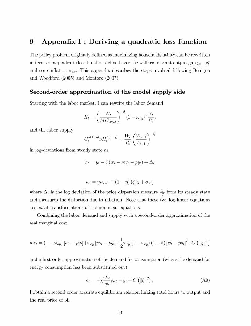
9 Appendix I : Deriving a quadratic loss function

The policy problem originally defined as maximizing households utility can be rewritten

in terms of a quadratic loss function defined over the welfare relevant output gap yt−y∗tand core inflation πy,t. This appendix describes the steps involved following Benigno

and Woodford (2005) and Montoro (2007).

Second-order approximation of the model supply side

Starting with the labor market, I can rewrite the labor demand

Ht =

µWt

MCtpy,t

¶−δ(1− ωoy)

δ YtP ∗t,

and the labor supply

Cσ(1−η)t νH

φ(1−η)t =

Wt

Pt

µWt−1Pt−1

¶−ηin log-deviations from steady state as

ht = yt − δ (wt −mct − pyt) +∆t

wt = ηwt−1 + (1− η) (φht + σct)

where ∆t is the log deviation of the price dispersion measure 1P∗tfrom its steady state

and measures the distortion due to inflation. Note that these two log-linear equations

are exact transformations of the nonlinear equations.

Combining the labor demand and supply with a second-order approximation of the

real marginal cost

mct = (1− fωoy) [wt − pyt]+fωoy [pot − pyt]+1

2fωoy (1− fωoy) (1− δ) [wt − pot]

2+O¡kξk3¢

and a first-order approximation of the demand for consumption (where the demand for

energy consumption has been substituted out)

ct = −χfωoc

sypo,t + yt +O

¡kξk2¢ , (A0)

I obtain a second-order accurate equilibrium relation linking total hours to output and

the real price of oil

33

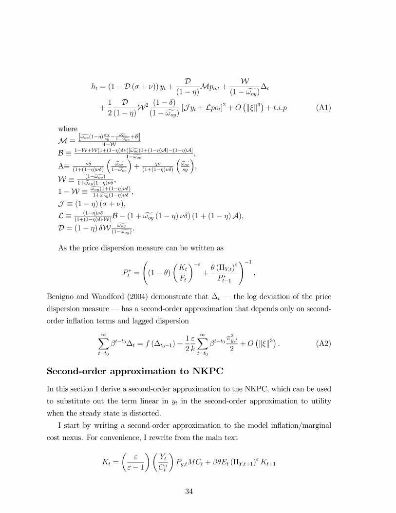
ht = (1−D (σ + ν)) yt +D

(1− η)Mpo,t +

W(1− fωoy)

∆t

+1

2

D(1− η)

W2 (1− δ)

(1− fωoy)[J yt + Lpot]2 +O

¡kξk3¢+ t.i.p (A1)

where

M ≡ [ωoc(1−η)σχsy− ωoc1−ωoc+B]

1−WB ≡ 1−W+W(1+(1−η)δν)[ωoc(1+(1−η)A)−(1−η)A]

1−ωoc ,

A≡ νδ(1+(1−η)νδ)

³ωoc1−ωoc

´+ χσ

(1+(1−η)νδ)³ωocsy

´,

W ≡ (1−ωoy)1+ωoy(1−η)νδ ,

1−W ≡ ωoy(1+(1−η)νδ)1+ωoy(1−η)νδ ,

J ≡ (1− η) (σ + ν),

L ≡ (1−η)νδ(1+(1−η)δνW)

B − (1 + fωoy (1− η) νδ) (1 + (1− η)A),D = (1− η) δW ωoy

(1−ωoy) .

As the price dispersion measure can be written as

P ∗t =

Ã(1− θ)

µKt

Ft

¶−ε+

θ (ΠY,t)ε

P ∗t−1

!−1,

Benigno and Woodford (2004) demonstrate that ∆t – the log deviation of the price

dispersion measure – has a second-order approximation that depends only on second-

order inflation terms and lagged dispersion

∞Xt=t0

βt−t0∆t = f (∆t0−1) +1

2

ε

k

∞Xt=t0

βt−t0π2y,t2+O

¡kξk3¢ . (A2)

Second-order approximation to NKPC

In this section I derive a second-order approximation to the NKPC, which can be used

to substitute out the term linear in yt in the second-order approximation to utility

when the steady state is distorted.

I start by writing a second-order approximation to the model inflation/marginal

cost nexus. For convenience, I rewrite from the main text

Kt =

µε

ε− 1¶µ

YtCσt

¶Py,tMCt + βθEt (ΠY,t+1)

εKt+1

34

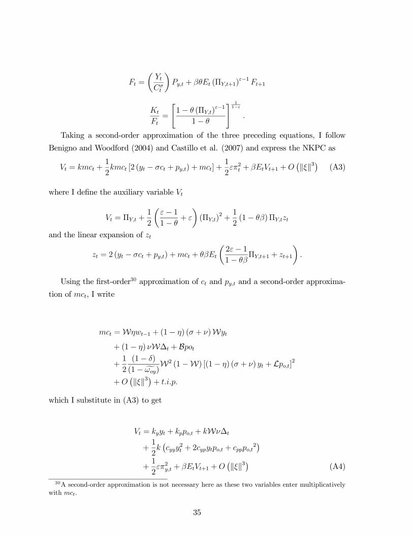
Ft =

µYtCσt

¶Py,t + βθEt (ΠY,t+1)

ε−1 Ft+1

Kt

Ft=

"1− θ (ΠY,t)

ε−1

1− θ

# 11−ε

.

Taking a second-order approximation of the three preceding equations, I follow

Benigno and Woodford (2004) and Castillo et al. (2007) and express the NKPC as

Vt = kmct +1

2kmct [2 (yt − σct + py,t) +mct] +

1

2επ2t + βEtVt+1 +O

¡kξk3¢ (A3)

where I define the auxiliary variable Vt

Vt = ΠY,t +1

2

µε− 11− θ

+ ε

¶(ΠY,t)

2 +1

2(1− θβ)ΠY,tzt

and the linear expansion of zt

zt = 2 (yt − σct + py,t) +mct + θβEt

µ2ε− 11− θβ

ΠY,t+1 + zt+1

¶.

Using the first-order30 approximation of ct and py,t and a second-order approxima-

tion of mct, I write

mct =Wηwt−1 + (1− η) (σ + ν)Wyt

+ (1− η) νW∆t + Bpot+1

2

(1− δ)

(1− fωoy)W2 (1−W) [(1− η) (σ + ν) yt + Lpo,t]2

+O¡kξk3¢+ t.i.p.

which I substitute in (A3) to get

Vt = kyyt + kppo,t + kWν∆t

+1

2k¡cyyy

2t + 2cypytpo,t + cpppo,t

2¢

+1

2επ2y,t + βEtVt+1 +O

¡kξk3¢ (A4)

30A second-order approximation is not necessary here as these two variables enter multiplicativelywith mct.

35

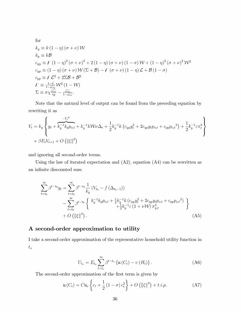
for

ky ≡ k (1− η) (σ + ν)Wkp ≡ kBcyy ≡ z (1− η)2 (σ + ν)2 + 2 (1− η) (σ + ν) (1− σ)W + (1− η)2 (σ + ν)2W2

cyp ≡ (1− η) (σ + ν)W (Σ+ B)−z (σ + ν) (1− η)L+ B (1− σ)

cpp ≡ zL2 + 2ΣB + B2z ≡ 1−δ

1−ωoyW2 (1−W)Σ ≡ σχωoc

sy− ωoc

1−ωoc .

Note that the natural level of output can be found from the preceding equation by

rewriting it as

Vt = ky

⎧⎪⎨⎪⎩yt +

−Y Ntz |

k−1y kppo,t + k−1y kWν∆t +1

2k−1y k

¡cyyy

2t + 2cypytpo,t + cpppo,t

2¢+1

2k−1y επ2t

⎫⎪⎬⎪⎭+ βEtVt+1 +O

¡kξk3¢and ignoring all second-order terms.

Using the law of iterated expectation and (A2), equation (A4) can be rewritten as

an infinite discounted sum

∞Xt=t0

βt−t0yt =∞Xt=t0

βt−t01

ky(Vt0 − f (∆t0−1))

−∞Xt=t0

βt−t0½

k−1y kppo,t +12k−1y k (cyyy

2t + 2cypytpo,t + cpppo,t

2)+12k−1y ε (1 + νW)π2y,t

¾+O

¡kξk3¢ . (A5)

A second-order approximation to utility

I take a second-order approximation of the representative household utility function in

to

Uto = Eto

∞Xt=to

βt−to u (Ct)− υ (Ht) . (A6)

The second-order approximation of the first term is given by

u (Ct) = Cuc

½ct +

1

2(1− σ) c2t

¾+O

¡kξk3¢+ t.i.p. (A7)

36

Substituting (A0) and its square into (A7), I get

u (Ct) = Cuc

½uyyt +

1

2uyyy

2t + uypytpo,t

¾+O

¡kξk3¢+ t.i.p. (A8)

for uy ≡ 1, uyy ≡ 1− σ, uyp ≡ −χωocsy(1− σ) and t.i.p stands for terms independent of

policy.

The second term in household utility is approximated by

v (Ht) = Hvh

½ht +

1

2(1 + ν)h2t

¾+O

¡kξk3¢+ t.i.p. (A9)

Substituting (A1) and its square in (A9) and getting rid of variables independent

of policy, I obtain

v (Ht) = Hvh

½vyyt + v∆∆t +

1

2vyyy

2t + vyppo,tyt

¾+O

¡kξk3¢+ t.i.p. (A10)

for

vy ≡ 1−D (ν + σ),

v∆ ≡ W1−ωoy ,

vyy ≡ D(1−η)W2 (1−δ)

(1−ωoy)J 2 + (1 + ν) (1−D (ν + σ))2

vyp ≡ D(1−η)

h(1 + ν) (1−D (ν + σ))M+W2 (1−δ)

(1−ωoy)JLi.

Now, since the technology is constant returns to scale, the share of labor in total

cost is equivalent to its share in marginal cost and the following equilibrium relationship

at the steady state

Y ucMC (1− fωoy) = Hvh,

which can be used to rewrite total utility Ut0 by substituting (A10) and (A8) into (A6),

to get

Ut0 = (Y uc)Eto

∞Xt=t0

βt−t0½uyyt +

1

2uyyy

2t + uyppo,tyt +

1

2uππ

2t

¾+O

¡kξk3¢+ t.i.p.,

(A11)

37

where

uy =CY−MC (1− fωoy) vy,

uyy =CY(1− σ)−MC (1− fωoy) vyy,

uyp = −CY

³ωocsy

´χ (1− σ)−MC (1− fωoy) vyp

u∆ = −MC (1− fωoy) v∆ = −MCWuπ =

εku∆ =

εkMCW.

For the last step, substituting the expression (A5) forP∞

t=t0βt−t0yt in (A11) obtains

Ut0 = −Y ucEto

∞Xt=t0

βt−t01

2

¡uyk

−1y kcyy − uyy

¢y2t

+1

2

¡2uyk

−1y kcyp − 2uyp

¢ytpo,t

+1

2

¡uyk

−1y ε (1 + νW)− uπ

¢π2t +O

¡kξk3¢+ t.i.p.,

that can be rewritten equivalently as

Ut0 = −Y ucEto

∞Xt=t0

βt−t01

2

¡uyk

−1y kcyy − uyy

¢[yt − y∗t ]

2

+1

2

¡uyk

−1y ε (1 + νW)− uπ

¢π2t +O

¡kξk3¢+ t.i.p.

which ends up as the central banks’s loss function to minimize

Ut0 = ΥEt0∞Xt=t0

βt−t0©λx2t + π2y,t

ª+O

¡kξk3¢+ t.i.p.

forΥ ≡ 12λπyY uc , Ψ ≡ kuyk

−1y cyp−uyp

kuyk−1y cyy−uyy , and where λ ≡

λyλπy

for λy = uyk−1y kcyy − uyy and

λπy = uyk−1y ε (1 + φW)−uπ. The output gap xt = yt−y∗t is now the percent deviation

of output with respect to the welfare relevant output y∗t itself defined as

y∗t ≡ −kuyk

−1y cyp − uyp

kuyk−1y cyy − uyypo,t = −Ψpot.

The values of λy and λπy are functions of the model parameters and describe the

weights assigned by the central bank to stabilize the welfare relevant output gap and

core inflation. In what follows I summarize this information with λ ≡ λyλπy, which

determines how concerned about the output gap a central bank should be after an

oil price shock. Typically, λ decreases with the sacrifice ratio and the degree of price

stickiness.

38

10 Appendix II: Characterizing optimal policy

Following Woodford (2003)31, I circumvent the usual time consistency issues associated

with fully optimal monetary policies by assuming that the central bank is able to

commit with full credibility to an optimal policy plan which specifies a full set of

state-contingent sequences xt, πy,t∞t=0 that minimize

ΥEt0∞Xt=t0

βt−t0©λx2t + π2y,t

ªsubject to the following sequence of constraints

πy,t = βEtπy,t+1 + kyxt + μt (A21)

and a constraint on the initial inflation rate

πy,t0 = πy,t0 , (A22)

where πy,t0 is defined as the inflation rate in time t0 that is consistent with optimal

policy in a "timeless perspective" or, in other words, the inflation rate that would have

been chosen a long time ago and which is consistent with the optimal precommitment

plan.

Solving this problem under the timeless perspective gives rise to the following set

of first-order conditions

xt = xt−1 − kyλπy,t, (A23)

which are supposed to hold for all t = 0, 1, 2, 3, . . . and which characterize the central

bank’s optimal policy response.

As shown in Section 3, acknowledging the low level of short-term substitutability

between oil and other factors gives rise to a cyclical distortion coming from the inter-

action between the steady-state efficiency distortion and the oil price shock. In terms

of the model equations, this cyclical distortion is translated into a cost-push shock that

enters the New Keynesian Phillips curve (NKPC henceforth).

Taking a log-linear approximation of equation (19) around the zero inflation steady-

state yields the standard result that (core) inflation is a function of next period inflation

and this period real marginal cost: the NKPC

πy,t = βEtπy,t+1 + kmct, (A24)

31See Woodford (2003), chapter 7 for a discussion.

39

where mct is the log-deviation of real marginal cost from its (distorted) steady state

and k =¡1−θθ

¢(1− θβ) is the elasticity of inflation to the real marginal cost.

Substituting the labor market clearing level of the real wage into the real marginal

cost equation (16), we can rewrite (A24) as

πy,t = βEtπy,t+1 + kygapt, (A25)

where the output gap gapt = yt − yNt measures the deviation between current output

and the natural level of output, and where

yNt = −kBky

pot, (A26)

for B a decreasing function of δ and χ, the oil production and consumption elasticitiesof substitution defined in Appendix I.

But (A25) can be equivalently rewritten as

πy,t = βEtπy,t+1 + kyxt + μt, (A27)

for μt = ky¡y∗t − yNt

¢the cost-push shock that arises as a direct function of the cyclical

wedge between the natural and the welfare maximizing level of output.

Obviously, the divine coincidence obtains when y∗t = yNt , which is the case for

χ = δ = 1, as shown in Section 3.

Appendix III : Deriving an optimal simple rule

In the timeless perspective equilibrium, inflation and the output gap behave according

to the rational expectation solution of the model consisting of the NKPC (A27) and

the policy rule (A23). Following McCallum (1999b) and McCallum and Nelson (2004),

the (no bubble) MSV solution takes the following form:

πy,t = α11xt−1 + α12μt (A31)

xt = α21xt−1 + α22μt, (A32)

where αij for i, j = 1, 2 are functions of β, ky and λ.

Because the supply of oil is supposed perfectly elastic at a given exogenous real

price, one can write the following definitions:

40

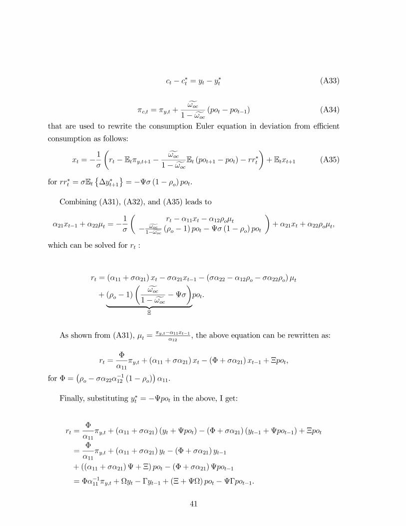
ct − c∗t = yt − y∗t (A33)

πc,t = πy,t +fωoc

1− fωoc(pot − pot−1) (A34)

that are used to rewrite the consumption Euler equation in deviation from efficient

consumption as follows:

xt = −1σ

µrt − Etπy,t+1 − fωoc

1− fωocEt (pot+1 − pot)− rr∗t

¶+ Etxt+1 (A35)

for rr∗t = σEt©∆y∗t+1

ª= −Ψσ (1− ρo) pot.

Combining (A31), (A32), and (A35) leads to

α21xt−1 + α22μt = −1

σ

µrt − α11xt − α12ρoμt

− ωoc1−ωoc (ρo − 1) pot −Ψσ (1− ρo) pot

¶+ α21xt + α22ρoμt,

which can be solved for rt :

rt = (α11 + σα21)xt − σα21xt−1 − (σα22 − α12ρo − σα22ρo)μt

+ (ρo − 1)µ fωoc

1− fωoc−Ψσ

¶| z

Ξ

pot.

As shown from (A31), μt =πy,t−α11xt−1

α12, the above equation can be rewritten as:

rt =Φ

α11πy,t + (α11 + σα21)xt − (Φ+ σα21)xt−1 + Ξpot,

for Φ =¡ρo − σα22α

−112 (1− ρo)

¢α11.

Finally, substituting y∗t = −Ψpot in the above, I get:

rt =Φ

α11πy,t + (α11 + σα21) (yt +Ψpot)− (Φ+ σα21) (yt−1 +Ψpot−1) + Ξpot

=Φ

α11πy,t + (α11 + σα21) yt − (Φ+ σα21) yt−1

+ ((α11 + σα21)Ψ+ Ξ) pot − (Φ+ σα21)Ψpot−1

= Φα−111 πy,t + Ωyt − Γyt−1 + (Ξ+ΨΩ) pot −ΨΓpot−1.

41

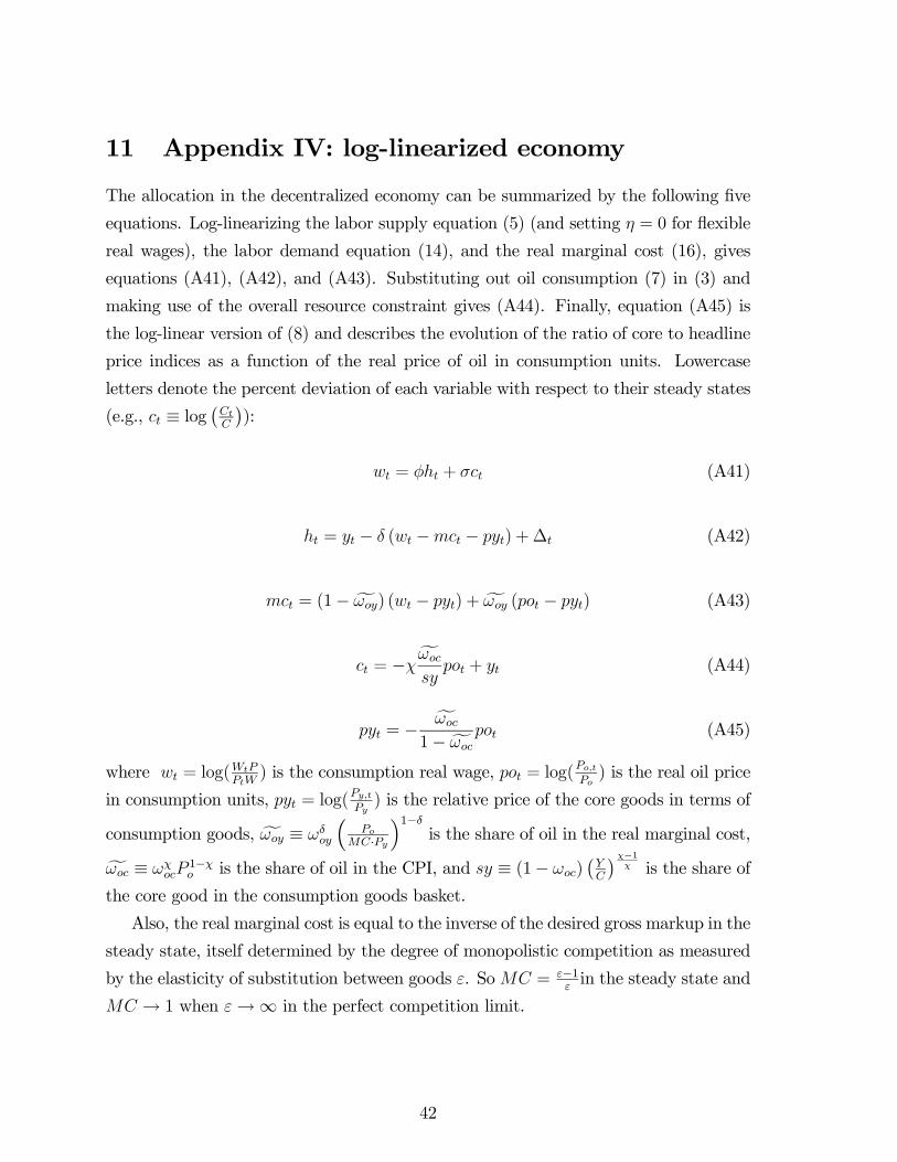
11 Appendix IV: log-linearized economy

The allocation in the decentralized economy can be summarized by the following five

equations. Log-linearizing the labor supply equation (5) (and setting η = 0 for flexible

real wages), the labor demand equation (14), and the real marginal cost (16), gives

equations (A41), (A42), and (A43). Substituting out oil consumption (7) in (3) and

making use of the overall resource constraint gives (A44). Finally, equation (A45) is

the log-linear version of (8) and describes the evolution of the ratio of core to headline

price indices as a function of the real price of oil in consumption units. Lowercase

letters denote the percent deviation of each variable with respect to their steady states

(e.g., ct ≡ log¡CtC

¢):

wt = φht + σct (A41)

ht = yt − δ (wt −mct − pyt) +∆t (A42)

mct = (1− fωoy) (wt − pyt) + fωoy (pot − pyt) (A43)

ct = −χfωoc

sypot + yt (A44)

pyt = − fωoc

1− fωocpot (A45)

where wt = log(WtPPtW

) is the consumption real wage, pot = log(Po,tPo) is the real oil price

in consumption units, pyt = log(Py,tPy) is the relative price of the core goods in terms of

consumption goods, fωoy ≡ ωδoy

³Po

MC·Py

´1−δis the share of oil in the real marginal cost,

fωoc ≡ ωχocP

1−χo is the share of oil in the CPI, and sy ≡ (1− ωoc)

¡YC

¢χ−1χ is the share of

the core good in the consumption goods basket.

Also, the real marginal cost is equal to the inverse of the desired gross markup in the

steady state, itself determined by the degree of monopolistic competition as measured

by the elasticity of substitution between goods ε. SoMC = ε−1εin the steady state and

MC → 1 when ε→∞ in the perfect competition limit.

42

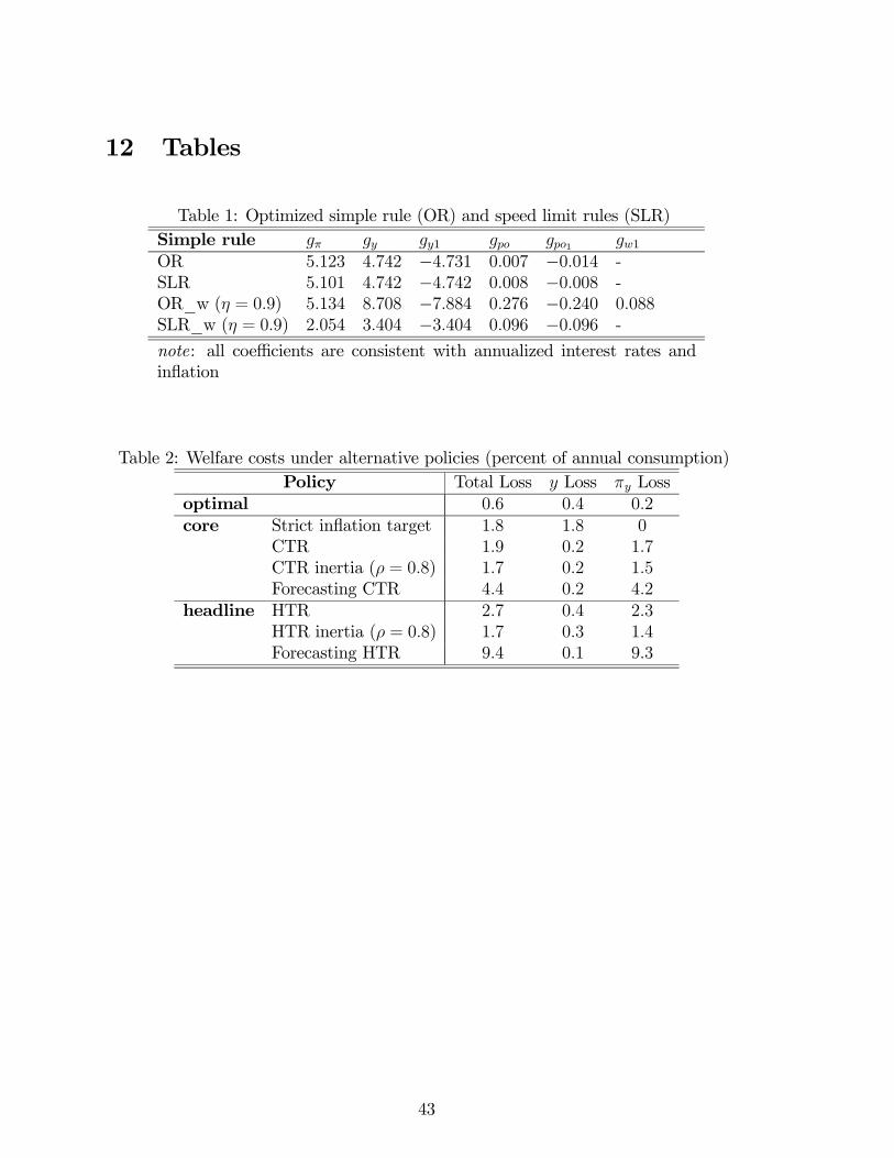
12 Tables

Table 1: Optimized simple rule (OR) and speed limit rules (SLR)Simple rule gπ gy gy1 gpo gpo1 gw1OR 5.123 4.742 −4.731 0.007 −0.014 -SLR 5.101 4.742 −4.742 0.008 −0.008 -OR_w (η = 0.9) 5.134 8.708 −7.884 0.276 −0.240 0.088SLR_w (η = 0.9) 2.054 3.404 −3.404 0.096 −0.096 -

note: all coefficients are consistent with annualized interest rates andinflation

Table 2: Welfare costs under alternative policies (percent of annual consumption)Policy Total Loss y Loss πy Loss

optimal 0.6 0.4 0.2core Strict inflation target 1.8 1.8 0

CTR 1.9 0.2 1.7CTR inertia (ρ = 0.8) 1.7 0.2 1.5Forecasting CTR 4.4 0.2 4.2

headline HTR 2.7 0.4 2.3HTR inertia (ρ = 0.8) 1.7 0.3 1.4Forecasting HTR 9.4 0.1 9.3

43

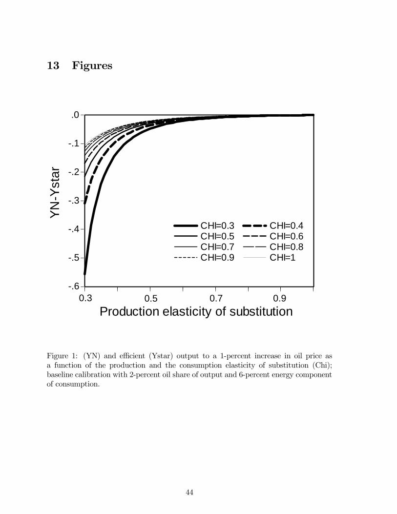
13 Figures

-.6

-.5

-.4

-.3

-.2

-.1

.0

CHI=0.3 CHI=0.4CHI=0.5 CHI=0.6CHI=0.7 CHI=0.8CHI=0.9 CHI=1

0.3 0.5 0.7 0.9Production elasticity of substitution

YN-Y

star

Figure 1: (YN) and efficient (Ystar) output to a 1-percent increase in oil price asa function of the production and the consumption elasticity of substitution (Chi);baseline calibration with 2-percent oil share of output and 6-percent energy componentof consumption.

44

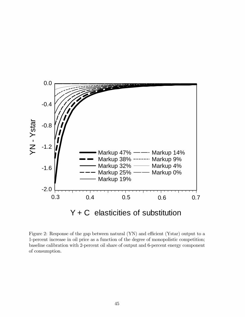
-2.0

-1.6

-1.2

-0.8

-0.4

0.0

Markup 47%Markup 38%Markup 32%Markup 25%Markup 19%

Markup 14%Markup 9%Markup 4%Markup 0%

0.3 0.4 0.5 0.6 0.7

Y + C elasticities of substitution

YN

- Y

star

Figure 2: Response of the gap between natural (YN) and efficient (Ystar) output to a1-percent increase in oil price as a function of the degree of monopolistic competition;baseline calibration with 2-percent oil share of output and 6-percent energy componentof consumption.

45

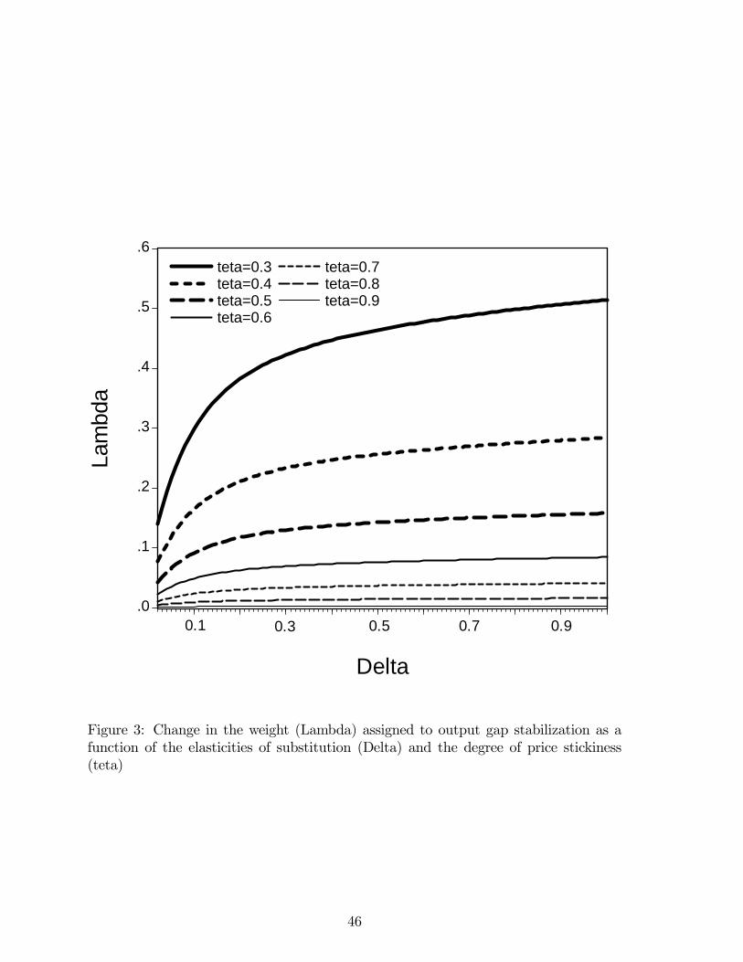
.0

.1

.2

.3

.4

.5

.6teta=0.3teta=0.4teta=0.5teta=0.6

teta=0.7teta=0.8teta=0.9

Lam

bda

Delta

0.1 0.50.3 0.7 0.9

Figure 3: Change in the weight (Lambda) assigned to output gap stabilization as afunction of the elasticities of substitution (Delta) and the degree of price stickiness(teta)

46

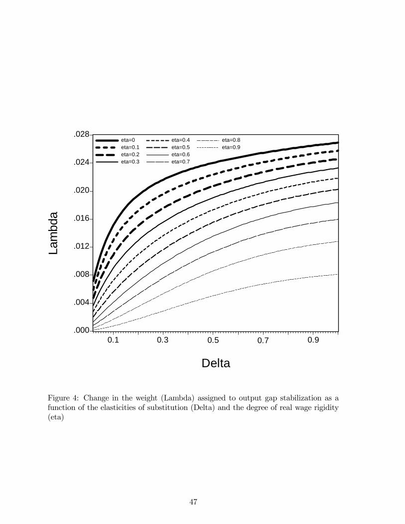
.000

.004

.008

.012

.016

.020

.024

.028eta=0eta=0.1eta=0.2eta=0.3

eta=0.4eta=0.5eta=0.6eta=0.7

eta=0.8eta=0.9

Lam

bda

0.1 0.3 0.5 0.7 0.9

Delta

Figure 4: Change in the weight (Lambda) assigned to output gap stabilization as afunction of the elasticities of substitution (Delta) and the degree of real wage rigidity(eta)

47

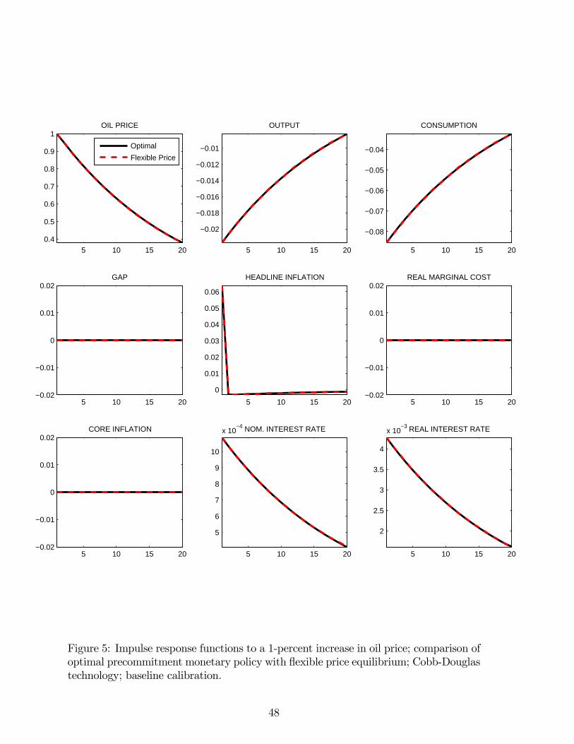
5 10 15 20

0.4

0.5

0.6

0.7

0.8

0.9

1OIL PRICE

Optimal

Flexible Price

5 10 15 20

−0.02

−0.018

−0.016

−0.014

−0.012

−0.01

OUTPUT

5 10 15 20

−0.08

−0.07

−0.06

−0.05

−0.04

CONSUMPTION

5 10 15 20−0.02

−0.01

0

0.01

0.02GAP

5 10 15 20

0

0.01

0.02

0.03

0.04

0.05

0.06

HEADLINE INFLATION

5 10 15 20−0.02

−0.01

0

0.01

0.02REAL MARGINAL COST

5 10 15 20−0.02

−0.01

0

0.01

0.02CORE INFLATION

5 10 15 20

5

6

7

8

9

10

x 10−4 NOM. INTEREST RATE

5 10 15 20

2

2.5

3

3.5

4

x 10−3 REAL INTEREST RATE

Figure 5: Impulse response functions to a 1-percent increase in oil price; comparison ofoptimal precommitment monetary policy with flexible price equilibrium; Cobb-Douglastechnology; baseline calibration.

48

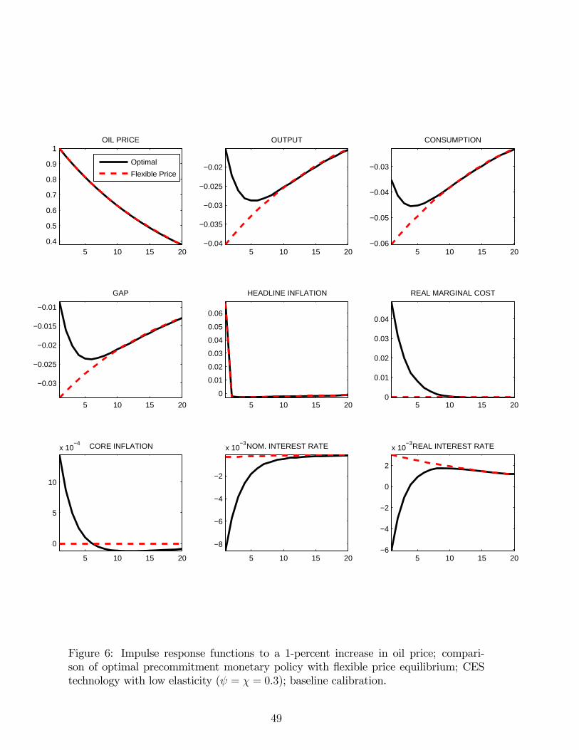
5 10 15 200.4

0.5

0.6

0.7

0.8

0.9

1OIL PRICE

Optimal

Flexible Price

5 10 15 20−0.04

−0.035

−0.03

−0.025

−0.02

OUTPUT

5 10 15 20−0.06

−0.05

−0.04

−0.03

CONSUMPTION

5 10 15 20

−0.03

−0.025

−0.02

−0.015

−0.01

GAP

5 10 15 20

0

0.01

0.02

0.03

0.04

0.05

0.06

HEADLINE INFLATION

5 10 15 200

0.01

0.02

0.03

0.04

REAL MARGINAL COST

5 10 15 20

0

5

10

x 10−4 CORE INFLATION

5 10 15 20

−8

−6

−4

−2

x 10−3NOM. INTEREST RATE

5 10 15 20−6

−4

−2

0

2

x 10−3REAL INTEREST RATE

Figure 6: Impulse response functions to a 1-percent increase in oil price; compari-son of optimal precommitment monetary policy with flexible price equilibrium; CEStechnology with low elasticity (ψ = χ = 0.3); baseline calibration.

49

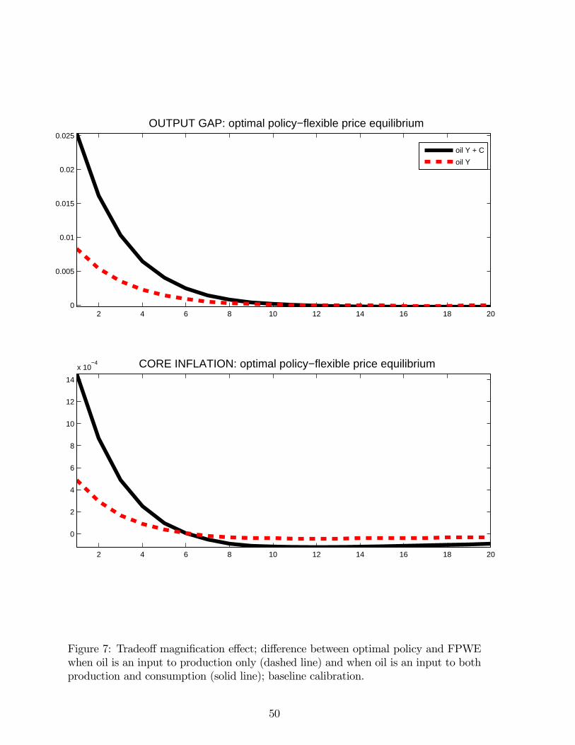
2 4 6 8 10 12 14 16 18 200

0.005

0.01

0.015

0.02

0.025

OUTPUT GAP: optimal policy−flexible price equilibrium

2 4 6 8 10 12 14 16 18 20

0

2

4

6

8

10

12

14

x 10−4 CORE INFLATION: optimal policy−flexible price equilibrium

oil Y + C

oil Y

Figure 7: Tradeoff magnification effect; difference between optimal policy and FPWEwhen oil is an input to production only (dashed line) and when oil is an input to bothproduction and consumption (solid line); baseline calibration.

50

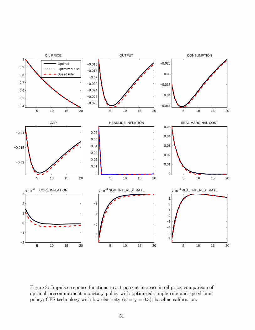
5 10 15 20

0.4

0.5

0.6

0.7

0.8

0.9

1OIL PRICE

Optimal

Optimized rule

Speed rule

5 10 15 20

−0.028

−0.026

−0.024

−0.022

−0.02

−0.018

−0.016

OUTPUT

5 10 15 20

−0.045

−0.04

−0.035

−0.03

−0.025

CONSUMPTION

5 10 15 20

−0.02

−0.015

−0.01

GAP

5 10 15 20

0

0.01

0.02

0.03

0.04

0.05

0.06

HEADLINE INFLATION

5 10 15 200

0.01

0.02

0.03

0.04

0.05REAL MARGINAL COST

5 10 15 20−2

−1

0

1

2

3x 10

−3 CORE INFLATION

5 10 15 20

−8

−6

−4

−2

x 10−3 NOM. INTEREST RATE

5 10 15 20

−6

−5

−4

−3

−2

−1

0

1

x 10−3 REAL INTEREST RATE

Figure 8: Impulse response functions to a 1-percent increase in oil price; comparison ofoptimal precommitment monetary policy with optimized simple rule and speed limitpolicy; CES technology with low elasticity (ψ = χ = 0.3); baseline calibration.

51

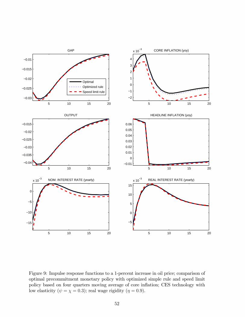
5 10 15 20

−0.03

−0.025

−0.02

−0.015

−0.01

GAP

Optimal

Optimized rule

Speed limit rule

5 10 15 20

−2

−1

0

1

2

3

4

x 10−3 CORE INFLATION (yoy)

5 10 15 20

−0.04

−0.035

−0.03

−0.025

−0.02

−0.015

OUTPUT

5 10 15 20−0.01

0

0.01

0.02

0.03

0.04

0.05

0.06

HEADLINE INFLATION (yoy)

5 10 15 20

−15

−10

−5

0

x 10−3 NOM. INTEREST RATE (yearly)

5 10 15 20

−5

0

5

10

15

x 10−3 REAL INTEREST RATE (yearly)

Figure 9: Impulse response functions to a 1-percent increase in oil price; comparison ofoptimal precommitment monetary policy with optimized simple rule and speed limitpolicy based on four quarters moving average of core inflation; CES technology withlow elasticity (ψ = χ = 0.3); real wage rigidity (η = 0.9).

52

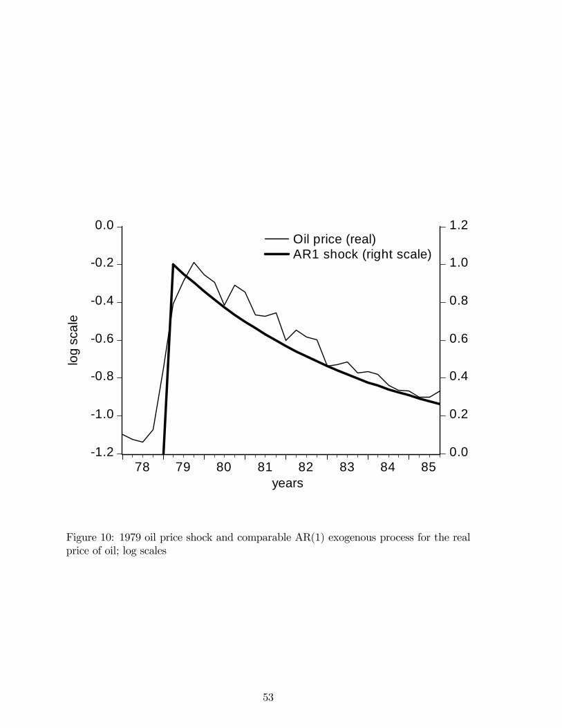
-1.2

-1.0

-0.8

-0.6

-0.4

-0.2

0.0

0.0

0.2

0.4

0.6

0.8

1.0

1.2

78 79 80 81 82 83 84 85

Oil price (real)AR1 shock (right scale)

years

log

scal

e

Figure 10: 1979 oil price shock and comparable AR(1) exogenous process for the realprice of oil; log scales

53

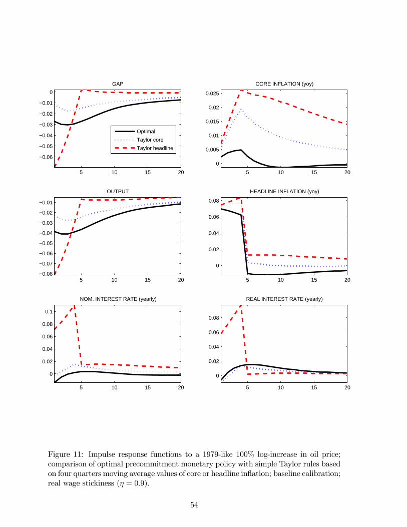
5 10 15 20

−0.06

−0.05

−0.04

−0.03

−0.02

−0.01

0

GAP

Optimal

Taylor core

Taylor headline

5 10 15 20

0

0.005

0.01

0.015

0.02

0.025

CORE INFLATION (yoy)

5 10 15 20−0.08

−0.07

−0.06

−0.05

−0.04

−0.03

−0.02

−0.01

OUTPUT

5 10 15 20

0

0.02

0.04

0.06

0.08

HEADLINE INFLATION (yoy)

5 10 15 20

0

0.02

0.04

0.06

0.08

0.1

NOM. INTEREST RATE (yearly)

5 10 15 20

0

0.02

0.04

0.06

0.08

REAL INTEREST RATE (yearly)

Figure 11: Impulse response functions to a 1979-like 100% log-increase in oil price;comparison of optimal precommitment monetary policy with simple Taylor rules basedon four quarters moving average values of core or headline inflation; baseline calibration;real wage stickiness (η = 0.9).

54

5 10 15 20−0.03

−0.025

−0.02

−0.015

−0.01

−0.005

0GAP

Optimal

Taylor core f.b.

Taylor head.f.b.

5 10 15 200

0.01

0.02

0.03

0.04

CORE INFLATION (yoy)

5 10 15 20−0.04

−0.035

−0.03

−0.025

−0.02

−0.015

−0.01

−0.005

OUTPUT

5 10 15 20

0

0.02

0.04

0.06

0.08

HEADLINE INFLATION (yoy)

5 10 15 20

−0.01

0

0.01

0.02

0.03

NOM. INTEREST RATE (yearly)

5 10 15 20

−5

0

5

10

15x 10

−3 REAL INTEREST RATE (yearly)

Figure 12: Impulse response functions to a 1979-like 100% log-increase in oil price;comparison of optimal precommitment monetary policy with simple forecast basedTaylor rules; baseline calibration; real wage stickiness (η = 0.9).

55

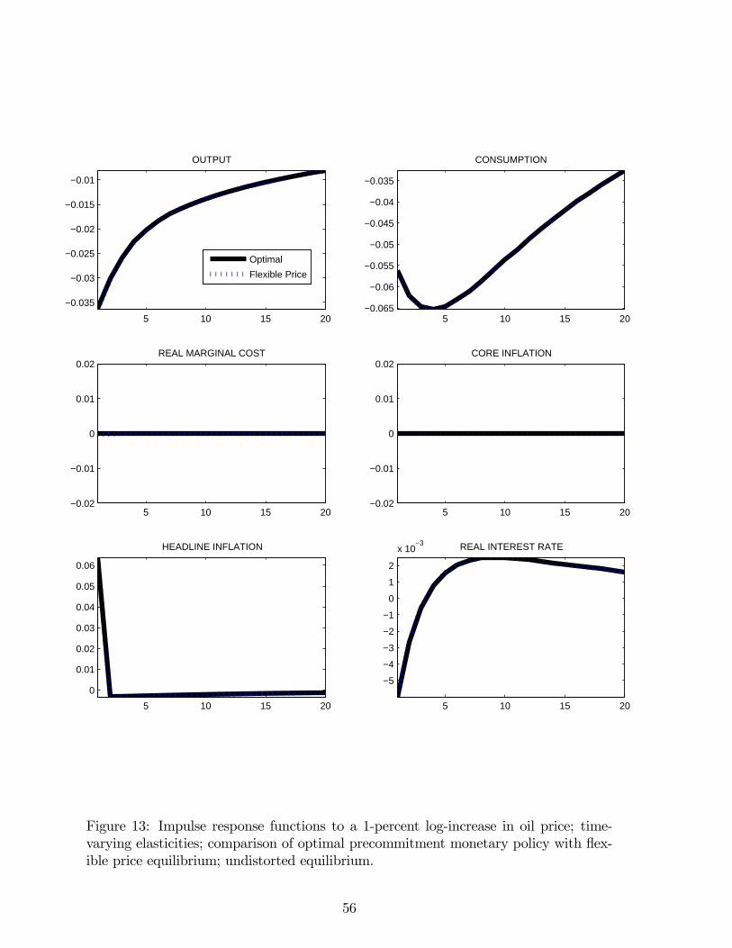
5 10 15 20

−0.035

−0.03

−0.025

−0.02

−0.015

−0.01

OUTPUT

Optimal

Flexible Price

5 10 15 20−0.065

−0.06

−0.055

−0.05

−0.045

−0.04

−0.035

CONSUMPTION

5 10 15 20−0.02

−0.01

0

0.01

0.02REAL MARGINAL COST

5 10 15 20−0.02

−0.01

0

0.01

0.02CORE INFLATION

5 10 15 20

0

0.01

0.02

0.03

0.04

0.05

0.06

HEADLINE INFLATION

5 10 15 20

−5

−4

−3

−2

−1

0

1

2

x 10−3 REAL INTEREST RATE

Figure 13: Impulse response functions to a 1-percent log-increase in oil price; time-varying elasticities; comparison of optimal precommitment monetary policy with flex-ible price equilibrium; undistorted equilibrium.

56

5 10 15 20

−0.03

−0.025

−0.02

−0.015

−0.01

OUTPUT

Optimal

Flexible Price

5 10 15 20

−0.06

−0.055

−0.05

−0.045

−0.04

−0.035

CONSUMPTION

5 10 15 20

0

0.005

0.01

0.015

0.02

0.025

0.03

0.035

REAL MARGINAL COST

5 10 15 20

−1

0

1

2

3

4

5

6x 10

−4 CORE INFLATION

5 10 15 20

0

0.01

0.02

0.03

0.04

0.05

0.06

HEADLINE INFLATION

5 10 15 20

−15

−10

−5

0

x 10−3 REAL INTEREST RATE

Figure 14: Impulse response functions to a 1-percent log-increase in oil price; Timevarying elasticities; comparison of optimal precommitment monetary policy with flex-ible price equilibrium; distorted equilibrium (markup 20%).

57