Monetary Policy, Trend Inflation and the Great Moderation: An Alternative Interpretation

Olivier Coibion College of William & Mary

Yuriy Gorodnichenko UC Berkeley and NBER

Draft: September 14th, 2009. Abstract: With positive trend inflation, the Taylor principle is not enough to guarantee a determinate equilibrium. We provide new theoretical results on restoring determinacy in New Keynesian models with positive trend inflation and combine these with new empirical findings on the Federal Reserve’s reaction function before and after the Volcker disinflation to find that 1) while the Fed likely satisfied the Taylor principle in the pre-Volcker era, the US economy was still subject to self-fulfilling fluctuations in the 1970s, 2) the US economy moved from indeterminacy to determinacy during the Volcker disinflation, and 3) the switch from indeterminacy to determinacy was due to the changes in the Fed’s response to macroeconomic variables and the decline in trend inflation during the Volcker disinflation.

Keywords: Trend inflation, Determinacy, Great Moderation, Monetary Policy JEL: C22, E3, E43, E5 We are grateful to Mark Gertler, three anonymous referees, Jean Boivin, Kathryn Dominguez, Jordi Gali, Pierre-Olivier Gourinchas, David Romer, and Carl Walsh, as well as seminar participants at the Bank of Canada, UC Berkeley, UC Santa Cruz, and SED for comments. We thank Eric Swanson for sharing the series of monetary policy surprises. We thank Jean Boivin for sharing his code. We thank Viacheslav Sheremirov for excellent research assistance. All errors are ours.

1  

I. Introduction

The pronounced decline in macroeconomic volatility since the early 1980s, frequently referred to as the Great

Moderation, has been the source of significant debate. One prominent explanation for this phenomenon is that

monetary policy became more “hawkish” with the ascent of Paul Volcker as Federal Reserve chairman in 1979.1

Originally proposed by Taylor (1999) and Clarida et al (2000), this view emphasizes that in the late 1960s and

1970s, the Fed systematically failed to respond sufficiently strongly to inflation, thereby leaving the US economy

subject to self-fulfilling expectations-driven fluctuations. The policy reversal enacted by Volcker and continued by

Greenspan—namely the increased focus on fighting inflation—stabilized inflationary expectations and removed this

source of economic instability.2 The theoretical argument is based on the Taylor principle: the idea that if the central

bank raises interest rates more than one for one with inflation, then self-fulfilling expectations will be eliminated as a

potential source of fluctuations. This intuitive concept is commonly used to differentiate between active (“hawkish”)

and passive (“dovish”) policy and is a hallmark of modern monetary policy. In addition, it has broad theoretical

support from standard New Keynesian models with zero trend inflation in which self-fulfilling expectations can

occur only when the Taylor principle is not followed, i.e. when monetary policy is passive.3 Yet point estimates of

the Fed’s response to inflation in the pre-Volcker era—regardless of whether they are less than one as in Clarida et al

(2000) or greater than one as in Orphanides (2004)—consistently come with such large standard errors that the issue

of whether the US economy was indeed in a state of indeterminacy, and hence subject to self-fulfilling fluctuations,

before Volcker remains unsettled.

In addition, recent theoretical work by Ascari and Ropele (2007), Kiley (2007) and Hornstein and Wolman

(2005) has cast additional doubt on the issue by uncovering an intriguing result: the Taylor principle breaks down

when trend inflation is positive (i.e., inflation rate in the steady state is positive). Using different theoretical

monetary models, these authors all find that achieving a unique Rational Expectations Equilibrium (REE) at

historically typical inflation levels requires much stronger responses to inflation than anything observed in empirical

estimates of central banks’ reaction functions. These results imply that the method of attempting to assess

determinacy solely through testing whether the central bank raises interest rates more or less than one for one with

inflation is inadequate: one must also take into account the level of trend inflation. For example, finding that the

Fed’s inflation response satisfied the Taylor principle after Volcker took office – as in Clarida et al (2000) – does not

necessarily imply that self-fulfilling expectations could not still occur since the inflation rate averaged around three

percent per year rather than the zero percent needed for the Taylor principle to apply. Similarly, the argument by

                                                            1 Other explanations emphasize inventory management or a change in the volatility of shocks. See Kahn et al (2002) for the former and Blanchard and Simon (2001) or Justiniano and Primiceri (2008) for examples of the latter. 2 This view has received recent support (see Lubik and Schorfheide (2004) and Boivin and Giannoni (2006)). On the other hand, Orphanides (2001, 2002, 2004) argues that once one properly accounts for the central bank’s real-time forecasts, monetary policy-makers in the pre-Volcker era responded to inflation in much the same way as those in the Volcker and Greenspan periods so self-fulfilling expectations could not have been the source of instability in the 1970s. 3 See Woodford (2003).

2  

Orphanides (2002) that monetary policy-makers satisfied the Taylor principle even before Volcker became chairman

does not necessarily invalidate the conclusion of Taylor (1999) and Clarida et al (2000) that the US economy moved

from indeterminacy to determinacy around the time of the Volcker disinflation: the same response to inflation by the

central bank can lead to determinacy at low levels of inflation but indeterminacy at higher levels of inflation. Thus,

it could be that the Volcker disinflation of 1979-1982, by lowering average inflation, was enough to shift the US

economy from indeterminacy to the determinacy region even with no change in the response of the central bank to

macroeconomic variables.

This paper offers two main contributions. First, we provide new theoretical results on the effects of

endogenous monetary policy for determinacy in New Keynesian models with positive trend inflation. Second, we

combine these theoretical results with empirical evidence on actual monetary policy to provide novel insight into

how monetary policy changes may have affected the stability of the US economy over the last forty years. For the

former, we build on the work of Ascari and Ropele (2007), Kiley (2007), and Hornstein and Wolman (2005) and

show that determinacy in New Keynesian models under positive trend inflation depends not just on the central

bank’s response to inflation and the output gap, as is the case under zero trend inflation, but rather is also a function

of many other components of endogenous monetary policy that are commonly found to be empirically important.

Specifically, we find that interest smoothing helps reduce the minimum long-run response of interest rates to

inflation needed to ensure determinacy. This differs substantially from the zero trend inflation case, in which inertia

in interest rate decisions has no effect on determinacy prospects conditional on the long-run response of interest rates

to inflation. We also find that price-level targeting helps achieve determinacy under positive trend inflation, even

when the central bank does not force the price level to fully return to its target path. Finally, while Ascari and

Ropele (2007) emphasize the potentially destabilizing role of responding to the output gap under positive trend

inflation, we show that responding to output growth can help restore determinacy for plausible inflation responses.

This finding provides new support for Walsh (2003) and Orphanides and Williams (2006), who call for monetary

policy makers to respond to output growth rather than the level of the output gap. More generally, we show that

positive trend inflation makes stabilization policy more valuable and calls for a more aggressive policy response to

inflation even if an economy stays in the determinacy region.

These results are not just theoretical curiosities since empirical work has found evidence for each of these

measures in monetary policy decisions. Interest smoothing is a particularly well-known empirical feature of interest-

rate decision-making.4 Gorodnichenko and Shapiro (2007) provide evidence for partial price-level targeting in the

US. Finally, Ireland (2004) finds that the Fed responds to both the output gap and output growth. Thus, given that

these policy actions are empirically and theoretically relevant, the key implication is that one cannot study the

determinacy prospects of the economy without considering simultaneously 1) the level of trend inflation, 2) the

                                                            4 See Clarida et al (2000) or Blinder and Reis (2005) for example.

3  

Fed’s response to inflation and its response to the output gap, output growth, price-level gap, and the degree of

interest smoothing, and 3) the model of the economy.

We revisit the issue of possible changes in monetary policy over the last forty years, as well as the

implications for economic stability, using a two-step approach. In the first step, we estimate the Fed’s reaction

function before and after the Volcker disinflation. We follow Orphanides (2004) and use the Greenbook forecasts

prepared by the Federal Reserve staff before each meeting of the Federal Open Market Committee (FOMC) as real-

time measures of expected inflation, output growth, and the output gap. Like the previous literature, we find

ambiguous results as to the hypothesis of whether the Taylor principle was satisfied before the Volcker disinflation

depending on the exact empirical specification, with large standard errors that do not permit us to clearly reject this

hypothesis. We also find that while the Fed’s long-run response to inflation is higher in the latter period, the

difference is not consistently statistically significant. Importantly, we uncover other ways in which monetary policy

has changed. First, the persistence of interest rate changes has gone up. Second, the Fed’s response to output growth

has gone up dramatically, while the response to the output gap decreased (although not statistically significantly).

These changes, according to our theoretical results, make determinacy a more likely outcome.

In the second step, we combine the empirical distribution of our parameter estimates of the Taylor rule with

a calibrated standard New Keynesian model and different estimates of trend inflation to infer the likelihood that the

US economy was in a determinate equilibrium each period. We find that despite the substantial uncertainty about

whether or not the Taylor principle was satisfied in the pre-Volcker era, the probability that the US economy was in

the determinacy region in the 1970s’s is zero according to our preferred empirical specification. This reflects the

combined effects of a response to inflation that was close to one, a non-existent response to output growth, relatively

little interest smoothing, and, most importantly, high trend inflation over this time period. On the other hand, given

the Fed’s response function since the early 1980s and the low average rate of inflation over this time period, 3%, we

conclude that the probability that the US economy has been in a determinate equilibrium since the Volcker

disinflation exceeds 99% according to our preferred empirical specification. Thus, we concur with the original

conclusion of Clarida et al (2000). However, whereas these authors reach their conclusion primarily based on testing

for the Taylor principle over each period, we argue that the switch from indeterminacy to determinacy was due to

several factors, none of which would likely have sufficed on their own. For example, taking the Fed’s pre-Volcker

response function and replacing any of the individual responses to macroeconomic variables with their post-1982

value would have had no effect on determinacy given the high average inflation rate in the 1970s. Instead, the most

important factors causing the switch away from indeterminacy were the higher inflation response combined the

decrease in the trend level of inflation.

Our paper is closely related to Cogley and Sbordone (2008). They find that controlling for trend inflation

has important implications in the estimation of the New Keynesian Phillips Curve, whereas we conclude that

accounting for trend inflation is necessary to properly assess the effectiveness of monetary policy in stabilizing the

economy. In a sense, one may associate the end of the Great Inflation as a source of the Great Moderation. To

4  

support this view, we estimate a time-varying parameter version of the Taylor rule from which we extract a measure

of time-varying trend inflation and therefore also a time series for the likelihood that the US economy was in the

determinacy region. This series indicates that the probability of determinacy went from 0% in 1980 to 90% in 1984,

which is the date most commonly associated with the start of the Great Moderation (McConnell and Perez-Quirós,

(2000)). To further support this notion, we document robust cross-country empirical evidence supporting a positive

link between trend inflation and GDP volatility. Devoting more effort to understanding the determinants of trend

inflation, as in Sargent (1999), Primiceri (2006) or Ireland (2007), and the Volcker disinflation of 1979-1982 in

particular, is likely to be a fruitful area for future research.

While our baseline results indicate that the US economy has most likely been within the determinacy region

since the Volcker disinflation, we also find that higher levels of trend inflation such as those reached in the 1970s

could bring the US economy to the brink of the indeterminacy region. In our counterfactual experiments, we find

that the complete elimination of the Fed’s current response to the output gap would remove virtually any chance of

indeterminacy, even at 1970s levels of inflation. But this does not imply that central banks should, in general, not

respond to the real side of the economy. The last result holds only because, since Volcker, the Fed has been

responding strongly to output growth. Were the Fed to stop responding to both the output gap and output growth,

indeterminacy at higher inflation rates would become an even more likely outcome.

Our approach is also very closely related to Lubik and Schorfheide (2004) and Boivin and Giannoni (2006).

Both papers address the same question of whether the US economy has switched from indeterminacy to determinacy

because of monetary policy changes, and both reach the same conclusion as us. However, our approaches are quite

different. First, we emphasize the importance of allowing for positive trend inflation, whereas their models are based

on zero-trend-inflation approximations.5 Thus, their models do not take into account the effects on determinacy of

the lower trend inflation brought about by the Volcker disinflation. Second, we consider a larger set of policy

responses for the central bank, which we argue has significant implications for determinacy as well.6 Third, we

estimate the parameters of the Taylor rule using real-time Fed forecasts, whereas these papers impose rational

expectations on the central bank in their estimation. Fourth, we allow for time-varying parameters in the Taylor rule

as well as time-varying trend inflation. Finally, we draw our conclusions about determinacy by feeding our

empirical estimates of the Taylor rule into a pre-specified model, whereas they estimate the structural parameters of

the DSGE model jointly with the Taylor rule. The pros and cons of the latter are well-known: greater efficiency in

estimation as long as the model is specified correctly. However, if any part of the model is misspecified, this can

                                                            5 In the case of Lubik and Schorfheide (2004), they use the standard NKPC expressed in terms of deviations from a non-zero trend inflation. This is equivalent to using a Calvo pricing model in which non-reoptimized prices are fully indexed to trend inflation. This eliminates all of the determinacy implications of positive trend inflation, as described in section 4.3. 6 For example, neither Lubik and Schorfheide (2004) nor Boivin and Giannoni (2006) allow for a response to output growth in the Taylor rule.

5  

affect all of the other estimated parameters.7 Our approach instead allows us to estimate the parameters of the Taylor

rule using real-time data while imposing as few restrictions as possible. We are then free to consider the

implications of these parameters for any model.8 While much more flexible than estimating a DSGE model, our

approach does have two key limitations. First, we are forced to select rather than estimate some parameter values for

the model. Second, because we do not estimate the shock processes, we cannot quantify the effect of our results as

completely as in a fully specified and estimated DSGE model.

The paper is structured as follows. Section 2 presents the model, while section 3 presents new theoretical

results on determinacy under positive trend inflation. Section 4 presents our Taylor rule estimates and their

implications for US determinacy since the 1970s, as well as robustness exercises. Section 5 concludes.

II. Model

We rely on a standard New Keynesian model, in which we focus on allowing for positive trend inflation. We use the

model to illustrate the importance of positive trend inflation for determinacy of REE and point to mechanisms that

can enlarge or reduce the region of determinacy for various policy rules.

2.1 The Model

The representative consumer maximizes expected utility over consumption (C) and labor (N),

1

Note that labor is provided individually to a continuum of industries. The budget constraint at time t+j is given by

where S is the stock of bonds held, W(i) is the nominal wage paid by sector i, P is the price index of the consumption

good, R is the nominal interest rate, and T is a lump-sum transfer from ownership of firms. The first order conditions

for the consumer are given by

/

1

                                                            7 Estimation of DSGE models under indeterminacy also raises additional issues such as selecting one of many equilibrium outcomes. 8 For example, while our baseline model relies on Calvo (1983) price setting, we can just as easily apply our Taylor rule estimates to a model with staggered price setting (as in Taylor (1977)), which we do in section 4.5. This is not the case using an estimated DSGE model, knowing that the estimated Taylor rule coefficients are sensitive to the price-setting assumptions of the model.

6  

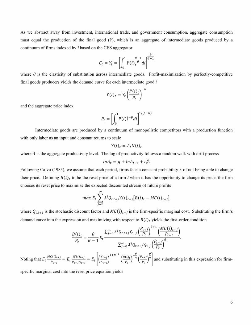
As we abstract away from investment, international trade, and government consumption, aggregate consumption

must equal the production of the final good (Y), which is an aggregate of intermediate goods produced by a

continuum of firms indexed by i based on the CES aggregator

where θ is the elasticity of substitution across intermediate goods. Profit-maximization by perfectly-competitive

final goods producers yields the demand curve for each intermediate good i

and the aggregate price index

/

Intermediate goods are produced by a continuum of monopolistic competitors with a production function

with only labor as an input and constant returns to scale

where A is the aggregate productivity level. The log of productivity follows a random walk with drift process

.

Following Calvo (1983), we assume that each period, firms face a constant probability of not being able to change

their price. Defining to be the reset price of a firm i when it has the opportunity to change its price, the firm

chooses its reset price to maximize the expected discounted stream of future profits

, .

where , is the stochastic discount factor and is the firm-specific marginal cost. Substituting the firm’s

demand curve into the expression and maximizing with respect to yields the first-order condition

1

∑ ,

∑ ,

.

Noting that and substituting in this expression for firm-

specific marginal cost into the reset price equation yields

7  

/

1

∑ ,

∑ ,

.

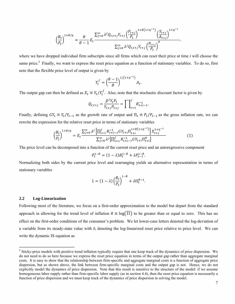
where we have dropped individual firm subscripts since all firms which can reset their price at time t will choose the

same price.9 Finally, we want to express the reset price equation as a function of stationary variables. To do so, first

note that the flexible price level of output is given by

1 /

.

The output gap can then be defined as / . Also, note that the stochastic discount factor is given by

, .

Finally, defining / as the growth rate of output and Π / as the gross inflation rate, we can

rewrite the expression for the relative reset price in terms of stationary variables

/ ∑ ∏ Π

∑ ∏ Π 1

The price level can be decomposed into a function of the current reset price and an autoregressive component

1 .

Normalizing both sides by the current price level and rearranging yields an alternative representation in terms of

stationary variables

1 1 Π .

2.2 Log-Linearization

Following most of the literature, we focus on a first-order approximation to the model but depart from the standard

approach in allowing for the trend level of inflation log Π to be greater than or equal to zero. This has no

effect on the first-order conditions of the consumer’s problem. We let lower-case letters denoted the log-deviation of

a variable from its steady-state value with bt denoting the log-linearized reset price relative to price level. We can

write the dynamic IS equation as

                                                            9 Sticky-price models with positive trend inflation typically require that one keep track of the dynamics of price dispersion. We do not need to do so here because we express the reset price equation in terms of the output gap rather than aggregate marginal costs. It is easy to show that the relationship between firm-specific and aggregate marginal costs is a function of aggregate price dispersion, but as shown above, the link between firm-specific marginal costs and the output gap is not. Hence, we do not explicitly model the dynamics of price dispersion. Note that this result is sensitive to the structure of the model: if we assume homogeneous labor supply rather than firm-specific labor supply (as in section 4.4), then the reset price equation is necessarily a function of price dispersion and we must keep track of the dynamics of price dispersion in solving the model.

8  

and the link between output growth and the change in the output gap as

.

However, non-zero trend inflation has important effects on the linearization of the price-setting equations.

First, positive trend inflation 0 implies that reset prices (relative to price level) will, on average, be higher than

the average price level

1 Π1

as long as the elasticity of substitution is greater than 1. This reflects the fact that a fixed reset price will erode in

real terms because of inflation. This implies that (log-linearized) inflation becomes less sensitive to changes in the

(log-linearized) relative reset price

1 ΠΠ

because, on average, firms who change prices set them above the average price level and therefore account for a

smaller share of expenditures than others.

More importantly for determinacy issues, the reset price equation is also sensitive to trend inflation. The

log-linearized version of equation (1) is

1 1 1

1 1

where Π and Π / .10 Note that under zero-trend inflation, . Consider how positive

trend inflation affects the relative reset price. First, higher trend inflation raises , so that the weights in the output

gap term shift away from the current gap and more towards future output gaps. This reflects the fact that as the

relative reset price falls over time, the firm’s future losses will tend to grow very rapidly. Thus, a sticky-price firm

must be relatively more concerned with marginal costs far in the future when trend inflation is positive. Second, the

relative reset price now depends on the discounted sum of future differences between output growth and interest

rates. Note that this term disappears when 0. This factor captures the scale effect of aggregate demand in the

future. The higher aggregate demand is expected to be in the future, the bigger the firm’s losses will be from having

a deflated price. The interest rate captures the discounting of future gains. When 0, these two factors cancel out

on average. Positive , however, induces the potential for much bigger losses in the future which makes these

effects first-order. Thus, as with the output gap, positive trend inflation induces more forward-looking behavior on

                                                            10 Note that for the reset price to have a well-defined solution in the steady-state requires that 1. See Bakhshi et al (2007).

9  

the part of firms. Third, positive raises the coefficient on expected inflation. This reflects the fact that the higher

is expected inflation, the more rapidly the firm’s price will depreciate, the higher it must set its reset price. Thus,

positive trend inflation makes firms more forward-looking in their price-setting decisions by raising the importance

of future marginal costs and inflation, as well as by inducing them to also pay attention to future output growth and

interest rates.

The log-linearized reset price equation can also be rewritten in a more convenient form as

1 /

where the variables dt and et follow respectively

1 1 1 1

.

2.3 Calibration

Allowing for positive trend inflation increases the state space of the model and makes analytical solutions infeasible.

Thus, all of our determinacy results are numerical. We calibrate the model as follows. The Frisch labor supply

elasticity, η, is set to 1. We let β=0.99 and the steady-state growth rate of real GDP per capita be 1.5% per year

( 1.015 . ), which matches the U.S. rate from 1969 to 2002. The elasticity of substitution θ is set to 10, which

corresponds to a markup of 11%. This size of the markup is consistent with estimates presented in Burnside (1996)

and Basu and Fernald (1997). Finally, the degree of price stickiness ( ) is set to 0.55, which amounts to firms

resetting prices approximately every 7 months on average. This is midway between the micro estimates of Bils and

Klenow (2004), who find that firms change prices every 4 to 5 months, and those of Nakamura and Steinsson (2008),

who find that firms change prices every 9 to 11 months. We will investigate the robustness of our results to these

parameters in subsequent sections.

III. Equilibrium Determinacy under Positive Trend Inflation

To close the model, we need to specify how monetary policy-makers set interest rates. One common description is a

simple Taylor rule, expressed in log-deviations from steady-state values:

(2)

in which the central bank sets interest rates as a function of contemporaneous (j=0) or future (j>0) inflation.11 As

documented in Woodford (2003), such a rule, when applied to a model like the one presented here with zero trend

inflation, yields a simple and intuitive condition for the existence of a unique rational expectations equilibrium: π >

                                                            11 Our results for j = -1 are similar to results for j = 0 and hence are not reported.

10  

1.12 This result, commonly known as the Taylor Principle, states that central banks must raise interest rates by more

than one-for-one with (expected) inflation to eliminate the possibility of sunspot fluctuations.

Yet, as emphasized in Ascari and Ropele (2007), Kiley (2007), and Hornstein and Wolman (2005), the

Taylor principle loses its potency in environments with positive trend inflation. Panel A in Figure 1 presents the

minimum response of the central bank to inflation necessary to ensure the existence of a unique rational expectations

equilibrium for both contemporaneous (j = 0) and forward-looking (j = 1) Taylor rules.13 As found by Ascari and

Ropele (2007), Kiley (2007), and Hornstein and Wolman (2005), the basic Taylor principle breaks down when the

trend inflation rate rises. With a contemporaneous Taylor rule, after inflation exceeds 1.2 percent per year, the

minimum response needed by the central bank starts to rise. With trend inflation of 6 percent a year, as was the case

in the 1970s, the central bank would have to raise interest rates by almost ten times the increase in the inflation rate

to sustain a determinate REE. Using forward-looking Taylor rules, the results are even more dramatic. As soon as

trend inflation slightly exceeds 0 percent per year, the minimum response to inflation exceeds our maximum bound

of 20, implying that a determinate REE does not exist for plausible inflation responses even at very low inflation

rates. This finding is in line with Woodford (2003, p. 516) and others who report that purely forward-looking rules

may be more subject to indeterminacy.14 In our case, the breakdown of the basic Taylor principle is amplified

because of the growing importance of forward-looking behavior in price-setting when trend inflation rises. Note

that this result is not limited to Calvo pricing. Kiley (2007) and Hornstein and Wolman (2005) find similar results

using staggered contracts a la Taylor (1977).15

In the rest of this section, we investigate how modifications of the basic Taylor rule affect the prospects for a

determinate equilibrium under positive trend inflation. First, we reproduce the results of Ascari and Ropele (2007),

Kiley (2007), and Hornstein and Wolman (2005) that focus on adding a response to the output gap. Second, we

provide new results on the determinacy implications of responding to output growth and discuss the distinction

between responding to the theoretical output gap versus a trend measure of the output gap, as well as the distinction

between responding to the growth rate in output versus the growth rate in the output gap. Third, we provide new

results on the determinacy implications of adding inertia to the policy rule via an interest smoothing motive and via

price level targeting. Finally, we demonstrate that positive trend inflation generally requires stronger responses by

the central bank to achieve stabilization than under zero trend inflation within the determinacy region.

                                                            12 Forward-looking rules, j ≥ 1, typically also place a constraint on the maximum value of to sustain a unique REE. See Woodford (2003, chapter 4). 13 For simplicity, we focus on the minimum response of inflation necessary for a unique REE, and do not plot the maximum values typical in forward-looking responses. This is because these, when present, are always at levels far beyond anything seen in empirical estimates of Taylor rules. 14 Furthermore, Bullard and Mitra (2002) and Woodford (2003) show that making the response to expected inflation more aggressive can conflict with ensuring determinacy because there is an upper bound on how aggressive the response to inflation can be in the region of determinacy. This explains why stronger responses to expected inflation do not expand the region of determinacy in the forward-looking rule. 15 Appendix Figure A1 reproduces all of our theoretical findings on determinacy with staggered price setting (under the assumption that prices are set for 3 quarters), yielding qualitatively similar results.

11  

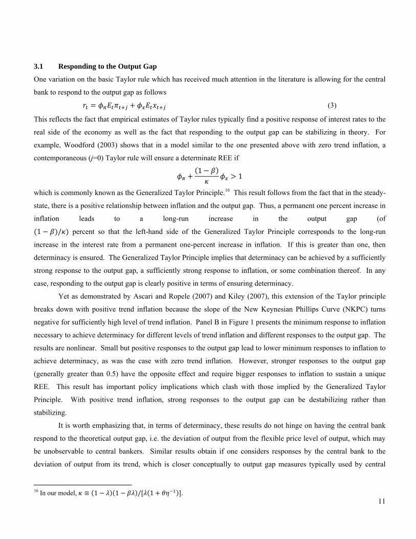
3.1 Responding to the Output Gap

One variation on the basic Taylor rule which has received much attention in the literature is allowing for the central

bank to respond to the output gap as follows

(3)

This reflects the fact that empirical estimates of Taylor rules typically find a positive response of interest rates to the

real side of the economy as well as the fact that responding to the output gap can be stabilizing in theory. For

example, Woodford (2003) shows that in a model similar to the one presented above with zero trend inflation, a

contemporaneous (j=0) Taylor rule will ensure a determinate REE if

11

which is commonly known as the Generalized Taylor Principle.16 This result follows from the fact that in the steady-

state, there is a positive relationship between inflation and the output gap. Thus, a permanent one percent increase in

inflation leads to a long-run increase in the output gap (of

1 / percent so that the left-hand side of the Generalized Taylor Principle corresponds to the long-run

increase in the interest rate from a permanent one-percent increase in inflation. If this is greater than one, then

determinacy is ensured. The Generalized Taylor Principle implies that determinacy can be achieved by a sufficiently

strong response to the output gap, a sufficiently strong response to inflation, or some combination thereof. In any

case, responding to the output gap is clearly positive in terms of ensuring determinacy.

Yet as demonstrated by Ascari and Ropele (2007) and Kiley (2007), this extension of the Taylor principle

breaks down with positive trend inflation because the slope of the New Keynesian Phillips Curve (NKPC) turns

negative for sufficiently high level of trend inflation. Panel B in Figure 1 presents the minimum response to inflation

necessary to achieve determinacy for different levels of trend inflation and different responses to the output gap. The

results are nonlinear. Small but positive responses to the output gap lead to lower minimum responses to inflation to

achieve determinacy, as was the case with zero trend inflation. However, stronger responses to the output gap

(generally greater than 0.5) have the opposite effect and require bigger responses to inflation to sustain a unique

REE. This result has important policy implications which clash with those implied by the Generalized Taylor

Principle. With positive trend inflation, strong responses to the output gap can be destabilizing rather than

stabilizing.

It is worth emphasizing that, in terms of determinacy, these results do not hinge on having the central bank

respond to the theoretical output gap, i.e. the deviation of output from the flexible price level of output, which may

be unobservable to central bankers. Similar results obtain if one considers responses by the central bank to the

deviation of output from its trend, which is closer conceptually to output gap measures typically used by central

                                                            16 In our model, 1 1 / 1 .

12  

bankers. Defining a new measure of trend output as the level of output that would occur if technology was equal

to its trend level ( )

1

then one can define an alternative measure of the gap as the deviation of output from its trend:

.

It follows that the theoretical output gap ( ), i.e. the deviation of output from its flexible price level, follows

where / is the deviation of technology from its trend.17

The only difference between the theoretical output gap and the gap relative to trend is the exogenous process

for technology . Thus, if we assume that the central bank responds to the trend measure of the gap , this will be

identical to having our original Taylor rule in which the central bank responds to the theoretical output gap ,

augmented with a response to technology. However, because the latter is exogenous and Woodford (2003) shows

that only the central bank’s response (or lack thereof) to endogenous variables matters for determinacy, it will have

no effect on determinacy. Thus, while the issue of whether the central bank responds to the theoretical output gap

or trend output gap will certainly matter for economic stabilization, it does not affect the determinacy regions.

3.2 Responding to Output Growth

The results for responding to the output gap under positive trend inflation call into question whether central banks

should be responding to the real side of the economy at all, even when one ignores the uncertainty regarding real-

time measurement of the output gap. Yet recent work by Walsh (2003) and Orphanides and Williams (2006) has

emphasized an alternative real variable that monetary policy makers can respond to for stabilization purposes: output

growth. This policy, sometimes referred to as a “speed limit”, has the advantage of greatly reducing measurement

issues since output growth is directly observable. To determine how such a policy might affect determinacy with

trend inflation, we consider the following Taylor rule

(4)

Panel C in Figure 1 presents the minimum response to inflation needed by the central bank to ensure

determinacy for different trend inflation rates and responses to output growth. For contemporaneous Taylor rules,

having the central bank respond to output growth helps ensure determinacy of the equilibrium, but this effect is much

weaker under forward-looking Taylor rules. The minimum level of inflation response needed for determinacy falls

as the response to output growth increases. In fact, a more general principle appears to be at work here: determinacy

                                                            17 Note that in our model technology follows a random walk process and hence technology does not deviate from trend. However, one may consider alternative processes such as ARI(1,1) or trend stationary technology so that at has meaningful variation.

13  

appears to be guaranteed for any positive trend inflation rate when the Fed responds to both inflation and current

output growth by more than one-for-one.

There are two channels through which responding to output growth helps achieve determinacy. First,

responding to the output growth rate effectively makes the policy reaction function history-dependent because it

responds to lagged output. Second, responding to output growth amplifies the central bank’s response to inflation.

To see this, consider a permanent increase in inflation . Substituting in for output growth using the dynamic IS

equation and re-arranging yields the following expression for real interest rates, assuming that 1,

11

.

Satisfying the Taylor principle, 1, ensures that the real interest rate rises with expected inflation. But, as

demonstrated in section 3.1, this is generally not sufficient to establish determinacy with positive trend inflation.

Allowing for a positive response to output growth, however, amplifies the magnitude of the response of real interest

rates to expected inflation. This is because when expected inflation rises, the real interest rate rises as long as

1. This causes output to fall but output growth is expected to rise via the dynamic IS equation (low but rising).

Higher expected output growth further raises the real interest rate when 0 which further lowers output and

raises expected output growth, etc. The size of the multiplier for the increase in real interest rates is given by

1/(1 ). As the central bank’s response to output growth approaches one, the multiplier approaches infinity.

This real interest rate multiplier effect partially accounts for why strong responses to output growth help restore

determinacy. Also note that similar to our results for the baseline Taylor rule with response only to inflation, making

the response to inflation more aggressive does not guarantee determinacy for forward-looking rules.

Overall, our findings suggest that targeting real variables is not automatically destabilizing under positive

trend inflation. Instead, strong responses to output growth help restore the basic Taylor principle whereas strong

responses to the output gap can be destabilizing. In addition, because output growth is readily observable and

subject to much less measurement error than the output gap, having the central bank follow a “speed limit” policy of

the type proposed by Walsh (2003) and Orphanides and Williams (2006) appears to be both feasible in real time and

helpful in diminishing the possibility of sunspot fluctuations.18

3.3 Interest Rate Smoothing

An additional extension to the basic Taylor rule which has become exceedingly common is allowing for interest

smoothing as follows

1 (5)                                                             18 While “speed limit” policies are sometimes expressed in terms of responses to the growth rate of the output gap rather than the growth rate of output, this distinction is irrelevant for determinacy issues. This is because the growth rate of the output gap is equal to the growth rate of output minus the innovation to technology. Thus, substituting the growth rate of the gap into the Taylor rule, then substituting out the growth in the gap with the growth in output yields an identical response of the central bank to endogenous variables, thereby yielding the same determinacy region. 

14  

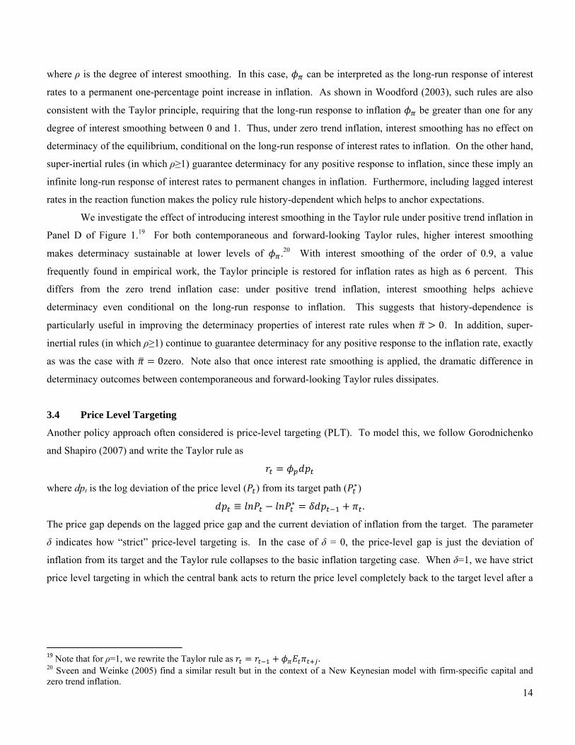
where ρ is the degree of interest smoothing. In this case, can be interpreted as the long-run response of interest

rates to a permanent one-percentage point increase in inflation. As shown in Woodford (2003), such rules are also

consistent with the Taylor principle, requiring that the long-run response to inflation be greater than one for any

degree of interest smoothing between 0 and 1. Thus, under zero trend inflation, interest smoothing has no effect on

determinacy of the equilibrium, conditional on the long-run response of interest rates to inflation. On the other hand,

super-inertial rules (in which ρ≥1) guarantee determinacy for any positive response to inflation, since these imply an

infinite long-run response of interest rates to permanent changes in inflation. Furthermore, including lagged interest

rates in the reaction function makes the policy rule history-dependent which helps to anchor expectations.

We investigate the effect of introducing interest smoothing in the Taylor rule under positive trend inflation in

Panel D of Figure 1.19 For both contemporaneous and forward-looking Taylor rules, higher interest smoothing

makes determinacy sustainable at lower levels of .20 With interest smoothing of the order of 0.9, a value

frequently found in empirical work, the Taylor principle is restored for inflation rates as high as 6 percent. This

differs from the zero trend inflation case: under positive trend inflation, interest smoothing helps achieve

determinacy even conditional on the long-run response to inflation. This suggests that history-dependence is

particularly useful in improving the determinacy properties of interest rate rules when 0. In addition, super-

inertial rules (in which ρ≥1) continue to guarantee determinacy for any positive response to the inflation rate, exactly

as was the case with 0zero. Note also that once interest rate smoothing is applied, the dramatic difference in

determinacy outcomes between contemporaneous and forward-looking Taylor rules dissipates.

3.4 Price Level Targeting

Another policy approach often considered is price-level targeting (PLT). To model this, we follow Gorodnichenko

and Shapiro (2007) and write the Taylor rule as

where dpt is the log deviation of the price level ( ) from its target path ( )

.

The price gap depends on the lagged price gap and the current deviation of inflation from the target. The parameter

δ indicates how “strict” price-level targeting is. In the case of δ = 0, the price-level gap is just the deviation of

inflation from its target and the Taylor rule collapses to the basic inflation targeting case. When δ=1, we have strict

price level targeting in which the central bank acts to return the price level completely back to the target level after a

                                                            19 Note that for ρ=1, we rewrite the Taylor rule as . 20 Sveen and Weinke (2005) find a similar result but in the context of a New Keynesian model with firm-specific capital and zero trend inflation.

15  

shock. The case of 0 < δ < 1 is “partial” price level targeting, in which the central bank forces the price level to

return only partway to the original target path.21

By quasi-differencing the Taylor rule after substituting in the price gap process, one can readily show that

this policy is equivalent to the following Taylor rule:

This is observationally equivalent to the Taylor rule with interest smoothing. Thus, when the central bank pursues

strict PLT (δ = 1), this is equivalent to the central bank having a super-inertial rule. Determinacy is therefore

guaranteed for any positive response to the price level (and therefore inflation). Thus, the result of Woodford (2003)

that strict PLT guarantees determinacy in a Calvo type model with zero trend inflation continues to hold (at least

numerically) under positive trend inflation. In addition, partial PLT (0<δ<1) will yield the exact same results as

interest smoothing. The stricter the PLT (the higher the δ), the smaller the long-run response to inflation will need to

be to sustain a determinate REE for positive trend levels of inflation.

3.5 Summary of Determinacy Results under Positive Trend Inflation

The fact that the basic Taylor principle breaks down with positive trend inflation raises important issues about

monetary policy. The first issue is whether there are other policy actions that can help ensure determinacy. Previous

work has shown that responding to the output gap can actually further destabilize the economy when trend inflation

is positive, eliminating one potential source of stability frequently utilized in theoretical and empirical work. Our

analysis shows three alternative policies which can help restore determinacy. Responding to output growth, rather

than the output gap, is one way that policy-makers can respond to the real side of the economy in a stabilizing

manner. Interest rate inertia and price level targeting are also useful in achieving determinacy for an economy with

positive trend inflation. The second issue is whether an economy is subject to sunspot equilibria depends not only on

the central bank’s response function but also on the level of trend inflation. Thus, a policy rule which is stabilizing

for one level of inflation may not be sufficient for determinacy at a higher level of inflation. In other words, changes

in the central bank’s inflation target can move an economy from determinacy to indeterminacy even with no change

in the central bank’s response to macroeconomic variables. Determinacy will therefore tend to be model specific and

sensitive to both the structure and parameters of the model. This implies that exercises focusing only on the inflation

response in a Taylor rule will in general be insufficient to answer whether this rule is consistent with a determinate

equilibrium.22

                                                            21 This could also be interpreted as targeting an average level of inflation. Suppose that the target for average inflation is 3% over 5 years. Then below-target inflation is later compensated with above target inflation. 22 Davig and Leeper (2007) argue that the possibility of the central banker switching to a policy rule consistent with determinacy (good policy) can lead to determinant outcomes even during times when the central banker’s policy rule is not sufficiently aggressive to guarantee determinacy (bad policy). In other words, the possibility of switching to the good policy mitigates the effects of the bad policy. However, Davig and Leeper observe that the bad policy will still lead to increased volatility of macroeconomic variables. Hence, we continue to associate periods of bad policy with periods of increased volatility.

16  

3.6 The Effects of Positive Trend Inflation on Economic Stabilization within the Determinacy Region

While all of our results have focused on the determinacy implications of positive trend inflation, one can also

consider the effects of trend inflation on economic stabilization within the determinacy region. Specifically, the

question we want to address is how strongly the central bank should respond to inflation under positive trend

inflation to achieve the same welfare from stabilization as under zero trend inflation. To assess the welfare gains due

to stabilization policies under zero and positive trend inflation, we derive the second order approximation to the

consumer utility function augmented with external habit formation in consumption when can differ from zero. 23,24

Proposition 1: The second order approximation to consumer utility

ln 1

is given by

11

1 var ,1

1 11

, ,1

1var

where , 1 Υ 1 Υ , , Υ 1 Υ , Υ log /

/ 1 , Π / 1 Π , h is the degree of habit formation in consumption, and Ht is the

exogenously determined (“external”) habit which is equal to lagged consumption.

Proof: see Appendix A.

It is straightforward to show that, for any plausible calibration of , , and , the weight on inflation

variability increases with the level of trend inflation . Hence, the central result of this proposition is that positive

trend inflation makes stabilization (specifically with respect to inflation) more valuable. This finding is intuitive: the

level of cross-sectional price dispersion increases with positive trend inflation and hence more variable inflation has

a larger effect on welfare.

                                                            23 Aruoba and Schorfheide (2009) investigate how trend inflation affects social welfare in a steady state. The first order effects documented in this paper are not dependent on our policy rules which are functions of deviations of inflation, output gap or any other relevant variable from a steady state. Hence, our analysis is more informative about the value of stabilization policies. Schmitt-Grohé and Uribe (2007) consider the benefits of stabilization policies with positive trend inflation. However, their calibration imposes that 80 percent of firms can reset prices every period and that the elasticity of demand is relatively low implying low strategic complementarity. With this calibration, positive trend inflation set at low levels as calibrated in Schmitt-Grohé and Uribe (2007) is not likely to lead to any significant departures from the standard Taylor principle, which is consistent with our robustness analysis below. Ascari and Ropele (2007) evaluate the effects of inflation and output gap variability given positive trend inflation. Our analysis is different in two key respects. First, they postulate a loss function rather than derive it as a second order approximation to consumer utility. Second, they consider policies under discretion or commitment while we analyze Taylor-type rules. 24 Note that the technology shock is the only economic disturbance in our model. Without habit formation, permanent innovations to the level of technology have no effects on inflation or the output gap. We also experimented with using transitory changes in technology and no habit formation and obtained qualitatively similar results.

17  

Using the second order approximation to consumer utility and the contemporaneous Taylor rule as in

equation (2), we can assess what policy response is required to maintain a fixed level of expected utility as trend

inflation increases.25 Let us define | , as the minimal policy response necessary to achieve utility level given

trend inflation . Figure 2 shows the ratio | , / | , for different where is equal to the level of utility a

policymaker can achieve with the lowest which yields determinacy at 6 percent trend inflation, the highest level

of trend inflation in our analysis. Irrespective of what degree of habit formation h we choose, the policymaker must

be increasingly aggressive to inflation as rises. We conclude that the key effect of positive trend inflation on

determinacy, i.e. requiring stronger responses to inflation by the central bank, also generally applies within the

parameter space in which determinacy occurs.

IV. Monetary Policy and Determinacy since the 1970s

In this section, we revisit the issue of how monetary policy may have changed before and after the Volcker

disinflation and whether any such changes may have moved the economy out of an indeterminate equilibrium in the

pre-Volcker era in light of how determinacy results hinge on the trend inflation rate. In section 4.1, we first estimate

policy reaction functions for each time period. We then feed the estimated parameters of the policy rules into our

model to assess the determinacy implications of the differences in response coefficients across the two periods given

different trend inflation rates in section 4.2. Section 4.3 considers counterfactual experiments to study which

changes in the policy rule have been most important and what further changes the Federal Reserve could pursue to

strengthen the prospects of achieving determinacy. In section 4.4, we allow for time-varying parameters in the

policy rule from which we can extract a time-varying measure of trend inflation. By combining our implied measure

of trend inflation and the time-varying parameters of the policy rule with our model, we construct a time series of the

probability of the US economy being in a state of determinacy since the late 1960s. In section 4.5, we investigate the

robustness of our baseline determinacy results to various price setting assumptions, the presence of habit formation,

and alternative measurement of the output gap. In section 4.6, we explore the correlation between volatility and

trend inflation using cross-country data.

Another way to explore the relationship between determinacy and policy would be to estimate the

parameters of the Taylor rule jointly with the structural parameters of the model using full-information methods.

This is the approach used by Lubik and Schorfheide (2004) and Boivin and Giannoni (2006). We chose not use this

approach for several reasons. First, our interest rate data and Greenbook forecasts are for each FOMC meeting,

making the time frequency of the interest rate rule inconsistent with that of other observable macroeconomic

variables and rendering simultaneous estimation particularly problematic. Second, our estimates of the Fed’s

reaction function are conditional on its historical forecasts, without requiring us to model how those forecasts are

                                                            25 When we compare utility for different levels of trend inflation, we focus only on the terms which depend on stabilization policies. We ignore the first order effects of trend inflation on welfare because they do not depend on stabilization policy.

18  

formed. Third, while full-information approaches are commonly applied to determinate equilibria, estimation under

indeterminacy requires selecting one out of many potential equilibrium outcomes. While various criteria can be used

for this selection, how best to proceed in this case remains a point of contention. Nonetheless, the fact that our

results point so strongly to indeterminacy in the pre-Volcker era provides support for recent work studying the

estimation of DSGE models under indeterminacy. Integrating positive trend inflation and monetary policy rules of

the type considered in this paper, along with (potentially) limited information on the part of the central bank, into a

DSGE model that can be estimated under determinacy and indeterminacy, while beyond the scope of this paper,

would be useful in quantifying the relative importance of the elimination of indeterminacy in accounting for the

Great Moderation.

4.1 Estimation of the Federal Reserve’s Reaction Function

Our baseline empirical specification for the Fed’s reaction function is a generalized Taylor rule in which we assume

there is a single break in trend inflation as well as in the coefficients of the response function around the time of the

Volcker disinflation. Our baseline period-specific estimated Taylor rule is thus

1 , (6)

where is an error term. This specification allows for interest smoothing of order two, as well as a response to

inflation, output growth, and the output gap. Allowing for responses to both the output gap and output growth is

necessary because the two have different implications for determinacy with positive trend inflation. The constant

term c consists of the steady-state level of interest rate, plus the (constant) level of trend inflation, as well as the

target levels of output growth and output gap. To estimate equation (6), we follow Orphanides (2004) and use real-

time data for the estimation. Specifically, we use the Greenbook forecasts of current and future macroeconomic

variables prepared by staff members of the Fed a few days before each meeting of the Federal Open Market

Committee (FOMC). The interest rate is the target federal funds rate set at each meeting, from Romer and Romer

(2004). The measure of the output gap is based on Greenbook forecasts, as compiled by Orphanides (2003, 2004).

Data is available from 1969 to 2002 for each official meeting of the FOMC. We consider two time samples: 1969-

1978 and 1983-2002. Thus, we drop the period from 1979-1982 in which the Federal Reserve officially abandoned

interest rate targeting in favor of targeting monetary aggregates. Each t is a meeting of the FOMC. From 1969-

1978, meetings were monthly, whereas from 1983 on, meetings were held every 6 weeks. Note that this implies that

the interest smoothing parameters in the Taylor rule are not directly comparable across the two time periods.26

                                                            26 Cochrane (2007) argues that the central bank’s response to inflation will be unidentified in New Keynesian models when the Taylor rule includes a stochastic intercept term that corresponds to the natural rate of interest, i.e. the rate of interest that would hold in the frictionless economy. However, Sims (2008) shows that Cochrane’s argument holds only if the central bank is responding one-for-one to fluctuations in the natural rate of interest, an unlikely scenario due to the inherent difficulty in measuring the natural rate of interest, particularly in real time. More generally, the Fed may be stabilizing inflation with off-equilibrium path threats that may not be observed in equilibrium. However, in practice, periods of apparent indeterminacy in the policy rule have come when trend inflation is high. Thus it is highly unlikely that the Fed has effectively been using off-equilibrium strategies over this period to stabilize inflation.

19  

Table 1 presents results of the least squares estimation of equation (6) over each time period for three cases:

contemporaneous Taylor rule, forward-looking Taylor rule, and mixed. In the case of the contemporaneous Taylor

rule, we use the central bank’s forecast of values for the current quarter. In the case of the forward-looking rule, we

use the forecast of the average value over the next two quarters (but three quarter ahead forecast for the output gap).

We find that interest rate decisions are best modeled (in terms of fitting the data) as a function of forecasts of future

inflation but forecasts of contemporaneous output gap and output growth rate.27 We will treat this as the baseline in

subsequent sections. In addition to point estimates, standard errors and selected statistics of fit, we report the sum of

the interest smoothing parameters converted to a quarterly frequency.28 We also include the probability value of the

null that each of the parameters and the sum of interest smoothing parameters are the same in the two periods.

We find that the Fed’s response to inflation in the pre-Volcker era satisfied the Taylor principle in forward-

looking specifications, but not under the contemporaneous Taylor rules. Because the forward-looking specification

is statistically preferred to a contemporaneous response to inflation, our evidence supports the argument of

Orphanides (2004) that the Fed satisfied the Taylor principle in both periods, albeit weakly so. Like Orphanides, we

also find that while our estimates consistently point to a stronger response by the Fed to inflation in the latter period,

we can only reject the null of no change in the response to inflation in the case of the mixed rule. Thus, our

estimates of the Fed’s response coefficients do not provide strong support for the claims of Taylor (1999) and

Clarida et al (2000) that the failure to satisfy the basic Taylor principle before Volcker placed the US economy in an

indeterminate region. However, we do find that other response coefficients have changed in statistically significant

ways. First, interest rate decisions have become more persistent, in the sense that the sum of the autoregressive

components is higher in the latter period than in the early period, and statistically significantly so in two out of three

specifications. Second, the Federal Reserve has changed how it responds to the real side of the economy. Whereas

the period before the Volcker disinflation was characterized by a strong long-run response to the output gap, but no

statistically discernible response to output growth, the period since the Volcker disinflation displays much stronger

long-run responses by the Fed to output growth than to the output gap.

These results illustrate an important feature of the data: monetary policy has changed across time, despite the

fact that one cannot consistently reject the null that the Fed’s response to inflation alone has not changed. Thus were

one to rely only on the basic Taylor principle as guidance for establishing determinacy, then one would reach the

same conclusion as Orphanides (2004). Yet the results of section 3 demonstrate that, once one allows for positive

trend inflation, all of the components of the Fed’s response function play a role, along with the parameters of the

model and the level of trend inflation. Thus, the changes in the Fed’s response to output growth and interest                                                             27 Specifically, we consider all possible variants of forward-looking and contemporaneous-looking for inflation, output gap, and output growth responses and use the AIC to select the best specification. In Appendix Table A3, we report AIC and BIC for different specifications. Note that the mixed rule used as our baseline calibration clearly dominates alternative specifications. 28 Because there is no convenient formula for converting AR(2) parameters from monthly or 6-weekly frequency to quarterly, we use the following approach: Given estimated AR(2) parameters, we simulate an AR(2) process at the original frequency, and then create a new (average) series at the quarterly frequency. We then regress the quarterly series on two lags of itself over a sample of 50,000 periods and report the sum of the estimated parameters.

20  

smoothing, along with the stronger response to inflation, each have consequences for determinacy. Interestingly, all

of the policy changes made by the Fed since the Volcker disinflation –stronger response to output growth and

inflation, more interest smoothing, and weaker response to output gap (albeit not statistically significantly so for the

latter)– will tend to make determinacy more likely.

Note that, as Orphanides (2001, 2004), Boivin (2006) and others argue, the key benefit of using Greenbook

forecasts is to properly condition on the Federal Reserve’s real-time information set. An additional appealing feature

of using Greenbook forecasts is that one does not need to impose rational expectations on the central bank to

estimate the reaction function. However, to estimate a Taylor rule such as (6) by least squares requires that the

orthogonality condition be satisfied, i.e. current forecasts be uncorrelated with the current monetary policy

innovation. We think there are several reasons why estimation by least squares is likely to be adequate. First, as

argued in Boivin (2006), if contemporaneous inflation, GDP growth and the output gap are unaffected by the current

monetary policy innovation, as commonly assumed in the VAR literature, then estimation of equation (6) using

contemporaneous values (j = 0) will be consistent.29 The validity of the exogeneity assumption can then be assessed

for rules with longer forecasting horizons by verifying whether coefficient estimates are sensitive to the forecasting

horizon or more formally by using the Hausman test to directly assess whether the exogeneity condition is violated.

We estimated a forward-looking Taylor rule using least squares and instrumental variables (IV) estimators, using

current forecasts of lagged variables as instruments (since these are orthogonal to current monetary policy

innovations) and found no evidence that favored IV estimation (Appendix Table A1). Second, if Greenbook

forecasts were made under assumptions about future policy actions that were systematically overturned, then these

forecasts would be inferior to those made by agents who made better projections of future policy actions, such as

professional forecasters. Yet Romer and Romer (2000) document that Greenbook forecasts of inflation

systematically outperform professional forecasters. Third, we can augment the right-hand-side of equation (6) with a

direct measure of monetary policy innovations from Gürkaynak, Sack and Swanson (2005), who identify monetary

policy innovations by comparing Fed Funds Futures markets predictions of FOMC decisions with actual decisions.

Adding this variable eliminates the omitted variable bias and hence least squares yields consistent estimates. We

found that estimates in this augmented specification are remarkably close to the specification without policy shocks

identified via Fed Funds Futures (see results in Appendix Table A2).30 We find similar results when we approximate

the policy innovations as the difference between the fed funds rate assumed in the Greenbook forecasts and the Fed

                                                            29 Estimates of the effects of monetary policy shocks indicate that these shocks have little to no effect on macroeconomic variables at short time horizons. This implies that the exogeneity assumption should also generally be valid when using forecasts of macroeconomic variables over the next one to two quarters, as emphasized in Romer and Romer (2004). 30 The variation in the error term remaining after including policy shocks can be interpreted in a variety of ways (e.g., as measurement errors). We note, however, that the size of the remaining variation is very small and, hence, differences in interpretation are not likely to quantitatively affect our results.

21  

Funds rate chosen by the FOMC.31,32 In summary, one may reasonably expect that the feedback from policy

surprises to regressors in the Taylor rule is likely to lead to negligible distortions in the least squares estimates.

4.2 Determinacy Before and After the Volcker Disinflation

To assess the implications of our estimated response functions, we feed the estimated parameters from each Taylor

rule into the model described and calibrated in section 2 to examine the determinacy implications of monetary policy

over the two samples. We first consider whether the model yields a determinate rational expectations equilibrium

(REE) given the estimated parameters of the Taylor rule for two trend inflation rates – 3% and 6% – designed to

replicate average inflation rates in each of the two time periods. In addition, we consider how determinacy varies

over the statistical distribution of our parameter estimates. For each type of Taylor rule and each sample period, we

draw 10,000 times from the distribution of the estimated parameters and assess the fraction of draws that yield a

determinate rational expectations equilibrium at 3% and 6% trend inflation. The results are presented in the bottom

panel of Table 1.33

First, we find that the pre-1979 response of the central bank implied an indeterminate REE given the average

inflation rate of that time (6%). This is a very robust implication of the Taylor rule estimates: both the

contemporaneous and mixed Taylor rules yield zero percent of draws consistent with determinacy while the forward-

looking rule delivers a probability of determinacy of only 12%, despite a point estimate of 1.75 for the Fed’s

response to expected inflation. On the other hand, the post-1982 response is consistent with a determinate REE at

the low average inflation rate of this period (3%). Using our preferred specification, the mixed Taylor rule, more

than 99% of the empirical distribution of parameters yields determinacy. Thus, like Taylor (1999), Clarida et al

(2000) and others, we find that monetary policy before Volcker led to indeterminacy in the 1970s, but that since

1982 the Fed’s response has helped ensure determinacy.

Our approach also allows us to assess the relative importance of the change in the Fed’s response function

versus the change in trend inflation for altering the determinacy status of the economy. For example, we note that

had the Fed maintained its pre-1979 response function but lowered average inflation from 6% to 3% per year (via a

change in the inflation target in the Taylor rule), the US economy would have remained in the indeterminacy region

of the parameter space. Thus, the Volcker disinflation, during which average inflation was brought down, would

have been insufficient to guarantee determinacy without a change in the Fed’s response function as well. Similarly,

we also find that the Fed’s response to macroeconomic variables since 1982, while consistent with determinacy at

                                                            31 The series for the path of the Fed Funds rate assumed in the Greenbook forecasts are available from the Real-Time Data Research Center at the Federal Research Bank of Philadelphia. 32 Unfortunately, the trading of Fed Funds Futures started in late 1980s and Fed Funds rate assumptions in Greenbook forecasts are available only after 1981 and thus we cannot investigate if these results extend prior to the 1980s. 33 Before feeding estimated parameters into the model, we first convert the interest smoothing parameter into a quarterly frequency using the same approach as described in footnote 28 and divide the coefficient on the output gap by four, since the Taylor rules are estimated using annualized rates, the Taylor rule in the model is written in terms of quarterly rates, and the output gap is scale invariant.

22  

3% trend inflation, is only marginally consistent with determinacy at the inflation rate of the 1970s. Specifically,

while the estimated parameters of each specification yield a determinate REE at 6% trend inflation, only sixty

percent of draws from the distribution of estimated parameters are consistent with determinacy at this inflation rate

according to the mixed Taylor rule estimates. Thus, the estimated parameters are near the edge of the parameter

space consistent with a unique REE. This implies that if the Fed in the 1970s had simply switched to the current

policy rule without simultaneously engaging in the Volcker disinflation, it is quite possible that the US economy

would have remained subject to self-fulfilling expectations-driven fluctuations. The shift from indeterminacy to

determinacy thus appears to have been due to two major policy changes: a change in the policy rule and a decline in

the inflation target of the Federal Reserve during the Volcker disinflation. Either one done individually would likely

have been insufficient to move the economy from indeterminacy to determinacy.

4.3 Counterfactual Experiments

The results of the previous section indicate that changes in monetary policy around the Volcker disinflation likely

moved the US economy from a state of indeterminacy to one of determinacy, as originally argued by Taylor (1999)

and Clarida et al (2000) and more recently reemphasized by Lubik and Schorfheide (2004) and Boivin and Giannoni

(2006). While previous work has focused almost exclusively on the Fed’s response to inflation, we have shown that

the Fed has also significantly changed its response to output growth as well as the degree of interest smoothing, but

also that changes in trend inflation have played a crucial role.

In this section, we perform counterfactual experiments designed to differentiate between the contributions of

each policy change for determinacy. To address the quantitative importance of each policy change, we consider the

following set of experiments. First, for each period’s policy rule, we draw from the empirical distribution of

estimated parameters and calculate the fraction of draws that yield a determinate equilibrium at 3% and 6% trend

inflation rates. This replicates the exercise in Table 1 and serves as the baseline for this section’s analysis. Then, we

repeat the procedure but switch, in turn, the period-specific coefficients on inflation, interest smoothing, output

growth and the output gap.34 We continue to use baseline parameter values for the rest of the model.

The results are presented in Table 2. Consider first the effect of switching . For the pre-1979 period at

6% trend inflation, this has no effect on determinacy, meaning that the fraction of draws from the empirical

distribution of parameter estimates yielding a determinate REE is essentially unchanged at 0%. This means that if

the only policy change enacted by the Fed had been to raise its response to inflation to the post-1982 level, but

leaving its other response coefficients and the trend inflation unchanged, the US economy would have remained in

an indeterminate equilibrium. Thus, while our findings support the argument of Clarida et al (2000) that the US

                                                            34 Specifically, we draw from each time period’s distribution of parameters, leaving the covariance matrix unchanged but altering the mean of the relevant parameter to match that of the other time sample. We assume a once and for all unexpected change in the parameters of the policy rule even though a more realistic description of policy changes would involve gradual transitions in parameter values (see Boivin 2006).

23  

moved from indeterminacy to determinacy during the Volcker disinflation, we emphasize not just the change in the

Fed’s response to inflation, which by itself was not enough to shift the US economy out of the indeterminacy of the

1970s, but rather that this policy change combined with the Volcker disinflation can account for much of the

movement away from indeterminacy. Specifically, we find that if the Fed had maintained its pre-Volcker policy rule

but used the post-1982 inflation response, then this single policy switch combined with the Volcker disinflation

would have raised the likelihood of determinacy to about two-thirds.

We also consider the implication of switching the degree of interest smoothing across periods and the

response to output growth, both of which are statistically different in the two time periods (see Table 1). For interest

smoothing, we find almost identical results as in the baseline case, indicating that the increased inertia of interest rate

decisions since the Volcker disinflation cannot account for the switch in determinacy across periods. Switching the

response to output growth across the two periods has a more important effect. If we start with the estimated post-

1982 policy reaction function and switch to its pre-1979 value, the fraction of draws yielding determinacy in the

post-1982 period at 3% (6%) trend inflation would have been only 91% (26%) instead of 99% (62%) if the response

to output growth had remained unchanged. On the other hand, starting from the pre-1979 policy rule and raising

the response to output growth to the post-1982 level has almost no effect on determinacy. This indicates that the

change in , the response to output growth, complemented the other policy changes in terms of restoring

determinacy, but could not, by itself, account for the reversal in determinacy around the time of the Volcker

disinflation.

Finally, we consider the effect of the decrease in the Fed’s response to the output gap, a policy difference

strongly emphasized by Orphanides (2004), although we cannot reject the null of no change in the Fed’s response to

the gap across time periods. We find that if the post-1982 Fed had responded as strongly to the output gap as they

did before Volcker, then the likelihood that the US economy would still be in the indeterminacy region would be

somewhat higher, particularly at higher rates of inflation. At 6% trend inflation, the fraction of draws yielding

determinacy goes from 62% to 33%. Thus, this result supports the emphasis placed by Orphanides (2004) on the

lower response to the output gap by the Fed since the Volcker era, but for a different reason. Orphanides stresses

that if the output gap is mismeasured in real-time, then a strong response to the output gap, like that followed by the

Fed in the 1970s, can be destabilizing. Our interpretation is instead that even if the output gap is perfectly measured

by the central bank, strong responses to the output gap can be destabilizing by raising the probability of

indeterminacy.

We can extend our analysis by investigating how the central bank can further minimize the likelihood of

indeterminacy. Thus, we consider determinacy prospects using each policy rule but imposing 0.35 In the post-

1982 period, eliminating the response to the output gap would raise the likelihood of determinacy significantly. This

                                                            35 Here, we draw from each period’s distribution of parameters, then impose that the relevant coefficient be exactly zero for each draw.

24  

is most clearly visible at the 6% inflation rate, when eliminating the Fed’s response to the output gap would raise the

probability of determinacy from 62% to 99%. Thus, while the Fed has improved determinacy prospects somewhat

by reducing its response to the output gap since the 1970s, a complete elimination of this response would be better

yet.

Importantly, this does not imply that the Federal Reserve is best served by not responding to the real side of

the economy. Consider the counterfactual of no response by the Fed to both the output gap and output growth in

each time period. In the post-1982 period, the prospects for determinacy are lower than in the case with just zero

response to output gap, particularly at higher inflation rates. For the latter, eliminating any response to the real side

of the economy yields determinacy in less than 13% of draws, instead of the 99% when only the response to the

output gap is eliminated. Thus, the current strong response to output growth by the Federal Reserve is well-justified,

and would play an important stabilizing role were the Fed to completely eliminate responding to the output gap.

Furthermore, a positive response to the real side of the economy should not necessarily be interpreted as central

bankers being ‘dovish’ on inflation.

4.3 Time-Varying Trend Inflation

Our baseline estimation approach assumes that trend inflation, as well as the central bank’s target for real GDP

growth and the output gap, is constant within each time period. In this section, we relax these assumptions and

extract a measure of trend inflation which allows us to calculate a time series for the probability of determinacy for

the U.S. economy. Our approach follows Boivin (2006), who estimates a similar Taylor rule with time-varying

coefficients. We generalize the Taylor rule in equation (6) to:

1 , , , , ,

, ,

where is the target rate of inflation, is the equilibrium real interest rate, is the target rate of growth of real

GDP, and is the target level of the output gap. We can rewrite this as

1 , , , , , , , (7)

where the time-varying constant term is given by

1 , , 1 , , , . (8)

To estimate the parameters of equation (7), we follow Boivin (2006) and assume that each of the parameters follows

a random walk process and allow for two breaks in the volatility of shocks to the parameters: 1979 and 1982. Using

the Kalman filter and the corresponding smoother, we construct time series of the response coefficients of the Taylor

rule and of the time-varying constant.

The results for the estimated parameters, including the time-varying constant, are presented in Figure 3,

along with one standard deviation confidence intervals. The results broadly confirm those in the baseline estimation:

namely, there was a sharp increase in the Fed’s response to inflation and output growth around the time of the

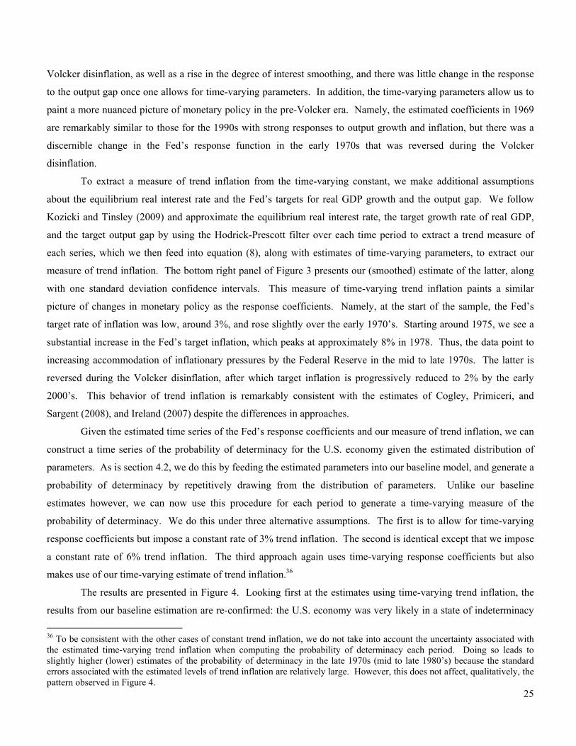
25  

Volcker disinflation, as well as a rise in the degree of interest smoothing, and there was little change in the response

to the output gap once one allows for time-varying parameters. In addition, the time-varying parameters allow us to

paint a more nuanced picture of monetary policy in the pre-Volcker era. Namely, the estimated coefficients in 1969

are remarkably similar to those for the 1990s with strong responses to output growth and inflation, but there was a

discernible change in the Fed’s response function in the early 1970s that was reversed during the Volcker

disinflation.

To extract a measure of trend inflation from the time-varying constant, we make additional assumptions

about the equilibrium real interest rate and the Fed’s targets for real GDP growth and the output gap. We follow

Kozicki and Tinsley (2009) and approximate the equilibrium real interest rate, the target growth rate of real GDP,

and the target output gap by using the Hodrick-Prescott filter over each time period to extract a trend measure of

each series, which we then feed into equation (8), along with estimates of time-varying parameters, to extract our

measure of trend inflation. The bottom right panel of Figure 3 presents our (smoothed) estimate of the latter, along

with one standard deviation confidence intervals. This measure of time-varying trend inflation paints a similar

picture of changes in monetary policy as the response coefficients. Namely, at the start of the sample, the Fed’s

target rate of inflation was low, around 3%, and rose slightly over the early 1970’s. Starting around 1975, we see a

substantial increase in the Fed’s target inflation, which peaks at approximately 8% in 1978. Thus, the data point to

increasing accommodation of inflationary pressures by the Federal Reserve in the mid to late 1970s. The latter is

reversed during the Volcker disinflation, after which target inflation is progressively reduced to 2% by the early

2000’s. This behavior of trend inflation is remarkably consistent with the estimates of Cogley, Primiceri, and

Sargent (2008), and Ireland (2007) despite the differences in approaches.

Given the estimated time series of the Fed’s response coefficients and our measure of trend inflation, we can

construct a time series of the probability of determinacy for the U.S. economy given the estimated distribution of

parameters. As is section 4.2, we do this by feeding the estimated parameters into our baseline model, and generate a

probability of determinacy by repetitively drawing from the distribution of parameters. Unlike our baseline

estimates however, we can now use this procedure for each period to generate a time-varying measure of the

probability of determinacy. We do this under three alternative assumptions. The first is to allow for time-varying

response coefficients but impose a constant rate of 3% trend inflation. The second is identical except that we impose

a constant rate of 6% trend inflation. The third approach again uses time-varying response coefficients but also

makes use of our time-varying estimate of trend inflation.36

The results are presented in Figure 4. Looking first at the estimates using time-varying trend inflation, the

results from our baseline estimation are re-confirmed: the U.S. economy was very likely in a state of indeterminacy

                                                            36 To be consistent with the other cases of constant trend inflation, we do not take into account the uncertainty associated with the estimated time-varying trend inflation when computing the probability of determinacy each period. Doing so leads to slightly higher (lower) estimates of the probability of determinacy in the late 1970s (mid to late 1980’s) because the standard errors associated with the estimated levels of trend inflation are relatively large. However, this does not affect, qualitatively, the pattern observed in Figure 4.

26  

before the Volcker disinflation but not thereafter. Again, the use of time-varying parameters provides a more

detailed perspective on the pre-Volcker era. At the start of our sample period, the probability of determinacy was

close to one, reflecting the low estimate of trend inflation at the time as well as the strong responses to inflation and

output growth. However, we can observe a rapid deterioration of stabilization properties of monetary policy in the

early 1970s, such that by 1975 the probability of the U.S. economy being in a state of determinacy was less than ten

percent. This was not reversed until the Volcker disinflation, since which the probability of determinacy has

consistently exceeded eighty percent. This finding is consistent with the view laid out in Romer and Romer (2002)

emphasizing that good policy prevailed during Martin’s chairmanship of the Fed (which ended in 1970) and returned

with Volcker’s ascent.

The results with time-varying parameters also confirm the key role played by changes in the level of trend

inflation in accounting for the apparent transition from determinacy to indeterminacy in the early 1970s and then

back to determinacy during the Volcker disinflation. Consider the first transition in the early 1970s. Our estimates

imply that if the Fed had only changed its response coefficients but held the target rate of inflation constant at 3%,

the economy would have been right at the edge of the determinacy-indeterminacy region, implying that the change in

trend inflation accounts for approximately half of the switch from determinacy to indeterminacy over this time

period. During the Volcker disinflation, the results are similar: had the Fed only changed its response coefficients

but left its target inflation in the neighborhood of six percent, the probability of indeterminacy would still have been

around fifty percent by the mid-1990s rather than ten percent. Thus, these results reinforce the key point that one

cannot address determinacy issues only by focusing on the response coefficients of the central bank, instead we need

to consider the interaction of the central bank’s response coefficients with trend inflation.

4.5 Robustness Analysis

The fact that higher trend inflation raises the likelihood of indeterminacy reflects the increased importance of

forward-looking behavior in firms’ price setting decisions. Specifically, when firms reset prices in the Calvo model,

the weight placed on future profits depends strongly on how likely a firm is to not have altered its price by that

period. Thus, greater price stickiness will naturally increase the sensitivity of reset prices to expectations of future

macroeconomic variables. As a result, one would expect indeterminacy to become increasingly difficult to eliminate

as the degree of price rigidity rises.

To see whether this is indeed the case, we consider two alternative degrees of price stickiness. First, we

follow Bils and Klenow (2004) who find that firms update prices every 4 to 5 months on average which corresponds

to =0.40 in our model. Second, we follow Nakamura and Steinsson (2008) who find much longer durations of price

spells ranging between 8 and 11 months on average. In this case, we set =0.70. We reproduce the determinacy

results of section 4.2 in Table 3 using the mixed Taylor rule for each time period. Under the Bils and Klenow case,

we recover our baseline results of indeterminacy in the 1970s but determinacy after the Volcker disinflation.

27  

However, we can see that determinacy is more easily sustained under lower levels of price rigidity by the fact that

the fraction of the empirical distribution yielding determinacy is consistently higher than in the baseline case. In

addition, using this lower rate of price-stickiness implies that determinacy would have been achieved solely through

the change in the Fed’s response to macroeconomic variables. Using the degree of price stickiness from Nakamura

and Steinsson moves all of the quantitative results in the opposite direction. For the pre-Volcker era, the results are

qualitatively similar to our baseline findings, with indeterminacy occurring consistently at both inflation rates.

However, with this higher degree of price stickiness, we now find that the current policy rule is likely inconsistent

with determinacy: even at 3% inflation, less than 50% of the empirical distribution of Taylor rule estimates yields a

determinate REE equilibrium.

Clearly, the degree of price stickiness plays an important role in determinacy conditions. However, the

importance of this variable is likely overestimated under Calvo pricing. This setup forces firms to place some weight

on possible future outcomes in which their relative price would be so unprofitable that “real world” firms would

likely choose to pay a menu cost and reset their price.37 An alternative approach to Calvo pricing is the staggered

contracts approach of Taylor (1977) in which firms set prices for a pre-determined duration of time. This pricing

assumption can loosely be thought of as a lower bound on forward-looking behavior (conditional on price durations)

since it imposes zero weight on expected profits beyond those of the contract length in the firm’s reset price

optimization. We replicate our results using staggered pricing with firms setting prices for three quarters and display

the results in Table 3. For the pre-Volcker era, the results again largely point to indeterminacy at high levels of

inflation. However, the post-1982 policy rule is now consistent with determinacy at both 3% and 6% inflation rates.

In fact, the results using staggered price setting with duration of 9 months are very close to those using Calvo price

setting with average price duration of 5 months. This reflects the shortened time horizon of price-setting firms with

staggered contracts and the concurrent decrease in the importance of expectations of future outcomes relative to the

Calvo case. We interpret Taylor pricing as setting a lower bound on determinacy issues (conditional on average

price durations) and Calvo pricing an upper bound. Despite the sensitivity of determinacy results to these variations,

what seems clear is that the U.S. economy was in an indeterminate region of the parameter space in the pre-Volcker

era given the high average inflation of that time, but moved into the determinacy region after 1982. The relative

importance of the decrease in trend inflation versus the changes in the Fed’s response to macroeconomic conditions,

on the other hand, is sensitive to the price-setting model and average price durations used. In the absence of

definitive evidence favoring one modeling approach over the other along with clearer results on how sticky prices

actually are in the data, we are unable to decisively measure the relative importance of these two monetary policy

changes.

A closely related issue is how to model price adjustment frictions faced by firms. The notion of menu costs

naturally gives rise to models in which firms change prices infrequently while the notion that firms face                                                             37 Another way to see this limitation of the Calvo model is to note that using Nakamura and Steinsson rates of price-setting, the Calvo model breaks down (i.e. γ2 ≥ 1) at an inflation rate of 6.1%.

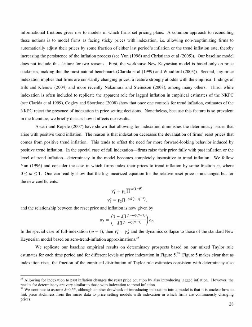
28  

informational frictions gives rise to models in which firms set pricing plans. A common approach to reconciling

these notions is to model firms as facing sticky prices with indexation, i.e. allowing non-reoptimizing firms to

automatically adjust their prices by some fraction of either last period’s inflation or the trend inflation rate, thereby

increasing the persistence of the inflation process (see Yun (1996) and Christiano et al (2005)). Our baseline model

does not include this feature for two reasons. First, the workhorse New Keynesian model is based only on price

stickiness, making this the most natural benchmark (Clarida et al (1999) and Woodford (2003)). Second, any price

indexation implies that firms are constantly changing prices, a feature strongly at odds with the empirical findings of

Bils and Klenow (2004) and more recently Nakamura and Steinsson (2008), among many others. Third, while

indexation is often included to replicate the apparent role for lagged inflation in empirical estimates of the NKPC

(see Clarida et al 1999), Cogley and Sbordone (2008) show that once one controls for trend inflation, estimates of the

NKPC reject the presence of indexation in price setting decisions. Nonetheless, because this feature is so prevalent

in the literature, we briefly discuss how it affects our results.

Ascari and Ropele (2007) have shown that allowing for indexation diminishes the determinacy issues that

arise with positive trend inflation. The reason is that indexation decreases the devaluation of firms’ reset prices that

comes from positive trend inflation. This tends to offset the need for more forward-looking behavior induced by

positive trend inflation. In the special case of full indexation—firms raise their price fully with past inflation or the

level of trend inflation—determinacy in the model becomes completely insensitive to trend inflation. We follow

Yun (1996) and consider the case in which firms index their prices to trend inflation by some fraction ω, where

0 1. One can readily show that the log-linearized equation for the relative reset price is unchanged but for

the new coefficients:

Π

Π .

and the relationship between the reset price and inflation is now given by

1 Π

Π.

In the special case of full-indexation (ω = 1), then and the dynamics collapse to those of the standard New

Keynesian model based on zero-trend-inflation approximations.38

We replicate our baseline empirical results on determinacy prospects based on our mixed Taylor rule

estimates for each time period and for different levels of price indexation in Figure 5.39 Figure 5 makes clear that as

indexation rises, the fraction of the empirical distribution of Taylor rule estimates consistent with determinacy also

                                                            38 Allowing for indexation to past inflation changes the reset price equation by also introducing lagged inflation. However, the results for determinacy are very similar to those with indexation to trend inflation. 39 We continue to assume λ=0.55, although another drawback of introducing indexation into a model is that it is unclear how to link price stickiness from the micro data to price setting models with indexation in which firms are continuously changing prices.

29  

rises. Note that it takes fairly high levels of indexation to change our results substantially. For example, for the

probability of determinacy to exceed 50% in the pre-1979 era at 6% inflation requires price indexation of more than

0.9. Thus, the result that the US economy was likely in an indeterminacy region pre-Volcker but not thereafter is

robust to substantial levels of price indexation. However, the importance of taking into account positive trend

inflation to reach this conclusion is also clearly illustrated in Figure 5. This can be seen by examining the results

with full price indexation (ω = 1), in which case the supply-side of the model is observationally equivalent to the

NKPC with zero trend inflation.40 Determinacy is then driven almost exclusively by the Fed’s response to inflation,

yielding a probability of determinacy of more than 99% in the post-1982 era and approximately 55% in the pre-1979

era. The latter number reflects the fact that the point estimate of the Fed’s long-run response to inflation is barely

above one, so slightly more than half the draws from the empirical distribution will satisfy the Taylor principle and

generate determinacy.

The basic New Keynesian model tends to have weak internal propagation mechanisms. A popular

modification to the model is to introduce habit formation in consumption which helps to match persistence of output

observed in the data (see e.g. Fuhrer (2000)). To consider the implications of habit formation for our results, we

replace the consumer’s objective function with the objective function as in Proposition 1. While estimated degrees of

habit formation vary widely, we choose a value from the upper end of the estimated spectrum, h = 0.9, as a

robustness check. We replicate the determinacy results from the previous section using baseline parameters and

habit formation in Table 3. The results are almost identical to our baseline case.

An important parameter in New Keynesian models is the elasticity of substitution θ which affects the degree

of strategic complementarity in price setting As a robustness check, we consider the much lower value of θ=6,

which implies markups of 20% and which is consistent with recent estimates of θ in DSGE models. With a lower

elasticity of substitution, strategic complementarity in price setting is substantially reduced so that firms focus less

on the pricing behavior of other firms and hence on trend inflation. Correspondingly, a lower θ tends to offset some

of the effects of positive trend inflation on determinacy. As shown in Table 3, this does not alter our baseline result

of indeterminacy in the 1970s switching to determinacy in the 1980s, but it does reduce the quantitative importance

of trend inflation in accounting for the results, which is similar to our findings for reduced price stickiness as in Bils

and Klenow (2004). We obtain similar results when we reduce the degree of strategic complementarity by replacing

the assumption of firm-specific labor with the assumption of homogeneous, freely mobile labor.41 However, with

lower levels of strategic complementarity, one needs longer durations of price spells to match the persistence of

macroeconomic data. We find that combinations of higher price stickiness (such as Nakamura and Steinsson values)

with lower estimates of the elasticity of substitution yield essentially the same results as our baseline.

                                                            40 This is why, for each time period, the 3% and 6% lines converge to the same value when ω = 1. 41 Firm-specific labor, as shown in Woodford (2003), helps generate significant strategic complementarity in price setting, a necessary feature for sticky-price models to match the persistence of macroeconomic variables. 

30  

We also experimented with a higher discount factor (β=0.995) than our baseline assumption, to generate a

steady-state level of the real interest rate of 2.5% that closely matches the average real interest rate over our sample

period. As illustrated in Table 3, this had little effect on our results. Likewise, we find that the change in the

forecast horizon for inflation from two quarters ahead to four quarters ahead has little effect on our results.42

Finally, we examine how potential differences in the PLT response for pre-1979 and post-1982 periods

affect determinacy results. Following Gorodnichenko and Shapiro (2007), we introduce an element of (partial) price

level targeting into the Taylor rule and after estimating this modified rule, we compute the fraction of cases with a

determinate equilibrium. Because PLT and AR(2) interest rate smoothing have very similar reduced form estimates,

our determinacy results survive this robustness check as well.

4.6 International Aspect of the Great Moderation

The decline in volatility of economic activity has been observed not only in the US but also in many other countries.

However, the timing of the decline varies across countries thus suggesting the Great Moderation was probably not

driven by global shocks. We argue that the Great Moderation in the US is consistent with improvements in monetary

policy which includes both changes in the policy reaction function and significant decreases in the level of inflation.

One might expect that similar forces could account for the declining GDP volatility in other countries as well. Since

we do not have real time data and forecasts for other countries, we can examine only whether macroeconomic

volatility fell when countries moved to lower trend inflation rates.

Following Blanchard and Simon (2001), we compute , the volatility of real GDP growth rates

log / , 100 for country i and time t, over to 20 quarters. We use the same window to

compute the average inflation rate , which approximates the trend inflation rate and where the inflation rate in

period t for country i is log / , 400.43 The mean values for and are 0.95 and 5.35

respectively. Figure 6 plots the time series of and for a set of developed countries.

We observe strong comovement in trend inflation and volatility with a few exceptions. Periods of low trend

inflation tend to coincide with period of low macroeconomic volatility. The unconditional correlation between

and is high at 0.49 when we use cross-country data and stunning at 0.81 when we use US data only. To formally

assess the strength of the comovement, we estimate the following specification:

, (9)

where and are country and period fixed effects and is the error term. Note that in the specification with time

specific effects we control for global shocks (e.g., changes in commodity prices) for each quarter in our data. We

also consider a specification in which time fixed effects are replaced with polynomials in time. Estimates of (Table

4) suggest an economically and statistically significant relationship between trend inflation and volatility. In

                                                            42 Appendix Table A4 provides additional robustness checks for the horizon of inflation forecast in the Taylor rule. 43 Real GDP growth rates and inflation rates are seasonally adjusted. The sources of the data are Quarterly National Accounts from the OECD and International Financial Statistics from the IMF.

31  

particular, a one-standard-deviation increase in inflation, which is equal to 4.19, is associated with 0.13 to 0.2

increase in volatility , which approximately corresponds to a 14-22% increase in volatility relative to the mean

volatility.

Given our arguments for the USA, we interpret these findings as suggestive evidence that the Great

Moderation across counties was in part determined by reductions in trend inflation. These lower levels of trend

inflation contributed to making monetary policy more effective at stabilizing economic activity. In a sense, one may

associate the end of the Great Inflation with the beginning of the Great Moderation.44 Cross-country evidence also

suggests that the cost of trend inflation may have been understated in previous studies since the link between positive

trend inflation and macroeconomic volatility has not been explored.

V. Conclusion

This paper sheds new light on the sources of the significant decrease in macroeconomic volatility since the early

1980s commonly referred to as the Great Moderation. First, we confirm the original insight of Clarida et al (2000)

that the US economy moved from the indeterminacy region in the 1970s to determinacy since the early 1980s

because of changes in monetary policy. This point of view has been challenged in a series of papers by Orphanides

(2001,2002,2004) arguing that the Fed, in fact, satisfied the Taylor principle in both periods and that the US

economy could therefore not have been in an indeterminate region in the 1970s. Instead, Orphanides emphasized the

Fed’s decreased response to the (mismeasured) output gap since Volcker’s accession as chairman of the Fed as a

primary source of economic stabilization. Building on recent work by Ascari and Ropele (2007), Kiley (2007) and

Hornstein and Wolman (2005) showing that the Taylor principle does not guarantee determinacy when trend

inflation is positive, we argue that while the Fed may indeed have satisfied the Taylor principle in the pre-Volcker

era, the US economy was still subject to sunspot fluctuations in the 1970s given the high average rate of inflation

over this time period, as well as the Fed’s response to both inflation and the real side of the economy.

Our basic findings thus provide additional support for the well-known view that monetary policy changes

have likely played an important element in accounting for the Great Moderation. However, the specific policy

changes that we emphasize differ from the consensus monetary policy interpretation. One novel finding is that the

Volcker disinflation very likely played a key role in restoring macroeconomic stability through its effect on the level

of trend inflation. In a similar vein, we find that decreased levels of inflation were associated with decreased

macroeconomic volatility in other countries. In addition, we show using time-varying estimates of trend inflation

that the increase in the Fed’s target rate of inflation in the early 1970s contributed to the US economy moving into

the indeterminacy region over this time period. Thus, our results strongly support the emphasis placed by some

recent work on studying the determinants of trend inflation, such as Primiceri (2006), Cogley et al (2008), and

                                                            44 Although some researchers link the increased trend inflation with indeterminacy, we are agnostic about sources of changes in the trend inflation which could have started also due to mis-measurement of potential output or using the wrong model for policy. We take the changes in trend inflation as exogenous in our analyses.

32  

Ireland (2007), and complement the finding of Cogley and Sbordone (2008) that accounting for trend inflation has

important implications for estimates of the New Keynesian Phillips Curve. Furthermore, we show that with positive

trend inflation policymakers should respond more aggressively to inflation to maintain a stable level of welfare even

when the economy stays inside the determinacy region.

In addition, while most research has emphasized the central bank’s response to inflation as the key

determinant for determinacy, our results move the Fed’s response to the real side of the economy to center stage,

particularly when trend inflation is relatively high. In such a setting, responding to the output gap, even if perfectly

measured, can be destabilizing, while responding to output growth is stabilizing. As a result, the substantial increase

in the Federal Reserve’s response to output growth since the Volcker disinflation has played a nonnegligible role in

restoring determinacy for the US economy. Thus, contrary to previous work, we find little evidence that the Fed is

less sensitive to the real side of the economy; rather it has altered the primary measure of the real side of the

economy to which it responds. Our counterfactuals imply that the Fed could go much further and eliminate any

response to the output gap, while maintaining a strong response to output growth, to further improve determinacy

prospects even at high (for the US) trend inflation rates. Our theoretical and empirical results lead to policy

prescriptions which differ qualitatively and quantitatively from views commonly held in academic and policy circles.

We believe that the issues raised in the present paper deserve further investigation as well as careful attention from

policymakers because there remains a non-negligible (albeit smaller than before) chance that an indeterminacy-

driven period of high economic volatility could still occur.

References

Aruoba, S. Boragan, and Frank Schorfheide, 2009. “Sticky Prices versus Monetary Frictions: An Estimation of Policy Trade-offs,” unpublished manuscript.

Ascari, Guido, and Tiziano Ropele, 2007. “Trend Inflation, Taylor Principle, and Indeterminacy,” Journal of Money, Credit and Banking 48(1), 1557-1584.

Ascari, Guido, and Tiziano Ropele, 2007. “Optimal Monetary Policy under Low Trend Inflation,” Journal of Monetary Economics 54, 2568–2583.

Bakhshi, Hasan, Hashmat Khan, Pablo Burriel-Llombart, and Barbara Rudolf, 2007. “The New Keynesian Phillips Curve under Trend Inflation and Strategic Complementarity,” Journal of Macroeconomics 29, 37-59.

Basu, Susanto, and John G. Fernald, 1997. “Returns to Scale in U.S. Production: Estimates and Implications,” Journal of Political Economy 105, 249-283.

Bils, Mark, and Peter J. Klenow, 2004. “Some Evidence on the Importance of Sticky Prices,” Journal of Political Economy 112(5), 947-985.

Blanchard, Olivier, and John Simon, 2001. “The Long and Large Decline in U.S. Output Volatility,” Brookings Papers on Economic Activity 1(2001), 135-164.

Blinder, Alan S., and Ricardo Reis, 2005. “Understanding the Greenspan Standard,” In: The Greenspan Era: Lessons for the Future, Jackson Hole: Federal Reserve Bank of Kansas City, 11-96.

Boivin, Jean, and Marc Giannoni, 2006. “Has Monetary Policy Become More Effective?” Review of Economics and Statistics 88(3), 445-462.

Boivin, Jean, 2006. “Has U.S. Monetary Policy Changed? Evidence from Drifting Coefficients and Real-Time Data,” Journal of Money, Credit and Banking 38(5), 1149-1173.

33  

Bullard, James, and Kaushik Mitra, 2002. “Learning about Monetary Policy Rules,” Journal of Monetary Economics 49, 1105-1129.

Bullard, James, and Stefano Eusepi, 2005. “Did the Great Inflation Occur despite Policymaker Commitment to a Taylor Rule?” Review of Economic Dynamics 8, 324-359.

Burnside, Craig, 1996. “Production Function Regressions, Returns to Scale, and Externalities,” Journal of Monetary Economics 37, 177-201.

Calvo, Guillermo, 1983. “Staggered Prices in a Utility-Maximizing Framework,” Journal of Monetary Economics 12(3), 383-98.

Christiano, Lawrence, Martin Eichenbaum, and Charles Evans, 2005. “Nominal Rigidities and the Dynamic Effects of a Shock to Monetary Policy,” Journal of Political Economy 113(1), 1-45.

Clarida, Richard, Jordi Galí, and Mark Gertler, 1999. “The Science of Monetary Policy: A New Keynesian Perspective,” Journal of Economic Literature 37(4), 1661-1707.

Clarida, Richard, Jordi Galí, and Mark Gertler, 2000. “Monetary Policy Rules and Macroeconomic Stability: Evidence and Some Theory,” Quarterly Journal of Economics 115(1), 147-180.

Cochrane, John, 2007. “Identification with Taylor Rules: A Critical Review,” University of Chicago Graduate School of Business working paper.

Cogley, Timothy, and Argia Sbordone, 2008. “Trend Inflation, Indexation and Inflation Persistence in the New Keynesian Phillips Curve,” American Economic Review 98(5), 2101–2026.

Cogley, Timothy, Giorgio E. Primiceri, and Thomas J. Sargent, 2008. “Inflation-Gap Persistence in the U.S.” forthcoming in American Economic Journal: Macroeconomics.

Davig, Troy and Eric M. Leeper, 2007. “Generalizing the Taylor Principle,” American Economic Review 97(3), 607-635.

Fuhrer, Jeffrey C., 2000. “Habit Formation in Consumption and Its Implications for Monetary-Policy Models,” American Economic Review 90(3), 367-390.

Gorodnichenko, Yuriy, and Matthew D. Shapiro, 2007. “Monetary Policy When Potential Output Is Uncertain: Understanding the Growth Gamble of the 1990s,” Journal of Monetary Economics 54(4), 1132-1162.

Gürkaynak, Refet, Brian Sack, and Eric T. Swanson, 2005. “Do Actions Speak Louder Than Words? The Response of Asset Prices to Monetary Policy Actions and Statements,” International Journal of Central Banking 1: 55-93.

Hornstein Andreas, and Alexander L. Wolman, 2005. “Trend Inflation, Firm-Specific Capital, and Sticky Prices,” Federal Reserve Bank of Richmond Economic Quarterly 91(4), 57-83.

Ireland, Peter, 2004. “Technology Shocks in the New Keynesian Model,” Review of Economics and Statistics 86(4), 923-936.

Ireland, Peter, 2007. “Changes in the Federal Reserve’s Inflation Target: Causes and Consequences,” Journal of Money, Credit, and Banking 39(8), 1851-1882.

Justiniano, Alejandro, and Giorgio E. Primiceri, 2008 “The Time-Varying Volatility of Macroeconomic Fluctuations,” American Economic Review 98(3), 604-641. 

Kahn, James A., Margaret M. McConnell, and Gabriel Perez-Quirós, 2002. “On the Casuses of the Increased Stability of the U.S. Economy,” Economic Policy Review of the Federal Reserve Bank of New York 8(1), 183-206.

Kiley, Michael E., 2007. “Is Moderate-to-High Inflation Inherently Unstable?” International Journal of Central Banking 3(2), 173-201.

Kozicki, Sharon, and Peter A. Tinsley, 2009. “Perhaps the 1970s FOMC Did What It Said It Did,” forthcoming in Journal of Monetary Economics.

Lubik, Thomas A., and Frank Schorfheide, 2004. “Testing for Indeterminacy: An Application to U.S. Monetary Policy,” American Economic Review 94(1), 190-217.

McConnell, Margaret, and Gabriel Perez-Quirós, 2000. “Output Fluctuations in the United States: What Has Changed since the Early 1980s?” American Economic Review 90(5), 1464-76.

Nakamura, Emi, and Jón Steinsson, 2008. “Five Facts About Prices: A Reevaluation of Menu Cost Models,” Quarterly Journal of Economics 123(4), 1415-1464.

Orphanides, Athanasios, and John C. Williams, 2006. “Monetary Policy with Imperfect Knowledge,” Journal of the European Economic Association, 4(2-3), 366-375.

34  

Orphanides, Athanasios, and Simon van Norden, 2002. “The Unreliability of Output Gap Estimates in Real Time,” Review of Economics and Statistics 84(4), 569-583.

Orphanides, Athanasios, 2001.  “Monetary Policy Rules Based on Real-Time Data,” American Economic Review 91(4), 964-985.

Orphanides, Athanasios, 2002. “Monetary Policy Rules and the Great Inflation,” American Economic Review Papers and Proceedings 92(2), 115-120.

Orphanides, Athanasios, 2003. “Historical Monetary Policy Analysis and the Taylor Rule,” Journal of Monetary Economics 50(5), 983-1022.

Orphanides, Athanasios, 2004. “Monetary Policy Rules, Macroeconomic Stability and Inflation: A View from the Trenches,” Journal of Money, Credit, and Banking 36(2), 151-175.

Primiceri, Giorgio E., 2006. “Why Inflation Rose and Fell: Policymakers’ Beliefs and US Postwar Stabilization Policy,” Quarterly Journal of Economics 121, 867-901.

Romer, Christina D., and David H. Romer, 2000. “Federal Reserve Information and the Behavior of Interest Rates,” American Economic Review 90(3), 429- 457.

Romer, Christina D., and David H. Romer, 2002. “A Rehabilitation of Monetary Policy in the 1950's,” American Economic Review 92(2), 121-127.

Romer, Christina D., and David H. Romer, 2004. “A New Measure of Monetary Shocks: Derivation and Implications,” American Economic Review 94, 1055-1084.

Sargent, Thomas J., 1999. The Conquest of American Inflation, Princeton University Press, Princeton N.J. Schmitt-Grohé, Stephanie, and Martín Uribe, 2007. “Optimal Simple and Implementable Monetary and Fiscal

Rules,” Journal of Monetary Economics 54(6), 1702-1725. Sims, Eric, 2008. “Identification and Estimation of Interest Rate Rules in New Keynesian Models,” unpublished

manuscript. Sveen, Tommy, and Lutz Weinke, 2005. “New Perspectives on Capital, Sticky Prices, and the Taylor Principle,”

Journal of Economic Theory 123, 21–39. Taylor, John B., 1977. “Staggered Wage Setting in a Macro Model,” American Economic Review Papers and

Proceedings 69(2), 108-113. Taylor, John B., 1999. “An Historical Analysis of Monetary Policy Rules,” in John B. Taylor (ed.) Monetary Policy

Rules, University of Chicago Press. Walsh, Carl E., 2003. “Speed Limit Policies: The Output Gap and Optimal Monetary Policies,” American Economic

Review 93(1), 265-278. Woodford, Michael, 2003. Interest and Prices: Foundations of a Theory of Monetary Policy, Princeton: Princeton

University Press. Yun, Tack, 1996. “Nominal Price Rigidity, Money Supply Endogeneity, and Business Cycles,” Journal of Monetary

Economics 37, 345-370.

35  

Figure 1: Determinacy in a New Keynesian Model with Calvo Pricing for Positive Trend Inflation Rates

Panel A: Basic Taylor Rules

Panel B: Responding to Output Gap

(continued on next page)

0 1 2 3 4 5 6 70

5

10

15

20Contemporaneous Taylor Rule

Annual Inflation Rate

0 1 2 3 4 5 6 70

5

10

15

20Forward-Looking Taylor Rule

Annual Inflation Rate

IndeterminacyIndeterminacy

Determinacy

0 1 2 3 4 5 6 70

2

4

6

8

10

12

14

16

18

20Contemporaneous Taylor Rule

Annual Inflation Rate

0 1 2 3 4 5 6 70

2

4

6

8

10

12

14

16

18

20Forward-Looking Taylor Rule

Annual Inflation Rate

x=0

x=0.5

x=0.75

x=0.9

x=1.0

Indeterminacy Indeterminacy

Determinacy

36  

Panel C: Responding to Output Growth

Panel D: Interest Smoothing

Notes: Trend inflation rate (percent per year) is on the horizontal axis. The response to inflation in the Taylor rule is on the vertical axis. The basic Taylor rule has zero response to output gap and output growth rate as well as no interest rate smoothing. Forward rules respond to expected values of macroeconomic variables (j = 1) while the contemporaneous rules respond to current values of macroeconomic variables (j = 0). The model and calibration of parameters are described in the text. Panel A: The basic Taylor rule has zero response to output gap and output growth rate as well as no interest rate smoothing, i.e. where is the inflation rate. Panel B: The simulated policy rule is where is output gap. Panel C: The simulated policy rule is

where is the growth rate of output. Panel D: 1 where ρ is the degree of interest smoothing. For 1, the simulated Taylor rule is .

0 1 2 3 4 5 6 70

2

4

6

8

10

12Contemporaneous Taylor Rule

Annual Inflation Rate

0 1 2 3 4 5 6 70

2

4

6

8

10

12

14

16

18

20Forward-Looking Taylor Rule

Annual Inflation Rate

gy=0

gy=0.5

gy=0.75

gy=0.9

gy=1.01

0 1 2 3 4 5 6 70

2

4

6

8

10

12Contemporaneous Taylor Rule

Annual Inflation Rate

0 1 2 3 4 5 6 70

5

10

15

20Forward-Looking Taylor Rule

Annual Inflation Rate

=0

=0.5

=0.75

=0.9

=1.0

37  

Figure 2: The Effects of Trend Inflation within the Determinacy Region

Notes: The figure plots the central bank’s minimal response to inflation required to maintain a given level of utility for a given level of trend inflation relative to the minimal response to inflation necessary to maintain this level of utility for zero trend inflation. The policy rule is . The utility level is computed using the second order approximation to consumer utility with habit formation in consumption. Habit is governed by the parameter h. See text for further details.

0 1 2 3 4 5 61

1.2

1.4

1.6

1.8

2

2.2

2.4

2.6

2.8R

elat

ive

resp

onse

to

infla

tion

Trend inflation, percent per year

h=0.1

h=0.5h=0.9

38  

Figure 3: Time-Varying Parameter Estimates of the Taylor Rule

Notes: The figure presents time-varying parameter estimates of the Taylor rule, equation (7) in the text, under the assumption that parameters follow random walks. We allow for two breaks in volatility of the shocks to parameters: 1979 and 1982. Dashed lines indicate one standard deviation confidence intervals. Trend inflation is extracted from the time-varying constant as explained in section 4.4. Point estimates and confidence intervals are smoothed (moving average over five FOMC meetings) for expositional purposes. The sum of autoregressive coefficients in the Taylor rule is adjusted to quarterly frequency because pre-1979 and post-1982 periods have different frequency of FOMC meetings.

1969 1972 1975 1978 1981 1984 1987 1990 1993 1996 1999 20021

1.5

2

2.5

3

3.5

,t

1969 1972 1975 1978 1981 1984 1987 1990 1993 1996 1999 20020

0.5

1

1.5

2

2.5

gy,t

1969 1972 1975 1978 1981 1984 1987 1990 1993 1996 1999 20020

0.2

0.4

0.6

0.8

1

x,t

1969 1972 1975 1978 1981 1984 1987 1990 1993 1996 1999 2002

0.4

0.6

0.8

1

1,t + 2,t

1969 1972 1975 1978 1981 1984 1987 1990 1993 1996 1999 2002-2

-1

0

1

2

ct

1969 1972 1975 1978 1981 1984 1987 1990 1993 1996 1999 2002

0

2

4

6

8

10

Trend inflation

39  

Figure 4: Probability of Determinacy using Time-Varying Response Function by the Federal Reserve

Notes: The figure presents the probability of determinacy implied by the distribution of time-varying parameters estimated in section 4.4 when combined with the baseline model of section 2 under various assumptions about trend inflation. The dashed (dotted) black line assumes a constant rate of trend inflation of 3% (6%), while the solid blue line uses the time-varying measure of trend inflation estimated in section 4.4. The estimates are smoothed (moving average over five FOMC meetings) for expositional purposes.

1969 1971 1973 1975 1977 1979 1981 1983 1985 1987 1989 1991 1993 1995 1997 1999 20010

0.1

0.2

0.3

0.4

0.5

0.6

0.7

0.8

0.9

1

Pro

babi

lity

of D

eter

min

acy

Constant 3% Trend InflationConstant 6% Trend InflationTime-Varying Trend Inflation

40  

Figure 5: Effect of Price Indexation on Determinacy Results

Notes: The figure plots the fraction of draws from the empirical distribution of coefficient estimates of the mixed Taylor rules from Table 1 in both time periods under alternative assumptions about trend inflation (3% or 6%) and different degrees of price indexation (indexed by ω).

0 0.1 0.2 0.3 0.4 0.5 0.6 0.7 0.8 0.9 10

0.1

0.2

0.3

0.4

0.5

0.6

0.7

0.8

0.9

1

Degree of price indexation ()

Fra

ctio

n of

dis

trib

utio

n yi

eldi

ng d

eter

min

acy

Pre-1979 policy rule at 3 percent trend inflation

Pre-1979 policy rule at 6 percent trend inflationPost-1982 policy rule at 3 percent trend inflation

Post-1982 policy rule at 6 percent trend inflation

41  

Figure 6: Trend inflation and volatility of real GDP growth rates across countries.

Notes: The blue dashed line is average annualized CPI inflation over current and past 20 quarters. The red solid line is the volatility of real GDP growth over current and past 20 quarters.

0.2

0.4

0.6

0.8

1.0

1.2

1.4

1.6

0

2

4

6

8

10

12

14

60 65 70 75 80 85 90 95 00 05 10

Volatility of GDP growth rateInflation rate

USA

0.0

0.4

0.8

1.2

1.6

2.0

0

4

8

12

16

20

60 65 70 75 80 85 90 95 00 05 10

UK

0.2

0.4

0.6

0.8

1.0

1.2

1.4

1.6

1.8

0

2

4

6

8

10

12

14

16

60 65 70 75 80 85 90 95 00 05 10

AUS TRALIA

0.2

0.4

0.6

0.8

1.0

1.2

1.4

0

2

4

6

8

10

12

60 65 70 75 80 85 90 95 00 05 10

CANA DA

0.2

0.4

0.6

0.8

1.0

1.2

1.4

1.6

0

1

2

3

4

5

6

7

60 65 70 75 80 85 90 95 00 05 10

GERMANY

0.2

0.3

0.4

0.5

0.6

0.7

0.8

0.9

1.0

1.1

0

2

4

6

8

10

12

14

16

18

60 65 70 75 80 85 90 95 00 05 10

FRA NCE

0.0

0.2

0.4

0.6

0.8

1.0

1.2

1.4

1.6

1.8

0

2

4

6

8

10

12

14

16

18

60 65 70 75 80 85 90 95 00 05 10

ITALY

0.4

0.6

0.8

1.0

1.2

1.4

1.6

1.8

2.0

-2

0

2

4

6

8

10

12

14

60 65 70 75 80 85 90 95 00 05 10

JAP AN

0.6

0.8

1.0

1.2

1.4

1.6

1.8

2.0

0

2

4

6

8

10

12

14

60 65 70 75 80 85 90 95 00 05 10

NORWAY

0.4

0.6

0.8

1.0

1.2

1.4

1.6

1.8

2.0

0

2

4

6

8

10

12

14

16

60 65 70 75 80 85 90 95 00 05 10

NE W ZEALAND

0.6

0.8

1.0

1.2

1.4

1.6

1.8

2.0

2.2

0

2

4

6

8

10

12

14

16

60 65 70 75 80 85 90 95 00 05 10

S WEDEN

0.6

0.7

0.8

0.9

1.0

1.1

1.2

1.3

1.4

1.5

0

2

4

6

8

10

12

14

16

18

60 65 70 75 80 85 90 95 00 05 10

DENMA RK

0.0

0.2

0.4

0.6

0.8

1.0

1.2

1.4

1.6

1.8

0

1

2

3

4

5

6

7

8

9

60 65 70 75 80 85 90 95 00 05 10

NETHERLANDS

0.4

0.6

0.8

1.0

1.2

1.4

1.6

1.8

2.0

2.2

0

1

2

3

4

5

6

7

8

9

60 65 70 75 80 85 90 95 00 05 10

AUSTRIA

0.2

0.3

0.4

0.5

0.6

0.7

0.8

0.9

1.0

1.1

1

2

3

4

5

6

7

8

9

10

60 65 70 75 80 85 90 95 00 05 10

BE LGIUM

0.0

0.4

0.8

1.2

1.6

2.0

2.4

2.8

3.2

3.6

0

1

2

3

4

5

6

7

8

9

60 65 70 75 80 85 90 95 00 05 10

SWITZERLAND

.1

.2

.3

.4

.5

.6

.7

.8

.9

0

4

8

12

16

20

24

28

32

60 65 70 75 80 85 90 95 00 05 10

SPAIN

0.4

0.8

1.2

1.6

2.0

2.4

2.8

3.2

3.6

0

4

8

12

16

20

24

28

32

60 65 70 75 80 85 90 95 00 05 10

GREECE

0.4

0.6

0.8

1.0

1.2

1.4

1.6

1.8

0

4

8

12

16

20

24

28

60 65 70 75 80 85 90 95 00 05 10

PORTUGAL

0.4

0.6

0.8

1.0

1.2

1.4

1.6

1.8

2.0

0

2

4

6

8

10

12

14

16

60 65 70 75 80 85 90 95 00 05 10

FINLAND

42  

Table 1: Reduced Form Estimates of Taylor Rule

    

Contemporaneous Taylor Rule Forward-Looking Taylor Rule Mixed Taylor Rule

pre 1979

post 1982

p-value

equality of response

pre 1979 post 1982

p-value

equality ofresponse

pre

1979

post 1982   

p-value equality of response

,   0.79 1.58 0.17

(0.27) (0.51) ,   1.75 2.53 0.53 1.04 2.20 0.03

(1.16) (0.60) (0.31) (0.40) ,   0.04 2.21 0.01 0.00 1.56 0.00

(0.13) (0.82) (0.12) (0.39)

,   0.32 2.18 0.10

(0.80) (0.82)

,   0.48 0.44 0.84 0.52 0.43 0.42

(0.12) (0.16) (0.13) (0.12)

,   1.03 0.59 0.54

(0.70) (0.22)

  1.39 1.12 1.34 1.28 1.34 1.05

(0.09) (0.10) (0.09) (0.09) (0.10) (0.10)

  -0.49 -0.18 -0.39 -0.34 -0.44 -0.13

(0.10) (0.10) (0.09) (0.09) (0.10) (0.10)   0.63 0.90 0.00 0.82 0.87 0.34 0.66 0.86 0.02

   (0.10) (0.05) (0.11) (0.06) (0.09) (0.04)   

R2 0.967 0.984 0.966 0.982 0.966 0.985 s.e.e. 0.403 0.287 0.409 0.308 0.408 0.280 AIC 0.737 0.808 0.722 SIC 0.893 0.965 0.878 p-val BG LM Test 0.465 0.583 0.910

Determinacy

3% inflation No Yes No Yes No Yes

Fraction at 3% 0.120 0.712 0.480 0.977 0.075 0.994

6% inflation No No No Yes No Yes

Fraction at 6% 0.000 0.123 0.119 0.494 0.0 0.622 Notes: The top panel reports NLS estimates of the Taylor rule. Heteroskedasticity robust standard errors are in parentheses. p-value equality of response is the p-value of the null that the long-run responses are the same across the two periods. f,* corresponds to the average forecast of the next 2 quarters in Taylor rule estimated in equation (6). t,*

corresponds to j = 0 in Taylor rule estimated in equation (6). is sum of autoregressive coefficients adjusted to quarterly frequency because pre-1979 and post-1982 periods have different frequency of FOMC meetings. AIC (SIC) is Akaike (Schwartz) Information Criterion for joint regression. p-val BG LM Test is the p-value for the Breusch-Godfrey Serial Correlation LM Test (using one lag). The bottom panel reports whether the estimated coefficients are consistent with a unique REE for trend inflation rates of 3% and 6%. ‘Yes’/’No’ shows whether there is a determinate rational expectations equilibrium when the policy reaction function rule is evaluated at point estimates of the Taylor rule. Fraction at x% is the fraction of draws from the distribution of estimated parameters which yield a unique REE at the specified inflation rate. 10,000 draws were used to compute the fraction of cases with indeterminate solutions. For each draw, parameters of a Taylor rule are taken from the joint asymptotically normal distribution based on least squares estimates of Taylor rules.

43  

Table 2: Counterfactual Experiments

   Taylor rule parameters Trend inflation

      gy x 1  2  3%  6% 

Pre-1979 period

Baseline Taylor Rule Estimates 1.043 -0.002 0.525 1.340 -0.436 7.5% 0.0%

Switch Inflation Response 2.201 -0.002 0.525 1.340 -0.436 67.4% 0.3%

Switch Interest Smoothing Parameters 1.043 -0.002 0.525 1.052 -0.129 8.8% 0.0%

Switch Output Growth Response 1.043 1.561 0.525 1.340 -0.436 9.6% 0.0%

Switch Output Gap Response 1.043 -0.002 0.428 1.340 -0.436 9.5% 0.1%

Zero Output Gap Response 1.043 -0.002 0 1.340 -0.436 3.8% 0.0%

Zero Output Gap and Output Growth Response 1.043 0 0 1.340 -0.436 2.6% 0.1%

Post-1982 period

Baseline Taylor Rule Estimates 2.201 1.561 0.428 1.052 -0.129 99.4% 62.2%

Switch Inflation Response 1.043 1.561 0.428 1.052 -0.129 22.0% 0.1%

Switch Interest Smoothing Parameters 2.201 1.561 0.428 1.340 -0.436 99.3% 61.9%

Switch Output Growth Response 2.201 -0.002 0.428 1.052 -0.129 91.3% 26.4%

Switch Output Gap Response 2.201 1.561 0.525 1.052 -0.129 98.8% 33.3%

Zero Output Gap Response 2.201 1.561 0 1.052 -0.129 99.8% 98.7%

   Zero Output Gap and Output Growth Response 2.201 0 0 1.052 -0.129 95.4% 12.7%

Notes: This table lists determinacy results for the 1969-1978 period and the 1983-2002 period for trend inflation rates of 3% and 6%. Baseline Taylor Rule Estimates refers to the case in which the estimated parameters of the mixed Taylor rule from Table 1 are plugged into the model. Switching means using the coefficient from the other period's estimated rule and keeping the other parameters of the rule unchanged. Parameter values in bold show the coefficient for which the value is modified. 10,000 draws were used to compute the fraction of cases with determinate solutions. For each draw, parameters of a Taylor rule are taken from the joint asymptotically normal distribution based on least squares estimates of Taylor rules.

44  

Table 3: Robustness of Determinacy Results Pre-1979 period Post-1982 period

Determinacyat point

estimates

Fraction of determinate

equilibria given sampling uncertainty

Determinacy at point

estimates

Fraction of determinate

equilibria given sampling uncertainty

Bils and Klenow (2004) Case (change prices every 5 months)

3% inflation No 16.9% Yes 99.5% 6% inflation No 0.0% Yes 93.3%

Nakamura and Steinsson (2008) Case (change prices every 10 months)

3% inflation No 0.0% No 42.0% 6% inflation No 0.0% No 0.1%

Taylor Staggered Price Setting (duration of 9 months)

3% inflation No 30.9% Yes 99.7% 6% inflation No 7.1% Yes 99.5%

Baseline with habit formation (h = 0.9)

3% inflation No 9.9% Yes 99.6% 6% inflation No 0.0% Yes 62.5%

Lower elasticity of substitution θ = 6

3% inflation No 37.3% Yes 99.9% 6% inflation No 10.1% Yes 99.6%

Lower elasticity of substitution θ = 6 and Nakamura and Steinsson (2008) Case

3% inflation No 8.0% Yes 99.4% 6% inflation No 0.0% Yes 60.2%

Higher discount factor (beta = 0.995)

3% inflation No 5.3% Yes 99.2% 6% inflation No 0.0% Yes 56.5%

Homogenous, freely mobile labor

3% inflation No 48.1% Yes 99.8% 6% inflation No 39.3% Yes 99.8%

Forecast for average inflation over next four quarters in the Taylor rule

3% inflation No 3.4% Yes 99.1% 6% inflation No 0.0% Yes 61.9%

Taylor rules with price level targeting

3% inflation No 21.5% Yes 93.5% 6% inflation No 6.6% No 72.3%

Notes: The table presents robustness results of determinacy from Table 2. ‘Yes’/’No’ shows whether there is a determinate rational expectations equilibrium when the policy reaction function is evaluated at point estimates of the Taylor rule. 10,000 draws were used to compute the fraction of cases with determinate solutions. For each draw, parameters of a Taylor rule are taken from the joint asymptotically normal distribution based on least squares estimates of Taylor rules.

45  

Table 4. Macroeconomic volatility and trend inflation across countries

Dependent variable: Volatility of real GDP growth rate

(1) (2) (3) (4) Trend inflation 0.052*** 0.056*** 0.029** 0.031*** (0.010) (0.006) (0.012) (0.008) Country fixed effect N Y Y Y Time fixed effect N N Y N Time polynomials N N N Y Observations 2,886 2,886 2,886 2,886 R-squared 0.261 0.666 0.764 0.745

Notes: The table reports estimates for equation (9). Standard errors reported in parentheses are robust to arbitrary serial correlation of the error term. Standard errors are clustered by country to allow for arbitrary serial correlation. *,**,*** indicates statistical significance at the 10%, 5%, and 1% level respectively. Time polynomials include linear and quadratic time trends.

46  

Appendix Figure A1: Determinacy in a New Keynesian Model with Taylor Staggered Pricing for Positive SS Inflation

Rates:

Panel A: Basic Taylor Rules

Panel B: Responding to Output Gap

(continued on next page)

0 1 2 3 4 5 6 70

1

2

3

4

5

6Contemporaneous Taylor Rule

Annual Inflation Rate

0 1 2 3 4 5 6 70

2

4

6

8

10

12

14

16

18

20Forward-Looking Taylor Rule

Annual Inflation Rate

IndeterminacyDeterminacy

Indeterminacy

0 1 2 3 4 5 6 70

1

2

3

4

5

6Contemporaneous Taylor Rule

Annual Inflation Rate

0 1 2 3 4 5 6 70

2

4

6

8

10

12

14

16

18

20Forward-Looking Taylor Rule

Annual Inflation Rate

x=0

x=0.5

x=0.75

x=1

Indeterminacy

Determinacy

Indeterminacy

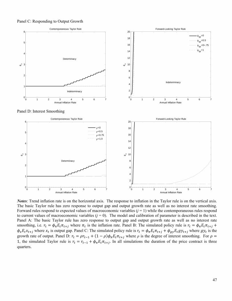
47  

Panel C: Responding to Output Growth

Panel D: Interest Smoothing

Notes: Trend inflation rate is on the horizontal axis. The response to inflation in the Taylor rule is on the vertical axis. The basic Taylor rule has zero response to output gap and output growth rate as well as no interest rate smoothing. Forward rules respond to expected values of macroeconomic variables (j = 1) while the contemporaneous rules respond to current values of macroeconomic variables (j = 0). The model and calibration of parameter is described in the text. Panel A: The basic Taylor rule has zero response to output gap and output growth rate as well as no interest rate smoothing, i.e. where is the inflation rate. Panel B: The simulated policy rule is

where is output gap. Panel C: The simulated policy rule is where is the growth rate of output. Panel D: 1 where ρ is the degree of interest smoothing. For 1, the simulated Taylor rule is . In all simulations the duration of the price contract is three quarters.

0 1 2 3 4 5 6 70

1

2

3

4

5

6Contemporaneous Taylor Rule

Annual Inflation Rate

0 1 2 3 4 5 6 70

2

4

6

8

10

12

14

16

18

20Forward-Looking Taylor Rule

Annual Inflation Rate

gy=0

gy=0.5

gy=0=.75

gy=1

Indeterminacy

Determinacy

Indeterminacy

0 1 2 3 4 5 6 70

1

2

3

4

5

6Contemporaneous Taylor Rule

Annual Inflation Rate

0 1 2 3 4 5 6 70

2

4

6

8

10

12

14

16

18

20Forward-Looking Taylor Rule

Annual Inflation Rate

=0

=0.5

=0.75

=1.0

Determinacy

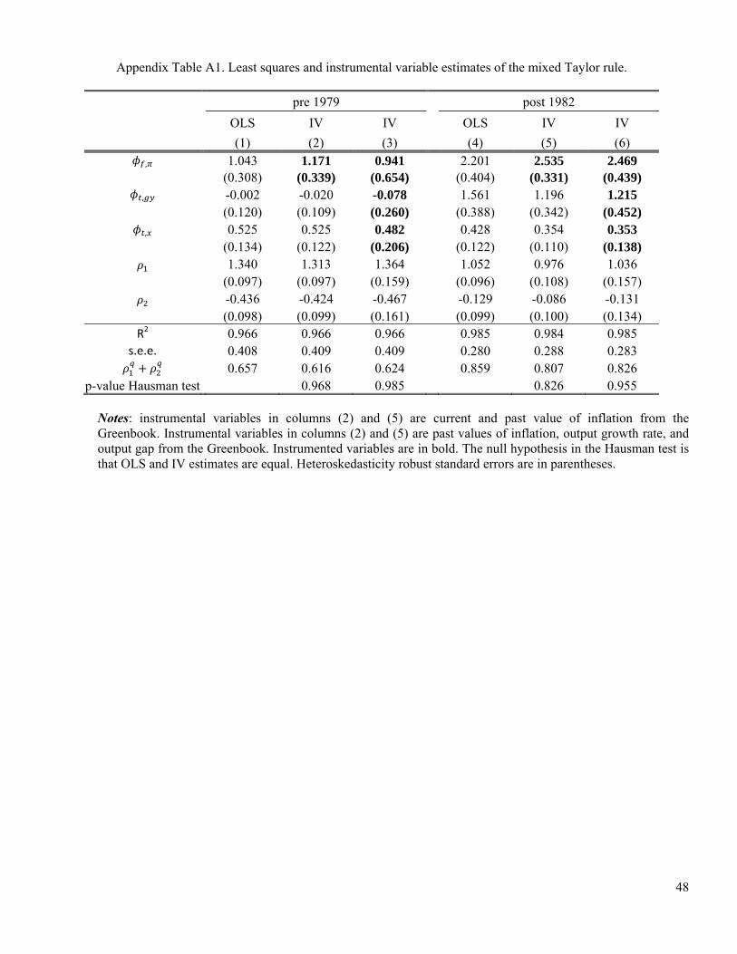
48  

Appendix Table A1. Least squares and instrumental variable estimates of the mixed Taylor rule.

pre 1979 post 1982

OLS IV IV OLS IV IV

      (1) (2) (3) (4) (5) (6)

, 1.043 1.171 0.941 2.201 2.535 2.469(0.308) (0.339) (0.654) (0.404) (0.331) (0.439)

, -0.002 -0.020 -0.078 1.561 1.196 1.215 (0.120) (0.109) (0.260) (0.388) (0.342) (0.452)

, 0.525 0.525 0.482 0.428 0.354 0.353 (0.134) (0.122) (0.206) (0.122) (0.110) (0.138)

1.340 1.313 1.364 1.052 0.976 1.036 (0.097) (0.097) (0.159) (0.096) (0.108) (0.157)

-0.436 -0.424 -0.467 -0.129 -0.086 -0.131 (0.098) (0.099) (0.161) (0.099) (0.100) (0.134)

R2  0.966 0.966 0.966 0.985 0.984 0.985 s.e.e.  0.408 0.409 0.409 0.280 0.288 0.283

  0.657 0.616 0.624 0.859 0.807 0.826 p-value Hausman test 0.968 0.985 0.826 0.955

Notes: instrumental variables in columns (2) and (5) are current and past value of inflation from the Greenbook. Instrumental variables in columns (2) and (5) are past values of inflation, output growth rate, and output gap from the Greenbook. Instrumented variables are in bold. The null hypothesis in the Hausman test is that OLS and IV estimates are equal. Heteroskedasticity robust standard errors are in parentheses.   

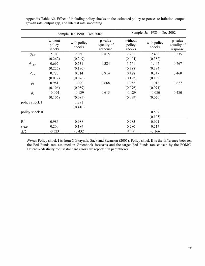
49  

Appendix Table A2. Effect of including policy shocks on the estimated policy responses to inflation, output growth rate, output gap, and interest rate smoothing.

Sample: Jan 1990 – Dec 2002 Sample: Jan 1983 – Dec 2002

without policy shocks

with policy

shocks

p-value equality of response

without policy shocks

with policy

shocks

p-value equality of response

, 2.109 2.050 0.815 2.201 2.438 0.535(0.262) (0.249) (0.404) (0.382)

, 0.697 0.531 0.384 1.561 1.447 0.767 (0.225) (0.190) (0.388) (0.384)

, 0.723 0.714 0.914 0.428 0.347 0.460 (0.077) (0.076) (0.122) (0.109)

0.981 1.020 0.668 1.052 1.018 0.627 (0.106) (0.089) (0.096) (0.071)

-0.094 -0.139 0.615 -0.129 -0.080 0.480 (0.106) (0.089) (0.099) (0.070)

policy shock I 1.271

(0.410)

policy shock II 0.809 (0.105)

R2 0.986 0.988 0.985 0.991 s.e.e. 0.200 0.189 0.280 0.217

AIC -0.323 -0.432 0.326 -0.166

Notes: Policy shock I is from Gürkaynak, Sack and Swanson (2005). Policy shock II is the difference between the Fed Funds rate assumed in Greenbook forecasts and the target Fed Funds rate chosen by the FOMC. Heteroskedasticity robust standard errors are reported in parentheses.

 

 

50  

Appendix Table A3. Model selection

Specification Inflation Output

growth rate Output gap AIC SIC

Log Likelihood

1 Contemp. Contemp. Contemp. 0.737 0.893 -91.31 2 Forecast Forecast Forecast 0.808 0.965 -100.86 3 Contemp. Contemp. Forecast 0.735 0.891 -91.18 4 Contemp. Forecast Contemp. 0.822 0.979 -102.14 5 Contemp. Forecast Forecast 0.830 0.987 -103.32 6 (baseline) Forecast Contemp. Contemp. 0.723 0.880 -88.72 7 Forecast Forecast Contemp. 0.794 0.951 -98.92 8 Forecast Contemp. Forecast 0.724 0.881 -89.09

Notes: the table reports information criteria and log-likelihood for Taylor rules with the baseline and alternative choices of current vs. forecast values of inflation, output growth rate and output gap.

Appendix Table A4. Forecast horizon in the policy reaction function and the determinacy rates.

pre 1979 policy rule post 1982 policy rule

3% trend inflation

6% trend inflation

3% trend inflation

6% trend inflation

Horizon

t+1 7.9% 0.0% 99.2% 61.0%

t+2 5.2% 0.0% 99.3% 61.1%

t+3 1.9% 0.0% 98.9% 60.9%

t+4 0.5% 0.0% 97.2% 59.4%

Average inflation rate a given horizon

t+1,t+2 (baseline) 7.5% 0.0% 99.4% 62.2%

t+1 through t+3 5.7% 0.0% 99.2% 62.0%

t+1 through t+4 3.4% 0.0% 99.1% 61.9% Notes: The policy reaction function uses estimated coefficients and associated covariance matrix for the mixed Taylor rule reported in Table 1.

51  

Appendix A: Proof of Proposition 1.

Woodford (2003, Proposition 6.1) considers second order approximation of t

ttE U (A.1)

where per period utility is given by 1 1

0 0

( ) ( ( )) ( ) ( ( ))t t t t tU u C N i di u C Y i di . We consider a modified utility

1

1

0

( ) ( ) ( ( ))t t t tU u C hu C Y i di

where h is the degree of habit formation in consumption. First, we do the expansion of the utility derived from consumption around flexible price steady state

1

1 1

1 1

211 1 12

211 12

2 2 21 112 2

( ) ( ) ( ) ( )

( ) ( ) ( ) ( ) ( )

( )

ˆ ˆ ˆ( ) ( )

F F F Ft t t t

F Ft t

F F Ft t t t

t t t t

F F F F Ft t t t t t t tY Y Y Y

tip

Ft tY Y

F F Ft t t t t tY Y Y Y

u C hu C u Y hu Y

u Y hu Y u Y Y u Y Y hu Y Y

hu Y Y hot

Y u X X Y u Y hY u

1

1 1

1

1 1 1

1

211 2

2 211 12

2 211 1 2

2 211 1 12

1

ˆ ˆ( )

ˆ( )

ˆ ˆ ˆ( ( ) )

ˆ( ( ) )

ˆ

F

F Ft t

F F F F Ft t t t t

F F Ft t t

F Ft t

t t

Ft tY Y

F F F Ft t t t t t tY Y Y Y Y

F Ft t tY Y Y

F Ft t tY Y

X X

h Y u X hot tip

Y u X hY u X Y u u Y X

h Y u u Y X hot tip

Y u X hY u

11 1

11

211 2

211 12

ˆ ˆ(1 )

ˆ(1 )

FF F tY Yt t

FFt Yt

FF F tY Yt t

FFt Yt

u YF

t t tuY

u YF

t tuY

X Y u X

hY u X hot tip

11

1

1 2 1 21 11 1 12 2

ˆ ˆ ˆ ˆ( ) (1 ) (1 )F

t FYtF F FF

t t tt FYt

Y uF

t t t t t t tY Y YY uY u X h X Y u X hY u X hot tip

(A.2)

where is the intertemporal elasticity of substitution for consumption, is the elasticity of real marginal cost with

respect to own output, FtY is the flexible price level of output at time t, hats denote percent deviations, tip stands for

terms independent from policy, hot means higher order terms.

Given assumption about log utility in consumption, we have 1(1 ) 0 and all second order terms drop.

Furthermore, from the same assumption we have 1

1( ) / ( ) 1F Ft t

F Ft tY Y

Y u Y u

and 1Ft

Ft Y

Y u . Hence,

1 1ˆ ˆ( ) ( )t t t tu C hu C X hX hot tip . (A.3)

Now consider the expansion of the utility part that corresponds to disutility from labor supply.

212

ˆ ˆ( ( )) ( ) (1 ) ( )Ft

Ft t t tY

y i di Y y i y i tip (A.4)

where ˆ ( ) log( ( ) / )Ft t ty i y i Y is the deviation of firm i’s output from flexible price level of output F

tY . Compute the

average across firms 1 1

212

0 0

ˆ ˆ( ( )) ( ) (1 ) ( )Ft

Ft t i t tY

Y i di Y E y i y i di hot

(A.5)

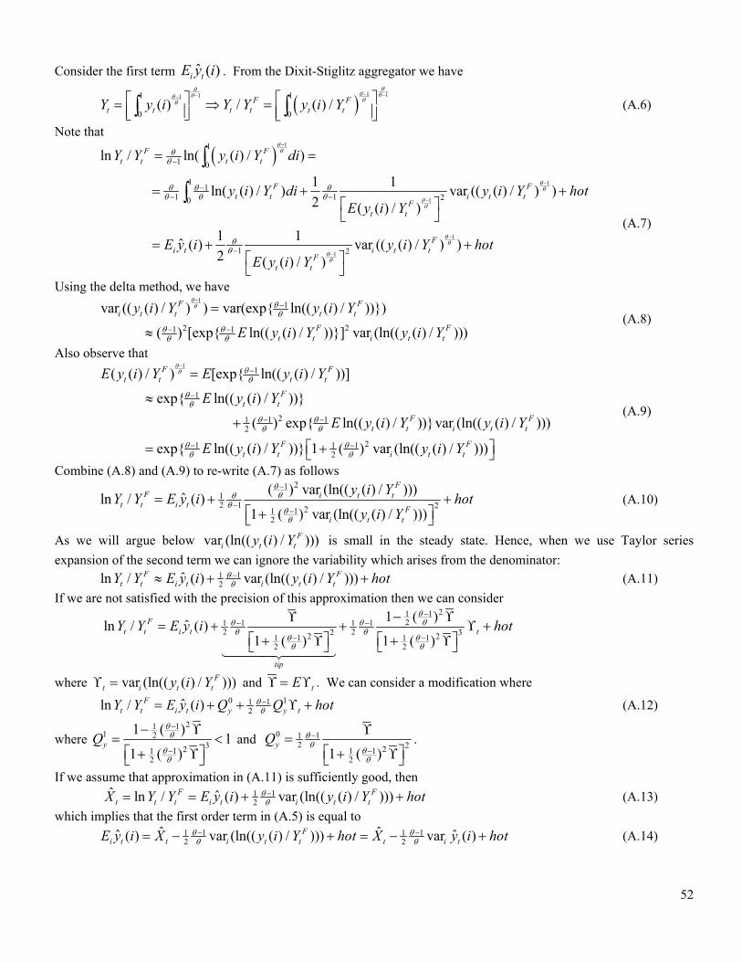
52  

Consider the first term ˆ ( )i tE y i . From the Dixit-Stiglitz aggregator we have

1 1111 1

0 0( ) / ( ) /F F

t t t t t tY y i Y Y y i Y

(A.6)

Note that

1

1

1

1

1

1

1 0

11

1 1 20

1 2

ln / ln( ( ) / )

1 1ln( ( ) / ) var (( ( ) / ) )

2 ( ( ) / )

1 1ˆ ( ) var (( ( ) / ) )

2 ( ( ) / )

F Ft t t t

F Ft t i t t

Ft t

Fi t i t t

Ft t

Y Y y i Y di

y i Y di y i Y hotE y i Y

E y i y i Y hotE y i Y

(A.7)

Using the delta method, we have 1

1

2 21 1

var (( ( ) / ) ) var(exp{ ln(( ( ) / ))})

( ) [exp{ ln(( ( ) / ))}] var (ln(( ( ) / )))

F Fi t t t t

F Ft t i t t

y i Y y i Y

E y i Y y i Y

(A.8)

Also observe that 1

1

1

21 112

21 112

( ( ) / ) [exp{ ln(( ( ) / ))]

exp{ ln(( ( ) / ))}

( ) exp{ ln(( ( ) / ))}var (ln(( ( ) / )))

exp{ ln(( ( ) / ))} 1 ( ) var (ln(( ( ) / )))

F Ft t t t

Ft t

F Ft t i t t

F Ft t i t t

E y i Y E y i Y

E y i Y

E y i Y y i Y

E y i Y y i Y

(A.9)

Combine (A.8) and (A.9) to re-write (A.7) as follows 21

12 1 2211

2

( ) var (ln(( ( ) / )))ˆln / ( )

1 ( ) var (ln(( ( ) / )))

FF i t t

t t i tF

i t t

y i YY Y E y i hot

y i Y

(A.10)

As we will argue below var (ln(( ( ) / )))Fi t ty i Y is small in the steady state. Hence, when we use Taylor series

expansion of the second term we can ignore the variability which arises from the denominator: 11

2ˆln / ( ) var (ln(( ( ) / )))F F

t t i t i t tY Y E y i y i Y hot (A.11)

If we are not satisfied with the precision of this approximation then we can consider

211

21 11 12 22 32 21 11 1

2 2

1 ( )ˆln / ( )

1 ( ) 1 ( )

Ft t i t t

tip

Y Y E y i hot

where var (ln(( ( ) / )))Ft i t ty i Y and tE . We can consider a modification where

0 1112

ˆln / ( )Ft t i t y y tY Y E y i Q Q hot

(A.12)

where 211

1 23211

2

1 ( )1

1 ( )yQ

and 0 112 2211

21 ( )yQ

.

If we assume that approximation in (A.11) is sufficiently good, then

112

ˆ ˆln / ( ) var (ln(( ( ) / )))F Ft t t i t i t tX Y Y E y i y i Y hot

(A.13)

which implies that the first order term in (A.5) is equal to 1 11 1

2 2ˆ ˆˆ ˆ( ) var (ln(( ( ) / ))) var ( )F

i t t i t t t i tE y i X y i Y hot X y i hot (A.14)

53  

Now consider the second term in (A.5): 1 1

2 2 2

0 0

ˆ ˆ ˆ ˆ ˆ ˆ( ) [ ( ) ( ) ( )] var ( ) [ ( )]t t i t i t i t i ty i di y i E y i E y i di y i E y i (A.15)

Using (A.14), we can re-write (A.15) as follows 1

2 2112

0

2 2 21 114

2

ˆˆ ˆ ˆ( ) var ( ) [ var ( )]

ˆ ˆˆ ˆ ˆvar ( ) ( ) [var ( )] var ( )

ˆˆvar ( )

t i t t i t

i t t i t t i t

hot

i t t

y i di y i X y i

y i X y i X y i

y i X hot

(A.16)

If approximation in (A.11) is not satisfactory, then (A.16) would be 1

2 0 1 2112

0

2 2 1 2 1 0 2 0 0 11 1 114

0 11

ˆˆ ˆ ˆ( ) var ( ) [ var ( )]

ˆ ˆ ˆˆ ˆ ˆ ˆvar ( ) ( ) [ var ( )] var ( ) [ ] 2 var ( )

(1 ) var

t i t t y y i t

i t t y i t t y i t y y t y y i t

hot tip

y y i

y i di y i X Q Q y i

y i X Q y i X Q y i Q Q X Q Q y i

Q Q

2 0ˆ ˆˆ ( ) 2t t y ty i X Q X hot tip Now we combine (A.16) and (A.14) to finally get the part which corresponds to the second-order approximation of utility due to the disutility of labor supply (A.5):

1 121

20 0

211 12 2

1 21 12 2

ˆ ˆ( ( )) ( ) (1 ) ( )

ˆ ˆˆ ˆvar ( ) (1 )(var ( ) )

ˆ ˆˆ( ) var ( ) (1 ) )

Ft

Ft

Ft

Ft t i t tY

Ft t i t i t tY

Ft t i t tY

Y i di Y E y i y i di hot

Y X y i y i X hot tip

Y X y i X hot tip

(A.17)

Again, if we are not satisfied with the quality of approximation in (A.11), then (A.17) will be

1 121

20 0

1 0 1 2 01 11 12 2

0 1 1 112

ˆ ˆ( ( )) ( ) (1 ) ( )

ˆ ˆ ˆˆ ˆvar ( ) (1 )([1 ]var ( ) 2 )

ˆ(1 (1 ) ) ( (1 )(1

Ft

Ft

Ft

Ft t i t tY

Ft t y i t y y i t t y tY

Ft y t y yY

Y i di Y E y i y i di hot

Y X Q y i Q Q y i X Q X hot tip

Y Q X Q Q

0 1 21 12

ˆˆ)) var ( ) (1 ) )y y i t tQ Q y i X hot tip

As Woodford (2003) shows, (1 ) (1 )F F

t tY Yh u which follows from the intra-temporal condition for labor

supply. He also argues that the (1 ) multiplier can be ignored on terms other the first term in (A.17) so that

1

1 21 12 2

0

ˆ ˆˆ( ( )) (1 ) (1 ) ( ) var ( ) (1 ) )Ft

Ft t t i t tY

Y i di h Y u X y i X hot tip (A.18)

We now want to evaluate ˆvar ( )i ty i in (A.18). To replace variability of output with variability of prices we will use

ˆ ( ) ln ( ) ln ln ln {ln ( ) ln }F Ft t t t t t ty i y i Y Y Y p i P (A.19)

Since ln ln Ft tY Y and ln tP are the same across firms, we have

2ˆvar ( ) var ln ( )i t i ty i p i (A.20)

54  

Define ln( / )t t tb B P (note that in our notation bt is the price relative to current price level) and log ( )t i tP E p i ,

and 1/(1 )1 1

0( ) .t tP p i di

1 1 12 2 2

0 0 1

1 1 12 2

0 0 0

1

var (ln ( )) [ln ( ) ] [ln ( ) ] [ln ( ) ]

[ln ( ) ln ] 2 [ln ( ) ln ][ln ] [ln ]

[ln ( )

t i t t t t t t t

pricechange fixed price

t t t t t t t t

t

p i p i P di p i P di p i P di

p i P di p i P P P di P P di

p i

1 1 12 2

1 1 1 1 1

1 1 1

] 2 [ln ( ) ][ ] [ ]t t t t t t tP di p i P P P di P P di

2 2

12

1 1 1 1 1

1

0

(1 ) 2(1 ) [ln ] (1 )[ln ]

2[ ] [ln ( ) ] [ ]

t t t t t t

t t t t t t t

b b P P P P

P P p i P di P P

So that 2 2 2

1 1(1 ) 2(1 ) [ln ] (1 )[ln ] [ ]t t t t t t t t t tb b P P P P P P (A.21)

We start with the term ln t tP P . Note

1 11 1 120 0 1

1 1 1 1 1ln ln( ( ) ) ln( ( )) var ( ( ))

1 1 2 1 ( )t

t t t i t

tP

P p i di p i di p i hotEp i

(A.22)

From the delta method, we have 1 2 2

2 2

2 2

var ( ( )) var (exp{(1 ) ln ( )}) (1 ) [exp{(1 ) ln ( )}] var (ln ( ))

(1 ) [exp{(1 ) }] var (ln ( ))

(1 ) [exp{(1 ) }]

i t i t t i t

t i t

t t

p i p i E p i p i

P p i

P

(A.23)

Now observe that 1

212

2 21 12 2

( ) [exp{(1 ) ln ( )}] exp{(1 ) ln ( )}

(1 ) exp{(1 ) ln ( )}var (ln ( ))

exp{(1 ) } (1 ) exp{(1 ) } exp{(1 ) }[1 (1 ) ]

t

t t t

t i t

t t t t t

Ep i E p i E p i

E p i p i

P P P

(A.24)

Hence it follows that 2 2

22 212

2212

212

2 32 21 12 2

(1 ) [exp{(1 ) }]1 1ln

2 1 [exp{(1 ) }] 1 (1 )

(1 )1

2 1 (1 )

1 (1 )1 1

2 21 (1 ) 1 (1 )

t tt t

t t

tt

t

t t

PP P hot

P

P hot

P hot

(A.25)

where (var ln ( ))t i tE E p i is the dispersion of prices in the steady state. In the zero trend inflation

approximation, 0 . With positive trend inflation, is small (see below). So if close to zero, then

55  

212

2 22 21 12 2

0 1

1 (1 )1 1ln

2 21 (1 ) 1 (1 )

1

2

t t t

t t

P P hot

P hot

(A.26)

If we are not satisfied with the quality of the approximation, we can consider 0 11

2ln t t p p tP P Q Q hot (A.27)

where 0221

2

1

2 1 (1 )pQ

and

211 2

2212

1 (1 )

1 (1 )pQ

which is close to one. Hence,

0 112ln t t p p tP P Q Q hot (A.28)

If we take the approximation as reasonably accurate, we then have 1 1

2 2ln lnt t t t t tP P hot P P (A.29)

Also from our derivations in the paper we have that 1 1

01 1

1

1t t t t tb b M

. (A.30)

Plug (A.30) and (A.29) into (A.21) to get 2(1 )2 2 2

14

21 1 1

2 2 21 1

2 21 1

1

(1 ) (1 )(1 ) (1 )

[(ln ln ) (ln ) (ln )]

(1 ) [ln ln ]

[ln ] [ln ]

2 [ln ln ][ln

t t t t t t

hot hot

t t t t t t

t t t t

t t t t

t t t

M M

P P P P P P

M P P

P P P P

P P P P

2 2

1 1 1

1 1

2 2 21

(1 ) (1 )2 2 21 1 14 4

2 2

] 2 [ln ln ][ln ]

2 [ln ][ln ]

(1 )

(1 ) (1 ) 2 (1 )

[(1 ) ]

t t t t t

t t t t

t t t

t t t t t t t t

hot

t

P P P P

P P P P hot

M

hot

M

1t hot

(A.31)

So the only difference in the end is that 1

11M

instead of

1M

.

If we want to use a more precise expression for the ln t tP P such as (A.28), we would have

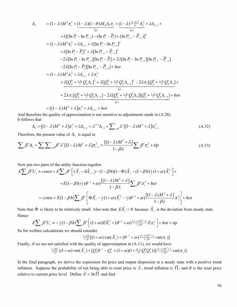
56  

2(1 )2 2 20 14

21 1 1

2 2 21 1

2 21 1

1

(1 ) (1 )(1 ) (1 )

[(ln ln ) (ln ) (ln )]

(1 ) [ln ln ]

[ln ] [ln ]

2 [ln ln ][ln

t t t t t t

hot hot

t t t t t t

t t t t

t t t t

t t t

M M

P P P P P P

M P P

P P P P

P P P

1 1 1

1 1

2 2 21

0 1 2 0 1 2 0 11 1 112 2 2

0 1 0112

] 2 [ln ln ][ln ]

2 [ln ][ln ]

(1 )

[ ] [ ] 2 [ ]

2 [ ] 2 [

t t t t t

t t t t

t t t

p p t p p t t p p t

hot

t p p t p

P P P P P

P P P P hot

M

Q Q Q Q Q Q

Q Q Q

1 0 11 112 2

2 21

][ ]

[(1 ) ]

p t p p t

hot

t t

Q Q Q hot

M hot

And therefore the quality of approximation is not sensitive to adjustments made in (A.28). It follows that

2 2 1 2 21 1 0

[(1 ) ] [(1 ) ]tt s

t t t t ssM M

(A.32)

Therefore, the present value of t is equal to 2

2 2 2

0

[(1 ) ][(1 ) ]

1

tt t s tt t s tt t s t

MM tip

(A.33)

Now put two parts of the utility function together

211 2

21 21

2

22 1 21 1

2 2

ˆ ˆ ˆ ˆ( ) (1 )(1 ) (1 ) (1 )

[(1 ) ](1 ) ( )

1

[(1 ) ]ˆ ˆ(1 ) (1 ) ( )1

t tt t t t tt t

ttt

tt t tt

E U const E X hX h X h X

ME h hot

Mconst E h X X hot

Note that is likely to be relatively small. Also note that ˆ 0tEX because ˆtX is the deviation from steady state.

Hence 2(1 )2 1 21

2 1ˆ(1 ) (1 ) ( ) Mt t

t t tt tE U h EX E hot tip

So for welfare calculations we should consider 2(1 )1 1

1 1ˆ[(1 ) var( ) ( ) var( )]Mh

t tX

Finally, if we are not satisfied with the quality of approximation in (A.11), we would have 2(1 )1 1 1 1 0 11

1 1ˆ{(1 ) var( ) [ (1 )(1 ))] var( )}Mh

t y y y y tX Q Q Q Q

In the final paragraph, we derive the expression for price and output dispersion in a steady state with a positive trend

inflation. Suppose the probability of not being able to reset price is , trend inflation is , and B is the reset price

relative to current price level. Define ln and find

57  

2

0 0 0

10 (1 )

ln ( ) (1 ) ln( / ) (1 ) ln( ) (1 )

ln( ) (1 ) ln( ) (1 ) ln( )

s s s st t s s s

s

s

E p i P B B s

B s B B

 

2

2

2

2

2

2 2

2 210 0

2 2 2 210 0 0(1 )

2 2 2 2

0 0(1 )

(12 2 2

(1 ) (1 )

var ln ( ) (1 ) [ln( / ) ] (1 ) [ ]

(1 ) 2 (1 ) (1 )

2 (1 )

2 (1 )

s s si t ts s

s s s

s s s

s s

s s

E p i B P s

s s

s s

3

2

2

)

(1 )

2

(1 )

2

(1 )

[ 2 (1 )]

 

Since is small for inflation up to 20%, var ln ( ) 0i tE p i . Also note that 2ˆvar ( ) var ln ( )i t i tE y i E p i and

hence if var ln ( ) 0i tE p i , then ˆvar ( ) 0i tE y i . For example at 1.06 annually and our baseline

calibration, ˆvar ( ) 0.05i tE y i .