monetarypolicyandthefirm: someempiricalevidence1 · share of total jobs (%) ... url....

Monetary Policy and the Firm: Some Empirical Evidence1

Saleem Bahaj Angus Foulis Gabor Pinter

Bank of England

9 October 2017

1The views expressed are those of the presenter and not necessarily those of the Bank ofEngland, the MPC, the FPC or PRA Board.

Bahaj-Foulis-Pinter (Bank of England) Monetary Policy and the Firm 10/2017

What We Do in this Paper

How does the individual firm respond to a monetary policy shock?how does the response compare to aggregate dynamics?how do firm characteristics govern the extent of this response?

Focusing on size and age

In this paper we:answer these questions with microdata on a panel of UK firms covering1990-2015.monetary policy shocks identified using high frequency market surprises(Miranda-Agrippino [2016]).


What We Find

Monetary policy has a much more persistent effect on incumbent firmsaggregate economy returns to normal after 5 years;after 5 years firm response is hitting its peak.

New entrants can reconcile this.With delay, monetary policy increases size at entry.And, eventually, rates of entry.

Who is most affected by policy?Large firms more than small firms & young firms more than old.Young, large firms the most.

monetary policy redistributes activity from recent (large) entrants to futureentrants (by making them bigger).Work in progress.

Cleansing vs scarring (Caballero and Hammour [1994], Ouyang [2009]).What mechanism explains the persistence?


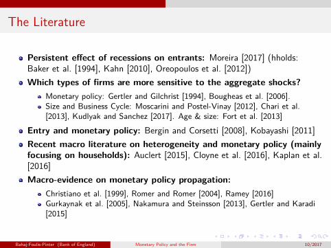
The Literature

Persistent effect of recessions on entrants: Moreira [2017] (hholds:Baker et al. [1994], Kahn [2010], Oreopoulos et al. [2012])Which types of firms are more sensitive to the aggregate shocks?

Monetary policy: Gertler and Gilchrist [1994], Bougheas et al. [2006].Size and Business Cycle: Moscarini and Postel-Vinay [2012], Chari et al.[2013], Kudlyak and Sanchez [2017]. Age & size: Fort et al. [2013]

Entry and monetary policy: Bergin and Corsetti [2008], Kobayashi [2011]Recent macro literature on heterogeneity and monetary policy (mainlyfocusing on households): Auclert [2015], Cloyne et al. [2016], Kaplan et al.[2016]Macro-evidence on monetary policy propagation:

Christiano et al. [1999], Romer and Romer [2004], Ramey [2016]Gurkaynak et al. [2005], Nakamura and Steinsson [2013], Gertler and Karadi[2015]


Firm DataOverview

Accounting Data: Bureau van Dijk (BVD) based on filings at Companies House(UK registrar)

Annual data covering ~4.0 million UK firms annual company house filings.

BVD is a live database, which leads to several limitations, most importantly:selection issue, firms that die leave the database after ~ 5years.

Illustrating the Selection Effect

To circumvent this issue, we use archived data sampled at a six monthlyfrequency to capture information when it was first published.


DataTreatment of Firms

Sample selection:we exclude companies that have a parent with an ownership stake greater than50%.operate in finance, utilities or public sectors.Firms must be active, have operated for at least three years and reportvariables of interest.

Sample period is 1990-2015 (95% obs in 1998-2014).Annual data but firms have different accounting periods.

Jan, 06

Jun, 06

Jan, 07

Jun, 07

��

��


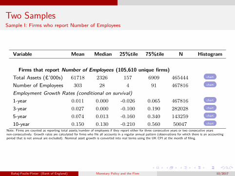
Two SamplesSample I: Firms who report Number of Employees

Variable Mean Median 25%tile 75%tile N Histogram

Firms that report Number of Employees (105,610 unique firms)Total Assets (£’000s) 61718 2326 157 6909 465444 chart

Number of Employees 303 28 4 91 467816 chart

Employment Growth Rates (conditional on survival)1-year 0.011 0.000 -0.026 0.065 467816 chart

3-year 0.027 0.000 -0.100 0.190 282028 chart

5-year 0.074 0.013 -0.160 0.340 143259 chart

10-year 0.150 0.130 -0.210 0.560 50047 chart

Note: Firms are counted as reporting total assets/number of employees if they report either for three consecutive years or two consecutive yearsnon-consecutively. Growth rates are calculated for firms who file all accounts in a regular annual pattern (observations for which there is an accountingperiod that is not annual are excluded). Nominal asset growth is converted into real terms using the UK CPI at the month of filing.


Two SamplesSample II: Firms who report Total Assets

Variable Mean Median 25%tile 75%tile N Histogram

Firms that report Total Assets (3,744,718 unique firms)Total Assets (£’000s) 2779 55 15 225 12050499 chart

Real Asset Growth (conditional on survival)1-year 0.022 0.000 -0.160 0.220 12050499 chart

3-year 0.068 0.031 -0.260 0.430 8072643 chart

5-year 0.160 0.120 -0.310 0.670 4462878 chart

10-year 0.330 0.300 -0.270 0.990 1366788 chart

Note: Firms are counted as reporting total assets/number of employees if they report either for three consecutive years or two consecutive yearsnon-consecutively. Growth rates are calculated for firms who file all accounts in a regular annual pattern (observations for which there is an accountingperiod that is not annual are excluded). Nominal asset growth is converted into real terms using the UK CPI at the month of filing.


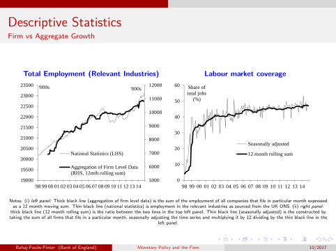
Descriptive StatisticsFirm vs Aggregate Growth

Total Employment (Relevant Industries) Labour market coverage

5000

6000

7000

8000

9000

10000

11000

12000

19000

19500

20000

20500

21000

21500

22000

22500

23000

23500

98 99 00 01 02 03 04 05 06 07 08 09 10 11 12 13 14

'000s'000s

National Statistics (LHS)

Aggregation of Firm Level Data(RHS, 12mth rolling sum)

0

10

20

30

40

50

60

98 99 00 01 02 03 04 05 06 07 08 09 10 11 12 13 14

Share of total jobs

(%)

Seasonally adjusted

12 month rolling sum

Notes: (i) left panel: Thick black line (aggregation of firm level data) is the sum of the employment of all companies that file in particular month expressedas a 12 month moving sum. Thin black line (national statistics) is employment in the relevant industries as sourced from the UK ONS. (ii) right panel:thick black line (12 month rolling sum) is the ratio between the two lines in the top left panel. Thin black line (seasonally adjusted) is the constructed bytaking the sum of all firms that file in a particular month, seasonally adjusting the time series and multiplying it by 12 dividing by the thin black line in the

left panel.


Descriptive StatisticsBirth and Death

Births Deaths

0

50

100

150

200

250

300

98 99 00 01 02 03 04 05 06 07 08 09 10 11 12 13 14

Births, '000s

0

50

100

150

200

250

98 99 00 01 02 03 04 05 06 07 08 09 10 11 12 13 14

Deaths, '000s

Notes: (i) left panel: number of firms with incorporation date in a rolling 12 month window. (ii) right panel: number of firms with a statement date wherethe company status was first listed as dissolved in a rolling 12 month window.


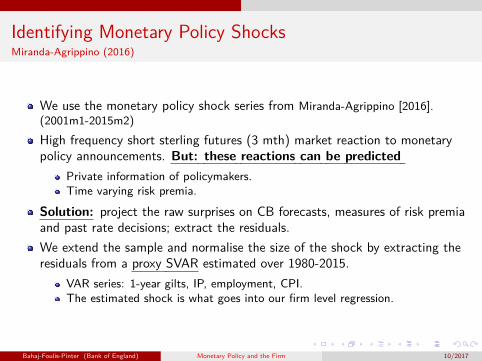
Identifying Monetary Policy ShocksMiranda-Agrippino (2016)

We use the monetary policy shock series from Miranda-Agrippino [2016].(2001m1-2015m2)High frequency short sterling futures (3 mth) market reaction to monetarypolicy announcements. But: these reactions can be predicted

Private information of policymakers.Time varying risk premia.

Solution: project the raw surprises on CB forecasts, measures of risk premiaand past rate decisions; extract the residuals.We extend the sample and normalise the size of the shock by extracting theresiduals from a proxy SVAR estimated over 1980-2015.

VAR series: 1-year gilts, IP, employment, CPI.The estimated shock is what goes into our firm level regression.


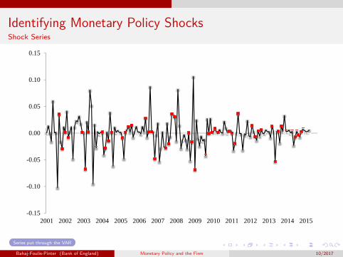
Identifying Monetary Policy ShocksShock Series

-0.15

-0.10

-0.05

0.00

0.05

0.10

0.15

2001 2002 2003 2004 2005 2006 2007 2008 2009 2010 2011 2012 2013 2014 2015

Series put through the VAR


Aggregate Responses1sd monthly contractionary shock

1 Year Yields Employment

Notes: Estimates are from a proxy SVAR estimated on UK monthly data over the period 1981-2015. Monetarypolicy shocks are identified using the Miranda-Agrippino [2016] series. The blue solid lines are the point

estimates, and the shaded areas are the 90% confidence intervals constructed from a wild recursive bootstrap.

Output and Prices


Empirical Methodology

Specification:

log(EMPt+h,i )− log(EMPt−1,i ) = αhi +β

h12∑

m=1

wmem,t +γh ×controlsi,t +

4∑j=1

φh12∑

m=1

um,j,t +εhi,t

t is an index of time denoting firm account years (we ignore observationswhere firms have irregular filing periods).m denotes months over a firm’s account year =>

∑12m=1 wmem,t is the

weighted sum of monetary shocks over the accounting year.We show wm = 1, results robust to other weights.

Inference:multiway clustering to account for overlapping time windows.plus cluster at the industry level.


Employment Responses: 1sd annual contractionary shock

-7

-6

-5

-4

-3

-2

-1

0

1

0 1 2 3 4 5 6 7 8 9 10

Cumulative % Chg

Years since shock

Notes: Firm level responses to a 1 standard deviation contractionary monetary policy shock. Black dotted lines are point estimates. Grey shaded areas are90% confidence intervals constructed from a tG−1 distribution where G is the minimum of clusters in the regression. The dependent variable is the

cumulative growth rate in log points of employment from t − 1 to t + h where t is the date of the monetary policy shock and h is the x-axis. Sample is105,610 unique UK firms over the period 1990-2015 (at h = 0 zero this corresponds to 467,816 firm-year observations).


Employment Responses: 1sd annual contractionary shock

-7

-6

-5

-4

-3

-2

-1

0

1

0 1 2 3 4 5 6 7 8 9 10

Cumulative % Chg

Years since shockAggregate Response




Total Asset Responses: 1sd annual contractionary shock

-24

-20

-16

-12

-8

-4

0

4

0 1 2 3 4 5 6 7 8 9 10

Cumulative % Chg

Years since shock




Robustness

Alternative Estimators

Alternative Specifications

Alternative Instruments

Monte Carlo Study


Reconciling the evidence

Births Size at Birth

Notes: Aggregate responses to a 1 standard deviation monthly monetary policy shock. Local projectionsestimated using UK monthly data 1998-2014. Blue solid line is the point estimate, shaded areas are 90%

confidence intervals constructed from a HAC adjusted standard errors. Left panel: log change in incorporationsof new enterprises from t − 1 to t + h where t is the date of the monetary policy shock. Right panel: average

birth size measured as real total assets.


Which incumbents repond?

If new entrants generate the recovery, useful to ask which incumbents aremost sensitive in the first place.Subject of debate:

Small versus large firms. Gertler and Gilchrist [1994],Moscarini andPostel-Vinay, 2012, Chari et al., 2013, Kudlyak and Sanchez, 2017.Young versus old firms. Fort et al. [2013]

First condition on quintiles of the age and size distribution.Then do the double sort.

Quintile Values


The effect of age

Number of Employees Total Assets

-12

-10

-8

-6

-4

-2

0

2

0 1 2 3 4 5 6 7 8 9 10

Cumulative % Chg

Years since shock

��

��

��

��

��

-25

-20

-15

-10

-5

0

5

0 1 2 3 4 5 6 7 8 9 10

Cumulative % Chg

Years since shock

��

��

��

��

Notes: Firm level responses to a 1 standard deviation contractionary monetary policy shock. point estimates for response for firms in the five differentportions of the age distribution (when the shock hit).

oldest vs youngest quintiles


The effect of size


-12

-10

-8

-6

-4

-2

0

2

0 1 2 3 4 5 6 7 8 9 10

Cumulative % Chg

Years since shock

��

��

��

��

��

-20

-15

-10

-5

0

5

10

0 1 2 3 4 5 6 7 8 9 10

Cumulative % Chg

Years since shock

��

��

��

��

��

Notes: Firm level responses to a 1 standard deviation contractionary monetary policy shock.Point estimates for response for firms in the five differentportions of the size distribution (when the shock hit).

smallest vs largest quintiles


Double Sort: Size and Age I

Small, Young firms Small, Old firms

-10

-8

-6

-4

-2

0

2

4

6

8

10

0 1 2 3 4 5 6 7 8 9 10

Effect of 1sd chg on

Cum. % Chg

Years since shock-10

-8

-6

-4

-2

0

2

4

6

8

10

0 1 2 3 4 5 6 7 8 9 10


Cum. % Chg

Years since shock

Notes: Firm level responses to a 1 standard deviation contractionary monetary policy shock. The dependent variable is the cumulative growth rate in logpoints of employment from t − 1 to t + h where t is the date of the monetary policy shock and h is the x-axis. Black dotted lines are point estimates.

Grey dash lines enclose 90% confidence intervals constructed from a tG−1 distribution where G is the minimum of clusters in the regression. Small = firmin first two quintiles of the size distribution (measured by assets) when the shock hits. Young = firm in first two quintiles of the age distribution when the

shock hits. Large = firm in fifth quintile of the size distribution (measured by assets) when the shock hits. Old = firm in the fifth quintile of the agedistribution when the shock hits.

frequency table


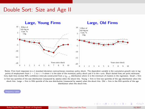
Double Sort: Size and Age II

Large, Young Firms Large, Old Firms

-20

-15

-10

-5

0

5

10

0 1 2 3 4 5 6 7 8 9 10


Cum. % Chg

Years since shock-20

-15

-10

-5

0

5

10

0 1 2 3 4 5 6 7 8 9 10


Cum. % Chg

Years since shock

Notes: Firm level responses to a 1 standard deviation contractionary monetary policy shock. The dependent variable is the cumulative growth rate in logpoints of employment from t − 1 to t + h where t is the date of the monetary policy shock and h is the x-axis. Black dotted lines are point estimates.

Grey dash lines enclose 90% confidence intervals constructed from a tG−1 distribution where G is the minimum of clusters in the regression. Small = firmin first two quintiles of the size distribution (measured by assets) when the shock hits. Young = firm in first two quintiles of the age distribution when the

shock hits. Large = firm in fifth quintile of the size distribution (measured by assets) when the shock hits. Old = firm in the fifth quintile of the agedistribution when the shock hits.

frequency table


Conclusions

Provided novel empirical evidence on the impact of monetary policy shocks.Monetary policy has far more persistent effects on individual firms than onthe aggregate.Behaviour of entrants can reconcile this.Large, new entrants more vulnerable.


ReferencesAdrien Auclert. Monetary policy and the redistribution channel. 2015 Meeting Papers

381, Society for Economic Dynamics, 2015. URLhttp://EconPapers.repec.org/RePEc:red:sed015:381.

George Baker, Michael Gibbs, and Bengt Holmstrom. The wage policy of a firm. TheQuarterly Journal of Economics, 109(4):921–955, 1994.

Paul R. Bergin and Giancarlo Corsetti. The extensive margin and monetary policy.Journal of Monetary Economics, 55(7):1222–1237, October 2008. URLhttps://ideas.repec.org/a/eee/moneco/v55y2008i7p1222-1237.html.

Spiros Bougheas, Paul Mizen, and Cihan Yalcin. Access to external finance: Theory andevidence on the impact of monetary policy and firm-specific characteristics. Journal ofBanking & Finance, 30(1):199 – 227, 2006. ISSN 0378-4266. doi:http://doi.org/10.1016/j.jbankfin.2005.01.002. URLhttp://www.sciencedirect.com/science/article/pii/S0378426605000312.

Ricardo J Caballero and Mohamad L Hammour. The cleansing effect of recessions.American Economic Review, 84(5):1350–1368, December 1994. URLhttps://ideas.repec.org/a/aea/aecrev/v84y1994i5p1350-68.html.

Ambrogio Cesa-Bianchi, Gregory Thwaites, and Alejandro Vicondoa. Monetary policytransmission in an open economy: New data and evidence from the united kingdom.Discussion Papers 1612, Centre for Macroeconomics (CFM), April 2016. URLhttps://ideas.repec.org/p/cfm/wpaper/1612.html.

V. V. Chari, Lawrence J. Christiano, and Patrick J. Kehoe. The gertler-gilchrist evidenceon small and large firm sales. mimeo, Northwestern University, 2013.

Lawrence J. Christiano, Martin Eichenbaum, and Charles L. Evans. Monetary policyshocks: What have we learned and to what end? In J. B. Taylor and M. Woodford,editors, Handbook of Macroeconomics, volume 1, chapter 2, pages 65–148. Elsevier,1999. URL https://ideas.repec.org/h/eee/macchp/1-02.html.

James Cloyne and Patrick Hurtgen. The macroeconomic effects of monetary policy: anew measure for the united kingdom. American Economic Journal: Macroeconomics,8(4):75–102, October 2016.

James Cloyne, Clodomiro Ferreira, and Paolo Surico. Monetary policy when householdshave debt: new evidence on the transmission mechanism. Bank of England workingpapers 589, Bank of England, April 2016. URLhttps://ideas.repec.org/p/boe/boeewp/0589.html.

Teresa C Fort, John Haltiwanger, Ron S Jarmin, and Javier Miranda. How firms respondto business cycles: The role of firm age and firm size. IMF Economic Review, 61(3):520–559, August 2013. URLhttps://ideas.repec.org/a/pal/imfecr/v61y2013i3p520-559.html.

Mark Gertler and Simon Gilchrist. Monetary policy, business cycles, and the behavior ofsmall manufacturing firms. The Quarterly Journal of Economics, 109(2):309–40, May1994. URL http://ideas.repec.org/a/tpr/qjecon/v109y1994i2p309-40.html.

Mark Gertler and Peter Karadi. Monetary policy surprises, credit costs, and economicactivity. American Economic Journal: Macroeconomics, 7(1):44–76, 2015. doi:10.1257/mac.20130329. URLhttp://www.aeaweb.org/articles.php?doi=10.1257/mac.20130329.

Gita Gopinath, Sebnem Kalemli-Ozcan, Loukas Karabarbounis, and CarolinaVillegas-Sanchez. Capital allocation and productivity in south europe. Working Paper21453, National Bureau of Economic Research, August 2015. URLhttp://www.nber.org/papers/w21453.

Refet S Gurkaynak, Brian Sack, and Eric Swanson. Do actions speak louder than words?the response of asset prices to monetary policy actions and statements. InternationalJournal of Central Banking, 1(1), May 2005. URLhttps://ideas.repec.org/a/ijc/ijcjou/y2005q2a2.html.

Lisa B. Kahn. The long-term labor market consequences of graduating from college in abad economy. Labour Economics, 17(2):303–316, April 2010.

Greg Kaplan, Benjamin Moll, and Giovanni L. Violante. Monetary policy according tohank. Working Paper 21897, National Bureau of Economic Research, January 2016.URL http://www.nber.org/papers/w21897.

Teruyoshi Kobayashi. Firm entry, credit availability and monetary policy. Journal ofEconomic Dynamics and Control, 35(8):1245–1272, August 2011. URLhttps://ideas.repec.org/a/eee/dyncon/v35y2011i8p1245-1272.html.

Marianna Kudlyak and Juan M. Sanchez. Revisiting the behavior of small and large firmsduring the 2008 financial crisis. Journal of Economic Dynamics and Control, 77:48 –69, 2017. ISSN 0165-1889. doi: https://doi.org/10.1016/j.jedc.2017.01.017. URLhttp://www.sciencedirect.com/science/article/pii/S0165188917300258.

Silvia Miranda-Agrippino. Unsurprising shocks: information, premia, and the monetarytransmission. Bank of England working papers 626, Bank of England, November 2016.

Sara Moreira. Firm dynamics, persistent effects of entry conditions, and business cycles.Working Papers 17-29, Center for Economic Studies, U.S. Census Bureau, January2017. URL https://ideas.repec.org/p/cen/wpaper/17-29.html.

Giuseppe Moscarini and Fabien Postel-Vinay. The contribution of large and smallemployers to job creation in times of high and low unemployment. AmericanEconomic Review, 102(6):2509–2539, October 2012.

Emi Nakamura and Jon Steinsson. High frequency identification of monetarynon-neutrality: The information effect. NBER Working Papers 19260, NationalBureau of Economic Research, Inc, July 2013. URLhttps://ideas.repec.org/p/nbr/nberwo/19260.html.

Philip Oreopoulos, Till von Wachter, and Andrew Heisz. The short- and long-term careereffects of graduating in a recession. American Economic Journal: Applied Economics,4(1):1–29, January 2012.

Min Ouyang. The scarring effect of recessions. Journal of Monetary Economics, 56(2):184–199, March 2009.

Valerie A. Ramey. Macroeconomic shocks and their propagation. volume 2 of Handbookof Macroeconomics, pages 71 – 162. Elsevier, 2016.

Christina D. Romer and David H. Romer. A new measure of monetary shocks: Derivationand implications. American Economic Review, 94(4):1055–1084, September 2004.URL http://ideas.repec.org/a/aea/aecrev/v94y2004i4p1055-1084.html.

Jeffrey M. Wooldridge. On estimating firm-level production functions using proxyvariables to control for unobservables. Economics Letters, 104(3):112–114, September2009.


http://EconPapers.repec.org/RePEc:red:sed015:381

https://ideas.repec.org/a/eee/moneco/v55y2008i7p1222-1237.html

http://www.sciencedirect.com/science/article/pii/S0378426605000312

https://ideas.repec.org/a/aea/aecrev/v84y1994i5p1350-68.html

https://ideas.repec.org/p/cfm/wpaper/1612.html

https://ideas.repec.org/h/eee/macchp/1-02.html

https://ideas.repec.org/p/boe/boeewp/0589.html

https://ideas.repec.org/a/pal/imfecr/v61y2013i3p520-559.html

http://ideas.repec.org/a/tpr/qjecon/v109y1994i2p309-40.html

http://www.aeaweb.org/articles.php?doi=10.1257/mac.20130329

http://www.nber.org/papers/w21453

https://ideas.repec.org/a/ijc/ijcjou/y2005q2a2.html

http://www.nber.org/papers/w21897

https://ideas.repec.org/a/eee/dyncon/v35y2011i8p1245-1272.html

http://www.sciencedirect.com/science/article/pii/S0165188917300258

https://ideas.repec.org/p/cen/wpaper/17-29.html

https://ideas.repec.org/p/nbr/nberwo/19260.html

http://ideas.repec.org/a/aea/aecrev/v94y2004i4p1055-1084.html

Appendix Material


Illustrating the Selection EffectFraction of Companies Present in August 2015 Vintage

Notes: the figure displays the proportion of companies in each statement year, as derived from the full panel of 21 discs, that are present in the August2015 disc.

back


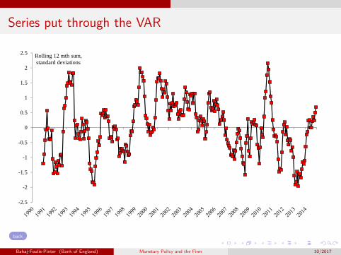
Series put through the VAR

-2.5

-2

-1.5

-1

-0.5

0

0.5

1

1.5

2

2.5 Rolling 12 mth sum, standard deviations

back


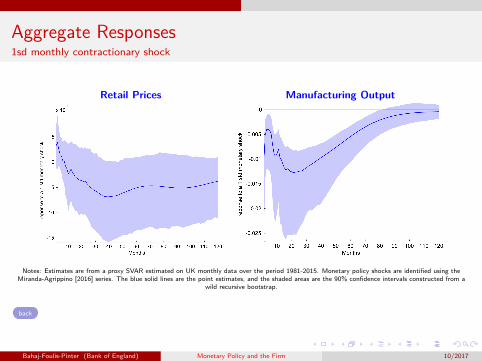
Aggregate Responses1sd monthly contractionary shock

Retail Prices Manufacturing Output

Notes: Estimates are from a proxy SVAR estimated on UK monthly data over the period 1981-2015. Monetary policy shocks are identified using theMiranda-Agrippino [2016] series. The blue solid lines are the point estimates, and the shaded areas are the 90% confidence intervals constructed from a

wild recursive bootstrap.

back


Alternative Estimators


-7

-6

-5

-4

-3

-2

-1

0

1

0 1 2 3 4 5 6 7 8 9 10

Cumulative % Chg

Years since shock

Baseline

Firms who report for 10yrs

WLS estimator

Random Effects Estimator -24

-20

-16

-12

-8

-4

0

4

0 1 2 3 4 5 6 7 8 9 10

Cumulative % Chg

Years since shock

Baseline

Firms who report for 10yrs

WLS estimator

Random Effects Estimator

Notes: Firm level responses to a 1 standard deviation contractionary monetary policy shock. Grey shaded areas are 90% confidence intervals from ourbaseline specification constructed from a tG−1 distribution where G is the minimum of clusters in the regression. Black solid lines with square markers arepoint estimates from a sample where we only include firms who report for 10 years, (ii) black dashed lines with diamond markers are point estimates whenwe weight our baseline regression model by initial number of employees left panel or initial total assets right panel, and (iii) black solid lines with triangularmarkers are point estimates from where we estimate our baseline regressions using a random effects estimator. Left panel: The dependent variable is thecumulative growth rate in log points of employment from t − 1 to t + h where t is the date of the monetary policy shock and h is the x-axis. Right panel:The dependent variable is the cumulative growth rate in log points of in real total assets from t − 1 to t + h where t is the date of the monetary policy

shock and h is the x-axis.

back


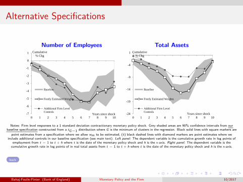
Alternative Specifications


-7

-6

-5

-4

-3

-2

-1

0

1

0 1 2 3 4 5 6 7 8 9 10

Cumulative % Chg

Years since shock

Baseline

Freely Estimated Weights

Additional Firm LevelControls

-24

-19

-14

-9

-4

1

0 1 2 3 4 5 6 7 8 9 10

Cumulative % Chg

Years since shock

Baseline

Freely Estimated Weights

Additional Firm LevelControls

Notes: Firm level responses to a 1 standard deviation contractionary monetary policy shock. Grey shaded areas are 90% confidence intervals from ourbaseline specification constructed from a tG−1 distribution where G is the minimum of clusters in the regression. Black solid lines with square markers are

point estimates from a specification where we allow wm to be estimated, (ii) black dashed lines with diamond markers are point estimates where weinclude additional controls in our baseline specification (see main text). Left panel: The dependent variable is the cumulative growth rate in log points of

employment from t − 1 to t + h where t is the date of the monetary policy shock and h is the x-axis. Right panel: The dependent variable is thecumulative growth rate in log points of in real total assets from t − 1 to t + h where t is the date of the monetary policy shock and h is the x-axis.

back


Alternative Instruments


-8

-7

-6

-5

-4

-3

-2

-1

0

1

2

0 1 2 3 4 5 6 7 8 9 10

Cumulative % Chg

Years since shock

Baseline

Cloyne and Huertgen (2015)

Thwaites, Cesa-Bianchi and Vicondoa (2016)

Miranda-Agrippino (2016) - raw series-23

-18

-13

-8

-3

2

0 1 2 3 4 5 6 7 8 9 10

Cumulative % Chg

Years since shock

Baseline

Cloyne and Huertgen (2015)

Thwaites, Cesa-Bianchi and Vicondoa (2016)

Miranda-Agrippino (2016) - raw series

Notes: Firm level responses to a 1 standard deviation contractionary monetary policy shock. Grey shaded areas are 90% confidence intervals from ourbaseline specification constructed from a tG−1 distribution where G is the minimum of clusters in the regression. Black solid lines with square markers are

point estimates from a model where we identify monetary policy using the Cloyne and Hurtgen [2016] monetary policy series. Black dashed lines withdiamond markers monetary policy identified using Cesa-Bianchi et al. [2016]. Black dashed lines with diamond markers monetary policy identified usingCesa-Bianchi et al. [2016]. Black solid lines with triangular markers are point estimates from where we estimate our baseline regressions using a random

effects estimator.

back


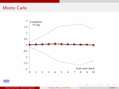
Monte Carlo

-2

-1.5

-1

-0.5

0

0.5

1

1.5

2

0 1 2 3 4 5 6 7 8 9 10

Cumulative % Chg

Years since shock

back


The effect of age: Oldest vs Youngest Firms


-16

-14

-12

-10

-8

-6

-4

-2

0

0 1 2 3 4 5 6 7 8 9 10

Cumulative % Chg

Years since shock

��

��

-30

-25

-20

-15

-10

-5

0

5

0 1 2 3 4 5 6 7 8 9 10

Cumulative % Chg

Years since shock

��

��

Notes: Firm level responses to a 1 standard deviation contractionary monetary policy shock.Comparing oldestand youngest quintile. Dash lines enclose 90% confidence intervals constructed from a tG−1 distribution where

G is the minimum of clusters in the regression.

back


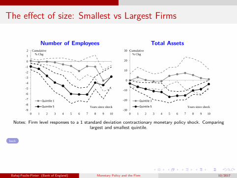
The effect of size: Smallest vs Largest Firms


-9

-8

-7

-6

-5

-4

-3

-2

-1

0

1

2

0 1 2 3 4 5 6 7 8 9 10

Cumulative % Chg

Years since shock

��

��

-30

-20

-10

0

10

20

30

0 1 2 3 4 5 6 7 8 9 10

Cumulative % Chg

Years since shock

��

��

Notes: Firm level responses to a 1 standard deviation contractionary monetary policy shock. Comparinglargest and smallest quintile.

back


Quintiles

Sample I: Employment Sample II: Total AssetsSize (assets £’000s) Age (months) Size (assets £’000s) Age (months)

Q1 77 42 11 36Q2 1109 75 33 63Q3 3677 117 92 107Q4 8986 201 320 188back


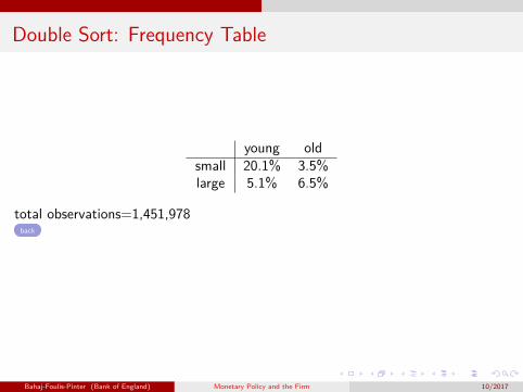
Double Sort: Frequency Table

young oldsmall 20.1% 3.5%large 5.1% 6.5%

total observations=1,451,978back


Measuring ProductivityMeasure I: Labour productivity Ai,t defined as:

Ai,t =Yi,tLi,t

, (2.1)

where Yi,t is real value-added of firm i at time t, and Li,t is the number ofworkers employed by firm i . We deflate with 2-digit SIC code level value-addedprice deflators. Measure II: Total factor productivity TFPi,t : We followWooldridge [2009], Gopinath et al. [2015]) in estimating the followingCobb-Douglas production function:

yi,t = cj + αjki,t + βj li,t + εi,t , (2.2)

c j is an industry FE, yi,t is log real value-added, ki,t is log of real fixed assets, li,t is labour input is log wage bill.We estimate 2.2 with the IV method of Wooldridge [2009] to mitigate theendogeneity of input choices by using intermediate inputs as proxy variablesfor productivity. The log TFP measure for each firm-year observation is givenby the residual εi,t from 2.2.

back


Histogram: Total Assets

7.3e+05

1.4e+05

9.5e+04

6.3e+044.4e+04

3.2e+04 2.4e+04 1.8e+04 1.5e+04 1.2e+04 9979 8298 7111 6261 5408 4667 4042 3683

02.

0e+

054.

0e+

056.

0e+

058.

0e+

05F

requ

ency

0 5000 10000 15000Notes: The data in this graph are truncated at 5% and 95% levels.

firms who report employment

back


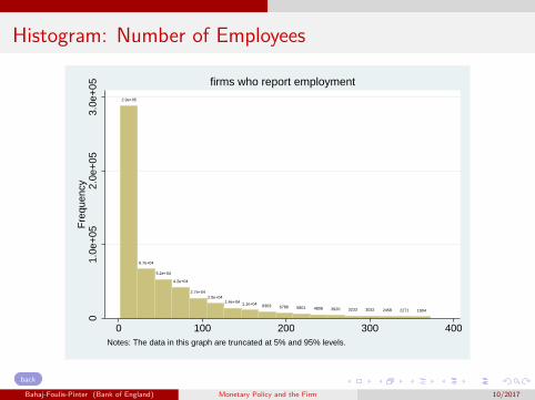
Histogram: Number of Employees

2.9e+05

6.7e+04

5.2e+04

4.2e+04

2.7e+042.0e+04

1.4e+04 1.1e+04 8363 6786 5801 4808 3920 3233 3032 2458 2271 1904

01.

0e+

052.

0e+

053.

0e+

05F

requ

ency

0 100 200 300 400Notes: The data in this graph are truncated at 5% and 95% levels.


back


Histogram: Debt to Assets

1.1e+041.1e+04

1.1e+041.1e+04 1.1e+04

1.1e+04

1.0e+04

8805

7588

6353

5223

4306

3512

2924

2428

19951702

1321

050

001.

0e+

041.

5e+

04F

requ

ency

0 .2 .4 .6 .8Notes: The data in this graph are truncated at 5% and 95% levels.

Mean = .329; Median = .272; N = 136133

back


Histogram: Credit Score

1.2e+06

8.0e+057.3e+05 7.4e+05

1.8e+06

1.2e+06

1.3e+06

2.4e+06

1.2e+06

5.6e+05

6.3e+05

4.2e+05

2.8e+05 2.6e+05

1.9e+05

7.0e+05

1.8e+05

2.6e+05

05.

0e+

051.

0e+

061.

5e+

062.

0e+

062.

5e+

06F

requ

ency

20 40 60 80 100Notes: The data in this graph are truncated at 5% and 95% levels.

firms who report total assets

back


Histogram: Interest Coverage Ratio

51481.2e+04 1.4e+04

2.0e+04

3.3e+04

3.8e+05

2.3e+05

1.0e+05

6.4e+04

4.6e+04

3.0e+04 3.1e+04

1.7e+04 1.9e+041.3e+04 1.1e+04 8883 7297

01.

0e+

052.

0e+

053.

0e+

054.

0e+

05F

requ

ency

-.5 0 .5 1Notes: The data in this graph are truncated at 5% and 95% levels.


back


Histogram: Employment Growth 1-year

4951 34296442 7679

1.1e+04 1.3e+04

2.0e+04

2.8e+04

1.8e+05

3.5e+04

2.9e+04

2.1e+041.6e+04

1.1e+04 95015615 6382

3551

05.

0e+

041.

0e+

051.

5e+

052.

0e+

05F

requ

ency

-.4 -.2 0 .2 .4% growth

Notes: The data in this graph are truncated at 5% and 95% levels.


back



12632399

3460

6745 5973

9867

1.5e+04

1.8e+042.0e+04

8.4e+04

2.3e+04

2.0e+04

1.4e+04

9685 9196

57793993

2497

02.

0e+

044.

0e+

046.

0e+

048.

0e+

04F

requ

ency

-1 -.5 0 .5 1% growth



back



1298

3844

2307

3519

6330

8212

1.1e+04

3.1e+04

1.3e+041.3e+04

1.1e+04

8619

6476

43824796

26132028 1822

01.

0e+

042.

0e+

043.

0e+

04F

requ

ency

-1 -.5 0 .5 1% growth



back



539 553

802

1609

1887

3174

3972

7558

54065281

4385

3277

2882

1889

1456

1067848

583

020

0040

0060

0080

00F

requ

ency

-1 0 1 2% growth



back


Histogram: Total Assets

9.0e+06

1.9e+06

9.4e+05

6.1e+054.3e+05

3.2e+05 2.6e+05 2.1e+05 1.7e+05 1.5e+05 1.2e+05 1.0e+05 9.3e+04 8.3e+04 7.2e+04 6.8e+04 5.8e+04 5.2e+04

02.

0e+

064.

0e+

066.

0e+

068.

0e+

061.

0e+

07F

requ

ency

0 500 1000Notes: The data in this graph are truncated at 5% and 95% levels.


back


Histogram: Asset Growth 1-year

9.4e+04

2.4e+051.9e+05

2.6e+05

3.8e+05

4.9e+05

7.2e+05

1.0e+06

2.6e+06

1.3e+06

9.8e+05

7.5e+05

5.0e+05

4.3e+05

3.0e+05

2.1e+05 2.4e+05

1.3e+05

05.

0e+

051.

0e+

061.

5e+

062.

0e+

062.

5e+

06F

requ

ency

-1 -.5 0 .5 1% growth



back



1.1e+05 1.1e+05

1.6e+05

2.5e+052.8e+05

4.0e+05

5.4e+05

7.3e+05

1.4e+06

8.0e+05

6.7e+05

5.2e+05

4.0e+05

3.4e+05

2.4e+05

1.7e+051.6e+05

1.1e+05

05.

0e+

051.

0e+

061.

5e+

06F

requ

ency

-1 -.5 0 .5 1 1.5% growth



back



6.1e+04

8.8e+049.9e+04

1.3e+05

1.9e+05

2.4e+05

3.1e+05

4.0e+05

6.3e+05

4.1e+05

3.6e+05

3.1e+05

2.3e+05

1.8e+05

1.5e+05

1.2e+05

9.1e+04

6.1e+04

02.

0e+

054.

0e+

056.

0e+

05F

requ

ency

-2 -1 0 1 2% growth



back



1.9e+04

2.6e+04

3.2e+04

4.2e+04

5.9e+04

7.5e+04

9.8e+04

1.6e+05

1.2e+051.2e+05

1.1e+05

9.4e+04

8.0e+04

6.3e+04

4.9e+04

3.8e+04

3.0e+04

2.3e+04

05.

0e+

041.

0e+

051.

5e+

05F

requ

ency

-2 -1 0 1 2% growth



back


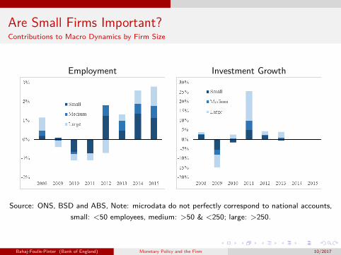
Are Small Firms Important?Contributions to Macro Dynamics by Firm Size

Employment Investment Growth

Source: ONS, BSD and ABS, Note: microdata do not perfectly correspond to national accounts,small: <50 employees, medium: >50 & <250; large: >250.


monetarypolicyandthefirm: someempiricalevidence1 · share of total jobs (%) ... url....

Documents