Money, Deficits, Debts and Inflation in Emerging Countries: Evidence from Turkey

Amir Kia

Finance and Economics Department Utah Valley University Orem, UT 84058-5999

USA

Tel: (801) 863-6898 Fax: (801) 863-7218

E-mail:akia@uvu.edu

Abstract: This paper focuses on internal and external factors, which influence the inflation rate in Turkey. The monetary model of inflation rate which was developed by Kia (2006a) was extended and tested on Turkish data. It was found that government debt and deficits along with other factors are important determinants of inflation in Turkey. Furthermore, most sources of inflation in this country are domestic factors. Keywords: Outstanding debt, deficit, inflation, fiscal and monetary policies, external and

internal factors

JEL Codes: E31, E41, E50 and E62

Money, Deficits, Debts and Inflation in Emerging Countries: Evidence from Turkey

I. Introduction

The objective of this paper is to investigate empirically the monetary (including

real exchange rate) and fiscal (including outstanding public debt, debt management,

deficits and government expenditure) as well as other determinants of inflation rate in

Turkey. To the best knowledge of the author, except for Kia’s (2006a) work which is on a

non-traditional economy, no such study for emerging or developed countries exists. For

example, Togan (1987), using a monetary approach to inflation, finds the real income has

a positive impact on the inflation rate, while the real interest rate, depending on the

estimation technique, may have a positive or a negative impact on the inflation rate in

Turkey. Dornbush et al. (1990) and Drazen and Helpman (1990) find that an uncertainty

on the time when the deficits are financed creates fluctuation in the inflation rate.

Bahmani-Oskooee (1995) finds the world price has a positive impact over the long run on

the consumer price in Iran. Özatay (1997) finds that when the fiscal process is not

sustainable, the monetary policy cannot be independent and, therefore, because of an

unsustainable fiscal policy, price stability in Turkey is very difficult to achieve.

Furthermore, Lim and Papi (1997), using an ad hoc general equilibrium model,

find the exchange rate and the public deficit have a negative impact on the inflation rate,

but the money supply causes a higher inflation rate in Turkey. Pongsaparn (2002), using

an ad hoc small scale macroeconomic model, tests the impact of macroeconomic

variables like domestic and foreign interest rates, real exchange rate, broad money supply

and debt-to-GDP ratio on the price level/inflation rate in Turkey. This study finds the

2 domestic interest rate has a negative impact on the price level, but other variables,

including the outstanding debt per GDP, have a positive impact on the price level in

Turkey.1 Tekin-Koru and Ozmen (2003) find no support for the linkage between the

budget deficit and inflation through the wealth effect in Turkey. Instead, they found that

deficit financing leads to a higher growth of interest-bearing broad money, but not

currency seigniorage. Us (2004) finds the consumer price index causes monetary base,

but the reverse is not true in Turkey. Arize et al. (2004) find that the inflation in

82 countries responds positively to the volatility of real and nominal exchange rates.

Berument and Kilinc (2004) find shocks in the industrial production of Germany, the

United States and the rest of the world will affect positively the inflation rate in Turkey.

Ashra et al. (2004), using a monetary approach to inflation, investigate a causality

relationship between deficit, money supply and inflation in India. They found no

relationship between the central bank credit to the government and the government

deficit, but found that M3 causes the inflation rate.

El-Sakka and Ghali (2005) find the nominal exchange rate, the nominal interest

rate, the money supply and the world price have a positive impact on the consumer price

index in Egypt but the real income has a negative impact on the level of price.

Kia (2006a) finds, over the long run, a higher exchange rate (lower value of domestic

currency) leads to a higher price in Iran, a higher money supply when it is anticipated

does not lead to a higher price level, but an unanticipated shock in the money supply

results in a permanent rise in the price level. He also finds that the real government

expenditures as well as deficits cause inflation, but if the changes are unanticipated they

3

cause the opposite effect. Furthermore, a high debt per GDP is deflationary and the

foreign financing of the government debt has no price impact when it is anticipated, but it

has a positive effect if unanticipated. The foreign interest rate has a deflationary effect in

Iran over the long run while imported inflation does not exist in that country.

Rabanal (2007), using a dynamic stochastic general equilibrium model, shows a

tight monetary policy in the United States results in a higher inflation rate through a cost

of capital. Boschi and Girardi (2007) attempt to find short-run and long-run determinants

of the inflation rate in the Euro Area. They found that both demand and supply-side

factors, through mark-up process and output gap, affect inflation. Tawadros (2007) uses a

monetarist model of inflation to test the neutrality of money in Egypt, Jordan and

Morocco and finds that money affects inflation in these countries and not the real income.

Berument (2007), using a VAR model, finds that tight monetary policy reduces income

and prices, but results in an appreciation of domestic currency in Turkey. Finally,

Williams and Adedeji (2007), using a monetary approach to inflation, find that the

inflation rate in the Dominican Republic is affected by money supply, real income,

foreign inflation as well as the exchange rate. However, none of these studies

incorporates completely the direct impact of the government spending, deficits, the

outstanding debt and the government debt management on the inflation rate. As we saw

above, some of these studies incorporated one or more public variables while ignoring the

rest.

Furthermore, excluding Kia (2006a), no study on estimating the cointegration

relationship so far allows the short-run dynamics of the system to be influenced by policy

1 Both Lim and Papi (1997) and Pongsaparn (2002) provide a survey on empirical studies on inflation in

4

regime changes as well as other exogenous shocks. As evidenced by Kia (2006b),

constant models can have time-varying coefficients if a deeper set of constant parameters

characterizes the data generation process. Specifically, the existence of constancy may

depend on whether raw coefficients or underlying parameters are evaluated. Kia (2006b)

also shows that the estimated long-run relationship can be biased when the appropriate

policy regime changes and/or other exogenous shocks are not incorporated in the

short-run dynamics of the system. This fact is especially important for the studies on

Turkish inflation since the country has witnessed several changes in policy regimes and

undergone many other exogenous shocks during the past three decades. For example, in

the 1980’s Turkey moved from an import-substitution policy to an export-incentives

policy. Some studies, e.g., Lim and Papi (1997), consider this policy regime change a

long-run structural break in the estimation of an inflation equation for Turkey. However,

as we will see in this paper such a policy change did not generate any structural break in

the long-run cointegration relationship.

To fill the gap in this literature, we extended Kia’s (2006a) model and tested it on

the Turkish data and the estimation results proved the validity of the extended model, as

it is unique in this literature. It should be noted that the model used in this study is

different than Kia’s model. The extended model used in this paper is for a country (i.e.,

Turkey) which is operating under conventional economics. Specifically, our tested model

includes the domestic interest rate as well as the real rather than the nominal exchange

rate and imposes the restrictions implied by the theoretical model.

Turkey.

5

Turkey, which relies mostly on agricultural products, experienced severe

inflation, up to 106.6% in 1994, when the outstanding debt was 44% of GDP. The

outstanding debt reached 99.87% of GDP in 2001 when the inflation rate was 54.4%. The

model used in this study is an augmented version of the monetarist model which, unlike

the model used in the existing literature, is designed in such a way to incorporate both

external and internal factors, which cause inflation in the country. Furthermore, since the

model also incorporates government deficits and debt, we could test Sargent and

Wallace’s (1986) views that (i) the tighter is the current monetary policy, the higher

inflation rate will eventually be, and (ii) that government deficits and debt will eventually

be monetized in the long run.

It was found that the model is successful in capturing the impact of fiscal

instruments, i.e., deficits, debt and debt management, and of monetary instruments on the

inflation rate in Turkey. Furthermore, a policy toward a stronger currency is inflationary

and most sources of inflation in Turkey are domestic factors. Finally, Sargent and

Wallace’s view on a tight monetary policy leading to higher inflation over the long run is

valid. As for fiscal variables in Turkey, it was found that a higher government debt per

GDP results in a riskier environment and, therefore, in a higher rate of inflation.

However, the reverse is true for the externally government debt financing over the long

run. Moreover, there is no imported inflation in Turkey over the long run.

The following section deals with the development of the theoretical model.

Section III describes the data and the long-run empirical methodology and results.

Section IV is devoted to the short-run dynamic models, which is followed by a section on

6 analyzing the impact of unanticipated shocks on the inflation rate. The final section

provides some concluding remarks.

II. The Model

Considers an economy with a single consumer, representing a large number of

identical consumers. The consumer maximizes the utility function (1) subject to budget

constraint (2), where

U(ct, ct*, gt, ktmt, mt*) = (1- α)-1 (ctα1

c*t α2

gt α3)1-α

+ ξ (1- η) –1[(mt/kt) η1 m*tη2]1-η, (1)

τt + yt + (1 + πt)-1 mt-1 + qt (1 + π*t)-1 m*t-1 + (1 + πt)-1 (1 + Rt-1) dt-1 +

qt (1 + π*t)-1 (1 + R*t-1) d*t-1 = ct + qt ct* + mt + qt mt* + dt + qt dt*, (2)

where τt is the real value of any lump-sum transfers/taxes received/paid by consumers, qt

is the real exchange rate, defined as Et pt*/pt, Et is the nominal market exchange rate

(domestic price of foreign currency), pt* and pt are the foreign and domestic price levels

of foreign and domestic goods, respectively, yt is the current real endowment (income)

received by the individual, m*t-1 is the foreign real money holdings at the start of the

period, dt is the one-period real domestically financed government debt which pays R rate

of return and dt* is the real foreign issued one-period bond which pays a risk-free interest

rate Rt*, where dt and dt* are the only two storable financial assets.

It is assumed variable kt, which summarizes risk associated to holding domestic

money, has the following long-run relationship:

log (kt) = k0 defgdpt + k1 debtgdpt + k2 fdgdpt. (3)

Variables defgdp, debtgdp and fdgdp are real government deficits per GDP, the

government debt outstanding per GDP and the government foreign-financed debt per

7 GDP, respectively, where it is assumed government debt pays the same interest rate as

deposits at the bank (i.e., R).

Equation (3) is also assumed to be held subject to a short-run dynamics system,

which is a function of a set of predetermined short-run (stationary) variables known to

individuals. These variables include the growth of money supply, changes in fiscal

variables per GDP, the growth in exchange rate, domestic and foreign inflation as well as

changes in interest rates. Furthermore, it is assumed that the short-run dynamics of the

risk variable [log (k)] includes a set of interventional dummies which account for wars,

sanctions, political changes, innovations as well as policy regime changes which

influence services of money. Maximizing the utility function (1) subject to equations (2)

and (3) and imposing some stability conditions, Kia (2006a) finds the following demand

for money relationship:

log(mt) = m0 + m1 it + m2 log(yt) + m3 log(g t) + m4 log(k t) + m5 log(qt)

+ m6 i*t, (4)

where, i*t = log(R*t/1+ R*t), it = log(Rt/1+ Rt) and, m0 >0, m1 <0, m2 >0,

m3 < 0, m4 <0, m5 =?, m6 < 0. From the equilibrium condition in the money market we

can find the following price relationship:

lpt = β0 + (β1=1) lMst + β2 it + β3 lyt + β4 lqt + β5 i*t + β6 lgt + β7 defgdpt

+ β8 debtgdpt + β9 fdgdpt + β10 trend + ut, (5)

where an l before a variable means the logarithm of that variable and u is a disturbance

term assumed to be white noise with zero mean. βs are the parameters to be estimated,

where β1 = 1, β2 >0, β3 <0, β4 =?, β5 >0, β6 >0, β7 >0, β8 >0, β9 >0 and β10 >0. It should

be noted that Equation (5) is very different from the price equation estimated by

8 Kia (2006a). He assumed it is zero so as to be able to estimate the equation on Iranian

data. Furthermore, Kia substituted for the real exchange rate (lqt) its components (i.e., Et

pt*/pt) and, therefore, his tested model is a function of the nominal exchange rate as well

as the foreign price rather than the real exchange rate.

Consequently, he needed to impose two important restrictions on the coefficients

of his model: (i) making the coefficient of the nominal exchange rate and the level of

foreign price equal and (ii) the summation of the coefficient of money supply and

nominal exchange rate (or foreign price) equal to one. Since these two restrictions make

an estimate of the long-run price level unrealistic, he estimated the long-run model

without any restriction. However, in our model we only need to impose β1=1.

Furthermore, foreign price in terms of the domestic price (real exchange rate) is a more

appropriate determinant of the price level over the long run than its absolute value.

Therefore, Equation (5) is a more valid equation for a country like Turkey, where the

economy has been operating under a traditional economic system. The next section of

this paper is devoted to such estimation.

According to the model, a higher money supply and a higher interest rate (tight

monetary policy) increase the price level over the long run. This confirms the theoretical

model of Sargent and Wallace’s (1986, p. 160) view that ‘[…] given the time path of

fiscal policy and given that government interest-bearing debt can be sold only at a real

interest rate exceeding the growth rate n, the tighter is current monetary policy, the higher

must the inflation rate be eventually.’ A higher real income results in a higher real

demand for money and a lower price level. We cannot determine theoretically the impact

of the exchange rate and the foreign price level on the domestic price level. According to

9 our model, the impact of deficit, government spending, outstanding government debt and

debt financed externally, for a given output level, on the price level is positive.

Consequently, these fiscal variables, according to our theoretical model, are inflationary.

Note that since the real government expenditure is considered a “good” - in fact, a public

good - its level influences the price, while deficits and debt are measures for future taxes

and inflation, and so their proportions to GDP may influence the price level. The

estimation result of the model on Turkish data, which is generated by traditional

economics, is given in the next section.

III. Data, Long-Run Empirical Methodology and Results

(A) Data

The model is tested for Turkey (1970Q1-2003Q3). All observations are quarterly

and the sample period is chosen according to the availability of the data. The sources of

the data, unless specified, are the International Financial Statistics (IFS) online. Some

missing data were taken from the World Development Indicator (WDI) and some from

the State Institute of Statistics of Turkey (SIS) or IMF – Economic and Financial Data

for Turkey. Data series on GDP, government deficits and expenditures as well as debt

financed externally and outstanding government debt are only available yearly. Quarterly

observations were, consequently, interpolated using the statistical process developed by

RATS. This procedure keeps the final value fixed within each full period.

Information on institutional and policy changes in Turkey were taken from The

Middle East and North Africa (2004). lp is the logarithm of Consumer Price Index (CPI),

lMs is the logarithm of nominal M1, i is the logarithm of (R/1+R), where R is the

discount rate at the annual rate, in decimal points. Note that the only reason, as a measure

10 for the domestic interest rate, the discount rate was chosen is because of its data

availability in the sample period. Quarterly data on other more relevant interest rates is

only available for a very short part of the sample period. For instance, Treasury Bills

rates are available only from 1985Q4.

Variable y is the real GDP, which is the nominal GDP divided by CPI. Variable g

is the real (nominal deflated by CPI) government expenditures on goods and services,

q=Ep*/p is the real exchange rate, where E is the nominal market exchange rate, which is

equal to the domestic currency in terms of $US. Variable p* is the foreign price level

where, following Kia (2006a) among others, the industrial countries unit value export

price index was used as a measure for p*. Foreign rate i* is the logarithm of (R*/1+R*),

where, following Kia (2006a), R* is the LIBOR (3-month London interbank) rate at the

annual rate, in decimal points. Variables defgdp, debtgdp and fdgdp are deficits,

outstanding debt and foreign debt per GDP, respectively.

(B) Stationarity Tests

To investigate the stationarity property of the variables I used Augmented

Dickey-Fuller (ADF) and non-parametric Phillips-Perron’s (PP) tests. Furthermore, the

LM unit root test developed by Schmidt and Phillips (1992), (SP, hereafter), was used.

This test, in contrast to the Dickey-Fuller test, allows for trend under both the null and the

alternative, without introducing any parameters that are irrelevant under either.

I found all variables, except the government expenditure on goods and services

are integrated of order one according to all test results (i.e., the level of these variables

has a unit root, but their first differences are stationary). The government expenditure on

11 goods and services, however, was found to be stationary based on all test results. For the

sake of brevity, these results are not reported, but are available upon request.

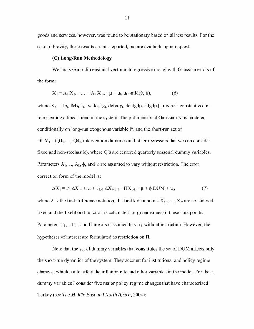
(C) Long-Run Methodology

We analyze a p-dimensional vector autoregressive model with Gaussian errors of

the form:

X t = A1 X t-1+… + Ak X t-k+ μ + ut, ut ~niid(0, Σ), (6)

where X t = [lpt, lMst, it, lyt, lqt, lgt, defgdpt, debtgdpt, fdgdpt], μ is p×1 constant vector

representing a linear trend in the system. The p-dimensional Gaussian Xt is modeled

conditionally on long-run exogenous variable i*t and the short-run set of

DUMt = (Q1t, …, Q4t, intervention dummies and other regressors that we can consider

fixed and non-stochastic), where Q’s are centered quarterly seasonal dummy variables.

Parameters A1,…, Ak, φ, and Σ are assumed to vary without restriction. The error

correction form of the model is:

ΔX t = Γ1 ΔX t-1+… + Γk-1 ΔX t-k+1+ ΠX t-k + μ + φ DUMt + ut, (7)

where Δ is the first difference notation, the first k data points X t-1,…, X 0 are considered

fixed and the likelihood function is calculated for given values of these data points.

Parameters Γ1,...,Γk-1 and Π are also assumed to vary without restriction. However, the

hypotheses of interest are formulated as restriction on Π.

Note that the set of dummy variables that constitutes the set of DUM affects only

the short-run dynamics of the system. They account for institutional and policy regime

changes, which could affect the inflation rate and other variables in the model. For these

dummy variables I consider five major policy regime changes that have characterized

Turkey (see The Middle East and North Africa, 2004):

12

(i) In 1984Q4, the government introduced a value-added tax to replace the

previous unwieldy system of production taxes. Furthermore, the capital account

liberalization started in 1984, when the foreign exchange rate regime was liberalized.

Banks were allowed to offer foreign currency-denominated account and non-residents

could open lira-denominated accounts in Turkey. Residents could also buy and sell

foreign-denominated securities. In other words, capital mobility was allowed. This policy

resulted in an appreciation of the Turkish lira [see Pongsaparn (2002) on capital account

liberalization].

(ii) In January 1994, two U.S. credit rating agencies downgraded Turkey's credit

rating, which resulted in a run of foreign currencies. The value of the lira was officially

devalued by 12% against the US dollar; however, the currency continued to plummet.

Interest rates rose to 150% - 200% as the government and the Central Bank desperately

tried to bring the financial markets under control. In April 1994, the government

announced a program of austerity measures to reduce the budget deficit, lower inflation

and restore domestic and international confidence in the economy. The program included

a freezing of wages, price increases of up to 100% on state monopoly goods, as well as

longer-term restructuring measures such as the closure of loss-making state enterprises

and an accelerated privatization process.

(iii) In July 1995, the new government approved a raise in the minimum wage and

salary increases of 50% for state workers and pensioners. The government stated that the

main aspects of its economic program were a commitment to a free-market economy,

lower inflation and a steady growth rate, lower taxation for producers, greater efforts to

13 attract foreign investment, an acceleration in the privatization program and an emphasis

on investment in infrastructure projects.

(iv) In January 2000, as part of the anti-inflation program, a new exchange rate

substitution policy took effect under which the managed peg used since 1994 was

abandoned in favor of a peg set according to a pre-determined devaluation rate (20% in

2000), itself set against a basket of the US dollar and the euro.

(v) In February 2001, following a public clash between the President and the

Prime Minister, the financial system went into near-meltdown in Turkey's worst

economic crisis in recent years. A massive flight of capital forced the government to float

the lira and accept an immediate devaluation of the currency. Consequential consumer

price increases sparked widespread protest demonstrations, amidst rumors that another

military takeover was imminent. The interest rate rose to the equivalent of 4,000%

annually. On February 22, 2001, the government ended the crawling peg with the US

dollar and allowed the lira to float freely, with the result that its value fell by 36% over

two days. Accordingly, I use the following dummy variables to represent these potential

policy regime shifts and exogenous shocks: vtax = 1 from 1984Q4 and = 0, otherwise,

fcrisis = 1 for 1994Q2 and = 0, otherwise, pwd = 1 for 1995Q2-1995Q3 and = 0,

otherwise, MEX = 1 for 1994Q4-1999Q4 and = 0, otherwise, PEX = 1 for 2000Q1-

2000Q4 and = 0, otherwise, flex = 1 since 2001Q1 and = 0, otherwise. One may also

argue that, e.g., Lim and Papi (1997), when Turkey moved from an import-substitution

policy in the 1980’s to an export-incentives policy, it created a structural break in the

long-run inflation relationship. We will show that there is no structural break in our

cointegration relationship.

14

In determining the lag length one should verify if the lag length is sufficient to get

white noise residuals. As it was recommended by Hansen and Juselius (1995, p. 26), set

p=r (the unrestricted model) in Equation (6) and test for autocorrelation. In this case the

residuals are the OLS-estimates from Model (6). LM tests will be employed to confirm

the choice of lag length. The order of cointegration (r) will be determined by using the

Trace test developed in Johansen and Juselius (1991). Following Cheung and Lai (1993),

the Trace test will be adjusted in order to correct a potential bias possibly generated by a

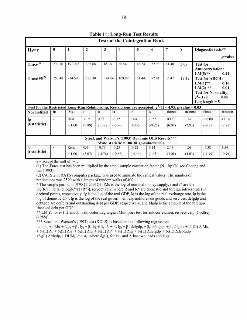
small sample error. Table 1 reports the result of the Trace test as well as the estimated

long-run relationships of Equation (5).

Table 1 about here

According to diagnostic tests reported in the table, the lag length 5 was sufficient

to ensure that errors are not autocorrelated. According to normality test results, the error

is not normally distributed. However, as it was mentioned by Johansen (1995), a

departure from normality is not very serious in cointegration tests. Since we allow the

short-run dynamics of the system to be affected by the dummy variables included in

vector DUM we need to simulate the critical values as well as their associated p-values

for the rank test. CATS in RATS computer package [Version 2, see Dennis (2006)] was

used to simulate the critical values. The number of replications is 2500 and the length of

random walks is 400.

According to the Trace test result reported in Table 1 we can reject r=0 at 5%

level, while we cannot reject r≤1, implying that r=1. Figure 1 plots the calculated values

of the recursive test statistics for the long-run relationship. Note that these statistics are

recursive likelihood-ratios normalized by the 5% critical value. Thus, calculated statistics

15 that exceed unity imply the rejection of the null hypothesis and suggest unstable

cointegrating vectors. The broken line curve (BETA_Z) plots the actual disequilibrium as

a function of all short-run dynamics including seasonal dummy variables, while the solid

line curve (BETA_R) plots the “clean” disequilibrium that corrects for short-run effects.

We hold up the first fifteen years for the initial estimation. As the figure shows, the

relationship appears stable over the long run when the models are corrected for short-run

effects. To investigate if moving from the import-substitution policy to the

export-incentives policy in 1983Q4 [see Lim and Papi (1997)] resulted in a structural

break in our cointegration relationship I went through the above exercise by allowing a

break in 1983Q4. The estimated coefficient was -0.29 with a t-statistic of -1.54 which

implies there is no structural break as a result of this policy regime shift.

Figure 1 about here

For the sake of robustness, the dynamic OLS (DOLS) test of Stock and

Watson (1993) was also used to estimate the above long-run equation (Equation (5)). For

the sake of brevity, the bottom panel of Table 1 reports only the estimated result for the

price equation (Equation (5)). See the footnote of the table indicated by *** for the

formula. The DOLS Wald test result, reported in the table, also indicates the existence of

a long-run cointegrated relationship in the space. Comparing the estimated result with the

long-run estimated relationship, using MLS procedure we can see that the estimated

coefficients of the real income and foreign interest rate are now statistically significant,

but with a different sign. Moreover, the estimated coefficient of the real government

expenditure is now statistically insignificant, but again has a different sign. All other

coefficients have the same sign, but the coefficient of the real exchange rate is

16 statistically insignificant under DOLS while the estimated coefficient of deficit per GDP

is statistically significant under DOLS estimation method.

The estimated coefficients of other variables in DOLS, which only affect the

short-run dynamics of the system, for the sake of brevity, are not reported, but are

available upon request. The differences between these two long-run estimated results are

due to the fact that the DOLS result is less efficient and less reliable than the estimated

result of the MLS procedure. Having established that a long-run and stable relationship

exists, we will analyze these long-run equations.

(D) Long-Run Relationship

(i) Monetary policy: According to our theoretical model [Equation (5)], we would

expect interest rate to have a positive influence on the price level. Based on our

estimation result, the interest rate has a positive and a statistically significant impact on

the price level. This means that a tight monetary policy when debt and deficits exist leads

to a higher inflation over the long run in Turkey, i.e., Sargent and Wallace’s (1986) view

that “[…] the tighter is current monetary policy, the higher must the inflation rate be

eventually” cannot be rejected at least for Turkey. This means that, given the time path of

fiscal policy and the fact that interest-bearing government debt can be sold only at a real

interest rate exceeding the growth rate of the economy, a current tight monetary policy in

Turkey results in a higher inflation over the long run. This result confirms

Pongsaparn’s (2002) and Baydur and Süslü’s (2004) finding. However, Baydur and

Süslü’s analysis is mostly a short-term study, while our finding is a long-run conclusion.

Considering the exchange rate as a monetary instrument, a depreciation of the

domestic currency (appreciation of exchange rate) in Turkey leads to a fall in the price

17 level, as the coefficient of the real exchange rate indicates in the price equation. Note that

a higher E in variable q means a depreciation of domestic currency. This result confirms

Pongsaparn’s (2002) finding. So far, we found the domestic monetary policy, including

the exchange rate policy, could be a major tool to fight inflation over the long run in

Turkey. For example, an easy monetary policy which results in a lower interest rate leads

to a lower inflation rate over the long run when debt and deficit exist. Furthermore, a

depreciation of the domestic currency leads to a higher demand for money (a lower

demand for goods and services) resulting in a downward pressure of the price level over

the long run.

(ii) Fiscal policy: The long-run estimated coefficient of the log of the real

government expenditure is negative and statistically significant. This result implies that

over the long-run, a higher government expenditure results in a higher demand for money

and, therefore, has a depressing impact on the price level. To the best knowledge of the

author, no study has dealt with the impact of the government expenditures on the price

level for Turkey and so comparison is not possible. However, Kia (2006a) finds a higher

government expenditure in Iran lead to a higher price level over the long run, as the

model predicts.

The long-run estimated coefficient of deficits per GDP is positive, but is

statistically insignificant. This result confirms our theoretical model. The result is

consistent with the finding of Tekin-Koru and Ozmen (2003). The estimated coefficient

of the government debt per GDP is positive and statistically significant, confirming the

theoretical model. This implies that a higher government debt in Turkey is associated

with a riskier environment and higher inflation. This result is consistent with the finding

18 of Pongsaparn (2002). The estimated coefficient of the externally financed government

debt per GDP is negative and statistically significant. This result implies that a rise in a

foreign financing of debt reduces the risk in holding domestic money and so leads to

lower inflation. However, as we will see later in this paper the situation is different over

the short run.

(iii) External factors: The foreign interest rate has a positive, but statistically

insignificant impact on the price. The estimated long-run coefficient of the real exchange

rate is negative and statistically significant. Noting that we could not determine

theoretically the sign of the real exchange rate in the price equation, the negative impact

of the real exchange rate on price, for a given nominal exchange rate, means a negative

impact of the foreign price on the domestic inflation rate. This means contrary to the case

of Iran [see Bahmani-Oskooee (1995) and Kia (2006a)] and the Dominican Republic [see

Williams and Adedeji (2007)] there is no imported inflation over the long-run in Turkey.

Furthermore, as the nominal exchange rate goes up (Turkish lira depreciates), the price

will fall. This result confirms Pongsaparn’s (2002) finding, but it contradicts Lim and

Papi’s (1997) finding. Finally, the estimated coefficient of the real GDP, contrary to the

model is positive, but statistically insignificant.

19 IV. Short-Run Dynamic Models of Inflation Rate

In this section we specify the ECM (error correction model) that is implied by our

cointegrating vector, estimated in previous section. Following Granger (1986), we should

note that if small equilibrium errors can be ignored, while reacting substantially to large

ones, the error correcting equation is non linear. All possible kinds of non linear

specifications, i.e., squared, cubed and fourth powered of the equilibrium errors (with

statistically significant coefficients) as well as the products of those significant

equilibrium errors were included.

Note that the error-correction term is a generated variable and its t-statistic should

be interpreted with caution [Pagan (1984)]. To cope with this problem, I implemented,

following Pagan (1984), the instrumental variable estimation technique, where the

instruments were first and second lagged values of the error term. Furthermore, to avoid

biased results, I allowed for a lag profile of four quarters. And, to ensure parsimonious

estimations, I selected the final ECMs on the basis of Hendry’s General-to-Specific

approach. Since there are eight endogenous variables in the system, we may have eight

error-correction models. However, for the sake of brevity, I only report the parsimonious

reduced form and the structural form of ECM for the inflation rate. Other results are

available upon request.

Some of these variables were found to have only a marginal model instead of

ECM. Specifically, the error-correction term was found to be statistically insignificant in

the model for the deficit per GDP (defgdp), the outstanding debt per GDP (debtgdp) and

the foreign-financed debt per GDP (fdgdp). In fact, the deficit and the foreign-financed

debt per GDP were found to be strongly exogenous. It should be mentioned that for any

20 cointegrating relationship there should be at least one ECM and in the above model we

have five ECMs. Tables 2 and 3 assemble the parsimonious results from the estimating

structural and reduced forms of ECM. Other models are available upon request. The

structural equation is estimated by the two-stage least squares method by allowing the

fitted value of each contemporaneous variable from a parsimonious marginal model [for

the definition of marginal model, see Engle, Hendry and Richard (1983), Engle and

Hendry (1993) and Kia (2003a and 2003b)] based on four lag values of all variables in

the system to serve as its own instruments. To construct overidentified equations,

following Johansen and Juselius (1994), I first estimated the correlation coefficients

between endogenous variables. Then by imposing a zero restriction on the coefficient of

variables in any equation with a correlation coefficient of less than 0.20, in the absolute

value term, with the dependent variable, the overidentified structural equations were

constructed. The estimated coefficients of the structural equations may not be

asymptotically efficient and other estimation methods, e.g., three-stage least squares or

full information maximum likelihood estimators are more appropriate, but because of the

lack of enough observations I was unable to use these estimators.

In tables 2 and 3, White is White’s (1980) general test for heteroskedasticity,

ARCH is five-order Engle’s (1982) test, Godfrey is five-order Godfrey’s (1978) test,

REST is Ramsey’s (1969) misspecification test, Normality is Jarque-Bera’s (1987)

normality statistic, Li is Hansen’s (1992) stability test for the null hypothesis that the

estimated ith coefficient or variance of the error term is constant and Lc is Hansen’s

(1992) stability test for the null hypothesis that the estimated coefficients as well as the

error variance are jointly constant. None of these diagnostic checks is significant.

21 According to Hansen’s stability test result, all of the coefficients, individually or jointly,

are stable. Both level and interactive combinations of the dummy variables included in

the set DUM were tried for the impact of these potential shift events in the models. As it

was mentioned in the previous section, DUM also appeared in the short-run dynamics of

the system in our cointegration regression.

Tables 2 and 3 about here

According to our estimation results reported in tables 2 and 3, the error-correction

term is significant and non-linear, implying that individuals in Turkey may ignore a small

deviation from equilibrium, but react drastically to a large deviation. According to the

result in Table 2, the growth of the real GDP has an instantaneous impact on the inflation

rate. The estimated coefficient of the growth of the real GDP is negative as the theoretical

model predicts, but after a quarter, as the estimated coefficient of the lag value indicates,

is positive implying that after a quarter a higher income leads to a higher demand for

goods and services and causes a higher inflation rate. The latter result can also be seen

from the reduced form of the ECM reported in Table 3. This result confirms

Pongsaparn’s (2002) finding. As the estimated coefficient of lagged values of the growth

of the real government expenditure (Table 3) indicates, the growth of the real government

expenditure leads to a higher inflation rate in the country up to two quarters. This positive

relationship confirms the theoretical model [Equation (5)].

The estimated coefficient of the change in interest rate is negative after three

quarters (tables 2 and 3), but over the long run, as we saw (Table 1), a higher interest rate

is associated with a higher price level. Namely, a higher interest rate (a tight monetary

policy) reduces the inflation rate after three quarters, but will cause it to go up over the

22 long run (Table 1). Pongsaparn (2002) also finds a negative relationship between interest

rate and inflation over the short-run in Turkey. Furthermore, Telli, et al. (2008), using

simulation, find a lower interest rates leads to inflationary pressures on commodity and

financial markets in Turkey.

According to the estimated coefficient of the growth of the government

expenditure, an increase in the size of the government results in a higher inflation rate in

Turkey. As for policy regime or institutional change, according to the estimated

coefficient of the dummy variable fcrisis, the financial crisis of 1994 had a positive shock

on the inflation rate in Turkey while the anti-inflation program of January 2000 which

resulted in banning managed peg exchange rate and allowing the lira to float freely on

February 22, 2001 resulted in a lower inflation rate in Turkey, see the estimated

coefficient of dummy variables peg and flex, respectively.

As for external factors, according to the estimated coefficient of the foreign rate

of interest, in both structural and reduced forms of ECM, after two lags this rate has a

positive impact on the inflation rate. Specifically, it seems the inflation in emerging

countries is partly due to a higher foreign interest rate as Kia (2006a) also finds a similar

result for Iran. Dummy variables Nor1980Q1Q2 and Nor1988Q1, which account for

outliers in the data, have positive estimated coefficients. Nor1980Q1Q2 may account for

the start of the capital account liberalization in 1980. Nor1988Q1 accounts for the

deposit-interest rates liberalization, see Pongsaparn (2002), for these two policy regime

changes. The overall conclusion is that the sources of inflation in Turkey are both internal

and external factors.

23 V. Unanticipated Shocks

The estimated coefficients of all ECMs were used to analyze the impact of

unanticipated shocks (impulse responses) in domestic factors on the inflation rate. The

Choleski factor is used to normalize the system so that the transformed innovation

covariance matrix is diagonal. This allows us to consider experiments in which any

variable is independently shocked. The conclusions are potentially sensitive to the

ordering (or normalization) of the variables. As one would expect, part of a shock in the

government expenditures is contemporaneously correlated to a shock in deficits, debt

financing and the outstanding debt which by themselves are correlated to a shock in the

money supply, the interest rate, the real exchange rate, GDP and the price level.

Consequently, let us propose the ordering of lg, defgdp, debtgdp, fdgdp, lMs, i, lq, ly and

lp. By ordering the price level last, the identifying restriction is that the other variables do

not respond contemporaneously to a shock to the price level. Note that this ordering is not

critical in the analysis as no particular theory or empirical evidence conflicts with the

logic of the proposed ordering.

We will run the VAR, with five lags (the lag length of the cointegration equations,

see Table 1), in the error-correction form. The impulse response functions reflect the

implied response of the levels. The foreign interest rate is included as an exogenous

variable. Other deterministic variables include dummy variables which account for policy

regime changes or other exogenous shocks. Let us follow Lütkepohl and Reimers (1992)

and assume a one-time impulse on a variable is transitory if the variable returns to its

previous equilibrium value after some periods. If it settles at a different equilibrium

value, the effect is called permanent. Since neither the coefficients of VAR are known

24 with certainty and nor their responses to shocks, in computing confidence bands, the

Monte Carlo simulation is used. The number of Monte Carlo draws is 1000.

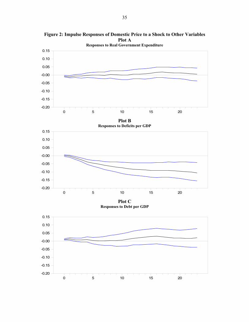
In Figure 2, plots A to I depict the impulse responses of the price level to a shock

in the real government expenditure, deficits per GDP, debt per GDP, foreign-financed

debt per GDP, money supply, domestic interest rate, real exchange rate, real GPP and the

price level, respectively. As we can see all responses are within the confidence band.

Figure 2 about here

Note that all plots in Figure 2 show the normalized responses of a shock. The

normalization has been done by dividing the response by its innovation variance. This

allows all the responses to a shock to be plotted on a single scale. According to Plot (A),

a one standard deviation shock to real government expenditures (equal to 0.24 units)

induces a contemporaneous fall of about 0.005 units in the price level. The fall in price

continues two years before reaching zero at the 9th quarter. Therefore, the impulse is

transitory. According to Plot (B), a one standard deviation shock to deficits per GDP

(equal to 0.0044 units) induces a contemporaneous increase of 0.001 units in the price

level. The price level, then, will fall gradually to -0.06 units at the 24th quarter; therefore,

the impulse response is permanent. Consequently, unanticipated fiscal deficits may have

a deflationary effect in developing countries, or at least in Turkey.

According to Plot (C), a one standard deviation shock to the outstanding debt per

GDP (equal to 0.015 units) induces a contemporaneous increase of 0.008 units in the

price level. The rise in price continues to 0.014 units at the 24th quarter; therefore, the

impulse is permanent. According to Plot (D), one standard deviation shock to foreign

financing per GDP (equal to 0.0016 units) induces a contemporaneous decline of 0.005

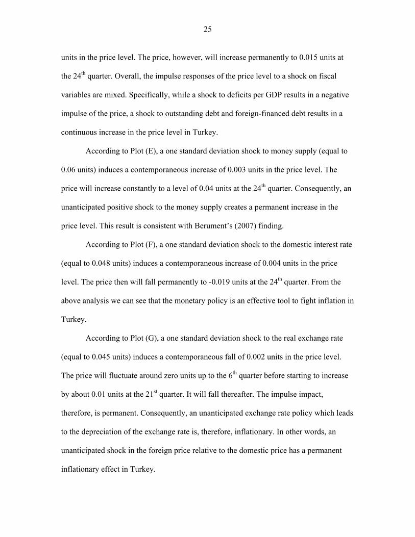
25 units in the price level. The price, however, will increase permanently to 0.015 units at

the 24th quarter. Overall, the impulse responses of the price level to a shock on fiscal

variables are mixed. Specifically, while a shock to deficits per GDP results in a negative

impulse of the price, a shock to outstanding debt and foreign-financed debt results in a

continuous increase in the price level in Turkey.

According to Plot (E), a one standard deviation shock to money supply (equal to

0.06 units) induces a contemporaneous increase of 0.003 units in the price level. The

price will increase constantly to a level of 0.04 units at the 24th quarter. Consequently, an

unanticipated positive shock to the money supply creates a permanent increase in the

price level. This result is consistent with Berument’s (2007) finding.

According to Plot (F), a one standard deviation shock to the domestic interest rate

(equal to 0.048 units) induces a contemporaneous increase of 0.004 units in the price

level. The price then will fall permanently to -0.019 units at the 24th quarter. From the

above analysis we can see that the monetary policy is an effective tool to fight inflation in

Turkey.

According to Plot (G), a one standard deviation shock to the real exchange rate

(equal to 0.045 units) induces a contemporaneous fall of 0.002 units in the price level.

The price will fluctuate around zero units up to the 6th quarter before starting to increase

by about 0.01 units at the 21st quarter. It will fall thereafter. The impulse impact,

therefore, is permanent. Consequently, an unanticipated exchange rate policy which leads

to the depreciation of the exchange rate is, therefore, inflationary. In other words, an

unanticipated shock in the foreign price relative to the domestic price has a permanent

inflationary effect in Turkey.

26

As Plot (H) shows, a one standard deviation shock to the real GDP (equal to 0.045

units) induces a contemporaneous fall of 0.01 units in the price level. The price will

continue to fall permanently to 0.018 units at the 24th quarter. Finally, as Plot (I) shows, a

one standard deviation shock to the price level (equal to 0.031 units) induces permanent

increases in itself. In sum, the most inflationary induced shocks in Turkey are the

outstanding debt and the foreign financing of the debt as well as the positive monetary

policy shocks, i.e., a shock to the money supply or the exchange rate.

We analyze variance decompositions for various time horizons in order to

investigate whether fiscal, monetary and other shocks have played much of a role in

accounting for movements in the price level. Table 4 reports variance decompositions for

various time horizons. Each row shows the fraction of the t-step ahead of forecast error

variance for the price level that is attributed to shocks to the column variables. According

to these results, the real government expenditures, the debt per GDP, the foreign

financing per GDP, the domestic interest rate, the real exchange rate and the real GDP

shocks account for an insignificant percentage of the price forecast error variance at all

horizons. The deficits per GDP and the money supply shocks account for an increasing

percentage of the price forecast error variance as the time horizon increases. This result is

very similar for Iran which operates under an Islamic system, see Kia (2006a).

Table 4 about here

For instance, after four quarters, the deficits per GDP shocks account for 7.60% of

the price forecast error variance. This rises to 31.24% after three years and to 37.14%

after six years. The money supply shocks account for 13.05% after a year, but rises to

15.75% after six years. These results, similar to what was found by Kia, imply that

27 deficits and money supply shocks play a relatively important role in price fluctuations.

However, the major impact of these shocks only occurs with quite a long lag.

Interestingly, opposite to what was found by Kia (2006a) for Iran, more than half of the

price forecast error variance is due to innovations in itself up to two years, but as the error

variance of the deficits and the money supply goes up the price forecast error variance

will fall to about 35%. For example, the price forecast error variance is 63.23% at one

quarter ahead and falls to 50.71% after two years (not reported in the table). It continues

to fall to 35.08% after six years.

VI. Conclusions

Turkey relies heavily on agricultural products and has experienced a period of

both high inflation and public debt. I extended and tested the monetary model of inflation

rate developed by Kia (2006a) on Turkish data, focusing on internal and external factors,

which influence the inflation rate in Turkey. It was found that the monetary policy,

including the foreign exchange policy, is an effective tool to fight inflation in Turkey

over the long run. Specifically, while a tight monetary policy (a higher interest rate)

results in a higher price level over the long run, a weaker currency can help to lower

inflation in Turkey. The former effect also confirms Sargent and Wallace’s view that a

current tight monetary policy leads to a higher inflation rate over the long run.

In Turkey, over the long run, the increase in the real government expenditures

causes the inflation to fall, but the accumulation of debt will raise the inflation rate.

Furthermore, it was found that as debt is financed externally, the demand for the domestic

currency increases and so the price level falls over the long run. In general, it was found

28 the major factors affecting inflation in Turkey over the long run are internal rather than

external factors.

An increase in the interest rate, while over the long run leads to a higher price

level, will reduce the inflation rate over the short run implying a tight monetary policy is

effective only over the short run in Turkey. However, it was found that an unanticipated

shock to the interest rate has a permanent deflationary effect. Interestingly, while increase

in the size of the government, measured by the government expenditures, creates an

inflationary environment over the short run, it leads to a deflationary environment over

the long run. This is possible when a significant part of the government expenditures is

used on infrastructural investment. Furthermore, it was found that an unanticipated shock

to the government expenditures has only a short-run effect in this country. However, an

unanticipated shock to the deficit and the debt per GDP has a permanent effect.

As for the external determinates of inflation in Turkey, it was found that only over

the short run the change in the world interest rate leads to higher inflation. However, an

unanticipated change in the foreign price relative to the domestic price (the real exchange

rate) results in a permanent inflationary effect. The policy regime changes over the

managed exchange rate, similar to the current flexible exchange rate period (since 2001),

had a downward pressure on the short-run dynamics of inflation in Turkey. Another

domestic shock to inflation was found to be the financial crisis of 1994 which resulted in

a higher inflation rate. The overall conclusion is that the sources of inflation in Turkey

are mainly internal factors. They arise mostly from the monetary policy.

29

References

Arize, Augustine C., John Malindretos and Srinivas Nippani (2004), “Variations in

Exchange Rates and Inflation in 82 Countries: An Empirical Investigation”, The

North American Journal of Economics And Finance, 15, 227-247.

Ashra, Sunil, Saumen Chattopadhyay and Kausik Chaudhuri (2004), “Deficit, Money and

Price: the Indian Experience”, Journal of Policy Modeling, 26, 289-299.

Bahmani-Oskooee, Mohsen (1995), “Source of Inflation in Post-Revolutionary Iran”,

International Economic Journal, 9, 2, summer, 61-72.

Baydur, Cem Mehmet and Bora Süslü (2004), “The View of Sargent and Wallace on

Monetary Policy: Tight Monetary Policy Does not Stop Inflation: an Evaluation

of CBRT’s Monetary Policy for 1987-2002”, Journal of Policy Modeling, 26,

191-208.

Berument, Hakan and Zubeyir Kilinc (2004), “The Effect of Foreign Income on

Economic Performance of a Small-Open Economy: Evidence from Turkey”,

Applied Economics Letters, 11, 483-488.

Berument, Hakan (2007), “Measuring Monetary Policy for a Small Open Economy:

Turkey”, Journal of Macroeconomics, 29, 411-430.

Boschi, Melisso and Alessandro Girardi (2007), “Euro Area Inflation: Long-run

Determinants and Short-Run Dynamics”, Applied Financial Economics, 17, 9-24.

Cheung, Y. and K.S. Lai (1993), “Finite-sample Sizes of Johansen’s Likelihood Ratio

Tests for Cointegration”, Oxford Bulletin of Economics and Statistics, 55,

313-328.

Dennis, Jonathan G. (2006), CATS in RATS, Version 2, Evanston, Estima.

30 Dornbusch, Rudiger, Sturzenegger, Fedrico, Wolf, Holger, Fischer, Stanley and Robert

Barro (1990), “Extreme Inflation: Dynamics and Stabilization”, Brookings Papers

on Economic Activity, 1990, 2, 1-84.

Drazen, Allan and Elhanan Helpman (1990), “Inflationary Consequences of Anticipated

Policies”, The Review of Economics Studies, 57, 1, January, 147-164.

El-Sakka, M. I. T. and Khalifa H. Ghali (2005), “The Sources of Inflation in Egypt: A

Multivariate Co-integration Analysis”, Review of Middle East Economics and

Finance, 3, 3, 257-269.

Engle, Robert F. (1982), “Autoregressive Conditional Heteroskedasticity With Estimates

of the Variance of United Kingdom Inflation”, Econometrica, July, 987-1007.

Engle, Robert F., David F. Hendry and Jean-François Richard (1983), “Exogeneity”,

Econometrica, 51, 2, March, 277-304.

Engle, Robert F. and David F. Hendry (1993), “Testing Superexogeneity and Invariance

in Regression Models”, Journal of Econometrics, 56, 119-139.

Godfrey, Les G. (1978), “Testing Against General Autoregressive And Moving Average

Error Models When the Regressors Include Lagged Dependent Variables”,

Econometrica, November, 1293-1301.

Godfrey, Les G. (1988), Misspecification Tests in Econometrics, New York, Cambridge

University Press.

Granger, Clive W.J. (1986), “Developments in the Study of Cointegrated Economic

Variables”, Oxford Bulletin of Economics and Statistics, August, 213-218.

Hansen, Bruce E. (1992), “Testing for Parameter Instability in Linear Models”, Journal

of Political Modeling, 14, 4, 517-533.

31 Hansen, Henrik and Katarina Juselius (1995), CATS in RATS Cointegration Analysis of

Time Series, Evanston, Estima.

Jarque, Carlos M. and Anil K. Bera (1987), “A Test for Normality of Observations and

Regression Residuals”, International Statistical Review, 55, 2, August, 163-172.

Johansen, Soren (1995), Likelihood-Based Inference in Cointegrated Vector

Autoregressive Models, Oxford, Oxford University Press.

Johansen, Soren and Katarina Juselius (1991), “Testing Structural Hypotheses in a

Multivariate Cointegration Analysis of the PPP and the UIP for UK”, Journal of

Econometrics, 53, 211-244.

Johansen, Soren and Katarina Juselius (1994), “Identification of the Long-Run and the

Short-Run Structure: An Application to the ISLM Model”, Journal of

Econometrics, 63, 7-36.

Kia, Amir (2003a), “Forward-Looking Agents and Macroeconomic Determinants of the

Equity Price in a Small Open Economy”, Applied Financial Economics, 13,

37-154.

Kia, Amir (2003b), “Rational Speculators and Equity Volatility as a Measure of Ex Ante

Risk”, Global Finance Journal, 14, 135-157.

Kia, Amir (2006a), “Deficits, Debt Financing, Monetary Policy and Inflation in

Developing Countries: Internal or External Factors? Evidence from Iran”, Journal

of Asian Economics, 17, 879-903.

Kia, Amir (2006b), “Economic Policies and Demand for Money: Evidence from

Canada”, Applied Economics, 38, 1389-1407.

32 Lim, Cheng Hoon and Laura Papi (1997), “An Econometric Analysis of the Determinants

of Inflation in Turkey”, International Monetary Fund, WP/97/170.

Lütkepohl, Helmut and Hans-Eggert Reimers (1992), “Impulse Response Analysis of

Cointegrated Systems”, Journal of Economics Dynamics and Control, 16, 53-78.

The Middle East and North Africa (2004), London, Europa Publications.

Özatay, Faith (1997), “Sustainability of Fiscal Deficits, Monetary Policy, and Inflation

Stabilization: The Case of Turkey”, Journal of Policy Modeling, 19, No. 6,

661-681.

Pagan, Adrian (1984), Econometric Issues in the Analysis of Regressions with Generated

Regressors, International Economic Review, February, 221-247.

Pongsaparn, Runchana (2002), “Inflation Dynamics and Reaction Function in

High-Inflation Environment: An Implication for Turkey”, The Central Bank of the

Republic of Turkey, Research Department Working Paper No. 10.

Rabanal, Pau (2007), “Does Inflation Increase After a Monetary Policy Tightening?

Answers Based on an Estimated DSGE Model”, Journal of Economic Dynamics

and Control, 31, 906-937.

Ramsey, J.B. (1969), “Tests for Specification Errors in Classical Linear Least-squares

Regression Analysis”, Journal of Royal Statistical Society, Series B, 31, 2,

350-371.

Sargent, Thomas J. and Neil Wallace (1986), “Some Unpleasant Monetarist Arithmetic”,

Chapter 5 in Sargent, Thomas, Rational Expectations and Inflation, New York,

Harper & Row Publisher.

33 Schmidt, Peter and Peter C. B. Phillips (1992), "LM Test for a Unit Root in the Presence

of Deterministic Trends", Oxford Bulletin of Economics and Statistics, 54, 3,

257-287.

Stock, J.H., and M.W. Watson (1993), “Interpreting the Evidence on Money-Income

Causality,” Journal of Econometrics, 40, 161-182.

Tawadros, George B. (2007), “Testing the Hypothesis of Long-run Money Neutrality in

the Middle East”, Journal of Economic Studies, 34, 1, 13-28.

Tekin-Koru, Ayca and Erdal Ozmen (2003), “Budget Deficit, Money Growth and

Inflation: the Turkish Evidence”, Applied Economics, 35, 591-596.

Telli, Cagatay, Voyvoda, Ebru and Erinc Yeldan (2008), “Macroeconomics of

Twin-targeting in Turkey: Analytics of a Financial Computable General

Equilibrium Model”, International Review of Applied Economics, 22, 2, 227-242.

Togan, Sübidey (1987), “The Influence of Money and the Rate of Interest on the Rate of

Inflation in a Financially Repressed Economy: the Case of Turkey”, Applied

Economics, 19, 1585-1601.

Us, Vuslat (2004), “Inflation Dynamics and Monetary Policy Strategy: Some Prospects

for the Turkish Economy”, Journal of Policy Modeling, 26, 1003-1013.

White, Halbert (1980), “A Heteroskedasticity-Consistent Covariance Matrix Estimator

and a Direct Test for Heteroskedasticity”, Econometrica, May, 817-837.

Williams, Oral H. and Olumuyiwa S. Adedeji (2007), “Inflation Dynamics in a Small

Emerging Market”, Applied Economics, 39, 407-414.

34

Figure 1: Recursive Likelihood Ratio Tests

Test of known beta eq. to beta(t)

1 is the 5% significance level1997 1998 1999 2000 2001 2002 2003

0.0

0.8

1.6

2.4

3.2

4.0

4.8

5.6 BETA_ZBETA_R

35

Figure 2: Impulse Responses of Domestic Price to a Shock to Other Variables Plot A

Responses to Real Government Expenditure

0 5 10 15 20-0.20

-0.15

-0.10

-0.05

-0.00

0.05

0.10

0.15

Plot B

Responses to Deficits per GDP

0 5 10 15 20-0.20

-0.15

-0.10

-0.05

-0.00

0.05

0.10

0.15

Plot C

Responses to Debt per GDP

0 5 10 15 20-0.20

-0.15

-0.10

-0.05

-0.00

0.05

0.10

0.15

36

Figure 2 Continues Plot D

Responses to Foreign-Financed Debt Per GDP

0 5 10 15 20-0.20

-0.15

-0.10

-0.05

-0.00

0.05

0.10

0.15

Plot E

Responses to Real M1

0 5 10 15 20-0.20

-0.15

-0.10

-0.05

-0.00

0.05

0.10

0.15

Plot F

Responses to Domestic Interest Rate

0 5 10 15 20-0.20

-0.15

-0.10

-0.05

-0.00

0.05

0.10

0.15

37

Figure 2 Continues Plot G

Responses to Real Exchange Rate

0 5 10 15 20-0.20

-0.15

-0.10

-0.05

-0.00

0.05

0.10

0.15

Plot H

Responses to Real GDP

0 5 10 15 20-0.20

-0.15

-0.10

-0.05

-0.00

0.05

0.10

0.15

Plot I

Responses to the Price Level

0 5 10 15 20-0.20

-0.15

-0.10

-0.05

-0.00

0.05

0.10

0.15

38

Table 1*: Long-Run Test Results Tests of the Cointegration Rank

H0= r 0 1 2 3 4 5 6 7 8 Diagnostic tests**

p-value

Trace(1) 272.70 191.24a 135.88 85.29 60.54 48.24 22.93 11.40 3.08 Test for Autocorrelation: LM(5)** 0.41

Trace 95(2) 257.48 214.59 176.30 141.06 109.89 81.44 57.01 35.47 19.19 Test for ARCH: LM(1)** 0.10 LM(2) ** 0.01 Test for Normality: χ2= 178 0.00 Lag length = 5

Test for the Restricted Long-Run Relationship. Restrictions are accepted: χ2 (1) = 4.95, p-value = 0.03 Normalized lp lMs i ly lq i* lg defgdp debtgdp fdgdp constant

lp (t-statistic)

- Rest.

= 1.00

1.19

(6.89)

0.33

(1.37)

-3.32

(-7.76)

0.04

(0.37)

-1.55

(-8.25)

0.13

(0.09)

1.44

(2.83)

-66.00

(-9.55)

47.14

(7.81)

Stock and Watson’s (1993) Dynamic OLS Results*** Wald statistic = 108.38 (p-value=0.00)

lp (t-statistic)

- Rest.

= 1.00

0.44

(5.07)

-0.79

(-4.76)

-0.23

(-0.88)

-0.22

(-4.46)

0.14

(1.05)

2.48

(3.01)

1.09

(4.03)

-7.38

(-1.99)

3.54

(0.96)

a = accept the null of r=1. (1) The Trace test has been multiplied by the small sample correction factor (N – kp)/N, see Cheung and Lai (1993). (2) CATS 2 in RATS computer package was used to simulate the critical values. The number of replications was 2500 with a length of random walks of 400. * The sample period is 1970Q1-2003Q3. lMs is the log of nominal money supply, i and i* are the log[R/(1+R)]and log[R*/(1+R*)], respectively, where R and R* are domestic and foreign interest rates in decimal points, respectively, ly is the log of the real GDP, lq is the log of the real exchange rate, lp is the log of domestic CPI, lg is the log of the real government expenditures on goods and services, defgdp and debtgdp are deficits and outstanding debt per GDP, respectively, and fdgdp is the amount of the foreign-financed debt per GDP. ** LM(i), for i=1, 2 and 5, is ith-order Lagrangian Multiplier test for autocorrelation, respectively [Godfrey (1988)]. *** Stock and Watson’s (1993) test (DOLS) is based on the following regression: lpt = β0 + lMst + β2 it + β3 lyt + β4 lqt + β5 i*t + β6 lgt + β7 defgdpt + β8 debtgdpt + β9 fdgdpt + δ1(L) ∆lMst + δ2(L) ∆it + δ3(L) ∆lyt + δ4(L) ∆lqt + δ5(L) ∆i*t + δ6(L) ∆lgt + δ7(L) ∆defgdpt + δ8(L) ∆debtgdpt +δ9(L) ∆fdgdpt + DUMt’ α + ut,, where δi(L), for i=1 and 2, has two leads and lags.

39

Table 2*: Error Correction Model for the Inflation Rate Structural Form

Dependent Variable Δlp

Independent

Variables

Coefficients Standard Error

Hansen ’s (1992) Li stability test p-value

Constant -0.16 0.05 0.42

Δlyt -0.31 0.09 0.63

Δit-3 -0.02 0.01 0.25

Δi*t-2 0.06 0.03 0.12

Δlyt-1 0.22 0.05 0.64

(ECP)2t-2 0.06 0.03 0.11

(ECP)3t-2 -0.04 0.02 0.85

Δlp-1 0.21 0.08 0.83

Δlp-2 -0.14 0.06 0.43

fcrisis 0.17 0.03 0.14

flex -0.07 0.02 0.97

pex -0.07 0.02 1.00

Trend 0.001 0.0002 0.46

Nor1980Q1Q2 0.14 0.03 1.00

Nor 1988Q1 0.13 0.03 0.04

Li test on variance p-value = 0.35 Joint Lc test*** p-value = 0.41 R 2=0.70, σ=0.03, DW=1.66, Godfrey(5)=1.34 (significance level=0.24), White=0.99 (significance level=0.99), ARCH(5)=9.75 (significance level=0.08), RESET=0.21 (significance level=0.89) and Normality, Jarque-Bera = 4.34 (significance level=0.11).

* The estimation method is the Ordinary Least Squared. The sample period is 1970Q1-2003Q3. Δ means the first difference, Δlp is the change in the log of CPI and Δly is the change in the log of the real GDP. Δi and Δi* are, respectively, the change in the log[R/(1+R)] and log[R*/(1+R*)], where R and R* are, respectively, the nominal domestic and foreign interest rates in decimal points. ECP is the error-correction term. Dummy variable fcrisis is equal to 1 for 1994Q2 and to zero, otherwise. Dummy variable flex is equal to 1 since 2001Q1 and to zero, otherwise. Dummy variable pex is equal to 1 for the period of 2000Q1-2000Q4 and to zero, otherwise. Trend is a linear time trend. Nor1980Q1Q2 is equal to 1 during the first and second quarters of 1980, and to zero, otherwise, and Nor 1988Q1 is equal to 1 in the first quarter of 1988, and to zero, otherwise. These dummy variables were used to eliminate the outliers in the data.

40

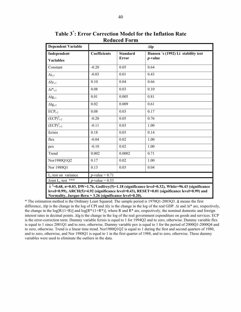
Table 3*: Error Correction Model for the Inflation Rate Reduced Form

Dependent Variable Δlp

Independent

Variables

Coefficients Standard Error

Hansen ’s (1992) Li stability test p-value

Constant -0.20 0.05 0.64

Δit-3 -0.03 0.01 0.43

Δlyt-1 0.10 0.04 0.66

Δi*t-2 0.08 0.03 0.10

Δlgt-1 0.01 0.005 0.81

Δlgt-2 0.02 0.009 0.61

ECPt-2 0.08 0.03 0.17

(ECP)2t-2 -0.20 0.05 0.76

(ECP)3t-2 -0.11 0.03 1.00

fcrisis 0.18 0.03 0.14

flex -0.04 0.02 1.00

pex -0.10 0.02 1.00

Trend 0.002 0.0002 0.71

Nor1980Q1Q2 0.17 0.02 1.00

Nor 1988Q1 0.13 0.03 0.04

Li test on variance p-value = 0.71 Joint Lc test *** p-value = 0.53 R 2=0.68, σ=0.03, DW=1.76, Godfrey(5)=1.18 (significance level=0.32), White=96.43 (significance level=0.99), ARCH(5)=4.92 (significance level=0.43), RESET=0.01 (significance level=0.99) and Normality, Jarque-Bera = 3.26 (significance level=0.20).

* The estimation method is the Ordinary Least Squared. The sample period is 1970Q1-2003Q3. Δ means the first difference, Δlp is the change in the log of CPI and Δly is the change in the log of the real GDP. Δi and Δi* are, respectively, the change in the log[R/(1+R)] and log[R*/(1+R*)], where R and R* are, respectively, the nominal domestic and foreign interest rates in decimal points. Δlg is the change in the log of the real government expenditure on goods and services. ECP is the error-correction term. Dummy variable fcrisis is equal to 1 for 1994Q2 and to zero, otherwise. Dummy variable flex is equal to 1 since 2001Q1 and to zero, otherwise. Dummy variable pex is equal to 1 for the period of 2000Q1-2000Q4 and to zero, otherwise. Trend is a linear time trend. Nor1980Q1Q2 is equal to 1 during the first and second quarters of 1980, and to zero, otherwise, and Nor 1988Q1 is equal to 1 in the first quarter of 1988, and to zero, otherwise. These dummy variables were used to eliminate the outliers in the data.

41

Table 4* Price Level Variance Decompositions Shock to: Period (Quarters)

lg defgdp debtgdp fdgdp lMs i lq ly lp

1 4.33 0.10 9.96 3.17 0.95 1.97 0.58 15.72 63.23 4 2.73 7.60 4.21 1.39 13.05 0.98 0.52 7.63 61.89 12 0.36 31.24 0.93 0.97 14.76 3.03 0.25 5.35 43.12 20 0.56 36.43 2.76 0.89 15.62 3.18 0.36 4.18 36.02 24 0.48 37.14 2.56 1.18 15.75 3.34 0.47 4.01 35.08

* See footnote of Table 1 for the mnemonics.