Student

Spring 2014

Master thesis I, 15 ECTS

Master’s program in Economics, 60/120 ECTS Supervisor: Christian Lundström

Money Management Using the Kelly Criterion

An Application of the Kelly Criterion on an Intraday Trading Strategy Based on the Swedish Stock Market Index OMXS30

Mårten Hagman

Abstract

This paper highlights the importance of money management. Firstly, we show how an

intraday trading strategy based on Swedish stock market index OMXS30 can be developed

given market ineffectiveness. Secondly, we maximize the profitability of this technical trading

strategy by applying the Kelly money management criterion. We estimate a concave

relationship to find the optimal leverage factor. The main finding is that the profitability can

be increased substantially for the given trading strategy.

Key words: Breakout filter, Day trading, Future contracts, Kelly criterion, Market

inefficiency, Money management, Optimal leverage factor, Relative strength index

Acknowledgements

I would like to thank my study companions for the support and the great company, enabling

me to get through the long days of studies. I would also like to express my big gratitude

towards Christian Lundström for all the inspiration he has given me and also for guiding me,

with his expertise, through the financial jungle.

Table of content

1. Introduction ......................................................................................................................................... 1

1.1 Background ................................................................................................................................... 1

1.2 Structure ........................................................................................................................................ 3

2. Money management ............................................................................................................................ 3

2.1 Previous studies ............................................................................................................................. 3

2.2 The Kelly criterion ........................................................................................................................ 5

2.3 Application of Kelly criterion on future contracts......................................................................... 8

3. Technical analysis ............................................................................................................................... 9

3.1 The efficient market hypothesis .................................................................................................... 9

3.2 RSI ............................................................................................................................................... 11

3.3 Daily breakout filter .................................................................................................................... 11

3.4 The trading strategy ..................................................................................................................... 12

4. Empirical results ................................................................................................................................ 14

4.1 Data ............................................................................................................................................. 14

4.2 Profitability test ........................................................................................................................... 15

4.2.1 Model.................................................................................................................................... 15

4.2.2 Results .................................................................................................................................. 16

4.3 Applying the Kelly criterion on the trading strategy ................................................................... 18

4.4 Comparing the optimized θ to θ=1 .............................................................................................. 19

4.5 Using a high leverage factor ........................................................................................................ 20

4.6 Test of robustness ........................................................................................................................ 21

4.7 Overview of results from the test period ..................................................................................... 23

5. Conclusions ....................................................................................................................................... 23

References ............................................................................................................................................. 25

Appendix ............................................................................................................................................... 28

A. How to practically obtain θ ....................................................................................................... 28

B. Relative strength index .............................................................................................................. 29

C. Frequency histogram of returns .................................................................................................. 30

1

1. Introduction

1.1 Background

What do a risk neutral gambler and an investor have in common? Both want to make as much

money as possible. By using money management this paper shows how the capital or wealth

of an investor can be maximized. Money management can, as we partly will demonstrate, be

seen as a field that in many aspects ties gambling theory together with financial theory. The

main goal of money management is to maximize the capital growth by applying an optimal

leverage factor without risk of ruin. We define the concept of ruin as substantial losses of

capital that limits the amount we can reinvest. If ruin occurs it thereby causes a constraint in

possible capital growth. In his paper we test the theory Kelly criterion. This theory is

suggested by many high achieving investors as a way to handle the money management.

Among these investors we find John Maynard Keynes, Warren Buffet and Bill Gross

(Lundström, 2014).

The contribution of this paper to the field of money management is the application of Kelly

criterion on an intraday trading strategy based on the Swedish stock market index OMXS30. 1

By involving money management when studying a trading strategy we highlight a flaw of

many similar studies. What can be noticed when observing previous studies of investment

strategies is that they are often simplified. Many studies are limited to investing the same

amount for every trade and not allowing for reinvestments (e.g. Wang and Yu, 2000). In this

study we allow for reinvestments of capital gains and thereby, unlike earlier simplified

studies, we present a more reality based study. Using reinvestments, the capital grows or

shrinks at an exponential speed (Kelly, 1956).

Given that an agent is utility maximizing and risk neutral, it should be of importance that we

maximize the profit in the long run without risk of ruin.2 Under the assumption that one

possesses an investment strategy that generates a positive average return, determining the size

1 The index corresponds to the 30 most traded stocks listed on the Stockholm stock exchange, corresponding to

65% of the trading volume and 45% of the market value. 2 Risk of ruin can be defined as the probability of losing sufficient trading or gambling money to the point where

continuing a trading strategy or game is no longer considered an option to recover losses.

2

of the investment is essential. It can analogously be seen as a bet size decision of a blackjack

player who is exploiting an edge he or she has in the game (Anderson and Faff, 2004).

To practically perform a strategy like the one we present in this paper a financial instrument is

needed. Future contracts are a financial instrument that well suits for active trading. There are

a several reasons why future contracts are a facilitating instrument for this study. At first

trading futures is very common and frequently used for agents acting on the financial markets.

For instance, trading futures is a multi-billion US dollar industry (Lundström, 2014). Some

primary reasons behind the wide prevalence are the low transaction costs and the liquid

market of futures. Future contracts do also have the advantage that it is just as easy to make

long trades as short trades. Its flexibility to make long and short trades also offers an

opportunity for people who want to hedge against risk. Moreover, future contracts also offer

the investor to set their own risk by allowing for different leverage factors.

When trading futures, determining the investment size can equally be seen as determining

what leverage factor to use (Sewell, 2011). When referring to investment size when observing

future contracts, we from now on refer to it as leverage factor and denote it by the Greek letter

. Thus, setting is the same as not involving money management. By being able to

adjust the leverage factor without any additional transaction costs, futures offer a great

flexibility. For an example of how is obtained practically, see appendix A. Since we have

chosen to use future contracts of OMXS30 we now need a trading strategy that gives us

empirical returns and a way to determine the optimal leverage factor. The optimal leverage

factor is the one which gives us the highest growth rate of capital. The method of optimizing

is the Kelly criterion and is explained in chapter 2.

The trading strategy that is used as a base for the Kelly criterion is applied on futures traded

on an intraday basis; meaning that we buy and sell the future contract the same day. Trading

strategies applied for future contracts on intraday basis has earlier been proven successful by

Holmberg et al. (2013) and Lundström (2013). Both studies base their trading strategies on

intraday momentum in price movements. Important to clarify is that strategies like Holmberg

et al. (2013), Lundström (2013) and the one used for this paper rely on the assumption of

market ineffectiveness. The concept market ineffectiveness is explained in chapter 3.

The trading strategy we use involves two tools in technical analysis, the relative strength

index (RSI) and a breakout filter. The RSI was developed by Wilder (1978) and has a huge

advantage that it is developed during a time when data snooping was not possible. Data

3

snooping refers to testing multiple trading tools at the same time and just present the tools

producing profits. This has the implication that the tools showing profitable return might be

random (Sullivan et al, 1999). The breakout filter has the benefit of capturing momentum in

price developments. These trading tools are more closely explained in section 3.2 and 3.3.

The main purpose of this paper is to study whether it is possible to optimize an already

profitable day trading strategy by applying the Kelly criterion. The paper also aims to prove

the consequences of being too aggressive or too timid when investing. To avoid the study of

becoming too complex we have limited the study as follows. At first, there are many aspects

of optimizing a trading strategy; hence we limit the study by just applying the Kelly criterion

for one type of trade (long trades) for the given strategy. Secondly, compared to other studies

we just apply it on one type of future contract (OMXS30 futures). Thirdly, we do also not

consider the aspect of stop losses when we trade; the use of stop losses is briefly explained in

section 2.1.

1.2 Structure

This paper can be seen as a two parts study. The first part concerns the investment strategy

and the second part is the optimization of that strategy through Kelly criterion. The outline of

the remaining parts of the paper is as follows. Chapter 2 presents some of the earlier studies of

applications of the Kelly criterion and also clarifies more in depth what the Kelly criterion is

and how it works. Chapter 3 presents some concepts about the nature of financial markets, the

technical trading tools and the strategy used for this paper. Further, Chapter 4 shows the

empirical results by containing a profitability test of the investment strategy and later the

solution to the optimization problem through the Kelly criterion. Finally, Chapter 5 sums up

the paper in a concluding discussion.

2. Money management

2.1 Previous studies

Kelly (1956) shed new light to gambling theory by showing that when reinvesting the capital

one includes the aspect of money growing or shrinking at an exponential rate. In that way

Kelly’s sort of thinking differs from the classical gambling theory. Kelly presented his

criterion through a lottery with positive expected value and two outcomes (we present a

similar example in section 2.2) where the capital gains is reinvested. Thorp (1969) developed

Kelly’s original gambling strategy by expanding it to several Casino games such as

4

Blackjack, Baccarat, Roulette and Wheel of fortune. Further, Thorp (1969) also suggested the

application of the Kelly criterion to the stock market and financial derivatives by using a

continuous probability distribution of the returns instead of the discrete distribution of Kelly’s

original lottery example. However, Thorp (1969) assumed that the distribution of returns

followed a log normal distribution, which can be questioned when applying it to the stock

market. For instance Cont (2001) shows that financial returns follow a distribution with heavy

tales. This would imply that Thorp (1969) underestimated the risk by using a log normal

distribution.

After Thorp (1969) widened the use of Kelly criterion it has been suggested by a several

authors during the years. Gehm (1983) applied the Kelly criterion to the commodity market

when trading futures and later on also Balsara (1992) used the Kelly criterion for the same

purpose. Rotando and Thorp (1992) showed it was possible to apply the Kelly criterion on the

SAP500 index. Rotando and Thorp (1992) divided the period between the years 1926-1984

into one year intervals and optimized the investment size over the time period based on the

average return of 5.8% per annum. The findings of Rotando and Thorp (1992) suggest that

one should invest 117% of the capital each year, hence borrow 17% additional capital to

invest each year. However, the result of Rotando and Thorp (1992) was not corrected for

transaction costs.

Further, Tharp (1997) uses the Kelly criterion to highlight the importance of money

management rather than looking for trading strategies which aim to find the right time to enter

and exit the market. Vince (1990) develops the Kelly criterion by correcting the optimization

problem for risk. Vince (1990) states, that the optimal bet fraction ( ) should be corrected for

the largest loss in a series of returns. According to Vince the optimal leverage factor (Vince

criterion) should be described as the optimal fraction divided by the largest loss. Andersson

and Faff (2004) use the optimal -technique like Vince (1990) for speculative future

contracts. One of the key findings of Andersson and Faff (2004) is the importance of

reinvesting when evaluating the returns for future traders. They highlight reinvestments both

in the sense that it is the scenario in real investment situations and also by showing increased

returns. For instance they achieve an impressive return of 2000% when trading corn futures.

However, according to Andersson and Faff (2004), the Kelly criterion was not able to turn a

losing strategy into profit.

5

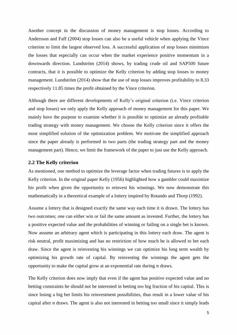
Another concept in the discussion of money management is stop losses. According to

Andersson and Faff (2004) stop losses can also be a useful vehicle when applying the Vince

criterion to limit the largest observed loss. A successful application of stop losses minimizes

the losses that especially can occur when the market experience positive momentum in a

downwards direction. Lundström (2014) shows, by trading crude oil and SAP500 future

contracts, that it is possible to optimize the Kelly criterion by adding stop losses to money

management. Lundström (2014) show that the use of stop losses improves profitability to 8.33

respectively 11.85 times the profit obtained by the Vince criterion.

Although there are different developments of Kelly’s original criterion (i.e. Vince criterion

and stop losses) we only apply the Kelly approach of money management for this paper. We

mainly have the purpose to examine whether it is possible to optimize an already profitable

trading strategy with money management. We choose the Kelly criterion since it offers the

most simplified solution of the optimization problem. We motivate the simplified approach

since the paper already is performed in two parts (the trading strategy part and the money

management part). Hence, we limit the framework of the paper to just use the Kelly approach.

2.2 The Kelly criterion

As mentioned, one method to optimize the leverage factor when trading futures is to apply the

Kelly criterion. In the original paper Kelly (1956) highlighted how a gambler could maximize

his profit when given the opportunity to reinvest his winnings. We now demonstrate this

mathematically in a theoretical example of a lottery inspired by Rotando and Thorp (1992).

Assume a lottery that is designed exactly the same way each time it is drawn. The lottery has

two outcomes; one can either win or fail the same amount as invested. Further, the lottery has

a positive expected value and the probabilities of winning or failing on a single bet is known.

Now assume an arbitrary agent which is participating in this lottery each draw. The agent is

risk neutral, profit maximizing and has no restriction of how much he is allowed to bet each

draw. Since the agent is reinvesting his winnings we can optimize his long term wealth by

optimizing his growth rate of capital. By reinvesting the winnings the agent gets the

opportunity to make the capital grow at an exponential rate during draws.

The Kelly criterion does now imply that even if the agent has positive expected value and no

betting constraints he should not be interested in betting too big fraction of his capital. This is

since losing a big bet limits his reinvestment possibilities, thus result in a lower value of his

capital after draws. The agent is also not interested in betting too small since it simply leads

6

to small winnings (Kelly 1956). The problem the agent is facing can be solved by applying

the Kelly criterion, which tells him what fraction of his capital he should bet each time to

optimize the expected value of his wealth after games.

Since the agent is allowed to bet as much as he wants we describe his bet size as a fraction of

his capital, denoted by . Further, if the initial wealth of the agent is denoted as his wealth

after a number of bets ( ), can be described by the following equation:

In the equation above corresponds to the number of successful bets and number of bets

that fails where: .

We follow Kelly (1956), and set the probability of going broke equal to zero by defining the

bet fraction as: . The total growth of wealth after bets can be described as:

The agent is interested in finding the fraction that optimizes the expected growth rate per trial

, i.e. geometric mean. We therefore raise the equation by 1 divided by number of trials

and describe growth rate per trial as follows:

In next step the logarithms used on the function and also expectations. 3

This permits us to

describe and rewrite the expected growth rate per trial in the following manner:

We can denote the expected probability of success and fail as follows:

3 The use of logarithm facilitates for solving the optimization problem.

7

Since it is a binomial lottery with a positive expected value it follows that , where

. Substituting and into the expression now allows us to describe the expected

growth rate as:

The agent is looking to optimize the expected growth rate per trial, hence we take the

derivative with respect to the fraction, .

Recall that . This results in:

In order to confirm that the solution to the optimization problem gives us a maximum of

we show that:

Under the assumption that we have a maximum of growth rate of wealth

when . By applying the Kelly criterion the agent can optimize his expected growth rate

of wealth by betting the following each lottery game:

where is the percentage of the capital which gives the highest expected growth rate.

By using the assumptions in the example we show in figure 1 how different values of

probability of success gives different concave relationships with maximums that are implying

that the higher value of w the bigger fraction of our wealth should be played in each game.

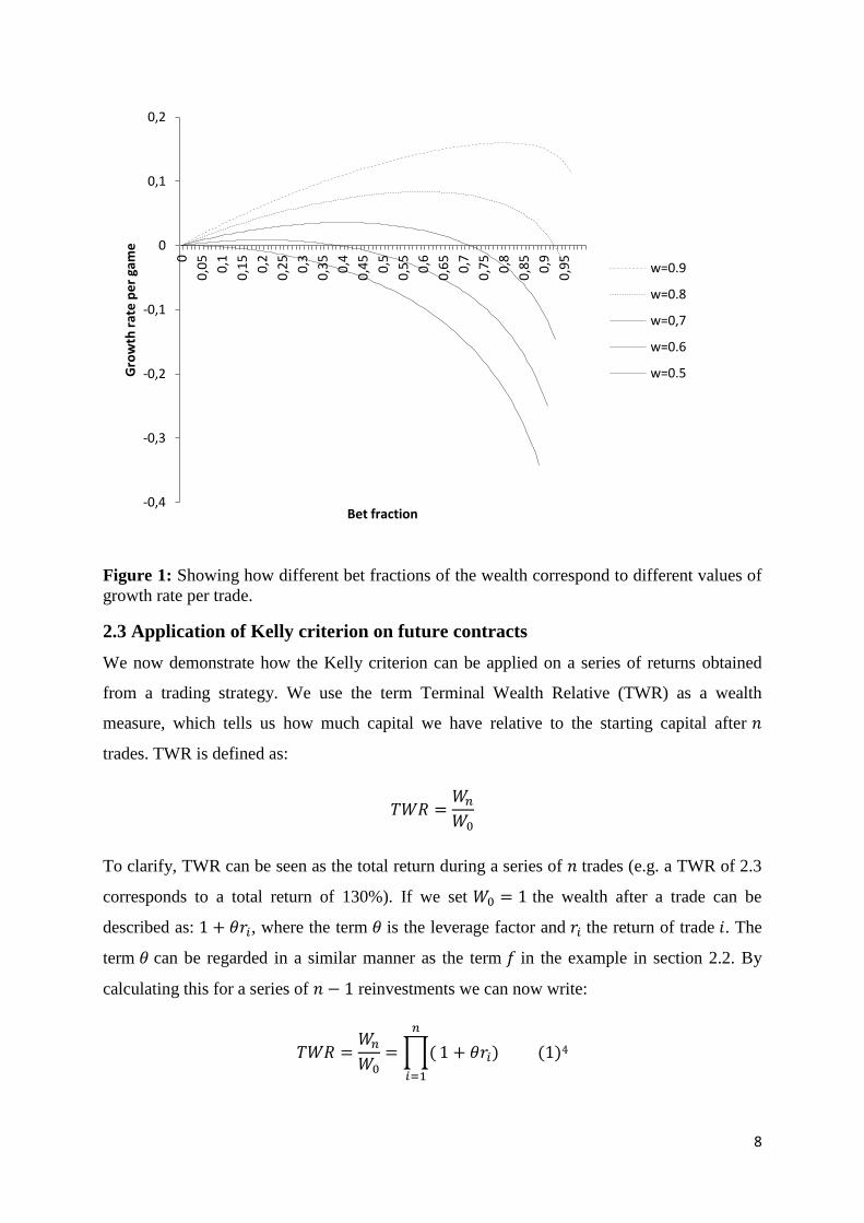
8

Figure 1: Showing how different bet fractions of the wealth correspond to different values of

growth rate per trade.

2.3 Application of Kelly criterion on future contracts

We now demonstrate how the Kelly criterion can be applied on a series of returns obtained

from a trading strategy. We use the term Terminal Wealth Relative (TWR) as a wealth

measure, which tells us how much capital we have relative to the starting capital after

trades. TWR is defined as:

To clarify, TWR can be seen as the total return during a series of trades (e.g. a TWR of 2.3

corresponds to a total return of 130%). If we set the wealth after a trade can be

described as: , where the term is the leverage factor and the return of trade . The

term can be regarded in a similar manner as the term in the example in section 2.2. By

calculating this for a series of reinvestments we can now write:

4

-0,4

-0,3

-0,2

-0,1

0

0,1

0,2

0

0,0

5

0,1

0,1

5

0,2

0,2

5

0,3

0,3

5

0,4

0,4

5

0,5

0,5

5

0,6

0,6

5

0,7

0,7

5

0,8

0,8

5

0,9

0,9

5

Gro

wth

rat

e p

er

gam

e

Bet fraction

w=0.9

w=0.8

w=0,7

w=0.6

w=0.5

9

Like the case for the agent in section 2.2 we are looking for the growth rate per trade (i.e. the

geometric mean):

By taking the logarithm of the expression we can express the growth rate per trade in a

series of successive trades as:

5

To empirically find the optimized we need to obtain empirical values of a series of

returns . To make the study applicable on reality we will divide the time

period into two parts; the first period will be used to obtain the optimal value of that

maximizes the growth rate per trade and then apply that leverage factor on the second part of

the sample. We need to do this since it is not reasonable that we know the optimal in

advance, thus we use the first part to just observe the behavior of the returns and the second

part of the returns to use the optimized obtained from the first part to perform the trading

strategy practically.

3. Technical analysis

3.1 The efficient market hypothesis

Eugene Fama (1965) developed the Efficient Market Hypotheses (EMH). According to EMH

all information are available to the investors. Thereby every financial asset has its correct

price which also is referred to as the equilibrium price. Assuming that all investors act rational

on available information of already happened events, but also events that can be expected in

the future everything is included in the current market price. Given that all information about

that underlying asset is known and used correctly by the investors, it is exactly 50% for

additional information to be either good or bad. Further, under EMH, all agents on the market

are always trying to find systematical patterns in the price development and take advantage of

these. This leads to prices randomly moves around the equilibrium price. Under the

4

5

10

assumption that the prices of financial assets behave as described by EMH, price movement

of these assets can be described as a random walk.

However, there are studies and theories that contradict EMH. Shiller (2001) explains various

biases among investors causing that the market price can often deviate significantly from its

equilibrium price. For instance, representative heuristics is a phenomenon when people tend

to overreact to news resulting that the price deviates from the long term trend due to good or

bad news and then slowly adjust back to its equilibrium price. Further, Shiller also states that

people often seem to neglect history; leading to that people continues to make wrong choices

of investment by not learning from the past. Besides this, Shiller means that some investors in

general believe that they possess magical or quasi magical thinking. These investors are

experiencing that a certain behavior leads to profit but in fact the profit from the “magical”

thinking investors is due to the stochastic nature of financial market or a general economic

growth during the period they performs that certain strategy.

Important to know is that even if Shiller describes a lot of concepts in behavioral finance that

can imply market ineffectiveness he states that relevance of these concepts should be taken

with caution due to the complexity of human behavior. Shiller also states that markets can be

seen as “impressively efficient in certain respects”. Previous studies within the field of EMH

have come up with different results. For instance Malkiel (1996) mean that the market is very

close to be efficient while studies like Jegadeesh and Titman (1993) succeed to build a

profitable investment strategy relying on market ineffectiveness. Lim & Brooks (2011) can

verify some of aspects of both Fama’s and Shiller’s views on financial markets by showing

that the market effectiveness varies over time. This suggests the essence of using long data

series when studying objects depending on market efficiency.

Technical analysis relies on the assumption that historical price patterns repeat themselves,

enabling an investor to predict future development of prices (Pring, 1991). Thus, becoming

familiar with previous price pattern an agent achieves the potential to find profitable

investments. If a market is not entirely efficient it consequently implies that prices

temporarily deviates from its equilibrium and might follow certain patterns due to information

asymmetries and actions from irrational investors. We now take advantage of these price

patterns and formulate an investment strategy. We combine two tools (described in section 3.2

and 3.3) from technical analysis to develop a trading strategy on the Swedish stock market

index OMXS30.

11

3.2 RSI

RSI is a Key Performance Indicator which is based on recent price movements of a financial

asset. Its application is to identify whether a financial asset is overbought or oversold. The

implication is that an overbought asset can be expected to fall in price whilst an oversold asset

can be expected a rise in price. The most common period to measure RSI is to observe the last

14 days, but there are several versions of the length of this period. RSI can assume values in

the range between 0 and 100, where a value below 30 indicates oversold and a value above 70

indicates overbought.

According to Wilder (1978) RSI is calculated as follows:

For further information regarding RSI and RS, see appendix B.

3.3 Daily breakout filter

Opening range breakout aims to identify entry courses for long as well as short trades (Crabel

1990). The opening range often refers to the first 30 minutes after the stock market has

opened for the day; it is also the most volatile period of the day. Under the opening period a

highest and a lowest price is observed, these prices is then used as Pivot levels for long and

short trades. A Pivot level is defined as a level for an investment decision, based on previous

price patterns (Pring, 1991). Besides from just observing the opening range it is also possible

to use previous days’ extreme values to determine the Pivot level.

The basic idea of this strategy is to avail oneself for that the market often moves in same

direction under certain time periods, also referred to as momentum in price development. This

phenomenon is supported by Jegadeesh and Titman (1993), Holmberg et al. (2013) and

Lundström (2013). The daily breakout filter aims to use these short term trends to make

profitable investments by making a long (short) trade if the high (low) Pivot level are

intersected from below (above). The positive momentum implies that that when the Pivot is

intersected from below (above) the price can be expected to keep rising (descending). The

application of this kind of strategy is often combined with other technical trading tools and

rarely used solely for an investment decision (Crabel, 1990).

12

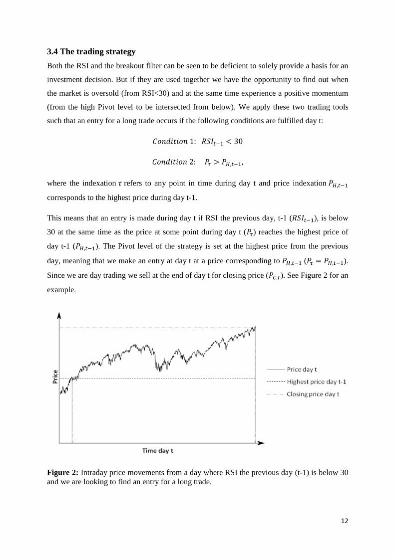
3.4 The trading strategy

Both the RSI and the breakout filter can be seen to be deficient to solely provide a basis for an

investment decision. But if they are used together we have the opportunity to find out when

the market is oversold (from RSI<30) and at the same time experience a positive momentum

(from the high Pivot level to be intersected from below). We apply these two trading tools

such that an entry for a long trade occurs if the following conditions are fulfilled day t:

where the indexation refers to any point in time during day t and price indexation

corresponds to the highest price during day t-1.

This means that an entry is made during day t if RSI the previous day, t-1 ( ), is below

30 at the same time as the price at some point during day t ( ) reaches the highest price of

day t-1 ( ). The Pivot level of the strategy is set at the highest price from the previous

day, meaning that we make an entry at day t at a price corresponding to ( ).

Since we are day trading we sell at the end of day t for closing price ( ). See Figure 2 for an

example.

Figure 2: Intraday price movements from a day where RSI the previous day (t-1) is below 30

and we are looking to find an entry for a long trade.

13

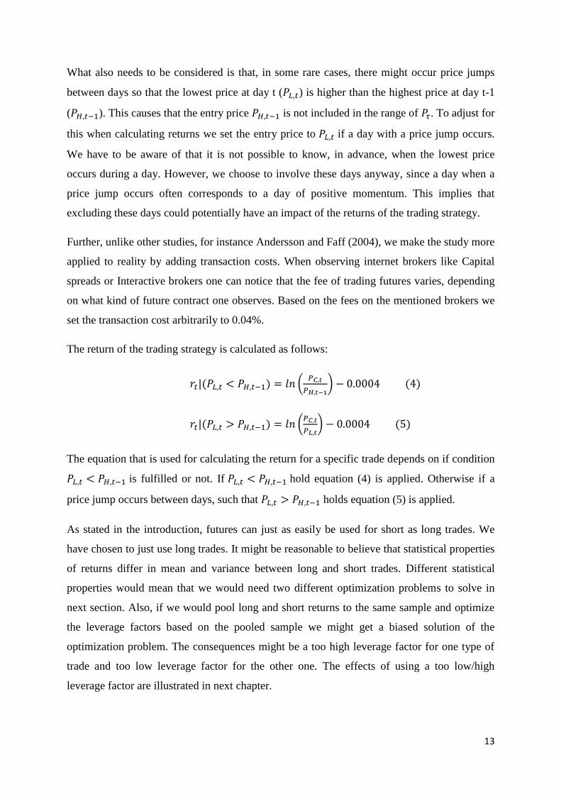
What also needs to be considered is that, in some rare cases, there might occur price jumps

between days so that the lowest price at day t ( ) is higher than the highest price at day t-1

( ). This causes that the entry price is not included in the range of . To adjust for

this when calculating returns we set the entry price to if a day with a price jump occurs.

We have to be aware of that it is not possible to know, in advance, when the lowest price

occurs during a day. However, we choose to involve these days anyway, since a day when a

price jump occurs often corresponds to a day of positive momentum. This implies that

excluding these days could potentially have an impact of the returns of the trading strategy.

Further, unlike other studies, for instance Andersson and Faff (2004), we make the study more

applied to reality by adding transaction costs. When observing internet brokers like Capital

spreads or Interactive brokers one can notice that the fee of trading futures varies, depending

on what kind of future contract one observes. Based on the fees on the mentioned brokers we

set the transaction cost arbitrarily to 0.04%.

The return of the trading strategy is calculated as follows:

The equation that is used for calculating the return for a specific trade depends on if condition

is fulfilled or not. If hold equation (4) is applied. Otherwise if a

price jump occurs between days, such that holds equation (5) is applied.

As stated in the introduction, futures can just as easily be used for short as long trades. We

have chosen to just use long trades. It might be reasonable to believe that statistical properties

of returns differ in mean and variance between long and short trades. Different statistical

properties would mean that we would need two different optimization problems to solve in

next section. Also, if we would pool long and short returns to the same sample and optimize

the leverage factors based on the pooled sample we might get a biased solution of the

optimization problem. The consequences might be a too high leverage factor for one type of

trade and too low leverage factor for the other one. The effects of using a too low/high

leverage factor are illustrated in next chapter.

14

4. Empirical results

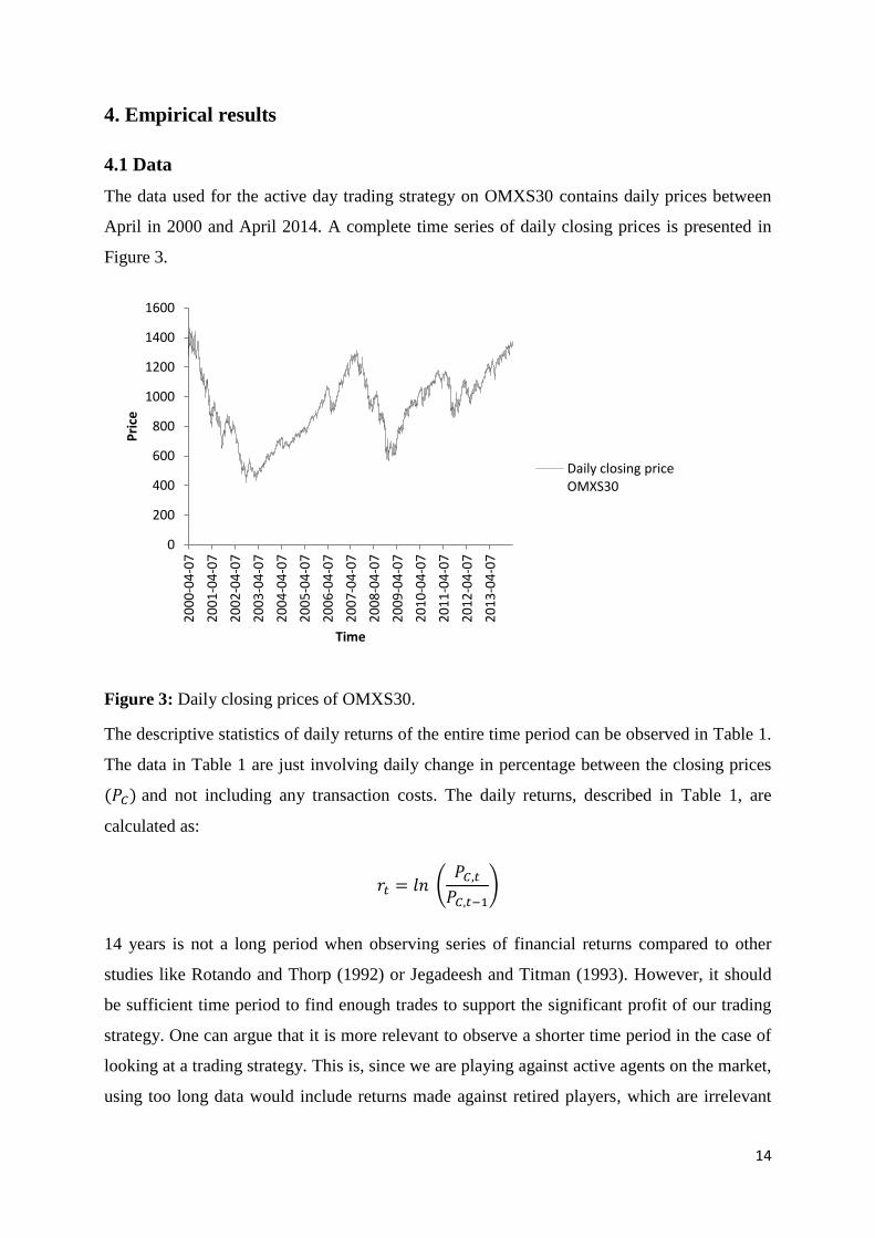
4.1 Data

The data used for the active day trading strategy on OMXS30 contains daily prices between

April in 2000 and April 2014. A complete time series of daily closing prices is presented in

Figure 3.

Figure 3: Daily closing prices of OMXS30.

The descriptive statistics of daily returns of the entire time period can be observed in Table 1.

The data in Table 1 are just involving daily change in percentage between the closing prices

and not including any transaction costs. The daily returns, described in Table 1, are

calculated as:

14 years is not a long period when observing series of financial returns compared to other

studies like Rotando and Thorp (1992) or Jegadeesh and Titman (1993). However, it should

be sufficient time period to find enough trades to support the significant profit of our trading

strategy. One can argue that it is more relevant to observe a shorter time period in the case of

looking at a trading strategy. This is, since we are playing against active agents on the market,

using too long data would include returns made against retired players, which are irrelevant

0

200

400

600

800

1000

1200

1400

1600

20

00

-04

-07

20

01

-04

-07

20

02

-04

-07

20

03

-04

-07

20

04

-04

-07

20

05

-04

-07

20

06

-04

-07

20

07

-04

-07

20

08

-04

-07

20

09

-04

-07

20

10

-04

-07

20

11

-04

-07

20

12

-04

-07

20

13

-04

-07

Pri

ce

Time

Daily closing price OMXS30

15

when looking at a successful trading strategy today. The descriptive statistics of the returns

from the strategy described in section 3.4 is observed in Table 2. For frequency histogram of

the returns from the trading strategy, see appendix C. The returns in Table 2 are calculated as

described in equations (4) and (5).

Table 1: Descriptive statistics of the daily returns of the OMXS30 index between April 2000

and April 2014.

Observations Mean Highest value Lowest value Kurtosis Skewness

3514 -0.001% 9.865 % -8.527 % 6.324 0.073

Table 2: Descriptive statistics of the returns from the trading strategy performed between

April 2000 and April 2014.

Time period Observations Mean Highest value Lowest

value

Kurtosis Skewness

2000-04-07–

2014-04-07

122 0.338% 4.622% -9.414 % 12.418 -1.602

2000-04-07–

2005-08-30

61 0.401% 4.622% -9.414 % 14.423 -2.035

2005-08-31-

2014-04-07

61 0.268% 3.082% -4.084% 4.457 -0.579

As observed in Table 2, 122 trades are obtained from the 14 year long data sample. For the

reasons explained in section 2.2 we also divide the return series of the trading strategy into

two parts. As observed in Table 2 each part contains 61 observations. The amount of 61

observations can possibly cause problems for significance of a positive average return, which

need to be the case for the application of the Kelly criterion. However, Rotando and Thorp

(1992) only use 59 trades and Anderson and Faff (2004) have between 35 and 62 trades on

different future contracts they are trading for a similar purpose as we have in this thesis.

4.2 Profitability test

4.2.1 Model

To establish that the Kelly criterion is applicable we now exercise a profitability test to verify

that the returns’ from the trading strategy described in section 3.4 have a positive mean.

Before estimating the mean we have to consider which estimation method to apply. One

problem by just computing the mean and use a simple t-test is that financial data such as

16

return series generally suffers from heteroscedasticity (Cont, 2001). We also confirm this fact

by using a Breusch-Pagan6 test which shows that we can reject the null hypothesis of

homoscedasticity ( when testing on the entire return series of 122 observations).

Hence, by referring to Cont (2001) and the Breusch-Pagan test we choose to use

heteroscedasticity corrected standard errors (HCSE).

The technique we use to apply the HCSE when estimating the return uses a regression model

as follows:

where the observed returns ( ) is set as the dependent variable. The term is estimating the

mean of the variable , meanwhile corresponds to deviations from that estimated mean.

Due to the heteroscedasticity of the return series the variance of can be described as a

function of as follows (Studenmund, 2011):

where is a variable used to theoretical construct a non constant variance depending on the

size of observation i.

4.2.2 Results

In Table 3 we present the results from the model described by equation 6.

Table 3: Results from the regression models.

Time period Observations (n) Mean return ( ) Robust HCSE P-value

2000-04-07-

2014-04-07

122 0.363% 0.153% 0.028

2000-04-07–

2005-08-30

61 0.401% 0.247% 0.103

2005-08-31-

2014-04-07

61 0.268% 0.183% 0.148

As observed, the mean value of the returns is 0.363% with a P-value of 0.028 when using

HCSE-technique over the entire time period. The interpretation of the P-value in Table 3 is

that we now have quite good evidence that the active trading strategy generates positive

6 Breusch-Pagan is a test of linear heteroscedasticity. Another alternative is White’s general test for

heteroscedasticity. (Greene, 2012)

17

returns over time. The risk of type I error is 2.8%.7 However, we notice some weakness of

significance in the divided samples by observing the P-values to 0.103 and 0.148.

Further, we can also show the dominance of the active day trading strategy over a passive

strategy. In Figure 4 we have allowed for reinvestments of the entire capital in both cases, but

still without any leverage factor. The passive strategy in the Figure 4 is formulated in such a

way that we take a long position with the entire capital in a future contract of OMXS30 and

hold it for 30 days (approximated to 20 trading days). Then repeat the pattern for the next 30

day period etc.. This is done during the same 14 years as the data we use for this paper. The

same transaction cost is used for the passive strategy as for the active strategy. The ingoing

wealth is in both cases set equal to 1.

Figure 4: Comparison of an active and passive strategy on OMXS30.

By observing the last date in Figure 4 a TWR of 1.532 can be observed for the active day

trading strategy. The value of TWR for the passive strategy is observed to a value as low as

0.473. The interpretation from the TWR-values is that the active strategy increases our capital

by 53.2% whilst the buy and hold strategy decreases it by 52.7%. What finally can be

concluded from the significance of the average return and the positive TWR-development of

the active strategy in Figure 4 is that we enough evidence to assume that the Kelly criterion is

applicable on our problem.

7 Type I error refers to the risk of rejecting a true null hypothesis.

0

0,2

0,4

0,6

0,8

1

1,2

1,4

1,6

1,8

20

00

-04

-07

20

01

-04

-07

20

02

-04

-07

20

03

-04

-07

20

04

-04

-07

20

05

-04

-07

20

06

-04

-07

20

07

-04

-07

20

08

-04

-07

20

09

-04

-07

20

10

-04

-07

20

11

-04

-07

20

12

-04

-07

20

13

-04

-07

We

alth

Time

Wealth active daytrading

Wealth buy and hold 30 days

18

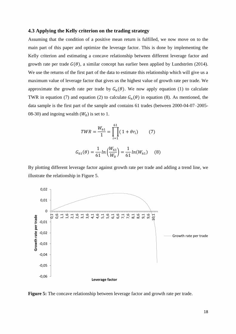
4.3 Applying the Kelly criterion on the trading strategy

Assuming that the condition of a positive mean return is fulfilled, we now move on to the

main part of this paper and optimize the leverage factor. This is done by implementing the

Kelly criterion and estimating a concave relationship between different leverage factor and

growth rate per trade , a similar concept has earlier been applied by Lundström (2014).

We use the returns of the first part of the data to estimate this relationship which will give us a

maximum value of leverage factor that gives us the highest value of growth rate per trade. We

approximate the growth rate per trade by . We now apply equation (1) to calculate

TWR in equation (7) and equation (2) to calculate in equation (8). As mentioned, the

data sample is the first part of the sample and contains 61 trades (between 2000-04-07–2005-

08-30) and ingoing wealth ( ) is set to 1.

By plotting different leverage factor against growth rate per trade and adding a trend line, we

illustrate the relationship in Figure 5.

Figure 5: The concave relationship between leverage factor and growth rate per trade.

-0,06

-0,05

-0,04

-0,03

-0,02

-0,01

0

0,01

0,02

0,1

0,6

1,1

1,6

2,1

2,6

3,1

3,6

4,1

4,6

5,1

5,6

6,1

6,6

7,1

7,6

8,1

8,6

9,1

9,6

10

,1

Gro

wth

rat

e p

er

trad

e

Leverage factor

Growth rate per trade

19

By observing figure 5 we note that we have a clear strictly concave relationship between

leverage factor and growth rate per trade. The relationship reminds us of the same relationship

from the bet fraction from the example from the lottery in chapter 2 which was also described

in Figure 1. This does also support what can be expected from the theory of Kelly criterion.

The maximum value of growth rate per trade of 1.649% is achieved when the leverage factor

is set to 6.7.

4.4 Comparing the optimized θ to θ=1

We are now interested in whether the Kelly criterion maximizes the profits of our trading

strategy. We already know that without leverage factor ( ) significant profit can be

achieved. As recalled from the introduction is the same as not regarding investment

size and not involving money management. That is why is used as comparison with the

optimized . We now test the application of the Kelly criterion by setting and

compare the development of TWR for the two different leverage factors used on the second

part of the sample of returns (between 2005-08-31-2014-04-07).

Figure 6: Comparison of TWR-development of the optimized leverage factor vs. no leverage

factor.

As observed in Figure 6, we notice an improvement of wealth development when . The

optimized leverage factor results in a TWR of 2.249, meanwhile the result of trading with

leverage factor just gives a TWR of 1.170.

0

0,5

1

1,5

2

2,5

TWR

Time

θ=1

θ=θ*

20

The corresponding values of growth rate per trade from the =1 and =6.7 for the second part

of the time period can easily be calculated by using equation 8:

As we notice the optimal value of results in a growth rate per trade of 1.329% which is not

very far from the maximum value of 1.649% from the concave curve in Figure 5. Further, all

results of the total returns achieved from trading during the second part of the time series are

presented in Table 5 in section 4.7.

4.5 Using a high leverage factor

Even if we adopt this problem as a risk neutral investor the risks of increasing the leverage

factor need to be considered. By observing the optimized in Figure 6 one can notice big

fluctuations both up- and downward which indicates that we cannot reject the risky aspect of a

high leverage factor. As recalled from Kelly (1956) and the lottery example in section 2.2 one

should always find the balanced leverage factor, since in case of a “bad” trade a too high

leverage factor limit the reinvestment possibilities significantly.8

To clarify and illustrate the risks of a high leverage factor we choose to set the leverage factor

arbitrarily high to and observe the effects of the TWR development with a value of

set to 1.

8 The balanced leverage factor is the same in active futures trading as the optimal bet fraction is in the lottery

example in section 2.2.

21

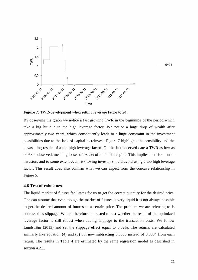
Figure 7: TWR-development when setting leverage factor to 24.

By observing the graph we notice a fast growing TWR in the beginning of the period which

take a big hit due to the high leverage factor. We notice a huge drop of wealth after

approximately two years, which consequently leads to a huge constraint in the investment

possibilities due to the lack of capital to reinvest. Figure 7 highlights the sensibility and the

devastating results of a too high leverage factor. On the last observed date a TWR as low as

0.068 is observed, meaning losses of 93.2% of the initial capital. This implies that risk neutral

investors and to some extent even risk loving investor should avoid using a too high leverage

factor. This result does also confirm what we can expect from the concave relationship in

Figure 5.

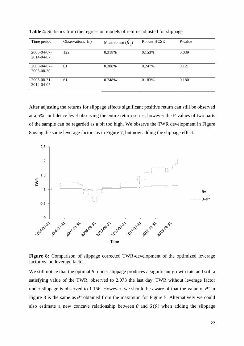
4.6 Test of robustness

The liquid market of futures facilitates for us to get the correct quantity for the desired price.

One can assume that even though the market of futures is very liquid it is not always possible

to get the desired amount of futures to a certain price. The problem we are referring to is

addressed as slippage. We are therefore interested to test whether the result of the optimized

leverage factor is still robust when adding slippage to the transaction costs. We follow

Lundström (2013) and set the slippage effect equal to 0.02%. The returns are calculated

similarly like equation (4) and (5) but now subtracting 0.0006 instead of 0.0004 from each

return. The results in Table 4 are estimated by the same regression model as described in

section 4.2.1.

0

0,5

1

1,5

2

2,5

TWR

Time

θ=24

22

Table 4: Statistics from the regression models of returns adjusted for slippage

Time period Observations (n) Mean return ( ) Robust HCSE P-value

2000-04-07-

2014-04-07

122 0.318% 0.153% 0.039

2000-04-07–

2005-08-30

61 0.388% 0.247% 0.121

2005-08-31-

2014-04-07

61 0.248% 0.183% 0.180

After adjusting the returns for slippage effects significant positive return can still be observed

at a 5% confidence level observing the entire return series; however the P-values of two parts

of the sample can be regarded as a bit too high. We observe the TWR development in Figure

8 using the same leverage factors as in Figure 7, but now adding the slippage effect.

Figure 8: Comparison of slippage corrected TWR-development of the optimized leverage

factor vs. no leverage factor.

We still notice that the optimal under slippage produces a significant growth rate and still a

satisfying value of the TWR, observed to 2.073 the last day. TWR without leverage factor

under slippage is observed to 1.156. However, we should be aware of that the value of in

Figure 8 is the same as obtained from the maximum for Figure 5. Alternatively we could

also estimate a new concave relationship between and when adding the slippage

0

0,5

1

1,5

2

2,5

TWR

Time

θ=1

θ=θ*

23

effect. This would likely marginally change the , and thereby might result in a slightly

higher TWR for the slippage effect than the one we obtain in figure 8.

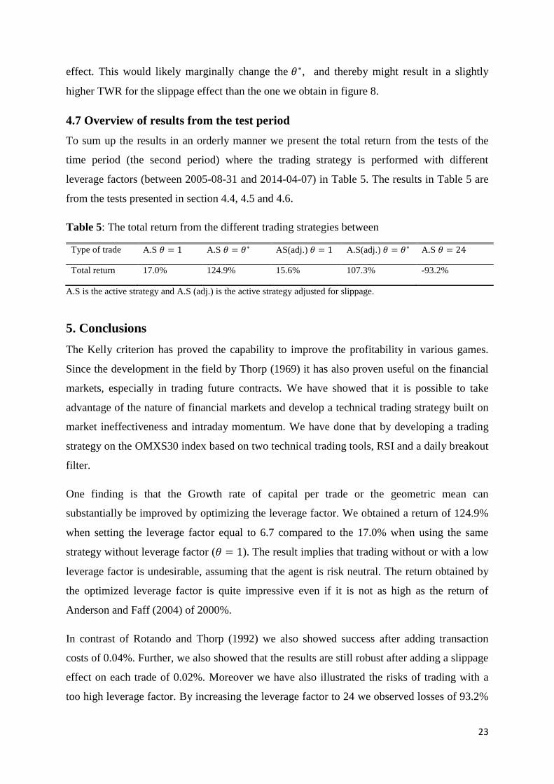
4.7 Overview of results from the test period

To sum up the results in an orderly manner we present the total return from the tests of the

time period (the second period) where the trading strategy is performed with different

leverage factors (between 2005-08-31 and 2014-04-07) in Table 5. The results in Table 5 are

from the tests presented in section 4.4, 4.5 and 4.6.

Table 5: The total return from the different trading strategies between

Type of trade A.S A.S AS(adj.) A.S(adj.) A.S

Total return 17.0% 124.9% 15.6% 107.3% -93.2%

A.S is the active strategy and A.S (adj.) is the active strategy adjusted for slippage.

5. Conclusions

The Kelly criterion has proved the capability to improve the profitability in various games.

Since the development in the field by Thorp (1969) it has also proven useful on the financial

markets, especially in trading future contracts. We have showed that it is possible to take

advantage of the nature of financial markets and develop a technical trading strategy built on

market ineffectiveness and intraday momentum. We have done that by developing a trading

strategy on the OMXS30 index based on two technical trading tools, RSI and a daily breakout

filter.

One finding is that the Growth rate of capital per trade or the geometric mean can

substantially be improved by optimizing the leverage factor. We obtained a return of 124.9%

when setting the leverage factor equal to 6.7 compared to the 17.0% when using the same

strategy without leverage factor ( ). The result implies that trading without or with a low

leverage factor is undesirable, assuming that the agent is risk neutral. The return obtained by

the optimized leverage factor is quite impressive even if it is not as high as the return of

Anderson and Faff (2004) of 2000%.

In contrast of Rotando and Thorp (1992) we also showed success after adding transaction

costs of 0.04%. Further, we also showed that the results are still robust after adding a slippage

effect on each trade of 0.02%. Moreover we have also illustrated the risks of trading with a

too high leverage factor. By increasing the leverage factor to 24 we observed losses of 93.2%

24

of the initial capital showing that even risk neutral and to some extent risk loving investors

need to consider the leverage factor instead of just use the highest possible leverage factor

which also maximizes the expected value of a single trade. One shortcoming of this study is

the lack of sample size; one can argue that a greater data set would give better precision in

determining what leverage factor to use. We can also observe the shortcoming of the few

observations by observing the P-values from the profitability tests.

Instead of just finding a strategy that tells us when to buy and sell, we have like earlier studies

(e.g., Tharp 1997) confirmed the relevance of money management. We have, in some extent,

contributed with further evidence of the Kelly criterion’s functionality on the financial

markets. If we were interested in developing the study further we could try a different strategy

or apply it on a different underlying asset.

Further we could, like Lundström (2014), add stop losses to the study. In that way many of

the largest negative returns would get reduced. We could also expand the study for short

trades, and show that the different statistical properties of those returns would lead to another

optimal leverage factor. The field of money management and different applications of the

Kelly criterion are indeed interesting for further research and should be of great interest for

successful traders and various portfolio managers.

25

References

Anderson, J. A. and Faff, R. W. (2004): “Maximizing futures returns using fixed fraction

asset allocation.” Applied Financial Economics, 14, 1067–1073.

Balsara, N. J. (1992): Money Management Strategies for Futures Traders, New York: Wiley.

Barberis, N., A. Shleifer, and R. Vishny (1998): “A Model of Investor Sentiment,”

Journal of Financial Economics, 49, 307–343.

Capital spreads, transaction costs of futures trading, 15th

May 2014

<http://www.capitalspreads.com/spread-betting/market-information >

Cont, R. (2001): “Empirical properties of asset returns: stylized facts and statistical issues.“

Quantitative Finance, 1, 223-236.

Crabel, T. (1990): Day Trading With Short Term Price Patterns Day Trading With Short

Term Price Patterns and Opening Range Breakout, Greenville, S.C. : Traders Press

Daniel, K., D. Hirshleifer, and A. Subrahmanyam (1998): “Investor Psychology and

Security Market Under- and Overreactions,,” Journal of Finance, 53, 1839–1885

Fama, E. (1965): “The Behavior of Stock Market Prices,” Journal of Business, 38, 34–105.

Gehm, F. (1983): Commodity Market Money Management, New York: Wiley

Greene, W.H. (2012). Econometric analysis, (7. Ed.), Boston: Pearson, 315-317

Holmberg, U., C. Lönnbark, and C. Lundström (2013): ”Assessing profitability of Intraday

Opening Range Breakout Strategies,” Finance research letters, 10, 27-33.

Interactive brokers, transaction costs of futures trading, 15th

May 2014

<https://www.interactivebrokers.com/en/index.php?f=commission&p=futures>

Jegadeesh, N. and S. Titman (1993): “Returns to Buying Winners and Selling Losers:

Implications for Stock Market Efficiency,” Journal of Finance, 48, 65–91.

26

Kelly, Jr, J. L. (1956): “A new interpretation of information rate,” The Bell System Technical

Journal, 35, 917–926.

Lim, K and R. Brooks (2011): “The evolution of stock market efficiency over time: a survey

of the empirical literature,” Journal of Economic Surveys, 25, 69-108.

Lundström, C. (2013): ”Day Trading Profitability across Volatility States: Evidence of

Intraday Momentum and Mean-Reversion” Umeå Economic Studies, 861. Umeå University.

Lundström, C. (2014): “Money management with optimal stopping of losses for maximizing

the returns of futures trading“. Umeå Economic Studies, 884. Umeå university.

Malkiel, B. G. (1996): A Random Walk Down Wall Street, W. W. Norton

Pring, M. J. (1991) Technical analysis explained. New York: McGraw-Hill.

Rotando, L. M. and E.O. Thorp (1992): “The Kelly criterion and the stock market,” The

American Mathematical Monthly, 99, 922–931.

Sewell, M. (2011): “Money Management.” Research note RN/11/05. The Department of

Computer Science. London University.

Shiller, R. (2001): “Human behavior and the efficiency of the financial system” Cowles

foundation for research in economics, 1306-1334. Yale university.

Studenmund, A. H. (2011). Using econometrics: a practical guide. (6. ed.), Boston: Pearson,

351-352

Sullivan, R., A. Timmermann, and H. White (1999): “Data-Snooping, Technical Trading Rule

Performance, and the Bootstrap.” The Journal of Finance, 54, 1647-1691.

Tharp, Van K. (1997): “Special Report on Money Management” I.I.T.M., Inc. USA

Thorp, E.O. (1969): “Optimal gambling systems for favorable games” Review of the

International Statistical Institute, 37, 273–293.

27

Vince, R. (1990): Portfolio Management Formulas: Mathematical Trading Methods for the

Futures, Options and Stock Markets, New York: Wiley

Wang, C., and M. Yu (2004): “Trading Activity and Price Reversals in Futures Markets.”

Journal of Banking and Finance, 28, 1337-1361.

Wilder, J. W., Jr. (1978). New concepts in technical trading systems. Greensboro, NC: Hunter

Publishing Company.

28

Appendix

A. How to practically obtain θ

To show how we can manipulate the leverage factor to be equal to we assume a future

contract of an asset (A) with price PA. Further we assume that the future contract has a fixed

specific leverage factor ( ), where . If we at time t spend the entire capital ( ) on

futures of asset A the capital at time t+1 ( ) is given by:

,where can be calculated as:

If we were able have a future contract with the leverage factor we could describe the capital

at time t+1 as:

However, since the future contract of an asset generally has a fixed leverage factor (L) we

need an alternative way to obtain the leverage factor . To obtain the leverage factor we

buy future contracts of asset A by an amount corresponding to a fraction

of our capital. It

follows that:

Since

is the amount we invest at time t the rest of the capital is:

By investing

at time t we can now describe the capital at time t+1 as:

29

Since we now know the amount we should invest we buy the amount of future contract

corresponds to the fraction of our capital that gives us the desired leverage factor. An

important note is that even if the price of a certain future contract could be high the platforms

for trading generally allow the agent to buy fractions of future contracts.

B. Relative strength index

Note that “Average price fall last 14 days” could be equal to zero if the price increases

for 14 days in a row. Since RS is not defined for we instead use limits and

show:

It follows that:

30

C. Frequency histogram of returns

Figure 9: Frequency histogram of returns.

0

5

10

15

20

25

30

35

40

45

50

-0,1

-0,0

9

-0,0

8

-0,0

7

-0,0

6

-0,0

5

-0,0

4

-0,0

3

-0,0

2

-0,0

1

0

0,0

1

0,0

2

0,0

3

0,0

4

0,0

5

0,0

6

0,0

7

0,0

8

0,0

9

0,1

Mo

re

Frequency