monitoring and modelling of coastal currents and

29Geo-Eco-Marina 20/2014

1. INTRODUCTION

A coastal ecosystem represents a rich and fragile re-source, subject to modifications due to natural variations and human activities (Roberts, 1980; Wood et al., 1993). Conse-quently, the planning and the management of coastal activi-ties is of fundamental importance, even more when a waste-water sea outfall system has its ultimate sink in the coastal water. Despite the natural processes of marine dilution and self-depuration, both environmental quality standards of the receptor and physicochemical parameters of the discharge itself should be continuously monitored to guarantee the re-spect of the prescribed limits and the safeguard of the coastal ecosystem. Therefore, it seems unavoidable the monitoring

of the plant outfall in terms of (i) physicochemical and bac-teriological measurements, and (ii) current, wave and wind measurements (Nash and Jirka, 1996; Mossa, 2004; Chin, 1988; Chyan and Hwung, 1993; Davies et al., 1997; Hwung et al., 1994). Only in this way, the ecosystem could be pro-tected against risks, and the specific uses of the zone could also be preserved (i.e. tourism, swimming, mussel farms). The main aim of an outfall pipe is to issue the wastewater where the natural assimilative capacity of the sea could guarantee the minimal environmental impact, i.e. at a distance where the hydrodynamic effects can assure the fulfilment of qual-ity standards set by regulation and preserve the shoreline. Therefore, it is crucial to provide investigations which can de-

MONITORING AND MODELLING OF COASTAL CURRENTS AND WASTEWATER DISCHARGE:

A CASE STUDYFrancesca De serIO(1), MOulDI Ben MeFTaH(2), MIcHele MOssa(3)

(1) DICATECh, Technical University of Bari, Via E. Orabona 4, 70125 Bari, Italy, e-mail: [email protected]; corresponding author

(2) DICATECh, Technical University of Bari, Via E. Orabona 4, 70125 Bari, Italy, e-mail: mouldi.benmeftah@ poliba.it

(3) DICATECh, Technical University of Bari, Via E. Orabona 4, 70125 Bari, Italy, e-mail: [email protected]

Abstract. The coastal areas neighbouring wastewater outfalls are particularly sensitive and vulnerable, therefore they should be continuously monitored. The present paper examines the results of a monitoring survey carried out in July 2001 offshore the Bari town, in the Southern Adriatic Sea (South Italy), close to the outfall of its wastewater treatment plant, named Bari East. Measurements of horizontal and vertical velocity components were carried out with a Vessel Mounted Acoustic Doppler Profiler. Also salinity and temperature were assessed at the same time and locations by means of a CTD probe. The investigation confirms the pivotal role played by currents magnitude and direction, wind, tide and stratification in the process of diffusion and dispersion of passive tracers (such as temperature and salinity). As a second step, the MIKE 3FM, a 3D numerical model by the Danish Hydraulic Institute (DHI) is tested to reproduce the hydrodynamic current pattern and the diffusion of the plume in the target area. The model was implemented with initial and boundary conditions relative to the survey day and the assessed measurements were used to calibrate it, by tuning some parameters, such as the wind drag coef-ficient, the bottom roughness and a turbulence closure model coefficient. A satisfactory agreement was found between field measurements and model results, showing that in the target area the modelled hydrodynamics was prevalently influenced by the wind drag coefficient and less affected by bottom roughness and turbulence. The present approach confirms that, once calibrated and validated, a numerical model could be a powerful instrument to sup-port both planning and management of coastal activities. In fact, it could allow to predict the possible dispersion of a polluting tracer when a scenario is established, thus providing some useful maps of spreading.

Keywords: wastewater outfall, coastal currents, monitoring, numerical modelling.

30 Geo-Eco-Marina 20/2014

Francesca De Serio, Mouldi Ben Meftah, Michele Mossa – Monitoring and modelling of coastal currents and wastewater discharge

termine the local effects and to be familiar with the sea cur-rent circulation in the outfall region. These analyses should be carried out at a preliminary stage, when planning the outfall, and also successively, during the functioning of the outfall, to monitor its environmental impact (Mossa, 2006). The meas-urements necessary for monitoring cannot be concentrated in the wastewater outfall pipe zone only, but should be ex-tended to a neighbouring area, with the extension depend-ing on the wastewater discharge, its polluting charge and the magnitude of the sea currents and winds typical in the zone of interest. In fact, the so called near field region, responsi-ble for rise height, initial mixing and dilution, occupies a very small fraction of the overall impact of the discharge (Roberts, 1980). Beyond the near field, the waste field drifts with the sea current and is diffused by turbulence in a region called the far field, where the rate of mixing is much slower.

In any case, collecting a large amount of reliable and continuous measurements of coastal outfall plumes is chal-lenging (Mossa, 2006; De Serio and Mossa, 2014), because of technical and economic limitation (i.e. high costs, variability of discharge flowrate, currents, stratification and the wide-spread area to be monitored). Numerical models could be a useful task in this sense for both coastal and offshore design and management, allowing to describe and even forecast the current flow pattern, responsible of numerous marine phe-nomena such as mixing and dispersion of pollutants, but also sediment transport and current-induced structural loading. All these phenomena, in fact, even if governed by different temporal and spatial scales, are in any way strictly dependent on the current magnitudes and directions. A numerical mod-el could represent a more rapid and a less expensive solution, taking into account that it can simulate the hydrodynamics of extended areas with the desired level of accuracy and in relatively short times. Nevertheless, to be accurate, it needs for reliable initial and boundary conditions and it should be calibrated and validated by means of measured data (Bruno et al., 2009; De Serio et al., 2007; Scroccaro et al., 2010). There-fore, both field measurements and numerical modelling should be coupled to guarantee a useful support to local au-thorities in coastal management and safeguard.

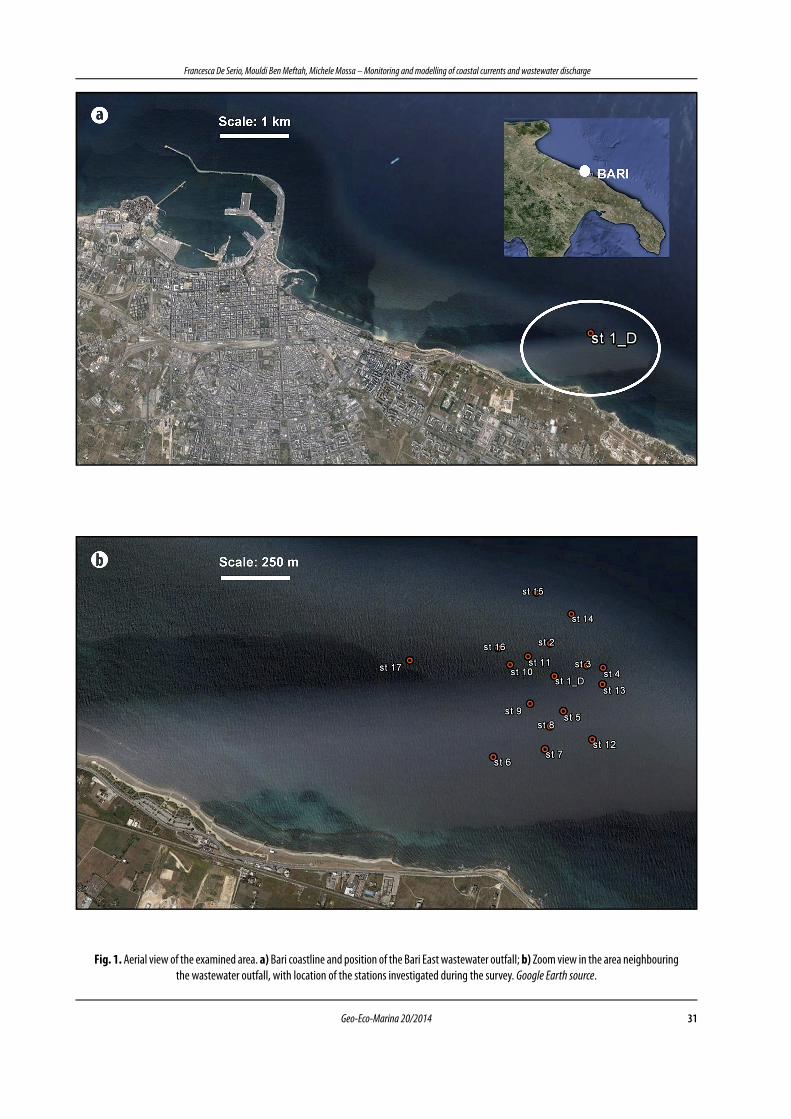
The first aim of the present study is to analyse the field data taken during a monitoring survey day in the Southern Adriatic Sea (Fig. 1a). The measurements were carried out by the research group of the Department of Civil, Environmental, Building Engineering and Chemistry of the Technical Univer-sity of Bari, on 25 July 2001, offshore Bari town. The investigat-ed area neighboured the outfall of the Bari East wastewater treatment plant and 17 stationing points were investigated (Fig. 1b), with local depths in the range of 10m÷20m. The three velocity components were measured by means of a Vessel Mounted Acoustic Doppler Current Profiler (VM-AD-CP). At the same time and locations also a CTD recorder was used to measure water temperature and salinity, in order to get information about the presence of a buoyancy jet and of

a possible stratification. In this way, both vertical profiles and horizontal maps of the assessed data were deduced.

As a second step, the paper evaluates the ability of the numerical model MIKE 3FM by DHI (Moharir et al., 2014) to reliably reproduce the hydrodynamic circulation and the plume diffusion in the survey period. The computational do-main was discretized by a mesh, with a finer resolution ap-proaching the coastline. The model was calibrated by tuning some relevant parameters such as the wind drag coefficient, the bottom roughness and a turbulence closure model coef-ficient. Five different tests were run and a relative error be-tween measured and computed velocity values was analysed to derive the best matching condition.

The paper is structured as follows. Section 2 describes the survey equipment and analyses the assessed data. In Section 3, the used numerical model is described as well as the five calibration tests. In Section 4, the comparison among measurements and results is shown, pointing out the princi-pal findings.

2. EXPERIMENTAL SET UP AND ACQUISITION

2.1 Used equipment and survey description

As mentioned above, a monitoring cruise was carried out on 25.07.2001 by the research group of the Department of Civil, Environmental, Building Engineering and Chemistry of the Technical University of Bari. A Nortek AWAC (Acoustic Wave And Current) VM-ADCP was used to measure the sea three-current-velocity components. It was connected to a gyro and a DGPS in order to take into account the vessel ve-locity and thus to acquire the current velocity with respect to the seabed. Moreover, the DGPS was used to locate the pre-determined stationing points. The main features of the AWAC current meter system are shown in Table 1. Its stand-ard configuration has three beams 120º apart, slanted at 25°, and one vertical, whose opening angle is 1.7°. During all the surveys, the measurements of the flow were assessed with an acquisition frequency of 0.5Hz, therefore only the veloci-ties averaged over a time interval of about 10 minutes are examined in the present paper. This acquisition time interval guaranteed that the measurements were stationary, as con-firmed by the time moving average of the measured velocity components and of their variances. The measurements were acquired starting from 4m below the water surface, as it was the blanking distance of the instrument. The bin size was fixed and equal to 1.5m, with bins number depending on the investigated local depths. The measurements of all the sur-veys were assessed by anchoring the boat and acquiring the velocities for a total time not less than 5 minutes for each in-vestigated station, in order to reach a stationary measure. The mounting of the probe required the use of stainless steel tu-bular elements supported by an anchorage stirrup attached to the boat, with a total length of 3.5 m.



Fig. 1. Aerial view of the examined area. a) Bari coastline and position of the Bari East wastewater outfall; b) Zoom view in the area neighbouring the wastewater outfall, with location of the stations investigated during the survey. Google Earth source.



A CTD recorder system by Idronaut Srl was used to meas-ure the water temperature and salinity along the water col-umn, during the same time interval and at the same location. Table 1 shows the accuracy and resolution of the main quan-tities of the CTD recorder system. Wind data were derived from the ISPRA database (Italian Institution for Environmen-tal Protection and Research) and were also verified by the lo-cal acquisition by means of an anemometer.

2.2 Field data analysis

During the survey, seventeen vertical profiles were ana-lysed, starting from 8:10 and finishing at 11:50, in an area covering approximately 800m x 700m. In Figure 1b, the in-vestigated stations are displayed, while their geographical coordinates, depths and measuring time are summed up in Table 2. On average, during the measurement time, the

recorded wind was coming from ENE and had an intensity equal to 5 m/s.

The wastewater outfall system of Bari East is composed of a 900m long submarine pipe from the shoreline, whose direction is almost normal to the shoreline. In the shallow water this steel conduit with a diameter of 1.2m is covered, in order to be protected from the wave motion field. The end part of the pipe constitutes the diffuser, in polythene, which lies directly on the sea bottom. As shown in Figure 1b, sta-tion 1_D was the nearest to the diffuser, where the rising of a jet was visible due to the bulging surface and to the more soft water colour. Stations 2, 3 and 4 were located offshore the outfall diffuser as well as stations 14 and 15, which were the most distant from the coast, along the 20m bathymetric line. Stations 10, 11 and 16 were located approximately at the

Table 1. Main characteristics of the VM-ADCP system and of the CTD probe.

Probe Type Value

VM-ADCP

Acoustic frequency 600 KHz

Velocity range ± 10 m/s horizontal; ± 5 m/s vertical

Velocity accuracy 1% of measured value ± 0.5 cm/s

CTD

Pressure range 0÷7000 m

Pressure accuracy 1‰

Temperature range -5÷35 °C

Temperature accuracy 5‰

Table 2. Geographical coordinates. Gauss-Boaga reference system used.

Stations Longitude [m] Latitude [m] Time [hour:min] Local heights [m]

St 1_D 2682191.72 4553764.29 08:17 18.0

St 2 2682175.73 4553921.00 08:49 19.0

St 3 2682332.79 4553823.40 08:58 17.5

St 4 2682402.5 4553816.17 09:08 17.0

St 5 2682226.32 4553605.66 09:16 16.0

St 6 2681933.2 4553387.34 09:26 12.5

St 7 2682145.66 4553432.37 09:41 14.5

St 8 2682168.08 4553535.06 09:54 16.0

St 9 2682085.54 4553631.86 10:06 16.0

St 10 2682000.65 4553808.59 10:15 17.4

St 11 2682078.63 4553852.53 10:25 18.2

St 12 2682342.72 4553485.51 10:46 14.7

St 13 2682396.85 4553737.63 10:57 16.0

St 14 2682273.59 4554072.23 11:08 20.0

St 15 2682119.75 4554172.67 11:20 20.0

St 16 2681948.62 4553886.08 11:33 17.6

St 17 2681565.67 4553806.52 11:41 14.5



same depth of the diffuser, i.e. along the 18m bathymetric line. Stations 5, 6, 7, 8, 9, 12 and 17 were onshore the diffuser at a depth of 15m on average. In order to show the principal pattern of the current, Figure 2 plots a map of the measured horizontal velocity for heights in the range z = -4m ÷ -11.5m, z being the vertical height with zero at the sea surface. For the most part of the stations the flow seems wind driven, in fact it is directed towards NNW near the surface, quite parallel to the coast, except for stations 2, where it curves towards W and for stations 3, 12 and 8 where it reverses towards SE. With deepening heights, a prevailing clockwise rotation of the flow can be noted, along the vertical. The horizontal ve-locity components reach values of about 0.2 m/s. As an ex-ample, Figure 3a and Figure 3b show the horizontal velocity vectors at heights z = -4m and z = -10m, respectively. The red vectors are the measured velocities while black vectors are those deduced from a linear interpolation, in order to bet-ter represent the current trend in the target area. Figure 3a shows a more intense current directed towards NNW, in the northern part of the area, while a reversal of the current to-wards SSE is visible in the southern part, characterized by less

intensity. At 10m from the surface (Fig. 3b) the current in the north-western part of the area rotates towards N, while the reversing southern flow becomes more intense. Velocity di-rections remain quite invariant with increasing height, while velocity values reduce. Also the vertical velocity components are plotted in the same Figure by means of the contour lines, with positive values for upward vertical velocity and negative values for downward vertical velocity. The analysis of Figure 3a and Figure 3b highlights that, even if the vertical velocity components are about an order of magnitude less than the horizontal ones, a vertical circulation is present in any case. A vertical flow was directed upward at deeper heights, so that the measurements detected the outflow.

The vertical profiles of measured temperature T and salini-ty S are plotted in Figure 4 and Figure 5, respectively. It is worth noting that, in all the investigated stations, an increase in tem-perature of about 1C° from the sea bottom up to z/h=0.45 is ob-served. For z/h>0.45 the temperature remains quite constant, with slight variations near the surface, except for Station 1_D where it sharply decreases in the upper layer (0.75<z/h<1). The vertical salinity profiles have a flat trend from the bottom up to

Fig. 2. Map of measured horizontal velocities in the investigated stations at some selected heights. Gauss-Boaga reference system used.



Fig. 3. Horizontal map of the measured velocity at a) height z=-4m and b) height z=-10m from the sea surface (red arrows are the measured currents, black arrows are the interpolated ones). Gauss-Boaga reference system used.



z/h~0.75, characterized by an average value of 37.9psu, while

in the range 0.75<z/h<1 the salinity decreases of about 40%

in all the stations. In station 1_D, the salinity reduction is more

marked, reaching values of 36.2 psu at the surface. This vertical

behavior, shown in both Figure 4 and Figure 5, illustrates the

presence of a stratification in the upper layer of the water col-

umn, particularly for stations st 1_D, st 10, st 11, st 16 and st 17

which is consistent with the presence and the diffusion of the

plume due to the current moving towards NNW. The presence

of the buoyancy jet from the diffuser, which spreads and en-

larges towards the surface, is further observed in the salinity

map plotted at the height of z=-0.6m (Fig. 6).

Fig. 4. Vertical profiles of the measured temperature T [C°] in the investigated stations.

Fig. 5. Vertical profiles of the measured salinity S [psu] in the investigated stations.



Smaller values of salinity are present close to the location of the wastewater outfall and a gradual increase of salinity to-wards the NW is evident. This elongated shape of the salinity map confirms a diffusion process towards the NW, consistent with the velocity measurements, so that the plume is mixed and transported by the observed current.

3. MODEL DESCRIPTION AND NUMERICAL RUNS

3.1. Numerical model

The numerical model MIKE 3D with Flexible Mesh (Mo-harir et al., 2014) developed by DHI (Danish Hydraulic Insti-tute) was used in the present study. It is based on the solu-tion of the incompressible Reynolds averaged Navier-Stokes equations, thus solving the conservation equation of conti-nuity, momentum, temperature, salinity and turbulent ki-netic energy. The vertical discretization was operated by six sigma layers, while in the horizontal plane a triangular mesh was used for the computation, with a finer resolution ap-proaching the shoreline and the wastewater outfall. The used bathymetry and the shoreline were derived from the data by

the Hydrographic Institute of the Italian Navy and were in-terpolated on a mesh with 2592 nodes. The simulated area extended parallel to the coast for about 20km and offshore for about 7km, where the open boundary was located.

The integration method used during the calculation was the Runge-Kutta algorithm of the second order. In the pre-sent study, the turbulence at the subgrid scale in the horizon-tal plane was modelled by the classical Smagorinsky model (Blumberg and Mellor, 1987). In this case, the horizontal mix-ing coefficient AM for momentum, i.e. viscosity (as well as for tracers, i.e. diffusivity) were calculated by the Smagorinsky formulation, such that:

A C x y

ux

vx

uy

vyM s=

∂∂

+

∂∂

+∂∂

+

∂∂

∆ ∆

2 2 2

(1)

where u and v are the velocity components along the x (east-ward) and y (northward) directions, Δx and Δy are the spac-ings along these directions and Cs is the Smagorinsky coef-ficient, tuned for our calibration purposes. The vertical eddy viscosity was provided by the log law formulation.

Fig. 6. Horizontal map of the measured salinity S [psu] in the investigated area, at a distance of z = -0.6m from the surface. Gauss-Boaga refer-ence system used.



The bottom stress τb was expressed by the quadratic fric-tion law

τ ρb b b bC u u=

(2)

where Cb is the drag coefficient, ρ is the water density and ub is the bottom velocity. The drag coefficient depends on the bottom roughness z0, according to

C

kzz

b

b

=

1

1

0

2

log

(3)

assuming a velocity logarithmic profile between the seabed and the height zb where ub is detected, with the von Karman constant k=0.4.

The wind stress τw was evaluated in a similar way:

τ ρw a w w wC u u=

(4)

where ρa is the air density, τw is the wind speed and Cw is the wind drag coefficient.

3.2 Simulations settings

The calibration procedure was carried out in the follow-ing way. Previous researches (De Serio et al., 2007) highlight-ed that the model is strongly sensitive to the variability in the bottom roughness z0 and in the wind drag coefficient Cw. Moreover, the horizontal mixing coefficient of the turbulence model seemed to affect specifically the currents patterns. For these reasons, the parameters z0, Cw and Cs were chosen as reference parameters to calibrate the model. They were tuned till reaching the best matching between field veloci-ties and model outputs.

Referring to the input forcings, the simulations were run in baroclinic mode. The assigned temperature and salinity along the water column were derived from Figure 4 and Fig-ure 5, thus taking into account the slight observed superficial stratification. At greater heights, the values of T=24°C and S=37.8psu were imposed, while values of T and S equal to 24.3°C and 37.6psu, respectively, were imposed for z/h>0.8. The wind was imposed as a time-varying forcing action. It was reliably considered homogeneous in space, being rather limited the domain of interest. The tidal contribution was im-posed along the open boundaries of the domain as a time-

varying total sea level. Both wind and sea level data of the investigated period were derived as time series from the IS-PRA database (www.idromare.it). The wastewater outfall was simulated by means of a continuous source with a constant flow rate of 1.05m3/s, an average temperature of 20°C and an average salinity of 1.5psu, according to the information about the discharge derived from the Acquedotto Pugliese spa, i.e. the company managing the treatment plant.

Five different runs were executed. Each test had a total duration of 25 days, starting from 01.07.2001 at 00:00 and ending at 00:00 of 26.07.2001. In this way, the possible tran-sient effects were limited to the first part of the simulations, while a stationary condition was reached in the survey day.

The values assumed by the calibration parameters in each test are shown in Table 3. The bottom roughness was switched between z0=0.05m and z0=0.10m, following some subaqueous investigations which proved the presence of de-bris and ripples offshore the Bari coast. The wind drag coef-ficient was switched between 0.0025 according to classical literature values (Wu, 1980) and 0.005, a higher value tested in previous experimental works (De Serio et al., 2007). It was highlighted that for a limited domain (far from the oceanic conditions) the wind drag coefficient should be increased to correctly reproduce the wind effect. The Smagorinsky coef-ficient was switched between the default value 0.28 and the value 0.6.

4. ANALYSIS AND DISCUSSION OF THE COMPUTED RESULTS

4.1. Velocity patterns

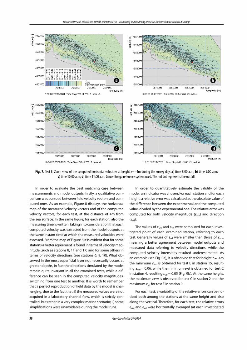
As an example, in Figure 7, for test E the horizontal com-puted current patterns in the time interval of the survey are shown at the height z=-4 m, with hourly frequency (starting from 8:00) during the survey day. The variability of the cur-rent direction and magnitude is evident. Figure 7 plots at hour 8:00 an inversion of the current, which leaves the coast-line and bends towards NW. A more intense northwesterly flow is evident at greater heights. This system feeds a small clockwise gyre approaching the Port of Bari. In the follow-ing hours the gyre becomes less intense, its branches being overwhelmed by the flow coming from SE, whose intensity increases with time (as shown at hour 11:00).

Table 3. Calibration coefficients used in the examined runs

Test z0 [m] Cw Cs

Test A 0.05 0.0025 0.28

Test B 0.05 0.0025 0.60

Test C 0.10 0.0025 0.60

Test D 0.10 0.0050 0.60

Test E 0.05 0.0050 0.28



In order to evaluate the best matching case between measurements and model outputs, firstly, a qualitative com-parison was pursued between field velocity vectors and com-puted ones. As an example, Figure 8 displays the horizontal map of the measured velocity vectors and of the computed velocity vectors, for each test, at the distance of 4m from the sea surface. In the same figure, for each station, also the measuring time is written, taking into consideration that each computed velocity was extracted from the model outputs at the same instant time at which the measured velocities were assessed. From the map of Figure 8 it is evident that for some stations a better agreement is found in terms of velocity mag-nitude (such as stations 8, 11 and 17) and for some others in terms of velocity directions (see stations 6, 9, 10). What ob-served in the most superficial layer not necessarily occurs at greater depths, in fact the directions simulated by the model remain quite invariant in all the examined tests, while a dif-ference can be seen in the computed velocity magnitudes, switching from one test to another. It is worth to remember that a perfect reproduction of field data by the model is chal-lenging, due to the fact that: i) the measured values were not acquired in a laboratory channel flow, which is strictly con-trolled, but rather in a very complex marine scenario; ii) some simplifications were unavoidable during the model runs.

In order to quantitatively estimate the validity of the model, an indicator was chosen. For each station and for each height, a relative error was calculated as the absolute value of the difference between the experimental and the computed value, divided by the experimental one. The relative error was computed for both velocity magnitude (εvm) and direction (εvd).

The values of εvm and εvd were computed for each inves-tigated point of each examined station, referring to each test. Generally values of εvd were smaller than those of εvm, meaning a better agreement between model outputs and measured data referring to velocity directions, while the computed velocity intensities resulted underestimated. As an example (see Fig. 9a), it is observed that for height z = -4m the minimum εvm is obtained for test E in station 15, result-ing εvm = 0.06, while the minimum evd is obtained for test C in station 4, resulting εvd = 0.05 (Fig. 9b). At the same height, the maximum evm is observed for test C in station 2 and the maximum εvd for test E in station 9.

For each test, a variability of the relative errors can be no-ticed both among the stations at the same height and also along the vertical. Therefore, for each test, the relative errors εvm and εvd were horizontally averaged (at each investigated

Fig. 7. Test E. Zoom view of the computed horizontal velocities at height z= -4m during the survey day: a) time 8:00 a.m; b) time 9:00 a.m; c) time 10:00 a.m; d) time 11:00 a.m. Gauss-Boaga reference system used. The red dot represents the outfall.



height), in order to derive a sort of hierarchy and identify the best matching test. The horizontally averaged relative errors are shown in Table 4 for superficial (z = -4m) and intermediate (z = -8.5m) heights, both for velocity magnitude and direction.

Referring to the velocity magnitude, the errors εvm in-crease with increasing height, but generally test D and E show smaller values of εvm with respect to test A, test B and test C. The minimum values of the horizontally averaged relative er-ror εvm are observed for test E at each height, approximately equal to 40% (Table 4). Consequently, taking into account the values assigned to the calibration parameters (see Table 3) the following could be argued. Comparing test A, test B and test C, characterized by the same wind drag coefficient, the best performance of the model is obtained when the small-er values of bottom roughness and Smagorinsky coefficient are used (test A). When the wind drag coefficient increases, in

test D and E, the model reproduction improves, thus proving that the modelled circulation is strongly dependent on the wind effect. The computed velocity directions result quite invariant, for all the tests, so that the values of the horizontal-ly averaged εvd are quite comparable (Table 4) and increase with increasing heights (from 25% to 55%). Therefore, on the basis of the tuning of the calibration coefficients, the mod-elled circulation seems to be more sensitive to the wind ef-fect, rather than to bottom roughness and turbulent mixing, whose influence is more evident approaching the sea bot-tom, as expected. Taking into consideration that the coastal sea represents a very complex scenario, the aforementioned indicators provide averaged values which could be consid-ered satisfactory. As previously noticed, locally, for single measurement points, the relative errors are also smaller than the horizontally averaged ones.

Table 4. Horizontally averaged relative errors of velocity magnitude, εvm, and of velocity direction, εvd.

Testz = -4m z = -8.5m z = -4m z = -8.5m

εvm εvd

Test A 0.50 0.51 0.25 0.56

Test B 0.51 0.52 0.25 0.56

Test C 0.53 0.54 0.25 0.55

Test D 0.42 0.45 0.26 0.55

Test E 0.41 0.43 0.25 0.55

Fig. 8. Measured and computed horizontal velocities at height z=-4m. Gauss-Boaga reference system used.



Fig. 9. Relative errors of a) velocity magnitude, εvm, and b) velocity direction, εvd, at height z = -4m, for all the investigated stations.

4.2 Plume diffusion

Once tested the ability of the model to satisfactorily re-produce the fi eld currents, when the parameters were con-veniently selected, as in test E, the attention was particularly focused on the modelled salinity data. In detail, the shape and spreading of the plume coming from the outfall diff user was investigated. The diff usivity parameters for tracers were con-sistent with the turbulent eddy viscosity model selected in the run. As an example, observing Figure 10a and Figure 10b, where salinity maps are plotted in a time-frame of one day, it is evident that the plume over the shelf varies and responds quickly to the change of wind direction and strength. Contours of low-salinity elongated towards SE at 11:00 am on 24.07.2001 completely reverse in direction at the same hour on the survey day, showing a diff usion towards W and NW, which is consist-ent with both the measured and computed current. Mixing by wind infl uenced, not only the horizontal, but also the vertical structure of the plume. The stratifi cation in the upper layer of the investigated domain particularly close to the diff user, as shown in Figure 5, is reproduced by the model. In fact, Figure 11 points out the rising of a low-salinity fl ow also in the model output and its spreading towards NW, consistently with the ex-amined currents, as well as observed in Figure 6 for the meas-ured salinity. The shape of the plume near the surface is well

reproduced by the model and the computed salinity values are comparable with the fi eld ones at a certain distance from the diff user (see, for instance, the contour line of 37.7psu in both Figure 6 and Figure 11). Closer to the diff user, the modelled salinity values are slightly overestimated with respect to the measured ones. Considering that the diff usivity coeffi cients and the turbulent mixing coeffi cients are strictly related in the model, the used value of the Cs coeffi cients could indirectly af-fect the advective-diff usive process, with a less intense mixing along the water column.

Analogously to salinity, also other scalars, i.e. passive tracers indicators of a polluting charge, could be modelled by means of the same transport equations, so that their con-centration and spreading could be reproduced and analysed. In this way, the concentration maps of selected tracers could be provided for a particularly sensitive and vulnerable coastal site. To know or even to forecast the evolution of a polluting charge from a diff user and the time it could take to reach the coast is of pivotal importance for local authorities in plan-ning, managing and safeguarding all coastal activities. It is worth pointing out that even if the above mentioned model results were deduced for some selected ambient conditions, their validity was tested and could be extended to similar am-bient conditions.



Fig. 10. Horizontal map of modelled salinity S at height z = -4m. a) Day 24.07.2001, hour 11:00 a.m.; b) Day 25.07.2001, hour 11:00 a.m. Gauss-Boaga reference system used.



CONCLUSION

A monitoring survey carried out in July 2001, offshore the Bari town, was analysed in the paper. Measurements of hori-zontal and vertical velocity components carried out with a VM ADCP, as well as salinity and temperature data assessed with a CTD probe, were examined and discussed. It was noticed that, near the surface, the flow was mainly directed towards NNW offshore, while approaching the coast it curved on aver-age towards S. With deepening heights, a clockwise rotation of the flow was also observed along the vertical. The vertical profiles of measured temperature and salinity showed a strat-ification in the upper layer of the water column, particularly near the diffuser. The shape of the plume spreading from the outfall proved a diffusion process towards NNW, consistent with the velocity measurements, so that the buoyancy flow was mixed and transported by the observed current.

As a second step, the paper used the numerical model MIKE 3FM by DHI to simulate the current pattern and the dif-fusion of the plume. Five different tests were run in which the

wind drag coefficient, the bottom roughness, and the Sma-gorinsky coefficient were used as calibration parameters. The best matching case between field measurements and model results was deduced by evaluating a relative error for both ve-locity magnitude and velocity directions. Analysing the rela-tive errors, it was observed that they were minima when the wind drag coefficient was enhanced in the simulation, rather than roughness and turbulence parameters (which slightly affected the hydrodynamics during the survey day). In de-tail, a better reproduction of the velocity directions was ob-served, while the computed velocity magnitude were slightly underestimated. Referring to the modelled plume, the com-puted salinity values were comparable with the field ones, in particular at a certain distance from the diffuser.

The performed analysis allowed to conclude that numer-ical models, conveniently tested and validated, could be a powerful tool for local authorities in planning and manage-ment of the coastal activities. In fact, they could allow to forecast and consequently to prevent the coastal zones from possible polluting risks.

Fig. 11. Modelled salinity S at z= -0.6m, on the survey day 25.07.2001; hour 11:00 a.m. Gauss-Boaga reference system used.



REFERENCESBlumBerg, F.A., mellor, g.l., 1987. A description of a three-dimensional

coastal ocean circulation model. Coastal Estuarine Science, 4, 1-16.

Bruno, D., De Serio, F., moSSA, m., 2009. The FUNWAVE model applica-tion and its validation using laboratory data. Coastal Engineer-ing, 56, 7, 773-787.

Chin, D.A., 1988. Model of buoyant-jet-surface-wave interaction. Journal of Waterway, Port, Coastal and Ocean Engineering, 114, 3, 331-345.

ChyAn, J.m., hwung, h.h., 1993. On the interaction of a turbulent jet with waves. Journal of Hydraulic Research, 31, 6, 791-810.

DAvieS, P.A., moFor, l.A., vAlente neveS, m.J., 1997. Comparisons of re-motely sensed observations with modeling predictions for the behaviour of wastewater plumes from coastal discharges. Int. J. Remote Sensing, 18, 19, 1987-2019.

De Serio, F., mAlCAngio, D., moSSA, m., 2007. Circulation in a Southern Ita-ly coastal basin: modelling and field measurements. Continental Shelf Research, 27, 6, 779–797.

De Serio, F., moSSA, m., 2014. Streamwise velocity profiles in coastal currents. Environmental Fluid Mechanics, 14, 4, 895-918.

hwung, h.h., ChyAn J.m., ChAng C.y., Chen, y.F., 1994. The dilution pro-cesses of alternative horizontal buoyant jets in wave motions. Proc. 24th ICCE, Kobe (Japan), 3045-3059.

mohArir, r.v., KhAirnAr, K., PAuniKAr, w.n., 2014. MIKE 3 as a modeling tool for flow characterization: A review of applications on water bodies, Int. Journal of Advanced Studies in Computer Science & Engineering, 3, 3.

moSSA, m., 2004. Experimental study on the interaction of non-buoy-ant jets and waves. Journal of Hydraulic Research, 42, 1, 13-28.

moSSA, m., 2006. Field measurement and monitoring of wastewater discharge in sea water. Estuarine, Coastal and Shelf Science, 68, 3, 509-514.

nASh, J.D., JirKA, g.h., 1996. Buoyant surface discharges into unsteady ambient flows. Dynamics of Atmospheres and Oceans, 24, 75-84.

roBertS, P.J.w., 1980. Ocean outfall dilution: effects of currents. Journal of the Hydraulics Division, ASCE, 106, 5, 769-782.

SCroCCAro, i., oStoiCh, m., umgieSSer, g., De PASCAliS F., ColugnAti, l., mAt-tASSi, g., vAzzoler, m., Cuomo, m., 2010. Submarine wastewater discharges: dispersion modelling in the Northern Adriatic Sea. Environmental Science and Pollution Research, 17, 4, 844-855.

wooD, i.r., Bell, r.g., wilKinSon, D.l., 1993. Ocean disposal of wastewa-ter. World Scientific, Advanced Series on Ocean Engineering, 8, 1-8.

wu, J., 1980. Wind-stress Coefficients over sea surface and near neu-tral conditions. A revisit. J. Phys. Oceanogr., 10, 727-740.

monitoring and modelling of coastal currents and

Documents