Marine Pollution Bulletin 78 (2014) 85–95

Contents lists available at ScienceDirect

Marine Pollution Bulletin

journal homepage: www.elsevier .com/locate /marpolbul

Monitoring ship noise to assess the impact of coastal developmentson marine mammals

0025-326X � 2013 The Authors. Published by Elsevier Ltd.http://dx.doi.org/10.1016/j.marpolbul.2013.10.058

⇑ Corresponding author. Current address: Parks Lab, Department of Biology,Syracuse University, 107 College Place, Syracuse, NY 13244, USA. Tel.: +1 (315) 4437258.

E-mail address: ndmercha@syr.edu (N.D. Merchant).

Open access under CC BY license.

Nathan D. Merchant a,⇑, Enrico Pirotta b, Tim R. Barton b, Paul M. Thompson b

a Department of Physics, University of Bath, Bath BA2 7AY, UKb University of Aberdeen, Institute of Biological & Environmental Sciences, Lighthouse Field Station, Cromarty, Ross-shire IV11 8YL, UK

a r t i c l e i n f o

Keywords:Ship noiseRenewable energyAIS dataTime-lapseMarine mammalsAcoustic disturbance

a b s t r a c t

The potential impacts of underwater noise on marine mammals are widely recognised, but uncertaintyover variability in baseline noise levels often constrains efforts to manage these impacts. This papercharacterises natural and anthropogenic contributors to underwater noise at two sites in the Moray FirthSpecial Area of Conservation, an important marine mammal habitat that may be exposed to increasedshipping activity from proposed offshore energy developments. We aimed to establish a pre-develop-ment baseline, and to develop ship noise monitoring methods using Automatic Identification System(AIS) and time-lapse video to record trends in noise levels and shipping activity. Our results detail thenoise levels currently experienced by a locally protected bottlenose dolphin population, explore the rela-tionship between broadband sound exposure levels and the indicators proposed in response to the EUMarine Strategy Framework Directive, and provide a ship noise assessment toolkit which can be appliedin other coastal marine environments.

� 2013 The Authors. Published by Elsevier Ltd. Open access under CC BY license.

1. Introduction

Acoustic measurements in the Northeast Pacific indicate thatunderwater noise levels in the open ocean have been rising for atleast the last five decades due to increases in shipping (Andrewet al., 2002; McDonald et al., 2006; Chapman and Price, 2011) cor-related to global economic growth (Frisk, 2012). Closer to shore,escalations in human activity, including shipping, pile-drivingand seismic surveys, have transformed coastal marine soundscapes(Richardson et al., 1995; Hildebrand, 2009) with uncertain conse-quences for the ecosystems that inhabit them.

These large-scale changes in the acoustic environment are ofparticular concern for marine mammals (Tyack, 2008), which relyon sound as their primary sensory mode. There is growingevidence that marine mammals perceive anthropogenic noisesources as a form of risk, which is then integrated into theirecological landscape, affecting their decision-making processes(Tyack, 2008). Noise also has the potential to mask importantacoustic cues in marine mammal habitats, such as echolocation

and communication (Erbe, 2002; Jensen et al., 2009), and may dis-rupt their prey (Popper et al., 2003) affecting foraging. Theseanthropogenic pressures may lead to physiological stress (Wrightet al., 2007; Rolland et al., 2012), habitat degradation, and changesin behaviour (Nowacek et al., 2007) including evasive tactics (Wil-liams et al., 2002; Christiansen et al., 2010) and heightened vocali-sation frequency (Parks et al., 2007), rate (Buckstaff, 2004), orduration (Foote et al., 2004). The cumulative cost of these re-sponses can alter the animals’ activity budget (Lusseau, 2003)and energy balance, which may have downstream consequencesfor individual vital rates (e.g. survival or reproductive success)and, ultimately, population dynamics. Efforts are underway to de-velop a framework to predict such population consequences ofacoustic disturbance (PCAD; National Research Council, 2005).

Detailed investigation of these chronic and cumulative effectswill require longitudinal studies of ambient noise trends in marinehabitats with concurrent assessment of marine mammal fitnessand population levels. However, long-term ambient noise data(on the scale of several or more years) are limited to the NortheastPacific (e.g. Andrew et al., 2002; McDonald et al., 2006; Chapmanand Price, 2011) and data for other ocean basins and coastal re-gions are rare and comparatively brief (e.g. Moore et al., 2012; Širo-vic et al., 2013). In the European Union (EU), a regulatoryframework which seeks to rectify this knowledge deficit is cur-rently developing guidelines for ambient noise monitoring (EU,2008; Tasker et al., 2010; Van der Graaf et al., 2012; Dekelinget al., 2013). The Marine Strategy Framework Directive (MSFD) will

86 N.D. Merchant et al. / Marine Pollution Bulletin 78 (2014) 85–95

ascertain baseline noise levels and track year-on-year trends with aview to defining and attaining ‘Good Environmental Status’ in EUterritorial waters by 2020. There is no specific requirement forlong-term monitoring of the acoustic impact of human activitieson marine mammal populations, though a proposed register ofhigh-amplitude impulsive noise (e.g. pile driving, seismic surveys)could act as a proxy indicator of high-amplitude acoustic distur-bance (Van der Graaf et al., 2012). For ambient noise (includingnoise from shipping), current recommendations are to monitortwo 1/3-octave frequency bands (63 and 125 Hz), targeting areasof intensive shipping activity (Van der Graaf et al., 2012; Dekelinget al., 2013). Consequently, many key marine mammal habitatsmay not be included in monitoring programs. While such habitatsmay sustain less pressure from anthropogenic noise, they may,nevertheless, be more vulnerable to increases in underwater noiselevels (Heide-Jørgensen et al., 2013).

This study characterises baseline noise levels in the inner MorayFirth, a Special Area of Conservation (SAC) for a resident populationof bottlenose dolphins (Tursiops truncatus), and an important hab-itat for several other marine mammal species. The Moray Firth alsoprovides an important base for the development of oil and gasexploration in the North Sea, and there are now plans to developthis infrastructure to support Scotland’s expanding offshorerenewables industry (Scottish Government, 2011). These develop-ments will increase recent levels of vessel traffic to fabricationyards and ports within the SAC such as those at Nigg and Invergor-don (New et al., 2013) and at the Ardersier yard (Fig. 1). Establish-

Fig. 1. Map of study area. PAM units were deployed at The Sutors and Chanonry. Meteorlapse footage for The Sutors was recorded from Cromarty (see text).

ing current baseline levels will enable future noise monitoring toquantify the acoustic consequences of this expected increase, sup-porting analyses of any associated effects on marine mammal pop-ulations. In characterising key contributors to underwater noiselevels in the SAC, we also advance methods for ship noise monitor-ing by combining Automatic Identification System (AIS) ship-track-ing data and shore-based time-lapse video footage, and explorewhether underwater noise modelling based on AIS data couldaccurately predict noise levels in the SAC. These methods can beapplied in other coastal regions to evaluate the contribution of ves-sel noise to marine soundscapes. Finally, we explore whether noiselevels in frequency bands proposed for the MSFD (1/3-octavebands centred on 63 and 125 Hz) are effective indicators of broad-band noise exposure from shipping.

2. Methods

2.1. Study site

The inner Moray Firth was designated a Special Area of Conser-vation (SAC) for bottlenose dolphins under the European HabitatsDirective (92/43/EEC), since at least part of the north-east Scotlandpopulation spends a considerable proportion of time in this area(Cheney et al., 2013). Long-term monitoring of the population’ssize suggests that it is stable or increasing (Cheney et al., 2013).Within the SAC, dolphins have been observed to use discrete

ological data for Chanonry were acquired from a weather station at Ardersier; time-

N.D. Merchant et al. / Marine Pollution Bulletin 78 (2014) 85–95 87

foraging patches around the narrow mouths of coastal estuaries(Hastie et al., 2004; Bailey and Thompson, 2010; Pirotta et al., inpress). Other marine mammal species are also regularly sightedin the area: harbour seal (Phoca vitulina), harbour porpoise (Phoco-ena phocoena), grey seal (Halichoerus grypus), and, further offshore,minke whale (Balaenoptera acutorostrata) and other smaller delphi-nid species (Reid et al., 2003). In addition to the bottlenose dolphinSAC, six rivers around the Firth are SACs for Atlantic salmon (Salmosalar), while the Dornoch Firth is an SAC for harbour seals (Butleret al., 2008).

Two locations were selected for underwater noise monitoring:The Sutors (57�41.150N, 3�59.880W), at the entrance to the Crom-arty Firth, and Chanonry (57�35.120N, 4�05.410W), to the southwest(Fig. 1). Both locations are deep narrow channels characterised bysteep seabed gradients and strong tidal currents, heavily used bythe dolphins for foraging (Hastie et al., 2004; Bailey and Thompson,2010; Pirotta et al., in press). The Sutors supports commercial shiptraffic transiting in and out of the Cromarty Firth, while Chanonryis on the route to and from Inverness and to the west coast of Scot-land via the Caledonian Canal (Fig. 2). Water depths at the deploy-ment sites were 45 m (The Sutors) and 19 m (Chanonry). Proposeddevelopment of fabrication yards for offshore renewable energy atNigg, Invergordon and Ardersier yard (Fig. 1) are expected to in-crease levels of ship traffic in the SAC.

2.2. Acoustic data

Several consecutive deployments of single PAM devices (Wild-life Acoustics SM2M Ultrasonic) were made at the two sites duringsummer 2012. The units were moored in the water column ~1.5 mabove the seafloor. The periods covered by the deployments areshown in Table 1. Gaps in the time series at The Sutors were causedby equipment malfunctions. Noise was monitored on a duty cycleof 1 min every 10 min at a sampling rate of 384 kHz and 16 bits.This regime allowed for detection of ship passages with a similar

Fig. 2. AIS shipping density in the inner Moray Firth for the duration of thedeployments (13 June–27 September 2012). Grid resolution: 0.1 km.

Table 1Periods covered by successful PAM deployments at each site during summer 2012.

Deployment Start date End date

The Sutors 1 13 June 07 July2 14 July 23 July3 07 September 27 September

Chanonry 1 20 July 10 August2 10 August 01 September

time resolution to the AIS data (�10 min; see below) while alsoproviding recordings of marine mammal sounds up to 192 kHz.Additionally, noise was recorded at 192 kHz, 16 bits during theremaining 9 min of the duty cycle. These data were only used fordetailed analysis of illustrative events.

The PAM units were independently calibrated using a piston-phone in the frequency range 25–315 Hz. This calibration agreedwith the manufacturer’s declared sensitivity to within ±1 dB, andso the manufacturer’s data were used for the entire frequencyrange (25 Hz–192 kHz). Acoustic data were processed in MATLABusing custom-written scripts. The power spectral density wascomputed using a 1-s Hann window, and the spectra were thenaveraged to 60-s resolution using the standard Welch method(Welch, 1967), producing a single spectrum for each 1-min record-ing. These were then concatenated to form a master file for subse-quent analysis. Spectral analysis revealed low-amplitude tonalnoise from the recording system at various frequencies above1 kHz (Merchant et al., 2013). This system noise contaminated asmall proportion of the frequency spectrum (<0.1%) and was omit-ted from the analysis. The analysis also showed that the noise floorof the PAM units was �47 dB re 1 lPa2, exceeding backgroundnoise levels above �1.5 kHz. Although anthropogenic, biotic andabiotic sounds could still be detected and measured at these highfrequencies, background noise levels above �1.5 kHz could notbe determined.

2.3. Ancillary data

Automatic Identification System (AIS) ship-tracking data wereprovided by a Web-based ship-tracking network (http://www.shi-pais.com/) for the duration of the deployments (Fig. 2). Time-lapsefootage was recorded at both sites using shore-based digitalcameras (Brinno GardenwatchcamTM GWC100) whose field of viewincluded the PAM locations. One camera was positioned on theLighthouse Field Station, Cromarty (The Sutors; 57�40.980N,4�02.190W) and the other at Chanonry Point (57�34.490N,4�05.700W; see Fig. 1).

Meteorological data were acquired for the Chanonry site from aweather station at Ardersier (�4 km SE of deployment; Fig. 1)using the Weather Underground open-access database (http://www.wunderground.com/). The dataset included precipitationand wind speed measurements made at 5-min intervals. ThePOLPRED tidal computation package (provided by the NationalOceanography Centre, Natural Environment Research Council,Liverpool, UK) was used to estimate tidal speeds and levels at10-min intervals (to match the acoustic data) in the nearestavailable regions to each site.

An autonomous underwater acoustic logger (C-POD, CheloniaLtd., www.chelonia.co.uk) was independently deployed at each ofthe two sites as part of the bottlenose dolphin SAC monitoringprogramme (Cheney et al., 2013). C-PODs use digital waveformcharacterisation to detect cetacean echolocation clicks. The timeof detection is logged together with other click features, whichare then used by the click-train classifier (within the dedicatedanalysis software) to identify bottlenose dolphin clicks. Here, thedata from the C-PODs were used only to confirm dolphin occur-rence at the two sites throughout the deployment periods. Moredetailed analysis is ongoing and will be reported elsewhere.

2.4. AIS data analysis

Peaks in the broadband noise level were attributed to AIS vesselmovements using the technique developed by Merchant et al.,2012b. The method applies an adaptive threshold to the broadbandnoise level, which identifies brief, high amplitude events while

88 N.D. Merchant et al. / Marine Pollution Bulletin 78 (2014) 85–95

adapting to longer-term variation in background noise levels. Theadaptive threshold level (ATL) takes the form

ATLðtÞ ¼min ½SPLðtÞ�tþW=2t�W=2 þ C ð1Þ

where SPL (t) is the sound pressure level [dB re 1 lPa2] at time t;Wis the window duration [s] over which the minimum SPL is com-puted, and C is the threshold ceiling [dB], a specified toleranceabove the minimum recorded SPL. In this study, a window durationof 3 h and a threshold ceiling of 12 dB was used – a more conserva-tive threshold than in previous work (3 h, 6 dB; Merchant et al.,2012b) – in order to exclude persistent but variable low-level noisefrom the fabrication yard at Nigg (Fig. 1) which was not associatedto vessel movements. A narrower frequency range (0.1–1 kHz, not0.01–1 kHz) was also used to calculate the broadband noise level,since the spectrum below 100 Hz was contaminated by flow noise(see Section 3).

AIS analysis was only conducted for The Sutors, which had high(>80%) temporal coverage. Coverage at Chanonry was more spo-radic, such that only a few illustrative examples could be produced.By comparing AIS vessel movements to the acoustic data, peaks innoise levels were classed as due to: (i) closest points of approach(CPAs) of vessel passages; (ii) due to other AIS vessel movements;and (iii) unidentified. To compute the sound exposure attributableto each event, noise levels exceeding the adaptive threshold oneither side of each peak were considered to form part of the sameevent.

3. Baseline noise levels

3.1. Chanonry

Ambient noise levels differed significantly between the twosites (Fig. 3). Compared to The Sutors (Fig. 3b), noise levels at Cha-nonry were relatively low, with only occasional vessel passages(Fig. 3a). Variability in ambient noise levels at Chanonry was lar-gely attributable to weather and tidal processes, as example datain Fig. 4 illustrate. Higher wind speeds were associated to broad-band noise concentrated in the range 0.1–10 kHz (Fig. 4a and b),while a Spearman ranked correlation analysis (Fig. 4d) shows abroad peak with maximal correlation to wind speed at �500 Hz,consistent with the spectral profile of wind noise source levels(Wenz, 1962; Kewley, 1990). The influence of rain noise was lessapparent, perhaps because of low rainfall levels during the deploy-ment, though the peaks in rainfall rate appear to correspond toweak noise peaks at �20 kHz, which would agree with previousmeasurements (e.g. Ma and Nystuen, 2005).

Fig. 3. Ambient noise spectra: (a) Chanonry, and (b) The Sutors.

Tide speed was correlated to noise levels at low and high fre-quencies (Fig. 4d). The high (20–100 kHz) frequency componentwas attributable to sediment transport, which can generate broad-band noise with peak frequencies dependent on grain size (Thorne,1986; Bassett et al., 2013). Sublittoral surveys of the area show aseabed of medium sand, silt, shell and gravel in the vicinity ofthe deployment (Bailey and Thompson, 2010), which approxi-mately corresponds to laboratory measurements of ambient noiseinduced by this grain size (Thorne, 1986). The low frequencycomponent was caused by turbulence around the hydrophone inthe tidal flow (Strasberg, 1979) known as flow noise, which ispseudo-noise (i.e. due to the presence of the recording apparatus)and not a component of the acoustic environment. Comparison ofthe tide speed (Fig. 4c) with the periodic low-frequency noisepeaks in Fig. 4a shows that flow noise was markedly higher duringthe flood tide, possibly owing to fine-scale variations in tidal flowor the orientation of the PAM device in the water column. Therewas also a correlation to tide level at �6 kHz (Fig. 4d). This mayhave been caused by wave action on the shingle beach near thedeployment: at higher tides, waves can reach further up the beachface and displace more shingle, and the composition of shingle andincline also vary up the beach face.

3.2. The Sutors

Noise levels at The Sutors (Fig. 3b) were highly variable in therange 25 Hz–1 kHz, and the spectrum featured more frequent ves-sel passages (these appear as narrow, high-amplitude vertical lineswith peaks typically between 0.1 and 1 kHz) than Chanonry(Fig. 3a). There were also two instances of rigs being moored with-in or towed past The Sutors: firstly from 16–23 June, and the sec-ond at the end of the final deployment on 27 September (Fig. 3b).The vessels towing and positioning the rigs [using dynamic posi-tioning (DP)] produced sustained, high-amplitude broadband noiseconcentrated below �1 kHz.

The stronger influence of anthropogenic activity at The Sutors isalso evident in the diurnal variability of noise levels recorded(Fig. 5a). While the median noise levels at Chanonry were onlyweakly diurnal, the Sutors data show a marked rise in the range0.1–1 kHz during the day, corresponding to increased vessel noise.Mean levels (Fig. 5b) are largely determined by high-amplitudeevents (Merchant et al., 2012a), in this case particularly loud vesselpassages, which were both louder (Fig. 5b) and more variable(Fig. 5c) at The Sutors. The week-long presence of rig-towing ves-sels evident in Fig. 3a was omitted from The Sutors data as thishigh-amplitude event would otherwise entirely dominate themean levels for The Sutors in Fig. 5b. Note that the median levels

Frequency range: 25 Hz–100 kHz; temporal resolution: 60 s.

Fig. 4. Effect of weather and tides on ambient noise in Chanonry. (a) 1/3 octave band spectrum from 26 to 31 August, 60-s resolution; (b) rainfall and mean wind speedrecorded at Ardersier; (c) tide level and speed predicted by POLPRED model, and (d) spearman ranked correlation coefficient of each process across frequency range for entiredataset.

N.D. Merchant et al. / Marine Pollution Bulletin 78 (2014) 85–95 89

(Fig. 5a) are likely to be raised by the noise floor of the PAM deviceabove �10 kHz (Merchant et al., 2013), and do not represent abso-lute values.

3.3. Bottlenose dolphin occurrence and vocalisations

The analysis of C-POD data confirmed that the two sites wereheavily used by bottlenose dolphins throughout the deploymentperiods. The animals were present in both locations every day (withthe exception of 28 August in Chanonry) with varying intensity. Themean number of hours per day in which dolphins were detectedwas 8.3 (standard deviation = 4.8; range = 1–18) in The Sutors and7.3 (standard deviation = 3.0; range = 0–15) in Chanonry.

Bottlenose dolphin vocalisations were also recorded on the PAMunits (Fig. 6a). There was considerable overlap between thefrequency and amplitude ranges of vocalisations and ship noise ob-served, indicating the potential for communication masking. Sam-ple spectra from Chanonry of a passing oil tanker (Fig. 6b) andbottlenose dolphin sounds (Fig. 6a) clearly illustrate that observedvocalisations in the range �0.4 to 10 kHz coincide in the frequencydomain with ship noise levels of higher amplitude during the ves-sel passage. Although underwater noise radiated by the vessel inFig. 6b extends as high as the 50 kHz echosounder, masking at highfrequencies is likely to be localised due to the increasing absorp-tion of sound by water as frequency increases (Jensen et al.,2011). This is apparent in the form of the acoustic signature: thehighest frequencies are only visible at the closest point of approach(CPA), while low-frequency tonals are evident more than 30 minbefore the vessel transits past the hydrophone, when AIS data indi-cates it was 9 km away. Note also the upsurge in broadband (ratherthan tonal) noise following the CPA, as cavitation noise from the

propeller becomes more prominent in the wake of the vessel.These effects can be observed more intuitively in the time-lapsefootage (paired with acoustic and AIS data) documenting this pas-sage included in the Supplementary material.

Whether masking occurs and whether this has a significant im-pact will depend on the specific context (Ellison et al., 2012),including the physiological and behavioural condition of the ani-mals, and will vary with the extent to which the signal-to-noise ra-tio of biologically significant sounds is diminished by the presenceof vessel noise (Clark et al., 2009). Estimates of effective communi-cation range (active space) in the absence of vessels for bottlenosedolphins in the Moray Firth range from 14 to 25 km at frequencies3.5 to 10 kHz, depending on sea state (Janik, 2000). More detailedanalysis would be required to estimate the extent to which vesselpassages reduce this active space (e.g. Hatch et al., 2012; Williamset al., in press).

4. Monitoring future ship noise trends

4.1. AIS analysis

Analysis of the AIS vessel movements in relation to peaks re-corded in broadband (0.1–1 kHz) noise levels at The Sutors siteidentified 62% of peaks as due to AIS vessel movements, with38% unidentified. This was a similar ratio to that reported by Mer-chant et al. (2012b), who observed a ratio of 64% identified to 36%unidentified in Falmouth Bay, UK. The 62% of peaks identified wascomposed of 52% attributed to vessel CPAs, with the remaining 10%due to other vessel movements which were clearly distinct fromCPAs, such as acceleration from or deceleration to stationary posi-tions (see example in Supplementary material). Fig. 7 shows an

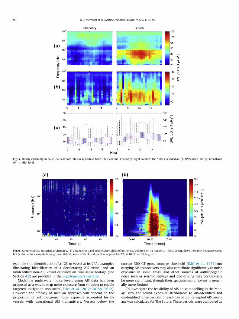
Fig. 5. Hourly variability in noise levels at both sites in 1/3 octave bands. Left column: Chanonry; Right column: The Sutors. (a) Median, (b) RMS mean, and (c) broadband(0.1–1 kHz) level.

Fig. 6. Sample spectra recorded at Chanonry. (a) Vocalisations and echolocation clicks of bottlenose dolphins on 12 August at 17:50. Spectra have the same frequency rangebut (a) has a finer amplitude range; and (b) oil tanker with closest point of approach (CPA) at 04:30 on 18 August.

90 N.D. Merchant et al. / Marine Pollution Bulletin 78 (2014) 85–95

example ship identification of a 125-m vessel at its CPA; examplesillustrating identification of a decelerating AIS vessel and anunidentified non-AIS vessel captured on time-lapse footage (seeSection 4.2) are provided in the Supplementary material.

Modelling underwater noise levels using AIS data has beenproposed as a way to map noise exposure from shipping to enabletargeted mitigation measures (Erbe et al., 2012; NOAA, 2012).However, the efficacy of such an approach will depend on theproportion of anthropogenic noise exposure accounted for byvessels with operational AIS transmitters. Vessels below the

current 300 GT gross tonnage threshold (IMO et al., 1974) notcarrying AIS transceivers may also contribute significantly to noiseexposure in some areas, and other sources of anthropogenicnoise such as seismic surveys and pile driving may occasionallybe more significant, though their spatiotemporal extent is gener-ally more limited.

To investigate the feasibility of AIS noise modelling in the Mor-ay Firth, the sound exposure attributable to AIS-identified andunidentified noise periods for each day of uninterrupted AIS cover-age was calculated for The Sutors. These periods were computed as

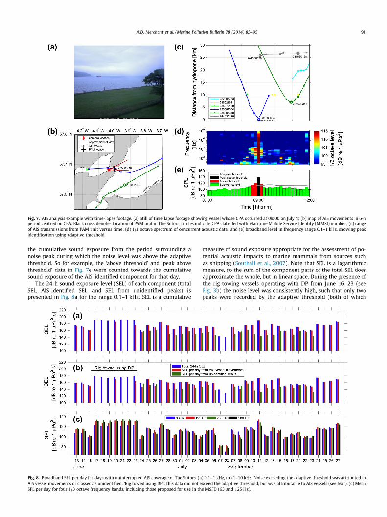
Fig. 7. AIS analysis example with time-lapse footage. (a) Still of time lapse footage showing vessel whose CPA occurred at 09:00 on July 4; (b) map of AIS movements in 6-hperiod centred on CPA. Black cross denotes location of PAM unit in The Sutors, circles indicate CPAs labelled with Maritime Mobile Service Identity (MMSI) number; (c) rangeof AIS transmissions from PAM unit versus time; (d) 1/3 octave spectrum of concurrent acoustic data; and (e) broadband level in frequency range 0.1–1 kHz, showing peakidentification using adaptive threshold.

N.D. Merchant et al. / Marine Pollution Bulletin 78 (2014) 85–95 91

the cumulative sound exposure from the period surrounding anoise peak during which the noise level was above the adaptivethreshold. So for example, the ‘above threshold’ and ‘peak abovethreshold’ data in Fig. 7e were counted towards the cumulativesound exposure of the AIS-identified component for that day.

The 24-h sound exposure level (SEL) of each component (totalSEL, AIS-identified SEL, and SEL from unidentified peaks) ispresented in Fig. 8a for the range 0.1–1 kHz. SEL is a cumulative

Fig. 8. Broadband SEL per day for days with uninterrupted AIS coverage of The Sutors. (aAIS vessel movements or classed as unidentified. ‘Rig towed using DP’: this data did not eSPL per day for four 1/3 octave frequency bands, including those proposed for use in th

measure of sound exposure appropriate for the assessment of po-tential acoustic impacts to marine mammals from sources suchas shipping (Southall et al., 2007). Note that SEL is a logarithmicmeasure, so the sum of the component parts of the total SEL doesapproximate the whole, but in linear space. During the presence ofthe rig-towing vessels operating with DP from June 16–23 (seeFig. 3b) the noise level was consistently high, such that only twopeaks were recorded by the adaptive threshold (both of which

) 0.1–1 kHz, (b) 1–10 kHz. Noise exceeding the adaptive threshold was attributed toxceed the adaptive threshold, but was attributable to AIS vessels (see text). (c) Meane MSFD (63 and 125 Hz).

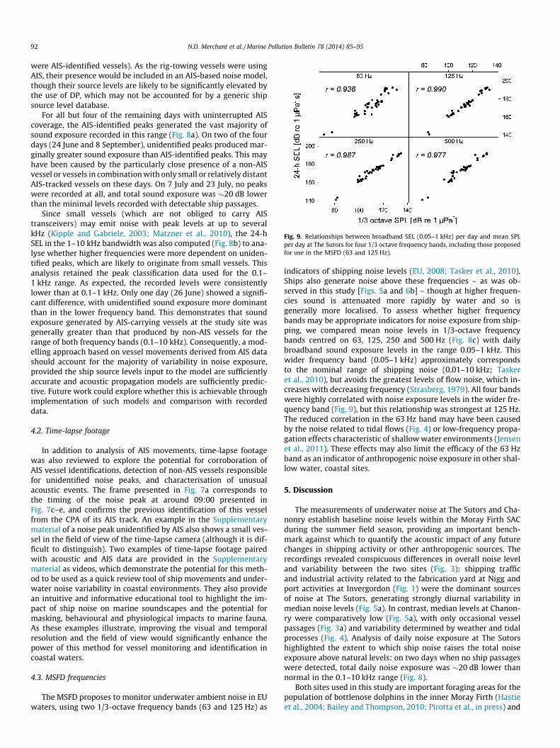
Fig. 9. Relationships between broadband SEL (0.05–1 kHz) per day and mean SPLper day at The Sutors for four 1/3 octave frequency bands, including those proposedfor use in the MSFD (63 and 125 Hz).

92 N.D. Merchant et al. / Marine Pollution Bulletin 78 (2014) 85–95

were AIS-identified vessels). As the rig-towing vessels were usingAIS, their presence would be included in an AIS-based noise model,though their source levels are likely to be significantly elevated bythe use of DP, which may not be accounted for by a generic shipsource level database.

For all but four of the remaining days with uninterrupted AIScoverage, the AIS-identified peaks generated the vast majority ofsound exposure recorded in this range (Fig. 8a). On two of the fourdays (24 June and 8 September), unidentified peaks produced mar-ginally greater sound exposure than AIS-identified peaks. This mayhave been caused by the particularly close presence of a non-AISvessel or vessels in combination with only small or relatively distantAIS-tracked vessels on these days. On 7 July and 23 July, no peakswere recorded at all, and total sound exposure was �20 dB lowerthan the minimal levels recorded with detectable ship passages.

Since small vessels (which are not obliged to carry AIStransceivers) may emit noise with peak levels at up to severalkHz (Kipple and Gabriele, 2003; Matzner et al., 2010), the 24-hSEL in the 1–10 kHz bandwidth was also computed (Fig. 8b) to ana-lyse whether higher frequencies were more dependent on uniden-tified peaks, which are likely to originate from small vessels. Thisanalysis retained the peak classification data used for the 0.1–1 kHz range. As expected, the recorded levels were consistentlylower than at 0.1–1 kHz. Only one day (26 June) showed a signifi-cant difference, with unidentified sound exposure more dominantthan in the lower frequency band. This demonstrates that soundexposure generated by AIS-carrying vessels at the study site wasgenerally greater than that produced by non-AIS vessels for therange of both frequency bands (0.1–10 kHz). Consequently, a mod-elling approach based on vessel movements derived from AIS datashould account for the majority of variability in noise exposure,provided the ship source levels input to the model are sufficientlyaccurate and acoustic propagation models are sufficiently predic-tive. Future work could explore whether this is achievable throughimplementation of such models and comparison with recordeddata.

4.2. Time-lapse footage

In addition to analysis of AIS movements, time-lapse footagewas also reviewed to explore the potential for corroboration ofAIS vessel identifications, detection of non-AIS vessels responsiblefor unidentified noise peaks, and characterisation of unusualacoustic events. The frame presented in Fig. 7a corresponds tothe timing of the noise peak at around 09:00 presented inFig. 7c–e, and confirms the previous identification of this vesselfrom the CPA of its AIS track. An example in the Supplementarymaterial of a noise peak unidentified by AIS also shows a small ves-sel in the field of view of the time-lapse camera (although it is dif-ficult to distinguish). Two examples of time-lapse footage pairedwith acoustic and AIS data are provided in the Supplementarymaterial as videos, which demonstrate the potential for this meth-od to be used as a quick review tool of ship movements and under-water noise variability in coastal environments. They also providean intuitive and informative educational tool to highlight the im-pact of ship noise on marine soundscapes and the potential formasking, behavioural and physiological impacts to marine fauna.As these examples illustrate, improving the visual and temporalresolution and the field of view would significantly enhance thepower of this method for vessel monitoring and identification incoastal waters.

4.3. MSFD frequencies

The MSFD proposes to monitor underwater ambient noise in EUwaters, using two 1/3-octave frequency bands (63 and 125 Hz) as

indicators of shipping noise levels (EU, 2008; Tasker et al., 2010).Ships also generate noise above these frequencies – as was ob-served in this study [Figs. 5a and 6b] – though at higher frequen-cies sound is attenuated more rapidly by water and so isgenerally more localised. To assess whether higher frequencybands may be appropriate indicators for noise exposure from ship-ping, we compared mean noise levels in 1/3-octave frequencybands centred on 63, 125, 250 and 500 Hz (Fig. 8c) with dailybroadband sound exposure levels in the range 0.05–1 kHz. Thiswider frequency band (0.05–1 kHz) approximately correspondsto the nominal range of shipping noise (0.01–10 kHz; Taskeret al., 2010), but avoids the greatest levels of flow noise, which in-creases with decreasing frequency (Strasberg, 1979). All four bandswere highly correlated with noise exposure levels in the wider fre-quency band (Fig. 9), but this relationship was strongest at 125 Hz.The reduced correlation in the 63 Hz band may have been causedby the noise related to tidal flows (Fig. 4) or low-frequency propa-gation effects characteristic of shallow water environments (Jensenet al., 2011). These effects may also limit the efficacy of the 63 Hzband as an indicator of anthropogenic noise exposure in other shal-low water, coastal sites.

5. Discussion

The measurements of underwater noise at The Sutors and Cha-nonry establish baseline noise levels within the Moray Firth SACduring the summer field season, providing an important bench-mark against which to quantify the acoustic impact of any futurechanges in shipping activity or other anthropogenic sources. Therecordings revealed conspicuous differences in overall noise leveland variability between the two sites (Fig. 3): shipping trafficand industrial activity related to the fabrication yard at Nigg andport activities at Invergordon (Fig. 1) were the dominant sourcesof noise at The Sutors, generating strongly diurnal variability inmedian noise levels (Fig. 5a). In contrast, median levels at Chanon-ry were comparatively low (Fig. 5a), with only occasional vesselpassages (Fig. 3a) and variability determined by weather and tidalprocesses (Fig. 4). Analysis of daily noise exposure at The Sutorshighlighted the extent to which ship noise raises the total noiseexposure above natural levels: on two days when no ship passageswere detected, total daily noise exposure was �20 dB lower thannormal in the 0.1–10 kHz range (Fig. 8).

Both sites used in this study are important foraging areas for thepopulation of bottlenose dolphins in the inner Moray Firth (Hastieet al., 2004; Bailey and Thompson, 2010; Pirotta et al., in press) and

N.D. Merchant et al. / Marine Pollution Bulletin 78 (2014) 85–95 93

dolphins were confirmed to use them regularly throughout thedeployment periods. Since the population appears to be stable orincreasing (Cheney et al., 2013), the current noise levels we presentare not expected to pose a threat to dolphin population levels. Nev-ertheless, the difference in baseline soundscape between the twoforaging areas could influence how these sites may be affectedby any future increases in shipping noise. While The Sutors is cur-rently expected to experience greater increases in traffic associatedwith offshore energy developments, dolphins may already beaccustomed to higher noise levels in this area. On the other hand,Chanonry is currently much quieter, meaning that a smaller in-crease in shipping noise could result in a greater degradation ofhabitat quality.

Analysis of noise levels at The Sutors in conjunction with AISship-tracking data demonstrated that the majority of total soundexposure at the site was attributable to vessels operating withAIS transceivers (Fig. 8). This indicates that modelling of noise lev-els based on AIS-vessel movements (e.g. Erbe et al., 2012; Bassettet al., 2012) should account for most of the noise exposureobserved experimentally, provided other model parameters (shipsource levels, acoustic propagation loss profiles) are sufficientlyaccurate. This result suggests that models based on plannedincreases in vessel movements in the Moray Firth (Lusseau et al.,2011; New et al., 2013) may be able to forecast associatedincreases in noise exposure, and is a promising indication thatAIS-based noise mapping could be successfully applied to targetship noise mitigation efforts in other marine habitats. However,caution should be exercised in extrapolating from this result sincein areas further from commercial shipping activity, the dominantsource of ship noise may be smaller craft not operating with AIStransceivers.

This study also introduces the pairing of shore-based time-lapsefootage with acoustic and AIS data as a tool for monitoring theinfluence of human activities on coastal marine soundscapes. Themethod enabled identification of abnormally loud events such asrigs being towed past the deployment site, and facilitated detec-tion of non-AIS vessels responsible for noise peaks and corrobora-tion of AIS-based vessel identification (Fig. 7). With improvedresolution and field of view, time-lapse monitoring could facilitatemore detailed characterisation of non-AIS vessel traffic in coastalareas, enhancing understanding of the relative importance of smallvessels to marine noise pollution.

Comparison of spectra documenting bottlenose dolphin vocali-sations and a ship passage at Chanonry (Fig. 6) highlights the po-tential for vocalisation masking by transiting vessels.Odontocetes use echolocation to navigate and to find and capturefood (Au, 1993). Disruption to these activities caused by acousticmasking could thus affect energy acquisition and allocation, withlong-term implications for vital rates (New et al., 2013). A noisiersoundscape could also lead to degradation of the dolphin popula-tion’s habitat (Tyack, 2008) such as through effects on fish prey(Popper et al., 2003). Moreover, social interactions could be af-fected by vocalisation masking since sound is critical for communi-cation among conspecifics. Future work could investigate theextent to which the effective communication range – which hasbeen estimated for this population in the absence of vessels (Janik,2000) – is reduced by the presence of vessel noise (e.g. Erbe, 2002;Hatch et al., 2012; Williams et al., in press). A rise in noise fromship traffic could also induce anti-predatory behavioural responses(Tyack, 2008) and increase individual levels of chronic stress(Wright et al., 2007; Rolland et al., 2012). Research efforts shouldthus aim to characterise dolphin responses to ship noise in thisarea, and to understand whether increased ship traffic has the po-tential to alter the animals’ activity budget.

The study also highlighted some important issues for the imple-mentation of the European MSFD. Our measurements show that

low-frequency flow noise may dominate in areas of high tidal flow,potentially contaminating noise levels at 63 and 125 Hz – frequen-cies at which the current legislation proposes to monitor ambientnoise (EU, 2008; Dekeling et al., 2013). Flow noise is a form ofpseudo-noise caused by turbulence around the hydrophone (Stras-berg, 1979), and is not actually present in the environment. Whilenoise from shipping was more dominant than flow noise at bothsites (Fig. 5), flow noise exceeded non-anthropogenic noise levelsbelow �160 Hz at the Chanonry site (Fig. 4), and so may influencemeasurements in areas of low shipping density. Since flow noisedecreases with increasing frequency (Strasberg, 1979), higher fre-quency bands would be progressively less susceptible to flow noisecontamination than those at 63 and 125 Hz.

Comparison of the proposed 1/3-octave frequency bands withthose at 250 and 500 Hz (Fig. 9) indicates that the 250 Hz bandmay be as responsive to noise exposure from large vessels as the125 Hz band, and may perform better than the 63 Hz band in shal-low water. Although peak frequencies of commercial ship sourcelevels are typically <100 Hz (e.g. Arveson and Vendittis, 2000;McKenna et al., 2012), low-frequency sound may be rapidly atten-uated in shallow water depending on the water depth (Jensenet al., 2011), meaning received ship noise levels may have higherpeak frequencies than in the open ocean. The 250- and 500-Hzbands are also likely to contain a greater amount of the noise fromsmall vessels (since their spectra can peak at up to several kHz(Kipple and Gabriele, 2003; Matzner et al., 2010)), which may bethe dominant source of ship noise in some coastal areas. Inclusionof noise levels at frequencies greater than 125 Hz may therefore beparticularly informative for MSFD noise monitoring in shallowwaters.

A wider concern for the efficacy of the MSFD with regard toshipping noise is the proposed focus (Van der Graaf et al.,2012; Dekeling et al., 2013) of ambient noise monitoring on highshipping density areas. While it is important that the mostacoustically polluted waters are represented in noise monitoringprograms, it is arguably the case that habitats most at threatfrom anthropogenic pressure should be given greater weight. Ifnoise levels in high shipping areas are to determine whether amember state of the European Union attains ‘Good Environmen-tal Status’, there is a risk that more significant changes to themarine acoustic environment in less polluted areas will beoverlooked.

Acknowledgements

Funding for equipment and data collection was provided byMoray Offshore Renewables Ltd., and Beatrice Offshore Wind Ltd.We thank Baker Consultants and Moray First Marine for their assis-tance with device calibration and deployment, respectively. ThePOLPRED tidal model was kindly provided by NERC NationalOceanography Centre. We also thank Rebecca Hewitt for collatingand preparing the weather data, Stephanie Moore for advice onsediment transport, and Ian McConnell of shipais.com for AIS data.N.D.M. was funded by an EPSRC Doctoral Training Award (No. EP/P505399/1). E.P. was funded by the MASTS pooling initiative (TheMarine Alliance for Science and Technology for Scotland) and theirsupport is gratefully acknowledged. MASTS is funded by the Scot-tish Funding Council (Grant Reference HR09011) and contributinginstitutions.

Appendix A. Supplementary data

Supplementary data associated with this article can be found, inthe online version, at http://dx.doi.org/10.1016/j.marpolbul.2013.10.058.

94 N.D. Merchant et al. / Marine Pollution Bulletin 78 (2014) 85–95

References

Andrew, R.K., Howe, B.M., Mercer, J.A., Dzieciuch, M.A., 2002. Ocean ambient sound:Comparing the 1960s with the 1990s for a receiver off the California coast.Acoustics Research Letters Online 3 (2), 65–70.

Arveson, P.T., Vendittis, D.J., 2000. Radiated noise characteristics of a modern cargoship. Journal of the Acoustical Society of America 107 (1), 118–129.

Au, W.W., 1993. The Sonar of Dolphins. Springer, New York.Bailey, H., Thompson, P., 2010. Effect of oceanographic features on fine-scale

foraging movements of bottlenose dolphins. Marine Ecology Progress Series418, 223–233.

Bassett, C., Polagye, B., Holt, M., Thomson, J., 2012. A vessel noise budget forAdmiralty Inlet, Puget Sound, Washington (USA). Journal of the AcousticalSociety of America 132 (6), 3706–3719.

Bassett, C., Thomson, J., Polagye, B., 2013. Sediment-generated noise and bed stressin a tidal channel. Journal of Geophysical Research: Oceans 118 (4), 2249–2265.

Buckstaff, K.C., 2004. Effects of watercraft noise on the acoustic behavior ofbottlenose dolphins, Tursiops truncatus, in Sarasota Bay, Florida. MarineMammal Science 20 (4), 709–725.

Butler, J.R., Middlemas, S.J., McKelvey, S.A., McMyn, I., Leyshon, B., Walker, I.,Thompson, P.M., Boyd, I.L., Duck, C., Armstrong, J.D., 2008. The Moray Firth SealManagement Plan: an adaptive framework for balancing the conservation ofseals, salmon, fisheries and wildlife tourism in the UK. Aquatic Conservation:Marine and Freshwater Ecosystems 18 (6), 1025–1038.

Chapman, N.R., Price, A., 2011. Low frequency deep ocean ambient noise trend inthe Northeast Pacific Ocean. Journal of the Acoustical Society of America 129(5), EL161–EL165.

Cheney, B., Thompson, P.M., Ingram, S.N., Hammond, P.S., Stevick, P.T., Durban, J.W.,Culloch, R.M., Elwen, S.H., Mandleberg, L., Janik, V.M., Quick, N.J., Islas-Villanueva, V., Robinson, K.P., Costa, M., Eisfeld, S.M., Walters, A., Phillips, C.,Weir, C.R., Evans, P.G.H., Anderwald, P., Reid, R.J., Reid, J.B., Wilson, B., 2013.Integrating multiple data sources to assess the distribution and abundance ofbottlenose dolphins Tursiops truncatus in Scottish waters. Mammal Review 43(1), 71–88.

Christiansen, F., Lusseau, D., Stensland, E., Berggren, P., 2010. Effects of tourist boatson the behaviour of Indo-Pacific bottlenose dolphins off the south coast ofZanzibar. Endangered Species Research 11 (1), 91–99.

Clark, C.W., Ellison, W.T., Southall, B.L., Hatch, L., Van Parijs, S.M., Frankel, A.,Ponirakis, D., 2009. Acoustic masking in marine ecosystems: intuitions,analysis, and implication. Marine Ecology Progress Series 395, 201–222.

Dekeling, R., Tasker, M., Ainslie, M., Andersson, M., André, M., Castellote, M., Borsani,J., Dalen, J., Folegot, T., Leaper, R., Liebschner, A., Pajala, J., Robinson, S., Sigray, P.,Sutton, G., Thomsen, F., Van der Graaf, A., Werner, S., Wittekind, D., Young, J.2013. Monitoring Guidance for Underwater Noise in European Seas – 2ndReport of the Technical Subgroup on Underwater noise (TSG Noise). InterimGuidance Report., Tech. Rep. <http://www.dredging.org/documents/ceda/downloads/msfd_monitoring_guidance_underwater_noise_part_i_summary_recommendations_igr_0516.pdf>.

Ellison, W.T., Southall, B.L., Clark, C.W., Frankel, A.S., 2012. A new context-basedapproach to assess marine mammal behavioral responses to anthropogenicsounds. Conservation Biology 26 (1), 21–28.

Erbe, C., 2002. Underwater noise of whale-watching boats and potential effects onkiller whales (Orcinus orca), based on an acoustic impact model. MarineMammal Science 18 (2), 394–418.

Erbe, C., MacGillivray, A., Williams, R., 2012. Mapping cumulative noise fromshipping to inform marine spatial planning. Journal of the Acoustical Society ofAmerica 132 (5), EL423–EL428.

EU, 2008. Directive 2008/56/EC of the European Parliament and of the Council of 17June 2008, establishing a framework for community action in the field ofmarine environmental policy (Marine Strategy Framework Directive). OfficialJournal of the European Union L164, 19–40.

Foote, A.D., Osborne, R.W., Hoelzel, A.R., 2004. Whale-call response to masking boatnoise. Nature 428 (6986), 910.

Frisk, G., 2012. Noiseonomics: the relationship between ambient noise levels in thesea and global economic trends. Scientific Reports 2 (437).

Hastie, G.D., Wilson, B., Wilson, L., Parsons, K., Thompson, P., 2004. Functionalmechanisms underlying cetacean distribution patterns: hotspots for bottlenosedolphins are linked to foraging. Marine Biology 144 (2), 397–403.

Hatch, L.T., Clark, C.W., Van Parijs, S.M., Frankel, A.S., Ponirakis, D.W., 2012.Quantifying loss of acoustic communication space for right whales in andaround a US National Marine Sanctuary. Conservation Biology 26 (6), 983–994.

Heide-Jørgensen, M.P., Hansen, R.G., Westdal, K., Reeves, R.R., Mosbech, A., 2013.Narwhals and seismic exploration: is seismic noise increasing the risk of iceentrapments? Biological Conservation 158, 50–54.

Hildebrand, J.A., 2009. Anthropogenic and natural sources of ambient noise in theocean. Marine Ecology Progress Series 395, 5–20.

IMO, 2000. International convention for the Safety of Life at Sea (SOLAS), Chapter VSafety of Navigation, Regulation, vol. 19 (first ed., 1974, amended December2000).

Janik, V.M., 2000. Source levels and the estimated active space of bottlenose dolphin(Tursiops truncatus) whistles in the Moray Firth, Scotland. Journal ofComparative Physiology A 186 (7–8), 673–680.

Jensen, F.H., Bejder, L., Wahlberg, M., Soto, N.A., Johnson, M., Madsen, P.T., 2009.Vessel noise effects on delphinid communication. Marine Ecology ProgressSeries 395, 161–175.

Jensen, F.B., Kuperman, W.A., Porter, M.B., Schmidt, H., 2011. Computational OceanAcoustics. Springer, New York.

Kewley, D.J., 1990. Low-frequency wind-generated ambient noise source levels.Journal of the Acoustical Society of America 88 (4), 1894–1902.

Kipple, B., Gabriele, C., 2003. Glacier Bay watercraft noise, NSWC Technical ReportNSWCCD-71-TR-2003/522. <http://www.nps.gov/glba/naturescience/upload/GBWatercraftNoiseRpt.pdf>.

Lusseau, D., 2003. Effects of tour boats on the behavior of bottlenose dolphins: usingMarkov chains to model anthropogenic impacts. Conservation Biology 17 (6),1785–1793.

Lusseau, D., New, L., Donovan, C., Cheney, B., Thompson, P., Hastie, G., Harwood, J.2011. The development of a framework to understand and predict thepopulation consequences of disturbances for the Moray Firth bottlenosedolphin population, Tech. Rep., Scottish Natural Heritage. CommissionedReport No. 468, Scottish Natural Heritage, Perth UK.

Ma, B.B., Nystuen, J.A., 2005. Passive acoustic detection and measurement of rainfallat sea. Journal of Atmospheric and Oceanic Technology 22 (8), 1225–1248.

Matzner, S., Maxwell, A., Myers, J., Caviggia, K., Elster, J., Foley, M., Jones, M., Ogden,G., Sorensen, E., Zurk, L., Tagestad, J., Stephan, A., Peterson, M., Bradley, D., 2010.Small vessel contribution to underwater noise. In: OCEANS 2010. IEEE.

McDonald, M.A., Hildebrand, J.A., Wiggins, S.M., 2006. Increases in deep oceanambient noise in the northeast pacific west of San Nicolas Island, California.Journal of the Acoustical Society of America 120 (2), 711–718.

McKenna, M.F., Ross, D., Wiggins, S.M., Hildebrand, J.A., 2012. Underwater radiatednoise from modern commercial ships. Journal of the Acoustical Society ofAmerica 131 (1), 92–103.

Merchant, N.D., Blondel, P., Dakin, D.T., Dorocicz, J., 2012a. Averaging underwaternoise levels for environmental assessment of shipping. Journal of the AcousticalSociety of America 132 (4), EL343–EL349.

Merchant, N.D., Witt, M.J., Blondel, P., Godley, B.J., Smith, G.H., 2012b. Assessingsound exposure from shipping in coastal waters using a single hydrophone andAutomatic Identification System (AIS) data. Marine Pollution Bulletin 64 (7),1320–1329.

Merchant, N.D., Barton, T.R., Thompson, P.M., Pirotta, E., Dakin, D.T., Dorocicz, J.,2013. Spectral probability density as a tool for ambient noise analysis. Journal ofthe Acoustical Society of America 133 (4), EL262–EL267.

Moore, S.E., Stafford, K.M., Melling, H., Berchok, C., Wiig, O., Kovacs, K.M., Lydersen,C., Richter-Menge, J., 2012. Comparing marine mammal acoustic habitats inAtlantic and Pacific sectors of the High Arctic: year-long records from FramStrait and the Chukchi Plateau. Polar Biology 35 (3), 475–480.

National Research Council, 2005. Marine Mammal Populations and Ocean Noise:Determining when Noise Causes Biologically Significant Effects, NationalAcademies Press, Washington, DC.

New, L.F., Harwood, J., Thomas, L., Donovan, C., Clark, J.S., Hastie, G., Thompson, P.M.,Cheney, B., Scott-Hayward, L., Lusseau, D., 2013. Modelling the biologicalsignificance of behavioural change in coastal bottlenose dolphins in response todisturbance. Functional Ecology 27 (2), 314–322.

NOAA, 2012. CetSound project. <http://cetsound.noaa.gov/index.html> (lastaccessed 27.10.13).

Nowacek, D.P., Thorne, L.H., Johnston, D.W., Tyack, P.L., 2007. Responses ofcetaceans to anthropogenic noise. Mammal Review 37 (2), 81–115.

Parks, S.E., Clark, C.W., Tyack, P.L., 2007. Short- and long-term changes in rightwhale calling behavior: the potential effects of noise on acousticcommunication. Journal of the Acoustical Society of America 122 (6), 3725–3731.

Pirotta, E., Thompson, P., Miller, P., Brookes, K., Cheney, B., Barton, T., Graham, I.,Lusseau, D. in press. Scale-dependent foraging ecology of a marine top predatormodelled using passive acoustic data, Functional Ecology. <http://dx.doi.org/10.1111/1365-2435.12146>.

Popper, A.N., Fewtrell, J., Smith, M.E., McCauley, R.D., 2003. Anthropogenic sound:effects on the behavior and physiology of fishes. Marine Technology SocietyJournal 37 (4), 35–40.

Reid, J.B., Evans, P.G., Northridge, S.P. 2003. Atlas of cetacean distribution in north-west European waters, Joint Nature Conservation Committee, Peterborough,UK.

Richardson, W.J., Greene, C.R., Malme, C.I., Thompson, D.H., 1995. Marine Mammalsand Noise. Academic Press, San Diego, USA.

Rolland, R.M., Parks, S.E., Hunt, K.E., Castellote, M., Corkeron, P.J., Nowacek, D.P.,Wasser, S.K., Kraus, S.D., 2012. Evidence that ship noise increases stress in rightwhales. Proceedings of the Royal Society B: Biological Sciences 279 (1737),2363–2368.

Scottish Government, 2011. 2020 Routemap for renewable energy in Scotland,Scottish Government, Edinburgh, UK. <http://www.scotland.gov.uk/Resource/Doc/917/0118802.pdf>.

Širovic, A., Wiggins, S.M., Oleson, E.M., 2013. Ocean noise in the tropical andsubtropical Pacific Ocean. Journal of the Acoustical Society of America 134 (4),2681–2689.

Southall, B.L., Bowles, A.E., Ellison, W.T., Finneran, J.J., Gentry, R.L., Greene, J.,Charles, R., Kastak, D., Ketten, D.R., Miller, J.H., Nachtigall, P.E., Richardson, W.J.,Thomas, J.A., Tyack, P.L., 2007. Marine mammal noise exposure criteria: Initialscientific recommendations. Aquatic Mammals 33 (4), 411–521.

Strasberg, M., 1979. Nonacoustic noise interference in measurements of infrasonicambient noise. Journal of the Acoustical Society of America 66 (5), 1487–1493.

Tasker, M., Amundin, M., André, M., Hawkins, A., Lang, W., Merck, T., Scholik-Schlomer, A., Teilmann, J., Thomsen, F., Werner, S., Zakharia, M., 2010. MarineStrategy Framework Directive G Task Group 11 Report Underwater noise and

N.D. Merchant et al. / Marine Pollution Bulletin 78 (2014) 85–95 95

other forms of energy, EUR 24341 EN G Joint Research Centre, Luxembourg:Office for Official Publications of the European Communities, 55pp.

Thorne, P.D., 1986. Laboratory and marine measurements on the acoustic detectionof sediment transport. Journal of the Acoustical Society of America 80 (3), 899–910.

Tyack, P.L., 2008. Implications for marine mammals of large-scale changes in themarine acoustic environment. Journal of Mammalogy 89 (3), 549–558.

Van der Graaf, A., Ainslie, M.A., Andre, M., Brensing, K., Dalen, J., Dekeling, R.,Robinson, S., Tasker, M., Thomsen, F., Werner, S. 2012. European Marine StrategyFramework Directive – Good Environmental Status (MSFD GES): Report of theTechnical Subgroup on Underwater Noise and Other Forms of Energy. <http://ec.europa.eu/environment/marine/pdf/MSFD_reportTSG_Noise.pdf>.

Welch, P., 1967. The use of fast Fourier transform for the estimation of powerspectra: a method based on time averaging over short, modified periodograms.IEEE Transactions on Audio and Electroacoustics 15 (2), 70–73.

Wenz, G.M., 1962. Acoustic ambient noise in the ocean: spectra and sources. Journalof the Acoustical Society of America 34 (12), 1936–1956.

Williams, R., Trites, A.W., Bain, D.E., 2002. Behavioural responses of killer whales(Orcinus orca) to whale-watching boats: opportunistic observations andexperimental approaches. Journal of Zoology 256 (2), 255–270.

Williams, R., Clark, C.W., Ponirakis, D., Ashe, E., in press. Acoustic quality of criticalhabitats for three threatened whale populations, Animal Conservation. <http://dx.doi.org/10.1111/acv.12076>.

Wright, A.J., Soto, N.A., Baldwin, A.L., Bateson, M., Beale, C.M., Clark, C., Deak, T.,Edwards, E.F., Fernndez, A., Godinho, A., Hatch, L.T., Kakuschke, A., Lusseau, D.,Martineau, D., Romero, M.L., Weilgart, L.S., Wintle, B.A., Notarbartolo-di Sciara,G., Martin, V., 2007. Do marine mammals experience stress related toanthropogenic noise? International Journal of Comparative Psychology 20 (2),274–316.