monocular visual mapping with the fast hough transformnwerneck.sdf.org/almoxarifado/72827.pdfand is...

Monocular visual mapping with the Fast Hough Transform

Nicolau Leal Werneck and Anna Helena Reali Costa

[email protected], [email protected]

Intelligent Techniques Laboratory (LTI) — PCS — USP

Av. Prof. Luciano Gualberto tv. 3, 158

05508-900 Sao Paulo, SP, Brazil

Abstract

This article presents a mapping algorithm for bearing-

only sensors, largely based on the Fast Hough Transform.

While just the specific case of a camera moving in a straight

path and detecting orthogonal edges was considered, the

principle should be useful for more complex scenarios too.

The algorithm is intended for creating initial estimates of

landmark positions to allow the application of other classic

mapping methods, such as maximum likelihood bundle ad-

justment. Tests were conducted with a video obtained with a

consumer camcorder moving through a corridor, and good

initial estimates were successfully generated.

1. Introduction

The goal of simultaneous localization and map-

ping (SLAM) [14, 4] with visual sensors, or visual SLAM,

is to produce estimates of both the location of a cam-

era over time and of visual landmarks such as points and

edges perceived by the camera [10, 3, 5, 1, 8, 19]. It is

closely related to the Computer Vision problem of struc-

ture from motion (SFM) [13], more specifically to the

bundle adjustment (BA) problem [16], which is the prob-

lem of estimating model parameters of both the structure of

a scene and the camera used to produce images from it, op-

timizing the reconstruction of the set of images. The

main difference is that in SLAM problems there is of-

ten some kind of motion information available, and there is

also the desire to operate in real-time.

Visual SLAM has been usually done with filtering tech-

niques from Mobile Robotics, such as the Extended Kalman

Filter [3], but there is a growing desire in the research com-

munity to change the focus towards algorithms that are

more similar to the global optimization techniques that have

become the standard for BA [13]. The present article con-

tributes to this by proposing a map building algorithm based

on the Fast Hough Transform (FHT) [9] to create initial map

estimates when little information about the environment is

available, and feed other algorithms to finish the SLAM pro-

cess. The execution of the algorithm depends on a couple of

parameters that should in principle be easily found for spe-

cific applications by the observation of some statistics de-

scribed in the article. The algorithm successfully located a

few points in tests performed with a video recorded with

a camera moving down a hallway, and seems to be a good

match for more accurate SLAM systems that require initial

map estimates. The points were also found to be good so-

lution estimates, not being much improved by the use of a

maximum likelihood (ML) algorithm [17].

The Hough Transform (HT) is a well-known technique to

locate straight lines and other objects in digital images [6].

Many modifications to the original algorithm were proposed

in the last decades, most of them looking for alternatives

that are either faster or consume less memory. The basic

idea is to create a large array of accumulators that are in-

cremented following lines (or other curves) with param-

eters defined by each point of the image. The resolution

of this transform space is determined a priori, and is di-

rectly related to the precision of the results and the com-

putational cost. Many HT implementations actually create

all these accumulator in memory. In the Fast Hough Trans-

form a coarse-to-fine search strategy is adopted instead. A

quadtree is created by recursively splitting the transform

space in cells where the count of crossing lines surpasses

a minimum value [9]. This strategy seeks to focus the pro-

cessing inside regions where the peaks are most likely to

be found. Another proposal that has a similar coarse-to-fine

strategy is the Adaptive Hough Transform, but it is not able

to find multiple peaks at the same time [6].

The use of Hough transform techniques to perform map-

ping in monocular vision is justified by noting how the prob-

lem can become one of finding the parameters of a set of

lines from where points, related to the observations, were

sampled [18, 17]. The Hough transform is also known to be

an approximation to the maximum likelihood method [12],

what is a more theoretically sound and popular approach,

04-07 de Julho - FCT/UNESP - P. Prudente VI Workshop de Visão Computacional

279

and is used for BA.

The BA problem is usually approached in two steps. First

the evidences must be assigned to each model parameter,

what constitutes the correspondence problem. Then the val-

ues of the parameters must be calculated, what is usually

done with some sort of ML technique. In traditional BA,

where no kind of motion information is available, the most

applied technique is RANSAC, where correspondences are

assigned randomly, and the ones that result in a good agree-

ment are kept [2, 15]. RANSAC is very traditional, but the

original concept can be improved in many ways. More so-

phisticated heuristics can also be used if the problem is re-

garded in the framework of convex programming [7]. In

the filtering approach to visual SLAM the correspondences

are assigned at each frame to the landmark with the closest

projection, and then the landmarks are updated iteratively,

with one new evidence every frame [3, 5, 11]. The tech-

nique studied here differs from the filtering approach be-

cause multiple images are considered at the same time, and

differs from the basic RANSAC approach because there is

motion information available to explore.

The next section of this article will present the proposed

algorithm. Section 3 describes the results of applying the al-

gorithm to data extracted from a film recorded on a hallway.

Finally, the last section brings a few conclusions.

2. The proposed algorithm

This section first explains why and how the FHT might

be a good alternative for map building with visual sensors,

then describe some interesting phenomena observed in do-

ing so. This leads to a discussion about how to set the pa-

rameters of the FHT algorithm in the present scenario.

2.1. Justification

While in principle the technique presented here could be

used in problems with many degrees of freedom, only the

case of straight paths are being considered. The detected vi-

sual landmarks are also edges found by a simple analysis

over a central line or column of the images. It can be shown

that in these conditions the inverse of the image coordinates

have a linear relationship with the camera position [18, 17].

Therefore building a map of this environment becomes the

problem of fitting straight lines to the set of points collected,

provided the location of the camera is known at each step,

and the inverse coordinates are calculated. Figure 1 shows a

frame from the film used in the experiments reported in this

paper. The vertical edges from the columns, doors and win-

dows are the landmarks being sought. It must be clear to the

reader that the Hough Transform is not being used here to

locate these edges in the images, but to find their space co-

ordinates given the image coordinates in a sequence of im-

ages.

Figure 1. Example frame from corridor se-quence.

When the HT is used to find the parameters of the lines

in an image, lines corresponding to each point are drawn in

the parameter space, following the so-called line-point du-

ality. The parameters for the line in the original space are

given by the point in the transform space where the lines

meet. But this is exactly what happens in mapping with vi-

sual sensors, or bearings-only sensors in general: the obser-

vations define lines in the space, and we wish to find the

points where these lines meet, as Figure 2 shows. Therefore

Hough transform techniques developed to find these meet-

ing points from line sets should be applicable to the visual

mapping problem. All it takes is to treat the space where

the camera is moving as the parameter space in the Hough

transform where we look for the meeting points of the sets

of lines, which are related to the observations.

One advantage of using the FHT algorithm is that there is

no need to determinate a priori the resolution of the param-

eter space, although the best results were found by stopping

the algorithm when a minimum resolution selected prior to

the run was reached. Another advantage is that it does not

need the information of the correspondences between the

observation and landmarks, and starts from no knowledge

of the number or location of the landmarks. At the end of

the processing a set of landmarks estimates is produced, that

can be further analyzed and refined by other algorithms.

2.2. Adaptation to the problem

The algorithm starts analyzing a large square, that is the

root of the quadtree. The landmarks and camera positions

are determined by a pair of coordinates: a longitudinal co-

ordinate in the direction of the camera track, and a lateral


280

Figure 2. Camera path, landmarks and detec-

tions in a visual SLAM problem. The lines

related to each detection meet at the land-marks. Figure reproduced from [17].

coordinate on the axis orthogonal to this track. Because of

the straight motion, camera positions always have the lat-

eral coordinate set to zero. Assuming uniform motion, the

distance between the successive camera positions can also

be normalized to one, turning the camera coordinates into

the sequence of natural numbers.

Landmarks at the left or right of the path, with positive

and negative lateral coordinates, can be analyzed separately,

splitting the problem into the analysis of each side of the

images at a time. Doing that allows the basis of the initial

quadree square to be made congruent to the path of the cam-

era, since observations will reside only in one side of the

path. One side of the square can also be made to cross the

position of the first image in the series, since the camera has

a limited and forward-pointing field of view, and no obser-

vations will produce lines that go behind that point. In the

present work there was no calculation of an optimal posi-

tion for the other sides, or for the initial size of the square,

and the value used was simply a large enough one.

At each iteration of the algorithm the lines relative to

each observation are tested to see if they cross each cell in

the leaves of the quadtree. The lines start from the longitu-

dinal axis at the point corresponding to the position of the

camera where that feature was detected, and extends indef-

initely from there at the angle corresponding to the image

position of the detected feature. It is important to remem-

ber here that the actual focal distance value was not used or

even measured, being replaced by a normalized value. The

result of using an artificial focal distance value is that the

map is not isotropic, and correct only up to two scale fac-

tors. To obtain a correct map we need to know both the cor-

rect focal distance, and also the correct distances between

the camera positions.

The number of crossing lines are counted for each cell,

and if a threshold value is attained, that cell is divided into

other 4 cells, one for each quadrant. This counting thresh-

old is a parameter for the algorithm, and no attempt to cal-

culate an optimal value was made yet. The calculation of a

good value must depend both on the precision of the obser-

vations and on the number of detections a typical landmark

should produce, which is indirectly related to the length be-

tween the cameras, the field of view angle and the distance

of the camera to the landmarks.

The search was stopped when a maximum resolution was

found. The value used in the final version of the algorithm

was a square of unit length, where the unit is also the sup-

posed distance between successive frames of the film. The

final squares with a count above the threshold are the solu-

tions. Figure 3 shows a solution found in a test, and a de-

tailed view of one region with cells in the highest resolu-

tion.

If the data were perfect, the lines should all meet at a

single point, but imperfections and uncertainties move the

lines, turning the meeting points into regions of high den-

sity of lines. A final processing step was therefore intro-

duced. The set of cells found in the previous step are made

into pixels of a binary image. This image was then pro-

cessed with the morphological dilation operation, and the

centroids of the resulting connected components constitute

the final landmark proposals. The dilation was applied to

group together connected components that were separated

by just a thin line of pixels, turning them into a single land-

mark estimate. The detailed view in Figure 3 shows a sin-

gle cell separated from the larger cluster by another cell,

what is a good example of why the dilation should be ap-

plied. This might be replaced by other procedures that take

into account the uncertainties to group separate pairs of es-

timates into a single one or not.

One last but important detail of the current implementa-

tion is that instead of using all observations, only the obser-

vations closest to the edge of the frame were considered at

each image half analyzed. The use of the complete set of ob-

servations was left to the next step inside the complete lo-

calization and mapping procedure.

2.3. Convergence dynamics

When the algorithm starts we have a single cell that has

a count equal to the total number of observations. As the al-

gorithm progresses, the number of cells increase, at most in

an exponential rate, with 4n cells at the n-th step. What was

found in experiments is that an exponential rate is in fact

found for the first steps, but usually with a basis between 3

and 4. This happens until a peak value is reached. After the

peak, the number of cells starts to decrease as the resolu-


281

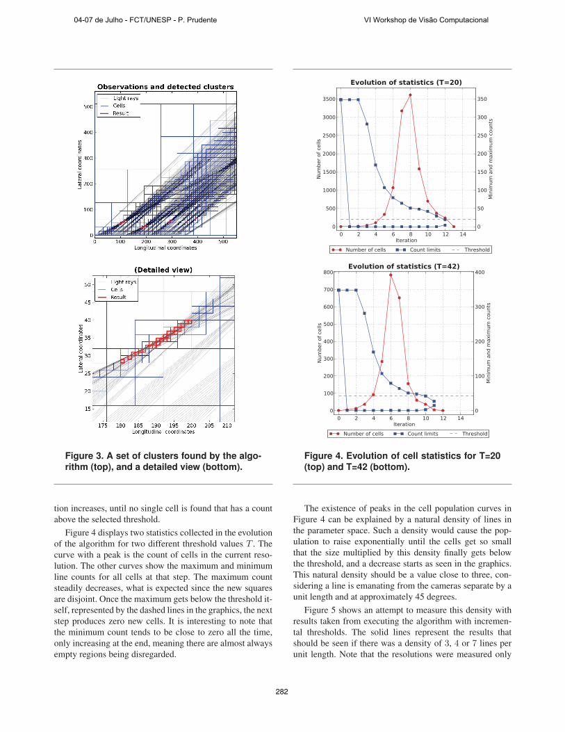
Figure 3. A set of clusters found by the algo-rithm (top), and a detailed view (bottom).

tion increases, until no single cell is found that has a count

above the selected threshold.

Figure 4 displays two statistics collected in the evolution

of the algorithm for two different threshold values T . The

curve with a peak is the count of cells in the current reso-

lution. The other curves show the maximum and minimum

line counts for all cells at that step. The maximum count

steadily decreases, what is expected since the new squares

are disjoint. Once the maximum gets below the threshold it-

self, represented by the dashed lines in the graphics, the next

step produces zero new cells. It is interesting to note that

the minimum count tends to be close to zero all the time,

only increasing at the end, meaning there are almost always

empty regions being disregarded.

0 2 4 6 8 10 12 14

Iteration

0

500

1000

1500

2000

2500

3000

3500

Number of cells

Evolution of statistics (T=20)

0

50

100

150

200

250

300

350

Minimum and maximum counts

Number of cells Count limits Threshold

0 2 4 6 8 10 12 14

Iteration

0

100

200

300

400

500

600

700

800

Number of cells

Evolution of statistics (T=42)

0

100

200

300

400

Minimum and maximum counts

Number of cells Count limits Threshold

Figure 4. Evolution of cell statistics for T=20

(top) and T=42 (bottom).

The existence of peaks in the cell population curves in

Figure 4 can be explained by a natural density of lines in

the parameter space. Such a density would cause the pop-

ulation to raise exponentially until the cells get so small

that the size multiplied by this density finally gets below

the threshold, and a decrease starts as seen in the graphics.

This natural density should be a value close to three, con-

sidering a line is emanating from the cameras separate by a

unit length and at approximately 45 degrees.

Figure 5 shows an attempt to measure this density with

results taken from executing the algorithm with incremen-

tal thresholds. The solid lines represent the results that

should be seen if there was a density of 3, 4 or 7 lines per

unit length. Note that the resolutions were measured only


282

in power-of-two values, causing the staircase shape of the

measurements curve. The linear model does approximate

the results, but a power law seems to approximate better.

The dashed curves in the graphic represent a power law with

1.15 exponent instead of 1 as in the linear model. This phe-

nomenon should be further investigated in the future in or-

der to allow the prediction of the natural density of points

and in consequence the step where a peak in cell popula-

tion will happen, and what should be the number.

10

0

10

1

10

2

10

3

Miminum count

10

0

10

1

10

2

Cell size

Resolution for maximum number of cells

Measurements

Linear model

Power model

Figure 5. Possible power law in equivalent

density estimation. The minimum count is T .

3. Experiments

The algorithm was applied to data taken from a video

recorded with a miniDV camcorder carried through a hall-

way in an office environment, tied to a stabilizing device in

order to reduce hand-shaking effects. The features were ex-

tracted as described in [18]. The camera was assumed to be

moving in uniform motion, with unit length distances be-

tween each frame position, as mentioned previously. Also,

as mentioned, only the furthest detection in image coordi-

nates was considered for each frame, for a single half of the

images. The result of applying the algorithm to this dataset

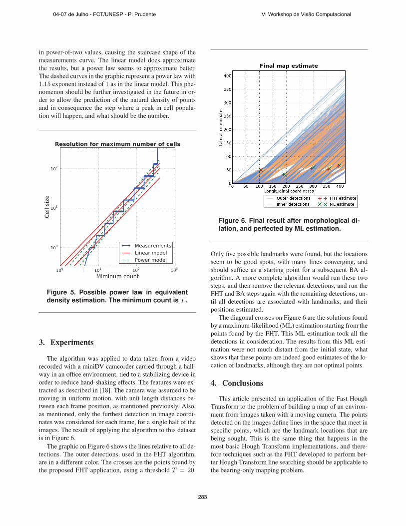
is in Figure 6.

The graphic on Figure 6 shows the lines relative to all de-

tections. The outer detections, used in the FHT algorithm,

are in a different color. The crosses are the points found by

the proposed FHT application, using a threshold T = 20.

Figure 6. Final result after morphological di-lation, and perfected by ML estimation.

Only five possible landmarks were found, but the locations

seem to be good spots, with many lines converging, and

should suffice as a starting point for a subsequent BA al-

gorithm. A more complete algorithm would run these two

steps, and then remove the relevant detections, and run the

FHT and BA steps again with the remaining detections, un-

til all detections are associated with landmarks, and their

positions estimated.

The diagonal crosses on Figure 6 are the solutions found

by a maximum-likelihood (ML) estimation starting from the

points found by the FHT. This ML estimation took all the

detections in consideration. The results from this ML esti-

mation were not much distant from the initial state, what

shows that these points are indeed good estimates of the lo-

cation of landmarks, although they are not optimal points.

4. Conclusions

This article presented an application of the Fast Hough

Transform to the problem of building a map of an environ-

ment from images taken with a moving camera. The points

detected on the images define lines in the space that meet in

specific points, which are the landmark locations that are

being sought. This is the same thing that happens in the

most basic Hough Transform implementations, and there-

fore techniques such as the FHT developed to perform bet-

ter Hough Transform line searching should be applicable to

the bearing-only mapping problem.


283

The use of this technique is a good match to other classic

BA techniques where an initial position of landmarks must

be provided prior to execution. The execution of the FHT

depends only on the definition of a large initial search area,

the threshold and the stop criteria. A complete SLAM sys-

tem could then be devised with a larger loop with two steps:

the execution of the FHT to find new landmark candidates

followed by ML estimation of optimal landmark positions

and camera locations. New iterations will consider disasso-

ciated detections and propose new landmarks, until all de-

tections are solved. While the landmark estimates found in

this experiment were quite good, the ML step is still neces-

sary to find the actual ML optimum estimates, perform more

sophisticated feature matching, and also to solve the com-

plete SLAM problem, since the presented technique per-

forms only mapping.

More research is needed on the determination of the

threshold and the stop criteria to allow autonomous oper-

ation. The investigation of how to adapt the system to real-

time operation is also interesting. Of course, the complete

two-stage BA system proposed must also be evaluated.

Acknowledgements

For their support: National Council for Scentific and

Technological Development (CNPq N. 475690/2008-7),

Foundation for Research Support of Sao Paulo (FAPESP,

N. 2008/03995-5), and National Council for the Improve-

ment of Higher Education (CAPES).

References

[1] R. Barra, C. Ribeiro, and A. H. R. Costa. Fast vertical line

correspondence between images for mobile robot localiza-

tion. In 9th International IFAC Symposium on Robot Control

(SYROCO2009), pages 153–158, 2009.

[2] S. Choi, T. Kim, and W. Yu. Performance evaluation of

ransac family. In 20th British Machine Vision Conference,

2009.

[3] A. Davison, I. Reid, N. Molton, and O. Stasse. MonoSLAM:

Real-time single camera SLAM. Pattern Analysis and Ma-

chine Intelligence, IEEE Transactions on, 29(6):1052 –1067,

june 2007.

[4] H. Durrant-Whyte and T. Bailey. Simultaneous localization

and mapping: part I. Robotics Automation Magazine, IEEE,

13(2):99 –110, june 2006.

[5] E. Eade and T. Drummond. Edge landmarks in monocular

SLAM. Image Vision Comput., 27(5):588–596, 2009.

[6] J. Illingworth and J. Kittler. A survey of the hough trans-

form. Comput. Vision Graph. Image Process., 44(1):87–116,

1988.

[7] Q. Ke and T. Kanade. Quasiconvex optimization for robust

geometric reconstruction. In In International Conference on

Computer Vision, pages 986–993, 2005.

[8] S. Kim and S.-Y. Oh. SLAM in indoor environments using

omni-directional vertical and horizontal line features. J. In-

tell. Robotics Syst., 51(1):31–43, 2008.

[9] H. Li, M. A. Lavin, and R. J. Le Master. Fast hough trans-

form: A hierarchical approach. Computer Vision, Graphics

and Image Processing, 36(2-3):139–161, 1986.

[10] J. Neira, A. J. Davison, and J. J. Leonard. Guest editorial spe-

cial issue on visual SLAM. Robotics, IEEE Transactions on,

24(5):929 –931, oct. 2008.

[11] J. Sola. Consistency of the EKF-SLAM algorithm for three

different landmark parametrizations. In 2010 IEEE Interna-

tional Conference on Robotics and Automation, 2010.

[12] R. Stephens. Probabilistic approach to the hough transform.

Image and Vision Computing, 9(1):66 – 71, 1991. The first

BMVC 1990.

[13] H. Strasdat, J. M. M. Montiel, and A. Davison. Real-time

monocular SLAM: Why filter? In Robotics and Automation,

2010. ICRA ’10. IEEE International Conference on, 2010.

[14] S. Thrun. Robotic mapping: a survey. In Exploring artifi-

cial intelligence in the new millennium, pages 1–35. Morgan

Kaufmann Publishers Inc., San Francisco, CA, USA, 2003.

[15] P. H. S. Torr and A. Zisserman. Mlesac: A new robust esti-

mator with application to estimating image geometry. Com-

puter Vision and Image Understanding, 78:2000, 2000.

[16] B. Triggs, P. F. McLauchlan, R. I. Hartley, and A. W. Fitzgib-

bon. Bundle adjustment - a modern synthesis. In ICCV ’99:

Proceedings of the International Workshop on Vision Algo-

rithms, pages 298–372, London, UK, 2000. Springer-Verlag.

[17] N. L. Werneck and A. H. R. Costa. Mapping with monocular

vision in two dimensions. International Journal of Natural

Computing Research, 1, 2010. In press.

[18] N. L. Werneck, A. H. R. Costa, and F. S. Truzzi. Medicao de

distancia e altura de bordas horizontais com visao monocular

linear para robos moveis. In Anais do V Workshop de Visao

Computacional, 2009.

[19] M. Wongphati, N. Niparnan, and A. Sudsang. Bearing only

FastSLAM using vertical line information from an omnidi-

rectional camera. In ROBIO ’09: Proceedings of the 2008

IEEE International Conference on Robotics and Biomimet-

ics, pages 1188–1193, Washington, DC, USA, 2009. IEEE

Computer Society.


284

monocular visual mapping with the fast hough transformnwerneck.sdf.org/almoxarifado/72827.pdfand is...

Documents