monopoly pricing in vertical markets with demand uncertainty
TRANSCRIPT

Monopoly Pricing in Vertical Markets with Demand Uncertainty
Stefanos Leonardosa,∗, Costis Melolidakisb, Constandina Kokic
aSingapore University of Technology and Design, 8 Somapah Rd, 487372 SingaporebNational and Kapodistrian University of Athens, Panepistimioupolis, 15784 Athens, GreececAthens University of Economics and Business, 76 Patission Street, 10434 Athens, Greece
Abstract
Motivation: Pricing decisions are often made when market information is still poor. Whilemodern pricing analytics aid firms to infer the distribution of the stochastic demand that theyare facing, data-driven price optimization methods are often impractical or incomplete if notcoupled with testable theoretical predictions. In turn, existing theoretical models often reasonabout the response of optimal prices to changing market characteristics without exploiting allavailable information about the demand distribution. Academic/practical relevance: Ouraim is to develop a theory for the optimization and systematic comparison of prices betweendifferent instances of the same market under various forms of knowledge about the correspond-ing demand distributions. Methodology: We revisit the classic problem of monopoly pricingunder demand uncertainty in a vertical market with an upstream supplier and multiple formsof downstream competition between arbitrary symmetric retailers. In all cases, demand uncer-tainty falls to the supplier who acts first and sets a uniform price before the retailers observethe realized demand and place their orders. Results: Our main methodological contributionis that we express the price elasticity of expected demand in terms of the mean residual de-mand (MRD) function of the demand distribution. This leads to a closed form characterizationof the points of unitary elasticity that maximize the supplier’s profits and the derivation ofa mild unimodality condition for the supplier’s objective function that generalizes the widelyused increasing generalized failure rate (IGFR) condition. A direct implication is that optimalprices between different markets can be ordered if the markets can be stochastically ordered ac-cording to their MRD functions or equivalently, their elasticities. Using the above, we developa systematic framework to compare optimal prices between different market instances via therich theory of stochastic orders. This leads to comparative statics that challenge previouslyestablished economic insights about the effects of market size, demand transformations and de-mand variability on monopolistic prices. Managerial implications: Our findings complementdata-driven decisions regarding price optimization and provide a systematic framework usefulfor making theoretical predictions in advance of market movements.
Keywords: Monopoly Pricing, Revenue Maximization, Demand Uncertainty, PricingAnalytics, Comparative Statics, Stochastic Orders, Unimodality2010 MSC: 91A10, 91A65, 91B54
1. Introduction
Making optimal pricing decisions is a crucial driver for firms’ profitability and a well-studiedproblem in the existing theoretical literature. However, modern markets pose novel opportuni-ties and challenges for firms’ pricing decisions. On the one hand, the sheer amount of historical
∗Corresponding authorEmail addresses: [email protected] (Stefanos Leonardos), [email protected] (Costis
Melolidakis), [email protected] (Constandina Koki)
Preprint submitted to Annals of Operations Research July 19, 2021
arX
iv:1
709.
0961
8v7
[m
ath.
OC
] 1
6 Ju
l 202
1

price/demand data and the wide range of pricing analytics methods allow firms to make moreinformed decisions. One the other hand, the inherent volatility of contemporary economiesfrequently renders such data-driven methods impractical. Sellers, often launch new or differ-entiated products for which demand is unknown or introduce existing products to unchartedemerging markets (Cohen et al., 2016). In other cases, firms act as wholesalers in foreign marketsfor which they have asymmetrically less information than local retailers or sell their productsover competitive digital platforms to highly diversified clienteles (Chen et al., 2018). More gen-erally, firms often need to test the outcome of price changes in advance of anticipated marketmovements or to constantly adjust their prices in periods of turbulent market conditions.
Common in all these cases is that firms have to make important pricing decisions whenmarket information is still poor (Li and Atkins, 2005). While uncertainties can be mitigatedvia marketing strategies or contracting schemes between the members of the supply chain, afterall efforts, some uncertainty persists and the final point of interaction between wholesalers andretailers or more generally, between sellers and buyers is the selling price (Li and Petruzzi, 2017;Berbeglia et al., 2019).
Whenever possible, pricing analytics on historic price/demand data aid firms to build upknowledge about the (probability) distribution of the uncertain demand. The main challengelies in leveraging this information to set and adjust prices optimally. However, data-drivenapproaches that extrapolate past trends to make forward-looking pricing decisions may lead tosuboptimal decisions if not coupled with or benchmarked against testable theoretical predic-tions. In turn, existing theoretical tools to optimize and compare prices across different marketinstances (instances of the same market that correspond to different demand distributions) arestill under development (Xu et al., 2010) or make partial use of the available information, e.g.,rely on summary statistics (Lariviere and Porteus, 2001). Moreover, from a managerial perspec-tive, such methods often provide optimality conditions that are not easy to assess in practiceor which do not provide intuitive and economic interpretable results (Van den Berg, 2007).
Model. Motivated by the above, we revisit the classic problem of monopoly pricing with demanduncertainty under the informational assumption that the firm knows the probability distributionof the uncertain demand. This distribution may reflect the seller’s informed belief or estimationsaggregated from historical data. Our purpose is to link the properties of the demand distributionto economic interpretable conditions and to develop a systematic theoretical framework in whichthe firm can optimally set and adjust its prices according to changing market characteristics.
To account for the large variety of market structures that modern sellers are facing, wemodel the monopolistic firm as an upstream supplier who sells its product via a downstreammarket. The downstream market comprises an arbitrary number of retailers and various formsof market competition between the retailers, such as differentiated Cournot and Bertrand com-petition, no or full returns and collusions (cf. Table 1).1 In all cases, retail demand is linear. Inthe first stage, the monopolistic firm sets a uniform price and in the second stage, the retailersobserve the price and place their orders after the market demand has been realized. We as-sume that the supplier’s capacity exceeds potential demand and that downstream retailers aresymmetric. These assumptions serve the purpose to isolate the study of pricing decisions underuncertainty from various other strategic considerations such as stocking decisions, negotiationpower, marketing and production (Xue et al., 2017; Dong et al., 2019).2
1The two-tier market model is an abstraction to capture the complexity of current markets. If we eliminatethe second stage and assume that the supplier sells directly to the consumers, then our results still apply.
2Under these assumptions, i.e., if the supplier’s capacity exceeds potential demand and if the retailers aresymmetric, then the single price scheme is optimal among a wide range of possible pricing mechanisms (Harrisand Raviv, 1981; Riley and Zeckhauser, 1983). In addition, the symmetry of the retailers allows the study ofpurely competitive aspects which is not possible if retailers are heterogeneous Tyagi (1999).
2

Results. Our main theoretical contribution is that we characterize the seller’s optimal pricesas fixed points of the mean residual demand (MRD) function of the stochastic demand level.Informally, if α, r denote the random demand level and the supplier’s price respectively, thenany optimal price, r∗, satisfies the equation r∗ = m (r∗), where m (r) := E (α− br | α > br) andb is a proper scaling constant (that can be normalized to b = 1). The MRD function measuresthe expected additional demand given that demand has reached or exceeded a threshold br.3
This characterization stems from the observation that the price elasticity of expected demandcan be expressed in terms of the MRD function as r/m (r), cf. equation (8). Thus, optimalprices that correspond to points of unitary elasticity are fixed points of the MRD function. Ifm (r) /r is decreasing (or equivalently, if the price elasticity is increasing), then there exists aunique such optimal price. Both statements are presented in Theorem 3.2.
The above unimodality condition for the otherwise not necessarily concave nor quasi-concaveseller’s revenue function, strictly generalizes the well-known increasing generalized failure rate(IGFR) condition (Lariviere and Porteus, 2001; Van den Berg, 2007). Given the inclusivenessof the IGFR conditions, this suggests that Theorem 3.2 applies to essentially most distribu-tions that are commonly used in economic modeling (Paul, 2005; Lariviere, 2006; Banciu andMirchandani, 2013). The expressions of the price elasticity of expected demand and the seller’soptimal price in terms of well-understood characteristics of the demand distribution (MRDfunctions) offer a novel perspective to the otherwise standard linear stochastic model.4 Theyprovide conditions that are easy to assess in practice and which can be useful to gain intuitiveand economic interpretable results (Van den Berg, 2007). In particular, these expressions pro-vide a novel way to derive comparative statics on the response of the optimal price to variousmarket characteristics (expressed as properties of the demand distribution) and to measuremarket performance.
The key intuition along this line, which is formally established in Lemma 4.2, is that theseller’s optimal price is higher in less elastic markets which are precisely markets that canbe ordered in the MRD stochastic order. In other words, if two demand distributions can beordered in terms of their MRD functions, then the supplier’s optimal price is higher in themarket with the dominating MRD function. Thus, the fact that elasticity is a critical factor insetting profitable prices and an important determinant of price changes in response to demandchanges is formalized in terms of well-known demand characteristics. As a result, Lemma 4.2 isthe key to leverage the theory of stochastic orders as a tool to compare prices in markets withdifferent characteristics, such as market size and demand variability. Stochastic orders takeinto account various characteristics of the underlying demand distribution going thus, beyondsummary statistics such as expectation or standard deviation, which provide a limited amountof information (Shaked and Shanthikumar, 2007).
In the comparative statics analysis, we start with the effect of market size in optimal pricesand ask whether larger markets give rise to higher prices. Our first finding is that stochasticallylarger markets do not necessarily lead to higher wholesale prices (Section 4.2.1). Technically,this follows from the fact that the usual stochastic order does not imply (nor is implied by) the�mrd-order (Shaked and Shanthikumar, 2007). Hence, the intuition of Lariviere and Porteus(2001) that “size is not everything” and that prices are driven by different forces is justified
3In reliability applications, this function is known as the mean residual life (MRL), see Shaked and Shanthiku-mar (2007); Lai and Xie (2006); Belzunce et al. (2013, 2016).
4While our results directly apply to the more general demand function of Lopez and Vives (2019), we stick tothe linear model for expositional purposes. Except from the fact that linear markets have been consistently inthe spotlight of economic research both due to their tractability and their accurate modeling of real situations,the study of the linear model is also technically motivated by Cohen et al. (2016) who demonstrate that wheninformation about demand is limited, firms may act efficiently as if demand is linear. For practical purposes,this yields a simple and low regret pricing rule and provides a motivation to study linear markets in a systematicway.
3

by an appropriate theoretical framework. As Lemma 4.2 demonstrates, the correct criterion toorder prices is the elasticity of different market instances rather than their size. In Theorem 4.3,we use this to derive a collection of demand transformations that preserve the MRD order (i.e.,the elasticity) and hence the order of optimal prices. Returning to the effects of market size,one may still ask whether there exist conditions under which a probabilistic increase in marketdemand will lead to an increase in optimal prices. This question is addressed in Theorem 4.5,where we show that this is indeed the case whenever the initial demand is increased by a scalefactor greater than one or (under some mild additional conditions) whenever an additionaldemand source is aggregated.
Next, we turn to the effect of demand variability. Does the seller charge higher/lower pricesin more variable markets? The answer to this question again depends on the exact notionof variability that will be used. Under mild additional assumptions, Theorem 4.6 gives twovariability orders that preserve monotonicity: in both cases the seller charges a lower price inthe less variable market. This conclusion remains true under the mean preserving transformationthat is used by Li and Atkins (2005); Li and Petruzzi (2017). However, as was the case withmarket size, the general statement that more variable markets give rise to higher prices doesnot hold. In Section 4.3.3, we provide an example to show that this generalization fails inthe standard case of parametric families of distributions that are compared in terms of theircoefficient of variation, cf. Lariviere and Porteus (2001). All results from the comparativestatics analysis are summarized in Table 2.
We then turn to measure market performance and efficiency. Our main result in this di-rection, is a distribution-free (over the class of distributions with decreasing MRD function)upper bound on the probability of a stockout, i.e., of no trade between the supplier and theretailers (Theorem 5.1). As shown in Examples 5.2, 5.3 and 5.4, this bound is tight and cannotbe further generalized to distributions with increasing price elasticity of expected demand. Incase that trade takes place, we measure market efficiency in terms of the realized profits andtheir distribution between the supplier and the retailers. Our results are summarized in The-orem 5.5. As intuitively expected (and in line with earlier results, cf. Ai et al. (2012)), thesupplier’s profits are always higher if he is informed about the exact demand level and whenretail competition is higher. However, there exists a range of intermediate demand realizationsfor which the supplier captures a larger share of the aggregate profits in the stochastic market.
Finally, we compare the aggregate realized profits between the deterministic and stochasticmarkets. The outcomes depend on the interplay between demand uncertainty and the level ofretail competition. More specifically, there exists an interval of demand realizations for whichthe aggregate profits of the stochastic market are higher than the profits of the deterministicmarket. The interval reduces to a single point as the number of downstream retailers increases,but is unbounded in the case of 2 retailers. In particular, for n = 1, 2, the aggregate profitsof the stochastic market remain strictly higher than the profits of the deterministic market forall large enough realized demand levels. However, the performance of the stochastic market incomparison to the deterministic market degrades linearly in the number of competing retailersfor demand realizations beyond this interval. This shows that uncertainty on the side of thesupplier is more detrimental for the aggregate market profits when the level of retail competitionis high, cf. Theorem 5.6.
1.1. Related Literature
The study of price-only contracts under demand uncertainty has been long motivated byHarris and Raviv (1981); Riley and Zeckhauser (1983) who show that committing to a singleprice is the optimal pricing strategy if the supplier’s capacity exceeds potential demand andretailers are symmetric or if the monopolist is facing a known demand distribution. If themonopolist does not know the distribution of demand a-priori, as we assume in the presentpaper, then dispersed pricing improves upon the performance of a uniform price Dana (2001).
4
By contrast, Ai et al. (2012) show that wholesale price contracts are optimal even in the caseof two competing chains. Compelling arguments for the linear pricing scheme are also providedin Tyagi (1999); Hwang et al. (2018) and references within. Perakis and Roels (2007) andBernstein and Federgruen (2005) argue that apart from their practical prevalence, price-onlycontracts are relevant in modeling worst-case scenarios or interaction between sellers and buyersin cases with remaining uncertainty, i.e., after any efforts have been made to reduce the initialuncertainty through more elaborate schemes. This is further supported by Li and Petruzzi(2017) who find that in a vertical market with a single manufacturer and a single retailer thatis governed by a wholesale contract between them, less uncertainty may harm either or bothmembers of the supply chain. This is partially the case also in the current model as we showin Section 5.2.1. In particular, we find demand realizations for which the stochastic marketoutperforms the deterministic market in terms of aggregate profits. However, in our model, thesupplier is always better off with reduced uncertainty whereas the retailers may be not.
The vertical market of a single supplier and multiple downstream competing retailers hasbeen widely studied from different perspectives (Padmanabhan and Png, 1997; Tyagi, 1999;Yang and Zhou, 2006; Wu et al., 2012). Our results in Theorems 5.5 and 5.6 are comparablewith or mirror earlier findings in this line of literature. However, in the current setting, thesefindings complement our main results on the characterization of the demand elasticity in terms ofthe MRD function and the resulting comparative statics rather than being the main focus of ourstudy. Concerning its other assumptions (market structure and timing of demand realization),our model enjoys similarities with the model of De Wolf and Smeers (1997). For extensivesurveys of similar demand models, we refer to Huang et al. (2013) and for earlier studies to Yaoet al. (2006). Indicatively, the additive demand model with linear deterministic component isused by Petruzzi and Dada (1999) and Ye and Sun (2016).
Regarding the derived unimodality conditions, our findings are most closely related to Lar-iviere (2006); Van den Berg (2007) who derive the IGFR unimodality condition in the settingof one seller and one buyer. These are special cases of the present setting and, accordingly, theIGFR condition is a restriction of the unimodality condition in terms of the MRD function thatwe formulate in the current setting. IGFR distributions were first used in economic applica-tions by Singh and Maddala (1976) and were popularized in the context of revenue managementby Lariviere and Porteus (2001). Technical aspects of IGFR distributions are studied in Paul(2005); Banciu and Mirchandani (2013). These results are more closely related to a companionpaper (Leonardos and Melolidakis, 2020), in which the authors focus on the technical propertiesof distributions that satisfy the current unimodality condition in terms of the MRD function.5
The MRD function also arises naturally in many revenue management problems with demanduncertainty, see e.g., Mandal et al. (2018); Luo et al. (2016); Colombo and Labrecciosa (2012);Song et al. (2009, 2008) and Petruzzi and Dada (1999) for a non-exhaustive list of related pa-pers. However, to the best of our knowledge, there is no formal link between the elasticity ofuncertain demand and the MRD function or the theory of stochastic orders in these papers.
Similarities regarding the technical analysis can also be found between the current modeland the literature on the price-setting newsvendor under stochastic demand, see e.g., Chenet al. (2004); Kyparisis and Koulamas (2018); Rubio-Herrero and Baykal-Gursoy (2018); Ko-cabıyıkoglu and Popescu (2011); Kouvelis et al. (2018). However, as the rest of the literatureabout the newsvendor, these results involve inventory considerations and hence are quite distinctfrom ours.
More closely related to the current methodology is the study of Xu et al. (2010). This paperis quite distinct from ours since it focus on a restricted set of stochastic orders and in a differentnewsvendor model that involves both pricing and stocking decisions. Concerning the results,
5Other closely related papers in the same direction include Leonardos and Melolidakis (2020a,b, 2021), pre-liminary versions of which appear in Melolidakis et al. (2018); Koki et al. (2018).
5

Xu et al. (2010) show that a stochastically larger demand leads to higher selling prices for theadditive demand case. We extend these findings by showing that different notions of marketsize still lead to the same conclusion under certain conditions (Theorems 4.3 and 4.5) and byproviding a case under which prices may be actually lower in a stochastically larger market,cf. Section 4.2.1. Within similar contexts, Lariviere and Porteus (2001); Li and Atkins (2005);Krishnan (2010); Chen et al. (2017) show that in general, optimal prices decrease as variabilityincreases. Our current set of results refines these findings by using a wide range of stochasticorders that capture different notions of demand variability. Our findings suggest that increaseddemand variability may lead to both increased or decreased prices depending on the notion ofvariability that will be employed (cf. Section 4.3). This demonstrates how various forms ofknowledge about the demand distribution can be useful in the study of price movements andprovides a theoretical explanation for empirically observed price changes in periods of turbulentmarket conditions.
1.2. Outline
The rest of the paper is structured as follows. In Sections 2 and 3, we define and analyzeour model. Section 4 contains the comparative statics and Section 5 the study of marketperformance. Section 6 concludes the paper.
2. The Model
We consider a vertical market with a monopolistic upstream supplier or seller, selling ahomogeneous product (or resource) to n = 2 downstream symmetric retailers who compete ina market with retail demand level α6. The supplier produces at a constant marginal cost whichwe normalize to zero. This corresponds to the situation in which the supplier’s capacity exceedspotential demand by the retailers and the supplier’s lone decision variable is his wholesale price,or equivalently his profit margin, r ≥ 0.
The supplier acts first (Stackelberg leader) and applies a linear pricing scheme withoutprice differentiation, i.e., he chooses a unique wholesale price, r ≥ 0, for all retailers. Weconsider a market setting in which the supplier is less informed than the retailers about theretail demand level α. 7 To model this, we assume that after the supplier’s pricing decision butprior to the retailers’ order decisions, a value for α is realized from a continuous (not-atomic)cumulative distribution function (cdf) F , with finite mean Eα < ∞ and nonnegative values,i.e., F (0) = 0. Equivalently, F can be thought of as the supplier’s belief about the demandlevel and, hence, about the retailers’ willingness-to-pay his price. We write F := 1 − F forthe tail distribution of F and f for its probability density function (pdf) whenever it exists.The support of F is denoted by S, with lower bound L = sup {r ≥ 0 : F (r) = 0} and upperbound H = inf {r ≥ 0 : F (r) = 1} such that 0 ≤ L ≤ H ≤ ∞. We don’t make any additionalassumption about S: in particular, it may or may not be an interval. The case L = H is notexcluded8 and corresponds to the situation in which the supplier is completely informed aboutthe retail demand level.
Given the demand realization α, the aggregate quantity q (r | α) :=∑2
i=1 qi (r | α) that theretailers will order from the supplier is a function of the posted wholesale price r. Assuming
6To ease the exposition, we restrict to n = 2 retailers. As we show in Section 3.3, our results admit astraightforward generalization to arbitrary number n of symmetric retailers.
7We will refer to α throughout as the demand level. However, based on equation (2), α is also known as thechoke or reservation price. Since, these constants are equivalent up to some transformation in our model, thisshould cause no confusion.
8Formally, this case contradicts the assumption that F is continuous or non-atomic. It is only allowed to avoidunnecessary notation and should cause no confusion.
6

risk neutrality, the supplier aims to maximize his expected profit function Πs, which is equal to
Πs (r) = r · Eαq (r | α) . (1)
The quantity q (r | α) depends on the form of second stage competition between the retailers.In this paper, we focus on markets with linear demand as in Mills (1959); Petruzzi and Dada(1999); Huang et al. (2013) and Cohen et al. (2016) among others, and allow for a wide rangeof competition structures between the retailers (Table 1). All these structures give rise – inequilibrium – to the same (up to a scaling constant) functional form for q (r | α) and henceto the same mathematical expression for the supplier’s objective function. More importantly,in all these structures, the second-stage equilibrium between the retailers is unique and hence,q (r | α) is uniquely determined under the assumption that the retailers follow their equilibriumstrategies in the game induced by each wholesale price r ≥ 0 (subgame perfect equilibrium).Specifically, we assume that each retailer i faces the inverse demand function
pi = α− βqi − γqj , (2)
for j = 3− i and i = 1, 2. Here, α/ (β + γ) denotes the potential market size (primary demand),β/(β2 − γ2
)> 0 the store-level factor and γ/β the degree of product differentiation or substi-
tutability between the retailers (Singh and Vives, 1984; Wu et al., 2012). As usual, we assumethat β ≤ γ. Each retailer’s only cost is the wholesale price r ≥ 0 that she pays to the supplier.Hence, each retailer aims to maximize her profit function Πi, which is equal to
Πi (qi, qj) = qi (pi − r) . (3)
Given the demand realization α, the equilibrium quantities q∗i := q∗i (r | α) that maximize Πi fori = 1, 2 are given for various retail market structures in Table 1 as functions of the wholesale pricer. Here, (α− r)+ denotes the positive part, i.e., (α− r)+ := max {0, α− r}. The assumptionof no uncertainty on the side of retailers about the demand level α implies that q∗i correspondsboth to the quantity that each retailer orders from the supplier and to the quantity that shesells to the market.
The standard Cournot and Betrand outcomes arise as special cases of the above. In par-ticular, for γ = 0, the goods are independent and the monopoly solution q∗i = 1
2β (α− r)+ for
i = 1, 2 prevails. For γ = β > 0, the goods are perfect substitutes with q∗i = 12β (α− r)+ in
Bertrand competition (at zero price) and q∗i = 13β (α− r)+ in Cournot competition for i = 1, 2.
All of the above are assumed to be common knowledge among the participants in the market(the supplier and the retailers).
3. Equilibrium analysis: supplier’s optimal wholesale price
We restrict attention to subgame perfect equlibria of the extensive form, two-stage game.9
Assuming that at the second stage, the retailers play their unique equilibrium strategies (q∗1, q∗2),
then, according to (1), the supplier will maximize Π∗s (r) = r ·Eαq∗ (r | α). For the competitionstructures of Table 1, q∗ (r | α) has the general form q∗ (r | α) = λM (α− r)+, where λM >0 is a suitable model-specific constant. Thus, at equilibrium, the supplier’s expected profitmaximization problem becomes
maxr≥0
Π∗s (r) = λM ·maxr≥0
rE (α− r)+. (4)
From the supplier’s perspective, we are interested in finding conditions such that the maximiza-tion problem in (4) admits a unique and finite optimal wholesale price, r∗ ≥ 0.
9Technically, these are perfect Bayes-Nash equilibria, since the supplier has a belief about the retailers’ types,i.e., their willingness-to-pay his price, that depends on the value of the stochastic demand parameter α.
7

Retail market structure Retailer i’s equilibrium order
Singh and Vives (1984)
Cournot competition – product differentiation q∗i = 12β+γ (α− r)+
Bertrand competition – product differentiation q∗i = β(2β−γ)(β+γ) (α− r)+
Padmanabhan and Png (1997)
Single retailer no/full returns q∗ = 12β (α− r)+
Competing retailers (orders/price) – no returns q∗i = 12β+γ (α− r)+
Competing retailers (orders/price) – full returns q∗i = β(2β−γ)(β+γ) (α− r)+
Yang and Zhou (2006)
Collusion between retailers – product differentiation q∗i = 1β+γ (α− r)+
Table 1. Second-stage market structures (first column) and quantities, q∗i , of retailer i ordered from the supplierin equilibrium (second column). The equilibrium quantities are equal – up to a multiplicative constant – andunique which implies that the supplier’s maximization problem is essentially the same for any of these forms ofdownstream competition.
Remark 3.1. The vertical market structure is not necessary for our analysis to hold. In fact, ifwe eliminate the downstream market and instead assume that the firm sells directly to a marketwith inverse linear demand function q (r) = α− βr, then our analysis still applies. This followsfrom the observation that in this case, the seller’s expected profit maximization problem is
maxr≥0
Πs (r) = maxr≥0
rE (α− βr)+
which is the same as the maximization problem in equation (4) after normalizing β to 1.
3.1. Deterministic Market
First, we treat the case in which the supplier knows the primary demand α (deterministicmarket). According to the notation introduced in Section 2, this corresponds to the case α =L = H. In this case Π∗s (r) = λMr (α− r)+ and it is straightforward that r∗ (α) = α/2. Hence,the complete information two-stage game has a unique subgame perfect Nash equilibrium, underwhich the supplier sells with optimal price r∗ (α) = α/2 and each retailer orders quantity q∗i asdetermined by Table 1.
3.2. Stochastic Market
The equilibrium behavior of the market in which the supplier does not know the demand level(stochastic market) is less straightforward. Now, L < H and the supplier is interested in findingan r∗ that maximizes his expected profit in (4). For an arbitrary demand distribution F , Π∗s (r)may not be concave (nor quasi-concave) and, hence, not unimodal, in which case the solutionto the supplier’s optimization problem is not immediate. To obtain a general unimodalitycondition, we proceed by differentiating the supplier’s revenue function Π∗s (r). First, since(α− r)+ is nonnegative, we write E (α− r)+ =
∫∞0 P
((α− r)+ > u
)du =
∫∞r F (u) du, for
0 ≤ r < H. Since Eα <∞ and F is non-atomic by assumption, we have that
d
drE (α− r)+ =
d
dr
(Eα−
∫ r
0F (u) du
)= −F (r)
8

for any 0 < r < H. With this formulation, both the supplier’s revenue function and itsfirst derivative can be expressed in terms of the mean residual demand (MRD) function ofα. In general, the MRD function, m (·), of a nonnegative random variable α with cumulativedistribution function (cdf) F and finite expectation, Eα <∞, is defined as
m (r) := E (α− r | α > r) =1
F (r)
∫ ∞r
F (u) du, for r < H (5)
and m (r) := 0, otherwise, see, e.g., Shaked and Shanthikumar (2007); Lai and Xie (2006) orBelzunce et al. (2016)10. Using this notation, we obtain that Π∗s (r) = λMrm (r) F (r) and
dΠ∗sdr
(r) = λM (m (r)− r) F (r) = λMr
(m (r)
r− 1
)F (r) (6)
for 0 < r < H. Based on (6), the first order condition (FOC) for the supplier’s revenue functionis that m (r) = r or equivalently that m (r) /r = 1. We call the expression
` (r) :=m (r)
r, 0 < r < H (7)
the generalized mean residual demand (GMRD) function, see Leonardos and Melolidakis (2020),due to its connection to the generalized failure rate (GFR) function g (r) := rf (r) /F (r),defined and studied by Lariviere (1999) and Lariviere and Porteus (2001). Its meaning isstraightforward: while the MRD function m (r) at point r > 0 measures the expected additionaldemand, given the current demand r, the GMRD function measures the expected additionaldemand as a percentage of the given current demand. Similarly to the GFR function, the GMRDfunction has an appealing interpretation from an economic perspective, since it is related to theprice elasticity of expected or mean demand (PEED), ε (r) = −r · d
drEq (r | α) /Eq (r | α) (Xuet al., 2010). Specifically,
` (r) =m (r)
r=
(− −F (r)
m (r) F (r)· r
)−1
=
(−r ·
ddrE (α− r)+
E (α− r)+
)−1
= ε−1 (r) (8)
which implies that ` (r) corresponds to the inverse of the price elasticity of expected demand(PEED). Hence, in the current setting, demand distributions with decreasing GMRD, (DGMRDproperty), are precisely distributions that describe markets with increasing PEED, (IPEEDproperty). This observation ties the economic property of IPEED to the distributional propertyof DGMRD. Accordingly, we will use the terms DGMRD and IPEED interchangeably.
Using (8), the FOC in (6) asserts that the supplier’s payoff is maximized at the point(s) ofunitary elasticity. For an economically meaningful analysis, since realistic problems must havea PEED that eventually becomes greater than 1 (Lariviere, 2006), we give particular attentionto distributions for which ` (r) eventually becomes less than 1, i.e., distributions for whichr := sup {r ≥ 0 : m (r) ≥ r} is finite. Observe that for a nonnegative random demand α withcontinuous distribution F and finite expectation Eα, m (0) = Eα > 0 and hence r > 0.
Based on these considerations, it remains to derive conditions that guarantee the existenceand uniqueness of an r∗ that satisfies the FOC and to show that this r∗ indeed corresponds to amaximum of the supplier’s revenue function as given in (4). This is established in Theorem 3.2which is the main result of the present Section.
Theorem 3.2 (Equilibrium wholesale prices in the stochastic market). Consider the supplier’smaximization problem maxr≥0 Π∗s (r) = λM ·maxr≥0 rE (α− r)+ and assume that the nonneg-ative demand parameter, α, follows a continuous (non-atomic) distribution F with support Swithin L and H. Then
10In this literature, the MRD function is known as the mean residual life function due to its origins in reliabilityapplications.
9

(a) Necessary condition: If an optimal price r∗ for the supplier exists, then r∗ satisfies the fixedpoint equation
r∗ = m (r∗) . (9)
(b) Sufficient conditions: If the generalized mean residual demand (GMRD) function, ` (r) :=m (r) /r, of F is strictly decreasing and Eα2 is finite, then at equilibrium, the supplier’s optimalprice r∗ exists and is the unique solution of (9). In this case, r∗ = Eα/2, if Eα/2 < L, andr∗ ∈ [L,H), otherwise.
Proof. (a) Since F (r) > 0 for 0 < α < H, the sign of the derivative dΠ∗s
dr (r) is determined bythe term m (r) − r and any critical point r∗ satisfies m (r∗) = r∗. Hence, the necessary part
of the theorem is obvious from (6) and the continuity of dΠ∗s
dr (r). (b) For the sufficiency part,it remains to check that such a critical point exists and corresponds to a maximum under theassumptions that ` (r) is strictly decreasing and Eα2 < ∞. Clearly, m (r) − r is continuousand limr→0+ m (r) − r = Eα > 0. Hence, Π∗s (r) starts increasing on (0, H). However, the
limiting behavior of m (r)− r and hence of dΠ∗s
dr (r) as r approaches H from the left, may varydepending on whether H is finite or not. If H is finite, i.e., if the support of α is bounded, thenlimr→H− (m (r)− r) = −H. Hence, ` (r) eventually becomes less than 1 and a critical point r∗
that corresponds to a maximum exists without any further assumptions. Strict monotonicityof ` (r) implies that this r∗ is unique. If H = ∞, then an optimal solution r∗ may not existbecause the limiting behavior of m (r) as r → ∞ may vary, see Example 3.4 or Bradley andGupta (2003). In this case, the condition of finite second moment ensures that r < ∞. Inparticular, as shown in Leonardos and Melolidakis (2020), if the GMRD function ` (r) of arandom variable α with unbounded support is decreasing, then limr→∞ ` (r) < 1 if and only ifEα2 is finite. This establishes existence. Uniqueness follows again from strict monotonicity of` (r) which precludes intervals of the form m (r) = r that give rise to multiple optimal solutions.
To prove the second claim of the sufficiency part, note that Eα < 2L is equivalent tom (L) < L. Then, the DGMRD property implies that m (r) < r for all r > L, hence r∗ < L.In this case, m (r∗) = Eα − r∗ and hence r∗ is given explicitly by r∗ = Eα/2, which may becompared with the optimal r∗ of the complete information case. On the other hand, if Eα ≥ 2L,then for all r < L, m (r) = Eα− r ≥ 2L− r > r which implies that r∗ must be in [L,H).
The economic interpretation of the sufficiency conditions in part (b) of Theorem 3.2 isimmediate. By (8), demand distributions with the DGMRD property are precisely distributionsthat exhibit increasing PEED (IPEED property). In turn, finiteness of the second moment isrequired to ensure that the expected demand will eventually become elastic, even in the caseof unbounded support, see Leonardos and Melolidakis (2020), Theorem 3.2. Thus, part (b)characterizes in terms of their mathematical properties demand distributions that model linearmarkets with monotone and eventually elastic expected demand. These conditions apply todistributions that may neither be absolutely continuous (do not possess a density) nor have aconnected support.
Remark 3.3. In the statement of Theorem 3.2, strict monotonocity can be relaxed to weakmonotonicity without significant loss of generality. This relies on the explicit characterizationof distributions with MRD functions that contain linear segments which is given in Proposition10 of Hall and Wellner (1981). Namely, m (r) = r on some interval J = [a, b] ⊆ S if and onlyif F (r) r2 = F (a) a2 for all r ∈ J . If J is unbounded, this implies that α has the Paretodistribution on J with scale parameter 2. In this case, Eα2 = ∞, see Example 3.4, which isprecluded by the requirement that Eα2 <∞. Hence, to replace strict by weak monotonicity –but still retain equilibrium uniqueness – it suffices to exclude distributions that contain intervalsJ = [a, b] ⊆ S with b <∞ in their support, for which F (r) r2 = F (a) a2 for all r ∈ J .
10

Example 3.4 (Pareto distribution). The Pareto distribution is the unique distribution withconstant GMRD and GFR functions over its support. Let α be Pareto distributed with pdff (r) = kLkr−(k+1)1{L≤r}, and parameters 0 < L and k > 1 (for 0 < k ≤ 1 we get Eα = ∞,which contradicts the basic assumptions of our model). To simplify, let L = 1, so that f (r) =kr−k−11{1≤r<∞}, F (r) =
(1− r−k
)1{1≤r<∞}, and Eα = k
k−1 . The mean residual demand
of α is given by m (r) = rk−1 + k
k−1 (1− r) 1{0≤r<1} and, hence, is decreasing on [0, 1) andincreasing on [1,∞). However, the GMRD function ` (r) = m (r) /r is decreasing for 0 < r < 1and is constant thereafter, hence, α is DGMRD. Similarly, for 1 ≤ r the failure (hazard) rateh (r) = kr−1 is decreasing, but the generalized failure rate g (r) = k is constant and, hence, αis IGFR. The payoff function of the supplier is
Π∗s (r) = λMrm (r) F (r) =λM
(k − 1)
{r (r − rk + k) if 0 ≤ r < 1
r2−k if r ≥ 1,
which diverges as r → ∞, for k < 2 and remains constant for k = 2. In particular, for k ≤ 2,the second moment of α is infinite, i.e., Eα2 =∞, which shows that for DGMRD distributions,the assumption that the second moment of F is finite may not be dropped for part (b) ofTheorem 3.2 to hold. On the other hand, for k > 2, we get r∗ = k
2(k−1) as the unique optimal
wholesale price, which is indeed the unique fixed point of m (r).
3.3. General case with n identical retailers
To ease the exposition, we restricted our presentation to n = 2 identical retailers. However,the present analysis applies to arbitrary number n ≥ 1 of symmetric retailers for all competition-structures that give rise to a unique second-stage equilibrium in which the aggregate orderedquantity depend on α via the term (α− r)+ as in Table 1. This relies on the fact, that in suchmarkets, the total quantity that is ordered from the supplier depends on n only up to a scalingconstant. Thus, the approach to the supplier’s expected profit maximization in the first-stageremains the same independently of the number of second-stage retailers. To avoid unnecessarynotation, we present the general case for the classic Cournot competition.
Formally, let N = {1, 2, . . . , n}, with n ≥ 1 denote the set of symmetric retailers. A strategyprofile (retailers’ orders from the supplier) is denoted by q = (q1, q2, . . . , qn) with q =
∑nj=1 qj
and q−i := q − qi. Assuming linear inverse demand function p = α − βq, the payoff functionof retailer i, for i ∈ N , is given by Πi (q, q−i) = qi (p− r). Under these assumptions, thesecond stage corresponds to a linear Cournot oligopoly with constant marginal cost, r. Hence,each retailer’s equilibrium strategy, q∗i (r), is given by q∗i (r) = 1
β(n+1) (α− r)+, for r ≥ 0.Accordingly, in the first stage, the supplier’s expected revenue function on the equilibrium pathis given by Π∗s (r) = rq∗ (r) = n
β(n+1)rE (α− r)+. Hence, it is maximized again at r∗ (α) = α/2
if the supplier knows α or at r∗ = m (r∗) if the supplier only knows the distribution F of α.Based on the above, the number of second-stage retailers affects the supplier’s revenue functiononly up to a scaling constant and Theorem 3.2 is stated unaltered for any n ≥ 1.
4. Comparative Statics
The main implication of the closed form expression of the supplier’s optimal price in termsof the MRD function (equation (9)) is that it facilitates a comparative statics analysis via therich theory of stochastic orders (Shaked and Shanthikumar, 2007; Lai and Xie, 2006; Belzunceet al., 2016). Since the equilibrium quantity and price q∗, p∗ are both monotone in the wholesaleprice r∗, our focus will be on r∗ as the demand distribution characteristics vary. To obtain ameaningful comparison between different market instances (i.e., instances of the same market
11

that correspond to different demand distributions), we assume throughout equilibrium unique-ness and hence, unless stated otherwise, we consider only distributions for which Theorem 3.2applies11. First, we introduce some additional notation.
Let X1 ∼ F1, X2 ∼ F2 be two nonnegative random variables – or equivalently demanddistributions – with supports between L1 and H1 and L2 and H2, respectively (cf. definitionof L and H in Section 2) and MRD functions m1 (r) and m2 (r). We say that X1 is less thanX2 in the mean residual demand order, denoted by X1 �mrd X2
12, if m1 (r) ≤ m2 (r) for allr ≥ 0. This order plays a key role in the present model. Specifically, by (8), we have thatm1 (r) ≤ m2 (r) for any r ≥ 0 if and only if ε2 (r) ≤ ε1 (r) for any r ≥ 0, i.e., if and only if theprice elasticity of expected demand in market X2 is less than the price elasticity of expecteddemand in market X1 for any wholesale price r ≥ 0. This motivates the following definition.
Definition 4.1. We will say that market X2 is less elastic than market X1, denoted by X2 �el
X1, if ε2 (r) ≤ ε1 (r) for every r ≥ 0. Based on the above, X2 �el X1 if and only if X1 �mrd X2.
Using this notation, the following Lemma captures the importance of the characterizationof the optimal price via the fixed point equation (9).
Lemma 4.2. Let X1 ∼ F1, X2 ∼ F2 be two nonnegative, continuous and strictly DGMRD de-mand distributions with finite second moments. If X2 is less elastic than X1, then the supplier’soptimal wholesale price is lower in market X1 than in market X2. In short, if X2 �el X1, thenr∗1 ≤ r∗2.
Proof. By definition, X2 �el X1 implies that ε2 (r) ≤ ε1 (r) for every r ≥ 0 which by (8) isequivalent to `1 (r) ≤ `2 (r) for all r ≥ 0. Hence, by (9), 1 = `1 (r∗1) ≤ `2 (r∗1) < `2 (r) for allr < r∗1, where the second inequality follows from the assumption that X2 is strictly DGMRD.Since `2 (r∗2) = 1, it follows that r∗1 ≤ r∗2.
Lemma 4.2 states that the supplier charges a higher price in a less elastic market. Althoughtrivial to prove once Theorem 3.2 has been established, it is the key to the comparative staticsanalysis in the present model. Indeed, combining the above, the task of comparing the optimalwholesale price r∗ for varying demand distribution parameters – such as market size or demandvariability – essentially reduces to comparing demand distributions (market instances) in termsof their elasticities or equivalently in terms of their MRD functions. Such conditions can befound in Shaked and Shanthikumar (2007) and Belzunce et al. (2013) and provide the frameworkfor the subsequent analysis.
4.1. Transformations that preserve the MRD-order
Lemma 4.2 provides a natural starting point to study the response of the equilibrium whole-sale price, r∗, to changes in the demand distribution. In particular, if a change in the demanddistribution preserves the �mrd-order, then Lemma 4.2 readily implies that this change will alsopreserve the order of wholesale prices. Specifically, let X1 ∼ F1, X2 ∼ F2 denote two differentdemand distributions, such that X1 �mrd X2. In this case, we know by Lemma 4.2 that r∗1 ≤ r∗2.We are interested in determining transformations of X1, X2 that preserve the �mrd-order andhence the ordering r∗1 ≤ r∗2. Unless otherwise stated, we assume that the random demand issuch that it satisfies the sufficiency conditions of Theorem 3.2 and hence that the supplier’soptimal wholesale price exists and is unique.
11Since the DGMRD property is satisfied by a very broad class of distributions, see Banciu and Mirchandani(2013), Kocabıyıkoglu and Popescu (2011) and Leonardos and Melolidakis (2020), we do not consider this as asignificant restriction. Still, since it is sufficient (together with finitenes of the second moment) but not necessaryfor the existence of a unique optimal price, the analysis naturally applies to any other distribution that guaranteesequilibrium existence and uniqueness.
12In reliability applications, the MRD-order is commonly known as the mean residual life (MRL)-order, Shakedand Shanthikumar (2007).
12
Theorem 4.3. Let X1 ∼ F1, X2 ∼ F2 denote two nonnegative, continuous and strictly DGMRDdemand distributions, with finite second moments, such that X1 �mrd X2.
(i) If Z is a nonnegative, IFR distribution, independent of X1 and X2, then r∗X1+Z ≤ r∗X2+Z.
(ii) If φ is an increasing, convex function, then r∗φ(X1) ≤ r∗φ(X2).
(iii) If Xp ∼ pF1 + (1− p)F2 for some p ∈ (0, 1), then r∗X1≤ r∗Xp
≤ r∗X2.
Proof. Part (i) follows from Lemma 2.A.8 of Shaked and Shanthikumar (2007). Since theresulting distributions Xi + Z, i = 1, 2 may not be DGMRD nor DMRD, the setwise notationis necessary. Part (ii) follows from Theorem 2.A.19 (ibid). Equilibrium uniqueness is retainedin the transformed markets, φ (Xi) , i = 1, 2, since the DGMRD class of distributions is closedunder increasing, convex transformations, see Leonardos and Melolidakis (2020). Finally, part(iii) follows from Theorem 2.A.19. However, the DGMRD class is not closed under mixturesand hence, in this case, the Xp market may have multiple equilibria, which necessitates, as inpart (i), the setwise statement for the wholesale equilibrium prices of the Xp market.
Remark 4.4. Mukherjee and Chatterjee (1990) show that the strict �mrd-order – i.e., if theinequality m1 (r) < m2 (r) is strict for all r – is closed under monotonically non-decreasing trans-formations and closed in a reversed sense under monotonically non-increasing transformations.The �mrd-order is also closed under convolutions, provided that the convoluting distributionhas log-concave density (as is the case with many commonly used distributions, Bagnoli andBergstrom (2005)), Mukherjee and Chatterjee (1992). Finally, if instead of X1 �mrd X2, X1 andX2 are ordered in the stronger hazard rate order, i.e., if h1 (r) ≤ h2 (r) for all r ≥ 0, denotedby X1 �hr X2, then part (i) of Theorem 4.3 remains true by Lemma 2.A.10 of Shaked andShanthikumar (2007), even if Z is merely DMRD (instead of IFR).
4.2. Market size
Next, we turn to demand transformations that intuitively correspond to larger market in-stances. Again, to avoid unnecessary technical complications, we will restrict attention todemand distributions which satisfy the sufficiency conditions of Theorem 3.2 (e.g., DMRD orDGMRD distributions).
4.2.1. Stochastically larger markets
Our first finding in this direction is that stochastically larger markets do not necessarily leadto higher wholesale prices. Technically, this follows from the fact that the stochastic order doesnot imply (nor is implied by) the �mrd-order (Shaked and Shanthikumar, 2007). In particular,Lemma 4.2 demonstrates that the correct criterion to order prices is the elasticity rather thanthe size of different market instances. This provides a theoretical explanation for the intuitionof Lariviere and Porteus (2001) that “size is not everything” and that prices are driven bydifferent forces.
Formally, let X ∼ F, Y ∼ G denote two market instances. If G (r) ≤ F (r) for all r ≥ 0,then Y is said to be less than X in the usual stochastic order, denoted by Y �st X. It isimmediate that Y �st X implies EY ≤ EX. The following example, adapted from Shakedand Shanthikumar (1991), shows that wholesale prices can be lower in a stochastically largermarket instance. Specifically, let X ∼ F be uniformly distributed on [0, 1] and let Y ∼ G have apiecewise linear distribution with G (0) = 0, G (1/3) = 7/9, G (2/3) = 7/9 and G (1) = 1. Then,as shown in Figure 1, Y �st X (right panel) but r∗X ≤ r∗Y (left panel).
4.2.2. Reestimating demand
The above example suggests that the statement larger markets lead to higher prices cannotbe obtained in full generality. This brings us to the main part of this section which is to in-vestigate conditions under which an increase in market demand leads to an increase in optimal
13

Figure 1. F stochastically dominates G (right panel), yet r∗F < r∗G (left panel). The optimal prices r∗F and r∗Gare at the points of unitary elasticity, i.e., at the intersection of the price elasticities curves with the horizontalline at 1.
prices. Formally, let X denote the random demand in an instance of the market under consid-eration. Let c ≥ 1 denote a positive constant and Z an additional random source of demandthat is independent of X. Moreover, let r∗X denote the equilibrium wholesale price in the initialmarket and r∗cX , r
∗X+Z the equilibrium wholesale prices in the markets with random demand
cX and X + Z respectively. How does r∗X compare to r∗cX and r∗X+Z?While the answer for r∗cX is rather straightforward, see Theorem 4.5 below, the case of X+Z
is more complicated. Specifically, since DGMRD random variables are not closed under convo-lution, see Leonardos and Melolidakis (2020), the random variable X+Z may not be DGMRD.This may lead to multiple equilibrium wholesale prices in the X + Z market, irrespectively ofwhether Z is DGMRD or not. To deal with the possible multiplicity of equilibria, we will writer∗W := {r : r = mW (r)} to denote the set of all possible equilibrium wholesale prices. Here, mW
denotes the MRD function of a W ∼ FW demand distribution, e.g., W := X + Z. To ease thenotation, we will also write r∗W ≤ r∗V, when all elements of the set r∗W are less or equal than allelements of the set r∗V.
Theorem 4.5 conforms wite prices are always higher in the larger cX market and under someadditional conditions also in the X + Z market.
Theorem 4.5. Let X ∼ F be a nonnegative and continuous demand distribution with finitesecond moment.
(i) If X is DGMRD and c ≥ 1 is a positive constant, then r∗X ≤ r∗cX .(ii) If X is DMRD and Z is a nonnegative, continuous demand distribution with finite second
moment and independent of X, then r∗X ≤ r∗X+Z, i.e., r∗X ≤ r∗X+Z for any equilibriumwholesale price r∗X+Z of the X + Z market.
Proof. The proof of part (i) follows directly from the preservation property of the �mrd-orderthat is stated in Theorem 2.A.11 of Shaked and Shanthikumar (2007). Specifically, since
mcX (r) = cmX (r/c) is the MRD function of cX, we have that mcX (r) = r·mX(r/c)r/c = r·` (r/c) ≥
r · ` (r) = mX (r), for all r > 0, with the inequality following from the assumption that X isDGMRD. Hence, X �mrd cX or equivalently cX �el X, cf. Definition 4.1, which by Lemma 4.2implies that r∗X ≤ r∗cX .
Part (ii) follows from Theorem 2.A.11 of Shaked and Shanthikumar (2007). The proofnecessitates that X is DMRD and hence requiring that X is merely DGMRD is not enough.Since, X is DMRD, we know that r < mX (r) for all r < r∗X = mX (r∗X). Together with X �mrd
X+Z, this implies that r < mX (r) ≤ mX+Z (r), for all r < r∗X . Hence, r∗X+Z ⊆ [r∗X ,∞), whichimplies that in this case, r∗X is a lower bound to the set of all possible wholesale equilibriumprices in the X + Z market.
14

4.3. Market demand variability
The response of the equilibrium wholesale price to increasing (decreasing) demand variabilityis even less straightforward. There exist several stochastic orders that compare random variablesin terms of their variability and the effects on prices largely depend on the exact order that willbe employed. To proceed, we first introduce some additional notation.
4.3.1. Variability or dispersive orders
Let X1 ∼ F1 and X2 ∼ F2 be two nonnegative distributions with equal means, EX1 = EX2,and finite second moments. If
∫∞r F1 (u) du ≤
∫∞r F2 (u) du for all r ≥ 0, then X1 is said to be
smaller than X2 in the convex order, denoted by X1 �cx X2. If F−11 and F−1
2 denote the rightcontinuous inverses of F1, F2 and F−1
1 (r) − F−11 (s) ≤ F−1
2 (r) − F−12 (s) for all 0 < r ≤ s < 1,
then X1 is said to be smaller than X2 in the dispersive order, denoted by X1 �disp X2. Finally,if∫∞F−11 (p) F1 (u) du ≤
∫∞F−12 (p) F2 (u) du for all p ∈ (0, 1), then X1 is said to be smaller than X2
in the excess wealth order, denoted by X1 �ew Y . Shaked and Shanthikumar (2007) show thatX �disp Y =⇒ X �ew Y =⇒ X �cx Y which in turn implies that Var (X) ≤ Var (Y ).
Does less variability imply a lower (higher) wholesale price?. The answer to this question largelydepends on the notion of variability that we will employ. Xu et al. (2010) use the more general�cx-order to conclude that under mild additional assumptions, less variability implies higherprices. Concerning the present setting, ordering two demand distributions X ∼ F and Y ∼ Gin the �cx-order does not in general suffice to conclude that wholesale prices in the X and Ymarkets are ordered respectively. This is due to the fact that the �cx-order does not imply the�mrd-order. An illustration is provided in Figures 2 and 3.
Figure 2. Comparison of X ∼ F , where F denotes a Lognormal (µ = 0.5, σ = 1) and Y ∼ G, where G denotes aGamma (α = 2, β = 0.25). Y �cx X (right panel) and r∗Y < r∗X (left panel).
In Figure 2, we consider two demand distributions, X ∼ F , a Lognormal (µ = 0.5, σ = 1)and Y ∼ G, a Gamma (α = 2, β = 0.25). For this choice of parameters, EX = EY = 0.5 andhence X,Y are ordered in the �cx-order if and only if the tail-integrals of F and G are ordered,see Shaked and Shanthikumar (2007) Theorem 3.A.1. The right panel depicts the log of theratio of these integrals, i.e., log
(∫∞r Fdu/
∫∞r Gdu
)which remains throughout positive (and
increasing). Hence, Y �cx X. The left panel depicts the price elasticities of expected demandin the X and Y markets. As can be seen, the supplier charges a higher price in the X ∼ Fmarket than in the less variable (according to the �cx-order) Y ∼ G market.
The above conclusion is reversed in the case of Figure 3. In this example, we consider twodemand distributions, X ∼ F with F , as above, a Lognormal (µ = 0.5, σ = 1) and Y ∼ G, aGamma (α = 8, β = 0.25/4). This choice of parameters retains the equality EX = EY = 0.5and hence, X,Y can be ordered in the �cx-order if and only if the tail-integrals of F and G canbe ordered. Again, the right panel depicts the log of the ratio of these integrals which remainsthroughout positive (and increasing). Hence, Y �cx X. However, the picture in the left panel
15

is now reversed. As can be seen, the supplier now charges a lower price in the X ∼ F marketthan in the less variable (according to the �cx-order) Y ∼ G market.
Figure 3. Comparison of X ∼ F , with F Lognormal (µ = 0.5, σ = 1) and Y ∼ G with GGamma (α = 8, β = 0.25/4). Y �cx X (right panel) and r∗X < r∗Y (left panel).
More can be said, if we restrict attention to the �ew- and �disp-orders. We will write Li todenote the lower end of the support of variable Xi for i = 1, 2.
Theorem 4.6. Let X1 ∼ F1, X2 ∼ F2 be two nonnegative, continuous, strictly DGMRD demanddistributions with finite second moment. In addition,
(i) if either X1 or X2 are DMRD and X1 �ew X2, and if L1 ≤ L2, then r∗1 ≤ r∗2.(ii) if either X1 or X2 are IFR and X1 �disp X2, then r∗1 ≤ r∗2.
Proof. The first part of Theorem 4.6 follows directly from Theorem 3.C.5 of Shaked and Shan-thikumar (2007). Based on its proof, the assumption that at least one of the two randomvariables is DMRD (and not merely DGMRD) cannot be relaxed. Part (ii) follows directly fromTheorem 3.B.20 (b) of Shaked and Shanthikumar (2007) and the fact that the �hr-order impliesthe �mrd-order. As in part (i), the condition that both X1 and X2 are DGMRD does not sufficeand we need to assume that at least one is IFR. Recall, that IFR ⊂ DMRD ⊂ DGMRD withall inclusions being strict, see e.g., Leonardos and Melolidakis (2020).
The first implication of Theorem 4.6 is that there exist classes of distributions for whichless variability implies lower wholesale prices. This is in contrast with the results of Lariviereand Porteus (2001) and Xu et al. (2010) (for the additive demand case) and sheds light on theeffects of upstream demand uncertainty. In these models, uncertainty falls to the retailer, andthe supplier charges a higher price to capture an increasing share of all supply chain profits asvariability reduces. Contrarily, if uncertainty falls to the supplier as in the present model, thenthe supplier may charge a lower price as variability increases.
The second implication is that these results, albeit general, do not apply to all distributionsthat are comparable according to some variability order. As illustrated with the examples inFigures 2 and 3 and the convex-order, less variability may lead to both higher or lower wholesaleprices. From a managerial perspective, this implies that the effect of demand variability onprices crucially depends on the exact notion of variability that will be employed and may beambiguous even under the standard setting of linear demand that is studied here.
4.3.2. Mean preserving transformation
To further study the effects of demand variability, we use the mean preserving transformationXκ := κX+(1− κ)µ, where µ = EX and κ ∈ [0, 1], see Li and Atkins (2005) and Li and Petruzzi(2017). Indeed, EXκ = EX and Var (Xκ) = κ2Var (X) ≤ Var (X), i.e., Xκ has the same meanand support as but is “less variable” than X. Theorem 4.7 shows that Xκ �mrd X and hence,by Lemma 4.2 the supplier always sets a higher price in market X than in the “less variable”market Xκ. This recovers in a straightforward way the finding of Li and Atkins (2005).
16

Theorem 4.7. Let X ∼ F be a nonnegative, continuous, DGMRD demand distribution withfinite mean, µ, and variance, σ2, and let Xκ := κX+(1− κ)µ, for κ ∈ [0, 1]. Then, Xκ �mrd Xand r∗κ ≤ r∗.
Proof. It suffices to show that Y ≡ µ is smaller than X in the mrd-order, i.e., that Y �mrd X.The conclusion then follows from Theorem 2.A.18 of Shaked and Shanthikumar (2007) andLemma 4.2. In turn, to show that Y �mrd X, it suffices to show that
∫∞x FX (u) du/
∫∞x FY (u) du
increases in x over{x :∫∞x FY (u) du > 0
}, cf. Shaked and Shanthikumar (2007) (2.A.3). Since,
FY (u) = 1{x<µ}, this is equivalent to showing that∫∞x FX (u) du/ (µ− x) increases in x for
x < µ. Differentiating with respect to x and reordering the terms, we obtain that the previousexpression increases in x for x < µ if and only if mX (x) ≥ µ − x for x ∈ [0, µ). However, thisis immediate, since m (x) ≥
∫∞x FX (u) du = µ−
∫ x0 FX (u) du ≥ µ− x.
4.3.3. Parametric families of distributions
To elaborate on the fact that different variability notions may lead to different responses onwholesale prices, we consider the parametric approach of Lariviere and Porteus (2001). Givena random variable X with distribution F , let Xi := δi + λiX with δi ≥ 0 and λi > 0 fori = 1, 2. Lariviere and Porteus (2001) show that in this case, the wholesale price is dictated bythe coefficient of variation, CVi =
√Var (Xi)/EXi. Specifically, if CV2 < CV1, then r∗1 < r∗2,
i.e., in their model, a lower CV , or equivalently a lower relative variability, implies a higherprice. This is not true for our model.
To see this, we consider two normal demand distributions X1 ∼ N(µ1, σ
21
)and X2 ∼
N(µ2, σ
22
). By Table 2.2 of Belzunce et al. (2016), if σ1 < σ2 and µ1 ≤ µ2, then X1 �mrd X2
and hence, by Lemma 4.2, r∗1 ≤ r∗2. However, by choosing σi and µi appropriately, we cantrivially achieve an arbitrary ordering of their relative variability in terms of their CV ’s. Thereason for this ambiguity is that changing µi for i = 1, 2, not only affects CVi, i.e., the relativevariability, but also the central location of the respective demand distribution. In contrast, underthe assumption that EX1 = EX2, the stochastic orders approach of the previous paragraphprovides a more clear insight. The results of the comparative statics analysis are summarizedin Table 2.
5. Market Performance
We now turn to the effects of upstream demand uncertainty on the efficiency of the verticalmarket. As in Section 3.3, we restrict attention to the classic Cournot competition with lineardemand and arbitrary number n of competing retailers in the second stage. After scalingβ to 1, this implies that the equilibrium order quantities are q∗i (r) = 1
n+1 (α− r)+ for eachi = 1, . . . , n and any wholesale price r ≥ 0. The supplier’s optimal wholesale price, r∗, is givenby Theorem 3.2.
5.1. Probability of no-trade
Markets with incomplete information are usually inefficient in the sense that trades whichare profitable for all market participants may actually not take place. In the current model,such inefficiencies appear for values of α for which a transaction does not occur in equilibriumunder incomplete information although such a transaction would have been beneficial for allparties involved, i.e., supplier, retailers and consumers.
If α < r∗, then the retailers buy 0 units and there is an immediate stockout. Hence, fora continuous distribution F of α, the probabilitiy of no-trade in equilibrium under incompleteinformation is equal to P (α ≤ r∗) = F (r∗). To study this probability as a measure of marketinefficiency, we restrict attention to the family of DMRD distributions, i.e., distributions forwhich m (r) is non-increasing.
17
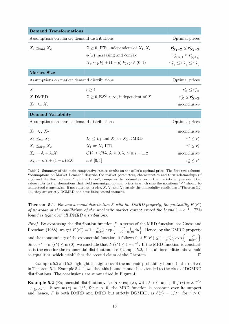
Demand Transformations
Assumptions on market demand distributions Optimal prices
X1 �mrd X2 Z ≥ 0, IFR, independent of X1, X2 r∗X1+Z ≤ r∗X2+Z
φ (x) increasing and convex r∗φ(X1) ≤ r∗φ(X2)
Xp ∼ pF1 + (1− p)F2, p ∈ (0, 1) r∗X1≤ r∗Xp
≤ r∗X2
Market Size
Assumptions on market demand distributions Optimal prices
X c ≥ 1 r∗X ≤ r∗cXX DMRD Z ≥ 0,EZ2 <∞, independent of X r∗X ≤ r∗X+Z
X1 �st X2 inconclusive
Demand Variability
Assumptions on market demand distributions Optimal prices
X1 �cx X2 inconclusive
X1 �ew X2 L1 ≤ L2 and X1 or X2 DMRD r∗1 ≤ r∗2X1 �disp X2 X1 or X2 IFR r∗1 ≤ r∗2Xi := δi + λiX CV1 ≤ CV2, δi ≥ 0, λi > 0, i = 1, 2 inconclusive
Xκ := κX + (1− κ)EX κ ∈ [0, 1] r∗κ ≤ r∗
Table 2. Summary of the main comparative statics results on the seller’s optimal price. The first two columns,“Assumptions on Market Demand” describe the market parameters, characteristics and their relationships (ifany) and the third column, “Optimal Prices”, compares the optimal prices in the markets in question. Boldvalues refer to transformations that yield non-unique optimal prices in which case the notationa “≤” should beunderstood elementwise. If not stated otherwise, X,X1 and X2 satisfy the unimodality conditions of Theorem 3.2,i.e., they are strictly DGMRD and have finite second moment.
Theorem 5.1. For any demand distribution F with the DMRD property, the probability F (r∗)of no-trade at the equilibrium of the stochastic market cannot exceed the bound 1 − e−1. Thisbound is tight over all DMRD distributions.
Proof. By expressing the distribution function F in terms of the MRD function, see Guess and
Proschan (1988), we get F (r∗) = 1− m(0)m(r∗) exp
{−∫ r∗
01
m(u)du}
. Hence, by the DMRD property
and the monotonicity of the exponential function, it follows that F (r∗) ≤ 1− m(0)m(r∗) exp
{− r∗
m(r∗)
}.
Since r∗ = m (r∗) ≤ m (0), we conclude that F (r∗) ≤ 1− e−1. If the MRD function is constant,as is the case for the exponential distribution, see Example 5.2, then all inequalities above holdas equalities, which establishes the second claim of the Theorem.
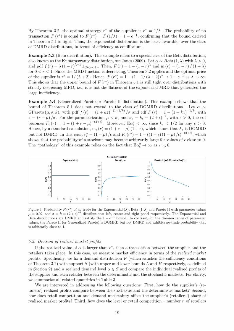
Examples 5.2 and 5.3 highlight the tightness of the no-trade probability bound that is derivedin Theorem 5.1. Example 5.4 shows that this bound cannot be extended to the class of DGMRDdistributions. The conclusions are summarized in Figure 4.
Example 5.2 (Exponential distribution). Let α ∼ exp (λ), with λ > 0, and pdf f (r) = λe−λr
1{0≤r<∞}. Since m (r) = 1/λ, for r > 0, the MRD function is constant over its supportand, hence, F is both DMRD and IMRD but strictly DGMRD, as ` (r) = 1/λr, for r > 0.
18
By Theorem 3.2, the optimal strategy r∗ of the supplier is r∗ = 1/λ. The probability of notransaction F (r∗) is equal to F (r∗) = F (1/λ) = 1 − e−1, confirming that the bound derivedin Theorem 5.1 is tight. Thus, the exponential distribution is the least favorable, over the classof DMRD distributions, in terms of efficiency at equilibrium.
Example 5.3 (Beta distribution). This example refers to a special case of the Beta distribution,also known as the Kumaraswamy distribution, see Jones (2009). Let α ∼ Beta (1, λ) with λ > 0,and pdf f (r) = λ (1− r)λ−1 1{0<r<1}. Then, F (r) = 1− (1− r)λ and m (r) = (1− r) / (1 + λ)for 0 < r < 1. Since the MRD function is decreasing, Theorem 3.2 applies and the optimal priceof the supplier is r∗ = 1/ (λ+ 2). Hence, F (r∗) = 1 − (1− 1/ (λ+ 2))λ → 1 − e−1 as λ → ∞.This shows that the upper bound of F (r∗) in Theorem 5.1 is still tight over distributions withstrictly decreasing MRD, i.e., it is not the flatness of the exponential MRD that generated thelarge inefficiency.
Example 5.4 (Generalized Pareto or Pareto II distribution). This example shows that thebound of Theorem 5.1 does not extend to the class of DGMRD distributions. Let α ∼GPareto (µ, σ, k), with pdf f (r) = (1 + kz)−(1+1/k) /σ and cdf F (r) = 1 − (1 + kz)−1/k, withz = (r − µ) /σ. For the parametrization µ < σε and σε = kε = (2 + ε)−1, with ε > 0, the cdf
becomes Fε (r) = 1 − (1 + r − µ)−(2+ε). Moreover, Eα2ε < ∞, since kε < 1/2 for any ε > 0.
Hence, by a standard calculation, mε (r) = (1 + r − µ) (1 + ε), which shows that Fε is DGMRD
but not DMRD. In this case, r∗ε = (1− µ) /ε and Fε (r∗) = 1− ((1 + ε) (1− µ) /ε)−(2+ε), whichshows that the probability of a stockout may become arbitrarily large for values of ε close to 0.The “pathology” of this example relies on the fact that Eα2
ε →∞ as ε↘ 0.
Figure 4. Probability F (r∗) of no-trade for the Exponential (λ), Beta (1, λ) and Pareto II with parameter valuesµ = 0.02, and σ = k = (2 + ε)−1 distributions: left, center and right panel respectively. The Exponential andBeta distributions are DMRD and satisfy the 1 − e−1 bound. In contrast, for the choosen range of parametervalues, the Pareto II (or Generalized Pareto) is DGMRD but not DMRD and exhibits no-trade probability thatis arbitrarily close to 1.
5.2. Division of realized market profits
If the realized value of α is larger than r∗, then a transaction between the supplier and theretailers takes place. In this case, we measure market efficiency in terms of the realized marketprofits. Specifically, we fix a demand distribution F (which satisfies the sufficiency conditionsof Theorem 3.2) with support S (with upper and lower bounds L and H respectively, as definedin Section 2) and a realized demand level α ∈ S and compare the individual realized profits ofthe supplier and each retailer between the deterministic and the stochastic markets. For clarity,we summarize all related quantities in Table 3.
We are interested in addressing the following questions: First, how do the supplier’s (re-tailers’) realized profits compare between the stochastic and the deterministic market? Second,how does retail competition and demand uncertainty affect the supplier’s (retailers’) share ofrealized market profits? Third, how does the level or retail competition – number n of retailers
19

Upstream Demand for the Supplier
Uncertain α ∼ F Deterministic α
Equilibriumwholesale price
r∗ = mF (r∗) r∗ = α/2
Realized Profits at Equilibrium
Supplier ΠUs = n
n+1r∗ (α− r∗)+ ΠD
s = nn+1 (α/2)2
Retailer i ΠUi = 1
(n+1)2(α− r∗)2
+ ΠDi = 1
(n+1)2(α/2)2
Aggregate ΠUAgg = ΠU
s +∑n
i=1 ΠUi ΠD
Agg = ΠUs +
∑ni=1 ΠU
i
Table 3. Wholesale price and realized profits in equilibrium for the stochastic (left column) and the deterministic(right column) markets. The realized equilibrium profits correspond to fixed demand level α ∈ S.
– affect supplier’s profits in both markets? The answers are summarized in Theorem 5.5 whichfollows rather immediately from Table 3. To avoid technicalities, we assume throughout thatthe upper bound H of the support S is large enough, so that H > 2r∗ (e.g., H =∞).
Theorem 5.5. Let F denote a demand distribution with support S within L and H, r∗ therespective optimal wholesale price in the stochastic market such that H > 2r∗, and α ∈ S, withα > r∗, a realized demand level, for which trading between supplier and retailers takes placein both the stochastic and the deterministic market. Let, also, ΠU
s /ΠUAgg and ΠD
s /ΠDAgg denote
the supplier’s share of realized profits in the stochastic and deterministic markets respectively.Then,
(i) ΠUs ≤ ΠD
s , with equality only for α = 2r∗. In particular, ΠUs /Π
Ds = 4 (r∗/α) (1− r∗/α)
for any α > r∗.(ii) ΠU
s /ΠUAgg decreases in the realized demand level α.
(iii) ΠDs /Π
DAgg is independent of the demand level α.
(iv) ΠUs /Π
UAgg is higher than ΠD
s /ΠDAgg for values of α ∈ (r∗, 2r∗), equal for α = 2r∗, and lower
otherwise.(v) ΠD
s /ΠDAgg and ΠU
s /ΠUAgg both increase in the level n of retail competition.
Finally, each retailer’s profit in the stochastic market, ΠUi , is strictly higher than her profit in
the deterministic market ΠDi for all demand levels α > 2r∗ and less otherwise, with equality for
α = 2r∗ only.
Proof. By Table 3, we have that: (i) ΠUs ≤ ΠD
s if and only if nn+1r
∗ (α− r∗)+ ≤nn+1 (α/2)2
which holds with strict inequality for all values of α, except for α = 2r∗ for which the quan-
tities are equal. The second part of statement (i) is immediate. For (ii)(ΠUs
)/(
ΠUAgg
)=
(nr∗ + r∗) / (nr∗ + α), and for (iii)(ΠDs
)/(
ΠDAgg
)= (n+ 1) / (n+ 2). Now, (iv) and (v) di-
rectly follow from the previous calculations. Finally, ΠUi ≥ ΠD
i if and only if 1(n+1)2
((α− r∗)+
)2 ≥1
(n+1)2(α/2)2 which holds with strict inequality for all values of α > 2r∗ and with equality for
α = 2r∗.
The statements of Theorem 5.5 are rather intuitive and in their largest part, with theexception of part (iv), they conform to earlier findings (Ai et al., 2012). (i) The supplier isalways better off if he is informed about the retail demand level. (ii) In the stochastic market,
20

he captures a larger share of the realized market profits for lower values of realized demand(but not lower than the no-trade threshold of r∗) whereas in the deterministic market (iii) hisshare of profits is constant with respect to the demand level. (iv) Yet, in the stochastic market,there exists an interval of demand realizations, namely (r∗, 2r∗), for which the supplier’s profits(although less than in the deterministic market) represent a larger share of the aggregate marketprofits. In any case, (v) retail competition benefits the supplier. Finally, in the case that thesupplier prices under uncertainty, each retailer makes a larger profit for higher realized demandvalues which abides to intuition. These observations conform with the existence of conflictingincentives regarding demand-information disclosure between the retailers and the supplier, cf.Li and Petruzzi (2017).
5.2.1. Deterministic and stochastic markets: aggregate profits
We next turn to the comparison of the aggregate market profits between the deterministicand the stochastic market. As before, we fix a demand distribution F (which is again assumed tosatisfy the sufficiency conditions of Theorem 3.2) with support S within L and H, and evaluatethe ratio ΠU
Agg/ΠDAgg of the aggregate realized market profits in the stochastic market to the
aggregate market profits in the deterministic market. To study market performance underthe two scenarios, we need to evaluate the combined effect of demand uncertainty and retailcompetition. For a realized demand α ≤ r∗, there is a stockout and the realized aggregatedprofits ΠU
Agg are equal to 0. In this case, the stochastic market performs arbitrarily worse thanthe deterministic market and the ratio is equal to 0 for any number n ≥ 1 of competing retailers.Hence, for a non-trivial analysis, we restrict attention to α > r∗ for which trading takes placein both the stochastic and the deterministic markets.
Theorem 5.6. Let F denote a demand distribution with support S within L and H, with Hlarge enough, and let r∗ denote the respective optimal wholesale price in the stochastic market.Additionally, suppose that α ∈ S, with α > r∗ is a realized demand level for which tradingbetween supplier and retailers takes place in both the stochastic and the deterministic market.Let, also, ΠU
Agg/ΠDAgg denote the ratio of the aggregate realized profits in the stochastic market
to the aggregate profits in the deterministic market. Then,
(i) ΠUAgg/Π
DAgg > 1 for α > 2r∗ if n = 1 or n = 2 and for α ∈
(2r∗, 2n
n−2r∗)
if n ≥ 3.
(ii) ΠUAgg/Π
DAgg is maximized for α∗ = 2nr∗/ (n− 1) for n ≥ 2, for which it is equal to 1 +
(n (n+ 2))−1. Moreover, ΠUAgg/Π
DAgg converges to 4/ (n+ 2) as α→∞ for any n ≥ 1.
(iii) ΠUAgg/Π
DAgg increases in the level of competition for demand levels α < 2r∗ and decreases
thereafter.
Again, to avoid unnecessary technicalities in the proof of Theorem 5.6, we assume that His large enough, e.g., H =∞.
Proof. By Table 3, a direct substitution yields that ΠUAgg −ΠD
Agg > 0 iff
2− n4· α2 + r∗ (n− 1)α− n (r∗)2 > 0
with α > r∗. For n = 1, 2, the result is straightforward, whereas for n ≥ 3 the result followsfrom the observation that the roots of the expression in the left part are given by α1,2 =2r∗ · n−1±1
n−2 . This establishes (i) and after some trivial algebra, also (ii). To obtain (iii), we
compare ΠUAgg/Π
DAgg for arbitrary n to ΠU
Agg/ΠDAgg for n+ 1
4 (α− r∗) (α+ (n+ 1) r∗)
α2 (n+ 3)>
4 (α− r∗) (α+ nr∗)
α2 (n+ 2)⇐⇒ 2r∗ > α
which yields the statement.
21

Statement (i) of Theorem 5.6 asserts that there exists an interval of realized demand values,whose upper bound depends on the number n of competing retailers, for which the stochasticmarket outperforms the deterministic market in terms of aggregate profits. The effect of in-creasing retail competition on the aggregate profits of the stochastic market is twofold. First,the range (interval) of demand values for which the ratio of aggregate profits exceeds 1 reducesto a single point as competition increases (n → ∞). Second, for larger values of realized de-mand, the ratio converges to 4/ (n+ 2) as α→∞. This shows that uncertainty on the side ofthe supplier is less detrimental for the aggregate market profits when the level of retail compe-tition is low. In particular, for n = 1, 2, the aggregate profits of the stochastic market remainstrictly higher than the profits of the deterministic market for all large enough realized demandlevels. As competition increases this remains true only for lower (but still above the no-tradethreshold) demand levels. However, for higher demand realizations, the ratio degrades linearlyin the number of competing retailers.
The statements of Theorem 5.6 are illustrated in Figure 5. Here α ∼ Gamma (2, 2) but thepicture is essentially the same for any choice of demand distribution that satisfies the sufficiencyconditions of Theorem 3.2 and for which H is large enough, i.e., H > 2r∗.
Figure 5. The left panel depicts the ratio ΠUAgg/Π
DAgg for n = 2, 5 and 8, where α ∼ Gamma (2, 2). The dashed
line shows the points α = 2nr∗/ (n− 1) in which the ratios are maximized, taking the value 1 + (n (n+ 2))−1.The right panel magnifies the interval [4, 7] around the intersection point α = 2r∗ of the three curves. The ratioincreases in n prior to the intersection point, 2r∗ ≈ 5.657, and decreases in n thereafter.
6. Conclusions
In this paper, we revisited the classic problem of optimal pricing by a monopolist who isfacing linear stochastic demand. The monopolist may sell directly to the consumers or via aretail market with an arbitrary competition structure. Our main theoretical finding is thatthe price elasticity of expected demand, and hence also the monopolist’s optimal prices, can beexpressed in terms of the mean residual demand (MRD) function of the demand distribution. Ineconomic terms, the MRD function describes the expected additional demand given that currentdemand has reached or exceeded a certain threshold. This leads to a closed form characterizationof the points of unitary elasticity that maximize the monopolist’s profits and the derivation of amild unimodality condition for the monopolist’s objective function that generalizes the widelyused increasing generalized failure rate (IGFR) condition. A direct byproduct is a distributionfree and tight bound on the probability of no trade between the supplier and the retailers.
When we compare optimal prices between markets with different demand characteristics,the main implication of the above characterization is that it allows us to exploit various formsof knowledge on the demand distribution via the theory of stochastic orderings. Specifically, iftwo markets can be ordered in terms of their mean residual demand function, then the seller’soptimal prices can be ordered accordingly. This establishes a link between the price elasticityof expected demand, which is naturally the critical determinant of price movements in responseto changes in demand, and some well-understood characteristics of the demand distribution.
22

The stochastic orders approach works under various informational assumptions on the demanddistribution and provides a way to systematically exploit the abundance of data that firmspossess about historical price/demand.
From a managerial perspective, our study provides a tractable theoretical framework whichcan be used to reason about price changes in advance of anticipated market movements or tobenchmark data-driven predictions that are derived from pricing analytics. Our results suggestthat the effects of market size and demand variability on prices critically depend on the notionsof size and variability that will be employed. This implies that exact predictions about pricemovements can only be done in a case by case basis and should only be used with caution. Suchtools are particularly useful in industries in which fixing a price often precedes the demandrealization such as subscription based businesses or businesses that sell durable goods, ticketsor leisure time services. More generally, our findings can be used to explain the diversity ofprice responses to market characteristics that are observed in practice and provide a diversetoolbox for managers to optimally set and adjust prices under different market conditions.
Acknowledgements
Stefanos Leonardos gratefully acknowledges support by the Alexander S. Onassis PublicBenefit Foundation and partial support by NRF 2018 Fellowship NRF-NRFF2018-07.
References
X. Ai, J. Chen, and J. Ma. Contracting with demand uncertainty under supply chain competi-tion. Annals of Operations Research, 201(1):17–38, Dec 2012. doi:10.1007/s10479-012-1227-x.
M. Bagnoli and T. Bergstrom. Log-concave probability and its applications. Economic Theory,26(2):445–469, 2005. doi:10.1007/s00199-004-0514-4.
M. Banciu and P. Mirchandani. Technical note – new results concerning probability distri-butions with increasing generalized failure rates. Operations Research, 61(4):925–931, 2013.doi:10.1287/opre.2013.1198.
F. Belzunce, C. Martınez-Riquelme, and J.M. Ruiz. On sufficient conditions for mean resid-ual life and related orders. Computational Statistics & Data Analysis, 61:199–210, 2013.doi:10.1016/j.csda.2012.12.005.
F. Belzunce, C. Martinez-Riquelme, and J. Mulero. Chapter 2: Univariate stochastic orders.In F. Belzunce, C. Martınez-Riquelme, and J. Mulero, editors, An Introduction to StochasticOrders, pages 27 – 113. Academic Press, 2016. doi:10.1016/B978-0-12-803768-3.00002-8.
G. Berbeglia, G. Rayaprolu, and A. Vetta. Pricing policies for selling indivisible storablegoods to strategic consumers. Annals of Operations Research, 274(1):131–154, Mar 2019.doi:10.1007/s10479-018-2916-x.
F. Bernstein and A. Federgruen. Decentralized Supply Chains with Competing Retailers UnderDemand Uncertainty. Management Science, 51(1):18–29, 2005. doi:10.1287/mnsc.1040.0218.
D. Bradley and R. Gupta. Limiting behaviour of the mean residual life. Annals of the Instituteof Statistical Mathematics, 55(1):217–226, 2003. doi:10.1007/BF02530495.
F. Y. Chen, H. Yan, and L. Yao. A newsvendor pricing game. IEEE Transactions onSystems, Man, and Cybernetics - Part A: Systems and Humans, 34(4):450–456, 2004.doi:10.1109/TSMCA.2004.826290.
H. Chen, M. Hu, and G. Perakis. Distribution-Free Pricing. Mimeo, Available at SSRN, 2017.
23

L. Chen, G. Nan, and M. Li. Wholesale Pricing or Agency Pricing on Online Retail Platforms:The Effects of Customer Loyalty. International Journal of Electronic Commerce, 22(4):576–608, 2018. doi:10.1080/10864415.2018.1485086.
M. C. Cohen, G. Perakis, and R. S. Pindyck. Pricing with Limited Knowledge of Demand. InProceedings of the 2016 ACM Conference on Economics and Computation, EC ’16, page 657,2016. doi:10.1145/2940716.2940734.
L. Colombo and P. Labrecciosa. A note on pricing with risk aversion. European Journal ofOperational Research, 216(1):252–254, 2012. ISSN 0377-2217. doi:10.1016/j.ejor.2011.07.027.
J.D. Dana. Monopoly price dispersion under demand uncertainty. International EconomicReview, 42(3):649–670, 2001. URL http://www.jstor.org/stable/827024.
D. De Wolf and Y. Smeers. A Stochastic Version of a Stackelberg-Nash-Cournot EquilibriumModel. Management Science, 43(2):190–197, 1997. doi:10.1287/mnsc.43.2.190.
L. Dong, X. Guo, and D. Turcic. Selling a Product Line Through a Retailer When Demand IsStochastic: Analysis of Price-Only Contracts. Manufacturing & Service Operations Manage-ment, 21(4):742–760, 2019. doi:10.1287/msom.2018.0720.
F. Guess and F. Proschan. Mean residual life: theory and applications. In P. R. Krishnaiahand C. R. Rao, editors, Quality Control and Reliability, volume 7 of Handbook of Statistics,pages 215–224. Elsevier Amsterdam, 1988. doi:10.1016/S0169-7161(88)07014-2.
W. Hall and J. Wellner. Mean residual life. In M. Csørgø, D. A. Dawson, J. N. K. Rao, andA. K. Md. E. Saleh, editors, Proceedings of the International Symposium on Statistics andRelated Topics, pages 169–184. North Holland Amsterdam, 1981.
M. Harris and A. Raviv. A Theory of Monopoly Pricing Schemes with Demand Uncertainty.The American Economic Review, 71(3):347–365, 1981. doi:10.2307/1802784.
J. Huang, M. Leng, and M. Parlar. Demand functions in decision modeling: A com-prehensive survey and research directions. Decision Sciences, 44(3):557–609, 2013.doi:10.1111/deci.12021.
W. Hwang, N. Bakshi, and V. DeMiguel. Wholesale Price Contracts for Reliable Supply.Production and Operations Management, 27(6):1021–1037, 2018. doi:10.1111/poms.12848.
C. Jones. Kumaraswamy’s distribution: A beta-type distribution with some tractability advan-tages. Statistical Methodology, 6:70–81, 2009. doi:10.1016/j.stamet.2008.04.001.
A. Kocabıyıkoglu and I. Popescu. An Elasticity Approach to the Newsvendor with Price-Sensitive Demand. Operations Research, 59(2):301–312, 2011. doi:10.1287/opre.1100.0890.
C. Koki, S. Leonardos, and C. Melolidakis. Comparative Statics via Stochastic Orderings in aTwo-Echelon Market with Upstream Demand Uncertainty, pages 331–343. Springer Interna-tional Publishing, Cham, 2018. doi:10.1007/978-3-030-00473-6 36.
P. Kouvelis, G. Xiao, and N. Yang. On the Properties of Yield Distributions in Random YieldProblems: Conditions, Class of Distributions and Relevant Applications. Production andOperations Management, 27(7):1291–1302, 2018. doi:10.1111/poms.12869.
H. Krishnan. A note on demand functions with uncertainty. Operations Research Letters, 38(5):436–440, 2010. doi:10.1016/j.orl.2010.06.001.
24
G.J. Kyparisis and C. Koulamas. The price-setting newsvendor with nonlinear sal-vage revenue and shortage cost. Operations Research Letters, 46(1):64–68, 2018.doi:10.1016/j.orl.2017.11.001.
C.-D. Lai and M. Xie. Stochastic Ageing and Dependence for Reliability. Springer Science +Business Media, Inc., 2006.
M.A. Lariviere. Supply Chain Contracting and Coordination with Stochastic Demand. InS. Tayur, R. Ganeshan, and M. Magazine, editors, Quantitative Models for Supply ChainManagement, pages 233–268. Springer US, Boston, MA, 1999. doi:10.1007/978-1-4615-4949-9 8.
M.A. Lariviere. A Note on Probability Distributions with Increasing Generalized Failure Rates.Operations Research, 54(3):602–604, 2006. doi:10.1287/opre.1060.0282.
M.A. Lariviere and E. Porteus. Selling to the Newsvendor: An Analysis of Price-Only Contracts. Manufacturing & Service Operations Management, 3(4):293–305, 2001.doi:10.1287/msom.3.4.293.9971.
S. Leonardos and C. Melolidakis. A Class of Distributions for Linear Demand Markets. arXive-prints, 2020. URL https://arxiv.org/abs/1805.06327.
S. Leonardos and C. Melolidakis. On the Equilibrium Uniqueness in Cournot Competition withDemand Uncertainty. The B.E. Journal of Theoretical Economics, 20(2):20190131, 2020a.doi:10.1515/bejte-2019-0131.
S. Leonardos and C. Melolidakis. Endogenizing the Cost Parameter in Cournot Oligopoly.International Game Theory Review, 22(02):2040004, 2020b. doi:10.1142/S0219198920400046.
S. Leonardos and C. Melolidakis. On the Mean Residual Life of Cantor-Type Distributions:Properties and Economic Applications. Austrian Journal of Statistics, 50(4):65–77, 2021.doi:10.17713/ajs.v50i4.1118.
M. Li and N.C. Petruzzi. Technical Note–Demand Uncertainty Reduction in Decen-tralized Supply Chains. Production and Operations Management, 26(1):156–161, 2017.doi:10.1111/poms.12626.
Q. Li and D. Atkins. On the effect of demand randomness on a price/quantity setting firm. IIETransactions, 37(12):1143–1153, 2005. doi:10.1080/07408170500288182.
A. L. Lopez and X. Vives. Overlapping Ownership, R&D Spillovers, and Antitrust Policy.Journal of Political Economy, 127(5):2394–2437, 2019. doi:10.1086/701811.
S. Luo, S.P. Sethi, and R. Shi. On the optimality conditions of a pricesetting newsvendor problem. Operations Research Letters, 44(6):697–701, 2016.doi:https://doi.org/10.1016/j.orl.2016.08.005.
P. Mandal, R. Kaul, and T. Jain. Stocking and pricing decisions under endogenous demandand reference point effects. European Journal of Operational Research, 264(1):181–199, 2018.doi:10.1016/j.ejor.2017.05.053.
C. Melolidakis, S. Leonardos, and C. Koki. Measuring Market Performance with Stochastic De-mand: Price of Anarchy and Price of Uncertainty. In S. Destercke, T. Denoeux, F. Cuzzolin,and A. Martin, editors, Belief Functions: Theory and Applications, pages 163–171, Cham,2018. Springer International Publishing. doi:10.1007/978-3-319-99383-6 21.
25

E.S. Mills. Uncertainty and price theory. The Quarterly Journal of Economics, 73(1):116–130,1959.
S. P. Mukherjee and A. Chatterjee. Closure under convolution of dominance relations. CalcuttaStatistical Association Bulletin, 42(3-4):251–254, 1992. doi:10.1177/0008068319920309.
S. P. Mukherjee and Aditya Chatterjee. On Some Closure Properties of Dominance RelationsBetween Life Distributions Based on Reliability Measures. Calcutta Statistical AssociationBulletin, 40(1–4):325–342, 1990. doi:10.1177/0008068319900525.
V. Padmanabhan and I.P.L. Png. Manufacturer’s Return Policies and Retail Competition.Marketing Science, 16(1):81–94, 1997. doi:10.1287/mksc.16.1.81.
A. Paul. A Note on Closure Properties of Failure Rate Distributions. Operations Research, 53(4):733–734, 2005. doi:10.1287/opre.1040.0206.
G. Perakis and G. Roels. The Price of Anarchy in Supply Chains: Quantifyingthe Efficiency of Price-Only Contracts. Management Science, 53(8):1249–1268, 2007.doi:10.1287/mnsc.1060.0656.
N.C. Petruzzi and M. Dada. Pricing and the Newsvendor Problem: A Review with Extensions.Operations Research, 47(2):183–194, 1999. doi:10.1287/opre.47.2.183.
J. Riley and R. Zeckhauser. Optimal Selling Strategies: When to Haggle, When to Hold Firm.The Quarterly Journal of Economics, 98(2):267–289, 05 1983. doi:10.2307/1885625.
J. Rubio-Herrero and M. Baykal-Gursoy. On the unimodality of the price-setting newsvendorproblem with additive demand under risk considerations. European Journal of OperationalResearch, 265(3):962–974, 2018. doi:10.1016/j.ejor.2017.08.055.
M. Shaked and G. Shanthikumar. Stochastic Orders. Springer Series in Statistics, New York,2007. ISBN 0-387-32915-3.
M. Shaked and J. G. Shanthikumar. Dynamic Multivariate Mean Residual Life Functions.Journal of Applied Probability, 28(3):613–629, 1991.
N. Singh and X. Vives. Price and Quantity Competition in a Differentiated Duopoly. The RANDJournal of Economics, 15(4):546–554, 1984. URL http://www.jstor.org/stable/2555525.
S. K. Singh and G. S. Maddala. A Function for Size Distribution of Incomes. Econometrica, 44(5):963–70, 1976. doi:10.2307/1911538.
Y. Song, S. Ray, and S. Li. Structural Properties of Buyback Contracts for Price-Setting Newsvendors. Manufacturing & Service Operations Management, 10(1):1–18, 2008.doi:10.1287/msom.1060.0140.
Y. Song, S. Ray, and T. Boyaci. Technical Note – Optimal Dynamic Joint Inventory-PricingControl for Multiplicative Demand with Fixed Order Costs and Lost Sales. Operations Re-search, 57(1):245–250, 2009. doi:10.1287/opre.1080.0530.
R.K. Tyagi. On the Effects of Downstream Entry. Management Science, 45(1):59–73, 1999.doi:10.1287/mnsc.45.1.59.
G.J. Van den Berg. On the uniqueness of optimal prices set by monopolistic sellers. Journal ofEconometrics, 141(2):482–491, 2007. doi:10.1016/j.jeconom.2006.10.005.
26

C.-H. Wu, C.-W. Chen, and C.-C. Hsieh. Competitive pricing decisions in a two-echelon supplychain with horizontal and vertical competition. International Journal of Production Eco-nomics, 135(1):265–274, 2012. doi:10.1016/j.ijpe.2011.07.020. Advances in Optimization andDesign of Supply Chains.
M. Xu, Y.(F.) Chen, and X. Xu. The effect of demand uncertainty in a price-settingnewsvendor model. European Journal of Operational Research, 207(2):946–957, 2010.doi:10.1016/j.ejor.2010.06.024.
W. Xue, J. Zuo, and X. Xu. Analysis of market competition and information asymmetry onselling strategies. Annals of Operations Research, 257(1):395–421, 2017. doi:10.1007/s10479-015-1809-5.
S.-L. Yang and Y.-W. Zhou. Two-echelon supply chain models: Considering duopolistic retail-ers’ different competitive behaviors. International Journal of Production Economics, 103(1):104–116, 2006. doi:10.1016/j.ijpe.2005.06.001.
L. Yao, Y.(F.) Chen, and H. Yan. The newsvendor problem with pricing: Extensions. In-ternational Journal of Management Science and Engineering Management, 1(1):3–16, 2006.doi:10.1080/17509653.2006.10670993.
T. Ye and H. Sun. Price-setting newsvendor with strategic consumers. Omega, 63:103–110,2016. ISSN 0305-0483. doi:10.1016/j.omega.2015.10.006.
27