monte carlo solution for actuarial problems - member · monte carlo solution for actuarial problems...

RECORD OF SOCIETY OF ACTUARIES 1995 VOL. 21 NO. 3A

MONTE CARLO SOLUTION FOR ACTUARIAL PROBLEMS

Instructor: ANDREW F. SEILA*

The teaching session reexamines Monte Carlo solution for actuarial problems.

MR. ANDREW F. SEILA: I 'm Andy Seila and I 'm a professor of management science at the University of Georgia. Before we get started, I would like to poll the audience. How many of you have used simulation to solve some sort &actuarial problem in practice? That looks like perhaps 60-70% of you. I would conclude that simulation is a tool that is commonly used in the day-to-day course of actuarial analysis.

I noticed that the theme of this meeting is, in a word, professionalism. I spent some time thinking about how the topic &simulation fits with that theme and I realized that it fits quite well. Let me explain. Any time an actuary performs an analysis, it must be judged by the standards of the profession. In other words, the work you do must be able to stand up to criticism by others--management, regulators and consumers. Thus, it is not sufficient to just do a simulation analysis; the analysis must be above reproach. It must be defensible. In this session, I want to talk about simulation methods and generally accepted standards for applying those methods in practice.

Our objectives are three: to survey some basic simulation methods and indicate what tools and techniques are used when simulation is applied to solve a problem; to show that simulation is an all-purpose tool for problem solving if the problem involves analyzing a model; and finally to alert you to some potential dangers when using simulation. In this last category, I will caution you concerning the random number generator you use and also discuss concerns with output data analysis.

SIMULATION VERSUS MATHEMATICAL ANALYSIS First, I would like to define what I mean by simulation and compare it to other techniques for model analysis. Monte Carlo simulation is a collection of techniques to extract information from a stochastic model. We have a stochastic model and we want to use that model to tell us something about the system that it represents. Simulation provides some techniques, based on sampling the behavior of the model, to provide this information. Mathematical analysis is another method to extract information from a stochastic model. So, simulation and mathematical analysis work to achieve the same goals, but their approaches differ. Let's illustrate this idea using an example.

For our example, consider a simple aggregate claims model, where Yis the aggregate claims, N is the number of claims received in a month and X~, X2, and so on are the claim amounts for individual claims. Further, assume that N has a Poisson distribution with mean 10.0. Then, the mean number of claims per month is ten and the variance is also ten.

N r=Ex,

i=1

*Mr. Seila, not a member of the sponsoring organizations, is a Professor of Management Science at the University of Georgia in Athens, GA.

327

RECORD, VOLUME 21

Also, assume that claim amounts have a lognormal distribution with parameters/z=0.7 and o2=-1.80. Claim amounts are expressed in units of thousands of dollars. Then, the mean, variance and standard deviation of the individual claim amounts are 4.95, 123.88, and 11.13, respectively. The following example shows how these were calculated.

i i 2 k t * - -

E(X)=e 2 = 4.95 Var(X) = e 2u +O2(e o2_ 1 ) = 123.88

o(X) = ~ ( X ) = 11.13

Suppose that we want to get the following information from the model: 1. Mean of total claims, which we denote by E(Y); 2. Variance of total claims, or Vat (Y); and 3. 90th percentile of total claims, denoted by ~.9(Y)

First, let's consider the mathematical approach. This method uses probability theory to compute the parameters. The first two are easy to compute from the first two moments of the individual claims distributions and the number of claims per month. The calculations are shown in the example that follows. So, the mean of the aggregate claims is $49.53 in units of thousands of dollars, and the variance is 1,484.12. We can take the square root of this to get the standard deviation of 38.52. These calculations were easy. But, what about the 90th percentile of the distribution of aggregate claims? The entire distribution of Y must be known to compute this parameter. Actually, I understand that this parameter can be computed for this particular model using some techniques by Gordon Willmot and Harry Panjer. Let's just say that if it can be done mathematically, it depends generally upon the specific distributions involved and the calculations will be difficult and tedious.

E(Y) =E(N)E(X) =(10.0)(4.95) = 49.53 Var(r3--Var(~[E(X)]: +E(.,V)Var(X)

=(10.0)(4.95)2+(10.0)(123.88)=1,484.12

o(Y)=~,484.12=38.52 But...

~b.9(Y)=?

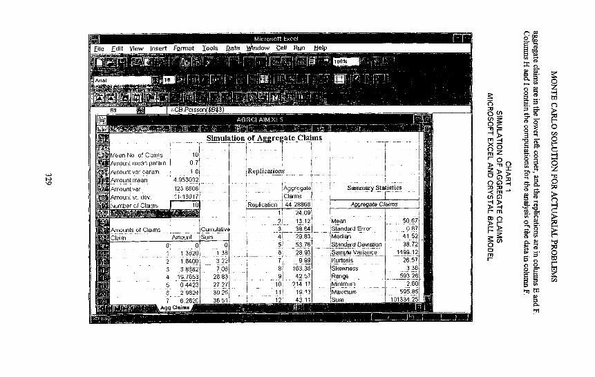
The simulation approach samples observations of Y and computes estimates of the parameters we want to know using these observations. I have implemented the simulation using a spreadsheet, Microsoft Excel, with a simulation add-in package, Crystal Ball that implements some simulation capabilities. With the simulation approach, we would proceed as follows: first, sample N, the monthly number of claims, from a Poisson distribution with mean 10.0. Next, sample each of the N claim amounts from a lognormal distribution with parameters 0.7-1.80. Now, add the claim amounts to get the aggregate claims for the month. We repeat these three steps 2,000 times (independently) to produce a sample of 2,000 observations of aggregate claims.

Chart 1 is a screen shot of this model implemented using Microsoft Excel and Crystal Ball. I'll comment a little more about spreadsheet add-ins for simulation a little later. In this model, we see all of the parameters in the upper left comer. The cell containing the aggregate claims for one replication is cell B-10, which is shaded. The calculations for the

328

pile Edit V iew inser t Format ] [ools ~ a t a

Ariel

_O~ll Rl/n Help

8~ ]~i~l I =C8.Poisson($B$3)

Mean No of Claims Amount mean param

~nount vat param Amount mean

Amount var

Amount st dev

Number of Claims

S i m u l a t i o n o [ A g g r e g a t e C l a i m s , . . . . . . . . . . . . I

. . . . . . . . I . . . . . . . . . . . . . . i . . . . . . . . . . . 1 , 10 I l i O7 I , ] I 8 ~Rephcat,ons t : ]

4.95s03~ ~7 i . . . . . . , - . . . . . . / i . " . . . . [-

{ !Replicat, on , 4 :4 .2aod l F ~

, i ~4.o9 , l 1

Cumula[iva ~u;T; ......... I

Amounts of Claims Claim- . . . . . . . . . . . . . . ~T~ount

o 0 I !. _38_2_0 2 18400 s s.8382 4 19.7653 5 04423

7 6.2620

21 13.12 'Mean

Standard Deviation 5 ~.z6 ! . .~.7_2 /

. . . . . [ ~ u ~ & ~ . . . . . . . . . . . . . I - - ~ ' ~

9] " ~,2Sf Ra.~e I ._ 59s ?o

I ~ 2 -~:13 Ma~,~om 595.85 43.11, isum ~01s34 2Sl

o~

C~

r'-

o O i l l

°o= >o=> 6"~ --I

63

m

P

t~

8 ~

o

" O

~ g ,P--

~'F,"

!~ o

O Z # ¢3

©

,-]

'-tl ©

> ¢3

RECORD, VOLUME 21

Chart 2 shows the histogram of the aggregate claims data in column F of the spreadsheet. This graph was also produced using Microsoft Excel. We distribution is highly skewed, with a fairly heavy tail. Now we are ready to compute the characteristics of this distribution.

CHART 2 DISTRIBUTION OF AGGREGATE CLAIMS

¢J C

Cr .= U.

0 30 60 90 120 150 180 210 240 270 300 330 Aggregate Claims

This chart shows the computations for point estimates and confidence intervals for the three parameters we want to know. We point estimate for the mean is 50.67 in units of thousands of dollars, and the 95% confidence interval is 50.67 plus or minus 1.71.

This range includes the value we computed earlier using mathematical analysis, 49.53. Similarly, the point estimate and confidence interval for the variance are 1,499.12 and from 1,411.61-1,598.21, respectively. The formulas for computing this interval are shown in the following example. This range also includes the true value, 1484.12, which we computer earlier.

330


Estimate E(Y) by n

~ = 1 ~ = 50.67 F/ I= l

Confidence interval: T+Z s = 50.67q-1-71 [95%]

~ 2 - - v~

Estimate Vat (Y) by

1 s2= n-1 ~-= (Y"-Y)2 = 1'499'12

Confidence interval: (n-1)s 2 < VAR(Y) < (n-1)s2

1,411.61 < VAR(Y) < 1,598.21 [95%] 37.57 < o(F) < 39.98

Now, unlike the mathematical approach, we can also estimate the 90th percentile, or any other percentile, for that matter, of the distribution of aggregate claims. The computations are shown in the following example. We just find the sample 90th percentile, and use two other percentiles computed from the normal distribution to find the confidence limits. This nonparametric confidence interval is described in the textbook on mathematical statistics by Hogg and Craig, I believe. We see that the confidence interval is between 88.57-98.92. I believe this is a 95% confidence interval. Since we don't have an analytic way to compute this parameter, we can't be sure that the true percentile is in this range, but we can be fairly confident it is some value in here.

Estimate qb.9 by

YC.9,) where }'(1) <- YC2)-<'"-< Y~.)

Y0s000) = 95.58 Confidence interval: YCr) < d~.90 <Ycr') where

r = L.9n - ZI_ ~ ~ J and r ' = ].9n + Zt_ ~ ~ J

if n is large. Yo773) = 88.57 < qb.9 < 98.92 = Yos27) [95%]

Let's compare the simulation and analytical methods. First, mathematical analysis works for a limited number of parameters in a limited selection of models. Analysis needs a new technique for each new type of model or each new parameter. Thus, if you want to compute the same parameter for a new model or a new parameter for the same model, you will generally have to start from scratch and derive new formulas or algorithms to compute the parameter. Analysis also gives "exact" answers, given the model's assumptions. I put "exact" in quotes because the model often must be greatly simplified to allow analytical solutions to be applied. Mathematical methods usually involve less computation time. There are exceptions, but generally, it is true.

331

RECORD, VOLUME 21

On the other hand, simulation can produce only estimates of parameters since the technique works by sampling from the distributions in the model. As a result, simulation normally involves more computation time. However, simulation can be used to analyze models of much greater complexity than those that can be analyzed using the mathematical approach. Importantly, simulation uses exactly the same techniques to analyze all models, regardless of complexity. Thus, it is no problem to make the model more complex and more realistic, and then to compute estimates of the parameters you want to know using simulation. So, simulation can be used to analyze models too complex for mathematical treatment. This approach also can be used to estimate parameters that can't be computed analytically. If you use simulation, you do not need to be concerned with whether the model has been solved. Moreover, you use basically the same methods to analyze all models using simulation. You don't need a different bag of tools for each type of model; one set of tools works for all. As a bonus, simulation is almost always much easier to explain and demonstrate to management, so model solutions are easier to sell.

I am not trying to promote simulation as a replacement for mathematical methods. There are many models where the mathematical approach is preferred. What I am trying to say is that simulation is a method of very general applicability that can be applied to models that do not yield to mathematical analysis. The disadvantages of simulation are that it requires more computation time and the results are only estimates of parameters. Computation time is very inexpensive and expected to become even less expensive in the future, so the first disadvantage is rapidly disappearing. Frequently you want to know parameters only roughly, say, plus or minus 10%. In this case, exact values are of no more use than a confidence interval. Indeed, the error introduced by the simplifying assumptions in the model is often more than the sampling error of the estimators in the simulation. If the model must be further simplified to enable a mathematical solution, the solution may be precise but not accurate because it is a solution to a model that does not accurately represent the real system. Indeed, the error of approximation can't normally be determined. On the other hand, the sampling error can and should always be computed from the simulation.

So, we have a tradeoff: We can either simplify the model and make it less realistic so it can be solved mathematically for the parameters of interest, or we can keep the detail in the model but settle for estimates of the parameters. The choice here is, of course, a matter of your judgment. To illustrate this point, consider the aggregate claims model again. Let's compute the 90th percentile by treating aggregate claims as a normal random variable: (We know from the histogram of the simulation that this is not true, but it is a simplifying assumption.) The calculations are shown in the following example. From these computations, we get 98.84 as the approximation. If we compare this approximation to the confidence interval computed using simulation, we see that this value is just barely in the confidence interval. This gives us some confidence that the approximation is reasonable. That is, we computed the same parameter using simulation and an approximate mathematical method, and got values that agreed. This demonstrates another use for simulation--to validate analytical approximations.

Aggregate claims model revisited.

N

332


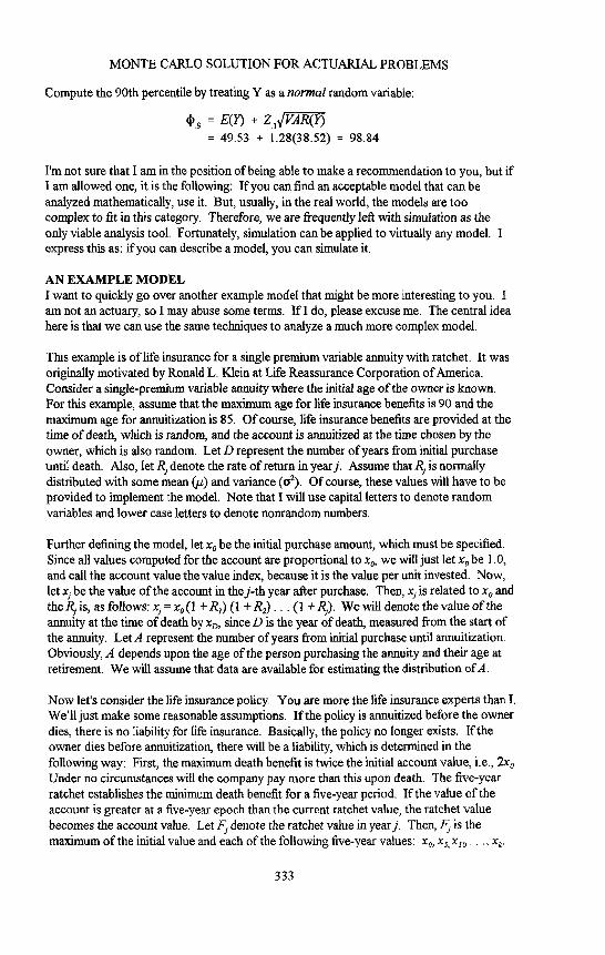
Compute the 90th percentile by treating Y as a n o r m a l random variable:

¢ , = E(r) + z , vA,[P-~ = 49.53 + 1.28(38.52) = 98.84

I'm not sure that I am in the position of being able to make a recommendation to you, but if I am allowed one, it is the following: If you can find an acceptable model that can be analyzed mathematically, use it. But, usually, in the real world, the models are too complex to fit in this category. Therefore, we are frequently left with simulation as the only viable analysis tool. Fortunately, simulation can be applied to virtually any model. I express this as: if you can describe a model, you can simulate it.

AN EXAMPLE MODEL I want to quickly go over another example model that might be more interesting to you. I am not an actuary, so I may abuse some terms. I f I do, please excuse me. The central idea here is that we can use the same techniques to analyze a much more complex model.

This example is of life insurance for a single premium variable annuity with ratchet. It was originally motivated by Ronald L. Klein at Life Reassurance Corporation of America. Consider a single-premium variable annuity where the initial age of the owner is known. For this example, assume that the maximum age for life insurance benefits is 90 and the maximum age for annuitization is 85. Of course, life insurance benefits are provided at the time of death, which is random, and the account is annuitized at the time chosen by the owner, which is also random. Let D represent the number of years from initial purchase until death. Also, let Rj denote the rate of return in yearj. Assume that Rj is normally distributed with some mean (/z) and variance (02"). Of course, these values will have to be provided to implement the model. Note that I will use capital letters to denote random variables and lower case letters to denote nonrandom numbers.

Further defining the model, let x o be the initial purchase amount, which must be specified. Since all values computed for the account are proportional to Xo, we will just let x o be 1.0, and call the account value the value index, because it is the value per unit invested. Now, let xj be the value of the account in thej-th year after purchase. Then, xj is related to x o and

the Rj is, as follows: xj = x o (1 + R~) (1 + Re) . . . (1 + Rj). We will denote the value of the annuity at the time of death by xD, since D is the year of death, measured from the start of the annuity. LetA represent the number of years from initial purchase until annuitization. Obviously, A depends upon the age of the person purchasing the annuity and their age at retirement. We will assume that data are available for estimating the distribution ofA.

Now let's consider the life insurance policy. You are more the life insurance experts than I. We'll just make some reasonable assumptions. If the policy is annuitized before the owner dies, there is no liability for life insurance. Basically, the policy no longer exists. If the owner dies before annuitization, there will be a liability, which is determined in the following way: First, the maximum death benefit is twice the initial account value, i.e., 2 x o

Under no circumstances will the company pay more than this upon death. The five-year ratchet establishes the minimum death benefit for a five-year period. If the value of the account is greater at a five-year epoch than the current ratchet value, the ratchet value becomes the account value. Let Fj denote the ratchet value in yearj. Then, Fj is the maximum of the initial value and each of the following five-year values: xo, xs, x ~ o . . . , xk.

333

RECORD, VOLUME 21

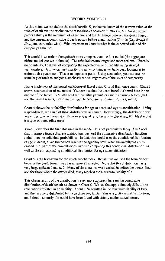
At this point, we can define the death benefit, B, as the maximum of the current value at the time of death and the ratchet value at the time of death or B=max (xD, fD ). SO the company's liability is the minimum of either two and the difference between the death benefit and the current account value if death occurs before armuitization (Y= min (2%, B-xD) if D<A, and zero otherwise). What we want to know is what is the expected value of the company's liability?

This model is an order of magnitude more complex than the first model (the aggregate claims model that we looked at). The calculations are longer and more tedious. There is no possibility, I believe, of computing the expected value of liability, using straight mathematics. But, we can use exactly the same techniques we have been looking at to estimate this parameter. This is an important point: Using simulation, you can use the same bag &tools to analyze a stochastic model, regardless of the level of complexity.

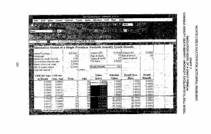
I have implemented this model on Microsoft Excel using Crystal Ball, once again. Chart 3 shows a screen shot of the model. You can see that the death benefit is boxed here in the middle of the screen. You can see that the initial parameters are in columns A through C, and the model results, including the death benefit, are in columns E, F, G, and H.

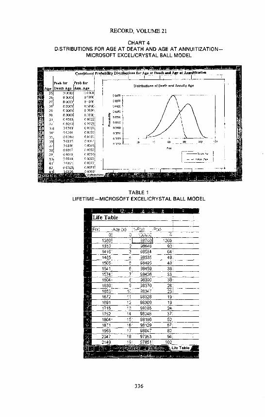
Chart 4 shows the probability distributions for age at death and age at annuitization. Using a spreadsheet, we can plot these distributions as shown. Interestingly, the distribution for age at death, which was taken from an actuarial text, has a little blip at age 80. Maybe that is a typo or some other error.

Table 1 illustrates the life table used in the model. It 's not particularly fancy. I will note that to sample from a discrete distribution, we need the cumulative distribution function rather than the individual probabilities. In fact, this model uses the conditional distribution of age at death, given the person reached the age they were when the annuity was pur- chased. So, part of the computations involved computing this conditional distribution; as well as the corresponding conditional distribution for age at annuitization.

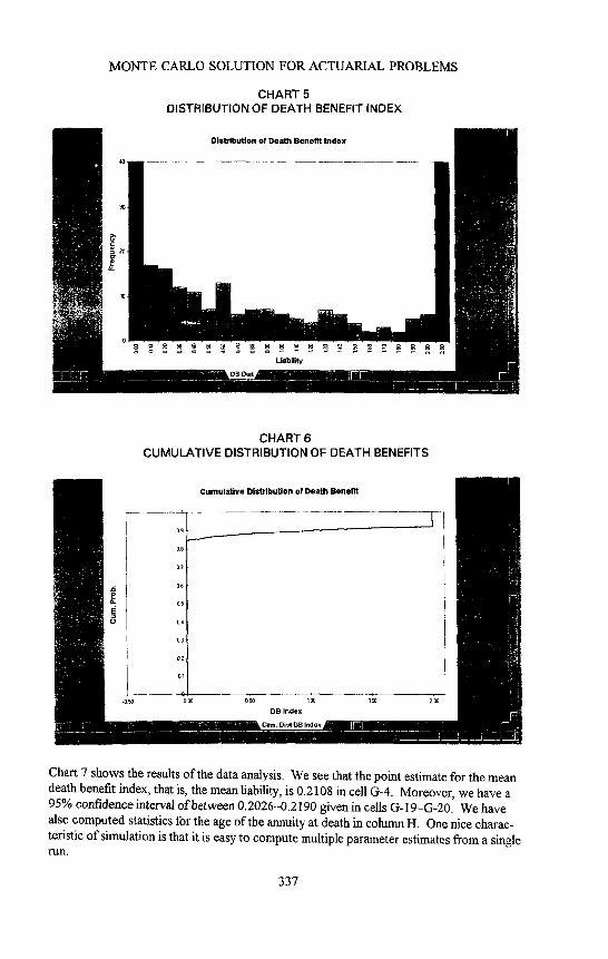
Chart 5 is the histogram for the death benefit index. Recall that we used the term "index" because the death benefit was based upon $1 invested. Note that this distribution has a very large spike at 0 and at 2. Many of the annuities were cashed in before the owner died, and for those where the owner died, many reached the maximum liability of 2.

This characteristic of the distribution is even more apparent here on the cumulative distribution of death benefit as shown in Chart 6. We see that approximately 85% of the replications resulted in no liability. About 10% resulted in the maximum liability of two, and the rest were distributed between these two limits. This is a pretty weird distribution, and I doubt seriously if it could have been found with strictly mathematical means.

334

Ariel

Fi le ~ l t V i e w I n s e r t F o r m a t ]~ools D a t a W i n d o w Cel l Run J: lelp

EI~ =E13"(1+ CBNoFmaI($C$7,$CS8))

S i n le P r e m i u m V a r i a b l e A m i u i t y D e a t h ] B e n e f i t . I [ S i m u l a t i o n M o d e l o f a g . . . . . . . . . . . . . . . . . . . . . . . . . . . . . . . .

; . . . . . . . . . [ t . . . . . . $25 000 iUn form RV 0 4516 Uni form RV 1 0.0066 /

Initial Purchase - ' -36 . . . . . f~,go-a[ death . . . . . . . . . ~ " ~ , g e - E a n n u i t . " . . . . . . . . . . . . . . . 32 [ . . . . . . . . . . . Initial age ~ . . . . . . . " i ;Maximum death benef i t 2.00 Years at death 47 Years at annu~t. 21 [

2.0000 Guaranteed interest rate 6 00% DI3 Index j i ,Mean return per year 9.00%~ t , SD of year ly return 13.00% [DeathBenef t t $0 . . . . . 1

Ratchet interval 51Years [ ]

D e a t h B e n . D e a t h i C D F fo r A g e - C D F f o r , V a l u e R a t c h e t a t D e a t h A m L Age., . . . . . i~ldex V a l u e ...... i ~oo r [ Be~tefi t ] ],

0.0000 o.o0ooi 0 0 0 1 3 0.0022i 0 0 0 2 6 0 .0047[ 0.0040 0.00751 0 0 0 5 3 0 .0107[

_ o . o ~ o . o ~ 0.5838 0 9996 0.6152 0 99991 0 6 4 7 1 1 0000 i 0 6 7 9 0 1 0 0 0 0

Deolh B~'enetit Model t

Yem" i ABe 0 30t

11 31 2[ 32 3 3~,1 4 t 34;

_ _ 5! 3~ 52 82

84 551 85

1.0000

..... 6q:(]25~sj 80.7604

1.oooo 1.oooo i o.oooo .......... , ............ i i iTO iiO~oo001 1.0000

~i00o6 , . . . . 1 . 3 5 4 1 o . o o o o

1.oooo; .................... i 98621 65666 . . . . i 1160651 ............. 119342[ ......... 010006} i i . 6 6 8 4 . . . . . . . . . . . . . . . .

o.o2,,= 1 ,,4o I o.oooo 6.dSg~ l ................ g-b;65-Sg . . . . . 516~d6

. . . . . . . . . . l . . . . . . . :io 8t o.o6oo ............... 8o.76o4 0 oo0o

<

) , 8B I - ra

Z Z C - I .4

- r

m Z

O (/) o

- I ) , f -

) , r r - E O O m t -

t~

- I : ~ c o ¢t}

g

,-]

O

©

©

,-]

wtl

r.I)

RECORD, VOLUME 21

CHART 4 DISTRIBUTIONS FOR AGE A T DEATH AND AGE AT A N N U I T I Z A T I O N - -

MICROSOFT EXCEL/CRYSTAL BALL MODEL

331 341

Cond tlonal Probability Distributions lot" Age at Death and Age at Annultlzatlon ! . I ] '

Prob. for. I, Distributions of Death and Annuity Age

O 0000 o oo0o 0 0000! o 00o61 o ooool 00013] OOQI3! 0 0013" O 0014 o o0i4 O OOI5 i Sums ooo 7 00018] o~ 0 O02i 1 oo053[

000001 0 0000[ 0 0000i 0 00001 00000~ 00000[ 0 0022! 0 00251 0 0028[ o 0032[ O 00361 0 0041 0 0o40! 0 0052[ 0 0058 i 0 0005 i 0 0072: 000811

0 o,Loo . . . . . . . . . . . . . . . . . . . . .

o 83oo ~,

o o2r~

00150 •

O0180 -

00050

ocf£n4- . . . . 4 ~ - . . . . ~ . . . . . . ~ - ; --, "~tl dO 60 80 tot} ~)

0 r;~sO . . . . . . . . . . . . . . . . . . . . . .

I_-_[- ;u .....

TABLE 1 L IFETIME- -MICROSOFT EXCEL/CRYSTAL BALL MODEL

Life Table i

[ 1-F(X) P /× ! I

Oi 0 sOOOOO 0 1260

13521 2 98648 92! 1416 3 98584 64! 1465 4: 98535 49; 1505: 5 98495 401 1541 6: 98459 36i 1574: 7! 98426 33! 1604- 8! 98396 30! 16301 9 98370 26t 1653: 10: 98347 23! 1672 11 98328 19: 16911 !2 98309 19 ! 1715 13 98285 24 1752! 14 98248 37; 1804! 15: 98196 521 1871 16: 98129 67i 1 ~ ? 17 98047 82~

18 97953 941 19: 97851i 102j

3 3 6


CHART 5 DISTRIBUTION OF DEATH BENEFIT INDEX

CHART 6 CUMULATIVE DISTRIBUTION OF DEATH BENEFITS

. . . . o~

09

07

Q6

05

04

03

02

01

-o'5o °oo

Cumulative Distribution of Death Benefit

DB Index

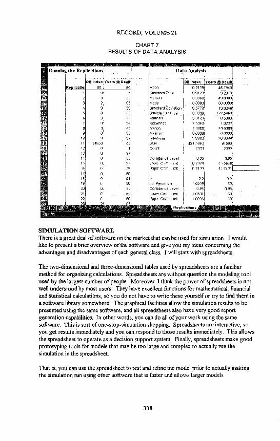
Chart 7 shows the results of the data analysis. We see that the point estimate for the mean death benefit index, that is, the mean liability, is 0.2108 in cell G-4. Moreover, we have a 95% confidence interval of between 0.2026-0.2190 given in cells G- 19-G-20. We have also computed statistics for the age of the annuity at death in column H. One nice characteristic of simulation is that it is easy to compute multiple parameter estimates from a single r u n .

337

RECORD, VOLUME 21

CHART 7 RESULTS OF DATA ANALYSIS

ieations! ] t Data Analysi~ ]

DB ndexlYears~Death DBIndex Years(~Death! ""

$0 6Oi .Mean [3 5 ~Stand~rd Errol 0 26 Median 2, 55 Mode 0 581 Standard Deviation 0 60 Samole Vanance 0 36 Kurtosls 0' 56 Ske'~neee r 45 Range 0 36 MIR[FnLIm

B 37 M~y,~rnlJm

24853 48 ~um 0 l CoHnt

27 O 30 30rlNdence Leve O 38 Lower Conf Limit 0 2E Uol2er Conf Limit

0.2108 457540 0 0 t29 8 2879 0.0OOO 49 00O0 O 0800[ 60 0000 gf i778 ~3 3246 0.3338 177 5463 5 0123 O 5883 2 5962 ~ 8232

2 00O0 60 0000 O.8OO0 0 nooo

g80~ ~O 0000 421 5862 91508

20n0 ?~On

0 35 3.35 02826 ,I5 5646 8 2190 43 $4341

17 0 613

18[ 0' 83[ ~ 09 09 19 0 50 Fth Percentile 1 0559 60 20 0 68 Confidence Level 0 95 0 95

/ 211 0 501 LoWer Conr Unlit 10501 60 ~ ! y ?pper_ Oo~f~,Urnit 105861 60

Replications

SIMULATION SOFTWARE There is a great deal of software on the market that can be used for simulation. I would like to present a brief overview of the sot~ware and give you my ideas concerning the advantages and disadvantages of each general class. I will start with spreadsheets.

The two-dimensional and three-dimensional tables used by spreadsheets are a familiar method for organizing calculations. Spreadsheets are without question the modeling tool used by the largest number of people. Moreover, I think the power of spreadsheets is not well understood by most users. They have excellent functions for mathematical, financial and statistical calculations, so you do not have to write these yourself or try to find them in a software library somewhere. The graphical facilities allow the simulation results to be presented using the same software, and all spreadsheets also have very good report generation capabilities. In other words, you can do all of your work using the same software. This is sort of one-stop-simulation shopping. Spreadsheets are interactive, so you get results immediately and you can respond to those results immediately. This allows the spreadsheet to operate as a decision support system. Finally, spreadsheets make good prototyping tools for models that may be too large and complex to actually run the simulation in the spreadsheet.

That is, you can use the spreadsheet to test and refine the model prior to actually making the simulation run using other software that is faster and allows larger models.

338


While I strongly recommend the use of spreadsheets, I want to caution that they are not simulation nirvana. First, the built-in random number generators are usually 16-bit generators and not recommended. Normally, these random number generators are implemented in a function such as RAND 0 or @RAND. They are fine for prototyping, but for serious simulation work, they should be avoided. Later we will discuss why these random number generators are inadequate.

Fortunately, there are add-in packages for simulation that provide much better random number generators as well as specialized functions for sampling from a large number of distributions. I will have more to say about this a little later. A second problem with spreadsheets is that recalculation can be slow. Simulations must be replicated in order to get the data to compute confidence intervals. Replications normally are produced by recalculating the spreadsheet. If the model is complex, the recalculations can be quite time consuming compared to other software options. Fortunately, spreadsheets are being programmed to recalculate faster, and computers are faster. So, for moderate-sized models, this is not a major problem. The final problem I see with spreadsheets is that models will not be portable to other computers. The model will be portable only if the same spreadsheet is running on the other computer, or if another spreadsheet is running that can read the original model's file format. Contrast this to writing the simulation program in a general language such as Pascal or APL. Then, the model can be run on any computer that has the appropriate compiler or interpreter. This can be important if you want to write and test a model on a desktop computer, then run it on a large mainframe computer.

There are a couple of very nice simulation add-in packages that are available for Lotus 123 and Microsoft Excel. One of these is Crystal Ball, which I used to help with the simulation examples we just looked at. Another is @RISK, which you have probably seen advertized. These packages provide good random number generators so you do not have to use the built-in generators. They also provide convenient functions for generating random variate from a large number of distributions. Facilities for doing the replications, storing the data and graphing the results are included too, Actually, the main reason I advocate the use of these packages is to use the random number and random variate functions included in them. I find it easier to use the built-in capabilities of the spreadsheet to do the other activities in a simulation.

Of course, spreadsheets are not the only choice in simulation software. There are many other possibilities, from general purpose languages to very specialized simulation software. Let's look at general purpose languages such as FORTRAN, Pascal, or C. If they are to be used for simulation analysis, these languages must be supplemented with a library of routines for random number generation and for generating variate from various distributions. There are several providers of these routines, for example, IMSL and NAG. General purpose languages have the advantages that they are familiar and the programs run quite fast. Most people have studied one or more of these languages, so the learning curve is not too steep. The simulation programs--at least in source code form--are also portable to any other computer that has the same language compiler. These languages are so ubiquitous that they are available for virtually all computers, from the smallest micro- computers to the largest multiprocessor mainframes. General purpose languages have the disadvantage that they are not interactive. Programs must be written using a text editor,

339

RECORD, VOLUME 21

then compiled, then run, then revised, and so on. The simulation program development process is extended because of this relatively unwieldy sequence.

APL is also a possible simulation language. I would put this language in a class by itself because it is an interactive language that is very high-level and quite well-suited to mathematical calculations. It is also quite fast, and one advantage over general purpose languages is that it is interactive, so programs can be written, tested and revised more quickly. If you use APL, you should check out the random number generator carefully, as you should with all simulation software. One disadvantage of APL is that it is not generally available, so the programs are not portable from one computer to another. So, if you develop a simulation on one computer, you are usually stuck with running it on the same computer.

A number of general purpose simulation languages are available for all types of computers, from desktop systems to mainframes. Some of the better known languages are SIMSCRIPT 11.5, SIMAN, and GPSS/H. There are many others, so don't take this short list to be representative. These languages have, for the most part, all of the capabilities e r a general purpose programming language, plus they have simulation capabilities (random number generators, routines for sampling from various distributions and perhaps data analysis routines) built-in. An advantage of general purpose simulation languages is that the random number generators and routines for sampling various distributions are well-tested and efficiently implemented. You can be sure that the random number generator is state-of-the-art. Unfortunately, most simulation languages were designed with discrete event simulation in mind. Discrete-event simulation is a modeling methodology that is useful to represent many systems involving queuing and service. There may be a place for discrete-event simulation in actuarial science and financial modeling, but that is a topic for another session, and I am assuming that this is not the modeling methodology being used. As a result, simulation languages are not natural to use in financial modeling.

A final choice is mathematical software such as Mathematica, MathCAD, Maple, Matlab, GAUSS, and so on. Over the past few years, quite a number of interactive software packages of this sort have been introduced. These are available for all personal computers and many high-performance workstations and mainframes. They have great computational facilities and excellent graphical capabilities, so they allow the computations to be implemented and the results to be graphed interactively in the same software. On the negative side, however, the random number generators may be suspect. I have had little luck finding out exactly what algorithms were used in the random number generators when I have asked. The packages also do not have built-in routines for sampling from various distributions. Basically, these packages were designed for numerically intensive computing, but not simulation. The means of implementing calculations is relatively high-level, and many of these packages do not have an algorithmic language. Often this is not needed, but in many simulation models it is very useful if not absolutely necessary. If models can be success-fully implemented, many of these packages have good interfaces with general purpose languages such as FORTRAN or C, so the calculations can be easily translated to these languages for further sampling and study.

PSEUDO RANDOM NUMBER GENERATORS (RNGs) I will use the term random number to refer to an observation that is sampled from the uniform distribution between zero and one. The term is also used to refer to an integer

340


observation that is uniformly distributed between either zero or one and some upper limit. In practice the former variate is computed from the latter by dividing by the upper limit, so the dual use of this term is not as ambiguous as you might think at first. A random variate refers to an observation sampled from a specified distribution, such as the normal distribution, or the binomial distribution. All sampling on the computer is performed using random variate generation routines, which are simply subroutines or functions that retum a value that behaves as if it were sampled from the specified distribution. Actually, since these routines are deterministic in nature, they are often called pseudorandom number generators. I will just call them random number generators, however. I will not specifi- cally talk about random variate generation routines because they are built into most simulation software, so to use them you just call the appropriate routine and pass the appropriate parameters to it. There is well-established literature on random variate generation methods also, in case you want to write your own routines from scratch. See the textbooks in the list of references in the handout for more information.

On the other hand, I want to say several things about random number generation routines, or random number generators, for short. Every random variate generation routine operates by first generating one or more random numbers, then performing some transfor- mation on them to produce the random variate. We want the random variate to not only behave as if they were sampled from the correct distribution, but also to show the property of being mutually independent. Since the random numbers are the basic input to the random variate generator, the quality of the random variate is controlled by the quality of the random numbers.

This reminds me of an experience I had several years ago. I had a consulting job that involved a large hospital. Medicare had audited the hospital and selected a random sample of a little over 100 claims from all of the Medicare claims filed in the previous year. On the basis of the audit of these claims, Medicare declared that the hospital owed them a refund of $10 million! I was asked to examine the sampling methodology and see if the program that randomly sampled the claims might have selected a biased sample. Now, this program used a random number generator along with an algorithm to determine which of the claims in the population would be selected for the sample. So, my first action was to ask the accounting firm (which was one of the then Big Eight) that did the audit what algorithm was used in the random number generator. My requests were met initially with si- lence~the accountants did not know what random number generator was used. Later, I was told that the algorithm was proprietary. Well, that was enough information for me to claim that the sample could not be shown to be legitimate, and therefore that the refund request should not be honored. It is incumbent upon the person doing the sampling---or simulation--to demonstrate that the random numbers used truly behave like uniformly distributed, mutually independent random numbers. This is simply a matter of professionalism. I will tell you how the matter was resolved in a few minutes when I talk about output data analysis.

Before I talk about good and bad random number generators, I want to show you a couple of random number generators so you will see what I am talking about when I use such terms as cycle length and seed. A linear congruential generator has the form following: Z~.l=(+aZj+b) (mod m) Each random number is computed by transforming the previous random number. Thus, we can talk about a sequence or stream of random numbers. The first number in the stream is called the seed (Zo). Of course, we can think of any random

341

RECORD, VOLUME 21

number in the stream as being the seed for the remaining random numbers. Notice also that this random number generator has three parameters: a, b, and m. The values of these parameters determine the properties of the generator, so we want to use values that produce a sequence of random numbers with good properties. (Ui = Z/m are the pseudo random numbers that are uniformly distributed between zero and one.)

Most random number generators used in simulation software packages today are multipli- entire linear congruential generators, where b=0. These are used because they produce the values relatively fast, and they have been found (with the right parameters) to produce a high-quality sequence of random numbers. If m=216, this is called a 16-bit random number generator: Zi+~=aZ~ (rood 216). If m=232, it is called a 32-bit random number generator: Z~+I = a ~ (mod 232). In this case, there is only one parameter, a, that determines the quality of the random numbers produced.

A random number generator that is used in many simulation packages is the 31-bit prime- modulus multiplicative congruentiat generator. The formula used to compute each random number from the previous is: Z~+l=aZ~ (mod m). In this case, the value ofm is the largest prime number less than 23~, which is 231-1. This generator requires a little more computational effort than the 32-bit generator, but studies have shown that it has excellent properties, and this is the reason why it is used in so many simulation software packages. The Excel add-in, Crystal Ball, that I have been using, uses this generator. Fishman and Moore evaluated every possible multiplier, a, for this generator and published a table giving the best multipliers. The paper, which is in the list of references, can be used as documentation of the quality of the generator if you are using this generator.

What do I mean by quality of the random numbers? This is a multifaceted question. As I indicated earlier, we want the numbers to behave as if they were sampled independently from a uniform distribution. But, we also note, because each number is the seed for the next number and that all numbers must be between zero and m - 1, that at some point the starting number will be produced again, and from this point on the sequence will begin repeating. The number of random numbers that can be produced before the sequence repeats is called the cycle length of the generator. Obviously, we want the generator we use to have the longest possible cycle length.

For multiplicative congruential generators, when you consider pairs of random numbers and plot them on the plane, you will find that they actually fall entirely on a series of diagonal parallel lines. So, they are not truly independent. If the lines are close enough together, however, they will act very much like independent pairs ofvariate. Similarly, if triplets are plotted in three-dimensional space, they will fall on parallel planes, and i fn tuples are plotted in n-dimensional space, they will fall on n one-dimensional hyperplanes. We want the closest of these hyperplanes to be as close as possible. These are what I call good higher-dimensional, or geometric, properties. Of course, we want the random number generator to be as fast as possible and to use a reasonable amount of computer memory. This consideration about memory usage was important a decade ago when memory was expensive. Now, it is much tess of a concern.

So, how do we know whether a given random number generator is good or not? The short answer is that we must rely upon experts to test the random number generator and certify the behavior. These tests involve statistical tests as well as analysis of the geometric

342


properties. A number of generators have been tested. L.R. Moore lists random number generators that are known to have good properties. In addition, A.M. Law and W.D Kelton describe a couple of random number generators that are known to have poor properties, the most notorious of these being RANDU, which was part of IBM's Scientific Subroutine Package for a long time. As I mentioned earlier, Crystal Ball and @RISK provide good random number generators if you are using a spreadsheet to develop your simulation.

I would recommend that you not ever use a 16-bit random number generator for anything but prototyping a simulation. The longest possible cycle for these generators is 65,536, and most of them have much shorter cycles--shorter than 16,384. You don't have to generate many random numbers before you have reached this number and the cycle begins repeating. On the other hand, a good 31-bit random number generator can have a cycle length of approximately two billion. This is plenty of random numbers for virtually any simulation experiment.

If you use a certified and accepted random number generator, you can be reasonably sure that your results are correct, and you are not subject to criticism that you used substandard methodology. On the other hand, if you use a random number generator that does not have good statistical and geometric properties, you cannot be sure whether the random number generator introduced error into the model. Maybe it did and maybe it did not. You just don't know.

ANALYSIS OF INPUT DATA Any stochastic simulation will have at least one, and usually more, distributions from which observations are to be sampled. Before the model can be considered a valid representation of the intended process, data from the distributions must be collected and an appropriate theoretical distribution must be fit to the data. For example, in the model presented earlier concerning life insurance for a single-premium variable annuity with ratchet, data must be collected on the age at annuitization, given the age at purchase, and fit to a gamma distribution, or a lognormal distribution, or some other appropriate distribution. Statistical procedures are well established for estimating parameters for most common distributions using the method of maximum likelihood and other methods. The Kolmogorov-Smimov test is available for testing for goodness of fit to the fitted distribution. I will not spend time discussing these procedures today because they are available in standard statistical texts. Instead, I want to just make a few comments about distribution fitting.

One option that I have seen used too frequently is to just sample from the empirical distribution. That is, no parameter estimation or distribution fitting is done at all. In general, this is a bad idea. There are a couple of reasons why I believe it should not be done. First, the data are just a sample from the parent population, so your simulation would be just resampling a sample. Another sample from the parent population would produce another empirical distribution, and sampling from that distribution could result in conclusions entirely different from those obtained from the first empirical distribution. In short, your simulation results would reflect the specific properties of the sample, not the parent population. Second, these effects can be especially strong in the tails of the distribution. Since observations in the extreme tails of the distribution can be very rare in practice, they will often not be included in the empirical distribution. However, in many models the more extreme an observation, the more extreme its effects on the model, and to

343

RECORD, VOLUME 21

get an accurate picture of the model performance, you have to simulate the model long enough to get some of the extreme observations. If they are not present in the empirical distribution, you will never get any of them.

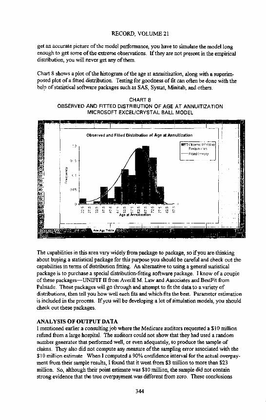
Chart 8 shows a plot of the histogram of the age at annuitization, along with a superim- posed plot of a fitted distribution. Testing for goodness of fit can often be done with the help of statistical software packages such as SAS, Systat, Minitab, and others.

CHART 8 OBSERVED AND FITTED DISTRIBUTION OF AGE AT ANNUITIZATION

MICROSOFT EXCEL/CRYSTAL BALL MODEL

I L . . . . . . . . . . . . . . 1 . . . . . . . . . . . . . . . . . . . I /

Observed and FRied Distribution of Age at AnnuRization i

:i ii Ill ~ ~ ~ ~ ~- ~ ~ ~ ~ ~ ~ ~ ~ ~ :

Age at Annultlzatlon i I

N I__ . . . . . . . . . . __A ! 1!1 Ann Age Tobla

The capabilities in this area vary widely from package to package, so if you are thinking about buying a statistical package for this purpose you should be careful and check out the capabilities in terms of distribution fitting. An alternative to using a general statistical package is to purchase a special distribution-fitting software package. I know of a couple of these packages--UNIFIT II from Averill M. Law and Associates and BestFit from Palisade. These packages will go through and attempt to fit the data to a variety of distributions, then tell you how well each fits and which fits the best. Parameter estimation is included in the process. If you will be devdoping a lot of simulation models, you should check out these packages.

ANALYSIS OF OUTPUT DATA I mentioned earlier a consulting job where the Medicare auditors requested a $10 million refund from a large hospital. The auditors could not show that they had used a random number generator that performed well, or even adequately, to produce the sample of claims. They also did not compute any measure of the sampling error associated with the $10 million estimate. When I computed a 90% confidence interval for the actual overpayment from their sample results, I found that it went from $3 million to more than $23 million. So, although their point estimate was $10 million, the sample did not contain strong evidence that the true overpayment was different from zero. These conclusions

344


were obtained without even looking at the auditing procedure or disputing the conclusions on any specific claims. The result was that the hospital did not have to pay back the $10 million. Unfortunately, I was not paid a commission on the savings. I would have been very happy with just 10%T

After any simulation is run and the output data produced, the final step is to perform a statistical analysis to estimate whatever parameter you are seeking to know about the system. In the example mentioned about life insurance for a single-premium variable annuity with ratchet, we wanted to know the expected value of the liability. So, our simulation produces data on the liability and we have to use it to compute point estimates and confidence intervals for the expected value. Interestingly, in preparing this session, I looked in a number of actuarial publications for examples of simulations of actuarial problems. Of the eight to ten articles I found, none of them included multiple replications with a statistical analysis of the output data!

You might ask why we should subject the output data to statistical analysis. Well, first and foremost, a simulation is a sampling experiment, so any data produced is subject to sampling variation. If we rerun the experiment, using independent random numbers, we will get a different set of data. So, we must use some method to compute the statistical accuracy of our point estimates. If you just run the simulation once and accept the output as the true parameter value, you are doing something analogous to collecting a single observation on a claim and using its value to represent the mean of all claims. Without a measure of accuracy, which is a confidence interval, you simply do not know how accurate your estimate is. If your estimate is not accurate enough, you need a measure of variation to compute how many observations, or replications, you need to generate in order to achieve an acceptable level of accuracy.

It is important to subject your output data to statistical analysis. The next question is: What types of statistical analysis are appropriate for simulation output? There are two basic types of output data: Independent observations fi'om multiple independent replications, or scenarios, and time series observations from one or more independent replications. The liability at time of death or the value of the account at time of death in the last model, are examples of the first type of output data. The simulation is run for multiple independent replications. In each replication, the replication ends when the annuitant dies and the liability can be computed, producing a single observation. On the other hand, if we consider the value of the account each year, over a period of years, or the insurer's liability each year, we have time series data. The methods used for statistical analysis differ in these two types of data. I don't have time here to talk about time series analysis. This is a specialized topic and will have to be the subject of a future session. Fortunately, if the simulation run consists of independent replications, the usual statistical methods which are described in any introductory statistics text can be used to compute confidence intervals for the parameters we're interested in. Let's look at these using the example we've been considering. A confidence interval for the mean liability at the time of death is computed using the usual formula for a confidence interval for the population mean. When we apply it to the data from the simulation, we get the range 0.1583-0.2273 as the following shows:

Y ±Z~2s ~ 0.1928 4- 1.96(0.0176) = 0.1583 - 0.2273

345

RECORD, VOLUME 21

This is a pretty wide range. If we compute a confidence interval for the standard deviation of liability at the time of death, it ranges from 0.5345 to 0.5836 as the following shows:

(n-1)s2 < VAR(Y) < (n-1)s2

X~2

A confidence interval for the 90th percentile of liability at the time of death is from 0.4272 to I. 1120 as the following shows:

< , . 9 0 < r(,,) (r(s9o), Y(9,o9 = (0.4272, 1.1120)

This latter confidence interval is a nonparametric interval, computed using the order statistics from the sample. You may need to consult a more advanced text on statistics to find out how to compute this interval.

There are a large number of statistical software packages: SYSTAT, SPSS, MINITAB, and others, available today for use in analyzing data. These can, of course, be used to analyze data produced by simulations. In general, I would recommend that you have your simulation to write its output data on a file and use a statistical package to do the parameter estimation and confidence interval computations. The primary advantage of this approach is that there is less room for error because the computation routines in the established statistical packages are well tested. Of course, use of existing software saves time and effort. Finally, if you put your data on a file, you will not have to rerun the simulation if you decide to compute another parameter from the data or do some other statistical analysis with the data. On the other hand, sometimes you want to apply computations that do not exist in statistical software, or you want to set up the simulation so that it can be used routinely by actuaries. In this case, you will want to program the statistical analysis along with the simulation.

Finally, it is often a good idea to plot the output data and subject it to many of the same types of statistical analyses that you would apply to data coming from the real world. A plot of the histogram or frequency polygon of the data will show quickly the shape of the distribution and whether it is skewed or not. If multiple scenarios are compared, a plot of their means and confidence intervals will show quickly how they compare. Most of the statistical packages have excellent plotting capabilities (as do spreadsheets) to accomplish this.

MODEL VERIFICATION AND VALIDATION All simulation models should be verified and validated before being used for decision making. This seems rather obvious to me. Indeed, all models should be verified and validated, not just simulation models. What do I mean by verification and validation? Remember that we first create a model of the system we are analyzing. A model is not a recreation of the system, but an abstract and simplified representation that includes the most important features of the system. Verification is the process of assuring that the model implemented is the model intended. It is basically a debugging activity. You want to assure that the simulation program behaves like the model you intend to implement. For

346


simulation programs this can be a formidable task because the simulation produces output that is random, so you can't always predict exactly what will be produced.

I have a few suggestions concerning verification of simulation models. First, build the model without the random number generators initially. Instead, put specific values in the place of random variate and check the computations to assure that all formulas are correct. You might use values on input files instead of random variate as the source of the variate, then read them into the program at the point where you would normally call the random variate routine. This gives you the opportunity to compute by hand exactly what should be computed and compare it with the values that are computed by the program. Second, examine the output for reasonableness. You should frequently have a good feel for the distributions of the output data. Often you will know if the output data has a highly skewed distribution, or if it has a mass at a particular point. Third, consider extreme or unusual cases. Try to create input that should produce these circumstances and see if the program actually does produce them. For example, ifa particular policy has a provision for coverage that would normally only happen once per 10,000 policies, produce some input to make it happen to assure that the logic of the program handles the events cor- rectly. Four, ask other colleagues who are familiar with the project to check the model. After you have looked at a model long enough, you start seeing what you expect to see. It is ot~en helpful to get another point of view, even if it is from a person somewhat less intimately acquainted with the project than you. Finally, you can't check enough. Double check. Triple check. Then, cheek again. Most models are fairly complex, so it is easy to miss an important detail. And remember, the devil is in the details!

Now, validation, on the other hand, is the process of assuring that the model implemented adequately describes the real process being modeled. Validation makes sure the model is useful for decision making. Note that you verify a simulation program, but you validate a model. In order to validate a model, you have to have data or other information from the real system. Basically, in validating a model, you want to compare the distribution of the data output by the model, when the model parameters are set to reflect those of the existing system with the corresponding data from the real system, and assure yourself that the two sets of data come from the same parent population. There are several methods to compare these distributions. You could use the two-sample Kolmogorov-Smirnov test for goodness of fit, or you could just do hypothesis tests for equality of the means and variances of the two distributions. If another characteristic of the distributions is important, you could do an hypothesis test for equality of this characteristic. An interesting alternative that has been promoted involves an actual manager of the real system. Have the model to produce a report exactly like a report the manager receives from the real system. Present her with reports from both the model and the real system, and see if she can tell which is the real report. If she can't, chances are good that the model is valid, at least as far as the information on the report goes.

METHODS FOR IMPROVING THE EFFICIENCY OF SIMULATIONS I had hoped to have some time to talk about efficiency improvement techniques, or variance reduction techniques, as they are often called. Briefly, this is a collection of techniques that allow you to compute more precise estimates of the parameters you are interested in without having to greatly increase the sample size or computing effort. The nice thing about simulation is that you have total control of the experiment. You can therefore do such things as induce correlation between output processes, and this

347

RECORD, VOLUME 21

correlation can give you more precise estimates of the mean of the process. These techniques can be applied in certain specific circumstances, and they do not always guarantee a variance reduction. Indeed, they can inflate the variance!

Remember that your simulation results are only as good as your (1) model, (2) data analysis, and (3) ability to understand the simulation procedure and explain it to others who will be using the simulation results. The simulation process is like a chain with these three links. It is only as strong as the weakest link, and it needs all three links to operate properly.

Your first objective is to have a correct, valid model. Every model is suspect until it has been validated, and yours is no exception.

You should use at least a 31-bit random number generator. No 16-bit random number generator will have the qualities you want for serious simulation. As I indicated earlier, it is your responsibility to make sure the random number generator that is the basis for all random variate generation computations in your simulation has been tested thoroughly and found to satisfy the qualities of a good random number generator.

Your data analysis should include error estimates as well as point estimates of the quanti- ties you are seeking. Error estimates are usually computed in the form of confidence intervals for the mean, but they can also be given as the standard deviation of the parameter estimator.

Finally, some efficiency improvement, or variance reduction techniques, are available to improve the precision of parameter estimates. These techniques can often provide substan- tial improvements in the precision, but they do not come with guarantees.

348


SELECTED BIBLIOGRAPHY ON MONTE CARLO METHODS

Bratley, P., Fox, B. L., and Schrage, L.E., A Guide to Simulation, 2nd ed., Springer-Verlag: Berlin, 1987.

2. Fishman, G. S., Principles of Discrete Event Simulation. John Wiley: New York, 1978.

3. Fishman, G. S. and Moore, L. R., "An Exhaustive Analysis of Multiplicative Congruential Random Number Generators with Modulus ," SIAMJ. Sci. Star. Comput., 7, 24-45, 1986.

4. Hammersley, J. M., and Handscomb, D. C., Monte Carlo Methods. Methuen: London, 1964.

Law, A. M. and Kelton, W. D., Simulation Modeling and Analysis, 2nd ed., McGraw-Hill: New York, 1991.

Lewis, P. A. W. and Orav, E. J., Simulation Methodology for Statisticians, Operations Analysts, and Engineers. vol. 1, Wadsworth: Pacific Grove, CA., 1989.

7. Morgan, B. J.T. The Elements of Simulation. Chapman& Hall: London, 1984.

Rubinstein, R. Y. Simulation and the Monte Carlo Method. John Wiley: New York, 1981.

349

monte carlo solution for actuarial problems - member · monte carlo solution for actuarial problems...

Documents