monthly holdings data superior mutual funds edwin...
TRANSCRIPT

Monthly Holdings Data and the Selection of
Superior Mutual Funds+
Edwin J. Elton* ([email protected])
Martin J. Gruber*
Christopher R. Blake** ([email protected])
July 2, 2007
* Nomura Professor of Finance, Stern School of Business, NYU ** Joseph Keating, S.J., Distinguished Professor, Fordham University + We would like to thank Ken French for supplying us with weekly data on his factors.

Monthly Holdings Data and the Selection of Superior Mutual Funds
Abstract
This paper examines the use of holdings data to estimate mutual fund
alphas and betas and to select funds that outperform index funds. The paper presents
evidence of the stability of betas and the consistency of alphas across estimation
techniques. It also presents evidence that using alphas estimated from mutual fund
holdings greatly improves an investor’s ability to predict future alphas and to select funds
that outperform index funds. Finally, the paper has major implications both for the SEC’s
recent ruling on the required frequency of holdings reporting and for the information plan
sponsors should collect from portfolio managers.
JEL Classification G11, G12
Keywords: mutual funds, portfolios, composition, performance prediction
There have been a number of studies that use mutual fund return data to compute
performance measures and which show that funds that rank high on these performance
measures perform well in the future.1 In this paper we examine whether monthly holdings
period data can be used to identify funds that will outperform other mutual funds,
outperform passive portfolios, and outperform mutual funds selected by the most
commonly used ranking devices. Two measures that we will use to rank funds are the
alpha from the Fama and French three-factor model and the alpha from the four-factor
Carhart model. Why might holdings data produce better estimates of betas and alphas
than simply using the traditional method of obtaining betas and alphas by regressing past
mutual fund returns on a set of indexes? Portfolio betas (mutual fund betas) are a
weighted average of security betas. Thus we can compute the mutual fund beta from
individual security betas using holdings data at a point in time. This is the beta on the
mutual fund at that point in time. A big advantage of this technique compared to a time
series regression of fund returns on indexes is that the fund beta will not be distorted by
changes in the beta on the portfolio caused by changes in the composition of the portfolio
over time.
This paper contributes to the literature in three ways by examining the following
questions:
(1) Does the use of holdings data provide a better way to estimate sensitivities
(betas) and alphas than simply using a time series regression on a fund’s past return?
(2) Does the use of holdings data lead to a better selection of funds?
1 See, for example, Elton, Gruber and Blake (1996), Gruber (1996), Zheng (1999), Bollen and Busse (2001), and Mamayski, Speigel and Zheng (2005).
1

(3) What is the effect of different frequencies of reporting holdings data, and
how frequent should holdings data be reported to get most of the benefit?
Our primary results are that estimating alphas using betas computed from
holdings data allows us to rank funds on alpha such that 1) the top two deciles formed
from these rankings outperform index funds in the next period, 2) the performance in the
next period of the deciles is almost perfectly correlated with the prior ranking, and 3) the
performance in the top decile is considerably higher than that found by others in past
research. These results hold whether we evaluate performance in the ex-post period using
alphas estimated from holdings or estimated from a standard time series regression of
fund returns on indexes. In addition, we show that ranking funds on the basis of alpha
computed using monthly holdings data leads to better ex-post alphas than ranking on
quarterly holdings and that both rankings are substantially better than ranking based on a
time series regression on fund returns.2 Demonstrating that monthly holdings lead to a
better ranking of funds than quarterly holdings has important implications for investor
behavior. The availability of monthly holdings data has been growing and is now
available for about 18% of all domestic mutual funds. Our results indicate that when
available, such information should be used and that public policy should encourage the
move towards monthly reporting of holdings. In addition, administrators of institutions
such as pension funds (plan sponsors) who should be able to obtain monthly holdings
data from the managers who run these funds should do so.
There has been a lot of discussion about how often funds should be required to
report holdings data. The law has changed, and probably will change again. In the 1970’s
2 Quarterly reporting misses about 18% of the mutual fund trades (see Elton, Gruber, Krasny and Ozelge (2006)).
2

and 1980’s, funds were required to report holdings on a quarterly basis. Subsequently,
funds were only required to report semi-annually, but recently the requirements were
changed back to quarterly. The decision on how often funds should be required to report
requires an analysis of the costs and benefits of more frequent reporting.3 This article
contributes to this debate by showing one benefit to investors of having holdings data at
more frequent intervals.
The paper is divided into four sections. In the first section we discuss our sample
of monthly holdings data. In the second section we discuss and present evidence on
whether using holdings data can improve our ability to estimate the mutual fund alpha
and, if it does, whether the improved estimate of alpha leads to better selection of
desirable portfolios. This section is divided into four subsections: accuracy of beta
measurement using various time frames and techniques, accuracy of estimated alpha,
ability to select desirable mutual funds, and possible biases. As part of this section, we
explore how frequently holdings data need to be reported in order to be useful in
selecting funds. The third section uses the Grinblatt and Titman measure to select
desirable funds. Three issues will be explored: does the Grinblatt and Titman measure
allow the selection of active funds that outperform passive funds, how does the Grinblatt
and Titman measure compare to the use of past alpha in picking desirable funds, and how
much is lost when holdings are reported less frequently. The fourth section contains our
conclusions.
3 Several benefits in addition to those discussed in this article are analyzed in Elton, Gruber, Krasny and Ozelge (2007).
3

I. Sample
Data on the monthly holdings of individual mutual funds were obtained from
Morningstar. Morningstar supplied us with all of its holdings data for all domestic (U.S.)
stock mutual funds they followed during the period 1994 to 2004.
The only holding Morningstar does not report is that of any security that
represents less than 0.006 percent of a portfolio. This had virtually no effect on our
sample, since the sum of the weights almost always equaled one, and, in the few cases
where it was less than one, the differences were tiny.4
Previous studies of holdings data have used the Thomson database as the source
of holdings data. The Morningstar holdings data are much more complete. Unlike
Thomson data, Morningstar data include not only holdings of traded equity, but also
holdings of bonds, options, futures, preferred stock, non-traded equity and cash. Studies
of mutual fund behavior from the Thomson data base ignore changes across asset
categories such as the bond/stock mix and imply that the only risk parameters that matter
are those estimated from traded equity securities.
From the Morningstar data we selected all funds that reported at least two
consecutive years of monthly holdings at any time starting in January 1998 and that
reported holdings in the December prior to the start of the sample period for each fund
(giving us a minimum of 25 months of data for 436 funds).5 We eliminated all index,
international, and specialty funds from our sample (71 funds). We then eliminated all 4 While Morningstar only reports the largest 199 holdings in a fund, this did not affect our results, since the funds that held more than 199 securities were index funds and were already eliminated from our sample. 5 The data included monthly holdings data for only a very small number of funds before 1998, so we started our sample in that year. In 1998, 2.5% of the common stock funds reporting holdings to Morningstar reported these holdings for every month in that year. By 2004, the percentage had grown to 18%. The percentage would have been much higher if we had included funds reporting holdings for 10 or 11 months in the year.
4

funds that had less than 93% of their assets in cash plus stock in any month or held
options or futures that represented more than 0.5% of the value of their portfolio (124
funds) in any month. This resulted in all but six funds in our sample averaging more than
99% in stock and cash and all but 16 averaging more than 99.5%. Thus our sample
consists of funds that invest almost exclusively in equity and cash.6 For plan sponsors, it
is common to hire managers or hold funds that restrict their investments to domestic
equities and cash. For individuals, this is a feasible constraint to implement, and, since
roughly half of the equity funds reported by Morningstar hold exclusively equities and
cash, it implies that the analysis is useful for about half the equity funds the individuals
might consider. Finally, we eliminated funds that existed for less than a year prior to our
first month of holdings data (26 funds). This was necessary in order to estimate betas
using the funds’ returns. Our final sample consists of 215 funds and 317 pairs of years.7
Ge and Zheng (2006) compare the characteristics of funds that voluntarily
reported quarterly when the law only required reporting semiannually. They find those
that voluntarily report charge 0.04 cents less expenses a year, have 10% less turnover, are
less likely to commit fraud, and have different alphas. For purposes of this paper, the key
variable is performance as measured by alpha. We discuss differences in performance
between funds that report monthly and those that do not in a later section of this paper.
The differences are neither economically nor statistically significant.
6 Users of the Thomson database can study the equity portion of a fund but cannot determine the composition of the remaining assets and what impact they might have on portfolio sensitivities. The 93% cutoff rule was selected in conjunction with looking at the data to ensure that the portfolio was almost pure equity and cash while maintaining a reasonable sample size. 7 Seventy-one funds entered in more than one pair of years of holdings.
5

In addition, we use CRSP and Morningstar for weekly and monthly return data on
funds and the return on factors (described later in this paper) as compiled by Ken French
and available on his web site.8
II. Measuring Performance
In this section we compare performance measurement using alpha computed with
betas estimated both from holdings data and from mutual fund returns. We refer to the
first as “bottom-up” betas and the second as “top-down” betas. The literature of financial
economics contains extensive discussion of mutual funds performance based on
comparing the return on a mutual fund to the returns on a set of indexes which spans the
types of securities the mutual fund holds. The most frequently used multi-index measure
of portfolio performance is the three-factor model developed by Fama and French. We
use the Fama and French model, as follows:9
itHMLtiHMLSMBtiSMBMtiMiftit IIIRR εβββα ++++=− (1)
where
itR is the return on mutual fund i in period t
ftR is the risk-free rate in period t
MtI is the excess return on the market (above the risk-free rate) in period t
SMBtI is the return on the “small minus big” (SMB) factor in period t
HMLtI is the return on the “high minus low” (HML) book-to-market factor in period t
ikβ is the sensitivity of fund i to the kth factor
8 Weekly return series were constructed by compounding daily returns. 9 The composition of the factors is described on Ken French’s web site. In other studies we have included a bond index. In general this is important, since many stock funds hold a substantial number of bonds. Given that our sample averaged over 99% in cash and stock, a bond index was not used.
6

iα is the excess return on portfolio i above that which can be earned on a portfolio of the
three factors that has the same risk.
To make this study comparable to some other studies, we also included a
momentum factor. The results were almost identical when we included a momentum
factor and are discussed where interesting in footnotes and text.
The standard way to implement a model of this type is to estimate it using time
series data on the returns of a mutual fund via either a regression analysis or a QPS
approach (regression with added constraints).10 We refer to this estimation technique as
“top down.”
A possible problem with this approach is that to the extent that management
changes the sensitivity of a portfolio to any of the model’s factors, e.g., changes sector,
industry, or security exposure, the sensitivities (betas) can be seriously mis-estimated.
Given a change in risk exposure, the betas that are produced can be quite different from
the betas that exist at a moment in time or the average beta over time.11
One way to avoid this problem is to use the actual composition of a mutual fund
to estimate its beta at a point in time by aggregating the estimated betas in each of the
fund’s underlying assets (bottom-up betas). This is appropriate, since we know from
portfolio theory that the betas on the portfolio (mutual fund) are a weighted average of
the betas on the securities that comprise it.12 This is the best estimate of beta for a
10 See Blake, Elton and Gruber (1993) and Sharpe (1992) for early developments of this technique. 11 See Dybvig and Ross (1985) for a general discussion, and Elton, Gruber, Brown and Goetzmann (2007) for an example of this phenomenon in the single-index case. 12 It is exactly the mutual fund beta, except for those cases where the betas on some securities in the fund are inaccurately measured. This occurs because of inadequate return data on a security. We have designed the sample to minimize this. Non-traded securities or securities with a short history of returns constitute less than 1.5% of the sample.
7

portfolio that can be arrived at any moment in time.13 The application of the technique is
limited by the frequency with which data on the composition of a mutual fund are
available and whether the holdings data comprise a complete listing of the fund’s
portfolio. In the following section we explore differences in beta using top-down or
bottom-up estimation as well as differences caused by the number of times per year betas
are re-estimated.
A. Estimating Beta
In this section we describe alternative techniques for estimating fund betas as well
as tests for comparing the results of these techniques. The two principal techniques use
either holdings data (bottom-up forecasts) or time-series return data for mutual funds
(top-down forecasts). We discuss the implementation of each of these methods in turn.
1. Bottom-Up Holdings-Based Estimation
Our sample allows us to estimate the mutual fund betas from holdings data as
frequently as monthly. To do this at any point in time, we estimate a time series
regression (equation (1)) using 36 months of past return data on each security in the fund.
There are two problems. First, if less than 36 months of data are available; we use as
much data as is available unless it is less than 12 months. If we have less than 12 months
of data available we set the beta for the stock equal to the average beta for all other stocks
in the portfolio. On average this had to be done for less than 1.4% of the securities in any
portfolio. The second problem involves the estimation of equation (1) for securities other
than common stock.
13 Obviously, individual betas are estimated with error. However, it has been shown that a portfolio of past betas very accurately estimates the betas for the same portfolio in the future. This suggests that errors in estimating betas on individual securities tend to cancel out when securities are aggregated into a portfolio. See, for example, Blume (1971 or 1975). In the next section we will examine estimation error directly.
8

Recall that all but 16 mutual funds being examined averaged more than 99.5% in
cash plus stock. Nevertheless, some held long-term bonds, preferred stock, convertibles,
options and futures. For T-bills and bonds with less than one year to maturity we set all
betas to zero. For each of the following categories of investments: long-term bonds,
preferreds and convertibles, we used an index of that category and obtain estimated betas
by running a regression of the category index against the three- or four-factor model.
Each bond, convertible or preferred was assumed to have the same beta as the relevant
index. Finally, for options and futures we assumed the same beta as the underlying
instrument. These are approximations. However, these securities in aggregate represent a
very small fraction of the overall portfolio (less than 0.09%).
The beta for any fund can be found at a point in time by weighting the beta on
each security held in the fund at that time by the percent that that security represents of
the fund’s portfolio. While our data allow us to do this each month, the present law
requires that holdings only be disclosed four times a year. (Previous law required
disclosure twice a year.) One question we will examine is whether having more frequent
data allows better estimates of betas and alphas. Thus we will compute beta from
holdings on a quarterly, semi-annual and annual basis as well as on a monthly basis.
2. Top-Down Fund Returns Estimation
Mutual fund betas can be approximated by simply running a time series
regression of the return for any mutual fund on the factors employed in equation (1). We
use the standard 36 months of data in our estimates.14 To get more frequent estimates we
14 If 36 months of data are not available, we estimate equation (1) using the longest time period available that is at least 12 months. We had less than 36 months in only 8% of the cases.
9

perform the regression each month. We also examine the accuracy of the betas if the
regressions are estimated quarterly, semi-annually, or annually.
3. Empirical Results
Before turning to an examination of the empirical results of estimating portfolio
alphas and betas from the top-down or bottom-up approach, we will examine why they
might differ from the true beta and alpha.
3.a Estimation Error
If a fund held the same proportion invested in each security over time, we would
get the same estimate of betas and thus alphas whether we used the top down or bottom
up approach. However, even if proportions are constant over time there will be estimation
error in the portfolio betas. Since with constant proportions the two techniques produce
the same betas, the difference between estimated betas and true betas in this case will be
identical whether the top-down or bottom-up approach was used. The top-down approach
has additional error because proportions do not remain constant over time. If proportions
were held constant over time, the estimation error would be identical with the top-down
or bottom-up approach. It is interesting to see how large that estimation error is and how
it might impact our results. To examine this, we randomly selected 100 mutual funds (25
funds randomly selected on each of four dates).
For each security in a fund we estimated the beta as described earlier. To examine
the magnitude of the estimation error we performed the following Monte Carlo
simulation. For each security in the portfolio we computed a new return series by each
month adding a random draw from the residuals of the above regression to the systematic
10

return in that month.15 We then re-estimated security betas from this new series of returns
and recomputed the portfolio betas. The results of these simulations show that while there
are large differences in the estimates of individual security betas between simulations,
these differences tend to cancel out at the portfolio level. In addition there is a second
form of canceling out of errors that occurs. Our principal test is to see how funds ranked
on yearly alpha perform in the future. In performing the ranking we compute monthly
alpha and then average monthly alpha to get the annual alpha used in the ranking. When
we compare the rankings over 12-month simulation periods, the average cross-sectional
correlation in alpha is greater than 0.99. The high correlation in alpha occurs because
average beta differences in the three Fama-French betas were less than 0.015. Thus, while
there exists estimation error whether we use top-down or bottom-up techniques, assuming
portfolio weights are constant, the estimation error has little effect on the results. Of
course, using the top-down approach increases the imprecision of the estimated alphas
and betas because weights do not remain constant over time.
3.b Differences in Beta
Since we have selected funds that are almost totally comprised of securities for
which we can accurately estimate beta using individual security returns, the best estimate
of the fund betas at a point in time is to estimate them by examining holdings at that point
in time. We are also interested in the beta during a month. We can compute the portfolio
betas at the beginning and the end of the month. If all trades took place near the end of 15 The residuals were drawn with replacement. There were two techniques used to draw the residuals. In the first technique, each security’s residuals were drawn independently. In the second technique, residuals from the same historical month were drawn for all securities in the portfolio. For example, if the residual for the third return of the 36 returns was from January 2000 for one security, the third residual is from January 2000 for all securities. The first technique is appropriate if any covariance among residuals is random, while the second is appropriate if the model is mis-specified and the correlation between residuals is systematic or a shock affects a subset of securities. The choice of technique used had little effect on our results, so we discuss only the first.
11

the month, the best estimate of the portfolio beta during the month would be that based
on holdings at the beginning of the month. If all trades take place immediately after the
beginning of the month, the best estimate would be based on holdings at the end of the
month. Since we do not know the timing of trades during the month, we shall use an
average of the beginning and end-of-month betas as our estimate of the beta on the
portfolio over the month. Later, when we use the bottom-up approach to estimate betas
using quarterly, semi-annual or annual periods, we will use as our estimate of beta for
each month in the relevant period an average of betas measured at the beginning and end
of the relevant period (e.g., beginning and end of six months for semi-annual).
Table 1 provides information about the distribution of betas estimated from the
bottom-up approach across the funds in our sample. The average beta of the funds in our
sample is slightly below one with the market factor. However, our sample includes funds
with a large spread in their sensitivity to the market factor. When we examine the small-
minus-big factor, we see that the average beta is 0.1628, demonstrating a general
tendency for funds to hold small stocks. However, over 25% of our funds have a negative
beta with the size factor, which indicates they overweight large stocks. Examining the
third factor, we see a slight tendency on average to hold value stocks, although again over
25% of the funds overweight growth stocks.16
The next question we examine is the stability of betas. If betas do not change,
then having more frequent data is not important. In Table 1, row 4, we present the
average absolute difference in betas from month to month for all funds in this sample.17
16 When we examine the four-factor model (adding a momentum factor), the average coefficients on the first three factors are almost identical, and the average coefficient on the fourth factor is very close to zero. The number of funds that trade on momentum appears similar to the number of funds that trade against it. 17 An examination of mean square differences shows similar results.
12

The surprising result from this table is that the average absolute difference for each of the
sensitivities is about the same size, a change from month to month of approximately 0.04.
Not only is the average absolute difference in beta from month to month large, but the
range of this statistic across funds is quite large (for example, an interquartile range of
0.273 for the market factor beta). Therefore, having frequent measures of the portfolio
beta should be important.
Given that the monthly bottom-up beta is our best estimate of actual beta for each
month, we will use this as the benchmark against which to judge all other beta estimates,
namely at quarterly, semi-annual and annual intervals using both bottom-up estimates
based on holdings data and top-down estimates. Denote the benchmark beta for fund i on
factor k at time t as , ,i k tβ and an estimate from any other method as where the
superscript m and using a lower case b signifies that an alternative estimation method is
used.
, ,mi k tb
For all alternative methods we compute the average error and the average absolute
error. The average error for technique m is
(, , , , ,1
1 Tm mi k i k t i k t
t
E bT
β=
= −∑ ) (2)
The average absolute error is
, , ,1
1 Tm mi k i k t i k t
tAAE b
Tβ
=
= −∑ , , (3)
For each fund the average error and average absolute error are computed for each
technique used to estimate betas, and the average results are reported. Table 3 shows the
average difference between the beta for each forecasting technique and the monthly
13

average beta (equation (2)). This measures whether a technique over- or underestimates
beta (bias). The average difference between computing bottom-up betas using quarterly,
semi-annual or annual holdings rather than monthly holdings is very small and
insignificantly different from zero. The average errors for top-down betas are larger but
only significantly so for the high-minus-low factor. When we examine average absolute
differences shown in Table 3 we see, as expected, larger errors for bottom-up betas
estimated at longer intervals. Moving from quarterly to semi-annual intervals increases
the average absolute error in bottom-up betas by more than 50% and moving to annual
from semi-annual results in another 50% increase in absolute error for each of the betas
in our model. All of the differences from adjacent intervals for bottom-up betas (e.g.,
quarterly versus semi-annual) are statistically significant at the 0.05 level. The errors
from the time series regression are much larger, more than four times the error from using
quarterly holdings data, and are statistically different from the estimates using holdings
data. There is no difference in top-down errors whether we update the regression
monthly, quarterly, semi-annually or annually. Thus, in what follows we will follow
tradition and measure the top-down betas revising the regression at annual intervals.
B. Differences in Measurement of Alpha
In the prior section we discussed differences in estimates of the sensitivities
(betas) due to both the frequency of the reporting interval and whether estimates were
obtained from a time series regression of fund return on factors or were built up from
portfolio holdings using betas on individual securities. In this section we will discuss the
magnitude of the difference in estimates of portfolio performance (alpha) caused by the
different estimates of sensitivity. This will allow us to judge whether the differences we
14

found in the last section matter for one of the major uses of the model, namely
performance evaluation.
First, note that differences in alpha across the models will be completely due to
differences in sensitivities times the realized return on the factors in the period. This
occurs because alpha is the return on the portfolio minus the benchmark return. Since the
return on the portfolio being evaluated is the same across all estimates of beta, alpha
differences will be the same as benchmark differences which, in turn, depend completely
on sensitivity differences and the realized return on the factors. We will calculate alpha
for each fund for each year in which we have monthly holding period data. The
procedures we use are as follows.
Assume we wish to calculate alpha over a year. With monthly holdings data we
will calculate each month’s alpha using an average of the sensitivities derived from
holdings data at the beginning and end of each month. There will be a different set of
betas each month. With quarterly weights we will calculate alphas each month over a
quarter using sensitivities computed as the average of the beginning and end of quarter
holdings betas. Unlike sensitivities derived from monthly holdings data, the sensitivities
will remain constant over the quarter. Sensitivities will be fixed over six months when
semi-annual holdings data are used and 12 months when annual data are used. Once the
sensitivities are computed, the monthly alpha will be calculated as the difference between
the fund’s return and the benchmark return each month. The benchmark return is the
sensitivities times the realized returns on the factors plus the riskless rate. The average
monthly alpha is simply the sum of the monthly alphas divided by twelve.
15

We will estimate top-down betas using the regression of fund returns on factors.
To be consistent with normal practice, and given that in Table 2 there was little difference
in errors over different intervals, we will estimate sensitivities by running a three-year
regression of fund returns on the factors including data from the year over which we are
computing alpha. The average monthly alpha will be the alpha from the regression plus
the average residual over that year.
We will take the alpha computed from monthly holdings as the best estimate of
true alpha.18 For each fund year we will compute for each technique the average absolute
difference between the alternative technique and the alpha estimated from monthly
holdings. These are then averaged across all fund years. The results are shown in Table 4.
Note that the average alphas produced by the three-year regression are consistent
with other studies of mutual fund performance. Estimates of average yearly alpha for
actively managed funds of from minus 90 basis points to minus 120 basis points per year
are slightly less than expense ratios and are fairly typical of studies using this
methodology and model specification.19 The most notable result in Table 4 is how much
lower alpha estimates are when the bottom-up method is used to estimate alpha. The
difference arises because of the fact that betas estimated from the top-down method are
consistently lower than betas estimated from fund holdings. For example, the average
beta with the market is 0.017 lower, and the average beta with high-minus-low factor is
18 Monthly alphas calculated from the bottom-up betas could miss the effect of intra-month trades. In Elton, Gruber, Krasny and Ozelge (2006) the extent of intra-month trades was examined. They found that the turnover measured using monthly data and that reported by the fund itself never differed by more than 6% and was on average close to zero. Some difference is expected since the price the trade took place at can only be approximated using monthly data. However, an average difference close to zero shows that there are very few intra-month round-trip trades. 19 See, for example, Elton, Gruber and Blake (1996) and Gruber (1996). The estimates of alpha increase our confidence that the sample of funds reporting monthly data does not exhibit performance that differs from mutual funds in general. In a later section we examine this in more detail.
16

0.14 lower when fund returns rather than individual security returns are used to estimate
betas. The last point to note from Table 4 is that the differences in the average alpha
estimated from portfolio holdings change very little with the frequency with which
holdings are observed.
Table 4 also shows the average absolute errors between techniques. The average
absolute errors are much higher using the top-down procedure rather than the bottom-up
procedure. A large part of this difference is due to the difference in the average alpha
between these two methods. When we compare the bottom-up approach at different
intervals, we see differences in the absolute error. The larger the interval between
observed holdings, the larger the absolute error in alpha. These results occur not because
of bias (the mean forecasts are almost identical), but because of different forecasts from
the mean.
While the differences in mean alphas across various bottom-up techniques are
small and the differences between the mean bottom-up alpha and the top-down alphas are
large, the real issue for selecting mutual funds is whether the techniques rank funds in the
same way. Of particular importance is whether the top funds and bottom funds are
identified identically by different techniques. The first indication that bottom-up
techniques rank similarly is seen in Table 5. Table 5 shows the rank correlation across
techniques. The rank correlation across the bottom-up techniques is very high, ranging
between 0.994 between monthly and quarterly to 0.968 between monthly and annual.
Using bottom-up estimates of beta to compute alpha results in similar ranking
independent of the difference in the interval. However, the correlation between alphas
using bottom-up betas and alphas using top-down betas is not nearly as high. The rank
17

correlation between bottom-up alphas using monthly intervals and top-down alphas is
0.762. The same pattern is revealed when we look at similarity in deciles. Table 6 shows
the number of funds in deciles 1, 2, 9 or 10 ranked using quarterly, semi-annual and
annual bottom-up alphas and annual top-down alphas, where the funds are first ranked
using monthly bottom-up alphas. These deciles are the most interesting, since investors
would want to select funds in deciles 1 or 2 and avoid funds in deciles 9 or 10. The
difference between monthly and quarterly rankings is small. Only four funds ranked in
the top decile using alphas computed with quarterly bottom-up betas were not also ranked
in the first decile using monthly bottom-up alphas, and these four were ranked in the
second decile. On the other hand, differences between monthly and semi-annual or
annual rankings are larger. For example, nine funds ranked in the first decile using annual
holdings were in the second decile when ranked using monthly holdings. Finally,
differences in ranking between the top-down and bottom-up techniques are still larger.
C. Forecasting
While we have been examining the ability of different techniques to measure past
performance, the principal purpose (and some would argue the only important use) of
performance measurement is selecting funds that will do well in the future. In this section
we will examine whether alternative measures of past performance predict future
performance and whether any techniques can be used to select active funds that
outperform passive funds.
Throughout this paper we have argued that the best estimates of betas and alphas
were those based on monthly holdings data. For the same reason that monthly holdings
data provide the best estimate of past performance, they should provide the best measure
18

of future performance and thus serve as the standard against which all other measures
should be judged. While this is the best standard, it is not the most commonly used
standard. The more commonly used standard is the alpha from a time series regression of
fund returns on factors. Thus we will use this as a second standard against which to judge
other techniques. As we will soon show, ranking by bottom-up alphas produces the best
ex-post performance even when the top down method is used to estimate ex-post alphas.
We now turn to a more detailed description of the procedures we use.
Each year where we have at least 40 funds, each of the techniques discussed in the
previous section will be used to rank funds. For each technique we will rank funds using
the average alpha over the year. For each ranking criterion, funds will be divided into
quintiles based on those average alphas. The ranking techniques include alphas computed
using monthly, quarterly, semi-annual and annual bottom-up measures and the top-down
annual measure. Because of the wide use of the four-factor model, we will not only rank
using the three-factor model but also rank using the four-factor model. This yields a total
of 10 ranks, five for each of the two models. Then the actual subsequent performance (in
the evaluation period) for the funds in each decile will be computed where actual
performance is defined in two different ways:
1. Alpha from the monthly holdings data (bottom up)
2. Alpha from a time-series regression of the fund return (top down)
We compute alpha in the evaluation period in a different manner than was done in
prior sections. We do not have three years of data after the ranking is completed. To go
back three years and compute alpha in the evaluation year would mean that much of the
same data were used in ranking as were used in evaluation. Because of this, we estimate
19

betas using one year of weekly data in the evaluation period. This gives a reasonable
amount of data and no overlap between the ranking and evaluation periods. Weekly
mutual fund returns were used to compute top-down betas. For the bottom-up method, we
estimated betas over the evaluation year for individual securities from weekly data and
computed portfolio betas in any month using the average of beginning and ending
weights.20 The monthly alpha was the fund’s excess return (fund return minus 30-day T-
bill) less the return on the benchmark portfolio computed using these betas and the factor
returns.
For any ranking technique, we examine the probability that the realized alpha on
the top quintile is greater than zero and the bottom quintile is below zero, each at a
statistically significant level. An alpha greater than zero is a clear indication that active
mutual funds that outperform index funds with the same risk can be selected.21
Tables 7 and 8 show the average alpha of funds that ranked in the top 20% or the
bottom 20% of funds in the prior year by each of our ranking techniques.22 Table 7 shows
the results when ranking is done by the three-factor model. Table 8 shows the subsequent
alphas when ranking is done by the four-factor model. Examining Tables 7 and 8 together
shows that for every ranking technique, for both the three-factor model and the four-
factor model and for every method of measuring alpha in the subsequent period, funds in
the top quintile outperform funds in the bottom quintile. All of these differences are
statistically significant at the 1% level. 20 In any year, if a security had missing data but at least 26 weeks of complete return data, we estimated beta using the available data. If securities had less than 26 weeks of complete returns, we used the average beta on the portfolio. For securities other than common equity we used the same calculations as described in earlier sections of this paper, but applied to weekly data during the evaluation year. 21 Since index funds have expense ratios, the test of alphas greater than zero is even clearer evidence. The real test should be alphas greater than minus the expense ratio of index funds. 22 When funds are divided into deciles, the magnitudes of the top and bottom deciles are very similar to those of the top and bottom quintiles, but due to the smaller sample size the significance is reduced.
20

When we examine different ranking techniques, we see some significant
differences in predicting performance. In what follows we concentrate on the results for
the top quintile, since this is the group investors would want to hold.23 In Table 7, Panel
A, we present the alphas in the year subsequent to the ranking year when the ranking and
evaluation are both based on the three-factor model. First note that, for bottom-up
ranking based on the three-factor model, the subsequent bottom-up alphas are positive
and all statistically significant at the 0.05 level. The results are also economically
significant. For example, the average bottom-up alpha of the top quintile when ranking is
done using the monthly bottom-up approach is greater than 1.8% per year. Furthermore,
all the rankings using holdings data have better ex-post alphas than the ranking using the
time series of fund returns. Although the top quintile is positive for all ranking techniques
using holdings data, there are differences that depend on the frequency of the holdings
data used to compute rankings. The general tendency is for the average alpha of the top
quintile to be higher the more frequent the holdings data that are used. Not only are the
numbers larger for more frequent data – the statistical significance of the numbers is
larger. A big reduction in alpha occurs when we move from monthly to quarterly
intervals and from quarterly to semi-annual or annual intervals. Examining Table 7, Panel
A, we see that the semi-annual and annual alphas are about the same size. This is
important, given the controversy over how often mutual funds should be required to
report holdings. Recently the SEC shifted to requiring funds to report holdings quarterly
rather than semi-annually. The higher alpha in the top quintile using quarterly data shows
23 In addition, as the table shows, any technique of ranking funds identifies funds that will perform poorly and underperform both the average fund and index funds in subsequent periods. This raises the question of testing a portfolio that holds the top quintile and short sells the bottom quintile. We do not examine this strategy, because it is an infeasible strategy for investors since mutual funds can’t be sold short.
21

that investors do gain from this requirement. The difference in alpha between using
monthly ranking and quarterly ranking is about the same as that between quarterly and
semi-annual ranking. Thus investors would gain about the same amount by moving to
monthly data as they would by moving to quarterly.
All bottom-up techniques have higher alphas than those obtained from ranking
using the traditional method of estimating betas and alphas from mutual fund returns.
This is true even when the evaluation is done using the top-down method of evaluating
performance. Thus, holdings data are very useful in selecting funds.
In Table 7, Panel B, we repeat the data in Table 7, Panel A, but we measure
alphas in the subsequent period using the four-factor model. Many of the results
discussed above continue to hold. However, the evaluation using the four-factor model
produces results that are sometimes larger and sometimes smaller than evaluation using
the three-factor model. Even if the four-factor model is used to compute ex-post alpha, all
subsequent bottom-up alphas based on holdings data rankings are positive and
statistically significant. Once again, ranking using holdings data dominates ranking
techniques using top-down alphas. This holds true even when evaluation is done using
top-down alphas in the evaluation period.
Table 8 examines what happens when ranking is done on the basis of the four-
factor model. The results are similar to the results when the three-factor model is used to
rank funds, but the alphas are much smaller in magnitude. Perhaps the most important
result to note from this table is that better results (larger alphas) for the top group and
larger negative alphas for the bottom group are produced by ranking using the three-
22

factor rather than the four-factor model, whether alphas are evaluated using a three- or
four-factor model.
Tables 7 and 8 provide strong evidence that holdings data are useful in identifying
funds with either positive or negative alphas in the subsequent period, and both tables
give insight into the frequency of holdings data that is helpful. In Table 9 we examine the
ability of the technique which works best in obtaining positive alpha in the top decile to
differentiate future alphas not just in the tails but across all deciles. Table 9 shows ex-post
alphas when funds are ranked by the bottom-up monthly three-factor model, where the
future alphas are computed from the bottom-up alphas from the three- or four-factor
model or from the three-factor top-down model. The rank correlation coefficients are
shown in each column, and all are statistically significant at the 1% level. Thus the
bottom-up monthly ranking not only produces tails with positive alphas for the highest
decile and negative for the bottom decile, but also produces ex-post alphas for the deciles
that are highly correlated with the ex-ante ranking. Once again the results hold even when
evaluation is done using top-down alphas.
D. Possible Biases
The final question we address is whether either requiring monthly holdings data,
which we did throughout this paper, or requiring two years of monthly data, which we
did for ranking purposes, introduces a bias.
There are two possible sources of bias. First, funds that voluntarily provide
monthly holdings data may be different from those that do not. Second, even if funds that
provide monthly holdings are no different from those that do not, requiring two years of
monthly holdings may bias the results. When we require two years of monthly holdings
23

data we are excluding funds that merged. Also, when we require two years of monthly
holdings data we are excluding funds that reported monthly holdings data in the ranking
period but did not report every month in the subsequent year. Each of these potential
sources of bias will now be examined.
The first question is whether the characteristics of funds that voluntarily report
holdings monthly are different from the general population. Ge and Zheng (2006)
examine whether funds that report voluntarily on a quarterly basis are different from
those that report semi-annually as required by law in the period they studied. They found
that those that reported voluntarily had 0.04% lower expenses, 10% less turnover, were
less likely to commit fraud, and differed somewhat in performance. For our study, it is
the possibility of difference in performance that needs to be examined. To examine this,
we performed the following analysis. For each fund in our sample, we randomly selected
funds with the same investment objective that did not report monthly holdings data. We
then computed alpha for each fund in the random sample in a manner identical to the
method we used to compute the top-down alphas for our sample. The difference in
average alpha between our sample and the matching sample was three basis points, which
is not statistically significant at any meaningful level. Results are not due to an upward
bias in mean alpha for our sample relative to the population.
The second possible source of bias is survivorship bias. To analyze this, we
examined all funds that met our criteria for inclusion in the ranking period but merged in
the evaluation period. There were 24 such funds. Typical of funds that merge, the
performance in the period before the merger was poor. Thus almost all of these funds
would have ranked in the bottom group. Of the 24 funds that had monthly data in the first
24

year and merged in the second, only one ranked in the top quintile (it was in the second
decile). Since this is the quintile of interest to investors, we need to examine the effect of
inclusion of this fund on the alpha of this quintile. We cannot compute bottom-up alpha
for this fund in the evaluation period. However, we did compute its alpha in the
evaluation period using the betas from the three-year time series regression computed
through the last year of the ranking period. Its alpha in the evaluation period was positive
and slightly above the alphas for the rest of the funds in the first quintile using the same
calculation technique.24 Including this fund in the first quintile would increase slightly the
alpha earned by an investor who selected this quintile.25
A third bias could arise if funds that had one complete year of monthly holdings
data but not a second year stopped reporting monthly data because their performance
changed or they realized that they were performing not as well as the funds which
continued reporting monthly data. The funds that continued to exist but did not have 12
months of reported holdings fell into two classes: those that switched to quarterly
reporting and those that were missing a few months of data. Of the 104 funds that had 12
months of data in one year but less than 12 months of data in the subsequent year, only
four switched to quarterly reporting.26 Turning first to the 100 funds that did not switch to
quarterly reporting, we find that about 75% of these funds have holdings reports for 10 or
11 months out of the possible 12. For the remaining funds, data appear to be missing at
erratic intervals with no discernible pattern with respect to calendar months. The random
24 With the inclusion of more funds, the definition of quintiles changes slightly. Examining funds that would be added to the top quintile shows this has little or no effect on our results. 25 In calculating alphas for merged funds, we assumed that an investor liquidated the position when the fund merged and invested equally in all funds in the first quintile after the merger; the alpha is a combination of the alpha on the fund plus the after-merger alpha. 26 In the case where observations were missing in one or more months towards the end of a year, data were examined in the following year to ascertain whether the funds were switching to quarterly reporting.
25

nature of reporting months suggests that missing months is a problem of data collection
rather than a strategic decision by funds. As a final check, we examined directly whether
funds that did not report every month in the second year have different alphas than those
that did. We computed top-down betas for the 104 funds in the ranking and evaluation
years. There was a general, but not significant, tendency for these funds to have slightly
higher alphas in the evaluation period than the funds that reported monthly holdings data
in that period (average of one basis point).
When we looked at the four funds which switched to quarterly reporting, we again
found that they performed no worse than the funds that continued to report holdings on a
monthly basis. Based on this data, there is no reason to believe that omitting funds that
were missing some months of holdings data biased the results reported in this article.
26

III. The Grinblatt and Titman Measure
An alternative way to rank funds is to employ measures that use portfolio
holdings directly to measure performance. The best known of these measures is the one
developed by Grinblatt and Titman (1989). Grinblatt and Titman recommended ranking
funds using the following measure for each fund:
( )T
Rxxm t j
jtkjtjt∑∑ +−−=
1
(4)
m is the performance measure
jtx is the weight of stock j in period t
k is the number of periods over which changes are calculated
jtR is the return on security j in month t T is the number of time periods used to calculate m The weights add up to one in every period. Thus the sum of the positive changes
in weights is the same as the sum of the negative changes and the subsequent return can
be viewed as the return on an arbitrage portfolio. The k controls how many periods are
used to define the change in weights. The decision involves how many periods in the
future the information that the trade was based on takes to be reflected in the markets.
Grinblatt and Titman recommend three months and one year. Because of data limitations,
we will only use three months.27 In addition, since we have monthly holdings data as well
as quarterly holdings data, we will re-estimate the measure monthly as well as quarterly.
27 Grinblatt and Titman focus on the one-year results because the mean value of m is higher with this choice. They did not investigate the ability of m computed over different time horizons to rank funds.
27

The Grinblatt and Titman measure has a number of potential problems when it is
used as a ranking device. First, note that the measure does not include transaction costs or
expenses. Expenses and transaction costs affect future performance. In particular, high-
expense funds are a disproportionate share of the poorer performing funds (see Elton,
Gruber and Blake (1996) and references therein). Expense ratios change slowly. Since the
Grinblatt and Titman measure does not incorporate expenses, the effect of expenses on
performance will not be captured. This means that the G&T measure is at a disadvantage
in predicting performance that is relevant for fund investors.
The second potential problem stems from the returns on securities that are not
traded. Note that the Grinblatt and Titman measure is concerned with the return on the
securities bought less the securities sold. Some funds will be actively trading 10% of their
assets, others 50%. The impact of this on the fund return is quite different. In addition,
the return on the assets which are not traded during a period can have a real effect on the
overall portfolio return. Both of these problems should introduce a lot of random error in
the ranking.
The question remains whether, given these potential problems, the Grinblatt and
Titman (G&T) measure is a useful ranking device for identifying mutual funds that will
perform well in the future. We examine this using monthly and quarterly holdings data.
We examine the ability of ranking based on the G&T measure to predict future values of
the G&T measure and to predict the alpha an investor would earn from these rankings. To
accomplish this latter step, we will use the same ex-post measures as used earlier in this
paper, three-factor alphas from both monthly holdings and from a time series of fund
return. Since our data set, unlike Grinblatt and Titman’s, reports holdings beyond traded
28

equity, we need to discuss how return is computed for these assets. For cash we used the
return on the one-month T-bill. For bonds we used the return on the relevant bond index,
for options and futures the return on the underlying index or security, and for non-traded
assets the average return on the traded assets in the portfolio.
We computed the G&T measure for the same sample we used in the prior sections
assuming that holdings were available every month and then assuming availability only
over the quarter. The first change in holdings we can compute when we assume quarterly
holdings is the change from December to March.28 In order to compute the G&T measure
for 12 months we need return data for 12 months beginning in the first month after we
examine the first change in holdings. This means that we compute the G&T measure
through March of the second year. We then rank funds. To evaluate their performance,
we use data from January through December of the second year. We compute the
standard measures used in the prior section, bottom-up alpha and top-down alpha. In
addition, since G&T showed that their measure predicted future values of their measure,
we also compute their measure in the second year. There is a three-month overlap in the
ranking period and the evaluation period. Thus, some of the same mutual fund returns
will be used in the ranking and evaluation period. This increases the probability that we
will find that ranking on the G&T measure is related to future performance even if it is
not.
In Table 10 we present the results of employing rankings based on the G&T
measure to select funds that will perform well over a subsequent year. The strongest
result arises from the use of the G&T measure computed monthly to select funds with
28 Recall that we employ paired years of data with 25 months of data collected each year starting in December.
29

positive G&T measure in the next period. The rank correlation across the five quintiles
using this evaluation criterion is 0.891, which is statistically significant at the 1% level.
Computing the measure quarterly, the correlation is only 0.43, which is not statistically
significant at any meaningful level. Note that whether computed monthly or quarterly, the
G&T measure selects a top quintile of funds that has a positive average G&T measure in
the evaluation period, while the bottom quintile has a negative value. If we judge the
ability of the G&T measure to select funds that have positive alphas computed from
either the top-down or the bottom-up three-factor model, the results are disappointing.
There is only a very small amount of correlation between the G&T measure and the
standard measures of performance. Furthermore, the top 20% of funds selected by the
G&T measure have large negative alphas in the year after they were selected.
In summary, an investor can use the G&T measure to help select funds that will
do well on this measure in the future, but the investor will find very little information in
this measure for selecting funds that will outperform index funds in the future.
IV. Conclusions In this paper we have explored the use of several alternative techniques for
measuring performance to determine whether they lead to the identification of mutual
funds that will outperform the average actively managed mutual fund and passive indexes
in subsequent periods.
The ranking measures we investigate are based on the standard Fama and French
three-factor model, a four-factor version including a momentum measure, and Grinblatt
and Titman’s Portfolio Change Measure. A unique part of this study was the use of data
30

on the monthly holdings of securities in each fund in our sample to estimate betas and
alphas at a moment in time.
We find that the use of holdings data to compute betas and alphas can lead to
superior selection of mutual funds compared to selecting on the basis of the alphas from a
time series regression on fund returns or ranking using the Grinblatt and Titman measure.
This result held whether we evaluated subsequent performance using alphas computed
from holdings data on a monthly basis or alphas computed using a time series regression
on mutual fund returns. Interestingly, ranking on the three-factor model led to better
results than ranking on the four-factor model whether performance in the subsequent
period was computed using either the three- or four-factor model.
When we compared results assuming holdings data were available at different
intervals, we found the less frequently they were available, the poorer the predictive
power. When quarterly data were used rather than monthly data, the performance of the
top quintile was reduced. When semi-annual data were used rather than quarterly
holdings, the decrease in performance was about the same size as that associated with the
move from quarterly to monthly. There is almost no difference in performance between
using semi-annual and annual data. The large difference in performance from moving
from quarterly to semi-annual data provides strong evidence that the SEC added value by
its recent decision to require quarterly holdings data. Our analysis suggests that a further
gain of the same size could be achieved by requiring that monthly holdings be reported.
In the final section we examined whether the Grinblatt and Titman Portfolio
Change Measure was a useful measure for selecting funds that perform well in the future.
While the Grinblatt and Titman measure predicted the Grinblatt and Titman measure
31

well, the funds that ranked high on the Grinblatt and Titman measure did not outperform
index funds in the future, whether we evaluated performance using bottom-up or top-
down alphas.
32

Bibliography
Blake, Christopher R.; Elton, Edwin J.; and Gruber, Martin J. (1993) “The Performance of Bond Mutual Funds.” Journal of Business 66: 371-403. Blume, Marchall (1971). “On the Assessment of Risk.” Journal of Finance VI(1): pp. 1-10. Blume, Marshall (1975). “Betas and Their Regression Tendencies.” Journal of Finance X(3): pp. 785-795. Bollen, Nicolas P. B. and Busse, Jeffrey A. (2001).”On the Timing Ability of Mutual Fund Managers. The Journal of Finance 56: 1075-1094. Brown, Stephen; Gallagher, David; Steenbeek, Onno; and Swan, Peter (2005). “Double or Nothing: Patterns in Equity Fund Holdings and Transactions.” Working Paper, NYU Stern School of Business. Dybvig, Philip and Ross, Stephen (1985). Differential information and performance measurement using the security market line. Journal of Finance 40: 383-399. Elton, Edwin J.; Gruber, Martin J.; and Blake, Christopher (1996). The persistence of risk-adjusted mutual fund performance. Journal of Business 69(2): 133-157. Elton, Edwin J.; Gruber, Martin J.; Brown, Steven; and Goetzman, William (2007). Modern portfolio theory and investment analysis. Seventh edition, John Wiley & Sons. Elton, Edwin J.: Gruber, Martin J.: Krasny, Yoel; and Ozelge, Sadi (2006). The effect of the frequency of holding data on conclusions about mutual fund management behavior. Unpublished manuscript, New York University. Elton, Edwin J.; Gruber, Martin J.; and Padberg, Manfred (1976). Simple rules for optimal portfolio selection. Journal of Finance 3(5):1341-1357. Ge, Weili; Zheng, Lu (2005). “The Frequency of Mutual Fund Portfolio Disclosure.” Working Paper, Ross School of Business, the University of Michigan. Grinblatt, Mark, and Titman, Sheridan (1993). “Performance Measurement without Benchmarks: An Examination of Mutual Fund Returns.” Journal of Business 66: 47-68. Gruber, Martin J. (1996). Another puzzle: the growth in actively managed mutual funds. Journal of Finance 51: 783-810. Investment Company Institute (2001). Survey of Fund Groups’ Portfolio Disclosure Policies: Summary of Results. Washington, D.C.: Investment Company Institute.
33

Mamayski, Harry; Spiegel, Matthew; and Zhang, Hong. (2005). “The Dynamic Behavior of Mutual Fund Styles.” Unpublished Manuscript, Yale University. Myers, Mary Margaret; Poterba, James; Shackelford, Douglas; and Shoven, John (2004). “Copycat Funds: Information Disclosure Regulation and the Returns to Active Management in the Mutual Fund Industry.” Journal of Financial Economics 47: 515-41. Sharpe, William (1992). “Asset Allocation: Management Style and Performance Measurement” Journal of Portfolio Management 18: 7-19. Verrecchia, Robert (1983). “Discretionary Disclosure.” Journal of Accounting and Economics 5: 179-74. Wermers, Russ (2001). “The Potential Effects of More Frequent Portfolio Disclosure on Mutual Fund Performance.” Investment Company Institute Perspective, pp. 1-12. Zheng, Lu (1999). “Is money smart? – a study of mutual fund investors’ fund selection ability.” Journal of Finance 54(3):901-933.
34

Table 1
Monthly Betas Estimated from Fund Holdings
Market Minus Risk-
Free Rate
Small Minus Big
High Minus Low
Average Beta 0.9843 0.1628 0.0853Top 25% 1.1057 0.4115 0.2446Bottom 25% 0.8329 -0.1388 -0.0295Absolute Value of Monthly Change in Beta
0.0437 0.0397 0.0398
Standard Deviation of Monthly Beta 0.1064
0.1179 0.1076
For each fund we first compute an average beta using the data over all periods where we have monthly data. Likewise, for each fund we compute the average absolute change in
beta between months and the standard deviation of the monthly betas. The numbers in the table are the average of these calculations or refer to the distribution across funds.
35

Table 2
Mean Error in Beta (Bias)
Market Minus Risk-Free Rate
Small Minus Big High Minus Low
Bottom-Up Top-Down Bottom-Up Top-Down Bottom-Up Top-Down Monthly -0.0169 0.0133 -0.1395Quarterly -0.0045 -0.0167 0.0004 0.0147 -0.0024 -0.1413Semi- Annual
0.0009
-0.0179
0.0037
0.0226
0.0005
-0.1480
Annual 0.0009 -0.0206 0.0084 0.0361 -0.0079 -0.1578
Error in beta is defined as the estimate produced by the techniques noted in the table minus the bottom-up monthly beta.
36

Table 3
Absolute Error in Beta
Market Minus Risk-Free Rate
Small Minus Big High Minus Low
Bottom-Up Top-Down Bottom-Up Top-Down Bottom-Up Top-Down Monthly 0.1304 0.1266 0.1958Quarterly 0.0318 0.1297 0.0287 0.1257 0.0298 0.1955Semi- Annual
0.0482
0.1284
0.0475
0.1260
0.0498
0.2004
Annual 0.0748 0.1276 0.0734 0.1256 0.0750 0.2065
This table shows the absolute value of the difference between the beta using the technique indicated and the beta estimated each month from security holdings (bottom-up).
37

Table 4
Average Alpha
Average Alpha Average Absolute Error Bottom-Up Top-Down Bottom-Up Top-Down Monthly -0.2280 Quarterly -0.2337 0.1825 Semi-Annual -0.2361 0.2903 Annual -0.2353 -0.1008 0.4271 0.7512 This table shows the average alpha produced by the technique indicated and the average absolute difference in alpha between the technique indicated in the first column and the alpha obtained from using security holdings each month (monthly bottom-up). This table is based on data from 1998-2004.
38

Table 5
Rank Correlations Between Techniques
Bottom-Up Top-Down Monthly Quarterly Semi-Annual Annual Annual Bottom-Up Monthly 1 0.994 0.986 0.968 0.762 Quarterly 1 0.990 0.971 0.757 Semi-Annual 1 0.987 0.775 Annual 1 0.784 Top-Down Annual 1
This Table shows the Spearman rank correlation in alpha between each pair of techniques used to estimate alpha.
39

Table 6
Consistency of Alphas across Deciles
Bottom-Up Quarterly Bottom-Up Semi-Annual Bottom-Up Annual Top-Down Annual Upper Deciles
1
2 1 2 1 2 1 2
1 42 4 38 8 37 9 26 9 2 4 39 7 30 9 23 11 16 3 3 0 7 11 2 7 4 1 1 3 5 5 2 6-10 7 7 Lower Deciles
10
9
10
9
10
9
10
9 10 41 5 39 7 38 5 29 8 9 5 34 7 31 7 30 9 18 8 7 6 1 9 5 9 7 1 1 1 8 6 1 1 1 1-5 1 2
This table shows which decile a fund is ranked in using monthly holdings data (bottom-up monthly alphas) when a fund is first ranked in the decile by the technique indicated at the top of the table.
40

Table 7
Ex-Post Alpha Using the Three-Factor Model as a Ranking Device
Panel A: Evaluation Using the Three-Factor Model
Top Quintile Bottom Quintile Ranking Technique
Bottom-Up
Top-Down
Bottom-Up
Top-Down Bottom-up mthly 0.158* 0.088*** -0.413* -0.538* Bottom-up qtly 0.125** 0.056 -0.435* -0.567* Bottom-up semi-ann 0.104** 0.031 -0.385* -0.512* Bottom-up annual 0.100** 0.028 -0.412* -0.574* Top-down annual 0.089*** 0.015 -0.411* -0.542*
Panel B: Evaluation Using the Four-Factor Model Top Quintile Bottom Quintile Ranking Technique
Bottom-Up
Top-Down
Bottom-Up
Top-Down
Bottom-up mthly 0.132** 0.075 -0.333* -0.436* Bottom-up qtly 0.129** 0.050 -0.352* -0.465* Bottom-up semi-ann 0.122** 0.033 -0.300* -0.405* Bottom-up annual 0.124** 0.033 -0.322* -0.469* Top-down annual 0.063 0.012 -0.335* -0.458* This table shows the alpha earned in the period subsequent to the period used for ranking. Alphas in the columns labeled “bottom-up” are computed using monthly holdings and security betas computed over the year using weekly data. Alphas in the columns labeled “top-down” are computed using a time series regression of weekly fund returns. For both types of alphas, it is assumed that an equal amount is invested in each fund in the quintile indicated. Single asterisk indicates significance at 1% level, double asterisk at 5% level and triple asterisk at 10% level.
41
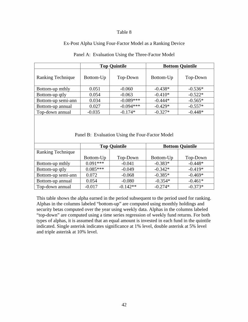
Table 8
Ex-Post Alpha Using Four-Factor Model as a Ranking Device
Panel A: Evaluation Using the Three-Factor Model
Top Quintile Bottom Quintile Ranking Technique
Bottom-Up
Top-Down
Bottom-Up
Top-Down
Bottom-up mthly 0.051 -0.060 -0.438* -0.536* Bottom-up qtly 0.054 -0.063 -0.410* -0.522* Bottom-up semi-ann 0.034 -0.089*** -0.444* -0.565* Bottom-up annual 0.027 -0.094*** -0.429* -0.557* Top-down annual -0.035 -0.174* -0.327* -0.448*
Panel B: Evaluation Using the Four-Factor Model
Top Quintile Bottom Quintile Ranking Technique
Bottom-Up
Top-Down
Bottom-Up
Top-Down
Bottom-up mthly 0.091*** -0.041 -0.383* -0.448* Bottom-up qtly 0.085*** -0.049 -0.342* -0.419* Bottom-up semi-ann 0.072 -0.068 -0.385* -0.469* Bottom-up annual 0.054 -0.080 -0.354* -0.461* Top-down annual -0.017 -0.142** -0.274* -0.373* This table shows the alpha earned in the period subsequent to the period used for ranking. Alphas in the columns labeled “bottom-up” are computed using monthly holdings and security betas computed over the year using weekly data. Alphas in the columns labeled “top-down” are computed using a time series regression of weekly fund returns. For both types of alphas, it is assumed that an equal amount is invested in each fund in the quintile indicated. Single asterisk indicates significance at 1% level, double asterisk at 5% level and triple asterisk at 10% level.
42

Table 9
Decile Alphas from Monthly Bottom-Up alphas
Decile Evaluated by Three-Index
Monthly Estimate
Evaluated by Four-Index
Monthly Estimate Top-Down Bottom-Up Bottom-Up 1 0.100 0.151 0.138 2 0.076 0.164 0.126 3 -0.083 0.010 0.045 4 -0.170 -0.020 -0.034 5 -0.071 0.072 0.033 6 -0.373 -0.216 -0.260 7 -0.301 -0.120 -0.082 8 -0.470 -0.214 -0.103 9 -0.551 -0.355 -0.334 10 -0.523 -0.472 -0.332
Spearman Rank Correlation
0.952*
0.915*
0.952*
* Significant at the 1% level. This table shows the average ex-post alpha in each decile where the ex-ante ranking is done on the basis of the monthly bottom-up alphas and evaluation is bottom-up monthly and top-down using the three-index model and bottom-up using the four-index model. This table presents realized alpha for the years 2002, 2003 and 2004.
43

Table 10
Ranking using Quarterly and Monthly G&T Measures; Evaluation Using G&T Measure and Three-Factor Alphas
G&T Rankings Quarterly Ranking Evaluated By: Monthly Ranking Evaluated By: G&T Bottom-up Top-down G&T Bottom-up Top-
down Top Quintile 0.027 -0.054 -0.236* 0.072** -0.201* -0.332* Bottom Quintile -0.007 -0.226* -0.315* -0.086* -0.182* * -0.284* Rank Correlation 0.430 0.261 0.200 0.891* 0.055 0.152
This table shows the performance in the next year when funds are ranked by the Grinblatt and Titman (G&T) measure. Performance is measured by the G&T measure and alpha computed using monthly holdings and betas computed using weekly data or alpha computed using weekly returns. An equal amount is assumed invested in each fund in the quintile. Single asterisk indicates significance at 1% level, double asterisk at 5% level and triple asterisk at 10% level.
44