moran, m.j. engineering thermodynamics mechanical … engineering... · moran, m.j. “engineering...
TRANSCRIPT

Moran, M.J. “Engineering Thermodynamics”Mechanical Engineering HandbookEd. Frank KreithBoca Raton: CRC Press LLC, 1999
c©1999 by CRC Press LLC
i
EngineeringThermodynamics
2.1 Fundamentals....................................................................2-2Basic Concepts and Definitions • The First Law of Thermodynamics, Energy • The Second Law of Thermodynamics, Entropy • Entropy and Entropy Generation
2.2 Control Volume Applications.........................................2-14Conservation of Mass • Control Volume Energy Balance • Control Volume Entropy Balance • Control Volumes at Steady State
2.3 Property Relations and Data..........................................2-22Basic Relations for Pure Substances • P-v-T Relations • Evaluating ∆h, ∆u, and ∆s • Fundamental Thermodynamic Functions • Thermodynamic Data Retrieval • Ideal Gas Model • Generalized Charts for Enthalpy, Entropy, and Fugacity • Multicomponent Systems
2.4 Combustion ....................................................................2-58Reaction Equations • Property Data for Reactive Systems • Reaction Equilibrium
2.5 Exergy Analysis..............................................................2-69Defining Exergy • Control Volume Exergy Rate Balance • Exergetic Efficiency • Exergy Costing
2.6 Vapor and Gas Power Cycles........................................2-78Rankine and Brayton Cycles • Otto, Diesel, and Dual Cycles • Carnot, Ericsson, and Stirling Cycles
2.7 Guidelines for Improving Thermodynamic Effectiveness...................................................................2-87
Although various aspects of what is now known as thermodynamics have been of interest since antiquity,formal study began only in the early 19th century through consideration of the motive power of heat:the capacity of hot bodies to produce work. Today the scope is larger, dealing generally with energy andentropy, and with relationships among the properties of matter. Moreover, in the past 25 years engineeringthermodynamics has undergone a revolution, both in terms of the presentation of fundamentals andnthe manner that it is applied. In particular, the second law of thermodynamics has emerged as an effectivetool for engineering analysis and design.
Michael J. MoranDepartment of Mechanical Engineering The Ohio State University
2-1© 1999 by CRC Press LLC
2
-2
Section 2
es theecules.antum
ormally fixed,
through
adefined
ol
sy some
ntropy for the
e
nating
When
ressed
operty
s to its
mpo-
e, a
2.1 Fundamentals
Classical thermodynamics is concerned primarily with the macrostructure of matter. It addressgross characteristics of large aggregations of molecules and not the behavior of individual molThe microstructure of matter is studied in kinetic theory and statistical mechanics (including quthermodynamics). In this chapter, the classical approach to thermodynamics is featured.
Basic Concepts and Definitions
Thermodynamics is both a branch of physics and an engineering science. The scientist is ninterested in gaining a fundamental understanding of the physical and chemical behavior ofquiescent quantities of matter and uses the principles of thermodynamics to relate the properties of matter.Engineers are generally interested in studying systems and how they interact with their surroundings. Tofacilitate this, engineers have extended the subject of thermodynamics to the study of systems which matter flows.
System
In a thermodynamic analysis, the system is the subject of the investigation. Normally the system isspecified quantity of matter and/or a region that can be separated from everything else by a well-surface. The defining surface is known as the control surface or system boundary. The control surfacemay be movable or fixed. Everything external to the system is the surroundings. A system of fixed massis referred to as a control mass or as a closed system. When there is flow of mass through the contrsurface, the system is called a control volume, or open, system. An isolated system is a closed systemthat does not interact in any way with its surroundings.
State, Property
The condition of a system at any instant of time is called its state. The state at a given instant of timeis described by the properties of the system. A property is any quantity whose numerical value dependon the state but not the history of the system. The value of a property is determined in principle btype of physical operation or test.
Extensive properties depend on the size or extent of the system. Volume, mass, energy, and eare examples of extensive properties. An extensive property is additive in the sense that its valuewhole system equals the sum of the values for its parts. Intensive properties are independent of the sizor extent of the system. Pressure and temperature are examples of intensive properties.
A mole is a quantity of substance having a mass numerically equal to its molecular weight. Desigthe molecular weight by M and the number of moles by n, the mass m of the substance is m = nM. Onekilogram mole, designated kmol, of oxygen is 32.0 kg and one pound mole (lbmol) is 32.0 lb. an extensive property is reported on a unit mass or a unit mole basis, it is called a specific property. Anoverbar is used to distinguish an extensive property written on a per-mole basis from its value expper unit mass. For example, the volume per mole is , whereas the volume per unit mass is v, and thetwo specific volumes are related by = Mv.
Process, Cycle
Two states are identical if, and only if, the properties of the two states are identical. When any prof a system changes in value there is a change in state, and the system is said to undergo aprocess.When a system in a given initial state goes through a sequence of processes and finally returninitial state, it is said to have undergone a cycle.
Phase and Pure Substance
The term phase refers to a quantity of matter that is homogeneous throughout in both chemical cosition and physical structure. Homogeneity in physical structure means that the matter is all solid, or allliquid, or all vapor (or equivalently all gas). A system can contain one or more phases. For exampl
vv
© 1999 by CRC Press LLC
Engineering Thermodynamics
2
-3
butr vapor phase has
alancepect of
,
fes of
ows:ere ared. The
internally all suchniformlumn
namicswingetween
here
ature
nith the
r,tween
system of liquid water and water vapor (steam) contains two phases. A pure substance is one that isuniform and invariable in chemical composition. A pure substance can exist in more than one phase,its chemical composition must be the same in each phase. For example, if liquid water and wateform a system with two phases, the system can be regarded as a pure substance because eachthe same composition. The nature of phases that coexist in equilibrium is addressed by the phase rule(Section 2.3, Multicomponent Systems).
Equilibrium
Equilibrium means a condition of balance. In thermodynamics the concept includes not only a bof forces, but also a balance of other influences. Each kind of influence refers to a particular asthermodynamic (complete) equilibrium. Thermal equilibrium refers to an equality of temperaturemechanical equilibrium to an equality of pressure, and phase equilibrium to an equality of chemicalpotentials (Section 2.3, Multicomponent Systems). Chemical equilibrium is also established in terms ochemical potentials (Section 2.4, Reaction Equilibrium). For complete equilibrium the several typequilibrium must exist individually.
To determine if a system is in thermodynamic equilibrium, one may think of testing it as follisolate the system from its surroundings and watch for changes in its observable properties. If thno changes, it may be concluded that the system was in equilibrium at the moment it was isolatesystem can be said to be at an equilibrium state. When a system is isolated, it cannot interact with itssurroundings; however, its state can change as a consequence of spontaneous events occurring as its intensive properties, such as temperature and pressure, tend toward uniform values. Whenchanges cease, the system is in equilibrium. At equilibrium. temperature and pressure are uthroughout. If gravity is significant, a pressure variation with height can exist, as in a vertical coof liquid.
Temperature
A scale of temperature independent of the thermometric substance is called a thermodynamic temperaturescale. The Kelvin scale, a thermodynamic scale, can be elicited from the second law of thermody(Section 2.1, The Second Law of Thermodynamics, Entropy). The definition of temperature follofrom the second law is valid over all temperature ranges and provides an essential connection bthe several empirical measures of temperature. In particular, temperatures evaluated using a constant-volume gas thermometer are identical to those of the Kelvin scale over the range of temperatures wgas thermometry can be used.
The empirical gas scale is based on the experimental observations that (1) at a given temperlevel all gases exhibit the same value of the product (p is pressure and the specific volume oa molar basis) if the pressure is low enough, and (2) the value of the product increases wtemperature level. On this basis the gas temperature scale is defined by
where T is temperature and is the universal gas constant. The absolute temperature at the triple pointof water (Section 2.3, P-v-T Relations) is fixed by international agreement to be 273.16 K on the Kelvintemperature scale. is then evaluated experimentally as= 8.314 kJ/kmol · K (1545 ft · lbf/lbmol · °R).
The Celsius termperature scale (also called the centigrade scale) uses the degree Celsius (°C), whichhas the same magnitude as the kelvin. Thus, temperature differences are identical on both scales. Howevethe zero point on the Celsius scale is shifted to 273.15 K, as shown by the following relationship bethe Celsius temperature and the Kelvin temperature:
(2.1)
On the Celsius scale, the triple point of water is 0.01°C and 0 K corresponds to –273.15°C.
pv vpv
TR
pvp
= ( )→
10
lim
R
R R
T T°( ) = ( ) −C K 273 15.
© 1999 by CRC Press LLC
2
-4
Section 2
to
es with terms
point
racticalhat the is thef ITS-
f engi-y,
oneundingstanged,
ld haveoncept shafts,
:gn
dings
Two other temperature scales are commonly used in engineering in the U.S. By definition, the Rankinescale, the unit of which is the degree rankine (°R), is proportional to the Kelvin temperature according
(2.2)
The Rankine scale is also an absolute thermodynamic scale with an absolute zero that coincidthe absolute zero of the Kelvin scale. In thermodynamic relationships, temperature is always inof the Kelvin or Rankine scale unless specifically stated otherwise.
A degree of the same size as that on the Rankine scale is used in the Fahrenheit scale, but the zeropoint is shifted according to the relation
(2.3)
Substituting Equations 2.1 and 2.2 into Equation 2.3 gives
(2.4)
This equation shows that the Fahrenheit temperature of the ice point (0°C) is 32°F and of the steampoint (100°C) is 212°F. The 100 Celsius or Kelvin degrees between the ice point and steam corresponds to 180 Fahrenheit or Rankine degrees.
To provide a standard for temperature measurement taking into account both theoretical and pconsiderations, the International Temperature Scale of 1990 (ITS-90) is defined in such a way ttemperature measured on it conforms with the thermodynamic temperature, the unit of whichkelvin, to within the limits of accuracy of measurement obtainable in 1990. Further discussion o90 is provided by Preston-Thomas (1990).
The First Law of Thermodynamics, Energy
Energy is a fundamental concept of thermodynamics and one of the most significant aspects oneering analysis. Energy can be stored within systems in various macroscopic forms: kinetic energgravitational potential energy, and internal energy. Energy can also be transformed from one form toanother and transferred between systems. For closed systems, energy can be transferred by work andheat transfer. The total amount of energy is conserved in all transformations and transfers.
Work
In thermodynamics, the term work denotes a means for transferring energy. Work is an effect of system on another that is identified and measured as follows: work is done by a system on its surroif the sole effect on everything external to the system could have been the raising of a weight. The tesof whether a work interaction has taken place is not that the elevation of a weight is actually chnor that a force actually acted through a distance, but that the sole effect could be the change in elevationof a mass. The magnitude of the work is measured by the number of standard weights that coubeen raised. Since the raising of a weight is in effect a force acting through a distance, the work cof mechanics is preserved. This definition includes work effects such as is associated with rotatingdisplacement of the boundary, and the flow of electricity.
Work done by a system is considered positive: W > 0. Work done on a system is considered negativeW < 0. The time rate of doing work, or power, is symbolized by and adheres to the same siconvention.
Energy
A closed system undergoing a process that involves only work interactions with its surrounexperiences an adiabatic process. On the basis of experimental evidence, it can be postulated thatwhen
T T°( ) = ( )R K1 8.
T T°( ) = °( ) −F R 459 67.
T T°( ) = °( ) +F C1 8 32.
W
© 1999 by CRC Press LLC
Engineering Thermodynamics 2-5
tem and
pe of
propertyk in ange in then ,
energy
rk terman bed to the
urface)
s work,contacts
systemadiabatic
transfer.
a closed system is altered adiabatically, the amount of work is fixed by the end states of the sysis independent of the details of the process. This postulate, which is one way the first law of thermody-namics can be stated, can be made regardless of the type of work interaction involved, the typrocess, or the nature of the system.
As the work in an adiabatic process of a closed system is fixed by the end states, an extensive called energy can be defined for the system such that its change between two states is the woradiabatic process that has these as the end states. In engineering thermodynamics the chanenergy of a system is considered to be made up of three macroscopic contributions: the change ikineticenergy, KE, associated with the motion of the system as a whole relative to an external coordinate framethe change in gravitational potential energy, PE, associated with the position of the system as a wholein the Earth’s gravitational field, and the change in internal energy, U, which accounts for all otherenergy associated with the system. Like kinetic energy and gravitational potential energy, internal is an extensive property.
In summary, the change in energy between two states of a closed system in terms of the workWad ofan adiabatic process between these states is
(2.5)
where 1 and 2 denote the initial and final states, respectively, and the minus sign before the wois in accordance with the previously stated sign convention for work. Since any arbitrary value cassigned to the energy of a system at a given state 1, no particular significance can be attachevalue of the energy at state 1 or at any other state. Only changes in the energy of a system havesignificance.
The specific energy (energy per unit mass) is the sum of the specific internal energy, u, the specifickinetic energy, v2/2, and the specific gravitational potential energy, gz, such that
(2.6)
where the velocity v and the elevation z are each relative to specified datums (often the Earth’s sand g is the acceleration of gravity.
A property related to internal energy u, pressure p, and specific volume v is enthalpy, defined by
(2.7a)
or on an extensive basis
(2.7b)
Heat
Closed systems can also interact with their surroundings in a way that cannot be categorized aas, for example, a gas (or liquid) contained in a closed vessel undergoing a process while in with a flame. This type of interaction is called a heat interaction, and the process is referred to anonadiabatic.
A fundamental aspect of the energy concept is that energy is conserved. Thus, since a closedexperiences precisely the same energy change during a nonadiabatic process as during an process between the same end states, it can be concluded that the net energy transfer to the system ineach of these processes must be the same. It follows that heat interactions also involve energy
KE KE PE PE U U Wad2 1 2 1 2 1−( ) + −( ) + −( ) = −
specific energyv
gz= + +u2
2
h u pv= +
H U pV= +
© 1999 by CRC Press LLC
2-6 Section 2
stems of
osedat such and itstransfer
ethods
tchieved.
.8 reads
e netteat.
total
Denoting the amount of energy transferred to a closed system in heat interactions by Q, these consid-erations can be summarized by the closed system energy balance:
(2.8)
The closed system energy balance expresses the conservation of energy principle for closed syall kinds.
The quantity denoted by Q in Equation 2.8 accounts for the amount of energy transferred to a clsystem during a process by means other than work. On the basis of experiments it is known than energy transfer is induced only as a result of a temperature difference between the systemsurroundings and occurs only in the direction of decreasing temperature. This means of energy is called an energy transfer by heat. The following sign convention applies:
The time rate of heat transfer, denoted by , adheres to the same sign convention.Methods based on experiment are available for evaluating energy transfer by heat. These m
recognize two basic transfer mechanisms: conduction and thermal radiation. In addition, theoretical andempirical relationships are available for evaluating energy transfer involving combined modes such asconvection. Further discussion of heat transfer fundamentals is provided in Chapter 4.
The quantities symbolized by W and Q account for transfers of energy. The terms work and heatdenote different means whereby energy is transferred and not what is transferred. Work and heat are noproperties, and it is improper to speak of work or heat “contained” in a system. However, to aeconomy of expression in subsequent discussions, W and Q are often referred to simply as work anheat transfer, respectively. This less formal approach is commonly used in engineering practice
Power Cycles
Since energy is a property, over each cycle there is no net change in energy. Thus, Equation 2for any cycle
That is, for any cycle the net amount of energy received through heat interactions is equal to thenergy transferred out in work interactions. A power cycle, or heat engine, is one for which a net amounof energy is transferred out by work: Wcycle > 0. This equals the net amount of energy transferred in by h
Power cycles are characterized both by addition of energy by heat transfer, QA, and inevitable rejectionsof energy by heat transfer, QR:
Combining the last two equations,
The thermal efficiency of a heat engine is defined as the ratio of the net work developed to theenergy added by heat transfer:
U U KE KE PE PE Q W2 1 2 1 2 1−( ) + −( ) + −( ) = −
Q to
Q from
>
<
0
0
:
:
heat transfer the system
heat transfer the system
Q
Q Wcycle cycle=
Q Q Qcycle A R= −
W Q Qcycle A R= −
© 1999 by CRC Press LLC
Engineering Thermodynamics 2-7
be calledid.ctly by
al law,
oved by numbertensiveystems
dings
t is
ngle
ibilities
ere
ichem thatal state.rn the
de, butainedatter attricforma-
n theof thein the
(2.9)
The thermal efficiency is strictly less than 100%. That is, some portion of the energy QA supplied isinvariably rejected QR ≠ 0.
The Second Law of Thermodynamics, Entropy
Many statements of the second law of thermodynamics have been proposed. Each of these can a statement of the second law or a corollary of the second law since, if one is invalid, all are invalIn every instance where a consequence of the second law has been tested directly or indireexperiment it has been verified. Accordingly, the basis of the second law, like every other physicis experimental evidence.
Kelvin-Planck Statement
The Kelvin-Plank statement of the second law of thermodynamics refers to a thermal reservoir. A thermalreservoir is a system that remains at a constant temperature even though energy is added or remheat transfer. A reservoir is an idealization, of course, but such a system can be approximated in aof ways — by the Earth’s atmosphere, large bodies of water (lakes, oceans), and so on. Exproperties of thermal reservoirs, such as internal energy, can change in interactions with other seven though the reservoir temperature remains constant, however.
The Kelvin-Planck statement of the second law can be given as follows: It is impossible for any systemto operate in a thermodynamic cycle and deliver a net amount of energy by work to its surrounwhile receiving energy by heat transfer from a single thermal reservoir. In other words, a perpetual-motion machine of the second kind is impossible. Expressed analytically, the Kelvin-Planck statemen
where the words single reservoir emphasize that the system communicates thermally only with a sireservoir as it executes the cycle. The “less than” sign applies when internal irreversibilities are presentas the system of interest undergoes a cycle and the “equal to” sign applies only when no irreversare present.
Irreversibilities
A process is said to be reversible if it is possible for its effects to be eradicated in the sense that this some way by which both the system and its surroundings can be exactly restored to their respectiveinitial states. A process is irreversible if there is no way to undo it. That is, there is no means by whthe system and its surroundings can be exactly restored to their respective initial states. A systhas undergone an irreversible process is not necessarily precluded from being restored to its initiHowever, were the system restored to its initial state, it would not also be possible to retusurroundings to their initial state.
There are many effects whose presence during a process renders it irreversible. These incluare not limited to, the following: heat transfer through a finite temperature difference; unrestrexpansion of a gas or liquid to a lower pressure; spontaneous chemical reaction; mixing of mdifferent compositions or states; friction (sliding friction as well as friction in the flow of fluids); eleccurrent flow through a resistance; magnetization or polarization with hysteresis; and inelastic detion. The term irreversibility is used to identify effects such as these.
Irreversibilities can be divided into two classes, internal and external. Internal irreversibilities arethose that occur within the system, while external irreversibilities are those that occur withisurroundings, normally the immediate surroundings. As this division depends on the location boundary there is some arbitrariness in the classification (by locating the boundary to take
η = = −W
Q
Q
Qcycle
A
R
A
1
Wcycle ≤ ( )0 single reservoir
© 1999 by CRC Press LLC
2-8 Section 2
ent:
.a
.
er
t
e
immediate surroundings, all irreversibilities are internal). Nonetheless, valuable insights can result whenthis distinction between irreversibilities is made. When internal irreversibilities are absent during aprocess, the process is said to be internally reversible. At every intermediate state of an internallyreversible process of a closed system, all intensive properties are uniform throughout each phase presthe temperature, pressure, specific volume, and other intensive properties do not vary with position. Thediscussions to follow compare the actual and internally reversible process concepts for two cases ofspecial interest.
For a gas as the system, the work of expansion arises from the force exerted by the system to movethe boundary against the resistance offered by the surroundings:
where the force is the product of the moving area and the pressure exerted by the system there. Notingthat Adx is the change in total volume of the system,
This expression for work applies to both actual and internally reversible expansion processes. However,for an internally reversible process p is not only the pressure at the moving boundary but also the pressureof the entire system. Furthermore, for an internally reversible process the volume equals mv, where thespecific volume v has a single value throughout the system at a given instant. Accordingly, the work ofan internally reversible expansion (or compression) process is
(2.10)
When such a process of a closed system is represented by a continuous curve on a plot of pressure vsspecific volume, the area under the curve is the magnitude of the work per unit of system mass (area-b-c′-d′ of Figure 2.3, for example).
Although improved thermodynamic performance can accompany the reduction of irreversibilities,steps in this direction are normally constrained by a number of practical factors often related to costsFor example, consider two bodies able to communicate thermally. With a finite temperature differencebetween them, a spontaneous heat transfer would take place and, as noted previously, this would be asource of irreversibility. The importance of the heat transfer irreversibility diminishes as the temperaturdifference narrows; and as the temperature difference between the bodies vanishes, the heat transfeapproaches ideality. From the study of heat transfer it is known, however, that the transfer of a finiteamount of energy by heat between bodies whose temperatures differ only slightly requires a considerableamount of time, a large heat transfer surface area, or both. To approach ideality, therefore, a heat transferwould require an exceptionally long time and/or an exceptionally large area, each of which has cosimplications constraining what can be achieved practically.
Carnot Corollaries
The two corollaries of the second law known as Carnot corollaries state: (1) the thermal efficiency ofan irreversible power cycle is always less than the thermal efficiency of a reversible power cycle wheneach operates between the same two thermal reservoirs; (2) all reversible power cycles operating betweenthe same two thermal reservoirs have the same thermal efficiency. A cycle is considered reversible whenthere are no irreversibilities within the system as it undergoes the cycle, and heat transfers between thsystem and reservoirs occur ideally (that is, with a vanishingly small temperature difference).
W Fdx pAdx= =∫ ∫1
2
1
2
W pdV= ∫1
2
W m pdv= ∫1
2
© 1999 by CRC Press LLC
Engineering Thermodynamics 2-9
tweene of the.9 it canpendent
eratingons for
pletede used tosibleoir at any
d that is
eratures
n
on thepplied
Kelvin Temperature Scale
Carnot corollary 2 suggests that the thermal efficiency of a reversible power cycle operating betwo thermal reservoirs depends only on the temperatures of the reservoirs and not on the natursubstance making up the system executing the cycle or the series of processes. With Equation 2be concluded that the ratio of the heat transfers is also related only to the temperatures, and is indeof the substance and processes:
where QH is the energy transferred to the system by heat transfer from a hot reservoir at temperatureTH, and QC is the energy rejected from the system to a cold reservoir at temperature TC. The words revcycle emphasize that this expression applies only to systems undergoing reversible cycles while opbetween the two reservoirs. Alternative temperature scales correspond to alternative specificatithe function ψ in this relation.
The Kelvin temperature scale is based on ψ(TC, TH) = TC/TH. Then
(2.11)
This equation defines only a ratio of temperatures. The specification of the Kelvin scale is comby assigning a numerical value to one standard reference state. The state selected is the samdefine the gas scale: at the triple point of water the temperature is specified to be 273.16 K. If a revercycle is operated between a reservoir at the reference-state temperature and another reservunknown temperature T, then the latter temperature is related to the value at the reference state b
where Q is the energy received by heat transfer from the reservoir at temperature T, and Q′ is the energyrejected to the reservoir at the reference temperature. Accordingly, a temperature scale is definevalid over all ranges of temperature and that is independent of the thermometric substance.
Carnot Efficiency
For the special case of a reversible power cycle operating between thermal reservoirs at tempTH and TC on the Kelvin scale, combination of Equations 2.9 and 2.11 results in
(2.12)
called the Carnot efficiency. This is the efficiency of all reversible power cycles operating betweethermal reservoirs at TH and TC. Moreover, it is the maximum theoretical efficiency that any power cycle,real or ideal, could have while operating between the same two reservoirs. As temperatures Rankine scale differ from Kelvin temperatures only by the factor 1.8, the above equation may be awith either scale of temperature.
Q
QT TC
H revcycle
C H
= ( )ψ ,
Q
Q
T
TC
H revcycle
C
H
=
TQ
Q revcycle
=′
273 16.
ηmax = −1T
TC
H
© 1999 by CRC Press LLC
2-10 Section 2
tive
cycle,
ithstemof the-Plancks whens when
d canem
process1. The samee form
esses.
The Clausius Inequality
The Clausius inequality provides the basis for introducing two ideas instrumental for quantitaevaluations of processes of systems from a second law perspective: entropy and entropy generation. TheClausius inequality states that
(2.13a)
where δQ represents the heat transfer at a part of the system boundary during a portion of theand T is the absolute temperature at that part of the boundary. The symbol δ is used to distinguish thedifferentials of nonproperties, such as heat and work, from the differentials of properties, written wthe symbol d. The subscript b indicates that the integrand is evaluated at the boundary of the syexecuting the cycle. The symbol indicates that the integral is to be performed over all parts boundary and over the entire cycle. The Clausius inequality can be demonstrated using the Kelvinstatement of the second law, and the significance of the inequality is the same: the equality appliethere are no internal irreversibilities as the system executes the cycle, and the inequality applieinternal irreversibilities are present.
The Clausius inequality can be expressed alternatively as
(2.13b)
where Sgen can be viewed as representing the strength of the inequality. The value of Sgen is positivewhen internal irreversibilities are present, zero when no internal irreversibilities are present, annever be negative. Accordingly, Sgen is a measure of the irreversibilities present within the systexecuting the cycle. In the next section, Sgen is identified as the entropy generated (or produced) byinternal irreversibilities during the cycle.
Entropy and Entropy Generation
Entropy
Consider two cycles executed by a closed system. One cycle consists of an internally reversible A from state 1 to state 2, followed by an internally reversible process C from state 2 to state other cycle consists of an internally reversible process B from state 1 to state 2, followed by theprocess C from state 2 to state 1 as in the first cycle. For these cycles, Equation 2.13b takes th
where Sgen has been set to zero since the cycles are composed of internally reversible procSubtracting these equations leaves
δQ
T b
≤∫ 0
∫
δQ
TS
bgen
= −∫
δ δ
δ δ
Q
T
Q
TS
Q
T
Q
TS
A Cgen
B Cgen
1
2
2
1
1
2
2
1
0
0
∫ ∫
∫ ∫
+
= − =
+
= − =
δ δQ
T
Q
TA B1
2
1
2
∫ ∫
=
© 1999 by CRC Press LLC
Engineering Thermodynamics 2-11
s only. Itelecting
cess
ther is other
de of the
s
he
entropy,
bilitiesb takes
ersiblerm only.
Since A and B are arbitrary, it follows that the integral of δQ/T has the same value for any internallyreversible process between the two states: the value of the integral depends on the end statecan be concluded, therefore, that the integral defines the change in some property of the system. Sthe symbol S to denote this property, its change is given by
(2.14a)
where the subscript int rev indicates that the integration is carried out for any internally reversible prolinking the two states. This extensive property is called entropy.
Since entropy is a property, the change in entropy of a system in going from one state to anothe same for all processes, both internally reversible and irreversible, between these two states. Inwords, once the change in entropy between two states has been evaluated, this is the magnituentropy change for any process of the system between these end states.
The definition of entropy change expressed on a differential basis is
(2.14b)
Equation 2.14b indicates that when a closed system undergoing an internally reversible process receivesenergy by heat transfer, the system experiences an increase in entropy. Conversely, when energy iremoved from the system by heat transfer, the entropy of the system decreases. This can be interpretedto mean that an entropy transfer is associated with (or accompanies) heat transfer. The direction of tentropy transfer is the same as that of the heat transfer. In an adiabatic internally reversible process ofa closed system the entropy would remain constant. A constant entropy process is called an isentropicprocess.
On rearrangement, Equation 2.14b becomes
Then, for an internally reversible process of a closed system between state 1 and state 2,
(2.15)
When such a process is represented by a continuous curve on a plot of temperature vs. specificthe area under the curve is the magnitude of the heat transfer per unit of system mass.
Entropy Balance
For a cycle consisting of an actual process from state 1 to state 2, during which internal irreversiare present, followed by an internally reversible process from state 2 to state 1, Equation 2.13the form
where the first integral is for the actual process and the second integral is for the internally revprocess. Since no irreversibilities are associated with the internally reversible process, the teSgen
accounting for the effect of irreversibilities during the cycle can be identified with the actual process
S SQ
Trev
2 11
2
− =
∫ δ
int
dSQ
Trev
=
δint
δQ TdSrev
( ) =int
Q m Tdsrevint = ∫1
2
δ δQ
T
Q
TS
b rev
gen
+
= −∫ ∫1
2
2
1
int
© 1999 by CRC Press LLC
2-12 Section 2
n be
valuatede rightdge ofsystemg)nd therred into
e to the
absent.nopy is. Sinceepends
term.ot havemple,
valuesparing
entifiedheavily
oth the transfer eitherlibrium.ugh of
largedin the
Applying the definition of entropy change, the second integral of the foregoing equation caexpressed as
Introducing this and rearranging the equation, the closed system entropy balance results:
(2.16)
When the end states are fixed, the entropy change on the left side of Equation 2.16 can be eindependently of the details of the process from state 1 to state 2. However, the two terms on thside depend explicitly on the nature of the process and cannot be determined solely from knowlethe end states. The first term on the right side is associated with heat transfer to or from the during the process. This term can be interpreted as the entropy transfer associated with (or accompanyinheat transfer. The direction of entropy transfer is the same as the direction of the heat transfer, asame sign convention applies as for heat transfer: a positive value means that entropy is transfethe system, and a negative value means that entropy is transferred out.
The entropy change of a system is not accounted for solely by entropy transfer, but is also dusecond term on the right side of Equation 2.16 denoted by Sgen. The term Sgen is positive when internalirreversibilities are present during the process and vanishes when internal irreversibilities are This can be described by saying that entropy is generated (or produced) within the system by the actioof irreversibilities. The second law of thermodynamics can be interpreted as specifying that entrgenerated by irreversibilities and conserved only in the limit as irreversibilities are reduced to zeroSgen measures the effect of irreversibilities present within a system during a process, its value don the nature of the process and not solely on the end states. Entropy generation is not a property.
When applying the entropy balance, the objective is often to evaluate the entropy generationHowever, the value of the entropy generation for a given process of a system usually does nmuch significance by itself. The significance is normally determined through comparison. For exathe entropy generation within a given component might be compared to the entropy generationof the other components included in an overall system formed by these components. By comentropy generation values, the components where appreciable irreversibilities occur can be idand rank ordered. This allows attention to be focused on the components that contribute most to inefficient operation of the overall system.
To evaluate the entropy transfer term of the entropy balance requires information regarding bheat transfer and the temperature on the boundary where the heat transfer occurs. The entropyterm is not always subject to direct evaluation, however, because the required information isunknown or undefined, such as when the system passes through states sufficiently far from equiIn practical applications, it is often convenient, therefore, to enlarge the system to include enothe immediate surroundings that the temperature on the boundary of the enlarged system correspondsto the ambient temperature, Tamb. The entropy transfer term is then simply Q/Tamb. However, as theirreversibilities present would not be just those for the system of interest but those for the ensystem, the entropy generation term would account for the effects of internal irreversibilities with
S SQ
Trev
1 22
1
− =
∫ δ
int
S SQ
TS
bgen2 1
1
2
− =
+∫ δ
______ ______ ______
entropy
change
entropy
transfer
entropy
generation
© 1999 by CRC Press LLC
Engineering Thermodynamics 2-13
the
time m.
eratedhose for
system and external irreversibilities present within that portion of the surroundings included withinenlarged system.
A form of the entropy balance convenient for particular analyses is the rate form:
(2.17)
where dS/dt is the time rate of change of entropy of the system. The term represents therate of entropy transfer through the portion of the boundary whose instantaneous temperature isTj. Theterm accounts for the time rate of entropy generation due to irreversibilities within the syste
For a system isolated from its surroundings, the entropy balance is
(2.18)
where Sgen is the total amount of entropy generated within the isolated system. Since entropy is genin all actual processes, the only processes of an isolated system that actually can occur are twhich the entropy of the isolated system increases. This is known as the increase of entropy principle.
dS
dt
Q
TSj
jgen
j
= +∑˙
˙
˙ /Q Tj j
Sgen
S S Sisol gen2 1−( ) =
© 1999 by CRC Press LLC
2-14 Section 2
sis, thetion arere (see,
flow innd
rinciple
control
plicity.
ate ofely, for
2.2 Control Volume Applications
Since most applications of engineering thermodynamics are conducted on a control volume bacontrol volume formulations of the mass, energy, and entropy balances presented in this secespecially important. These are given here in the form of overall balances. Equations of change fomass, energy, and entropy in the form of differential equations are also available in the literature.g., Bird et al., 1960).
Conservation of Mass
When applied to a control volume, the principle of mass conservation states: The time rate of accumu-lation of mass within the control volume equals the difference between the total rates of mass and out across the boundary. An important case for engineering practice is one for which inward aoutward flows occur, each through one or more ports. For this case the conservation of mass ptakes the form
(2.19)
The left side of this equation represents the time rate of change of mass contained within the volume, denotes the mass flow rate at an inlet, and is the mass flow rate at an outlet.
The volumetric flow rate through a portion of the control surface with area dA is the product of thevelocity component normal to the area, vn, times the area: vn dA. The mass flow rate through dA is ρ(vn
dA). The mass rate of flow through a port of area A is then found by integration over the area
For one-dimensional flow the intensive properties are uniform with position over area A, and the lastequation becomes
(2.20)
where v denotes the specific volume and the subscript n has been dropped from velocity for sim
Control Volume Energy Balance
When applied to a control volume, the principle of energy conservation states: The time rate of accu-mulation of energy within the control volume equals the difference between the total incoming renergy transfer and the total outgoing rate of energy transfer. Energy can enter and exit a control volumby work and heat transfer. Energy also enters and exits with flowing streams of matter. Accordinga control volume with one-dimensional flow at a single inlet and a single outlet,
(2.21)
dm
dtm mcv
i
i
e
e
= −∑ ∑˙ ˙
mi me
m dAA
= ∫ ρvn
m AA
v= =ρv
v
d U KE PE
dtQ W m u m ucv
cv ii
i ee
e
+ +( )= − + + +
− + +
˙ ˙ ˙ ˙
___________ ___________
vgz
vgz
2 2
2 2
© 1999 by CRC Press LLC
Engineering Thermodynamics 2-15
s. Thever the
ary, theiatede other,lace-f these
(with
and
mass
timel ratesnd work,
can berencebtained
where the underlined terms account for the specific energy of the incoming and outgoing streamterms and account, respectively, for the net rates of energy transfer by heat and work oboundary (control surface) of the control volume.
Because work is always done on or by a control volume where matter flows across the boundquantity of Equation 2.21 can be expressed in terms of two contributions: one is the work assocwith the force of the fluid pressure as mass is introduced at the inlet and removed at the exit. Thdenoted as , includes all other work effects, such as those associated with rotating shafts, dispment of the boundary, and electrical effects. The work rate concept of mechanics allows the first ocontributions to be evaluated in terms of the product of the pressure force, pA, and velocity at the pointof application of the force. To summarize, the work term of Equation 2.21 can be expressedEquation 2.20) as
(2.22)
The terms (pvi) and (peve) account for the work associated with the pressure at the inlet outlet, respectively, and are commonly referred to as flow work.
Substituting Equation 2.22 into Equation 2.21, and introducing the specific enthalpy h, the followingform of the control volume energy rate balance results:
(2.23)
To allow for applications where there may be several locations on the boundary through whichenters or exits, the following expression is appropriate:
(2.24)
Equation 2.24 is an accounting rate balance for the energy of the control volume. It states that the rate of accumulation of energy within the control volume equals the difference between the totaof energy transfer in and out across the boundary. The mechanisms of energy transfer are heat aas for closed systems, and the energy accompanying the entering and exiting mass.
Control Volume Entropy Balance
Like mass and energy, entropy is an extensive property. And like mass and energy, entropy transferred into or out of a control volume by streams of matter. As this is the principal diffebetween the closed system and control volume forms, the control volume entropy rate balance is oby modifying Equation 2.17 to account for these entropy transfers. The result is
(2.25)
Qcv W
W
Wcv
W
˙ ˙
˙ ˙ ˙
W W p A p A
W m p v m p v
cv e e e i i i
cv e e e i i i
= + ( ) − ( )= + ( ) − ( )
v v
mi me
d U KE PE
dtQ W m h m hcv
cv cv i ii
i e ee
e
+ +( )= − + + +
− + +
˙ ˙ ˙ ˙v
gzv
gz2 2
2 2
d U KE PE
dtQ W m h m hcv
cv cv i
i
ii
i e
e
ee
e
+ +( )= − + + +
− + +
∑ ∑˙ ˙ ˙ ˙
vgz
vgz
2 2
2 2
dS
dt
Q
Tm s m s Scv j
jj
i
i
i e e
e
gen= + − +∑ ∑ ∑˙
˙ ˙ ˙
_____ ______________________ _________
rate of
entropy
change
rate of
entropy
transfer
rate of
entropy
generation
© 1999 by CRC Press LLC
2-16 Section 2
re i
g-
r
where dScv/dt represents the time rate of change of entropy within the control volume. The terms andaccount, respectively, for rates of entropy transfer into and out of the control volume associated
with mass flow. One-dimensional flow is assumed at locations where mass enters and exits. representsthe time rate of heat transfer at the location on the boundary where the instantaneous temperatus Tj;and accounts for the associated rate of entropy transfer. denotes the time rate of entropygeneration due to irreversibilities within the control volume. When a control volume comprises a numberof components, is the sum of the rates of entropy generation of the components.
Control Volumes at Steady State
Engineering systems are often idealized as being at steady state, meaning that all properties are unchaning in time. For a control volume at steady state, the identity of the matter within the control volumechange continuously, but the total amount of mass remains constant. At steady state, Equation 2.19reduces to
(2.26a)
The energy rate balance of Equation 2.24 becomes, at steady state,
(2.26b)
At steady state, the entropy rate balance of Equation 2.25 reads
(2.26c)
Mass and energy are conserved quantities, but entropy is not generally conserved. Equation 2.26aindicates that the total rate of mass flow into the control volume equals the total rate of mass flow outof the control volume. Similarly, Equation 2.26b states that the total rate of energy transfer into thecontrol volume equals the total rate of energy transfer out of the control volume. However, Equation2.26c shows that the rate at which entropy is transferred out exceeds the rate at which entropy enters,the difference being the rate of entropy generation within the control volume owing to irreversibilities.
Applications frequently involve control volumes having a single inlet and a single outlet, as, foexample, the control volume of Figure 2.1 where heat transfer (if any) occurs at Tb: the temperature, ora suitable average temperature, on the boundary where heat transfer occurs. For this case the mass ratebalance, Equation 2.26a, reduces to Denoting the common mass flow rate by Equations2.26b and 2.26c read, respectively,
(2.27a)
(2.28a)
When Equations 2.27a and 2.28a are applied to particular cases of interest, additional simplificationsare usually made. The heat transfer term is dropped when it is insignificant relative to other energy
m si i
m se e
Qj
˙ /Q Tj j Sgen
Sgen
˙ ˙m mi
i
e
e∑ ∑=
02 2
2 2
= − + + +
− + +
∑ ∑˙ ˙ ˙ ˙Q W m h m hcv cv i
i
ii
i e
e
ee
e
vgz
vgz
0 = + − +∑ ∑ ∑˙
˙ ˙ ˙Q
Tm s m s Sj
jj
i
i
i e e
e
gen
˙ ˙ .m mi e= ˙ ,m
02
2 2
= − + −( ) +−
+ −( )
˙ ˙ ˙Q W m h hcv cv i ei e
i e
v vg z z
0 = + −( ) +˙
˙ ˙Q
Tm s s Scv
bi e gen
Qcv
© 1999 by CRC Press LLC
Engineering Thermodynamics 2-17
ll
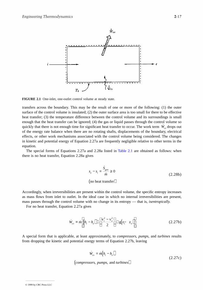
transfers across the boundary. This may be the result of one or more of the following: (1) the outersurface of the control volume is insulated; (2) the outer surface area is too small for there to be effectiveheat transfer; (3) the temperature difference between the control volume and its surroundings is smaenough that the heat transfer can be ignored; (4) the gas or liquid passes through the control volume soquickly that there is not enough time for significant heat transfer to occur. The work term drops outof the energy rate balance when there are no rotating shafts, displacements of the boundary, electricaleffects, or other work mechanisms associated with the control volume being considered. The changesin kinetic and potential energy of Equation 2.27a are frequently negligible relative to other terms in theequation.
The special forms of Equations 2.27a and 2.28a listed in Table 2.1 are obtained as follows: whenthere is no heat transfer, Equation 2.28a gives
(2.28b)
Accordingly, when irreversibilities are present within the control volume, the specific entropy increasesas mass flows from inlet to outlet. In the ideal case in which no internal irreversibilities are present,mass passes through the control volume with no change in its entropy — that is, isentropically.
For no heat transfer, Equation 2.27a gives
(2.27b)
A special form that is applicable, at least approximately, to compressors, pumps, and turbines resultsfrom dropping the kinetic and potential energy terms of Equation 2.27b, leaving
(2.27c)
FIGURE 2.1 One-inlet, one-outlet control volume at steady state.
Wcv
s sS
me igen− = ≥
( )
˙
˙0
no heat transfer
˙ ˙W m h hcv i ei e
i e= −( ) +−
+ −( )
v vg z z
2 2
2
˙ ˙W m h h
compressors pumps turbines
cv i e= −( )( ), , and
© 1999 by CRC Press LLC
2-18 Section 2
s
In throttling devices a significant reduction in pressure is achieved simply by introducing a restrictioninto a line through which a gas or liquid flows. For such devices = 0 and Equation 2.27c reducefurther to read(2.27d)
That is, upstream and downstream of the throttling device, the specific enthalpies are equal.A nozzle is a flow passage of varying cross-sectional area in which the velocity of a gas or liquid
increases in the direction of flow. In a diffuser, the gas or liquid decelerates in the direction of flow. Forsuch devices, = 0. The heat transfer and potential energy change are also generally negligible. ThenEquation 2.27b reduces to
(2.27e)
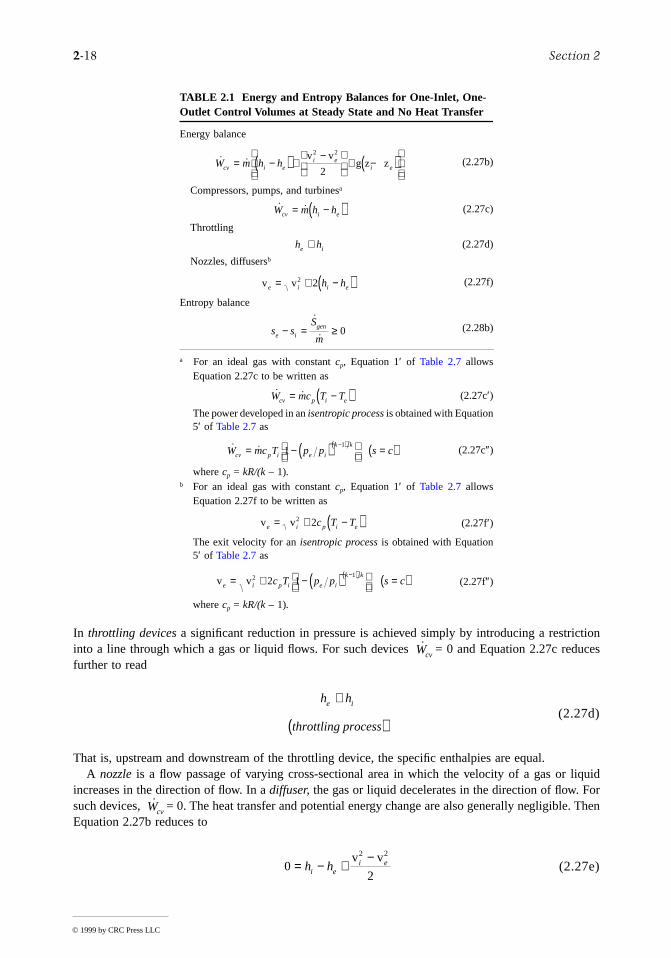
TABLE 2.1 Energy and Entropy Balances for One-Inlet, One-Outlet Control Volumes at Steady State and No Heat Transfer
Energy balance
(2.27b)
Compressors, pumps, and turbinesa
(2.27c)
Throttling
(2.27d)
Nozzles, diffusersb
(2.27f)
Entropy balance
(2.28b)
a For an ideal gas with constant cp, Equation 1′ of Table 2.7 allowsEquation 2.27c to be written as
(2.27c′)
The power developed in an isentropic process is obtained with Equation5′ of Table 2.7 as
(2.27c″)
where cp = kR/(k – 1).b For an ideal gas with constant cp, Equation 1′ of Table 2.7 allows
Equation 2.27f to be written as
(2.27f′)
The exit velocity for an isentropic process is obtained with Equation5′ of Table 2.7 as
(2.27f″)
where cp = kR/(k – 1).
˙ ˙W m h hcv i ei e
i e= −( ) +−
+ −( )
v vg z z
2 2
2
˙ ˙W m h hcv i e= −( )
h he i≅
v ve i i eh h= + −( )2 2
s sS
me igen− = ≥
˙
˙0
˙ ˙W mc T Tcv p i e= −( )
˙ ˙W mc T p p s ccv p i e i
k k= − ( )
=( )−( )1
1
v ve i p i ec T T= + −( )2 2
v ve i p i e i
k kc T p p s c= + − ( )
=( )−( )2 12 1
Wcv
h h
throttling process
e i≅
( )
Wcv
02
2 2
= − +−
h hi ei ev v
© 1999 by CRC Press LLC
Engineering Thermodynamics 2-19
n-
t
5%,
Solving for the outlet velocity
(2.27f)
Further discussion of the flow-through nozzles and diffusers is provided in Chapter 3.The mass, energy, and entropy rate balances, Equations 2.26, can be applied to control volumes with
multiple inlets and/or outlets, as, for example, cases involving heat-recovery steam generators, feedwaterheaters, and counterflow and crossflow heat exchangers. Transient (or unsteady) analyses can be coducted with Equations 2.19, 2.24, and 2.25. Illustrations of all such applications are provided by Moranand Shapiro (1995).
Example 1
A turbine receives steam at 7 MPa, 440°C and exhausts at 0.2 MPa for subsequent process heating duy.If heat transfer and kinetic/potential energy effects are negligible, determine the steam mass flow rate,in kg/hr, for a turbine power output of 30 MW when (a) the steam quality at the turbine outlet is 9(b) the turbine expansion is internally reversible.
Solution. With the indicated idealizations, Equation 2.27c is appropriate. Solving, Steam table data (Table A.5) at the inlet condition are hi = 3261.7 kJ/kg, si = 6.6022 kJ/kg · K.
(a) At 0.2 MPa and x = 0.95, he = 2596.5 kJ/kg. Then
(b) For an internally reversible expansion, Equation 2.28b reduces to give se = si. For this case, he =2499.6 kJ/kg (x = 0.906), and = 141,714 kg/hr.
Example 2
Air at 500°F, 150 lbf/in.2, and 10 ft/sec expands adiabatically through a nozzle and exits at 60°F, 15lbf/in.2. For a mass flow rate of 5 lb/sec determine the exit area, in in.2. Repeat for an isentropic expansionto 15 lbf/in.2. Model the air as an ideal gas (Section 2.3, Ideal Gas Model) with specific heat cp = 0.24Btu/lb · °R (k = 1.4).
Solution. The nozle exit area can be evaluated using Equation 2.20, together with the ideal gas equation,v = RT/p:
The exit velocity required by this expression is obtained using Equation 2.27f′ of Table 2.1,
v v
,
e i i eh h
nozzle diffuser
= + −( )( )
2 2
˙ ˙ /( ).m W h hcv i e= −
˙. .
sec
,
m =−( )
=
303261 7 2596 5
101
36001
162 357
3MWkJ kg
kJ secMW hr
kg hr
m
Am m RT p
ee
e
e e
e
= =( )˙ ˙ν
v v
v v
ft Btulb R
ft lbfBtu
Rlb ft seclbf
ft sec
2
e i p i ec T T
s
= + −( )
=
+
⋅
⋅
°( ) ⋅
=
2
2
2
102 0 24
778 171
44032 174
1
2299 5
.. .
.
© 1999 by CRC Press LLC
2-20 Section 2
Finally, with R = = 53.33 ft · lbf/lb · °R,
Using Equation 2.27f″ in Table 2.1 for the isentropic expansion,
Then Ae = 3.92 in.2.
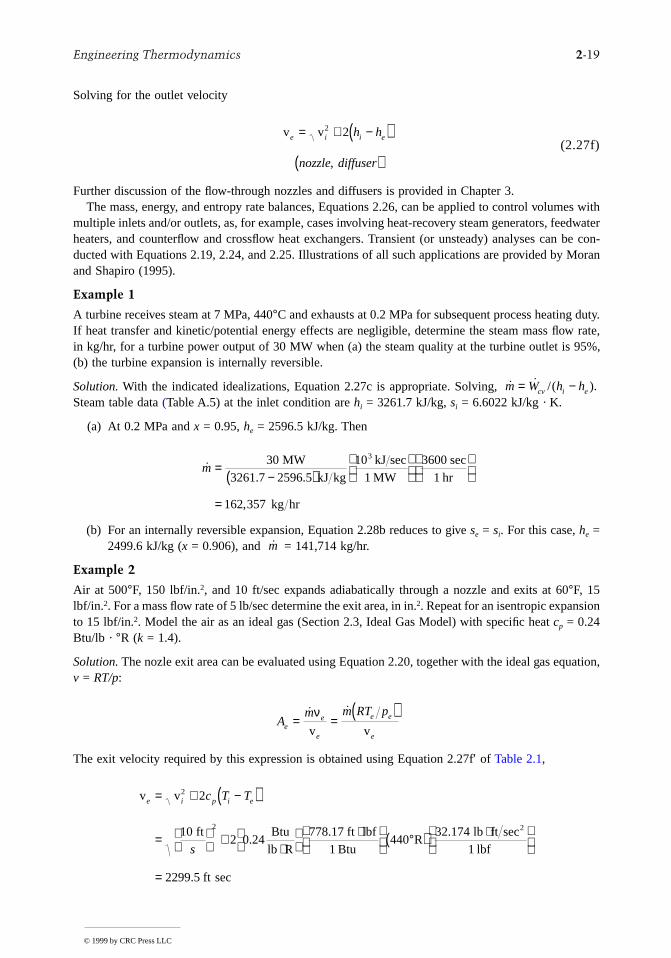
Example 3
Figure 2.2 provides steady-state operating data for an open feedwater heater. Ignoring heat transfer andkinetic/potential energy effects, determine the ratio of mass flow rates,
Solution. For this case Equations 2.26a and 2.26b reduce to read, respectively,
Combining and solving for the ratio
Inserting steam table data, in kJ/kg, from Table A.5,
Internally Reversible Heat Transfer and Work
For one-inlet, one-outlet control volumes at steady state, the following expressions give the heat transferrate and power in the absence of internal irreversibilities:
FIGURE 2.2 Open feedwater heater.
R /M
Ae =
⋅⋅ °
°( )
=5 53 3 520
2299 5 154 02
lb ft lbflb R
R
ft lbfin.
in.
2
2sec.
.sec
.
v
ft
e = ( ) + ( )( )( )( ) −
=
10 2 0 24 778 17 960 32 174 115
150
2358 3
20 4 1 4
. . .
. sec
. .
˙ / ˙ .m m1 2
˙ ˙ ˙
˙ ˙ ˙
m m m
m h m h m h
1 2 3
1 1 2 2 3 30
+ =
= + −
˙ / ˙ ,m m1 2
˙
˙m
m
h h
h h1
2
2 3
3 1
=−−
˙
˙. .. .
.m
m1
2
2844 8 697 2697 2 167 6
4 06= −−
=
© 1999 by CRC Press LLC
Engineering Thermodynamics 2-21
s
-c-d
(2.29)
(2.30a)
(see, e.g., Moran and Shapiro, 1995).If there is no significant change in kinetic or potential energy from inlet to outlet, Equation 2.30a read
(2.30b)
The specific volume remains approximately constant in many applications with liquids. Then Equation30b becomes
(2.30c)
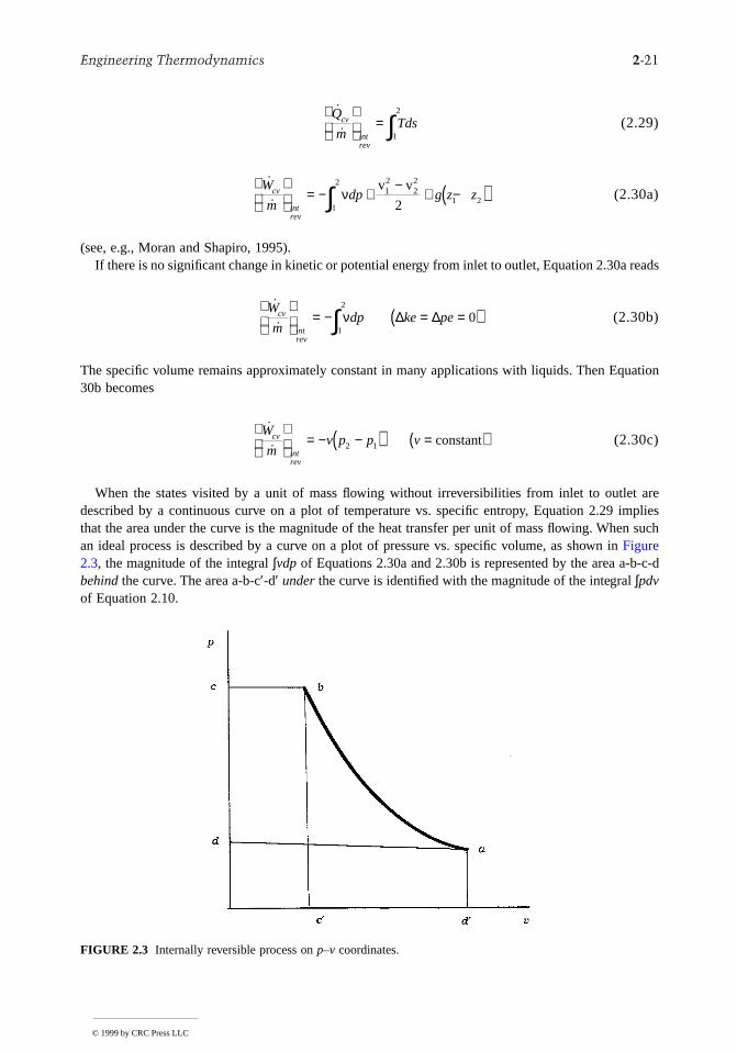
When the states visited by a unit of mass flowing without irreversibilities from inlet to outlet aredescribed by a continuous curve on a plot of temperature vs. specific entropy, Equation 2.29 impliesthat the area under the curve is the magnitude of the heat transfer per unit of mass flowing. When suchan ideal process is described by a curve on a plot of pressure vs. specific volume, as shown in Figure2.3, the magnitude of the integral ∫vdp of Equations 2.30a and 2.30b is represented by the area a-bbehind the curve. The area a-b-c′-d′ under the curve is identified with the magnitude of the integral ∫pdvof Equation 2.10.
FIGURE 2.3 Internally reversible process on p–v coordinates.
˙
˙Q
mTdscv
rev
= ∫int 1
2
˙
˙W
mdp g z zcv
rev
= − +
−+ −( )∫int
νv v1
222
1
2
1 22
˙
˙W
mdp ke pecv
rev
= − = =( )∫int
ν ∆ ∆ 01
2
˙
˙W
mv p p vcv
rev
= − −( ) =( )
int2 1 constant
© 1999 by CRC Press LLC
2-22 Section 2
een thelly, asoperties usingropriates and
y
g
ences variousell.
rocess
:olume
2.3 Property Relations and Data
Pressure, temperature, volume, and mass can be found experimentally. The relationships betwspecific heats cv and cp and temperature at relatively low pressure are also accessible experimentaare certain other property data. Specific internal energy, enthalpy, and entropy are among those prthat are not so readily obtained in the laboratory. Values for such properties are calculatedexperimental data of properties that are more amenable to measurement, together with appproperty relations derived using the principles of thermodynamics. In this section property relationdata sources are considered for simple compressible systems, which include a wide range of industriallyimportant substances.
Property data are provided in the publications of the National Institute of Standards and Technolog(formerly the U.S. Bureau of Standards), of professional groups such as the American Society ofMechanical Engineering (ASME), the American Society of Heating. Refrigerating, and Air ConditioninEngineers (ASHRAE), and the American Chemical Society, and of corporate entities such as Dupont andDow Chemical. Handbooks and property reference volumes such as included in the list of referfor this chapter are readily accessed sources of data. Property data are also retrievable fromcommercial online data bases. Computer software is increasingly available for this purpose as w
Basic Relations for Pure Substances
An energy balance in differential form for a closed system undergoing an internally reversible pin the absence of overall system motion and the effect of gravity reads
From Equation 2.14b, = TdS. When consideration is limited to simple compressible systemssystems for which the only significant work in an internally reversible process is associated with vchange, = pdV, the following equation is obtained:
(2.31a)
Introducing enthalpy, H = U + pV, the Helmholtz function, Ψ = U – TS, and the Gibbs function, G = H– TS, three additional expressions are obtained:
(2.31b)
(2.31c)
(2.31d)
Equations 2.31 can be expressed on a per-unit-mass basis as
(2.32a)
(2.32b)
(2.32c)
(2.32d)
dU Q Wrev rev
= ( ) − ( )δ δint int
δQrev( )int
δWrev( )int
dU TdS pdV= −
dH TdS Vdp= +
d pdV SdTΨ = − −
dG Vdp SdT= −
du Tds pdv= −
dh Tds vdp= +
d pdv sdTψ = − −
dg vdp sdT= −
© 1999 by CRC Press LLC
Engineering Thermodynamics 2-23
ly,
Similar expressions can be written on a per-mole basis.
Maxwell Relations
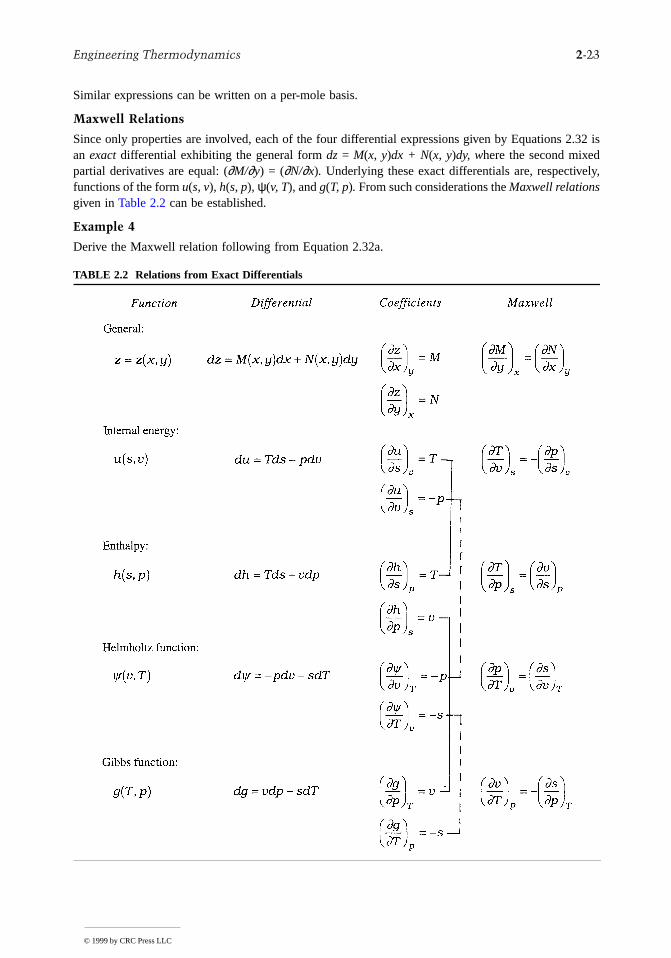
Since only properties are involved, each of the four differential expressions given by Equations 2.32 isan exact differential exhibiting the general form dz = M(x, y)dx + N(x, y)dy, where the second mixedpartial derivatives are equal: (∂M/∂y) = (∂N/∂x). Underlying these exact differentials are, respectivefunctions of the form u(s, v), h(s, p), ψ(v, T), and g(T, p). From such considerations the Maxwell relationsgiven in Table 2.2 can be established.
Example 4
Derive the Maxwell relation following from Equation 2.32a.
TABLE 2.2 Relations from Exact Differentials
© 1999 by CRC Press LLC
2-24 Section 2
e
among
Solution. The differential of the function u = u(s, v) is
By comparison with Equation 2.32a,
In Equation 2.32a, T plays the role of M and –p plays the role of N, so the equality of second mixedpartial derivatives gives the Maxwell relation,
Since each of the properties T, p, v, and s appears on the right side of two of the eight coefficients ofTable 2.2, four additional property relations can be obtained by equating such expressions:
These four relations are identified in Table 2.2 by brackets. As any three of Equations 2.32 can bobtained from the fourth simply by manipulation, the 16 property relations of Table 2.2 also can beregarded as following from this single differential expression. Several additional first-derivative propertyrelations can be derived; see, e.g., Zemansky, 1972.
Specific Heats and Other Properties
Engineering thermodynamics uses a wide assortment of thermodynamic properties and relationsthese properties. Table 2.3 lists several commonly encountered properties.
Among the entries of Table 2.3 are the specific heats cv and cp. These intensive properties are oftenrequired for thermodynamic analysis, and are defined as partial derivations of the functions u(T, v) andh(T, p), respectively,
(2.33)
(2.34)
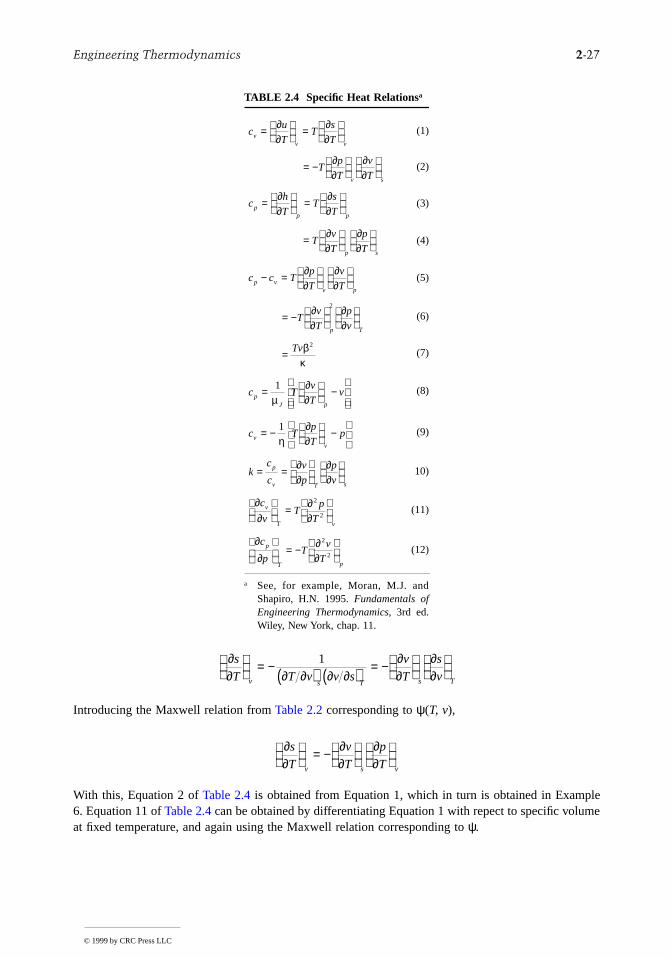
Since u and h can be expressed either on a unit mass basis or a per-mole basis, values of the specificheats can be similarly expressed. Table 2.4 summarizes relations involving cv and cp. The property k,the specific heat ratio, is
(2.35)
duu
sds
u
vdv
v s
=
+
∂∂
∂∂
Tu
sp
u
vv s
=
− =
∂∂
∂∂
,
∂∂
∂∂
T
v
p
ss v
= −
∂∂
∂∂
∂∂
∂ψ∂
∂∂
∂∂
∂ψ∂
∂∂
u
s
h
s
u
v v
h
p
g
p T
g
T
v p s T
s T v p
=
=
=
=
,
,
cu
Tvv
=
∂∂
ch
Tpp
=
∂∂
kc
cp
v
=
© 1999 by CRC Press LLC
Engineering Thermodynamics 2-25
the
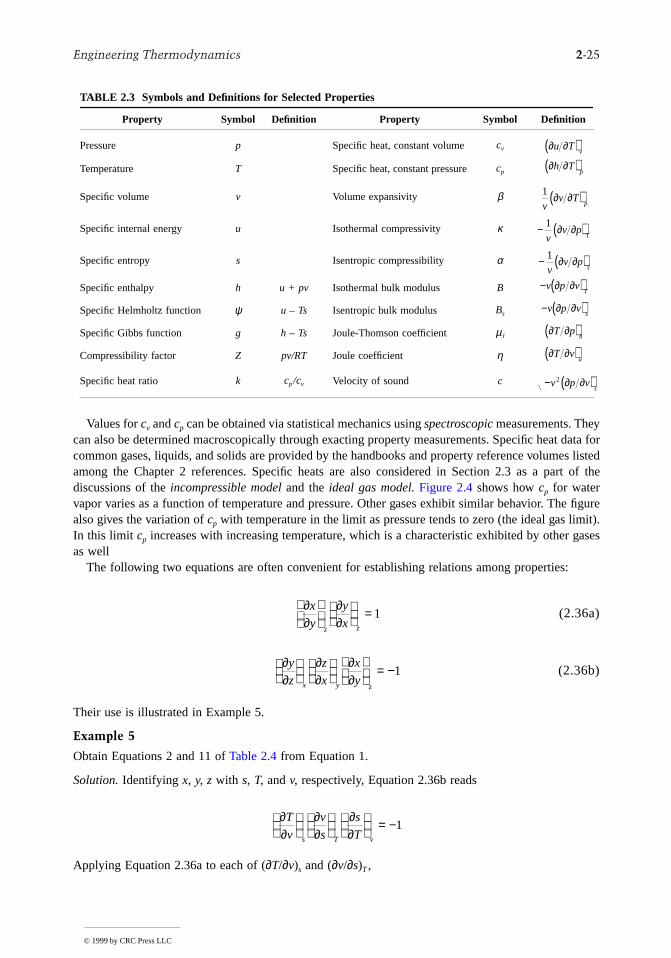
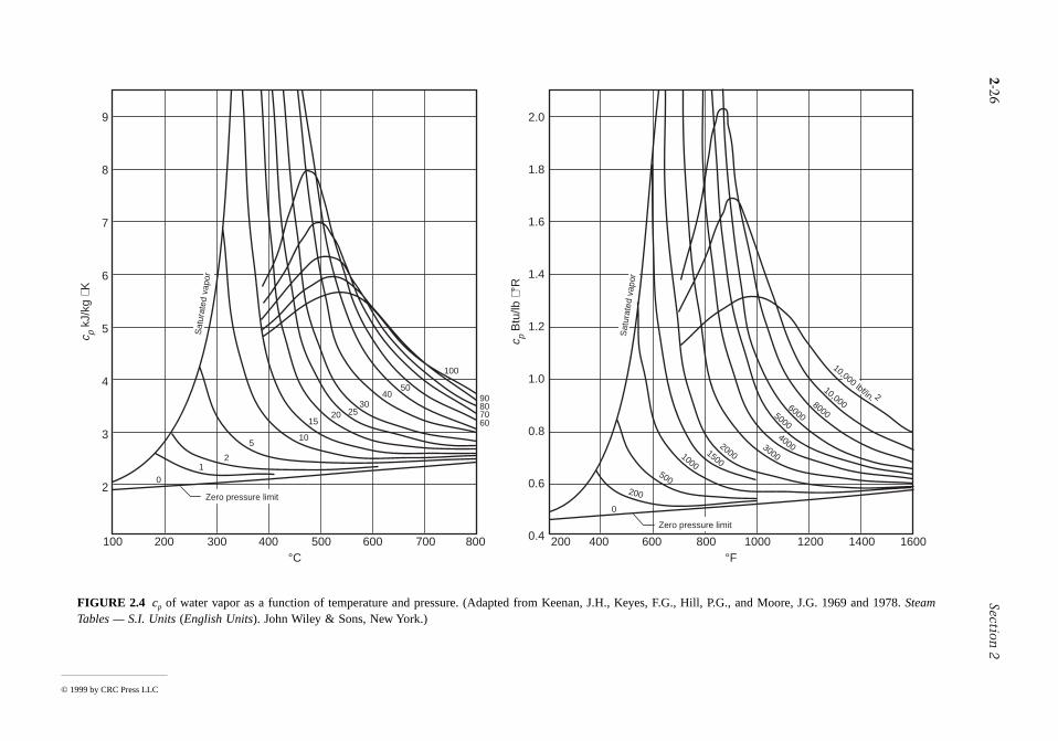
Values for cv and cp can be obtained via statistical mechanics using spectroscopic measurements. Theycan also be determined macroscopically through exacting property measurements. Specific heat data forcommon gases, liquids, and solids are provided by the handbooks and property reference volumes listedamong the Chapter 2 references. Specific heats are also considered in Section 2.3 as a part ofdiscussions of the incompressible model and the ideal gas model. Figure 2.4 shows how cp for watervapor varies as a function of temperature and pressure. Other gases exhibit similar behavior. The figurealso gives the variation of cp with temperature in the limit as pressure tends to zero (the ideal gas limit).In this limit cp increases with increasing temperature, which is a characteristic exhibited by other gasesas well
The following two equations are often convenient for establishing relations among properties:
(2.36a)
(2.36b)
Their use is illustrated in Example 5.
Example 5
Obtain Equations 2 and 11 of Table 2.4 from Equation 1.
Solution. Identifying x, y, z with s, T, and v, respectively, Equation 2.36b reads
Applying Equation 2.36a to each of (∂T/∂v)s and (∂v/∂s)T,
TABLE 2.3 Symbols and Definitions for Selected Properties
Property Symbol Definition Property Symbol Definition
Pressure p Specific heat, constant volume cv
Temperature T Specific heat, constant pressure cp
Specific volume v Volume expansivity β
Specific internal energy u Isothermal compressivity κ
Specific entropy s Isentropic compressibility α
Specific enthalpy h u + pv Isothermal bulk modulus B
Specific Helmholtz function ψ u – Ts Isentropic bulk modulus Bs
Specific Gibbs function g h – Ts Joule-Thomson coefficient µJ
Compressibility factor Z pv/RT Joule coefficient η
Specific heat ratio k cp/cv Velocity of sound c
∂ ∂u Tv( )
∂ ∂h Tp( )
1
vv T
p∂ ∂( )
− ( )1
vv p
T∂ ∂
− ( )1
vv p
s∂ ∂
− ( )v p vT
∂ ∂
− ( )v p vs
∂ ∂
∂ ∂T ph( )
∂ ∂T vu( )
− ( )v p vs
2 ∂ ∂
∂∂
∂∂
x
y
y
xz z
= 1
∂∂
∂∂
∂∂
y
z
z
x
x
yx y z
= −1
∂∂
∂∂
∂∂
T
v
v
s
s
Ts T v
= −1
© 1999 by CRC Press LLC
2-26Section
2
© 19
F eyes, F.G., Hill, P.G., and Moore, J.G. 1969 and 1978. SteamT
800°F
1000 1200 1400 1600
ero pressure limit
0
1000
1500
20003000
4000
5000
60008000
10,000
10,000 lbf/in. 2
99 by CRC Press LLC
IGURE 2.4 cp of water vapor as a function of temperature and pressure. (Adapted from Keenan, J.H., Kables — S.I. Units (English Units). John Wiley & Sons, New York.)
100 200 300 400 500 600 700 800°C
9
8
7
6
5
4
3
2
c p kJ
/kg
⋅ K
Zero pressure limit
Sat
urat
ed v
apor
200 400 600
2.0
1.8
1.6
1.4
1.2
1.0
0.8
0.6
0.4
c p B
tu/lb
⋅ °R
Z
Sat
urat
ed v
apor
0
200
500
12
510
1520 25
3040
50
60708090
100
Engineering Thermodynamics 2-27
le
Introducing the Maxwell relation from Table 2.2 corresponding to ψ(T, v),
With this, Equation 2 of Table 2.4 is obtained from Equation 1, which in turn is obtained in Examp6. Equation 11 of Table 2.4 can be obtained by differentiating Equation 1 with repect to specific volumeat fixed temperature, and again using the Maxwell relation corresponding to ψ.
TABLE 2.4 Specific Heat Relationsa
(1)
(2)
(3)
(4)
(5)
(6)
(7)
(8)
(9)
10)
(11)
(12)
a See, for example, Moran, M.J. andShapiro, H.N. 1995. Fundamentals ofEngineering Thermodynamics, 3rd ed.Wiley, New York, chap. 11.
cu
TT
s
Tvv v
=
=
∂∂
∂∂
= −
Tp
T
v
Tv s
∂∂
∂∂
ch
TT
s
Tpp p
=
=
∂∂
∂∂
=
Tv
T
p
Tp s
∂∂
∂∂
c c Tp
T
v
Tp vv p
− =
∂∂
∂∂
= −
Tv
T
p
vp T
∂∂
∂∂
2
= Tvβκ
2
c Tv
Tvp
J p
=
−
1
µ∂∂
c Tp
Tpv
v
= −
−
1
η∂∂
kc
c
v
p
p
vp
v T s
= =
∂∂
∂∂
∂∂
∂∂
c
vT
p
Tv
T v
=
2
2
∂∂
∂∂
c
pT
v
Tp
T p
= −
2
2
∂∂ ∂ ∂ ∂ ∂
∂∂
∂∂
s
T T v v s
v
T
s
vv s T s T
= − ( ) ( ) = −
1
∂∂
∂∂
∂∂
s
T
v
T
p
Tv s v
= −
© 1999 by CRC Press LLC
2-28 Section 2
re
d
P-v-T Relations
Considerable pressure, specific volume, and temperature data have been accumulated for industriallyimportant gases and liquids. These data can be represented in the form p = f (v, T ), called an equationof state. Equations of state can be expressed in tabular, graphical, and analytical forms.
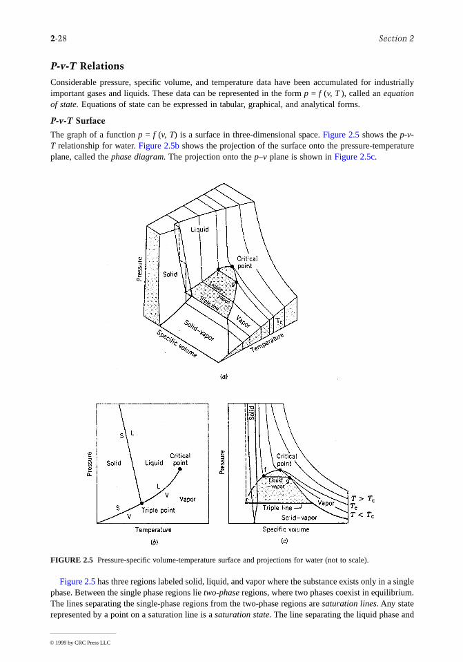
P-v-T Surface
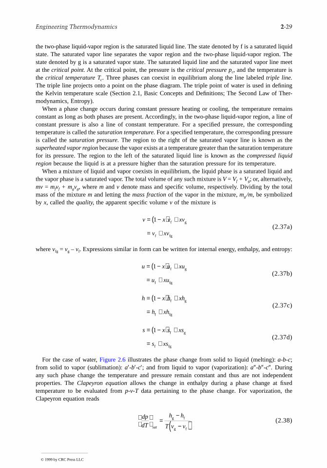
The graph of a function p = f (v, T) is a surface in three-dimensional space. Figure 2.5 shows the p-v-T relationship for water. Figure 2.5b shows the projection of the surface onto the pressure-temperatuplane, called the phase diagram. The projection onto the p–v plane is shown in Figure 2.5c.
Figure 2.5 has three regions labeled solid, liquid, and vapor where the substance exists only in a singlephase. Between the single phase regions lie two-phase regions, where two phases coexist in equilibrium.The lines separating the single-phase regions from the two-phase regions are saturation lines. Any staterepresented by a point on a saturation line is a saturation state. The line separating the liquid phase an
FIGURE 2.5 Pressure-specific volume-temperature surface and projections for water (not to scale).
© 1999 by CRC Press LLC
Engineering Thermodynamics 2-29
id
remains
ngure
ture
.nd
ependent
the two-phase liquid-vapor region is the saturated liquid line. The state denoted by f is a saturated liqustate. The saturated vapor line separates the vapor region and the two-phase liquid-vapor region. Thestate denoted by g is a saturated vapor state. The saturated liquid line and the saturated vapor line meetat the critical point. At the critical point, the pressure is the critical pressure pc, and the temperature isthe critical temperature Tc. Three phases can coexist in equilibrium along the line labeled triple line.The triple line projects onto a point on the phase diagram. The triple point of water is used in definingthe Kelvin temperature scale (Section 2.1, Basic Concepts and Definitions; The Second Law of Ther-modynamics, Entropy).
When a phase change occurs during constant pressure heating or cooling, the temperatureconstant as long as both phases are present. Accordingly, in the two-phase liquid-vapor region, a line ofconstant pressure is also a line of constant temperature. For a specified pressure, the corresponditemperature is called the saturation temperature. For a specified temperature, the corresponding pressis called the saturation pressure. The region to the right of the saturated vapor line is known as thesuperheated vapor region because the vapor exists at a temperature greater than the saturation temperafor its pressure. The region to the left of the saturated liquid line is known as the compressed liquidregion because the liquid is at a pressure higher than the saturation pressure for its temperature
When a mixture of liquid and vapor coexists in equilibrium, the liquid phase is a saturated liquid athe vapor phase is a saturated vapor. The total volume of any such mixture is V = Vf + Vg; or, alternatively,mv = mfvf + mgvg, where m and v denote mass and specific volume, respectively. Dividing by the totalmass of the mixture m and letting the mass fraction of the vapor in the mixture, mg/m, be symbolizedby x, called the quality, the apparent specific volume v of the mixture is
(2.37a)
where vfg = vg – vf. Expressions similar in form can be written for internal energy, enthalpy, and entropy:
(2.37b)
(2.37c)
(2.37d)
For the case of water, Figure 2.6 illustrates the phase change from solid to liquid (melting): a-b-c;from solid to vapor (sublimation): a′-b′-c′; and from liquid to vapor (vaporization): a″-b″-c″. Duringany such phase change the temperature and pressure remain constant and thus are not indproperties. The Clapeyron equation allows the change in enthalpy during a phase change at fixedtemperature to be evaluated from p-v-T data pertaining to the phase change. For vaporization, theClapeyron equation reads
(2.38)
v x v xv
v xv
= −( ) +
= +
1 f g
f fg
u x u xu
u xu
= −( ) +
= +
1 f g
f fg
h x h xh
h xh
= −( ) +
= +
1 f g
f fg
s x s xs
s xs
= −( ) +
= +
1 f g
f fg
dp
dT
h h
T v vsat
=
−
−( )g f
g f
© 1999 by CRC Press LLC
2-30 Section 2
.38 can
n theen
d
ity
where (dp/dT)sat is the slope of the saturation pressure-temperature curve at the point determined by thetemperature held constant during the phase change. Expressions similar in form to Equation 2be written for sublimation and melting.
The Clapeyron equation shows that the slope of a saturation line on a phase diagram depends osigns of the specific volume and enthalpy changes accompanying the phase change. In most cases, wha phase change takes place with an increase in specific enthalpy, the specific volume also increases, and(dp/dT)sat is positive. However, in the case of the melting of ice and a few other substances, the specificvolume decreases on melting. The slope of the saturated solid-liquid curve for these few substances isnegative, as illustrated for water in Figure 2.6.
Graphical Representations
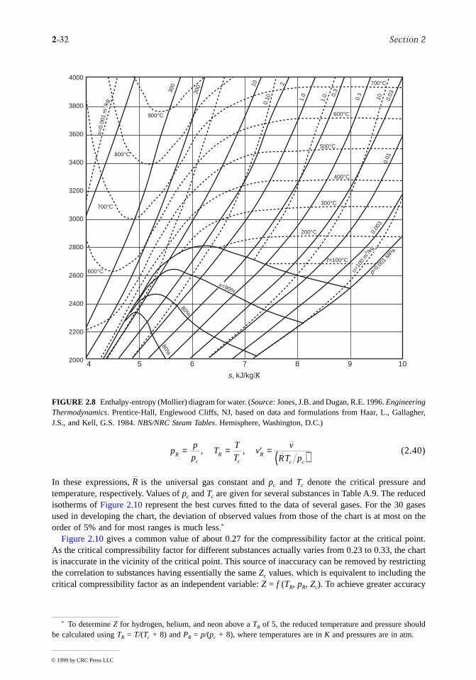
The intensive states of a pure, simple compressible system can be represented graphically with any twoindependent intensive properties as the coordinates, excluding properties associated with motion angravity. While any such pair may be used, there are several selections that are conventionally employed.These include the p-T and p-v diagrams of Figure 2.5, the T-s diagram of Figure 2.7, the h-s (Mollier)diagram of Figure 2.8, and the p-h diagram of Figure 2.9. The compressibility charts considered nextuse the compressibility factor as one of the coordinates.
Compressibility Charts
The p-v-T relation for a wide range of common gases is illustrated by the generalized compressibilchart of Figure 2.10. In this chart, the compressibility factor, Z, is plotted vs. the reduced pressure, pR,reduced temperature, TR, and pseudoreduced specific volume, where
(2.39)
and
FIGURE 2.6 Phase diagram for water (not to scale).
′vR ,
Zpv
RT=
© 1999 by CRC Press LLC
En
gineerin
g Th
ermod
ynam
ics2-31
©
ering Thermodynamics, Prentice-Hall,.S. 1984. NBS/NRC Steam Tables. Hemisphere,
9 10
0.1
0.03
100.
01
0.00
3
p=0.
001
MPa
υ=10
0 m
3 /kg
C
°C
C
700°C
1999 by CRC Press LLC
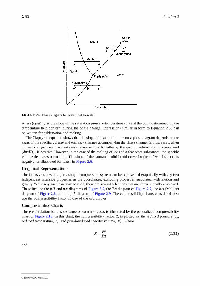
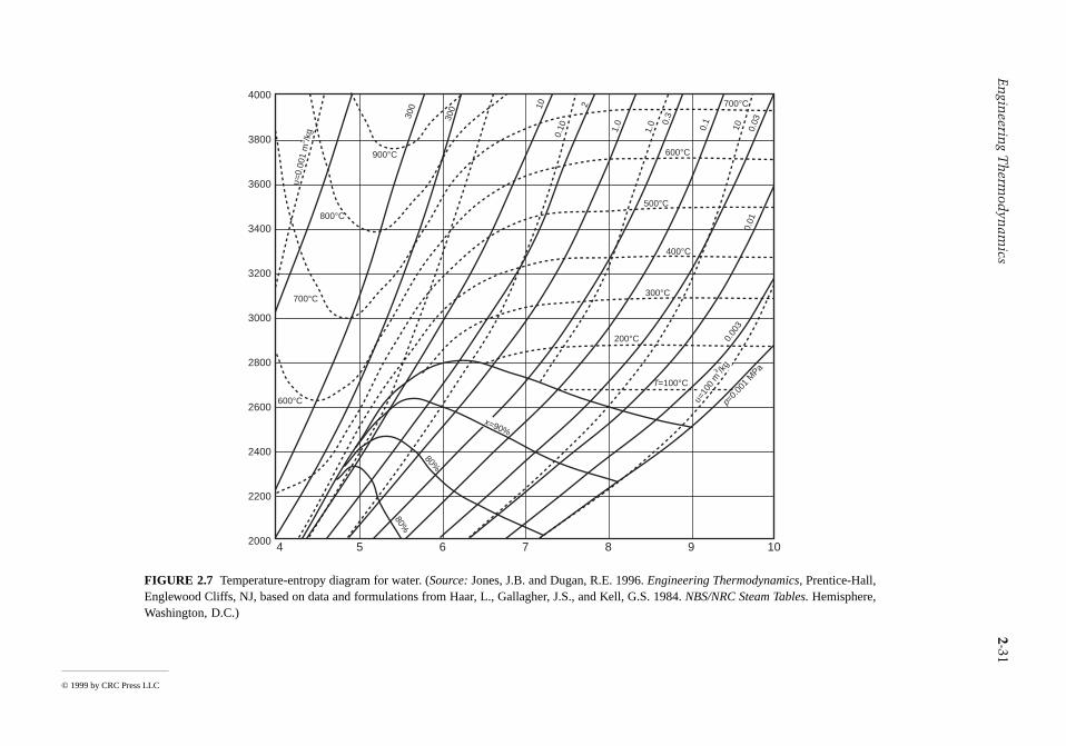
FIGURE 2.7 Temperature-entropy diagram for water. (Source: Jones, J.B. and Dugan, R.E. 1996. EngineEnglewood Cliffs, NJ, based on data and formulations from Haar, L., Gallagher, J.S., and Kell, GWashington, D.C.)
4
4000
3800
3600
3400
3200
3000
2800
2600
2400
2200
2000 5 6 7 8
900°C
800°C
700°C
600°C
υ=0.
001
m3 /k
g
300
300 10
0.10
2
1.0
1.0 0.
3
80%
80%
x=90%
T=100°
200°C
300°C
400
500°C
600°
2-32 Section 2
d
he
t
uld
(2.40)
In these expressions, is the universal gas constant and pc and Tc denote the critical pressure antemperature, respectively. Values of pc and Tc are given for several substances in Table A.9. The reducedisotherms of Figure 2.10 represent the best curves fitted to the data of several gases. For the 30 gasesused in developing the chart, the deviation of observed values from those of the chart is at most on torder of 5% and for most ranges is much less.*
Figure 2.10 gives a common value of about 0.27 for the compressibility factor at the critical point.As the critical compressibility factor for different substances actually varies from 0.23 to 0.33, the charis inaccurate in the vicinity of the critical point. This source of inaccuracy can be removed by restrictingthe correlation to substances having essentially the same Zc values. which is equivalent to including thecritical compressibility factor as an independent variable: Z = f (TR, pR, Zc). To achieve greater accuracy
* To determine Z for hydrogen, helium, and neon above a TR of 5, the reduced temperature and pressure shobe calculated using TR = T/(Tc + 8) and PR = p/(pc + 8), where temperatures are in K and pressures are in atm.
FIGURE 2.8 Enthalpy-entropy (Mollier) diagram for water. (Source: Jones, J.B. and Dugan, R.E. 1996. EngineeringThermodynamics. Prentice-Hall, Englewood Cliffs, NJ, based on data and formulations from Haar, L., Gallagher,J.S., and Kell, G.S. 1984. NBS/NRC Steam Tables. Hemisphere, Washington, D.C.)
4
4000
3800
3600
3400
3200
3000
2800
2600
2400
2200
2000 5 6 7 8 9 10
s, kJ/kg⋅K
900°C
800°C
700°C
600°C
υ=0.
001
m3 /k
g
300
300 10
0.10
2
1.0
1.0 0.
3
0.1
0.03
100.
01
0.00
3
p=0.
001
MPa
υ=10
0 m
3 /kg
80%
80%
x=90%
T=100°C
200°C
300°C
400°C
500°C
600°C
700°C
pp
pT
T
Tv
v
RT pRc
Rc
Rc c
= = ′ = ( ), ,
R
© 1999 by CRC Press LLC
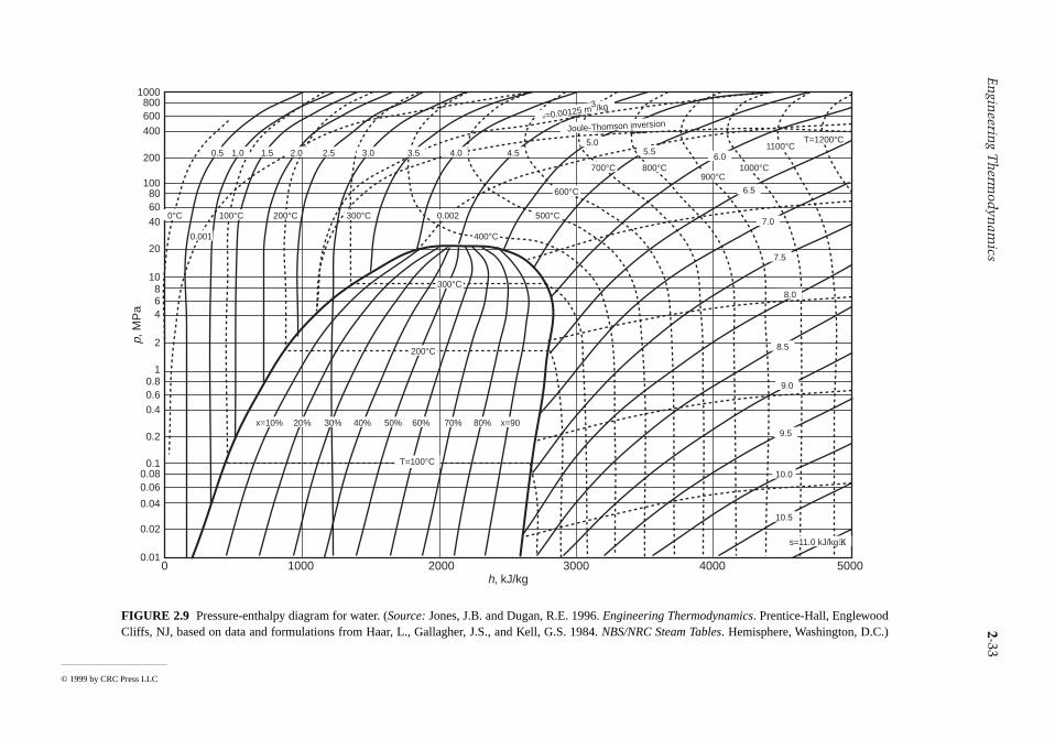
En
gineerin
g Th
ermod
ynam
ics2-33
©
hermodynamics. Prentice-Hall, Englewoodeam Tables. Hemisphere, Washington, D.C.)
4000 5000
10.5
10.0
9.5
9.0
8.5
8.0
7.5
7.0
6.5
6.0
900°C1000°C
1100°CT=1200°C
s=11.0 kJ/kg⋅K
1999 by CRC Press LLC
FIGURE 2.9 Pressure-enthalpy diagram for water. (Source: Jones, J.B. and Dugan, R.E. 1996. Engineering TCliffs, NJ, based on data and formulations from Haar, L., Gallagher, J.S., and Kell, G.S. 1984. NBS/NRC St
0.01
h, kJ/kg10000 2000 3000
p, M
Pa
0.02
0.04
0.060.08
0.1
0.2
0.40.60.8
1
10864
2
20
406080
100
200
400600800
1000
x=10% 20% 30% 40% 50% 60% 70% 80% x=90
5.55.0
4.54.03.53.02.52.01.51.00.5
0°C
0.001
100°C 200°C 300°C 0.002
400°C
500°C
600°C
700°C 800°C
300°C
200°C
0°C
T=100°C
Joule-Thomson inversionν=0.00125 m
3/kg
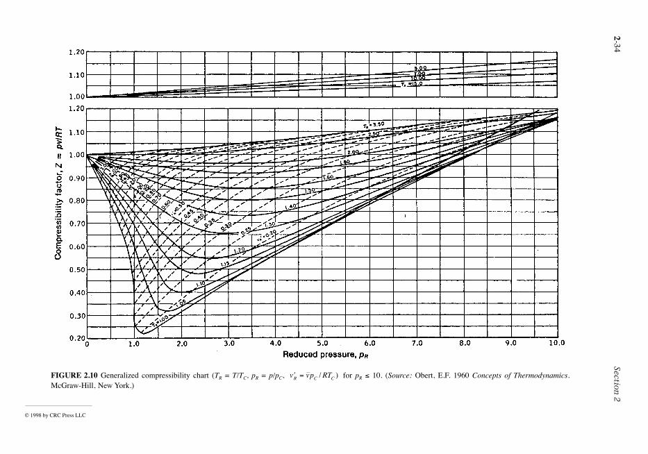
2
-34
Section 2
© 1998 b
bert, E.F. 1960
Concepts of Thermodynamics
.
y CRC Press LLC
FIGURE 2.10 Generalized compressibility chart (TR = T/TC, pR = p/pC, for pR £ 10. (Source: OMcGraw-Hill, New York.)
¢ =v vp RTR C C/ )
Engineering Thermodynamics 2-35
d as a
.
ns
by
from
variables other than
Z
c
have been proposed as a third parameter — for example, the
acentric factor
(see,e.g., Reid and Sherwood, 1966).
Generalized compressibility data are also available in tabular form (see, e.g., Reid and Sherwood,1966) and in equation form (see, e.g., Reynolds, 1979). The use of generalized data in any form (graphical,tabular, or equation) allows
p
,
v
, and
T
for gases to be evaluated simply and with reasonable accuracy.When accuracy is an essential consideration, generalized compressibility data should not be usesubstitute for
p-v-T
data for a given substance as provided by computer software, a table, or an equationof state.
Equations of State
Considering the isotherms of Figure 2.10, it is plausible that the variation of the compressibility factormight be expressed as an equation, at least for certain intervals of
p
and
T
. Two expressions can bewritten that enjoy a theoretical basis. One gives the compressibility factor as an infinite series expansionin pressure,
and the other is a series in
These expressions are known as
virial expansions
,
and the coefficients …
and
B
,
C
,
D
… arecalled
virial coefficients.
In principle, the virial coefficients can be calculated using expressions fromstatistical mechanics derived from consideration of the force fields around the molecules. Thus far onlythe first few coefficients have been calculated and only for gases consisting of relatively simple molecules.The coefficients also can be found, in principle, by fitting
p-v-T
data in particular realms of interestOnly the first few coefficients can be found accurately this way, however, and the result is a
truncated
equation valid only at certain states.Over 100 equations of state have been developed in an attempt to portray accurately the
p-v-T
behaviorof substances and yet avoid the complexities inherent in a full virial series. In general, these equatioexhibit little in the way of fundamental physical significance and are mainly empirical in character. Mostare developed for gases, but some describe the
p-v-T
behavior of the liquid phase, at least qualitatively.Every equation of state is restricted to particular states. The realm of applicability is often indicated bygiving an interval of pressure, or density, where the equation can be expected to represent the
p-v-T
behavior faithfully. When it is not stated, the realm of applicability often may be approximatedexpressing the equation in terms of the compressibility factor
Z
and the reduced properties, and super-imposing the result on a generalized compressibility chart or comparing with compressibility datathe literature.
Equations of state can be classified by the number of adjustable constants they involve. The Redlich-Kwong equation is considered by many to be the best of the two-constant equations of state. It givespressure as a function of temperature and specific volume and thus is
explicit
in pressure:
(2.41)
This equation is primarily empirical in nature, with no rigorous justification in terms of moleculararguments. Values for the Redlich-Kwong constants for several substances are provided in Table A.9.Modified forms of the equation have been proposed with the aim of achieving better accuracy.
Z B T p C T p D T p= + ( ) + ( ) + ( ) +1 2 3ˆ ˆ ˆ K
1/ ,v
Z
B T
v
C T
v
D T
v= + ( ) + ( ) + ( ) +1 2 3 K
ˆ, ˆ ˆ ,B C D
pRT
v b
a
v v b T=
−−
+( ) 1 2
© 1999 by CRC Press LLC
2-36 Section 2
f stateressurenstants.s been
e, e.g., 12
d in ther more
aryingh as air.icting
ciples.operty
iscussedects of
uallar
verall
Although the two-constant Redlich-Kwong equation performs better than some equations ohaving several adjustable constants, two-constant equations tend to be limited in accuracy as p(or density) increases. Increased accuracy normally requires a greater number of adjustable coFor example, the Benedict-Webb-Rubin equation, which involves eight adjustable constants, hasuccessful in predicting the
p-v-T
behavior of
light hydrocarbons.
The Benedict-Webb-Rubin equationis also explicit in pressure,
(2.42)
Values of the Benedict-Webb-Rubin constants for various gases are provided in the literature (seCooper and Goldfrank, 1967). A modification of the Benedict-Webb-Rubin equation involvingconstants is discussed by Lee and Kessler, 1975. Many multiconstant equations can be founengineering literature, and with the advent of high speed computers, equations having 50 oconstants have been developed for representing the
p-v-T
behavior of different substances.
Gas Mixtures
Since an unlimited variety of mixtures can be formed from a given set of pure components by vthe relative amounts present, the properties of mixtures are reported only in special cases sucMeans are available for predicting the properties of mixtures, however. Most techniques for predmixture properties are empirical in character and are not derived from fundamental physical prinThe realm of validity of any particular technique can be established by comparing predicted prvalues with empirical data. In this section, methods for evaluating the
p-v-T
relations for pure componentsare adapted to obtain plausible estimates for gas mixtures. The case of ideal gas mixtures is din Section 2.3, Ideal Gas Model. In Section 2.3, Multicomponent Systems, some general aspproperty evaluation for multicomponent systems are presented.
The total number of moles of mixture,
n
,
is
the sum of the number of moles of the components,
n
i
:
(2.43)
The
relative
amounts of the components present can be described in terms of
mole fractions.
The molefraction
y
i
of component
i
is
y
i
=
n
i
/n.
The sum of the mole fractions of all components present is eqto unity. The apparent molecular weight
M
is the mole fraction average of the component molecuweights, such that
(2.44)
The
relative
amounts of the components present also can be described in terms of
mass fractions: m
i
/m,
where
m
i
is the mass of component
i
and
m
is the total mass of mixture.The
p-v-T
relation for a gas mixture can be estimated by applying an equation of state to the omixture. The constants appearing in the equation of state are
mixture values
determined with empiricalcombining rules developed for the equation. For example, mixture values of the constants
a
and
b
foruse in the Redlich-Kwong equation are obtained using relations of the form
(2.45)
pRT
vBRT A
C
T v
bRT a
v
a
v
c
v T v v= + − −
+
−( )+ + +
−
2 2 3 6 3 2 2 2
11
α γ γexp
n n n n nj i
i
j
= + + ==
∑1 2
1
K
M M==
∑ yi i
i
j
1
a y a b y bi i
i
j
i i
i
j
=
=
= =∑ ∑1 2
1
2
1
,
© 1999 by CRC Press LLC
Engineering Thermodynamics 2-37
g
where
a
i
and
b
i
are the values of the constants for component
i
. Combination rules for obtaining mixturevalues for the constants in other equations of state are also found in the literature.
Another approach is to regard the mixture as if it were a single pure component having criticalproperties calculated by one of several mixture rules.
Kay
’
s rule is
perhaps the simplest of these, requirinonly the determination of a mole fraction averaged critical temperature
T
c
and critical pressure
p
c
:
(2.46)
where
T
c,i
and
p
c,i
are the critical temperature and critical pressure of component
i
, respectively. Using
T
c
and
p
c
, the mixture compressibility factor Z is obtained as for a single pure component. The unkownquantity from among the pressure p, volume V, temperature T, and total number of moles n of the gasmixture can then be obtained by solving Z = pV/n T.
Additional means for predicting the p-v-T relation of a mixture are provided by empirical mixturerules. Several are found in the engineering literature. According to the additive pressure rule, the pressureof a gas mixture is expressible as a sum of pressures exerted by the individual components:
(2.47a)
where the pressures p1 , p2 , etc. are evaluated by considering the respective components to be at thevolume V and temperature T of the mixture. The additive pressure rule can be expressed alternatively as
(2.47b)
where Z is the compressibility factor of the mixture and the compressibility factors Zi are determinedassuming that component i occupies the entire volume of the mixture at the temperature T.
The additive volume rule postulates that the volume V of a gas mixture is expressible as the sum ofvolumes occupied by the individual components:
(2.48a)
where the volumes V1, V2, etc. are evaluated by considering the respective components to be at thepressure p and temperature T of the mixture. The additive volume rule can be expressed alternatively as
(2.48b)
where the compressibility factors Zi are determined assuming that component i exists at the pressure pand temperature T of the mixture.
Evaluating ∆h, ∆u, and ∆s
Using appropriate specific heat and p-v-T data, the changes in specific enthalpy, internal energy, andentropy can be determined between states of single-phase regions. Table 2.5 provides expressions forsuch property changes in terms of particular choices of the independent variables: temperature andpressure, and temperature and specific volume.
T y T p y pc i c i
i
j
c i c i
i
j
= == =
∑ ∑, ,,1 1
R
p p p p
T V= + + ]1 2 3K ,
Z y Zi i
i
j
T V
=
=
∑1 ,
V V V V
p T= + + ]1 2 3K ,
Z y Zi i
i
j
p T
=
=
∑1 ,
© 1999 by CRC Press LLC
2-38 Section 2
r
t
Taking Equation 1 of Table 2.5 as a representative case, the change in specific enthalpy between states1 and 2 can be determined using the three steps shown in the accompanying property diagram. Thisrequires knowledge of the variation of cp with temperature at a fixed pressure p′, and the variation of [v– T(∂v/∂T)p] with pressure at temperatures T1 and T2:
1-a: Since temperature is constant at T1, the first integral of Equation 1 in Table 2.5 vanishes, and
a-b: Since pressure is constant at p′, the second integral of Equation 1 vanishes, and
b-2: Since temperature is constant at T2, the first integral of Equation 1 vanishes, and
Adding these expressions, the result is h2 – h1. The required integrals may be performed numerically oanalytically. The analytical approach is expedited when an equation of state explicit in specific volumeis known.
Similar considerations apply to Equations 2 to 4 of Table 2.5. To evaluate u2 – u1 with Equation 3,for example, requires the variation of cv with temperature at a fixed specific volume v′, and the variationof [T(∂p/∂T)v – p] with specific volume at temperatures T1 and T2. An analytical approach to performingthe integrals is expedited when an equation of state explicit in pressure is known.
As changes in specific enthalpy and internal energy are related through h = u + pv by
(2.49)
only one of h2 – h1 and u2 – u1 need be found by integration. The other can be evaluated from Equation2.49. The one found by integration depends on the information available: h2 – h1 would be found whenan equation of state explicit in v and cp as a function of temperature at some fixed pressure is known,u2 – u1 would be found when an equation of state explicit in p and cv as a function of temperature asome specific volume is known.
Example 6
Obtain Equation 1 of Table 2.4 and Equations 3 and 4 of Table 2.5.
Solution. With Equation 2.33 and the Maxwell relation corresponding to ψ(T, v) from Table 2.2, Equations3′ and 4′ of Table 2.5 become, respectively,
Introducing these expressions for du and ds in Equation 2.32a, and collecting terms,
h h v T v T dpa pp
p
− = − ( )[ ]′
∫11
∂ ∂
h h c T p dTb a pT
T
− = ′( )∫ ,1
2
h h v T v T dpb pp
p
2
2
− = − ( )[ ]′∫ ∂ ∂
h h u u p v p v2 1 2 1 2 2 1 1− = −( ) + −( )
du c dTu
vdv
dss
TdT
p
Tdv
vT
v v
= +
=
+
∂∂
∂∂
∂∂
© 1999 by CRC Press LLC
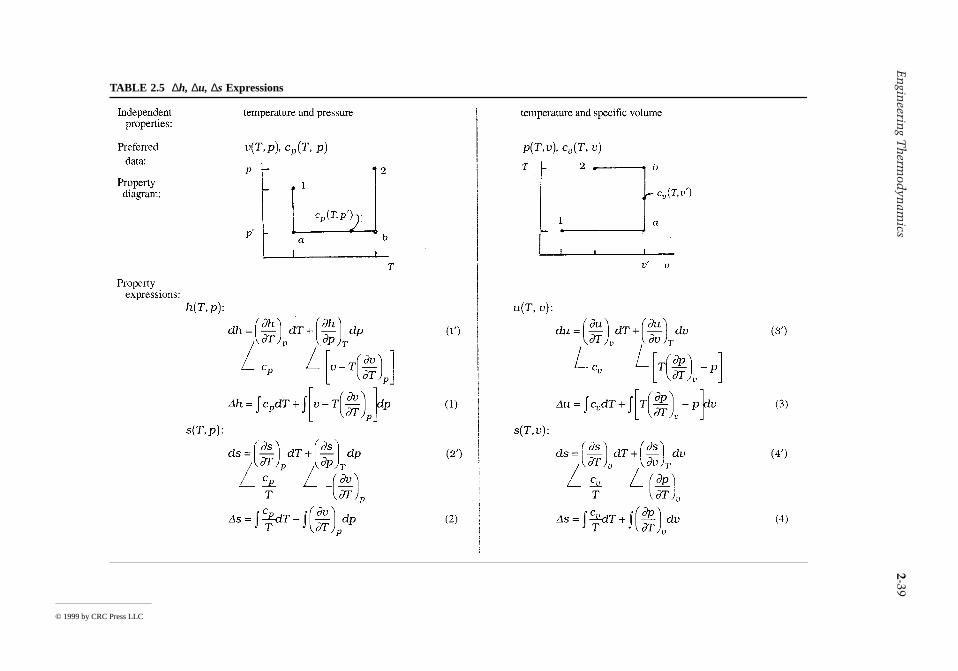
En
gineerin
g Th
ermod
ynam
ics2-39
© 199
9 by CRC Press LLCTABLE 2.5 ∆h, ∆u, ∆s Expressions
2-40 Section 2
f
ic
nction
s of
ns.operty
ion.
such
es
Since T and v are independent, the coefficients of dT and dv must vanish, giving, respectively,
The first of these corresponds to Equation 1 of Table 2.4 and Equation 4 of Table 2.5. The second ofthe above expressions establishes Equation 3 of Table 2.5. With similar considerations, Equation 3 oTable 2.4 and Equations 1 and 2 of Table 2.5 may be obtained.
Fundamental Thermodynamic Functions
A fundamental thermodynamic function is one that provides a complete description of the thermodynamstate. The functions u(s, v) , h(s, p) , ψ(T, v), and g(T, p) listed in Table 2.2 are fundamental thermodynamicfunctions.
In principle, all properties of interest can be determined from a fundamental thermodynamic fuby differentiation and combination. Taking the function ψ(T, v) as a representative case, the propertiesv and T, being the independent variables, are specified to fix the state. The pressure p and specific entropys at this state can be determined by differentiation of ψ(T, v), as shown in Table 2.2. By definition, ψ =u – Ts, so specific internal energy is obtained as
with u, p, and v known, the specific enthalpy can be found from the definition h = u + pv. Similarly,the specific Gibbs function is found from the definition g = h – Ts. The specific heat cv can be determinedby further differentiation cv = (∂u/∂T)v.
The development of a fundamental function requires the selection of a functional form in termthe appropriate pair of independent properties and a set of adjustable coefficients that may number 50or more. The functional form is specified on the basis of both theoretical and practical consideratioThe coefficients of the fundamental function are determined by requiring that a set of selected prvalues and/or observed conditions be statisfied in a least-squares sense. This generally involves propertydata requiring the assumed functional form to be differentiated one or more times, for example p-v-Tand specific heat data. When all coefficients have been evaluated, the function is tested for accuracy byusing it to evaluate properties for which accepted values are known such as velocity of sound and Joule-Thomson data. Once a suitable fundamental function is established, extreme accuracy in and consistencyamong the thermodynamic properties are possible. The properties of water tabulated by Keenan et al.(1969) and by Haar et al. (1984) have been calculated from representations of the Helmholtz funct
Thermodynamic Data Retrieval
Tabular presentations of pressure, specific volume, and temperature are available for practically importantgases and liquids. The tables normally include other properties useful for thermodynamic analyses,as internal energy, enthalpy, and entropy. The various steam tables included in the references of thischapter provide examples. Computer software for retrieving the properties of a wide range of substancis also available, as, for example, the ASME Steam Tables (1993) and Bornakke and Sonntag (1996).
Ts
Tc dT
u
vp T
p
Tdv
vv
T v
∂∂
∂∂
∂∂
−
=
+ −
∂∂
∂∂
∂∂
s
T
c
T
u
vT
p
Tp
v
v
T v
=
=
−
u Ts= +ψ
© 1999 by CRC Press LLC
Engineering Thermodynamics 2-41
).
tate.
uld beed in
Increasingly, textbooks come with computer disks providing thermodynamic property data for water,certain refrigerants, and several gases modeled as ideal gases — see, e.g., Moran and Shapiro (1996
The sample steam table data presented in Table 2.6 are representative of data available for substancescommonly encountered in mechanical engineering practice. Table A.5 and Figures 2.7 to 2.9 providesteam table data for a greater range of states. The form of the tables and figures, and how they are usedare assumed to be familiar. In particular, the use of linear interpolation with such tables is assumedknown.
Specific internal energy, enthalpy, and entropy data are determined relative to arbitrary datums andsuch datums vary from substance to substance. Referring to Table 2.6a, the datum state for the specificinternal energy and specific entropy of water is seen to correspond to saturated liquid water at 0.01°C(32.02°F), the triple point temperature. The value of each of these properties is set to zero at this sIf calculations are performed involving only differences in a particular specific property, the datumcancels. When there are changes in chemical composition during the process, special care shoexercised. The approach followed when composition changes due to chemical reaction is considerSection 2.4.
Liquid water data (see Table 2.6d) suggests that at fixed temperature the variation of specific volume,internal energy, and entropy with pressure is slight. The variation of specific enthalpy with pressure atfixed temperature is somewhat greater because pressure is explicit in the definition of enthalpy. Thisbehavior for v, u, s, and h is exhibited generally by liquid data and provides the basis for the followingset of equations for estimating property data at liquid states from saturated liquid data:
(2.50a)
(2.50b)
(2.50c)
(2.50d)
As before, the subscript f denotes the saturated liquid state at the temperature T, and psat is the corre-sponding saturation pressure. The underlined term of Equation 2.50c is often negligible, giving h(T, p)≈ hf (T), which is used in Example 3 to evaluate h1.
In the absence of saturated liquid data, or as an alternative to such data, the incompressible modelcan be employed:
(2.51)
This model is also applicable to solids. Since internal energy varies only with temperature, the specificheat cv is also a function of only temperature: cv(T) = du/dT. Although specific volume is constant,enthalpy varies with both temperature and pressure, such that
(2.52)
Differentiation of Equation 2.52 with respect to temperature at fixed pressure gives cp =cv. The commonspecific heat is often shown simply as c. Specific heat and density data for several liquids and solids are
v T p v T,( ) ≈ ( )f
u T p u T,( ) ≈ ( )f
h T p h T v p p Tf sat,( ) ≈ ( ) + − ( )[ ]− − − − − − − − −
f
s T p s T,( ) ≈ ( )f
Incompressible model:constantv
u u T
== ( )
h T p u T pv,( ) = ( ) +
© 1999 by CRC Press LLC
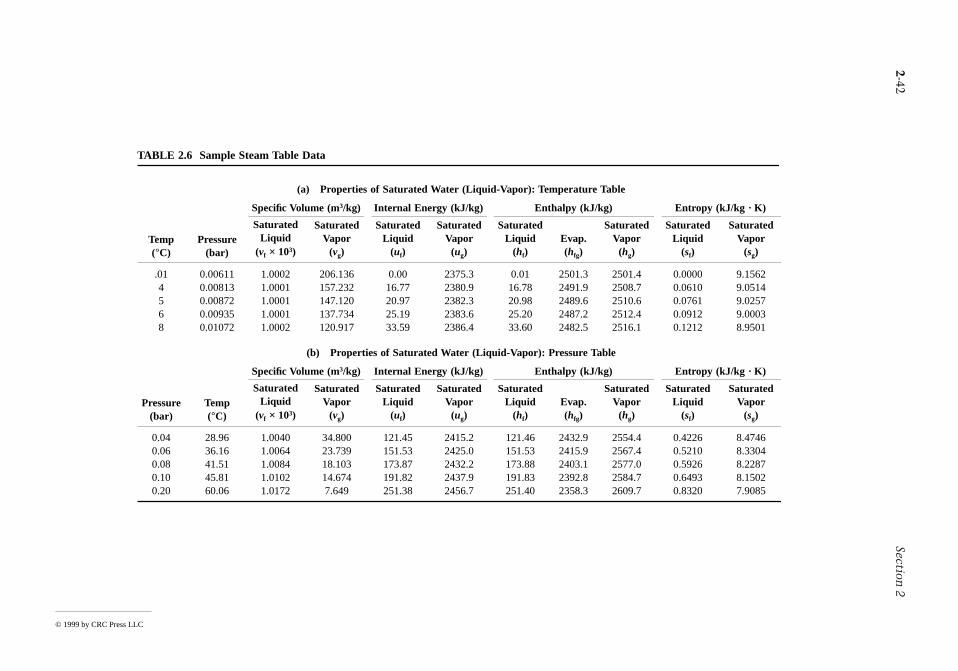
2-42Section
2
© 1999 by CRC Press L
T
Temperature Table
Enthalpy (kJ/kg) Entropy (kJ/kg · K)
dEvap.(hfg)
SaturatedVapor(hg)
SaturatedLiquid
(sf)
Saturated Vapor
(sg)
.01 2501.3 2501.4 0.0000 9.1562.78 2491.9 2508.7 0.0610 9.0514.98 2489.6 2510.6 0.0761 9.0257.20 2487.2 2512.4 0.0912 9.0003.60 2482.5 2516.1 0.1212 8.9501
r): Pressure Table
Enthalpy (kJ/kg) Entropy (kJ/kg · K)
dEvap.(hfg)
SaturatedVapor(hg)
SaturatedLiquid
(sf)
SaturatedVapor
(sg)
1.46 2432.9 2554.4 0.4226 8.47461.53 2415.9 2567.4 0.5210 8.33043.88 2403.1 2577.0 0.5926 8.22871.83 2392.8 2584.7 0.6493 8.15021.40 2358.3 2609.7 0.8320 7.9085
LC
ABLE 2.6 Sample Steam Table Data
(a) Properties of Saturated Water (Liquid-Vapor):
Specific Volume (m3/kg) Internal Energy (kJ/kg)
Temp(°C)
Pressure(bar)
SaturatedLiquid
(vf × 103)
SaturatedVapor
(vg)
SaturatedLiquid
(uf)
SaturatedVapor(ug)
SaturateLiquid
(hf)
.01 0.00611 1.0002 206.136 0.00 2375.3 04 0.00813 1.0001 157.232 16.77 2380.9 165 0.00872 1.0001 147.120 20.97 2382.3 206 0.00935 1.0001 137.734 25.19 2383.6 258 0.01072 1.0002 120.917 33.59 2386.4 33
(b) Properties of Saturated Water (Liquid-Vapo
Specific Volume (m3/kg) Internal Energy (kJ/kg)
Pressure(bar)
Temp(°C)
SaturatedLiquid
(vf × 103)
SaturatedVapor
(vg)
SaturatedLiquid
(uf)
SaturatedVapor(ug)
SaturateLiquid
(hf)
0.04 28.96 1.0040 34.800 121.45 2415.2 120.06 36.16 1.0064 23.739 151.53 2425.0 150.08 41.51 1.0084 18.103 173.87 2432.2 170.10 45.81 1.0102 14.674 191.82 2437.9 190.20 60.06 1.0172 7.649 251.38 2456.7 25
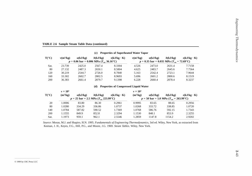
En
gineerin
g Th
ermod
ynam
ics2-43
© 1999 by CRC Press LLC
ter Vapor
/kg) u(kJ/kg) h(kJ/kg) s(kJ/kg · K)p = 0.35 bar = 0.035 MPa (Tsat = 72.69°C)
4.526 2473.0 2631.4 7.71584.625 2483.7 2645.6 7.75645.163 2542.4 2723.1 7.96445.696 2601.2 2800.6 8.15196.228 2660.4 2878.4 8.3237
uid Water
103
kg) u(kJ/kg) h(kJ/kg) s(kJ/kg · K)p = 50 bar = 5.0 MPa (Tsat = 263.99°C)
.9995 83.65 88.65 0.29561.0268 333.72 338.85 1.07201.0768 586.76 592.15 1.7343.1530 848.1 853.9 2.3255
1.2859 1147.8 1154.2 2.9202
rmodynamics, 3rd ed. Wiley, New York, as extracted from , New York.
TABLE 2.6 Sample Steam Table Data (continued)
(c) Properties of Superheated Wa
T(°C) v(m3/kg) u(kJ/kg) h(kJ/kg) s(kJ/kg · K) v(m3
p = 0.06 bar = 0.006 MPa (Tsat 36.16°C)
Sat. 23.739 2425.0 2567.4 8.330480 27.132 2487.3 2650.1 8.5804
120 30.219 2544.7 2726.0 8.7840160 33.302 2602.7 2802.5 8.9693200 36.383 2661.4 2879.7 9.1398
(d) Properties of Compressed Liq
T(°C)v × 103
(m3/kg) u(kJ/kg) h(kJ/kg) s(kJ/kg · K)v × (m3/
p = 25 bar = 2.5 MPa (Tsat 223.99°C)
20 1.0006 83.80 86.30 0.2961 080 1.0280 334.29 336.86 1.0737
140 1.0784 587.82 590.52 1.7369200 1.1555 849.9 852.8 2.3294 1Sat. 1.1973 959.1 962.1 2.5546
Source: Moran, M.J. and Shapiro, H.N. 1995. Fundamentals of Engineering TheKeenan, J. H., Keyes, F.G., Hill, P.G., and Moore, J.G. 1969. Steam Tables. Wiley
2-44 Section 2
h
.
ular
tly
provided in Tables B.2, C.1, and C.2. As the variation of c with temperature is slight, c is frequentlytaken as constant.
When the incompressible model is applied. Equation 2.49 takes the form
(2.53)
Also, as Equation 2.32a reduces to du = Tds, and du = c(T)dT, the change in specific entropy is
(2.54)
Ideal Gas Model
Inspection of the generalized compressibility chart, Figure 2.10, shows that when pR is small, and formany states when TR is large, the value of the compressibility factor Z is close to 1. In other words, forpressures that are low relative to pc, and for many states with temperatures high relative to Tc, thecompressibility factor approaches a value of 1. Within the indicated limits, it may be assumed witreasonable accuracy that Z = 1 — that is,
(2.55a)
where R = /M is the specific gas constant. Other forms of this expression in common use are
(2.55b)
Referring to Equation 3′ of Table 2.5, it can be concluded that (∂u/∂v)T vanishes identically for a gaswhose equation of state is exactly given by Equation 2.55, and thus the specific internal energy dependsonly on temperature. This conclusion is supported by experimental observations beginning with the workof Joule, who showed that the internal energy of air at low density depends primarily on temperature
These considerations allow for an ideal gas model of each real gas: (1) the equation of state is givenby Equation 2.55 and (2) the internal energy and enthalpy are functions of temperature alone. The realgas approaches the model in the limit of low reduced pressure. At other states the actual behavior maydepart substantially from the predictions of the model. Accordingly, caution should be exercised wheninvoking the ideal gas model lest significant error is introduced.
Specific heat data for gases can be obtained by direct measurement. When extrapolated to zeropressure, ideal gas-specific heats result. Ideal gas-specific heats also can be calculated using molecmodels of matter together with data from spectroscopic measurements. Table A.9 provides ideal gas-specific heat data for a number of substances. The following ideal gas-specific heat relations are frequenuseful:
(2.56a)
(2.56b)
h h c T dT v p p
c T T v p p
T
T
ave
2 1 2 1
2 1 2 1
1
2
− = ( ) + −( )
= −( ) + −( )
∫
∆sc T
TdT
cT
T
T
T
ave
= ( )
=
∫1
2
2
1
ln
pv RT pv RT= =or
R
pV nRT pV mRT= =,
c T c T Rp v( ) = ( ) +
ckR
kc
R
kp v=−
=−1 1
,
© 1999 by CRC Press LLC
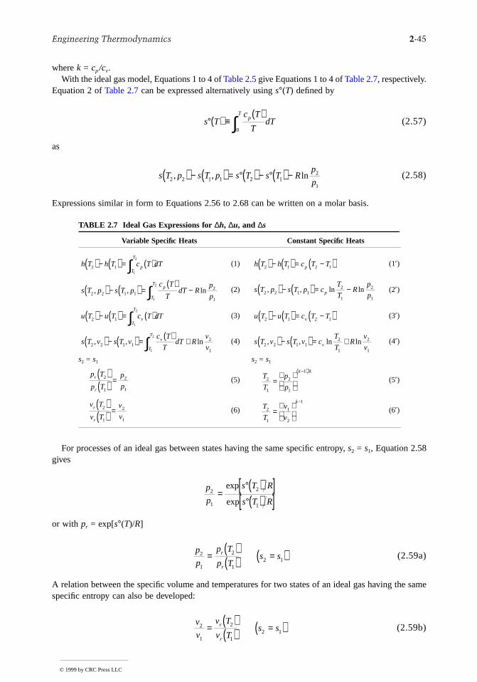
Engineering Thermodynamics 2-45
where k = cp/cv.With the ideal gas model, Equations 1 to 4 of Table 2.5 give Equations 1 to 4 of Table 2.7, respectively.
Equation 2 of Table 2.7 can be expressed alternatively using s°(T) defined by
(2.57)
as
(2.58)
Expressions similar in form to Equations 2.56 to 2.68 can be written on a molar basis.
For processes of an ideal gas between states having the same specific entropy, s2 = s1, Equation 2.58gives
or with pr = exp[s°(T)/R]
(2.59a)
A relation between the specific volume and temperatures for two states of an ideal gas having the samespecific entropy can also be developed:
(2.59b)
TABLE 2.7 Ideal Gas Expressions for ∆h, ∆u, and ∆s
Variable Specific Heats Constant Specific Heats
(1) (1′)
(2) (2′)
(3) (3′)
(4) (4′)
s2 = s1 s2 = s1
(5) (5′)
(6) (6′)
s Tc T
TdTp
T
°( ) ≡( )
∫0
s T p s T p s T s T Rp
p2 2 1 1 2 12
1
, , ln( ) − ( ) = °( ) − °( ) −
h T h T c T dTpT
T
2 11
2( ) − ( ) = ( )∫ h T h T c T Tp2 1 2 1( ) − ( ) = −( )
s T p s T pc T
TdT R
p
pp
T
T
2 2 1 12
11
2
, , ln( ) − ( ) =( )
−∫ s T p s T p cT
TR
p
pp2 2 1 12
1
2
1
, , ln ln( ) − ( ) = −
u T u T c T dTT
T
v2 11
2( ) − ( ) = ( )∫ u T u T c T Tv2 1 2 1( ) − ( ) = −( )
s T v s T vc T
TdT R
v
vv
T
T
2 2 1 12
11
2
, , ln( ) − ( ) =( )
+∫ s T v s T v cT
TR
v
vv2 2 1 12
1
2
1
, , ln ln( ) − ( ) = +
p T
p T
p
pr
r
2
1
2
1
( )( ) = T
T
p
p
k k
2
1
2
1
1
=
−( )
v T
v T
v
vr
r
2
1
2
1
( )( ) = T
T
v
v
k
2
1
1
2
1
=
−
p
p
s T R
s T R2
1
2
1
=°( )[ ]°( )[ ]
exp
exp
p
p
p T
p Ts sr
r
2
1
2
12 1=
( )( ) =( )
v
v
v T
v Ts sr
r
2
1
2
12 1=
( )( ) =( )
© 1999 by CRC Press LLC
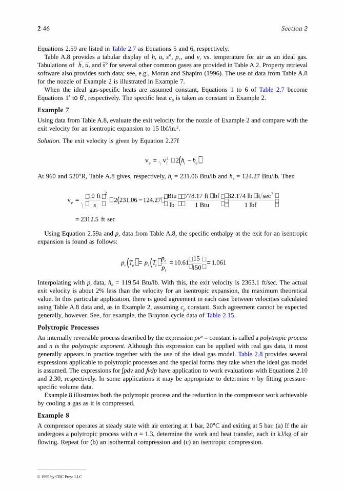
2-46 Section 2
he
l
10
Equations 2.59 are listed in Table 2.7 as Equations 5 and 6, respectively.Table A.8 provides a tabular display of h, u, s°, pr , and vr vs. temperature for air as an ideal gas.
Tabulations of and s° for several other common gases are provided in Table A.2. Property retrievalsoftware also provides such data; see, e.g., Moran and Shapiro (1996). The use of data from Table A.8for the nozzle of Example 2 is illustrated in Example 7.
When the ideal gas-specific heats are assumed constant, Equations 1 to 6 of Table 2.7 becomeEquations 1′ tο 6′, respectively. The specific heat cp is taken as constant in Example 2.
Example 7
Using data from Table A.8, evaluate the exit velocity for the nozzle of Example 2 and compare with texit velocity for an isentropic expansion to 15 lbf/in.2.
Solution. The exit velocity is given by Equation 2.27f
At 960 and 520°R, Table A.8 gives, respectively, hi = 231.06 Btu/lb and he = 124.27 Btu/lb. Then
Using Equation 2.59a and pr data from Table A.8, the specific enthalpy at the exit for an isentropicexpansion is found as follows:
Interpolating with pr data, he = 119.54 Btu/lb. With this, the exit velocity is 2363.1 ft/sec. The actualexit velocity is about 2% less than the velocity for an isentropic expansion, the maximum theoreticavalue. In this particular application, there is good agreement in each case between velocities calculatedusing Table A.8 data and, as in Example 2, assuming cp constant. Such agreement cannot be expectedgenerally, however. See, for example, the Brayton cycle data of Table 2.15.
Polytropic Processes
An internally reversible process described by the expression pvn = constant is called a polytropic processand n is the polytropic exponent. Although this expression can be applied with real gas data, it mostgenerally appears in practice together with the use of the ideal gas model. Table 2.8 provides severalexpressions applicable to polytropic processes and the special forms they take when the ideal gas modelis assumed. The expressions for ∫pdv and ∫vdp have application to work evaluations with Equations 2.and 2.30, respectively. In some applications it may be appropriate to determine n by fitting pressure-specific volume data.
Example 8 illustrates both the polytropic process and the reduction in the compressor work achievableby cooling a gas as it is compressed.
Example 8
A compressor operates at steady state with air entering at 1 bar, 20°C and exiting at 5 bar. (a) If the airundergoes a polytropic process with n = 1.3, determine the work and heat transfer, each in kJ/kg of airflowing. Repeat for (b) an isothermal compression and (c) an isentropic compression.
h u, ,
v ve i i eh h= + −( )2 2
v ft Btu
lb ft lbf
1 Btu2.174 lb ft sec
1 lbf
ft sec
2
e s=
+ −( )
⋅
⋅
=
102 231 06 124 27
778 17 3
2312 5
2
. ..
.
p T p Tp
pr e r ie
i
( ) = ( ) =
=10 61
15150
1 061. .
© 1999 by CRC Press LLC
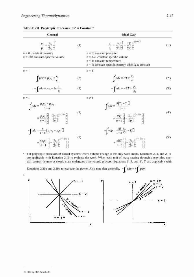
Engineering Thermodynamics 2-47
d 2t, one-
TABLE 2.8 Polytropic Processes: pvn = Constanta
General Ideal Gasb
(1) (1′)
n = 0: constant pressure n = 0: constant pressuren = ±∞: constant specific volume n = ±∞: constant specific volume
n = 1: constant temperaturen = k: constant specific entropy when k is constant
n = 1 n = 1
(2) (2′)
(3) (3′)
n ≠ 1 n ≠ 1
(4) (4′)
(5) (5′)
a For polytropic processes of closed systems where volume change is the only work mode, Equations 2, 4, an′, 4′are applicable with Equation 2.10 to evaluate the work. When each unit of mass passing through a one-inleexit control volume at steady state undergoes a polytropic process, Equations 3, 5, and 3′, 5′ are applicable with
Equations 2.30a and 2.30b to evaluate the power. Also note that generally,
b
p
p
v
v
n
2
1
1
2
=
p
p
v
v
T
T
n n n
2
1
1
2
2
1
1
=
=
−( )
pdv p vv
v1
2
1 12
1∫ = ln pdv RT
v
v1
22
1∫ = ln
− = −∫ vdp p vp
p1
2
1 12
1
ln − = −∫ vdp RTp
p1
22
1
ln
pdvp v p v
n
p v
n
p
p
n n
1
22 2 1 1
1 1 2
1
1
1
11
∫ =−−
=−
−
−( )
pdvR T T
n
RT
n
p
p
n n
1
22 1
1 2
1
1
1
11
∫ =−( )
−
=−
−
−( )
− =−
−( )
=−
−
∫−( )
vdpn
np v p v
np v
n
p
p
n n
1
2
2 2 1 1
1 1 2
1
1
1
11
− =−
−( )
=−
−
∫−( )
vdpnR
nT T
nRT
n
p
p
n n
1
2
2 1
1 2
1
1
1
11
− =∫ ∫1
2
1
2
vdp n pdv.
© 1999 by CRC Press LLC
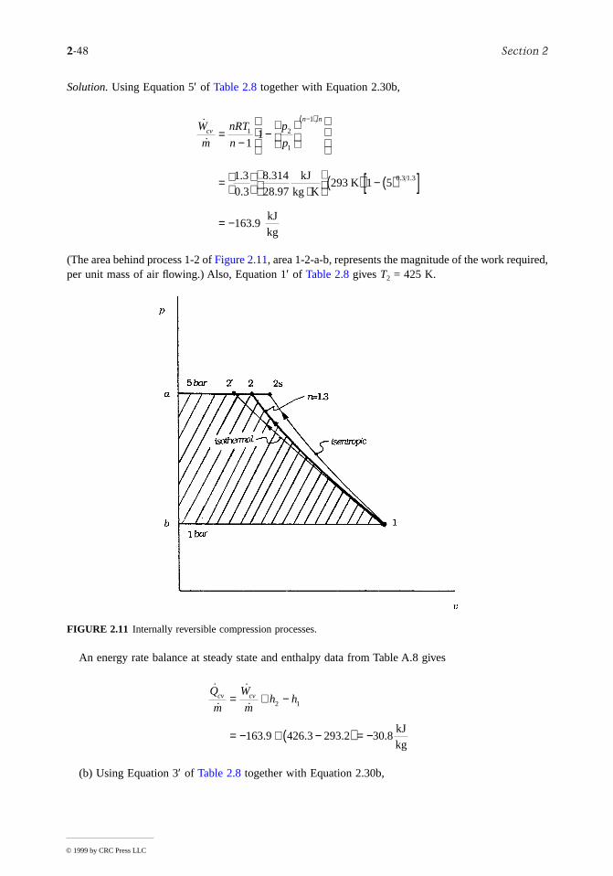
2-48 Section 2
Solution. Using Equation 5′ of Table 2.8 together with Equation 2.30b,
(The area behind process 1-2 of Figure 2.11, area 1-2-a-b, represents the magnitude of the work required,per unit mass of air flowing.) Also, Equation 1′ of Table 2.8 gives T2 = 425 K.
An energy rate balance at steady state and enthalpy data from Table A.8 gives
(b) Using Equation 3′ of Table 2.8 together with Equation 2.30b,
FIGURE 2.11 Internally reversible compression processes.
˙
˙
.
..
.
.
. .
W
m
nRT
n
p
pcv
n n
=−
−
=
⋅
( ) − ( )[ ]
= −
−( )1 2
1
1
0 3 1 3
11
1 30 3
8 31428 97
293 1 5
163 9
kJkg K
K
kJkg
˙
˙
˙
˙
. . . .
Q
m
W
mh hcv cv= + −
= − + −( ) = −
2 1
163 9 426 3 293 2 30 8kJkg
© 1999 by CRC Press LLC
Engineering Thermodynamics 2-49
r
s
ure.t
Area 1-2′-a-b on Figure 2.11 represents the magnitude of the work required, per unit of mass of aiflowing. An energy balance reduces to give = –135.3 kJ/kg. (c) For an isentropiccompression, = 0 and an energy rate balance reduces to give = –(h2s – h1), where 2s denotesthe exit state. With Equation 2.59a and pr data, h2s = 464.8 kJ/kg (T2s = 463K). Then = –(464.8– 293.2) = –171.6 kJ/kg. Area 1-2s-a-b on Figure 2.11 represents the magnitude of the work required,per unit of mass of air flowing.
Ideal Gas Mixtures
When applied to an ideal gas mixture, the additive pressure rule (Section 2.3, p-v-T Relations) is knownas the Dalton model. According to this model, each gas in the mixture acts as if it exists separately atthe volume and temperature of the mixture. Applying the ideal gas equation of state to the mixture aa whole and to each component i, pV = piV = where pi, the partial pressure of componenti, is the pressure that component i would exert if ni moles occupied the full volume V at the temperatureT. Forming a ratio, the partial pressure of component i is
(2.60)
where yi is the mole fraction of component i. The sum of the partial pressures equals the mixture pressThe internal energy, enthalpy, and entropy of the mixture can be determined as the sum of the respecive
properties of the component gases, provided that the contribution from each gas is evaluated at thecondition at which the gas exists in the mixture. On a molar basis,
(2.61a)
(2.61b)
(2.61c)
The specific heats and for an ideal gas mixture in terms of the corresponding specific heats of thecomponents are expressed similarly:
(2.61d)
˙
˙ln
..
ln
.
W
mRT
p
pcv = −
= −
( )
= −
2
1
8 31428 97
293 5
135 3kJkg
˙ / ˙ ˙ / ˙Q m W mcv cv=Qcv
˙ / ˙W mcv˙ / ˙W mcv
nRT, n RTi ,
pn
np y pi
ii= =
U = == =
∑ ∑n u u y ui
i
j
i i
i
j
i
1 1
or
H = == =
∑ ∑n h h y hi
i
j
i i
i
j
i
1 1
or
S = == =
∑ ∑n s s y si
i
j
i i
i
j
i
1 1
or
cv cp
c cv i
i
j
viy==
∑1
© 1999 by CRC Press LLC
2-50 Section 2
andentropynd thease
on,
t fixed
onent.
ssurebulb
ated
(2.61e)
When working on a mass basis, expressions similar in form to Equations 2.61 can be written using massand mass fractions in place of moles and mole fractions, respectively, and using u, h, s, cp, and cv inplace of and respectively.
The internal energy and enthalpy of an ideal gas depend only on temperature, and thus the terms appearing in Equations 2.61 are evaluated at the temperature of the mixture. Since
depends on two independent properties, the terms are evaluated either at the temperature apartial pressure pi of component i, or at the temperature and volume of the mixture. In the former c
(2.62)
Inserting the expressions for H and S given by Equations 2.61b and 2.61c into the Gibbs functiG = H – TS,
(2.63)
where the molar-specific Gibbs function of component i is gi(T, pi) = hi(T) – Tsi(T, pi). The Gibbs functionof i can be expressed alternatively as
(2.64)
were p′ is some specified pressure. Equation 2.64 is obtained by integrating Equation 2.32d atemperature T from pressure p′ to pi.
Moist Air
An ideal gas mixture of particular interest for many practical applications is moist air. Moist air refersto a mixture of dry air and water vapor in which the dry air is treated as if it were a pure compIdeal gas mixture principles usually apply to moist air. In particular, the Dalton model is applicable, andso the mixture pressure p is the sum of the partial pressures pa and pv of the dry air and water vapor,respectively.
Saturated air is a mixture of dry air and saturated water vapor. For saturated air, the partial preof the water vapor equals psat(T), which is the saturation pressure of water corresponding to the dry-(mixture) temperature T. The makeup of moist air can be described in terms of the humidity ratio (specifichumidity) and the relative humidity. The bulb of a wet-bulb thermometer is covered with a wick saturatedwith liquid water, and the wet-bulb temperature of an air-water vapor mixture is the temperature indicby such a thermometer exposed to the mixture.
c cp i
i
j
piy==
∑1
u h s p, , , ,c cV ,ui
hi
si
S = ( )
= ( )
=
=
∑
∑
n s T p
n s T x p
i
i
j
i i
i
i
j
i i
1
1
,
,
G = ( ) − ( )
= ( )
= =
=
∑ ∑
∑
n h T T n s T p
n g T p
i
i
j
i i
i
j
i i
i
i
j
i i
1 1
1
,
,
g T p g T p RT p p
g T p RT x p p
i i i i
i i
, , ln
, ln
( ) = ′( ) + ′( )= ′( ) + ′( )
© 1999 by CRC Press LLC
Engineering Thermodynamics 2-51
sample
les and
ng,
the
nter
pe
When a sample of moist air is cooled at constant pressure, the temperature at which the becomes saturated is called the dew point temperature. Cooling below the dew point temperature resultsin the condensation of some of the water vapor initially present. When cooled to a final equilibriumstate at a temperature below the dew point temperature, the original sample would consist of a gas phaseof dry air and saturated water vapor in equilibrium with a liquid water phase.
Psychrometric charts are plotted with various moist air parameters, including the dry-bulb and wet-bulb temperatures, the humidity ratio, and the relative humidity, usually for a specified value of themixture pressure such as 1 atm. Further discussion of moist air and related psychrometric principapplications is provided in Chapter 9.
Generalized Charts for Enthalpy, Entropy, and Fugacity
The changes in enthalpy and entropy between two states can be determined in principle by correctithe respective property change determined using the ideal gas model. The corrections can be obtainedat least approximately, by inspection of the generalized enthalpy correction and entropy correction charts,Figures 2.12 and 2.13, respectively. Such data are also available in tabular form (see, e.g., Reid andSherwood, 1966) and calculable using a generalized equation for the compressibility factor (Reynolds,1979). Using the superscript * to identify ideal gas property values, the changes in specific enthalpy andspecific entropy between states 1 and 2 are
(2.65a)
(2.65b)
The first underlined term on the right side of each expression represents the respective property changeassuming ideal gas behavior. The second underlined term is the correction that must be applied toideal gas value to obtain the actual value. The quantities and at state 1 wouldbe read from the respective correction chart or table or calculated, using the reduced temperature TR1
and reduced pressure pR1 corresponding to the temperature T1 and pressure p1 at state 1, respectively.Similarly, and at state 2 would be obtained using TR2 and pR2. Mixture valuesfor Tc and pc determined by applying Kay’s rule or some other mixture rule also can be used to ethe generalized enthalpy correction and entropy correction charts.
Figure 2.14 gives the fugacity coefficient, f/p, as a function of reduced pressure and reduced temr-ature. The fugacity f plays a similar role in determining the specific Gibbs function for a real gas aspressure plays for the ideal gas. To develop this, consider the variation of the specific Gibbs functionwith pressure at fixed temperature (from Table 2.2)
For an ideal gas, integration at fixed temperature gives
where C(T) is a function of integration. To evaluate g for a real gas, fugacity replaces pressure,
h h h h RTh h
RT
h h
RTcc c
2 1 2 1
2 1
− = − − −
− −
* ** *
s s s s Rs s
R
s s
R2 1 2 12 1
− = − − −
− −
* ** *
( ) /*h h RTc− ( ) /*s s R−
( ) /*h h RTc− ( ) /*s s R−
∂∂g
pv
T
=
g RT p C T* ln= + ( )
© 1999 by CRC Press LLC
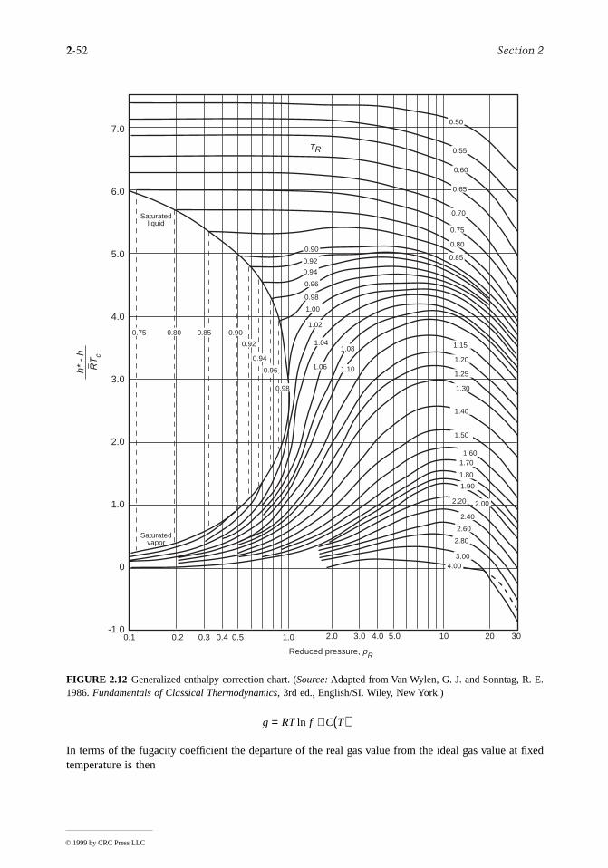
2-52 Section 2
t fixed
.
In terms of the fugacity coefficient the departure of the real gas value from the ideal gas value atemperature is then
FIGURE 2.12 Generalized enthalpy correction chart. (Source: Adapted from Van Wylen, G. J. and Sonntag, R. E1986. Fundamentals of Classical Thermodynamics, 3rd ed., English/SI. Wiley, New York.)
7.0
6.0
5.0
4.0
3.0
2.0
1.0
0
-1.0
Reduced pressure, pR
0.1 0.2 0.3 0.4 0.5 1.0 2.0 3.0 4.0 5.0 10 20 30
h* -
hR
Tc
Saturatedvapor
Saturatedliquid
TR
2.00
1.80
1.60
1.50
1.40
1.30
1.20
1.15
1.10
1.08
1.06
1.04
1.02
1.00
0.98
0.96
0.94
0.92
0.900.85
0.80
0.75
0.70
0.60
0.65
0.55
0.50
1.25
1.70
1.90
2.20
2.40
2.60
2.80
3.004.00
0.75 0.80 0.85 0.90
0.92
0.94
0.96
0.98
g RT f C T= + ( )ln
© 1999 by CRC Press LLC
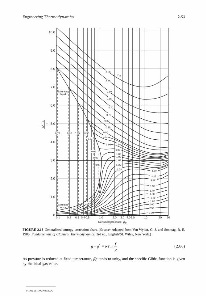
Engineering Thermodynamics 2-53
n
.
(2.66)
As pressure is reduced at fixed temperature, f/p tends to unity, and the specific Gibbs function is giveby the ideal gas value.
FIGURE 2.13 Generalized entropy correction chart. (Source: Adapted from Van Wylen, G. J. and Sonntag, R. E1986. Fundamentals of Classical Thermodynamics, 3rd ed., English/SI. Wiley, New York.)
Reduced pressure, pR
0.1 0.2 0.3 0.4 0.5 1.0 2.0 3.0 4.05.0 10 20 30
10.0
9.0
8.0
7.0
6.0
5.0
4.0
3.0
2.0
1.0
0
Saturatedvapor
Saturatedliquid
S*
- S
R
TR
2.001.801.60
1.501.40
1.30
1.20
1.15
1.101.08
1.06
1.041.021.00
0.98
0.96 0.94
0.92
0.90
0.85
0.80
0.75
0.70
0.60
2.50
3.00
0.65
0.55
0.50
0.75 0.80 0.85 0.90
0.92
0.94
0.96
0.98
0.90
0.95
g g RTf
p− =* ln
© 1999 by CRC Press LLC
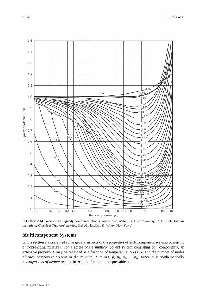
2-54 Section 2
onsisting
moles
Reduced pressure, pR
0.1
1.5
1.4
1.3
1.2
1.1
1.0
0.9
0.8
0.7
0.6
0.5
0.4
0.3
0.2
0.1
00.2 0.3 0.4 0.5 1.0 2.0 3.0 4.0 5.0 10 20 30
Fug
acity
coe
ffici
ent,
f/p
15.00
10.00
6.00
2.001.90
1.80
1.70
1.60
1.50
1.45
1.40
1.35
1.30
1.25
1.20
1.15
1.101.08
1.061.04
1.021.00
0.980.96
0.940.92
0.90
0.850.80
0.750.70 0.60
0.60
0.65
0.70
0.75
0.800.85 0.90
Saturation line
TR
Multicomponent Systems
In this section are presented some general aspects of the properties of multicomponent systems cof nonreacting mixtures. For a single phase multicomponent system consisting of j components, anextensive property X may be regarded as a function of temperature, pressure, and the number ofof each component present in the mixture: X = X(T, p, n1, n2, … nj). Since X is mathematicallyhomogeneous of degree one in the n’s, the function is expressible as
FIGURE 2.14 Generalized fugacity coefficient chart. (Source: Van Wylen, G. J. and Sonntag, R. E. 1986. Funda-mentals of Classical Thermodynamics, 3rd ed., English/SI. Wiley, New York.)
© 1999 by CRC Press LLC
Engineering Thermodynamics 2-55
bbs
changes
py of
(2.67)
where the partial molar property is by definition
(2.68)
and the subscript n, denotes that all n’s except ni are held fixed during differentiation. As dependsin general on temperature, pressure, and mixture composition: (T, p, n1, n2, … nj), the partial molalproperty is an intensive property of the mixture and not simply a property of the ith component.
Selecting the extensive property X to be volume, internal energy, enthalpy, entropy, and the Gifunction, respectively, gives
(2.69)
where and denote the respective partial molal properties.When pure components, each initially at the same temperature and pressure, are mixed, the
in volume, internal energy, enthalpy, and entropy on mixing are given by
(2.70a)
(2.70b)
(2.70c)
(2.70d)
where and denote the molar-specific volume, internal energy, enthalpy, and entropure component i.
Chemical Potential
The partial molal Gibbs function of the ith component of a multicomponent system is the chemicalpotential, µi,
X n Xi i
i
j
==
∑1
Xi
XX
nii T p n
=
∂∂
, , l
Xi
Xi
Xi
V n V U n U
H n H S n S
G n G
i i
i
j
i i
i
j
i i
i
j
i i
i
j
i i
i
j
= =
= =
=
= =
= =
=
∑ ∑
∑ ∑
∑
1 1
1 1
1
,
,
V U H Si i i i, , , , Gi
∆V n V vi i i
i
j
mixing = −( )=
∑1
∆U n U ui i i
i
j
mixing = −( )=
∑1
∆H n H hi i i
i
j
mixing = −( )=
∑1
∆S n S si i i
i
j
mixing = −( )=
∑1
v u hi i i, , , si
© 1999 by CRC Press LLC
2-56 Section 2
sests s
:ce to the
rily
say
wo
y ofbrium,m).
s.
nd
(2.71)
Like temperature and pressure, the chemical potential, µi is an intensive property.When written in terms of chemical potentials, Equation 2.67 for the Gibbs function reads
(2.72)
For a single component sysrem, Equation 2.72 reduces to G = nµ; that is, the chemical potential equalthe molar Gibbs function. For an ideal gas mixture, comparison of Equations 2.63 and 2.72 suggµi
= (T, pi); that is, the chemical potential of component i in an ideal gas mixture equals its Gibbfunction per mole of gas i evaluated at the mixture temperature and the partial pressure of the ith gasof the mixture.
The chemical potential is a measure of the escaping tendency of a substance in a multiphase systema substance tends to move from the phase having the higher chemical potential for that substanphase having a lower chemical potential. A necessary condition for phase equilibrium is that the chemicalpotential of each component has the same value in every phase.
The Gibbs phase rule gives the number F of independent intensive properties that may be arbitraspecified to fix the intensive state of a system at equilibrium consisting of N nonreacting componentspresent in P phases: F = 2 + N – P. F is called the degrees of freedom (or the variance). For water asa single component, for example, N = 1 and F = 3 – P.
• For a single phase, P = 1 and F = 2: two intensive properties can be varied independently, temperature and pressure, while maintaining a single phase.
• For two phases, P = 2 and F = 1: only one intensive property can be varied independently if tphases are maintained — for example, temperature or pressure.
• For three phases, P = 3 and F = 0: there are no degrees of freedom; each intensive properteach phase is fixed. For a system consisting of ice, liquid water, and water vapor at equilithere is a unique temperature: 0.01°C (32.02°F) and a unique pressure: 0.6113 kPa (0.006 at
The phase rule does not address the relative amounts that may be present in the various phaseWith G = H – TS and H = U + pV, Equation 2.72 can be expressed as
(2.73)
from which can be derived
(2.74)
When the mixture composition is constant, Equation 2.74 reduces to Equation 2.31a.
Ideal Solution
The Lewis-Randall rule states that the fugacity of each component i in an ideal solution is the productof its mole fraction and the fugacity of the pure component, fi, at the same temperature, pressure, astate of aggregation (gas, liquid, or solid) as the mixture:
µ ∂∂i i
i T p n
GG
n= =
, , l
G ni i
i
j
==
∑ µ1
gi
U TS pV ni i
i
j
= − +=
∑ µ1
dU TdS pdV dni i
i
j
= − +=
∑µ1
fi
© 1999 by CRC Press LLC
Engineering Thermodynamics 2-57
se, mixing
ofl
nt ures are, IdealLewis-
(2.75)
The following characteristics are exhibited by an ideal solution: With theEquations 2.70a, b, and c show that there is no change in volume, internal energy, or enthalpy onpure components to form an ideal solution. The adiabatic mixing of different pure components wouldresult in an increase in entropy, however, because such a process is irreversible.
The volume of an ideal solution is
(2.76)
where Vi is the volume that pure component i would occupy when at the temperature and pressurethe mixture. Comparing Equations 2.48a and 2.76, the additive volume rule is seen to be exact for ideasolutions. The internal energy and enthalpy of an ideal solution are
(2.77)
where and denote, respectively, the molar internal energy and enthalpy of pure componei atthe temperature and pressure of the mixture. Many gaseous mixtures at low to moderate pressadequately modeled by the Lewis Randall rule. The ideal gas mixtures considered in Section 2.3Gas Model, is an important special case. Some liquid solutions also can be modeled with the Randall rule.
f y fi i i= ( )Lewis-Randall rule
V v U u H hi i i i i i= = =, , .
V n v Vi i
i
j
i
i
j
= = ( )= =
∑ ∑1 1
ideal solution
U n u H n hi i
i
j
i i
i
j
= = ( )= =
∑ ∑,1 1
ideal solution
ui hi
© 1999 by CRC Press LLC
2-58 Section 2
ted innthalpy
eleaseommonbutor
r, andas coal. pro-itions ofions,
hemicalstituentions.ds. Thestion
itrogen,
one. In
only byition of
roducts for allanalysis
in theooled atenr when
ations Ideali-r thangenstiontion or
res are.
2.4 Combustion
The thermodynamic analysis of reactive systems is primarily an extension of principles presenSections 2.1 to 2.3. It is necessary, though, to modify the methods used to evaluate specific eand entropy.
Reaction Equations
In combustion reactions, rapid oxidation of combustible elements of the fuel results in energy ras combustion products are formed. The three major combustible chemical elements in most cfuels are carbon, hydrogen, and sulfur. Although sulfur is usually a relatively unimportant contrito the energy released, it can be a significant cause of pollution and corrosion.
The emphasis in this section is on hydrocarbon fuels, which contain hydrogen, carbon, sulfupossibly other chemical substances. Hydrocarbon fuels may be liquids, gases, or solids such Liquid hydrocarbon fuels are commonly derived from crude oil through distillation and crackingcesses. Examples are gasoline, diesel fuel, kerosene, and other types of fuel oils. The composliquid fuels are commonly given in terms of mass fractions. For simplicity in combustion calculatgasoline is often considered to be octane, C8H18, and diesel fuel is considered to be dodecane, C12H26.Gaseous hydrocarbon fuels are obtained from natural gas wells or are produced in certain cprocesses. Natural gas normally consists of several different hydrocarbons, with the major conbeing methane, CH4. The compositions of gaseous fuels are commonly given in terms of mole fractBoth gaseous and liquid hydrocarbon fuels can be synthesized from coal, oil shale, and tar sancomposition of coal varies considerably with the location from which it is mined. For combucalculations, the makeup of coal is usually expressed as an ultimate analysis giving the composition ona mass basis in terms of the relative amounts of chemical elements (carbon, sulfur, hydrogen, noxygen) and ash. Coal combustion is considered further in Chapter 8, Energy Conversion.
A fuel is said to have burned completely if all of the carbon present in the fuel is burned to carbdioxide, all of the hydrogen is burned to water, and all of the sulfur is burned to sulfur dioxidpractice, these conditions are usually not fulfilled and combustion is incomplete. The presence of carbonmonoxide (CO) in the products indicates incomplete combustion. The products of combustion of actualcombustion reactions and the relative amounts of the products can be determined with certainty experimental means. Among several devices for the experimental determination of the composproducts of combustion are the Orsat analyzer, gas chromatograph, infrared analyzer, and flame ion-ization detector. Data from these devices can be used to determine the makeup of the gaseous pof combustion. Analyses are frequently reported on a “dry” basis: mole fractions are determinedgaseous products as if no water vapor were present. Some experimental procedures give an including the water vapor, however.
Since water is formed when hydrocarbon fuels are burned, the mole fraction of water vapor gaseous products of combustion can be significant. If the gaseous products of combustion are cconstant mixture pressure, the dew point temperature (Section 2.3, Ideal Gas Model) is reached whwater vapor begins to condense. Corrosion of duct work, mufflers, and other metal parts can occuwater vapor in the combustion products condenses.
Oxygen is required in every combustion reaction. Pure oxygen is used only in special applicsuch as cutting and welding. In most combustion applications, air provides the needed oxygen.zations are often used in combustion calculations involving air: (1) all components of air otheoxygen (O2) are lumped with nitrogen (N2). On a molar basis air is then considered to be 21% oxyand 79% nitrogen. With this idealization the molar ratio of the nitrogen to the oxygen in combuair is 3.76; (2) the water vapor present in air may be considered in writing the combustion equaignored. In the latter case the combustion air is regarded as dry; (3) additional simplicity results byregarding the nitrogen present in the combustion air as inert. However, if high-enough temperatuattained, nitrogen can form compounds, often termed NOX, such as nitric oxide and nitrogen dioxide
© 1999 by CRC Press LLC
Engineering Thermodynamics 2-59
es can
ll theton the
Anothertions
assture of
mical
d 100 is
productlosure
Even trace amounts of oxides of nitrogen appearing in the exhaust of internal combustion enginbe a source of air pollution.
The minimum amount of air that supplies sufficient oxygen for the complete combustion of acombustible chemical elements is the theoretical, or stoichiometic, amount of air. In practice, the amounof air actually supplied may be greater than or less than the theoretical amount, depending application. The amount of air is commonly expressed as the percent of theoretical air or the percentexcess (or percent deficiency) of air. The air-fuel ratio and its reciprocal the fuel-air ratio, each of whichcan be expressed on a mass or molar basis, are other ways that fuel-air mixtures are described.is the equivalence ratio: the ratio of the actual fuel-air ratio to the fuel-air ratio for complete combuswith the theoretical amount of air. The reactants form a lean mixture when the equivalence ratio is lesthan unity and a rich mixture when the ratio is greater than unity.
Example 9
Methane, CH4, is burned with dry air. The molar analysis of the products on a dry basis is CO2, 9.7%;CO, 0.5%; O2, 2.95%; and N2, 86.85%. Determine (a) the air-fuel ratio on both a molar and a mbasis, (b) the percent of theoretical air, (c) the equivalence ratio, and (d) the dew point temperathe products, in °F, if the pressure is 1 atm.
Solution.(a) The solution is conveniently conducted on the basis of 100 lbmol of dry products. The che
equation then reads
where N2 is regarded as inert. Water is included in the products together with the assumelbmol of dry products. Balancing the carbon, hydrogen, and oxygen, the reaction equation
The nitrogen also balances, as can be verified. This checks the accuracy of both the given analysis and the calculations conducted to determine the unknown coefficients. Exact ccannot be expected with measured data, however. On a molar basis, the air-fuel ratio is
On a mass basis
(b) The balanced chemical equation for the complete combustion of methane with the theoreticalamount of air is
The theoretical air-fuel ratio on a molar basis is
a b cCH O N CO CO O N H O4 2 2 2 2 2 2+ +( ) → + + + +3 76 9 7 0 5 2 95 86 85. . . . .
10 2 23 1 3 76 9 7 0 5 2 95 86 85 20 4. . . . . . . .CH O N CO CO O N H O4 2 2 2 2 2 2+ +( ) → + + + +
AFlbmol air
lbmol fuel= ( ) = ( )
( )23 1 4 76
10 210 78
. .
..
AFlb air
lb fuel= ( )
= ( )
( )10 78
28 9716 04
19 47...
.
CH O N CO H O + 7.52N4 2 2 2 2 2+ +( ) → +2 3 76 2.
AFlbmol air
lbmol fuel( ) = ( ) = ( )
( )theo
2 4 76
19 52
..
© 1999 by CRC Press LLC
2-60 Section 2
tss
es
e.
ed
er in
molarl
The percent theoretical air is then
(c) Equivalence ratio = = 9.52/10.78 = 0.88. The reactants form a lean mixture.(d) To determine the dew point temperature requires the partial pressure pv of the water vapor. The
mole fraction of the water vapor is
Since p = 1 atm, pv = 0.169 atm = 2.48 lbf/in.2. With psat = 2.48 lbf/in.2, the correspondingsaturation temperature from the steam tables is 134°F. This is the dew point temperature.
Property Data for Reactive Systems
Tables of thermodynamic properties such as the steam tables provide values for the specific enthalpyand entropy relative to some arbitrary datum state where the enthalpy (or alternatively the internal energy)and entropy are set to zero. When a chemical reaction occurs, however, reactants disappear and producare formed, and it is generally no longer possible to evaluate and so that these arbitrary datumcancel. Accordingly, special means are required to assign specific enthalpy and entropy for applicationto reacting systems.
Property data suited for the analysis of reactive systems are available from several sources. Theencyclopedic JANAF Thermochemical Tables is commonly used. Data for a wide range of substancare retrievable from Knacke et al. (1991), which provides both tabular data and analytical expressionsreadily programmable for use with personal computers of the specific heat, enthalpy, entropy, and Gibbsfunction. Textbooks on engineering thermodynamics also provide selected data, as, for example, Moranand Shapiro (1995).
Enthalpy of Formation
An enthalpy datum for reacting systems can be established by assigning arbitrarily a value of zero tothe enthalpy of the stable elements at a standard reference state where the temperature is Tref = 298.15K (25°C) and the pressure is pref , which may be 1 bar or 1 atm depending on the data source. The termstable simply means that the particular element is chemically stable. For example, at the standard statthe stable forms of hydrogen, oxygen, and nitrogen are H2, O2, and N2 and not the monatomic H, O, and N
The molar enthalpy of a compound at the standard state equals its enthalpy of formation, symbolizedhere by The enthalpy of formation is the energy released or absorbed when the compound is formfrom its elements, the compound and elements all being at Tref and pref . The enthalpy of formation maybe determined by application of procedures from statistical thermodynamics using observed spectro-scopic data. The enthalpy of formation also can be found in principle by measuring the heat transfa reaction in which the compound is formed from the elements. In this chapter, the superscript ° is usedto denote pref . For the case of the enthalpy of formation, the reference temperature Tref is also intendedby this symbol. Table 2.9 gives the values of the enthalpy of formation of various substances at 298 Kand 1 atm.
The molar enthalpy of a substance at a state other than the standard state is found by adding theenthalpy change between the standard state and the state of interest to the molar enthapy offormation:
%
..
. %
theoretical air =AF
AF
( )( )
= = ( )
theo
10 789 52
1 13 113
( )/( )FA FA theo
yv =+
=20 4100 20 4
0 169.
..
∆h ∆s
hf
o.
∆h
© 1999 by CRC Press LLC
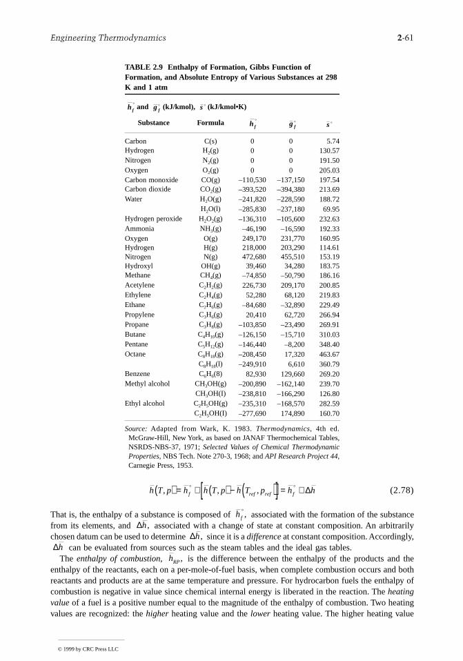
Engineering Thermodynamics 2-61
bstancearily,
thend boththalpy of
eatinge
(2.78)
That is, the enthalpy of a substance is composed of associated with the formation of the sufrom its elements, and associated with a change of state at constant composition. An arbitrchosen datum can be used to determine since it is a difference at constant composition. Accordingly
can be evaluated from sources such as the steam tables and the ideal gas tables.The enthalpy of combustion, is the difference between the enthalpy of the products and
enthalpy of the reactants, each on a per-mole-of-fuel basis, when complete combustion occurs areactants and products are at the same temperature and pressure. For hydrocarbon fuels the encombustion is negative in value since chemical internal energy is liberated in the reaction. The heatingvalue of a fuel is a positive number equal to the magnitude of the enthalpy of combustion. Two hvalues are recognized: the higher heating value and the lower heating value. The higher heating valu
TABLE 2.9 Enthalpy of Formation, Gibbs Function of Formation, and Absolute Entropy of Various Substances at 298 K and 1 atm
and (kJ/kmol), (kJ/kmol•K)
Substance Formula
Carbon C(s) 0 0 5.74Hydrogen H2(g) 0 0 130.57Nitrogen N2(g) 0 0 191.50Oxygen O2(g) 0 0 205.03Carbon monoxide CO(g) –110,530 –137,150 197.54Carbon dioxide CO2(g) –393,520 –394,380 213.69Water H2O(g) –241,820 –228,590 188.72
H2O(l) –285,830 –237,180 69.95Hydrogen peroxide H2O2(g) –136,310 –105,600 232.63Ammonia NH3(g) –46,190 –16,590 192.33Oxygen O(g) 249,170 231,770 160.95Hydrogen H(g) 218,000 203,290 114.61Nitrogen N(g) 472,680 455,510 153.19Hydroxyl OH(g) 39,460 34,280 183.75Methane CH4(g) –74,850 –50,790 186.16Acetylene C2H2(g) 226,730 209,170 200.85Ethylene C2H4(g) 52,280 68,120 219.83Ethane C2H6(g) –84,680 –32,890 229.49Propylene C3H6(g) 20,410 62,720 266.94Propane C3H8(g) –103,850 –23,490 269.91Butane C4H10(g) –126,150 –15,710 310.03Pentane C5H12(g) –146,440 –8,200 348.40Octane C8H18(g) –208,450 17,320 463.67
C8H18(l) –249,910 6,610 360.79Benzene C6H6(8) 82,930 129,660 269.20Methyl alcohol CH3OH(g) –200,890 –162,140 239.70
CH3OH(I) –238,810 –166,290 126.80Ethyl alcohol C2H5OH(g) –235,310 –168,570 282.59
C2H5OH(I) –277,690 174,890 160.70
Source:Adapted from Wark, K. 1983. Thermodynamics, 4th ed.McGraw-Hill, New York, as based on JANAF Thermochemical Tables,NSRDS-NBS-37, 1971; Selected Values of Chemical ThermodynamicProperties, NBS Tech. Note 270-3, 1968; and API Research Project 44,Carnegie Press, 1953.
hf
o
g f
o s
o
hf
o
g f
o
so
h T p h h T p h T p h hf ref ref f, , ,( ) = + ( ) − ( )[ ] = +o o ∆
hf
o,
∆h ,∆h ,
∆hhRP ,
© 1999 by CRC Press LLC
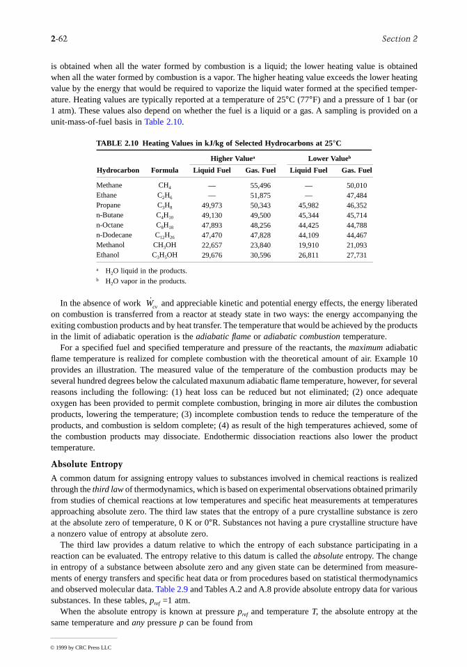
2-62 Section 2
r
e
he
eso
a
re-namics
is obtained when all the water formed by combustion is a liquid; the lower heating value is obtainedwhen all the water formed by combustion is a vapor. The higher heating value exceeds the lower heatingvalue by the energy that would be required to vaporize the liquid water formed at the specified temper-ature. Heating values are typically reported at a temperature of 25°C (77°F) and a pressure of 1 bar (o1 atm). These values also depend on whether the fuel is a liquid or a gas. A sampling is provided on aunit-mass-of-fuel basis in Table 2.10.
In the absence of work and appreciable kinetic and potential energy effects, the energy liberatedon combustion is transferred from a reactor at steady state in two ways: the energy accompanying theexiting combustion products and by heat transfer. The temperature that would be achieved by the productsin the limit of adiabatic operation is the adiabatic flame or adiabatic combustion temperature.
For a specified fuel and specified temperature and pressure of the reactants, the maximum adiabaticflame temperature is realized for complete combustion with the theoretical amount of air. Example 10provides an illustration. The measured value of the temperature of the combustion products may beseveral hundred degrees below the calculated maxunum adiabatic flame temperature, however, for severalreasons including the following: (1) heat loss can be reduced but not eliminated; (2) once adequatoxygen has been provided to permit complete combustion, bringing in more air dilutes the combustionproducts, lowering the temperature; (3) incomplete combustion tends to reduce the temperature of tproducts, and combustion is seldom complete; (4) as result of the high temperatures achieved, some ofthe combustion products may dissociate. Endothermic dissociation reactions also lower the producttemperature.
Absolute Entropy
A common datum for assigning entropy values to substances involved in chemical reactions is realizedthrough the third law of thermodynamics, which is based on experimental observations obtained primarilyfrom studies of chemical reactions at low temperatures and specific heat measurements at temperaturapproaching absolute zero. The third law states that the entropy of a pure crystalline substance is zerat the absolute zero of temperature, 0 K or 0°R. Substances not having a pure crystalline structure havea nonzero value of entropy at absolute zero.
The third law provides a datum relative to which the entropy of each substance participating in reaction can be evaluated. The entropy relative to this datum is called the absolute entropy. The changein entropy of a substance between absolute zero and any given state can be determined from measuments of energy transfers and specific heat data or from procedures based on statistical thermodyand observed molecular data. Table 2.9 and Tables A.2 and A.8 provide absolute entropy data for varioussubstances. In these tables, pref =1 atm.
When the absolute entropy is known at pressure pref and temperature T, the absolute entropy at thesame temperature and any pressure p can be found from
TABLE 2.10 Heating Values in kJ/kg of Selected Hydrocarbons at 25°C
Higher Valuea Lower Valueb
Hydrocarbon Formula Liquid Fuel Gas. Fuel Liquid Fuel Gas. Fuel
Methane CH4 — 55,496 — 50,010Ethane C2H6 — 51,875 — 47,484Propane C3H8 49,973 50,343 45,982 46,352n-Butane C4H10 49,130 49,500 45,344 45,714n-Octane C8H18 47,893 48,256 44,425 44,788n-Dodecane C12H26 47,470 47,828 44,109 44,467Methanol CH3OH 22,657 23,840 19,910 21,093Ethanol C3H5OH 29,676 30,596 26,811 27,731
a H2O liquid in the products.b H2O vapor in the products.
Wcv
© 1999 by CRC Press LLC
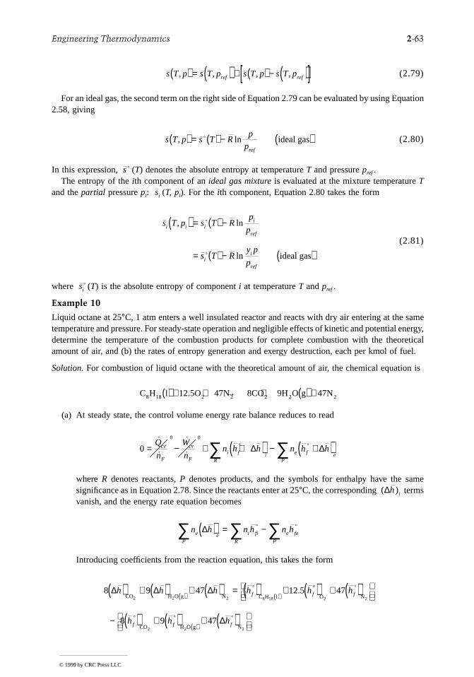
Engineering Thermodynamics 2-63
quation
samel energy,retical
fuel.
n is
ame
(2.79)
For an ideal gas, the second term on the right side of Equation 2.79 can be evaluated by using E2.58, giving
(2.80)
In this expression, (T) denotes the absolute entropy at temperature T and pressure pref .The entropy of the ith component of an ideal gas mixture is evaluated at the mixture temperature T
and the partial pressure pi: (T, pi). For the ith component, Equation 2.80 takes the form
(2.81)
where (T) is the absolute entropy of component i at temperature T and pref .
Example 10
Liquid octane at 25°C, 1 atm enters a well insulated reactor and reacts with dry air entering at thetemperature and pressure. For steady-state operation and negligible effects of kinetic and potentiadetermine the temperature of the combustion products for complete combustion with the theoamount of air, and (b) the rates of entropy generation and exergy destruction, each per kmol of
Solution. For combustion of liquid octane with the theoretical amount of air, the chemical equatio
(a) At steady state, the control volume energy rate balance reduces to read
where R denotes reactants, P denotes products, and the symbols for enthalpy have the ssignificance as in Equation 2.78. Since the reactants enter at 25°C, the corresponding termsvanish, and the energy rate equation becomes
Introducing coefficients from the reaction equation, this takes the form
s T p s T p s T p s T pref ref, , , ,( ) = ( ) + ( ) − ( )[ ]
s T p s T Rp
pref
, ln( ) = ( ) − ( )o ideal gas
so
si
s T p s T Rp
p
s T Ry p
p
i i ii
ref
ii
ref
, ln
ln
( ) = ( ) −
= ( ) − ( )
o
o ideal gas
sio
C H l 12.5O 47N 8CO 9H O g 47N8 18 2 2 2 2 2( ) + + → + ( ) +
00 0
= − + +( ) − +( )∑ ∑˙
˙
˙
˙Q
n
W
nn h h n h hcv
F
cv
Fi f i
R
e f eP
o o∆ ∆
( )∆h i
n h n h n he eP
i fi
R
e fe
P
∆( ) = −∑ ∑ ∑o o
8 9 47 12 5 47
8 9 47
∆ ∆ ∆
∆
h h h h h h
h h h
f f f
f f f
( ) + ( ) + ( ) = ( ) + ( ) + ( )
− ( ) + ( ) + ( )
( ) ( )
( )
CO H O g N C H l O N
CO H O g N
2 2 2 8 18 2 2
2 2 2
o o o
o o o
.
© 1999 by CRC Press LLC
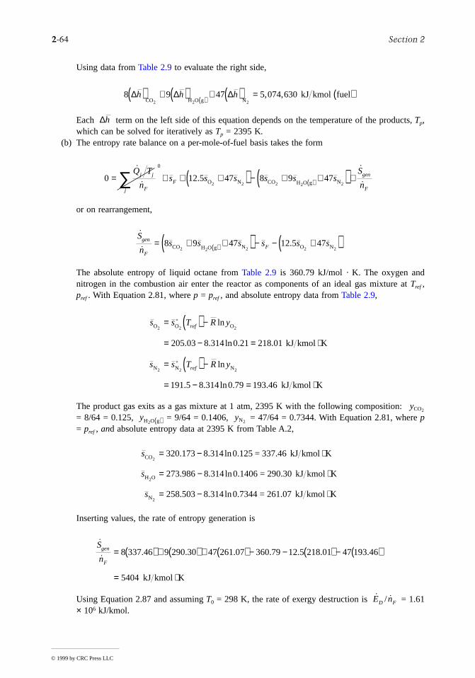
2-64 Section 2
ts
Using data from Table 2.9 to evaluate the right side,
Each term on the left side of this equation depends on the temperature of the produc, Tp,which can be solved for iteratively as Tp = 2395 K.
(b) The entropy rate balance on a per-mole-of-fuel basis takes the form
or on rearrangement,
The absolute entropy of liquid octane from Table 2.9 is 360.79 kJ/mol · K. The oxygen andnitrogen in the combustion air enter the reactor as components of an ideal gas mixture at Tref ,pref . With Equation 2.81, where p = pref , and absolute entropy data from Table 2.9,
The product gas exits as a gas mixture at 1 atm, 2395 K with the following composition: = 8/64 = 0.125, = 9/64 = 0.1406, = 47/64 = 0.7344. With Equation 2.81, where p= pref , and absolute entropy data at 2395 K from Table A.2,
Inserting values, the rate of entropy generation is
Using Equation 2.87 and assuming T0 = 298 K, the rate of exergy destruction is = 1.61× 10⁶ kJ/kmol.
8 9 47∆ ∆ ∆h h h( ) + ( ) + ( ) = ( )( )CO H O g N2 2 2
5,074,630 kJ kmol fuel
∆h
0 12 5 47 8 9 47
0
= + + +( ) − + +( ) +∑ ( )
˙
˙.
˙
˙
Q T
ns s s s s s
S
nj j
Fj
Fgen
FO N CO H O g N2 2 2 2 2
˙
˙.
S
ns s s s s sgen
FF= + +( ) − − +( )( )8 9 47 12 5 47CO H O g N O N2 2 2 2 2
s s T R y
s s T R y
ref
ref
O O O
N N N
2 2 2
2 2 2
kJ kmol K
kJ kmol K
= ( ) −
= − = ⋅
= ( ) −
= − = ⋅
o
o
ln
. . ln . .
ln
. . ln . .
205 03 8 314 0 21 218 01
191 5 8 314 0 79 193 46
yCO2
yH O g2 ( ) yN2
s
s
s
CO
H O
N
2
2
2
320.173 8.314 0.125 = 337.46 kJ kmol K
2 8.314 0.1406 = 290.30 kJ kmol K
2 8.503 8.314 0.7344 = 261.07 kJ kmol K
= − ⋅
= − ⋅
= − ⋅
ln
. ln
ln
73 986
5
˙
˙. . . . . . .
S
ngen
F
= ( ) + ( ) + ( ) − − ( ) − ( )
= ⋅
8 337 46 9 290 30 47 261 07 360 79 12 5 218 01 47 193 46
5404 kJ kmol K
˙ / ˙E nD F
© 1999 by CRC Press LLC
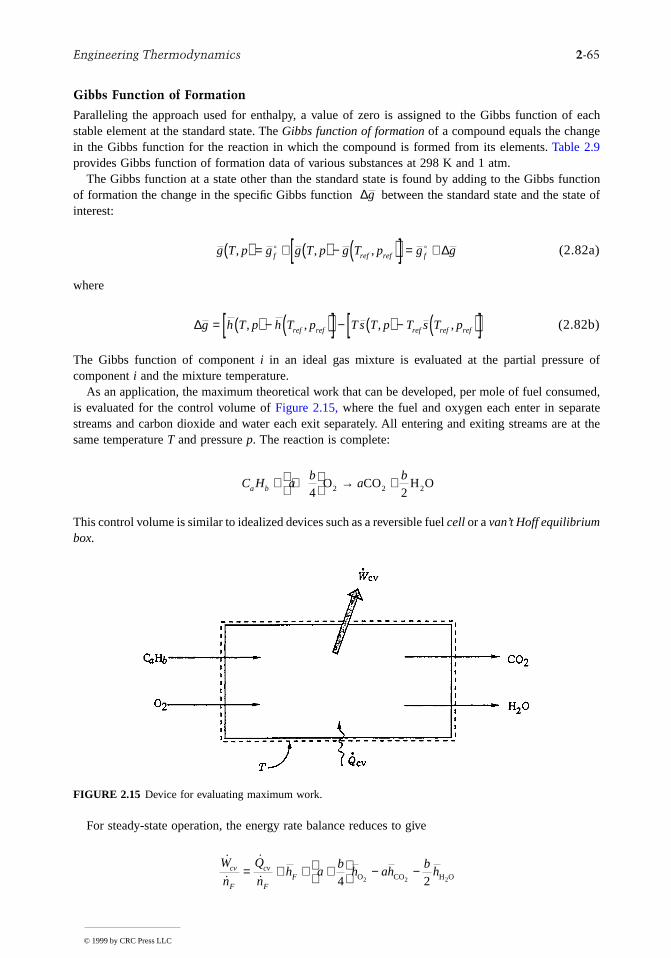
Engineering Thermodynamics 2-65
che
unction of
f
,ate
Gibbs Function of Formation
Paralleling the approach used for enthalpy, a value of zero is assigned to the Gibbs function of eastable element at the standard state. The Gibbs function of formation of a compound equals the changin the Gibbs function for the reaction in which the compound is formed from its elements. Table 2.9provides Gibbs function of formation data of various substances at 298 K and 1 atm.
The Gibbs function at a state other than the standard state is found by adding to the Gibbs fof formation the change in the specific Gibbs function between the standard state and the stateinterest:
(2.82a)
where
(2.82b)
The Gibbs function of component i in an ideal gas mixture is evaluated at the partial pressure ocomponent i and the mixture temperature.
As an application, the maximum theoretical work that can be developed, per mole of fuel consumedis evaluated for the control volume of Figure 2.15, where the fuel and oxygen each enter in separstreams and carbon dioxide and water each exit separately. All entering and exiting streams are at thesame temperature T and pressure p. The reaction is complete:
This control volume is similar to idealized devices such as a reversible fuel cell or a van’t Hoff equilibriumbox.
For steady-state operation, the energy rate balance reduces to give
FIGURE 2.15 Device for evaluating maximum work.
∆g
g T p g g T p g T p g gf ref ref f, , ,( ) = + ( ) − ( )[ ] = +o o ∆
∆g h T p h T p T s T p T s T pref ref ref ref ref= ( ) − ( )[ ] − ( ) − ( )[ ], , , ,
C H ab
ab
a b + +
→ +
4 22O CO H O2 2
˙
˙
˙
˙W
n
Q
nh a
bh ah
bhcv
F
cv
FF= + + +
− −
4 22O CO H O2 2
© 1999 by CRC Press LLC
2-66 Section 2
l:
and
ng
where denotes the molar flow rate of the fuel. Kinetic and potential energy effects are regarded asnegligible. If heat transfer occurs only at the temperature T, an entropy balance for the control volumetakes the form
Eliminating the heat transfer term from these expressions, an expression for the maximum theoreticavalue of the work developed per mole of fuel is obtained when the entropy generation term is set to zero
This can be written alternatively in terms of the enthalpy of combustion as
(2.83a)
or in terms of Gibbs functions as
(2.83b)
Equation 2.83b is used in the solution to Example 11.
Example 11
Hydrogen (H2) and oxygen (O2), each at 25°C, 1 atm, enter a fuel cell operating at steady state, liquid water exits at the same temperature and pressure. The hydrogen flow rate is 2 × 10⁻⁴ kmol/secand the fuel cell operates isothermally at 25°C. Determine the maximum theoretical power the cell candevelop, in kW.
Solution. The overall cell reaction is H2 + 1/2 O2 → H2O(,), and Equations 2.83 are applicable. SelectiEquation 2.83b, and using Gibbs function data from Table 2.9,
Then
nF
04 22
= + + +
− − +
˙ ˙ ˙
˙Q n
Ts a
bs as
bs
S
ncv F
Fgen
FO CO H O2 2
˙
˙, ,
W
nh a
bh ah
bh T p T s a
bs as
bs T pcv
Frev
F F
= + +
− −
( ) − + +
− −
( )
int 4 2 4 22 2O CO H O O CO H O2 2 2 2
˙
˙, ,
W
nh T p T s a
bs as
bs T pcv
Frev
RP F
= − ( ) − + +
− −
( )
int 4 22O CO H O2 2
˙
˙,
W
ng a
bg ag
bg T pcv
Frev
F
= + +
− −
( )
int 4 22O CO H O2 2
˙
˙
, ,
W
ng g gcv
Frev
= + −
°( )
= + ( ) − −( ) =
( )int
H O H O2 2 225 C, 1 atm
kJ kmol
12
012
0 237 180 237 180
l
˙ , .Wcvrev
( ) =
×
=−int 237 180 2 10 47 44kJ
kmolkmol
skW
1kJ s kW
© 1999 by CRC Press LLC
Engineering Thermodynamics 2-67
not
COl.
Reaction Equilibrium
Let the objective be to determine the equilibrium composition of a system consisting of five gases A,B, C, D, and E, at a temperature T and pressure p, subject to a chemical reaction of the form
where the v’s are stoichiometric coefficients. Component E is assumed to be inert and thus doesappear in the reaction equation. The equation suggests that at equilibrium the tendency of A and B toform C and D is just balanced by the tendency of C and D to form A and B.
At equilibrium, the temperature and pressure would be uniform throughout the system. Additionally,the equation of reaction equilibrium must be satisfied:
(2.84a)
where the µ’s are the chemical potentials (Section 2.3, Multicomponent Systems) of A, B, C, and D inthe equilibrium mixture. In principle, the composition that would be present at equilibrium for a giventemperature and pressure can be determined by solving this equation.
For ideal gas mixtures, the solution procedure is simplified by using the equilibrium constant K(T )and the following equation:
(2.84b)
where yA, yB, yC, and yD denote the mole fractions of A, B, C, and D in the equilibrium mixture and n= nA + nB + nC + nD + nE, where the n’s denote the molar amounts of the gases in the mixture. Tabulationsof K(T ) for each of several reactions of the form Equation 2.84a are provided in Table 2.11. An applicationof Equation 2.84b is provided in Example 12.
Example 12
One kmol of CO reacts with the theoretical amount of dry air to form an equilibrium mixture of 2,CO, O2, and N2 at 2500 K, 1 atm. Determine the amount of CO in the equilibrium mixture, in kmo
Solution. The reaction of CO with the theoretical amount of dry air to form CO2, CO, O2, and N2 is
where z is the amount of CO, in kmol, present in the equilibrium mixture. The total number of moles n is
At equilibrium CO2 ↔ CO + 1/2 O2; and Equation 2.84b takes the form
where p/pref = 1. At 2500 K, Table 2.11 gives K = 0.0363. Solving iteratively, z = 0.175.
v A v B v C v DA B C D+ ↔ +
v v v vA A B B C C D Dµ µ µ µ+ = +
K Ty y
y y
p
p
n n
n n
p p
n
Cv
Dv
Av
Bv
ref
v v v v
Cv
Dv
Av
Bv
refv v v v
C D
A B
C D A B
C D
A B
C D A B
( ) =
=
+ − −
+ − −
CO12
O 1.88N CO2
O 1 CO 1.88N2 2 2 2 2+ + → + + −( ) +zz
z
n zz
zz= + + −( ) + +
21 1.88 =
5.762
Kz z
z
p p
zref= ( )
− +( )
2
1 5 76 2
1 2 1 2
.
© 1999 by CRC Press LLC
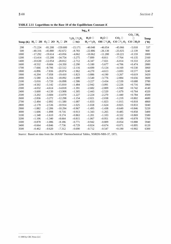
2-68 Section 2
370000000000000000000000000
TABLE 2.11 Logarithms to the Base 10 of the Equilibrium Constant K
log10 K
Temp (K) H2 ⇔ 2H O2 ⇔ 2O N2 ⇔ 2N
1/2O2 + 1/2N2 ⇔NO
H2O ⇔H2 + 1/2O2
H2Ο ⇔OH + 1/2H2
CO2 ⇔CO + 1/2 O2
CO2 + H2 ⇔
CO + H2OTemp (°R)
298 –71.224 –81.208 –159.600 –15.171 –40.048 –46.054 –45.066 –5.018 5500 –40.316 –45.880 –92.672 –8.783 –22.886 –26.130 –25.025 –2.139 90
1000 –17.292 –19.614 –43.056 –4.062 –10.062 –11.280 –10.221 –0.159 181200 –13.414 –15.208 –34.754 –3.275 –7.899 –8.811 –7.764 +0.135 2161400 –10.630 –12.054 –28.812 –2.712 –6.347 –7.021 –6.014 +0.333 2521600 –8.532 –9.684 –24.350 –2.290 –5.180 –5.677 –4.706 +0.474 2881700 –7.666 –8.706 –22.512 –2.116 –4.699 –5.124 –4.169 +0.530 3061800 –6.896 –7.836 –20.874 –1.962 –4.270 –4.613 –3.693 +0.577 3241900 –6.204 –7.058 –19.410 –1.823 –3.886 –4.190 –3.267 +0.619 3422000 –5.580 –6.356 –18.092 –1.699 –3.540 –3.776 –2.884 +0.656 3602100 –5.016 –5.720 –16.898 –1.586 –3.227 –3.434 –2.539 +0.688 3782200 –4.502 –5.142 –15.810 –1.484 –2.942 –3.091 –2.226 +0.716 3962300 –4.032 –4.614 –14.818 –1.391 –2.682 –2.809 –1.940 +0.742 4142400 –3.600 –4.130 –13.908 –1.305 –2.443 –2.520 –1.679 +0.764 4322500 –3.202 –3.684 –13.070 –1.227 –2.224 –2.270 –1.440 +0.784 4502600 –2.836 –3.272 –12.298 –1.154 –2.021 –2.038 –1.219 +0.802 4682700 –2.494 –2.892 –11.580 –1.087 –1.833 –1.823 –1.015 +0.818 4862800 –2.178 –2.536 –10.914 –1.025 –1.658 –1.624 –0.825 +0.833 5042900 –1.882 –2.206 –10.294 –0.967 –1.495 –1.438 –0.649 +0.846 5223000 –1.606 –1.898 –9.716 –0.913 –1.343 –1.265 –0.485 +0.858 5403100 –1.348 –1.610 –9.174 –0.863 –1.201 –1.103 –0.332 +0.869 5583200 –1.106 –1.340 –8.664 –0.815 –1.067 –0.951 –0.189 +0.878 5763300 –0.878 –1.086 –8.186 –0.771 –0.942 –0.809 –0.054 +0.888 5943400 –0.664 –0.846 –7.736 –0.729 –0.824 –0.674 +0.071 +0.895 6123500 –0.462 –0.620 –7.312 –0.690 –0.712 –0.547 +0.190 +0.902 630
Source:Based on data from the JANAF Thermochemical Tables, NSRDS-NBS-37, 1971.
© 1999 by CRC Press LLC
Engineering Thermodynamics 2-69
n,an
ite
structionh
i-
esle
ther
2.5 Exergy Analysis
The method of exergy analysis (availability analysis) presented in this section enables the locatiocause, and true magnitude of energy resource waste and loss to be determined. Such information cbe used in the design of new energy-efficient systems and for improving the performance of existingsystems. Exergy analysis also provides insights that elude a purely first-law approach. For example, onthe basis of first-law reasoning alone, the condenser of a power plant may be mistakenly identified asthe component primarily responsible for the plant’s seemingly low overall performance. An exergyanalysis correctly reveals not only that the condenser loss is relatively unimportant (see the last tworows of the Rankine cycle values of Table 2.15), but also that the steam generator is the principal sof thermodynamic inefficiency owing to combustion and heat transfer irreversibilities within it.
When exergy concepts are combined with principles of engineering economy, the result is known asthermoeconomics. Thermoeconomics allows the real cost sources at the component level to be identified:capital investment costs, operating and maintenance costs, and the costs associated with the deand loss of exergy. Optimization of thermal systems can be achieved by a careful consideration of succost sources. From this perspective thermoeconomics is exergy-aided cost minimization.
Discussions of exergy analysis and thermoeconomics are provided by Bejan et al. (1996), Moran(1989), and Moran and Shapiro (1995). In this section salient aspects are presented.
Defining Exergy
An opportunity for doing work exists whenever two systems at different states are placed in communcation because, in principle, work can be developed as the two are allowed to come into equilibrium.When one of the two systems is a suitably idealized system called an environment and the other is somesystem of interest, exergy is the maximum theoretical useful work (shaft work or electrical work)obtainable as the systems interact to equilibrium, heat transfer occurring with the environment only.(Alternatively, exergy is the minimum theoretical useful work required to form a quantity of matter fromsubstances present in the environment and to bring the matter to a specified state.) Exergy is a measureof the departure of the state of the system from that of the environment, and is therefore an attribute ofthe system and environment together. Once the environment is specified, however, a value can be assignedto exergy in terms of property values for the system only, so exergy can be regarded as an extensiveproperty of the system.
Exergy can be destroyed and generally is not conserved. A limiting case is when exergy would becompletely destroyed, as would occur if a system were to come into equilibrium with the environmentspontaneously with no provision to obtain work. The capability to develop work that existed initiallywould be completely wasted in the spontaneous process. Moreover, since no work needs to be done toeffect such a spontaneous change, the value of exergy can never be negative.
Environment
Models with various levels of specificity are employed for describing the environment used to evaluateexergy. Models of the environment typically refer to some portion of a system’s surroundings, theintensive properties of each phase of which are uniform and do not change significantly as a result ofany process under consideration. The environment is regarded as composed of common substancexisting in abundance within the Earth’s atmosphere, oceans, and crust. The substances are in their stabforms as they exist naturally, and there is no possibility of developing work from interactions — physicalor chemical — between parts of the environment. Although the intensive properties of the environmentare assumed to be unchanging, the extensive properties can change as a result of interactions with osystems. Kinetic and potential energies are evaluated relative to coordinates in the environment, all partsof which are considered to be at rest with respect to one another.
For computational ease, the temperature T0 and pressure p0 of the environment are often taken asstandard-state values, such as 1 atm and 25°C (77°F). However, these properties may be specified
© 1999 by CRC Press LLC
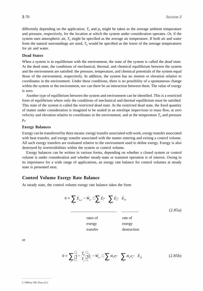
2-70 Section 2
urer, if theaterres
systemem equaltive to change exergy
trictedsfied.ty at zero
sociatedolume. is also
controlwing tosteady
differently depending on the application. T0 and p0 might be taken as the average ambient temperatand pressure, respectively, for the location at which the system under consideration operates. Osystem uses atmospheric air, T0 might be specified as the average air temperature. If both air and wfrom the natural surroundings are used, T0 would be specified as the lower of the average temperatufor air and water.
Dead States
When a system is in equilibrium with the environment, the state of the system is called the dead state.At the dead state, the conditions of mechanical, thermal, and chemical equilibrium between the and the environment are satisfied: the pressure, temperature, and chemical potentials of the systthose of the environment, respectively. In addition, the system has no motion or elevation relacoordinates in the environment. Under these conditions, there is no possibility of a spontaneouswithin the system or the environment, nor can there be an interaction between them. The value ofis zero.
Another type of equilibrium between the system and environment can be identified. This is a resform of equilibrium where only the conditions of mechanical and thermal equilibrium must be satiThis state of the system is called the restricted dead state. At the restricted dead state, the fixed quantiof matter under consideration is imagined to be sealed in an envelope impervious to mass flow,velocity and elevation relative to coordinates in the environment, and at the temperature T0 and pressurep0.
Exergy Balances
Exergy can be transferred by three means: exergy transfer associated with work, exergy transfer aswith heat transfer, and exergy transfer associated with the matter entering and exiting a control vAll such exergy transfers are evaluated relative to the environment used to define exergy. Exergydestroyed by irreversibilities within the system or control volume.
Exergy balances can be written in various forms, depending on whether a closed system or volume is under consideration and whether steady-state or transient operation is of interest. Oits importance for a wide range of applications, an exergy rate balance for control volumes at state is presented next.
Control Volume Exergy Rate Balance
At steady state, the control volume exergy rate balance takes the form
(2.85a)
or
(2.85b)
0 = − + − −∑ ∑ ∑˙ ˙ ˙ ˙ ˙
________________________ _________
,E W E E Eq j cv
j
i
i
e
e
D
rates of
exergy
transfer
rate of
exergy
destruction
0 1 0= −
− + − −∑ ∑ ∑T
TQ W m e m e E
jj
j cv i i
i
e e
e
D˙ ˙ ˙ ˙ ˙
© 1999 by CRC Press LLC
Engineering Thermodynamics 2-71
is theaneous
y.and
thin
cal
rictedes
hemicalreferredernative89) and
f the
standardnt. There, solidhemical, called
ciples,t that
has the same significance as in Equation 2.22: the work rate excluding the flow work. time rate of heat transfer at the location on the boundary of the control volume where the instanttemperature is Tj. The associated rate of exergy transfer is
(2.86)
As for other control volume rate balances, the subscripts i and e denote inlets and outlets, respectivelThe exergy transfer rates at control volume inlets and outlets are denoted, respectively, as
Finally, accounts for the time rate of exergy destruction due to irreversibilities withe control volume. The exergy destruction rate is related to the entropy generation rate by
(2.87)
The specific exergy transfer terms ei and ee are expressible in terms of four components: physiexergy ePH, kinetic exergy eKN, potential exergy ePT, and chemical exergy eCH:
(2.88)
The first three components are evaluated as follows:
(2.89a)
(2.89b)
(2.89c)
In Equation 2.89a, h0 and s0 denote, respectively, the specific enthalpy and specific entropy at the restdead state. In Equations 2.89b and 2.89c, v and z denote velocity and elevation relative to coordinatin the environment, respectively. The chemical exergy eCH is considered next.
Chemical Exergy
To evaluate the chemical exergy, the exergy component associated with the departure of the ccomposition of a system from that of the environment, the substances comprising the system are to the properties of a suitably selected set of environmental substances. For this purpose, altmodels of the environment have been developed. For discussion, see, for example, Moran (19Kotas (1995).
Exergy analysis is facilitated, however, by employing a standard environment and a correspondingtable of standard chemical exergies. Standard chemical exergies are based on standard values oenvironmental temperature T0 and pressure p0 — for example, 298.15 K (25°C) and 1 atm, respectively.A standard environment is also regarded as consisting of a set of reference substances with concentrations reflecting as closely as possible the chemical makeup of the natural environmereference substances generally fall into three groups: gaseous components of the atmosphesubstances from the lithosphere, and ionic and noninonic substances from the oceans. The cexergy data of Table 2.12 correspond to two alternative standard exergy reference environmentshere model I and model II, that have gained acceptance for engineering evaluations.
Although the use of standard chemical exergies greatly facilitates the application of exergy printhe term standard is somewhat misleading since there is no one specification of the environmen
Wcv Qj
˙ ˙,E
T
TQq j
jj= −
1 0
˙ ˙E m ei i i=˙ ˙ .E m ee e e= ED
˙ ˙E T SD gen= 0
e e e e ePH KN PT CH= + + +
e h h T s sPH = −( ) − −( )0 0 0
eKN = 12
v2
e gzPT =
© 1999 by CRC Press LLC
2-72 Section 2
he
f
suffices for all applications. Still, chemical exergies calculated relative to alternative specifications ofthe environment are generally in good agreement. For a broad range of engineering applications tsimplicity and ease of use of standard chemical exergies generally outweigh any slight lack of accuracythat might result. In particular, the effect of slight variations in the values of T0 and p0 about the valuesused to determine the standard chemical exergies reported in Table 2.12 can be neglected.
The literature of exergy analysis provides several expressions allowing the chemical exergy to beevaluated in particular cases of interest. The molar chemical exergy of a gas mixture, for example, canbe evaluated from
(2.90)
where is the molar chemical exergy of the ith component.
Example 13
Ignoring the kinetic and potential exergies, determine the exergy rate, in kJ/kg, associated with each othe following streams of matter:
(a) Saturated water vapor at 20 bar.(b) Methane at 5 bar, 25°C.
Let T0 = 298 K, p0 = 1.013 bar (1 atm).
Solution. Equation 2.88 reduces to read
(a) From Table A.5, h = 2799.5 kJ/kg, s = 6.3409 kJ/kg · K. At T0 = 298 K (25°C), water would bea liquid; thus with Equations 2.50c and 2.50d, h0 ≈ 104.9 kJ/kg, s0 ≈ 0.3674 kJ/kg · K. Table 2.12(model I) gives eCH = 45/18.02 = 2.5 kJ/kg. Then
Here the specific exergy is determined predominately by the physical component.(b) Assuming the ideal gas model for methane, h – h0 = 0. Also, Equation 2.58 reduces to give s –
s0 = –Rlnp/p0. Then, Equation 2.88 reads
With eCH = 824,350/16.04 = 51,393.4 kJ/kg from Table 2.12 (model I),
Here the specific exergy is determined predominately by the chemical component.
e y e RT y yCHi i
CH
i
j
i i
i
j
= += =
∑ ∑1
0
1
ln
eiCH
e h h T s s eCH= −( ) − −( ) +0 0 0
e = −( ) − −( ) +
= + =
2799 5 104 9 298 6 3409 0 3674 2 5
914 5 2 5 917 0
. . . . .
. . . kJ kg
e RT p p eCH= +0 0ln
e =⋅
( ) +
= +
=
8 31416 04
51 013
51 393 4
246 6 51 393 4
..
ln.
, .
. , .
kJkg K
298 KkJkg
51,640 kJ kg
© 1999 by CRC Press LLC
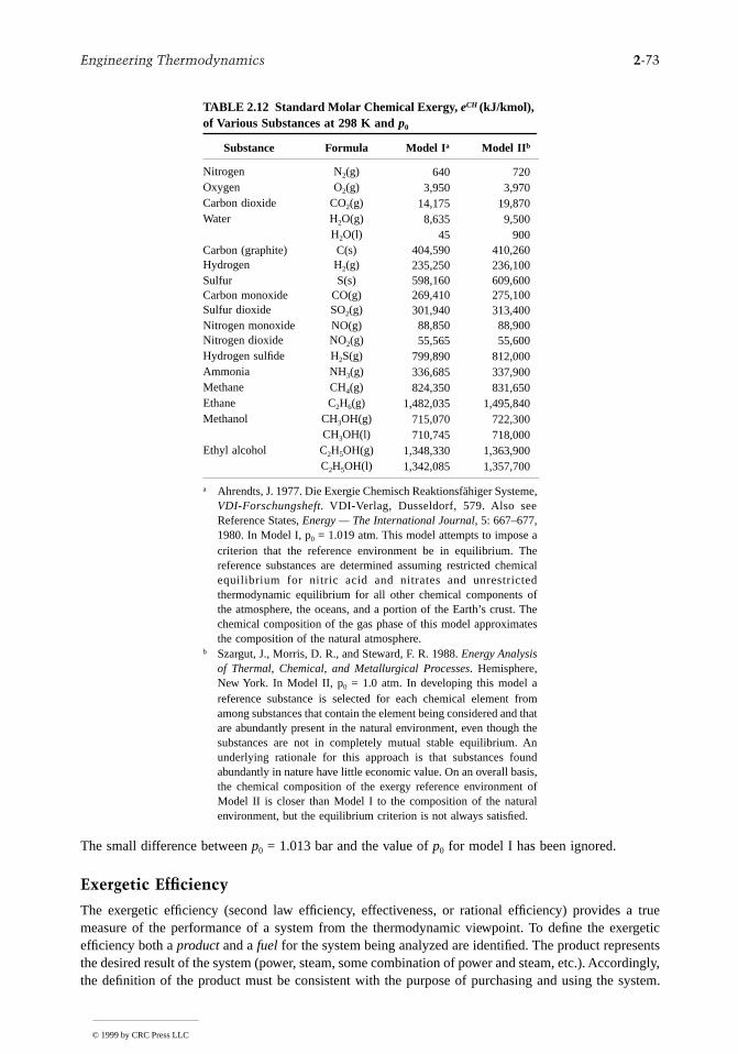
Engineering Thermodynamics 2-73
trueergeticentsrdingly,ystem.
The small difference between p0 = 1.013 bar and the value of p0 for model I has been ignored.
Exergetic Efficiency
The exergetic efficiency (second law efficiency, effectiveness, or rational efficiency) provides ameasure of the performance of a system from the thermodynamic viewpoint. To define the exefficiency both a product and a fuel for the system being analyzed are identified. The product represthe desired result of the system (power, steam, some combination of power and steam, etc.). Accothe definition of the product must be consistent with the purpose of purchasing and using the s
TABLE 2.12 Standard Molar Chemical Exergy, eCH (kJ/kmol), of Various Substances at 298 K and p0
Substance Formula Model Ia Model II b
Nitrogen N2(g) 640 720Oxygen O2(g) 3,950 3,970Carbon dioxide CO2(g) 14,175 19,870Water H2O(g) 8,635 9,500
H2O(l) 45 900Carbon (graphite) C(s) 404,590 410,260Hydrogen H2(g) 235,250 236,100Sulfur S(s) 598,160 609,600Carbon monoxide CO(g) 269,410 275,100Sulfur dioxide SO2(g) 301,940 313,400Nitrogen monoxide NO(g) 88,850 88,900Nitrogen dioxide NO2(g) 55,565 55,600Hydrogen sulfide H2S(g) 799,890 812,000Ammonia NH3(g) 336,685 337,900Methane CH4(g) 824,350 831,650Ethane C2H6(g) 1,482,035 1,495,840Methanol CH3OH(g) 715,070 722,300
CH3OH(l) 710,745 718,000Ethyl alcohol C2H5OH(g) 1,348,330 1,363,900
C2H5OH(l) 1,342,085 1,357,700
a Ahrendts, J. 1977. Die Exergie Chemisch Reaktionsfähiger Systeme,VDI-Forschungsheft. VDI-Verlag, Dusseldorf, 579. Also seeReference States, Energy — The International Journal, 5: 667–677,1980. In Model I, p0 = 1.019 atm. This model attempts to impose acriterion that the reference environment be in equilibrium. Thereference substances are determined assuming restricted chemicalequilibrium for nitric acid and nitrates and unrestrictedthermodynamic equilibrium for all other chemical components ofthe atmosphere, the oceans, and a portion of the Earth’s crust. Thechemical composition of the gas phase of this model approximatesthe composition of the natural atmosphere.
b Szargut, J., Morris, D. R., and Steward, F. R. 1988. Energy Analysisof Thermal, Chemical, and Metallurgical Processes. Hemisphere,New York. In Model II, p0 = 1.0 atm. In developing this model areference substance is selected for each chemical element fromamong substances that contain the element being considered and thatare abundantly present in the natural environment, even though thesubstances are not in completely mutual stable equilibrium. Anunderlying rationale for this approach is that substances foundabundantly in nature have little economic value. On an overall basis,the chemical composition of the exergy reference environment ofModel II is closer than Model I to the composition of the naturalenvironment, but the equilibrium criterion is not always satisfied.
© 1999 by CRC Press LLC
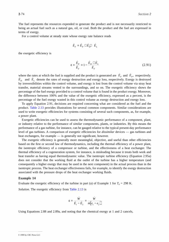
2-74 Section 2
d to
e
and there
, plant,thee
andhe
The fuel represents the resources expended to generate the product and is not necessarily restrictebeing an actual fuel such as a natural gas, oil, or coal. Both the product and the fuel are expressed interms of exergy.
For a control volume at steady state whose exergy rate balance reads
the exergetic efficiency is
(2.91)
where the rates at which the fuel is supplied and the product is generated are and respectively. and denote the rates of exergy destruction and exergy loss, respectively. Exergy is destroyed
by irreversibilities within the control volume, and exergy is lost from the control volume via stray heattransfer, material streams vented to the surroundings, and so on. The exergetic efficiency shows thepercentage of the fuel exergy provided to a control volume that is found in the product exergy. Moreover,the difference between 100% and the value of the exergetic efficiency, expressed as a percent, is thpercentage of the fuel exergy wasted in this control volume as exergy destruction and exergy loss.
To apply Equation 2.91, decisions are required concerning what are considered as the fuel product. Table 2.13 provides illustrations for several common components. Similar considerations aused to write exergetic efficiencies for systems consisting of several such components, as, for example,a power plant.
Exergetic efficiencies can be used to assess the thermodynamic performance of a componentor industry relative to the performance of similar components, plants, or industries. By this means performance of a gas turbine, for instance, can be gauged relative to the typical present-day performanclevel of gas turbines. A comparison of exergetic efficiencies for dissimilar devices — gas turbines andheat exchangers, for example — is generally not significant, however.
The exergetic efficiency is generally more meaningful, objective, and useful than other efficienciesbased on the first or second law of thermodynamics, including the thermal efficiency of a power plant,the isentropic efficiency of a compressor or turbine, and the effectiveness of a heat exchanger. Thethermal efficiency of a cogeneration system, for instance, is misleading because it treats both work andheat transfer as having equal thermodynamic value. The isentropic turbine efficiency (Equation 2.95a)does not consider that the working fluid at the outlet of the turbine has a higher temperature (consequently a higher exergy that may be used in the next component) in the actual process than in tisentropic process. The heat exchanger effectiveness fails, for example, to identify the exergy destructionassociated with the pressure drops of the heat exchanger working fluids.
Example 14
Evaluate the exergetic efficiency of the turbine in part (a) of Example 1 for T0 = 298 K.
Solution. The exergetic efficiency from Table 2.13 is
Using Equations 2.88 and 2.89a, and noting that the chemical exergy at 1 and 2 cancels,
˙ ˙ ˙ ˙E E E EF P D L= + +
ε = = −+˙
˙
˙ ˙
˙E
E
E E
EP
F
D L
F
1
EF˙ ,EP
ED EL
ε =−
=−( )
˙
˙ ˙
˙
˙W
E E
W
m e e1 2 1 2
© 1999 by CRC Press LLC
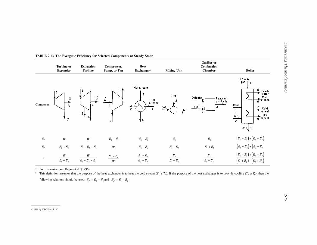
En
gineerin
g Th
ermod
ynam
ics
2
-75
© 1998 by CRC Pres
TABLE 2.1
GasiÞer orCombustion
Chamber Boiler
Component
e
a
For discu
b
This deÞn
e heat exchanger is to provide cooling (
T
3
³
T
0
), then the
following
ÇEPÇE3
Ç Ç Ç ÇE E E E6 5 8 7-( ) + -( )ÇEF
Ç ÇE E1 2+ Ç Ç Ç ÇE E E E1 2 3 4+( ) + +( )Ç
Ç ÇE
E E3
1 2+
Ç Ç Ç Ç
Ç Ç Ç Ç
E E E E
E E E E
6 5 8 7
1 2 3 4
-( ) + -( )+( ) - +( )
s LLC
3 The Exergetic EfÞciency for Selected Components at Steady Statea
Turbine orExpander
ExtractionTurbine
Compressor,Pump, or Fan
HeatExchangerb Mixing Unit
ssion, see Bejan et al. (1996).ition assumes that the purpose of the heat exchanger is to heat the cold stream (T1 ³ T0). If the purpose of th
relations should be used: and
ÇW ÇW Ç ÇE E2 1- Ç ÇE E2 1- ÇE3
Ç ÇE E1 2- Ç Ç ÇE E E1 2 3- - ÇW Ç ÇE E3 4- Ç ÇE E1 2+
Ç
Ç ÇW
E E1 2-
Ç
Ç Ç ÇW
E E E1 2 3- -
Ç Ç
ÇE E
W2 1-
Ç Ç
Ç ÇE E
E E2 1
3 4
-
-
Ç
Ç ÇE
E E3
1 2+
Ç Ç ÇE E EP = -4 3Ç Ç Ç .E E EF = -1 2
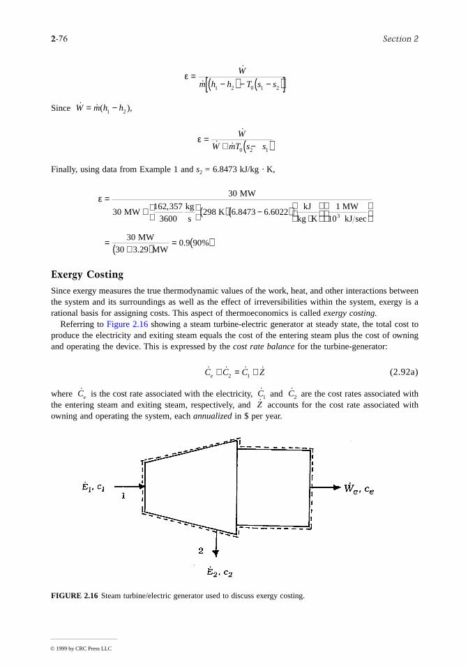
2-76 Section 2
n
st to
thith
Since
Finally, using data from Example 1 and
s
2
= 6.8473 kJ/kg · K,
Exergy Costing
Since exergy measures the true thermodynamic values of the work, heat, and other interactions betweethe system and its surroundings as well as the effect of irreversibilities within the system, exergy is arational basis for assigning costs. This aspect of thermoeconomics is called
exergy costing.
Referring to Figure 2.16 showing a steam turbine-electric generator at steady state, the total coproduce the electricity and exiting steam equals the cost of the entering steam plus the cost of owningand operating the device. This is expressed by the
cost rate balance
for the turbine-generator:
(2.92a)
where is the cost rate associated with the electricity, and are the cost rates associated withe entering steam and exiting steam, respectively, and accounts for the cost rate associated wowning and operating the system, each
annualized
in $ per year.
FIGURE 2.16
Steam turbine/electric generator used to discuss exergy costing.
ε =−( ) − −( )[ ]
˙
˙
W
m h h T s s1 2 0 1 2
˙ ˙ ( ),W m h h= −1 2
ε =+ −( )
˙
˙ ˙W
W mT s s0 2 1
ε =+
( ) −( )
⋅
=+( )
= ( )
30
30162 357
3600298 6 8473 6 6022
3030 3 29
0 9 90
MW
MWkgs
KkJ
kg K1 MW
10 kJ sec
MWMW
3
,. .
.. %
˙ ˙ ˙ ˙C C C Ze + = +2 1
Ce C1 C2
Z
© 1999 by CRC Press LLC
Engineering Thermodynamics 2-77
of
ll costs
ts
With exergy costing, the cost rates and are evaluated in terms of the associated rate exergy transfer and a
unit cost.
Equation 2.92a then appears as
(2.92b)
The coefficients
c
1
,
c
2
, and
c
e
in Equation 2.92b denote the
average
cost per unit of exergy for theassociated exergy rate. The unit cost
c
1
of the entering steam would be obtained from exergy costingapplied to the components upstream of the turbine. Assigning the same unit cost to the exiting steam:
c
2
=
c
1
on the basis that the purpose of the turbine-generator is to generate electricity and thus aassociated with owning and operating the system should be charged to the power, Equation 2.92b becomes
(2.92c)
The first term on the right side accounts for the cost of the net exergy used and the second term accounfor cost of the system itself. Introducing the exergetic efficiency from Table 2.13, the unit cost of theelectricity is
(2.93)
This equation shows, for example, that the unit cost of electricity would increase if the exergetic efficiencywere to decrease owing to a deterioration of the turbine with use.
Example 15
A turbine-generator with an exergetic efficiency of 90% develops 7
×
10
7
kW · hr of electricity annually.The annual cost of owning and operating the system is $2.5
×
10
5
. If the average unit cost of the steamentering the system is $0.0165 per kW · hr of exergy, evaluate the unit cost of the electricity.
Solution.
Substituting values into Equation 2.93,
˙ , ˙ ,C C1 2 Ce
c W c E c E Ze e˙ ˙ ˙ ˙+ = +2 2 1 1
c W c E E Ze e˙ ˙ ˙ ˙= −( ) +1 1 2
cc Z
Wee
= +1
ε
˙
˙
ce = ⋅ + ×× ⋅
= + = ⋅
$0.0165 kW h0.9
2.5 10 year7 10 kW h year
$0.0219 kW h
5
7
$
. .0 0183 0 0036
© 1999 by CRC Press LLC
2-78 Section 2
nt
e-
also
eal
e
s of
jection
2.6 Vapor and Gas Power Cycles
Vapor and gas power systems develop electrical or mechanical power from energy sources of chemical,solar, or nuclear origin. In
vapor
power systems the
working fluid
,
normally water, undergoes a phasechange from liquid to vapor, and conversely. In
gas
power systems, the working fluid remains a gasthroughout, although the composition normally varies owing to the introduction of a fuel and subsequecombustion. The present section introduces vapor and gas power systems. Further discussion is providedin Chapter 8. Refrigeration systems are considered in Chapter 9.
The processes taking place in power systems are sufficiently complicated that idealizations aretypically employed to develop tractable thermodynamic models. The
air standard analysis
of gas powersystems considered later in the present section is a noteworthy example. Depending on the degree ofidealization, such models may provide only qualitative information about the performance of the corrsponding real-world systems. Yet such information is frequently useful in gauging how changes in majoroperating parameters might affect actual performance. Elementary thermodynamic models can provide simple settings to assess, at least approximately, the advantages and disadvantages of featuresproposed to improve thermodynamic performance.
Rankine and Brayton Cycles
In their simplest embodiments vapor power and gas turbine power plants are represented conventionallyin terms of four components in series, forming, respectively, the Rankine
cycle and the Brayton
cycleshown schematically in Table 2.14. The thermodynamically ideal counterparts of these cycles arecomposed of four internally reversible processes in series: two isentropic processes alternated with twoconstant pressure processes. Table 2.14 provides property diagrams of the actual and corresponding idcycles. Each actual cycle is denoted 1-2-3-4-1; the ideal cycle is 1-2s-3-4s-1. For simplicity, pressuredrops through the boiler, condenser, and heat exchangers are not shown. Invoking Equation 2.29 for theideal cycles, the heat added per unit of mass flowing is represented by the area
under
the isobar fromstate 2s to state 3: area a-2s-3-b-a. The heat rejected is the area
under
the isobar from state 4s to stat1: area a-1-4s-b-a. Enclosed area 1-2s-3-4s-1 represents the net heat added per unit of massflowing.For any power cycle, the net heat added equals the net work done.
Expressions for the principal energy transfers shown on the schematics of Table 2.14 are provided byEquations 1 to 4 of the table. They are obtained by reducing Equation 2.27a with the assumptionnegligible heat loss and negligible changes in kinetic and potential energy from the inlet to the outletof each component. All quantities are positive in the directions of the arrows on the figure. Using theseexpressions, the thermal efficiency is
(2.94)
To obtain the thermal efficiency of the ideal cycle,
h
2
s
replaces
h
2
and
h
4
s
replaces
h
4
in Equation 2.94.Decisions concerning cycle operating conditions normally recognize that the thermal efficiency tends
to increase as the average temperature of heat addition increases and/or the temperature of heat redecreases. In the Rankine cycle, a high average temperature of heat addition can be achieved bysuperheating the vapor prior to entering the turbine, and/or by operating at an elevated steam-generatorpressure. In the Brayton cycle an increase in the compressor pressure ratio
p
2
/
p
1
tends to increase theaverage temperature of heat addition. Owing to materials limitations at elevated temperatures andpressures, the state of the working fluid at the turbine inlet must observe practical limits, however. Theturbine inlet temperature of the Brayton cycle, for example, is controlled by providing air far in excessof what is required for combustion. In a Rankine cycle using water as the working fluid, a low temperatureof heat rejection is typically achieved by operating the condenser at a pressure below 1 atm. To reduce
η =−( ) − −( )
−h h h h
h h3 4 2 1
3 2
© 1999 by CRC Press LLC
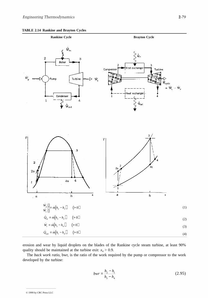
Engineering Thermodynamics 2-79
st 90%
ork
erosion and wear by liquid droplets on the blades of the Rankine cycle steam turbine, at leaquality should be maintained at the turbine exit:
x
4
> 0.9.The
back work ratio
,
bwr, is the ratio of the work required by the pump or compressor to the wdeveloped by the turbine:
(2.95)
TABLE 2.14 Rankine and Brayton Cycles
Rankine Cycle Brayton Cycle
(1)
(2)
(3)
(4)
˙
˙˙
W
Wm h hp
c
= −( ) >( )2 1 0
˙ ˙Q m h hin = −( ) >( )3 2 0
˙ ˙W m h ht = −( ) >( )3 4 0
˙ ˙Q m h hout = −( ) >( )1 4 0
bwrh h
h h=
−−
2 1
3 4
© 1999 by CRC Press LLC
2-80 Section 2
is
r ise
lr
gs
ark
As a relatively high specific volume vapor expands through the turbine of the Rankine cycle and a muchlower specific volume liquid is pumped, the back work ratio is characteristically quite low in vaporpower plants — in many cases on the order of 1 to 2%. In the Brayton cycle, however, both the turbineand compressor handle a relatively high specific volume gas, and the back ratio is much larger, typically40% or more.
The effect of friction and other irreversibilities for flow-through turbines, compressors, and pumpscommonly accounted for by an appropriate
isentropic efficiency.
The isentropic turbine efficiency is
(2.95a)
The isentropic compressor efficiency is
(2.95b)
In the isentropic pump efficiency,
η
p
, which takes the same form as Equation 2.95b, the numeratofrequently approximated via Equation 2.30c
as h
2s
–
h
1
≈
v
1
∆
p
,
where
∆
p
is the pressure rise across thpump.
Simple gas turbine power plants differ from the Brayton cycle model in significant respects. In actuaoperation, excess air is continuously drawn into the compressor, where it is compressed to a highepressure; then fuel is introduced and combustion occurs; finally the mixture of combustion products andair expands through the turbine and is subsequently discharged to the surroundings. Accordingly, thelow-temperature heat exchanger shown by a dashed line in the Brayton cycle schematic of Table 2.14is not an actual component, but included only to account formally for the cooling in the surroundinof the hot gas discharged from the turbine.
Another frequently employed idealization used with gas turbine power plants is that of an air-standardanalysis. An air-standard analysis involves two major assumptions: (1) as shown by the Brayton cycleschematic of Table 2.14, the temperature rise that would be brought about by combustion is effectedinstead by a heat transfer from an external source; (2) the working fluid throughout the cycle is air,which behaves as an ideal gas. In a cold air-standard analysis the specific heat ratio k for air is taken asconstant. Equations 1 to 6 of Table 2.7 together with data from Table A.8 apply generally to air-standardanalyses. Equations 1′ to 6′ of Table 2.7 apply to cold air-standard analyses, as does the followingexpression for the turbine power obtained from Table 2.1 (Equation 27c″):
(2.96)
(Equation 2.96 also corresponds to Equation 5′ of Table 2.8 when n = k.) An expression similar in formcan be written for the power required by the compressor.
For the simple Rankine and Brayton cycles of Table 2.14 the results of sample calculations are providedin Table 2.15. The Brayton cycle calculations are on an air-standard analysis basis.
Otto, Diesel, and Dual Cycles
Although most gas turbines are also internal combustion engines, the name is usually reserved toreciprocating internal combustion engines of the type commonly used in automobiles, trucks, and buses.Two principal types of reciprocating internal combustion engines are the spark-ignition engine and thecompression-ignition engine. In a spark-ignition engine a mixture of fuel and air is ignited by a sp
ηts
h h
h h=
−−
3 4
3 4
ηcsh h
h h=
−−
2 1
2 1
˙ ˙W mkRT
kp pt
k k=
−− ( )[ ]−( )3
4 3
1
11
© 1999 by CRC Press LLC
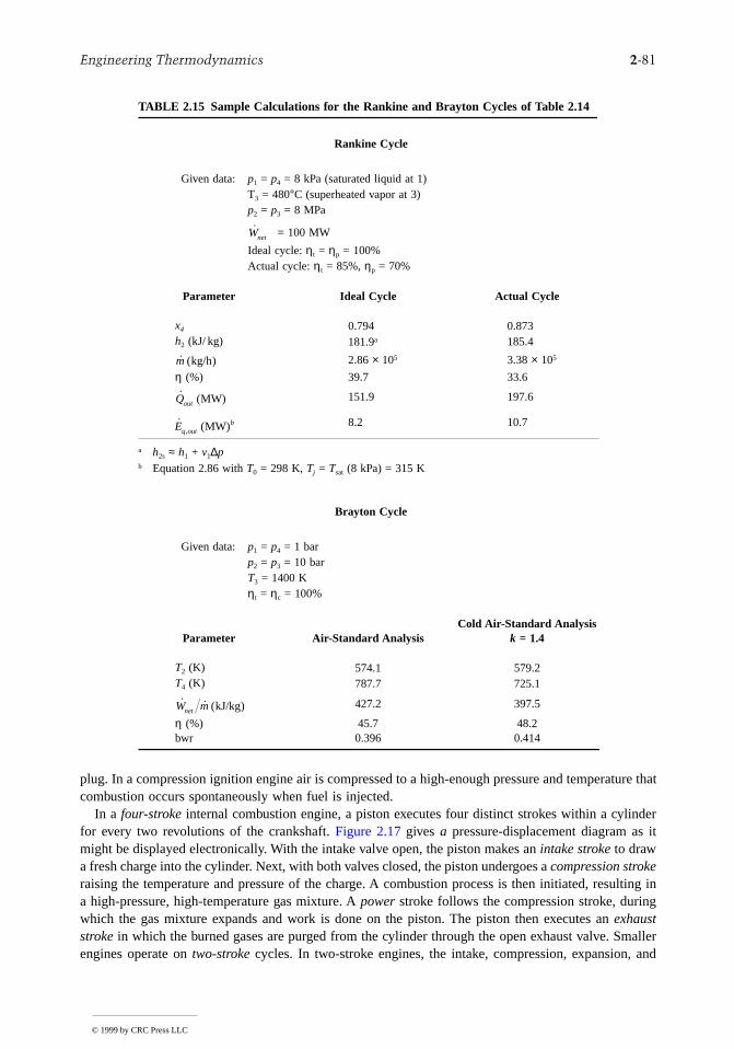
Engineering Thermodynamics
2
-81
ture that
it
n
plug. In a compression ignition engine air is compressed to a high-enough pressure and temperacombustion occurs spontaneously when fuel is injected.
In a four-stroke internal combustion engine, a piston executes four distinct strokes within a cylinderfor every two revolutions of the crankshaft. Figure 2.17 gives a pressure-displacement diagram as might be displayed electronically. With the intake valve open, the piston makes an intake stroke to drawa fresh charge into the cylinder. Next, with both valves closed, the piston undergoes a compression strokeraising the temperature and pressure of the charge. A combustion process is then initiated, resulting ia high-pressure, high-temperature gas mixture. A power stroke follows the compression stroke, duringwhich the gas mixture expands and work is done on the piston. The piston then executes an exhauststroke in which the burned gases are purged from the cylinder through the open exhaust valve. Smallerengines operate on two-stroke cycles. In two-stroke engines, the intake, compression, expansion, and
TABLE 2.15 Sample Calculations for the Rankine and Brayton Cycles of Table 2.14
Rankine Cycle
Given data: p1 = p4 = 8 kPa (saturated liquid at 1)T3 = 480°C (superheated vapor at 3)p2 = p3 = 8 MPa
= 100 MW
Ideal cycle: ηt = ηp = 100%Actual cycle: ηt = 85%, ηp = 70%
Parameter Ideal Cycle Actual Cycle
x4 0.794 0.873h2 (kJ/ kg) 181.9a 185.4
2.86 × 10⁵ 3.38 × 10⁵
η (%) 39.7 33.6
151.9 197.6
8.2 10.7
a h2s ≈ h1 + v1∆pb Equation 2.86 with T0 = 298 K, Tj = Tsat (8 kPa) = 315 K
Brayton Cycle
Given data: p1 = p4 = 1 barp2 = p3 = 10 barT3 = 1400 Kηt = ηc = 100%
Parameter Ai r-Standard AnalysisCold Air-Standard Analysis
k = 1.4
T2 (K) 574.1 579.2T4 (K) 787.7 725.1
427.2 397.5
η (%) 45.7 48.2bwr 0.396 0.414
Wnet
˙ ( )m kg/h
˙ (Qout MW)
˙ (,Eq outbMW)
˙ ˙ ( )W mnet kJ/kg
© 1999 by CRC Press LLC
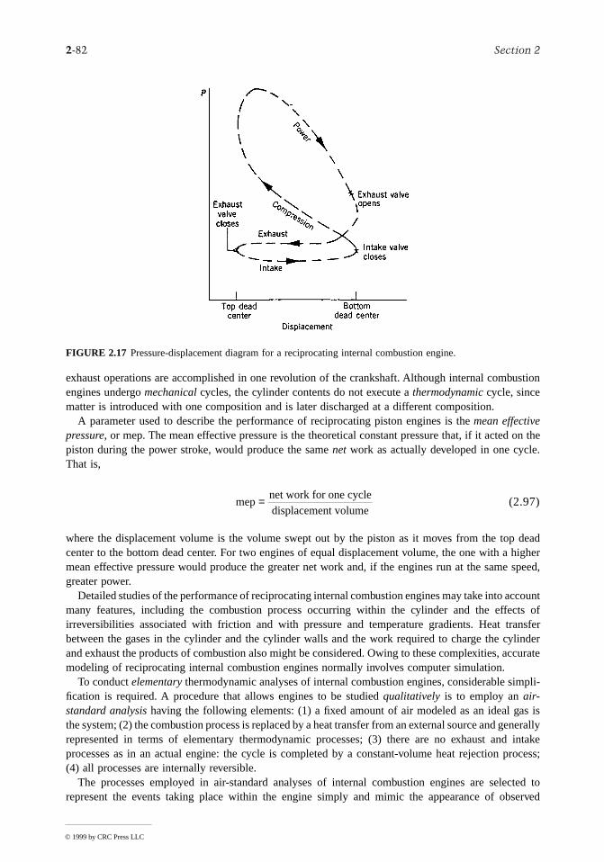
2-82 Section 2
ustion
on the.
p dead higher
e speed,
ccountcts ofansferylinderccurate
mpli-
as isgenerallyd intakeprocess;
cted toserved
exhaust operations are accomplished in one revolution of the crankshaft. Although internal combengines undergo mechanical cycles, the cylinder contents do not execute a thermodynamic cycle, sincematter is introduced with one composition and is later discharged at a different composition.
A parameter used to describe the performance of reciprocating piston engines is the mean effectivepressure, or mep. The mean effective pressure is the theoretical constant pressure that, if it actedpiston during the power stroke, would produce the same net work as actually developed in one cycleThat is,
(2.97)
where the displacement volume is the volume swept out by the piston as it moves from the tocenter to the bottom dead center. For two engines of equal displacement volume, the one with amean effective pressure would produce the greater net work and, if the engines run at the samgreater power.
Detailed studies of the performance of reciprocating internal combustion engines may take into amany features, including the combustion process occurring within the cylinder and the effeirreversibilities associated with friction and with pressure and temperature gradients. Heat trbetween the gases in the cylinder and the cylinder walls and the work required to charge the cand exhaust the products of combustion also might be considered. Owing to these complexities, amodeling of reciprocating internal combustion engines normally involves computer simulation.
To conduct elementary thermodynamic analyses of internal combustion engines, considerable sification is required. A procedure that allows engines to be studied qualitatively is to employ an air-standard analysis having the following elements: (1) a fixed amount of air modeled as an ideal gthe system; (2) the combustion process is replaced by a heat transfer from an external source and represented in terms of elementary thermodynamic processes; (3) there are no exhaust anprocesses as in an actual engine: the cycle is completed by a constant-volume heat rejection (4) all processes are internally reversible.
The processes employed in air-standard analyses of internal combustion engines are selerepresent the events taking place within the engine simply and mimic the appearance of ob
FIGURE 2.17 Pressure-displacement diagram for a reciprocating internal combustion engine.
mepnet work for one cycledisplacement volume
=
© 1999 by CRC Press LLC
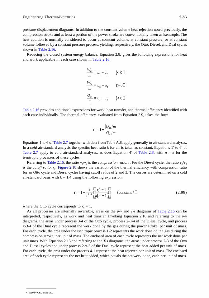
Engineering Thermodynamics 2-83
nt
ttoss.
.
pressure-displacement diagrams. In addition to the constant volume heat rejection noted previously, thecompression stroke and at least a portion of the power stroke are conventionally taken as isentropic. Theheat addition is normally considered to occur at constant volume, at constant pressure, or at constavolume followed by a constant pressure process, yielding, respectively, the Otto, Diesel, and Dual cyclesshown in Table 2.16.
Reducing the closed system energy balance, Equation 2.8, gives the following expressions for heatand work applicable in each case shown in Table 2.16:
Table 2.16 provides additional expressions for work, heat transfer, and thermal efficiency identified witheach case individually. The thermal efficiency, evaluated from Equation 2.9, takes the form
Equations 1 to 6 of Table 2.7 together with data from Table A.8, apply generally to air-standard analyses.In a cold air-standard analysis the specific heat ratio k for air is taken as constant. Equations 1′ to 6′ ofTable 2.7 apply to cold air-standard analyses, as does Equation 4′ of Table 2.8, with n = k for theisentropic processes of these cycles.
Referring to Table 2.16, the ratio v1/v2 is the compression ratio, r. For the Diesel cycle, the ratio v3/v2
is the cutoff ratio, rc. Figure 2.18 shows the variation of the thermal efficiency with compression ratiofor an Otto cycle and Diesel cycles having cutoff ratios of 2 and 3. The curves are determined on a coldair-standard basis with k = 1.4 using the following expression:
(2.98)
where the Otto cycle corresponds to rc = 1.As all processes are internally reversible, areas on the p-v and T-s diagrams of Table 2.16 can be
interpreted, respectively, as work and heat transfer. Invoking Equation 2.10 and referring to the p-vdiagrams, the areas under process 3-4 of the Otto cycle, process 2-3-4 of the Diesel cycle, and processx-3-4 of the Dual cycle represent the work done by the gas during the power stroke, per unit of mass.For each cycle, the area under the isentropic process 1-2 represents the work done on the gas during thecompression stroke, per unit of mass. The enclosed area of each cycle represents the net work done perunit mass. With Equation 2.15 and referring to the T-s diagrams, the areas under process 2-3 of the Oand Diesel cycles and under process 2-x-3 of the Dual cycle represent the heat added per unit of maFor each cycle, the area under the process 4-1 represent the heat rejected per unit of mass. The enclosedarea of each cycle represents the net heat added, which equals the net work done, each per unit of mass
W
mu u
W
mu u
Q
mu u
121 2
343 4
411 4
0
0
0
= − <( )
= − >( )
= − <( )
η = −1 41Q m
Q mA
η = −−−( )
( )−11 1
11r
r
k rkk
ck
c
constant
© 1999 by CRC Press LLC
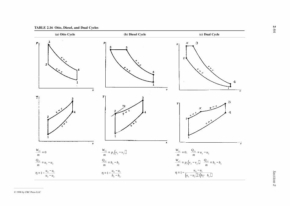
2
-84
Section 2
©
(c) Dual Cycle
Q
mu ux
x2
20 = −,
p v vQ
mh hx
x3 3 23
3−( ) = −,
−−( ) + −( )
4 1
2 3
u u
u u h hx x
1998 by CRC Press LLC
TABLE 2.16 Otto, Diesel, and Dual Cycles
(a) Otto Cycle (b) Diesel Cycle
W
m23 0=
W
mp v v232 3 2= −( ) W
mx2 =
Q
mu u233 2= −
Q
mh h233 2= −
W
mx3 =
η = −−−
1 4 1
3 2
u u
u uη = −
−−
1 4 1
3 2
u u
h hη = −1
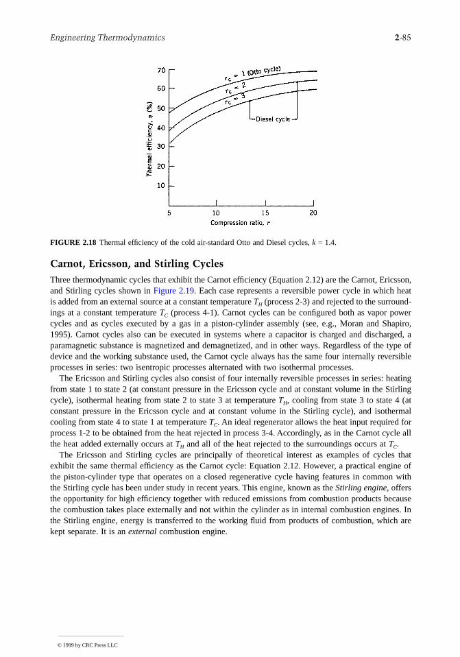
Engineering Thermodynamics 2-85
n,
d-
ro,
g
t
Carnot, Ericsson, and Stirling Cycles
Three thermodynamic cycles that exhibit the Carnot efficiency (Equation 2.12) are the Carnot, Ericssoand Stirling cycles shown in Figure 2.19. Each case represents a reversible power cycle in which heatis added from an external source at a constant temperature
T
H
(process 2-3) and rejected to the surrounings at a constant temperature
T
C
(process 4-1). Carnot cycles can be configured both as vapor powercycles and as cycles executed by a gas in a piston-cylinder assembly (see, e.g., Moran and Shapi1995). Carnot cycles also can be executed in systems where a capacitor is charged and discharged, aparamagnetic substance is magnetized and demagnetized, and in other ways. Regardless of the type ofdevice and the working substance used, the Carnot cycle always has the same four internally reversibleprocesses in series: two isentropic processes alternated with two isothermal processes.
The Ericsson and Stirling cycles also consist of four internally reversible processes in series: heatinfrom state 1 to state 2 (at constant pressure in the Ericsson cycle and at constant volume in the Stirlingcycle), isothermal heating from state 2 to state 3 at temperature
T
H
, cooling from state 3 to state 4 (a
constant pressure in the Ericsson cycle and at constant volume in the Stirling cycle), and isothermalcooling from state 4 to state 1 at temperature
T
C
. An ideal regenerator allows the heat input required forprocess 1-2 to be obtained from the heat rejected in process 3-4. Accordingly, as in the Carnot cycle allthe heat added externally occurs at
T
H
and all of the heat rejected to the surroundings occurs at
T
C
.
The Ericsson and Stirling cycles are principally of theoretical interest as examples of cycles thatexhibit the same thermal efficiency as the Carnot cycle: Equation 2.12. However, a practical engine ofthe piston-cylinder type that operates on a closed regenerative cycle having features in common withthe Stirling cycle has been under study in recent years. This engine, known as the
Stirling engine
,
offersthe opportunity for high efficiency together with reduced emissions from combustion products becausethe combustion takes place externally and not within the cylinder as in internal combustion engines. Inthe Stirling engine, energy is transferred to the working fluid from products of combustion, which arekept separate. It is an
external
combustion engine.
FIGURE 2.18
Thermal efficiency of the cold air-standard Otto and Diesel cycles,
k
= 1.4.
© 1999 by CRC Press LLC
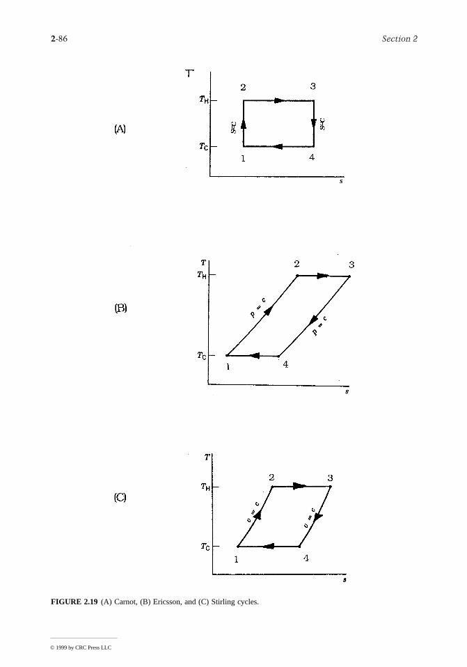
2-86 Section 2
FIGURE 2.19
(A) Carnot, (B) Ericsson, and (C) Stirling cycles.
s
© 1999 by CRC Press LLC
Engineering Thermodynamics 2-87
e costtifyingepartureaturalurther
ted toaction,
al with, butust be
ferent.
for the
goodnt suchrsibilityoducedtructionheatingr can betruction
ents ofures. In
cord-:
fer and, or to a
fer with
ith thetream-
etween
ndaryllowing
rbinesn to the
2.7 Guidelines for Improving Thermodynamic Effectiveness
Thermal design frequently aims at the most effective system from the cost viewpoint. Still, in thoptimization process, particularly of complex energy systems, it is often expedient to begin by idena design that is nearly optimal thermodynamically; such a design can then be used as a point of dfor cost optimization. Presented in this section are guidelines for improving the use of fuels (ngas, oil, and coal) by reducing sources of thermodynamic inefficiency in thermal systems. Fdiscussion is provided by Bejan et al. (1996).
To improve thermodynamic effectiveness it is necessary to deal directly with inefficiencies relaexergy destruction and exergy loss. The primary contributors to exergy destruction are chemical reheat transfer, mixing, and friction, including unrestrained expansions of gases and liquids. To dethem effectively, the principal sources of inefficiency not only should be understood qualitativelyalso determined quantitatively, at least approximately. Design changes to improve effectiveness mdone judiciously, however, for the cost associated with different sources of inefficiency can be difFor example, the unit cost of the electrical or mechanical power required to
provide for the exergydestroyed owing to a pressure drop is generally higher than the unit cost of the fuel required exergy destruction caused by combustion or heat transfer.
Since chemical reaction is a significant source of thermodynamic inefficiency, it is generally practice to minimize the use of combustion. In many applications the use of combustion equipmeas boilers is unavoidable, however. In these cases a significant reduction in the combustion irreveby conventional means simply cannot be expected, for the major part of the exergy destruction intrby combustion is an inevitable consequence of incorporating such equipment. Still, the exergy desin practical combustion systems can be reduced by minimizing the use of excess air and by prethe reactants. In most cases only a small part of the exergy destruction in a combustion chambeavoided by these means. Consequently, after considering such options for reducing the exergy desrelated to combustion, efforts to improve thermodynamic performance should focus on componthe overall system that are more amenable to betterment by cost-effective conventional measother words,
some exergy destructions and energy losses can be avoided
,
others cannot. Efforts shouldbe centered on those that can be avoided.
Nonidealities associated with heat transfer also typically contribute heavily to inefficiency. Ac
ingly, unnecessary or cost-ineffective heat transfer must be avoided. Additional guidelines follow
• The higher the temperature
T
at which a heat transfer occurs in cases where
T
>
T
0
, where
T
0
denotes the temperature of the environment (Section 2.5), the more valuable the heat transconsequently, the greater the need to avoid heat transfer to the ambient, to cooling water,refrigerated stream. Heat transfer across
T
0
should be avoided.
• The lower the temperature
T
at which a heat transfer occurs in cases where
T
<
T
0
, the morevaluable the heat transfer and, consequently, the greater the need to avoid direct heat transthe ambient or a heated stream.
• Since exergy destruction associated with heat transfer between streams varies inversely wtemperature level, the lower the temperature level, the greater the need to minimize the sto-stream temperature difference.
• Avoid the use of intermediate heat transfer fluids when exchanging energy by heat transfer btwo streams
Although irreversibilities related to friction, unrestrained expansion, and mixing are often secoin importance to those of combustion and heat transfer, they should not be overlooked, and the foguidelines apply:
• Relatively more attention should be paid to the design of the lower temperature stages of tuand compressors (the last stages of turbines and the first stages of compressors) tharemaining stages of these devices.
© 1999 by CRC Press LLC
2-88 Section 2
tions.
ective
rature,ring
ectively.
icystemg, and, and
o-dates (ifey of
ir
tute
ameter
• For turbines, compressors, and motors, consider the most thermodynamically efficient op
• Minimize the use of throttling; check whether power recovery expanders are a cost-effalternative for pressure reduction.
• Avoid processes using excessively large thermodynamic driving forces (differences in tempepressure, and chemical composition). In particular, minimize the mixing of streams diffesignificantly in temperature, pressure, or chemical composition.
• The greater the mass rate of flow, the greater the need to use the exergy of the stream eff
• The lower the temperature level, the greater the need to minimize friction.
Flowsheeting
or
process simulation
software can assist efforts aimed at improving thermodynameffectiveness by allowing engineers to readily model the behavior of an overall system, or scomponents, under specified conditions and do the required thermal analysis, sizing, costinoptimization. Many of the more widely used flowsheeting programs: ASPEN PLUS, PROCESSCHEMCAD are of the
sequential-modular
type. SPEEDUP is a popular program of the
equation-solver
type. Since process simulation is a rapidly evolving field, vendors should be contacted for up-tinformation concerning the features of flowsheeting software, including optimization capabilitieany). As background for further investigation of suitable software, see Biegler (1989) for a survthe capabilities of 15 software products.
References
Ahrendts, J. 1980. Reference states.
Energy Int. J.
5: 667–677.
ASHRAE Handbook 1993 Fundamentals
. 1993.
American Society of Heating, Refrigerating, and AConditioning Engineers, Atlanta.
ASME Steam Tables
, 6th ed. 1993. ASME Press, Fairfield, NJ.Bejan, A., Tsatsaronis, G., and Moran, M. 1996.
Thermal Design and Optimization
,
John
Wiley & Sons,New York
.
Biegler, L.T. 1989. Chemical process simulation.
Chem. Eng. Progr.
October: 50–61.Bird, R.B., Stewart, W.E., and Lightfoot, E.N. 1960.
Transport Phenomena
.
John
Wiley & Sons, NewYork
.
Bolz, R.E. and Tuve, G.L. (eds.). 1973. Handbook of Tables for Applied Engineering Science , 2nd ed.CRC Press, Boca Raton, FL.
Bornakke, C. and Sonntag, R.E. 1996.
Tables of Thermodynamic and Transport Properties
.
John
Wiley& Sons, New York
.
Cooper, H.W. and Goldfrank, J.C. 1967. B-W-R constants and new correlations.
Hydrocarbon Process-ing
.
46(12): 141–146
.
Gray, D.E. (ed.). 1972.
American Institute of Physics Handbook.
McGraw-Hill, New York.Haar, L. Gallagher, J.S., and Kell, G.S. 1984.
NBS/NRC Steam Tables
.
Hemisphere, New York
.Handbook of Chemistry and Physics
,
annual editions. CRC Press, Boca Raton, FL.
JANAF Thermochemical Tables
,
3rd ed. 1986. American Chemical Society and the American Instiof Physics for the National Bureau of Standards
.Jones, J.B. and Dugan, R.E. 1996. Engineering Thermodynamics. Prentice-Hall, Englewood Cliffs, NJ.Keenan, J.H., Keyes, F.G., Hill, P.G., and Moore, J.G. 1969 and 1978. Steam Tables. John Wiley &
Sons, New York (1969, English Units; 1978, SI Units).Keenan, J.H., Chao, J., and Kaye, J. 1980 and 1983. Gas Tables — International Version, 2nd ed. John
Wiley & Sons, New York (1980, English Units; 1983, SI Units).Knacke, O., Kubaschewski, O., and Hesselmann, K. 1991. Thermochemical Properties of Inorganic
Substances, 2nd ed. Springer-Verlag, Berlin.Kotas, T.J. 1995. The Exergy Method of Thermal Plant Analysis, Krieger, Melbourne, FL.Lee, B.I. and Kessler, M.G. 1975. A generalized thermodynamic correlation based on three-par
corresponding states. AIChE J. 21: 510–527.
© 1999 by CRC Press LLC
Engineering Thermodynamics
2
-89
l2.
y
sA.
r-
s
Liley, P.E. 1987. Thermodynamic properties of substances. In Marks’ Standard Handbook for MechanicaEngineers, E.A. Avallone and T. Baumeister, (eds.). 9th ed. McGraw-Hill, New York, Sec. 4.
Liley, P.E., Reid, R.C., and Buck, E. 1984. Physical and chemical data. In Perrys’ Chemical Engineers,Handbook, R.H. Perry and D.W. Green, (eds.). 6th ed. McGraw-Hill, New York, Sec. 3.
Moran, M.J. 1989. Availability Analysis — A Guide to Efficient Energy Use. ASME Press, New York.Moran, M.J. and Shapiro, H.N. 1995. Fundamentals of Engineering Thermodynamics, 3rd ed. John
Wiley & Sons, New York.Moran, M.J. and Shapiro, H.N. 1996. IT: Interactive Thermodynamics. Computer software to accompan
Fundamentals of Engineering Thermodynamics, 3rd ed. developed by Intellipro Inc., John Wiley& Sons, New York.
Obert, E.F. 1960. Concepts of Thermodynamics. McGraw-Hill, New York.Preston-Thomas, H. 1990. The International Temperature Scale of 1990 (ITS-90). Metrologia. 27: 3–10.Reid, R.C. and Sherwood, T.K. 1966. The Properties of Gases and Liquids, 2nd ed. McGraw-Hill, New
York.Reid, R.C., Prausnitz, J.M., and Poling, B.E. 1987. The Properties of Gases and Liquids, 4th ed. McGraw-
Hill, New York.Reynolds, W.C. 1979. Thermodynamic Properties in SI — Graphs, Tables and Computational Equation
for 40 Substances. Department of Mechanical Engineering, Stanford University, Palo Alto, CStephan, K. 1994. Tables. In Dubbel Handbook of Mechanical Engineering, W. Beitz and K.-H. Kuttner,
(eds.). Springer-Verlag, London, Sec. C11.Szargut, J., Morris, D.R., and Steward, F.R. 1988. Exergy Analysis of Thermal, Chemical and Metallu
gical Processes. Hemisphere, New York.Van Wylen, G.J., Sonntag, R.E., and Bornakke, C. 1994. Fundamentals of Classical Thermodynamic,
4th ed. John Wiley & Sons, New York.Wark, K. 1983. Thermodynamics, 4th ed. McGraw-Hill, New YorkZemansky, M.W. 1972. Thermodynamic symbols, definitions, and equations. In American Institute of
Physics Handbook, D.E. Gray, (ed.). McGraw-Hill, New York, Sec. 4b.
© 1999 by CRC Press LLC