more data with weka - department of computer science€¦ · more data mining with weka ... amount...

weka.waikato.ac.nz

Ian H. Witten

Department of Computer ScienceUniversity of Waikato

New Zealand

More Data Mining with Weka

Class 2 – Lesson 1

Discretizing numeric attributes

Lesson 2.1: Discretizing numeric attributes

Lesson 2.1 Discretization

Lesson 2.2 Supervised discretization

Lesson 2.3 Discretization in J48

Lesson 2.4 Document classification

Lesson 2.5 Evaluating 2‐class classification

Lesson 2.6 Multinomial Naïve Bayes

Class 1 Exploring Weka’s interfaces;working with big data

Class 2 Discretization and text classification

Class 3 Classification rules, association rules, and clustering

Class 4 Selecting attributes andcounting the cost

Class 5 Neural networks, learning curves, and performance optimization


Transforming numeric attributes to nominal

Equal‐width binning Equal‐frequency binning (“histogram equalization”) How many bins? Exploiting ordering information?


Equal‐width binning Open ionosphere.arff; use J48 91.5% (35 nodes)

– a01: values –1 (38) and +1 (313) [check with Edit…]– a03: scrunched up towards the top end– a04: normal distribution?

unsupervised>attribute>discretize: examine parameters 40 bins; all attributes; look at values 87.7% (81 nodes)

– a01:– a03:– a04: looks normal with some extra –1’s and +1’s

10 bins 86.6% (51 nodes) 5 bins 90.6% (46 nodes) 2 bins 90.9% (13 nodes)


Equal‐frequency binning ionosphere.arff; use J48 91.5% (35 nodes) equal‐frequency, 40 bins 87.2% (61 nodes)

– a01: only 2 bins– a03: flat with peak at +1 and small peaks at –1 and 0 (check Edit… window)– a04: flat with peaks at –1, 0, and +1

10 bins 89.5% (48 nodes) 5 bins 90.6% (28 nodes) 2 bins (look at attribute histograms!) 82.6% (47 nodes) How many bins?

(called “proportional k‐interval discretization”)∝


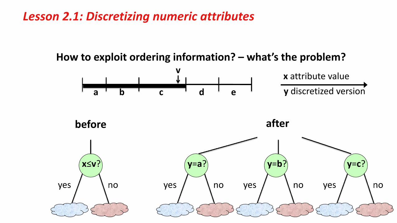
How to exploit ordering information? – what’s the problem?

after

x≤v?

yes no

y=a?

yes no

y=b?

yes no

y=c?

yes no

before

a b c d e

v x attribute valuey discretized version


How to exploit ordering information? – a solution Transform a discretized attribute with k values into k–1 binary attributes If the original attribute’s value is i for a particular instance, set the first i

binary attributes to true and the remainder to false

a b c d ez1z2z3z4

v x attributey discretized

binary


How to exploit ordering information? – a solution Transform a discretized attribute with k attributes into k–1 binary attributes If the original attribute’s value is i for a particular instance, set the first i


x ≤ va b c d e

z1 = true

z2 = true

z3 = true

z4 = false

v

z1z2z3z4

x attributey discretized

binary


How to exploit ordering information? – a solution Transform a discretized attribute with k attributes into k–1 binary attributes If the original attribute’s value is i for a particular instance, set the first i


z3?

yes no

x≤v?

yes no

before after


Equal‐width binning Equal‐frequency binning (“histogram equalization”) How many bins? Exploiting ordering information

Next … take the class into account (“supervised” discretization)

Course text Section 7.2 Discretizing numeric attributes

weka.waikato.ac.nz

Ian H. Witten


New Zealand



Supervised discretization and the FilteredClassifier

Lesson 2.2: Supervised discretization and the FilteredClassifier













What if all instances in a bin have one class, and all instances in the next higher bin have another class except for the first, which has the original class?

Take the class values into account – supervised discretization


c d

class 2class 1

x attributey discretized


Use the entropy heuristic (pioneered by C4.5 – J48 in Weka) e.g. temperature attribute of weather.numeric.arff dataset

Choose split point with smallest entropy (largest information gain) Repeat recursively until some stopping criterion is met


4 yes, 1 no 5 yes, 4 noentropy = 0.934 bits

amount of information required to specify the individual values of yes and no given the split


Supervised discretization: information‐gain‐based ionosphere.arff; use J48 91.5% (35 nodes) supervised>attribute>discretize: examine parameters apply filter: attributes range from 1–6 bins Use J48? – but there’s a problem with cross‐validation!

– test set has been used to help set the discretization boundaries – cheating!!!

(undo filtering) meta>FilteredClassifier: examine “More” info set up filter and J48 classifier; run: 91.2% (27 nodes) configure filter to set makeBinary 92.6% (17 nodes) cheat by pre‐discretizing using makeBinary 94.0% (17 nodes)


Supervised discretization– take class into account when making discretization boundaries

For test set, must use discretization determined by training set How can you do this when cross‐validating? FilteredClassifier: designed for exactly this situation Useful with other supervised filters too

Course text Section 7.2 Discretizing numeric attributes Section 11.3 Filtering algorithms, subsection “Supervised filters”

weka.waikato.ac.nz

Ian H. Witten


New Zealand



Discretization in J48

Lesson 2.3: Discretization in J48













Select attribute for root node– Create branch for each possible attribute value

Split instances into subsets– One for each branch extending from the node

Repeat recursively for each branch– using only instances that reach the branch

How does J48 deal with numeric attributes?Top‐down recursive divide‐and‐conquer (review)

Information gain Amount of information gained by knowing the value of the attribute (Entropy of distribution before the split) – (entropy of distribution after it)


Q: Which is the best attribute to split on?A (J48): The one with the greatest “information gain”

nnn ppppppppp log...loglog),...,,entropy( 221121

0.247 bits


Split‐point is a number … and there are infinitely many numbers! Split mid‐way between adjacent values in the training set n–1 possibilities (n is training set size); try them all!

Information gain for the temperature attribute

information gain = 0.001 bits

4 yes, 1 no 5 yes, 4 noentropy after the split = 0.939 bits

9 yes, 5 noentropy before the split = 0.940 bits


Further down the tree, split on humidity

humidity separates no’s from yes’ssplit halfway between {70,70} and {85}, i.e. 75 (!)

Outlook Temp Humidity Wind Play

Sunny 85 85 False No

Sunny 80 90 True No

Sunny 72 95 False No

Sunny 69 70 False Yes

Sunny 75 70 True Yes


Discretization boundaries are determined in a more specific context But based on a small subset of the overall information

… particularly lower down the tree, near the leaves

For every internal node, the instances that reach it must be sorted separately for every numeric attribute

… and sorting has complexity O(n log n) … but repeated sorting can be avoided with a better data structure

Discretization when building a tree vs. in advance

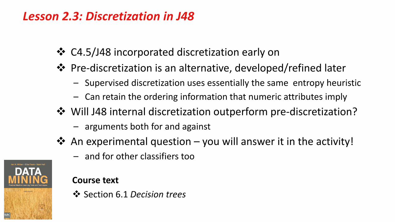
C4.5/J48 incorporated discretization early on Pre‐discretization is an alternative, developed/refined later

– Supervised discretization uses essentially the same entropy heuristic– Can retain the ordering information that numeric attributes imply

Will J48 internal discretization outperform pre‐discretization?– arguments both for and against

An experimental question – you will answer it in the activity!– and for other classifiers too

Course text Section 6.1 Decision trees


weka.waikato.ac.nz

Ian H. Witten


New Zealand



Document classification

Lesson 2.4: Document classification













Some training data

@relation 'training text’

@attribute text string@attribute type {yes, no}

@data'The price of crude oil has increased significantly', yes 'Demand of crude oil outstrips supply', yes 'Some people do not like the flavor of olive oil', no

Document text ClassificationThe price of crude oil has increased significantly yes Demand of crude oil outstrips supply yes Some people do not like the flavor of olive oil noThe food was very oily noCrude oil is in short supply yesUse a bit of cooking oil in the frying pan no


Load into Weka; note “string” attributes Apply StringToWordVector (unsupervised attribute filter) Creates 33 new attributes

– Crude, Demand, The, crude, has, in, increases, is, of, oil, …

Binary, numeric Use J48 (must set the class attribute) Evaluate on training set Visualize the tree


Supplied test set– set “Output predictions”

Problem evaluating classifier Apply StringToWordVector to test file?

– still get “Problem evaluating classifier”

Solution: FilteredClassifier– StringToWordVector creates attributes from training set– FilteredClassifier uses same attributes for test set

Result:– document 1 is “yes”; Documents 2, 3, 4 are “no”– (though document 3 should be “yes”)

Some test dataDocument text ClassificationOil platforms extract crude oil UnknownCanola oil is supposed to be healthy UnknownIraq has significant oil reserves UnknownThere are different types of cooking oil Unknown


Take a look at the dataset: ReutersCorn‐train.arff– it’s big: 1554 instances, 2 attributes

Apply StringToWordVector– it’s huge: 1554 instances, 2234 attributes (!)

Test set: ReutersCorn‐test.arff FilteredClassifier with StringToWordVector and J48

– (takes a while)

97% classification accuracy Look at model Look at confusion matrix:

– classification accuracy on 24 corn‐related documents: 15/24 = 62%– on remaining 580 documents: 573/580 = 99%

Is the overall classification accuracy really the right thing to optimize?


String attributes StringToWordVector filter: creates many attributes Check options for StringToWordVector J48 models for text data Overall classification accuracy

– is it really what we care about?– perhaps not

weka.waikato.ac.nz

Ian H. Witten


New Zealand



Evaluating 2‐class classification

Lesson 2.5: Evaluating 2‐class classification












===Confusion Matrix ===

a b <-- classified as

7 2 | a = yes

4 1 | b = no


Weather data; Naïve Bayes; 10‐fold cross‐validation

true positives

false positives

false negatives

true negatives

TP rate: TP / (TP + FN) = 7/9 = 0.78accuracy on class a

FP rate: FP / (FP + TN) = 4/5 = 0.801 – accuracy on class b

(negative instances that are incorrectly assigned to the positive class)

(taking “yes” as the positive class)


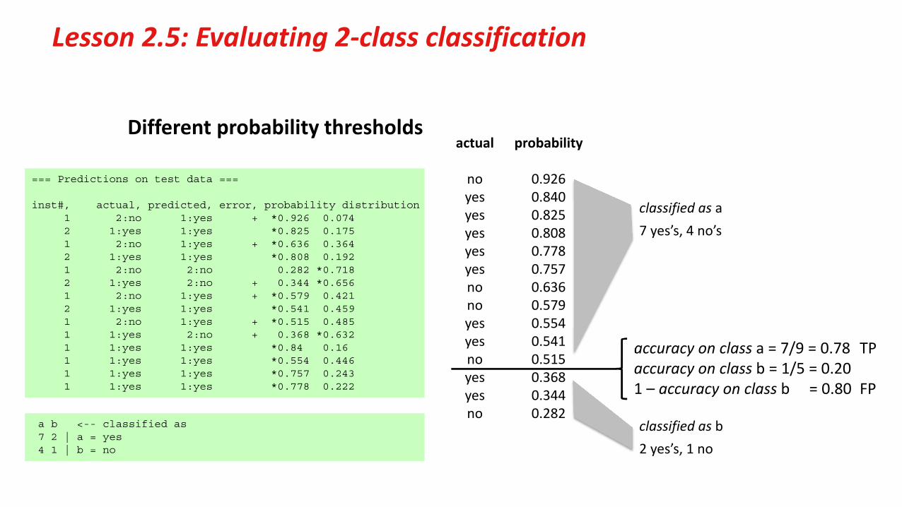
Different probability thresholdsactual probability

no 0.926yes 0.840yes 0.825yes 0.808yes 0.778yes 0.757no 0.636no 0.579yes 0.554yes 0.541no 0.515yes 0.368yes 0.344no 0.282

classified as a7 yes’s, 4 no’s

a b <-- classified as7 2 | a = yes4 1 | b = no

classified as b2 yes’s, 1 no

accuracy on class a = 7/9 = 0.78 TP accuracy on class b = 1/5 = 0.201 – accuracy on class b = 0.80 FP

=== Predictions on test data ===

inst#, actual, predicted, error, probability distribution1 2:no 1:yes + *0.926 0.0742 1:yes 1:yes *0.825 0.1751 2:no 1:yes + *0.636 0.3642 1:yes 1:yes *0.808 0.1921 2:no 2:no 0.282 *0.7182 1:yes 2:no + 0.344 *0.6561 2:no 1:yes + *0.579 0.4212 1:yes 1:yes *0.541 0.4591 2:no 1:yes + *0.515 0.4851 1:yes 2:no + 0.368 *0.6321 1:yes 1:yes *0.84 0.16 1 1:yes 1:yes *0.554 0.4461 1:yes 1:yes *0.757 0.2431 1:yes 1:yes *0.778 0.222

0


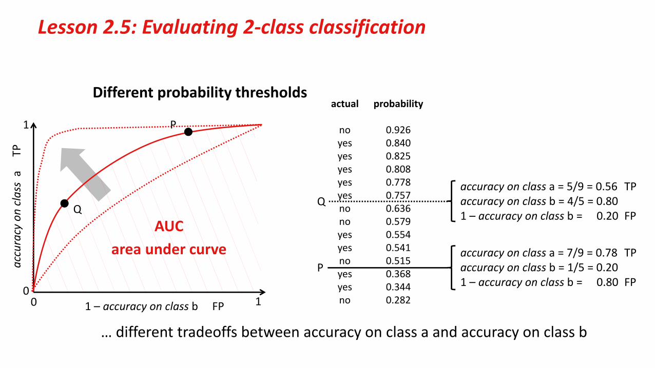
Different probability thresholdsactual probability


… different tradeoffs between accuracy on class a and accuracy on class b

0 1

1

P

Q

P

Q

accuracy on class a TP

1 – accuracy on class b FP

accuracy on class a = 5/9 = 0.56 TPaccuracy on class b = 4/5 = 0.801 – accuracy on class b = 0.20 FP

accuracy on class a = 7/9 = 0.78 TP accuracy on class b = 1/5 = 0.201 – accuracy on class b = 0.80 FP

AUCarea under curve


The “ROC” curve (Receiver Operating Characteristic: historical name)actual probability


FP rate TP rate

0/5 0/91/5 0/91/5 1/91/5 2/91/5 3/91/5 4/91/5 5/92/5 5/93/5 5/93/5 6/93/5 7/94/5 7/94/5 8/94/5 9/95/5 9/9

1 – accuracy on class b

accuracy on class a

accuracy on class a



Idealized “ROC” curves

accuracy on class a



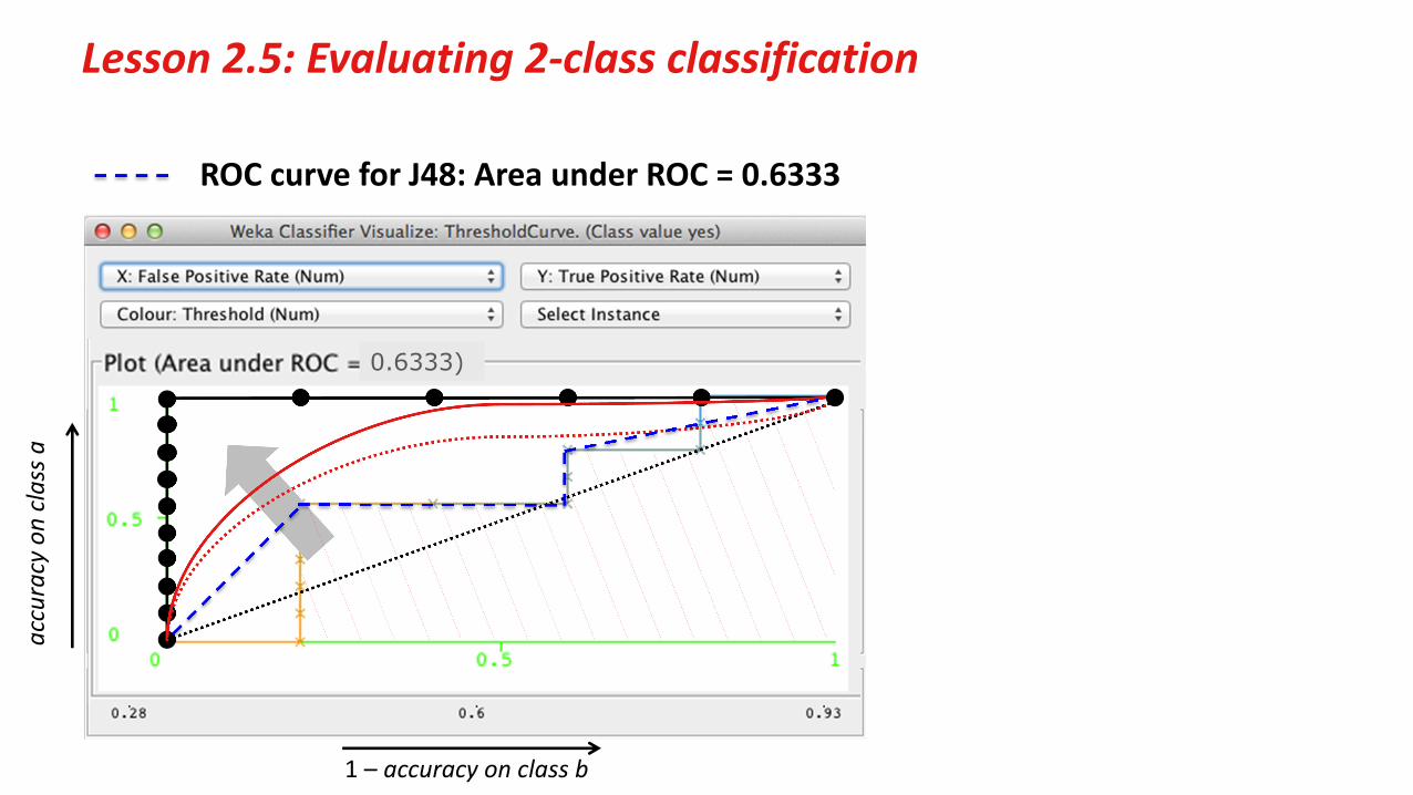
ROC curve for J48: Area under ROC = 0.6333

accuracy on class a


0.6333)

Course text Section 5.2 Counting the cost, subsection “ROC curves”


“Per‐class accuracy” threshold curves– points correspond to different tradeoffs between error types

ROC curves: TP rate (y axis) against FP rate (x axis)– go from lower left to upper right– good ones stretch up towards the top left corner– a diagonal line corresponds to a random decision

AUC (area under the [ROC] curve) – measures overall quality– probability that the classifier ranks a randomly chosen +ve test

instance above a randomly chosen –ve one

weka.waikato.ac.nz

Ian H. Witten


New Zealand



Multinomial Naïve Bayes

Lesson 2.6: Multinomial Naïve Bayes













Probability of event H given evidence E

Evidence splits into independent parts

Remember Naïve Bayes?

]Pr[]Pr[]|Pr[]|Pr[

EHHEEH

instanceclass

]|Pr[]...|Pr[]|Pr[]|Pr[ 21 HEHEHEHE n

Prior probability

Posterior probability

But– non‐appearance of a word counts just as strongly as appearance– does not account for multiple repetitions of a word– treats all words (common ones, unusual ones, …) the same

Document classification: Ei is appearance of word i


pi is probability of word i over all documents in class H

ni is number of times it appears in this document

N = n1+n2+…+nk is number of words in this document(the factorials “!” are a technicality to account for different word orderings)

Multinomial Naïve Bayes(for the curious)

k

i i

ni

npN

i

1 !!

]|Pr[]...|Pr[]|Pr[]|Pr[ 21 HEHEHEHE n


Training set: ReutersGrain‐train.arff; test set: ReutersGrain‐test.arff Classifier: FilteredClassifier with StringToWordVector J48 gets 96% classification accuracy

– 38/57 on corn‐related documents, 544/547 on others; ROC Area = 0.906

NaiveBayes: 80% classification accuracy– 46/57 on corn‐related documents, 439/547 on others; ROC Area = 0.885

NaiveBayesMultinomial: 91% classification accuracy– 52/57 on corn‐related documents, 496/547 on others; ROC Area = 0.973

Set outputWordCounts in StringToWordVectorNaiveBayesMultinomial: 91% classification accuracy– 54/57 on corn‐related documents, 496/547 on others; ROC Area = 0.962

Set lowerCaseTokens, useStoplist in StringToWordVectorNaiveBayesMultinomial: 93% classification accuracy– 56/57 on corn‐related documents, 504/547 on others; ROC Area = 0.978


Multinomial Naïve Bayes is designed for text– based on word appearance only, not non‐appearance– can account for multiple repetitions of a word– treats common words differently from unusual ones

It’s a lot faster than plain Naïve Bayes!– ignores words that do not appear in a document– internally, Weka uses a sparse representation of the data

The StringToWordVector filter has many interesting options– although they don’t necessarily give the results you’re looking for!– outputs results in “sparse data” format, which MNB takes advantage of

Course text Section 4.2 Statistical modeling, under “Naïve Bayes for document classification”

weka.waikato.ac.nz


New Zealand

creativecommons.org/licenses/by/3.0/

Creative Commons Attribution 3.0 Unported License
