1/46

Texture MappingMore Texture Mapping

2/46

Texture MappingPerturbing Normals

3/46

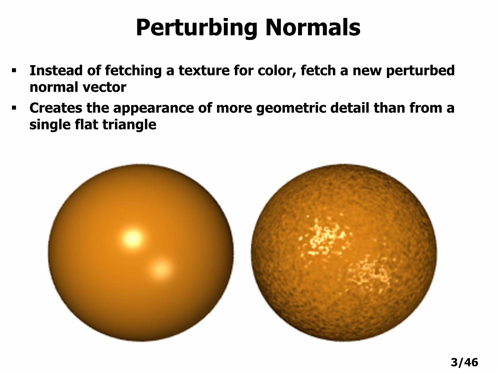
Perturbing Normals

Instead of fetching a texture for color, fetch a new perturbed normal vector

Creates the appearance of more geometric detail than from a single flat triangle

4/46

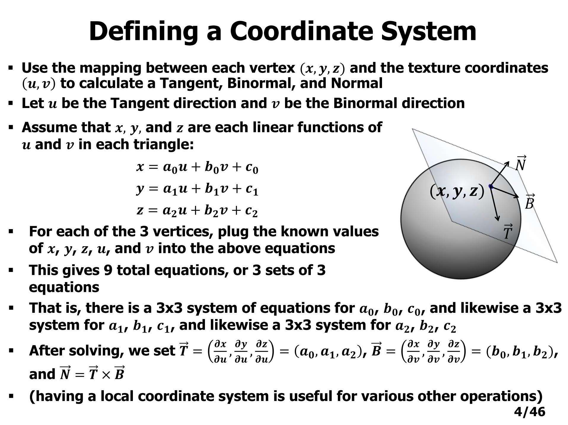
Use the mapping between each vertex (𝒙, 𝒚, 𝒛) and the texture coordinates 𝒖, 𝒗 to calculate a Tangent, Binormal, and Normal

Let 𝒖 be the Tangent direction and 𝒗 be the Binormal direction

Defining a Coordinate System

𝑇

𝐵

𝑁

(𝒙, 𝒚, 𝒛)

Assume that 𝒙, 𝒚, and 𝒛 are each linear functions of 𝒖 and 𝒗 in each triangle:

𝒙 = 𝒂𝟎𝒖 + 𝒃𝟎𝒗 + 𝒄𝟎

𝒚 = 𝒂𝟏𝒖 + 𝒃𝟏𝒗 + 𝒄𝟏

𝒛 = 𝒂𝟐𝒖 + 𝒃𝟐𝒗 + 𝒄𝟐

For each of the 3 vertices, plug the known values of 𝒙, 𝒚, 𝒛, 𝒖, and 𝒗 into the above equations

This gives 9 total equations, or 3 sets of 3 equations

That is, there is a 3x3 system of equations for 𝒂𝟎, 𝒃𝟎, 𝒄𝟎, and likewise a 3x3 system for 𝒂𝟏, 𝒃𝟏, 𝒄𝟏, and likewise a 3x3 system for 𝒂𝟐, 𝒃𝟐, 𝒄𝟐

After solving, we set 𝑻 =𝝏𝒙

𝝏𝒖,𝝏𝒚

𝝏𝒖,𝝏𝒛

𝝏𝒖= 𝒂𝟎, 𝒂𝟏, 𝒂𝟐 , 𝑩 =

𝝏𝒙

𝝏𝒗,𝝏𝒚

𝝏𝒗,𝝏𝒛

𝝏𝒗= (𝒃𝟎, 𝒃𝟏, 𝒃𝟐),

and 𝑵 = 𝑻 × 𝑩

(having a local coordinate system is useful for various other operations)

5/46

Perturbing the Normal

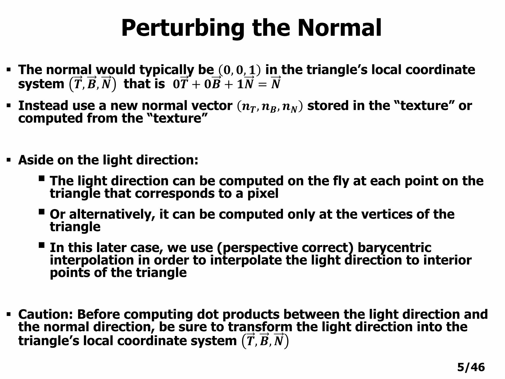
The normal would typically be 𝟎, 𝟎, 𝟏 in the triangle’s local coordinate system 𝑻,𝑩,𝑵 that is 𝟎𝑻 + 𝟎𝑩 + 𝟏𝑵 = 𝑵

Instead use a new normal vector 𝒏𝑻, 𝒏𝑩, 𝒏𝑵 stored in the “texture” or computed from the “texture”

Aside on the light direction:

The light direction can be computed on the fly at each point on the triangle that corresponds to a pixel

Or alternatively, it can be computed only at the vertices of the triangle

In this later case, we use (perspective correct) barycentricinterpolation in order to interpolate the light direction to interior points of the triangle

Caution: Before computing dot products between the light direction and the normal direction, be sure to transform the light direction into the triangle’s local coordinate system 𝑻,𝑩,𝑵

6/46

Bump Maps

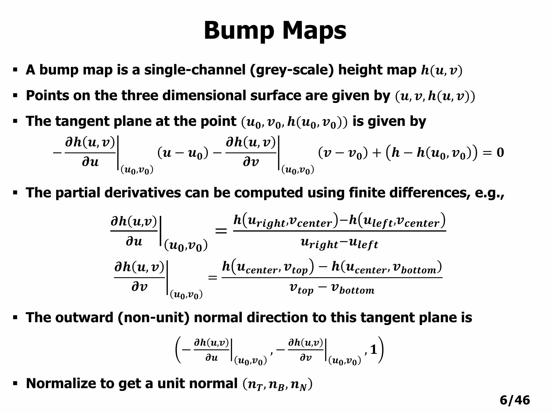
A bump map is a single-channel (grey-scale) height map 𝒉(𝒖, 𝒗)

Points on the three dimensional surface are given by (𝒖, 𝒗, 𝒉(𝒖, 𝒗))

The tangent plane at the point (𝒖𝟎, 𝒗𝟎, 𝒉(𝒖𝟎, 𝒗𝟎)) is given by

− ቤ𝝏𝒉 𝒖, 𝒗

𝝏𝒖𝒖𝟎,𝒗𝟎

𝒖 − 𝒖𝟎 − ቤ𝝏𝒉 𝒖, 𝒗

𝝏𝒗𝒖𝟎,𝒗𝟎

𝒗 − 𝒗𝟎 + 𝒉 − 𝒉 𝒖𝟎, 𝒗𝟎 = 𝟎

The partial derivatives can be computed using finite differences, e.g.,

ቚ𝝏𝒉 𝒖,𝒗

𝝏𝒖 𝒖𝟎,𝒗𝟎=

𝒉 𝒖𝒓𝒊𝒈𝒉𝒕,𝒗𝒄𝒆𝒏𝒕𝒆𝒓 −𝒉 𝒖𝒍𝒆𝒇𝒕,𝒗𝒄𝒆𝒏𝒕𝒆𝒓

𝒖𝒓𝒊𝒈𝒉𝒕−𝒖𝒍𝒆𝒇𝒕

ቤ𝝏𝒉 𝒖, 𝒗

𝝏𝒗𝒖𝟎,𝒗𝟎

=𝒉 𝒖𝒄𝒆𝒏𝒕𝒆𝒓, 𝒗𝒕𝒐𝒑 − 𝒉 𝒖𝒄𝒆𝒏𝒕𝒆𝒓, 𝒗𝒃𝒐𝒕𝒕𝒐𝒎

𝒗𝒕𝒐𝒑 − 𝒗𝒃𝒐𝒕𝒕𝒐𝒎

The outward (non-unit) normal direction to this tangent plane is

− ቚ𝝏𝒉 𝒖,𝒗

𝝏𝒖 𝒖𝟎,𝒗𝟎, − ቚ

𝝏𝒉 𝒖,𝒗

𝝏𝒗 𝒖𝟎,𝒗𝟎, 𝟏

Normalize to get a unit normal 𝒏𝑻, 𝒏𝑩, 𝒏𝑵

7/46

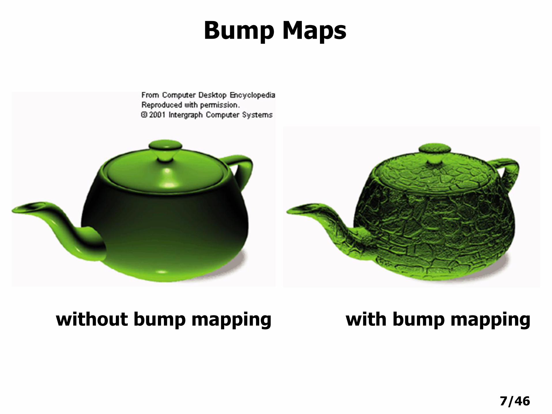
Bump Maps

without bump mapping with bump mapping

8/46

Normal Maps

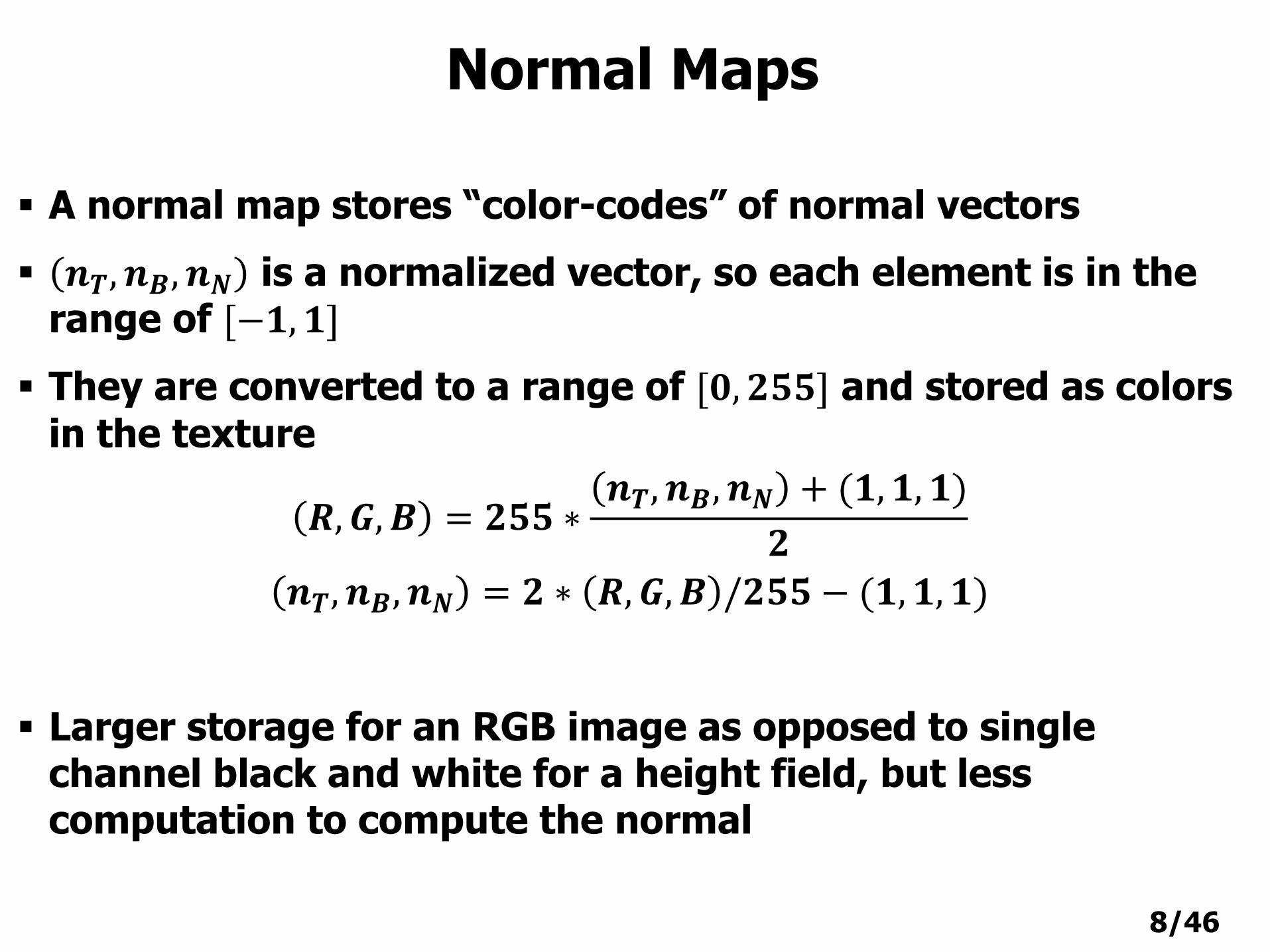
A normal map stores “color-codes” of normal vectors

𝒏𝑻, 𝒏𝑩, 𝒏𝑵 is a normalized vector, so each element is in the range of [−𝟏, 𝟏]

They are converted to a range of [𝟎, 𝟐𝟓𝟓] and stored as colors

in the texture

𝑹,𝑮,𝑩 = 𝟐𝟓𝟓 ∗𝒏𝑻, 𝒏𝑩, 𝒏𝑵 + (𝟏, 𝟏, 𝟏)

𝟐

𝒏𝑻, 𝒏𝑩, 𝒏𝑵 = 𝟐 ∗ 𝑹,𝑮, 𝑩 /𝟐𝟓𝟓 − (𝟏, 𝟏, 𝟏)

Larger storage for an RGB image as opposed to single channel black and white for a height field, but less computation to compute the normal

9/46

Normal Maps

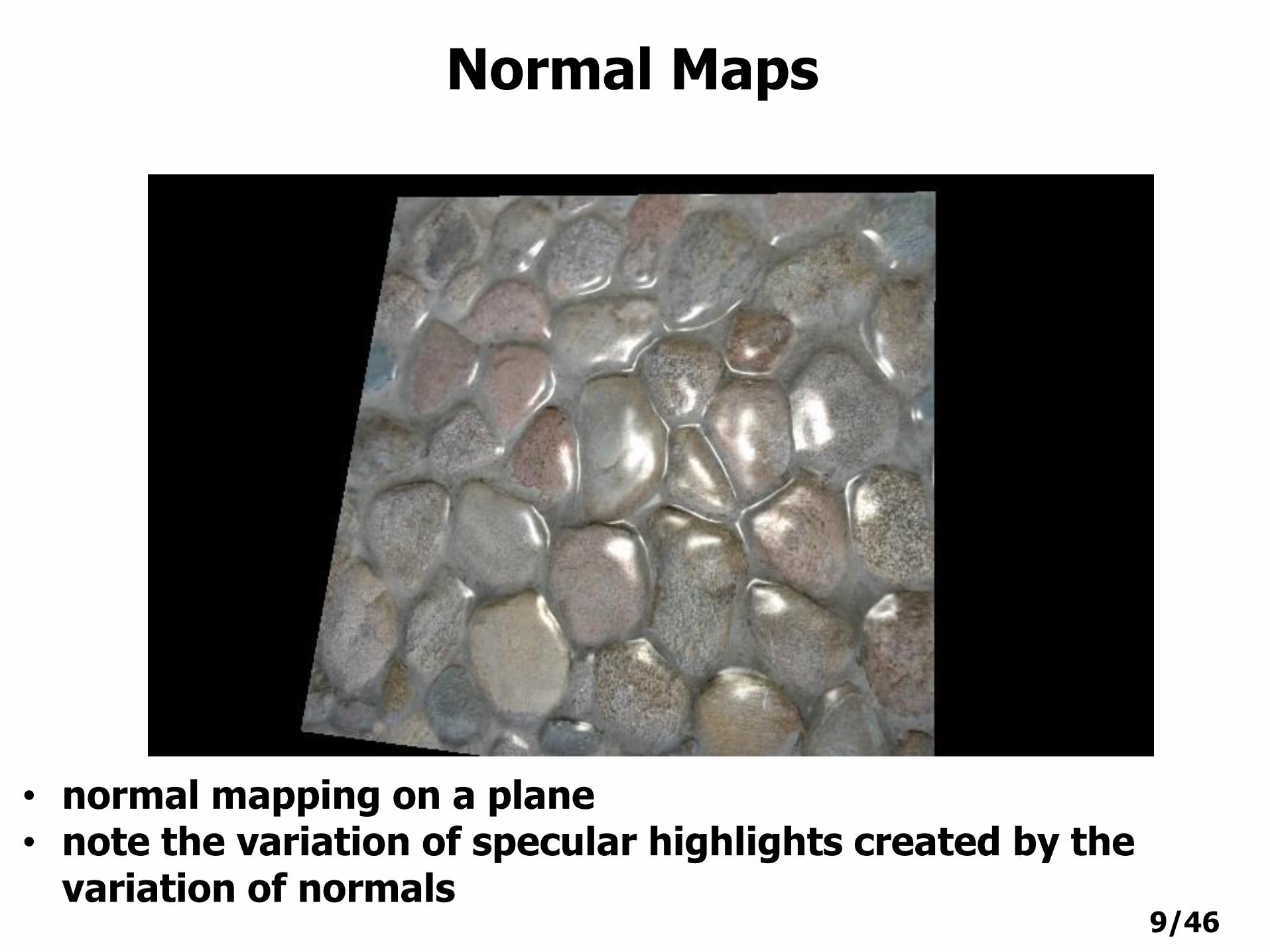
• normal mapping on a plane • note the variation of specular highlights created by the

variation of normals

10/46

Texture MappingPerturbing Geometry

11/46

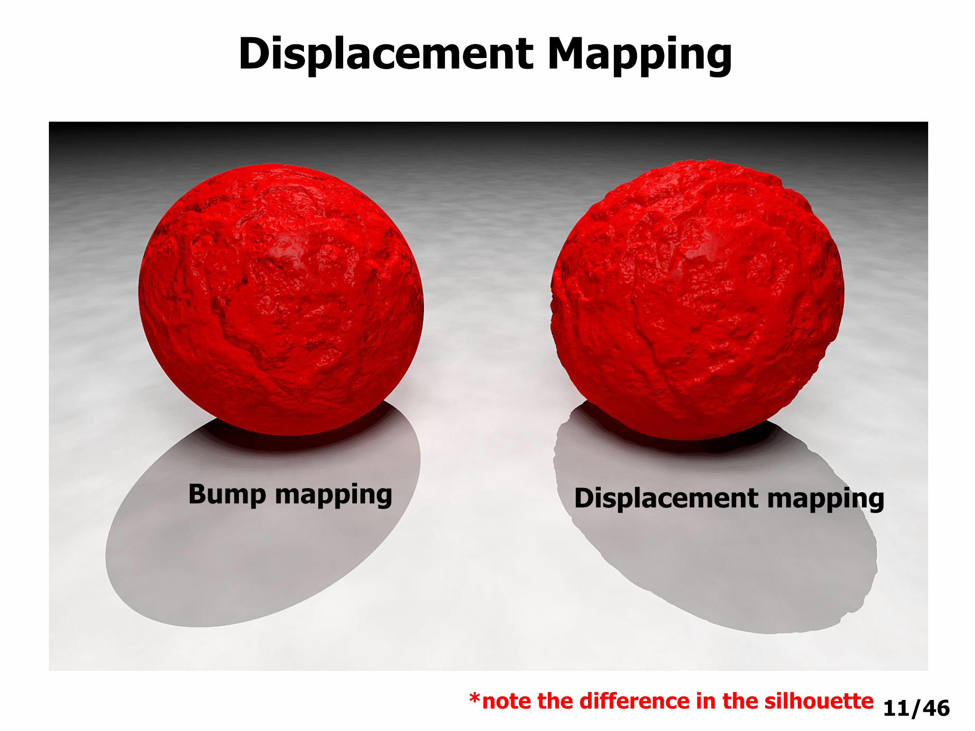
Displacement Mapping

Bump mapping Displacement mapping

*note the difference in the silhouette

12/46

Displacement Mapping

Perturb the surface geometry

Makes new (temporary) geometry on-the-fly at render time

The texture stores a height map 𝒉(𝒖, 𝒗). The texel values are used to perturb the vertices along the normal direction of the original geometry

Pros:

self-occlusion, self-shadowing

silhouettes and silhouette shadows appear correctly

Cons:

expensive

requires adaptive tessellation to ensure that the surface mesh is fine enough near perturbations

still need to bump/normal map for sub-triangle lighting variations

13/46

Displacement Mapping

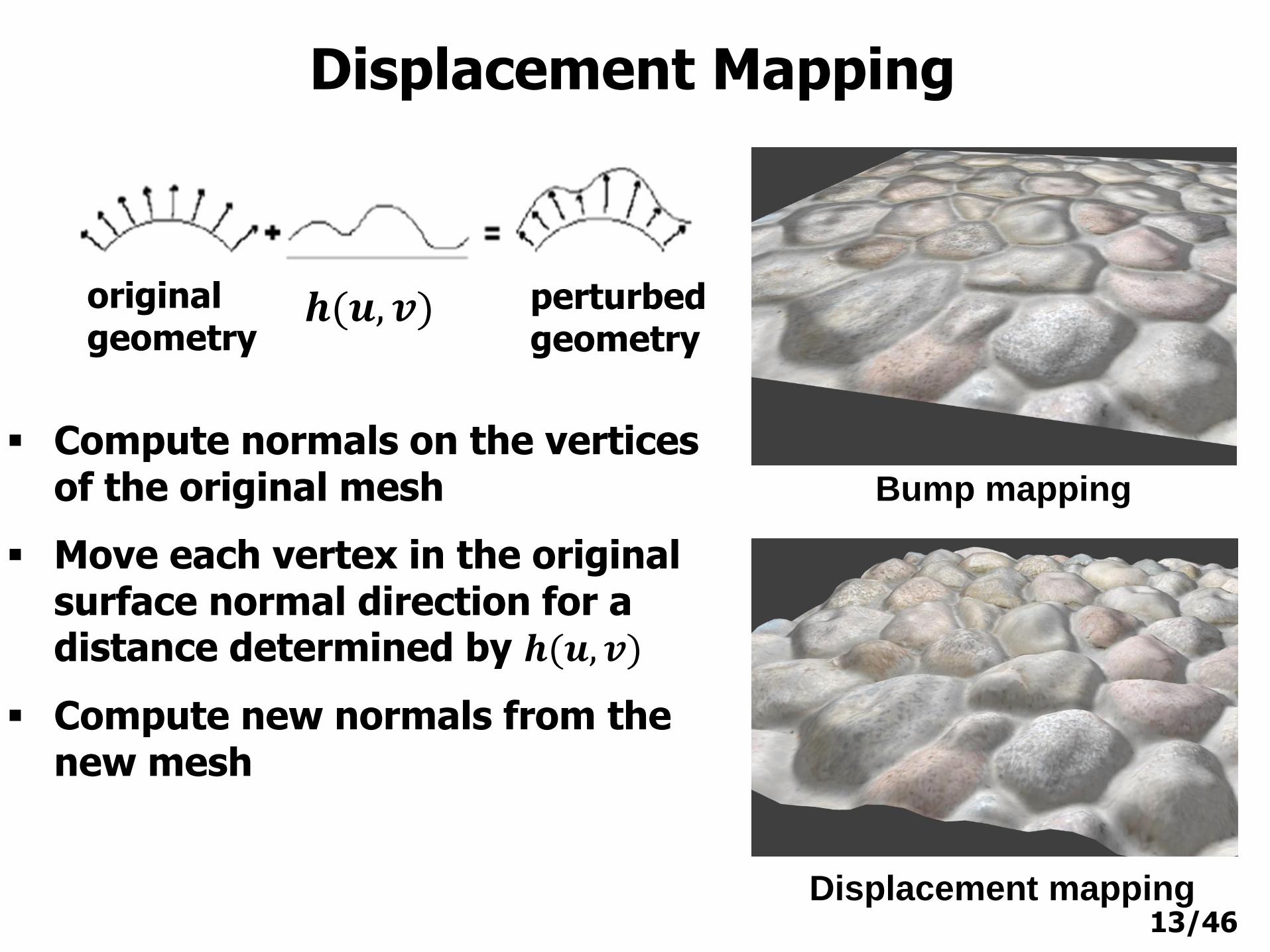
Bump mapping

Displacement mapping

𝒉(𝒖, 𝒗)originalgeometry

perturbedgeometry

Compute normals on the vertices of the original mesh

Move each vertex in the original surface normal direction for a distance determined by 𝒉(𝒖, 𝒗)

Compute new normals from the new mesh

14/46

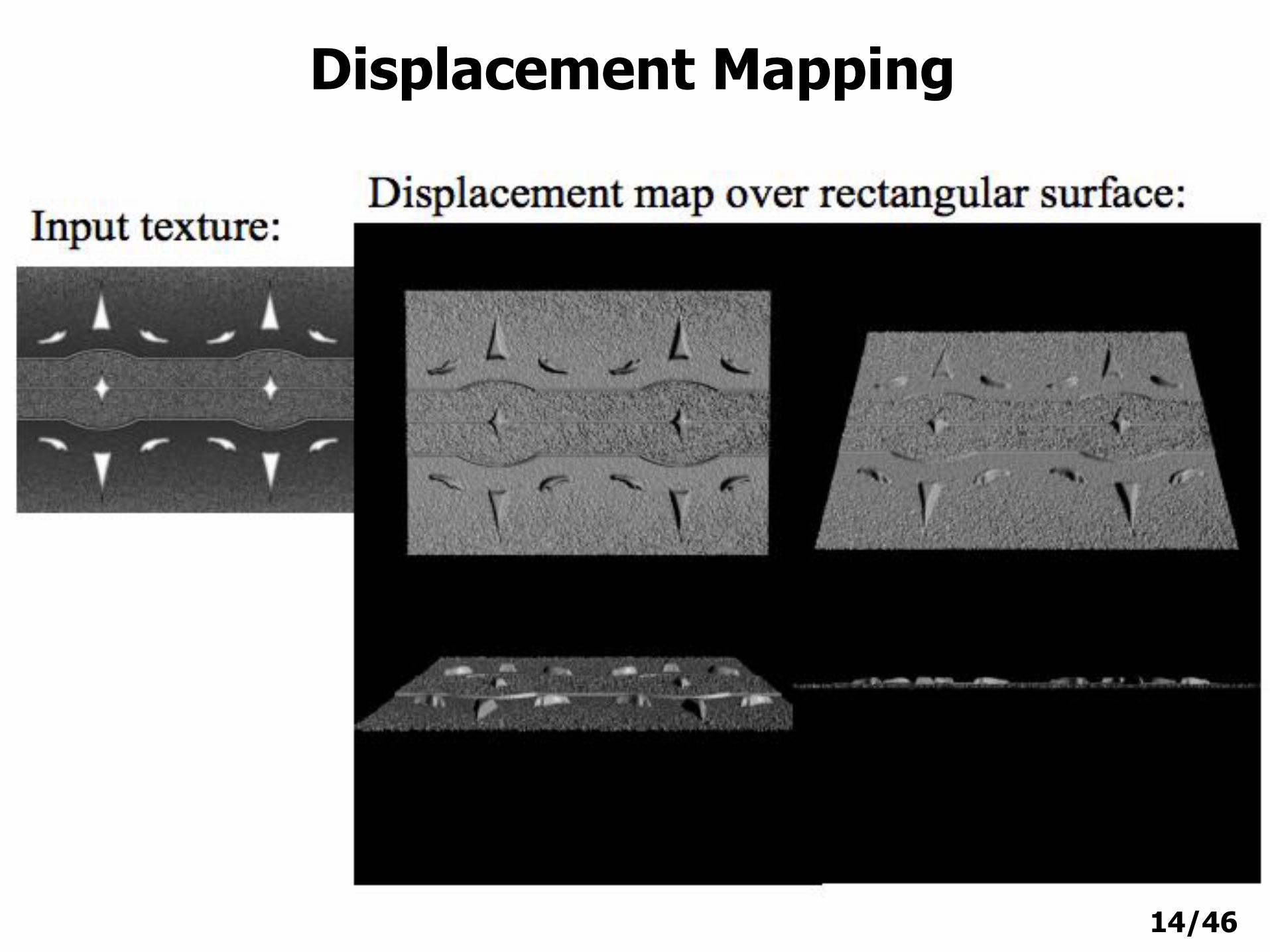
Displacement Mapping

15/46

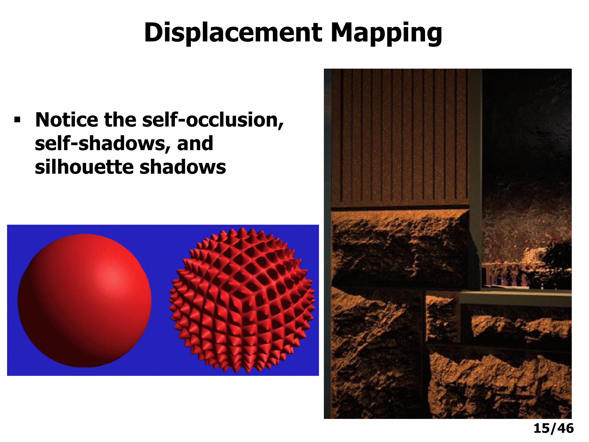
Displacement Mapping

Notice the self-occlusion, self-shadows, and silhouette shadows

16/46

Texture MappingEnvironment Mapping

17/46

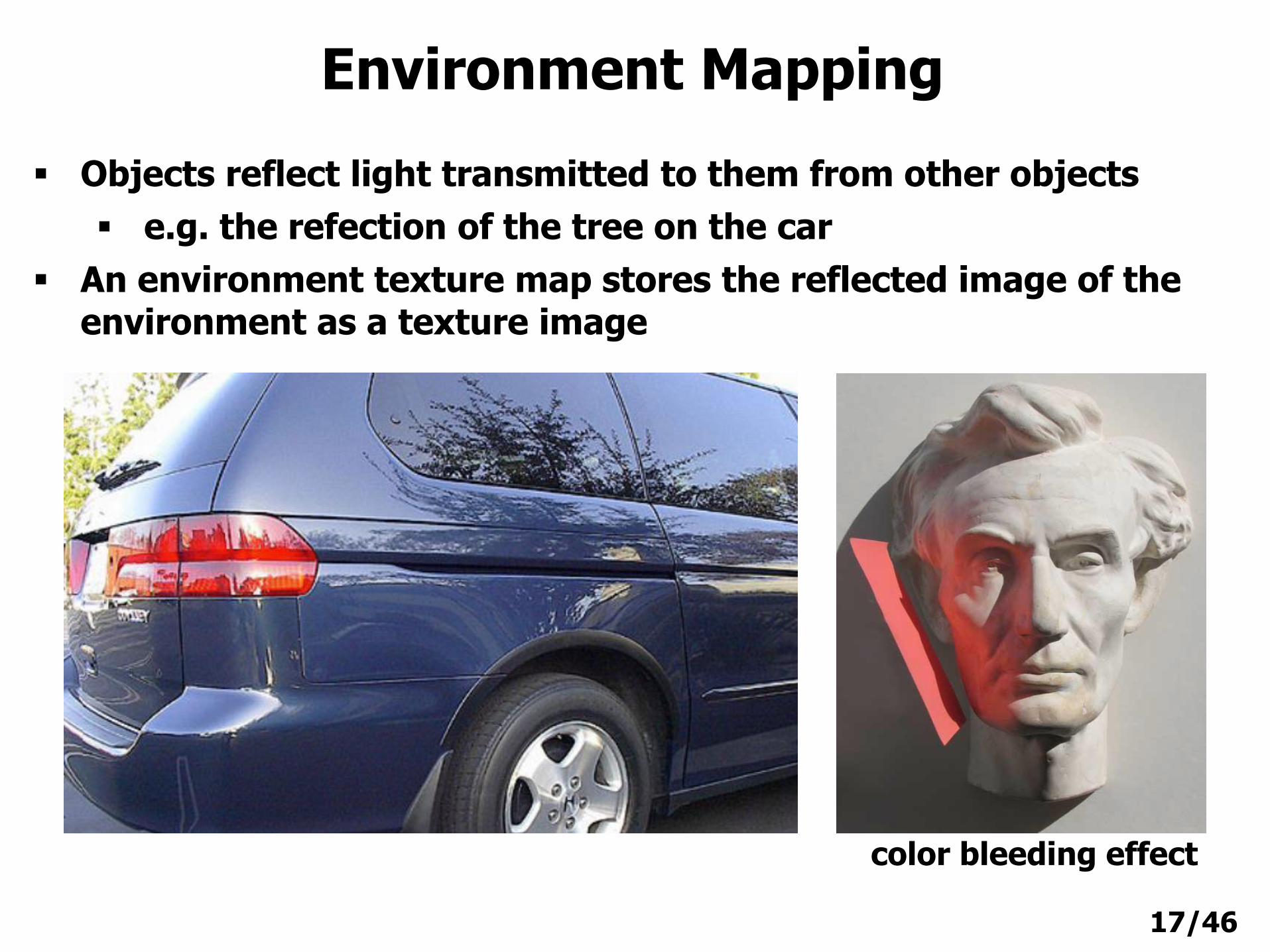
Environment Mapping

Objects reflect light transmitted to them from other objects

e.g. the refection of the tree on the car

An environment texture map stores the reflected image of the environment as a texture image

color bleeding effect

18/46

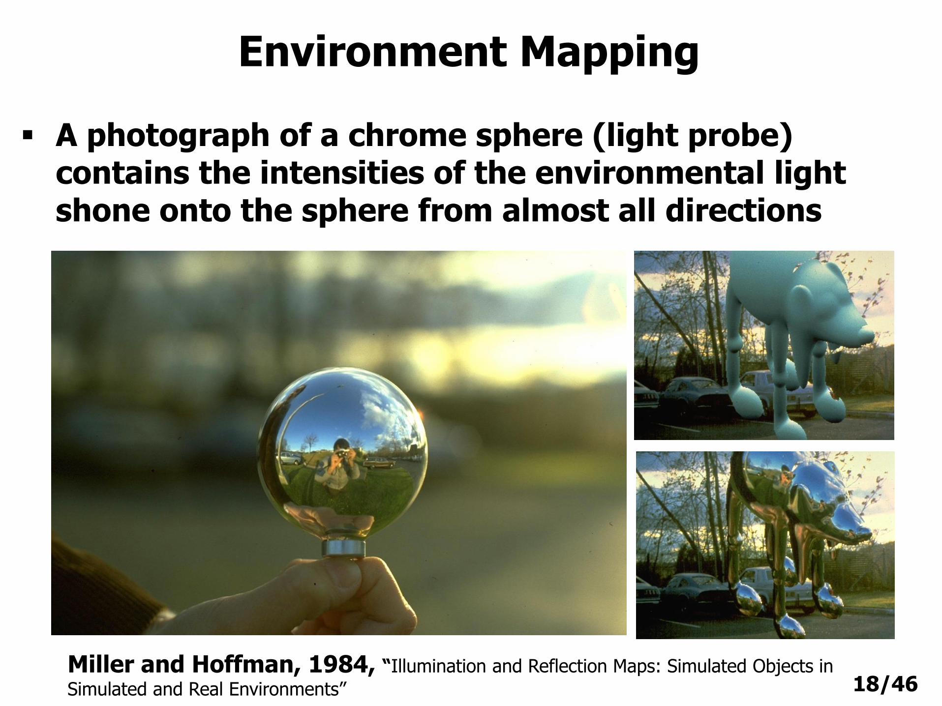
Environment Mapping

A photograph of a chrome sphere (light probe) contains the intensities of the environmental light shone onto the sphere from almost all directions

Miller and Hoffman, 1984, “Illumination and Reflection Maps: Simulated Objects in

Simulated and Real Environments”

19/46

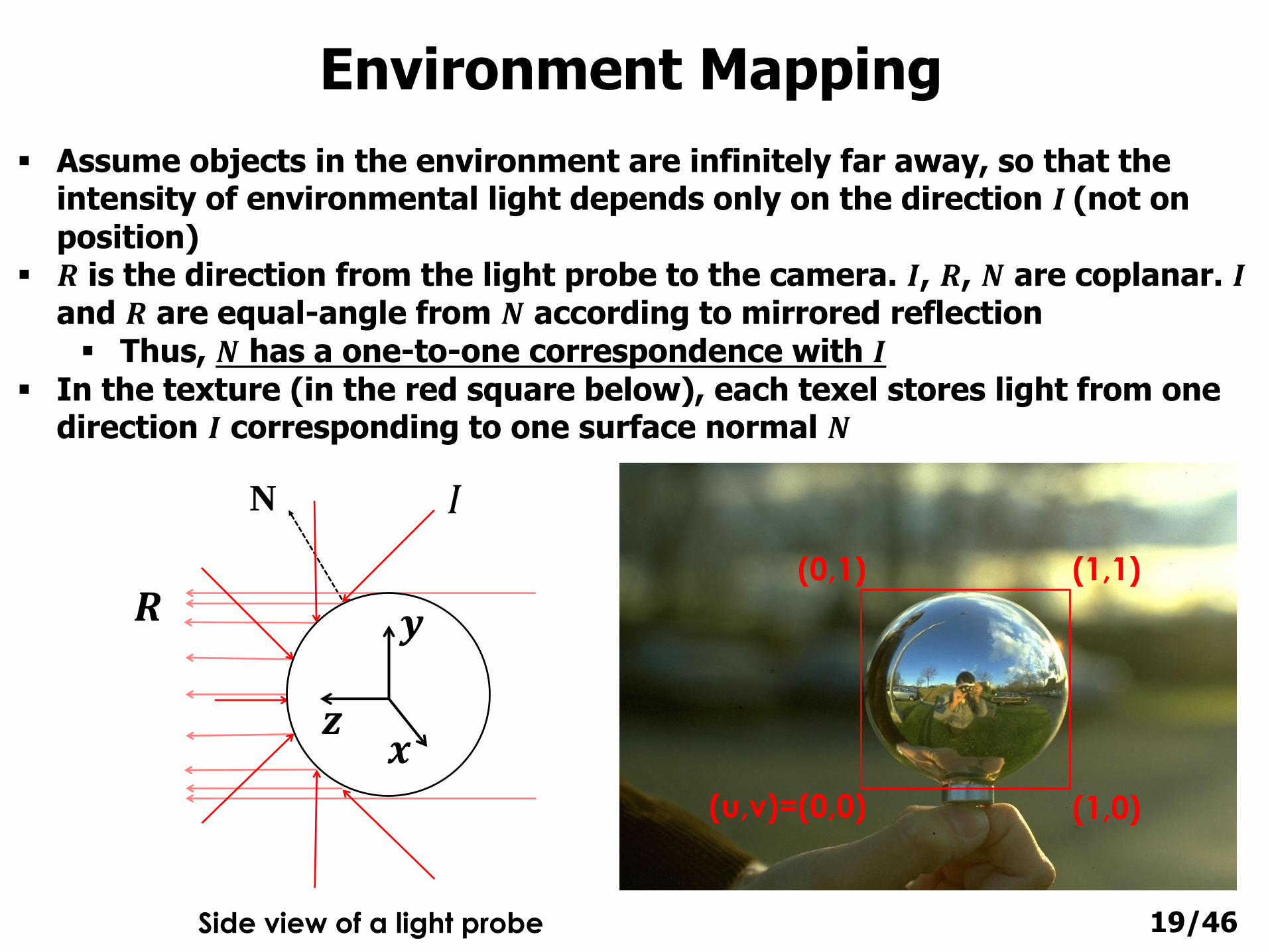
Assume objects in the environment are infinitely far away, so that the intensity of environmental light depends only on the direction 𝑰 (not on position)

𝑹 is the direction from the light probe to the camera. 𝑰, 𝑹, 𝑵 are coplanar. 𝑰and 𝑹 are equal-angle from 𝑵 according to mirrored reflection Thus, 𝑵 has a one-to-one correspondence with 𝑰

In the texture (in the red square below), each texel stores light from one direction 𝑰 corresponding to one surface normal 𝑵

Environment Mapping

Side view of a light probe

N 𝐼

𝑹 𝒚

𝒛𝒙

(u,v)=(0,0) (1,0)

(1,1)(0,1)

20/46

(u,v)=(0,0) (1,0)

(1,1)(0,1)

Environment Mapping

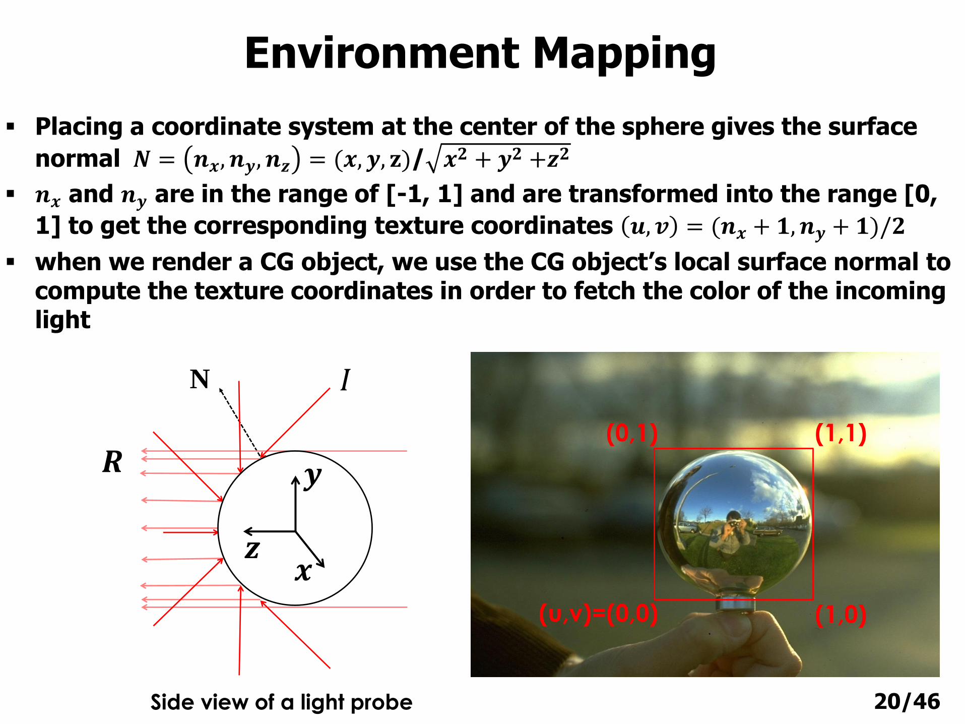
Placing a coordinate system at the center of the sphere gives the surface

normal 𝑵 = 𝒏𝒙, 𝒏𝒚, 𝒏𝒛 = (𝒙, 𝒚, 𝐳)/ 𝒙𝟐 + 𝒚𝟐 +𝒛𝟐

𝒏𝒙 and 𝒏𝒚 are in the range of [-1, 1] and are transformed into the range [0,

1] to get the corresponding texture coordinates 𝒖, 𝒗 = (𝒏𝒙 + 𝟏, 𝒏𝒚 + 𝟏)/𝟐

when we render a CG object, we use the CG object’s local surface normal to compute the texture coordinates in order to fetch the color of the incoming light

Side view of a light probe

N 𝐼

𝑹 𝒚

𝒛𝒙

21/46

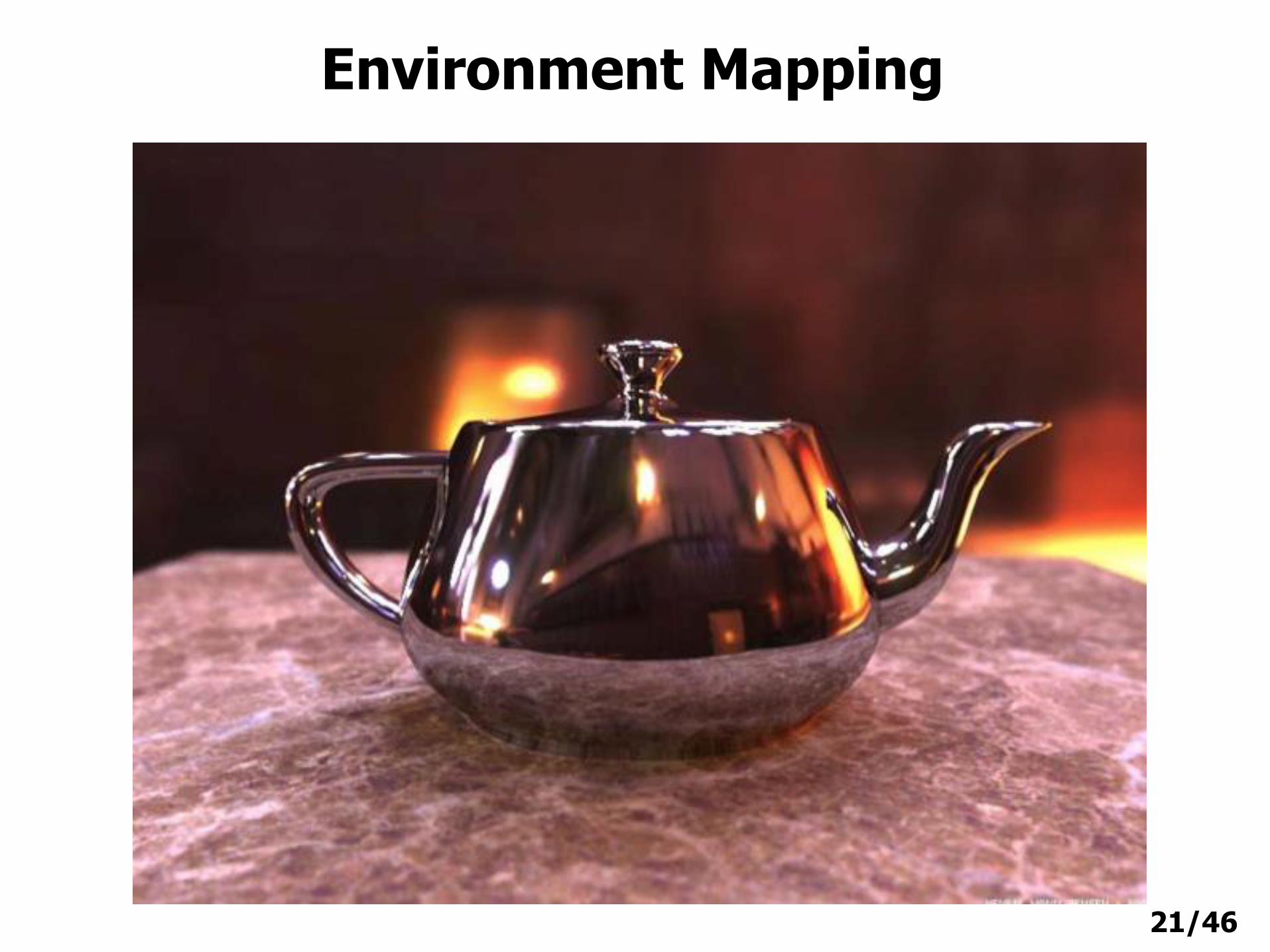
Environment Mapping

22/46

Texture MappingMaking Textures

23/46

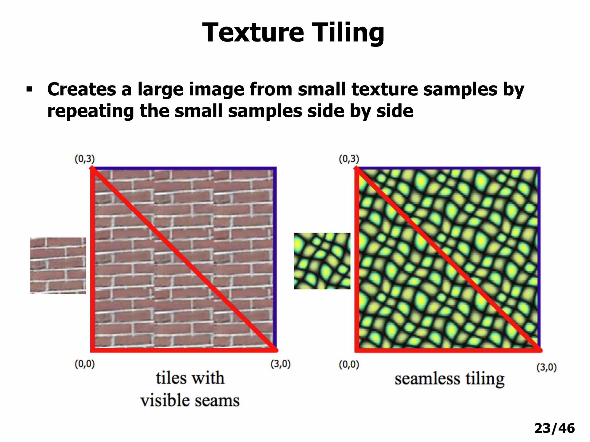
Texture Tiling

Creates a large image from small texture samples by repeating the small samples side by side

24/46

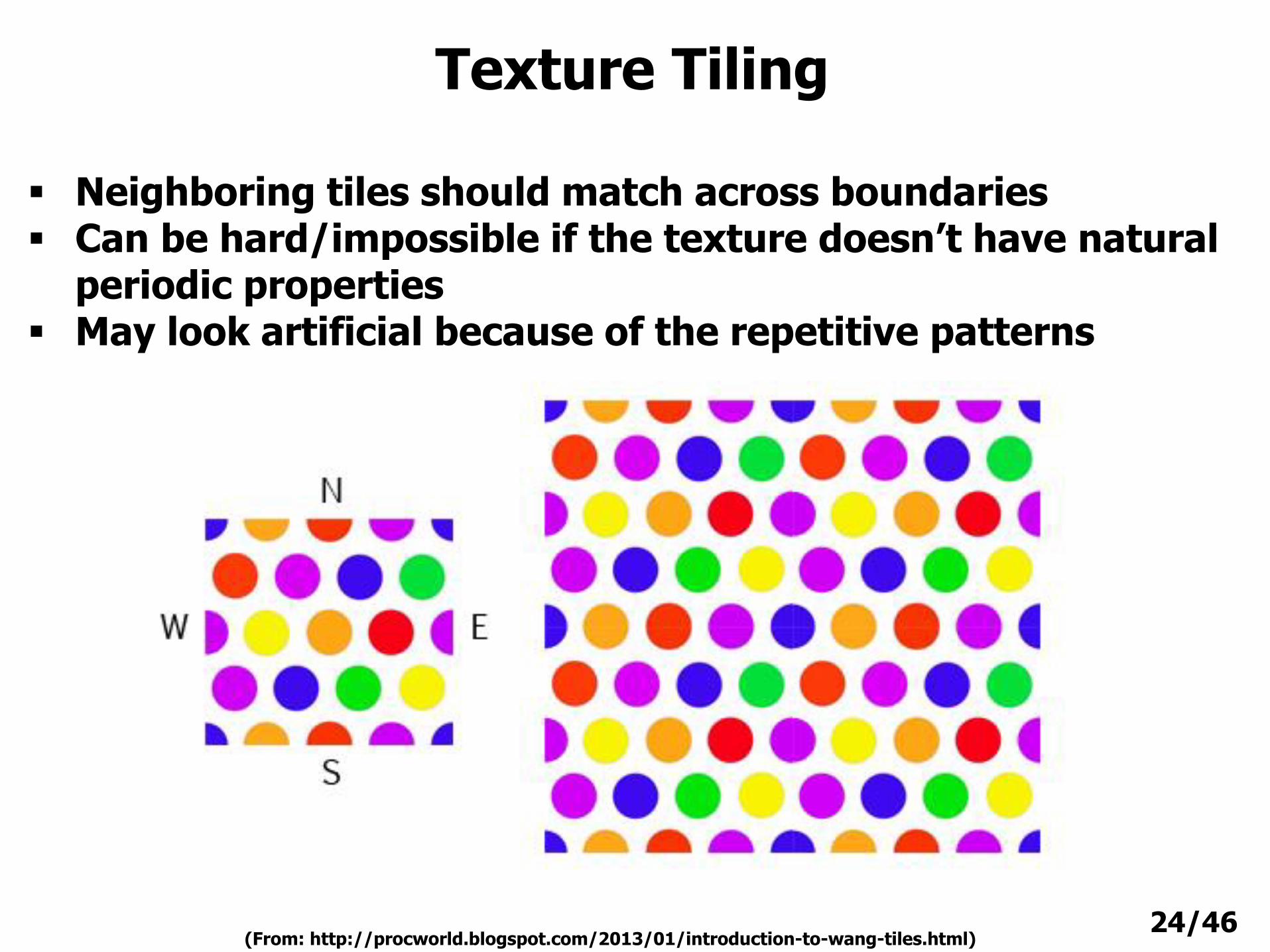
Texture Tiling

Neighboring tiles should match across boundaries Can be hard/impossible if the texture doesn’t have natural

periodic properties May look artificial because of the repetitive patterns

(From: http://procworld.blogspot.com/2013/01/introduction-to-wang-tiles.html)

25/46

Texture Synthesis

Create a large non-repetitive texture from a small sample by using its structural content

Algorithms for texture synthesis are typically either pixel based or patch based

Pixel-based algorithms - generate one pixel at a time

Patch-based algorithms - generate one block/patch at a time

26/46

Texture Synthesis: Pixel-based

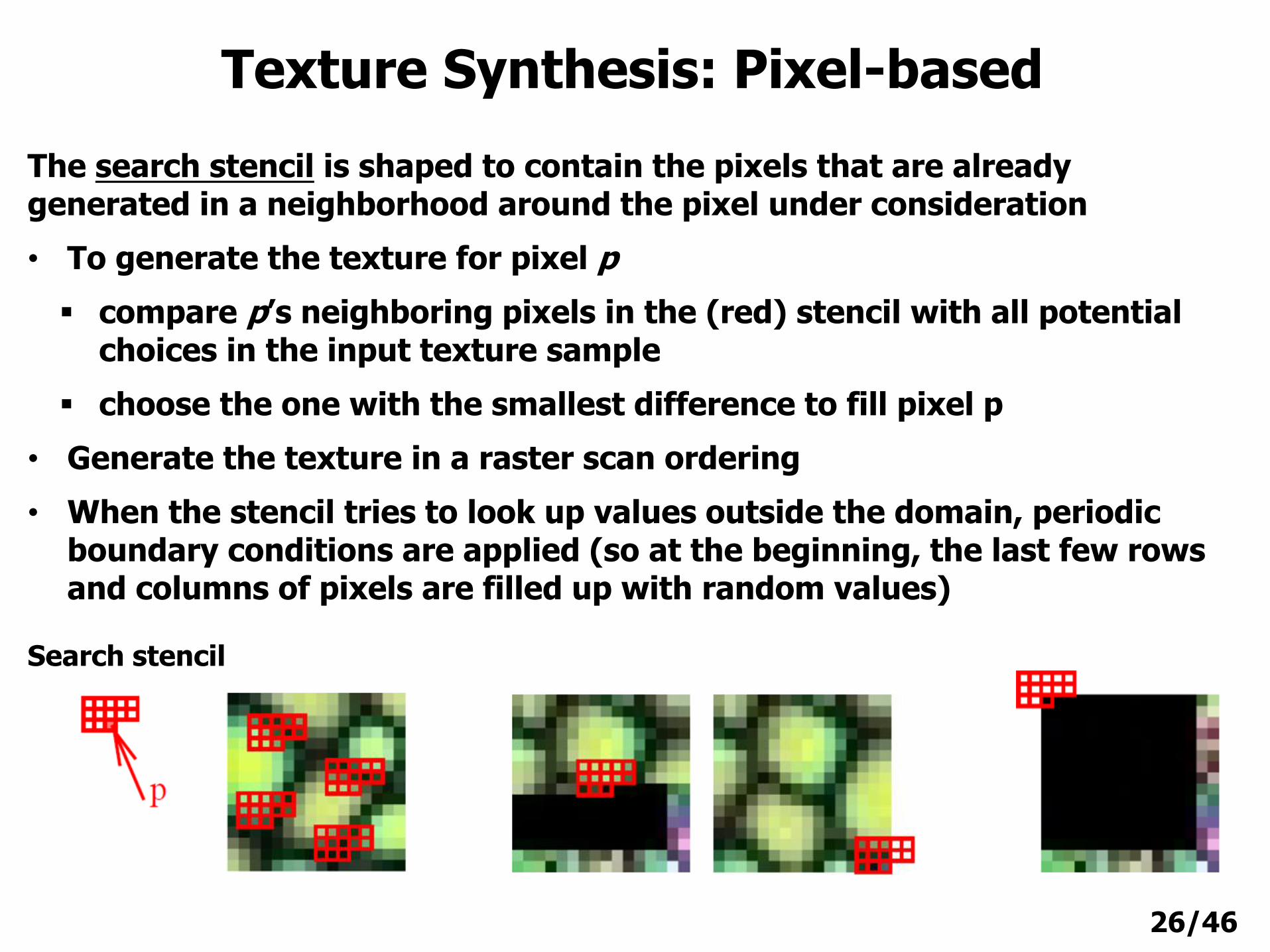
The search stencil is shaped to contain the pixels that are already generated in a neighborhood around the pixel under consideration

• To generate the texture for pixel p

compare p’s neighboring pixels in the (red) stencil with all potential choices in the input texture sample

choose the one with the smallest difference to fill pixel p

• Generate the texture in a raster scan ordering

• When the stencil tries to look up values outside the domain, periodic boundary conditions are applied (so at the beginning, the last few rows and columns of pixels are filled up with random values)

Search stencil

27/46

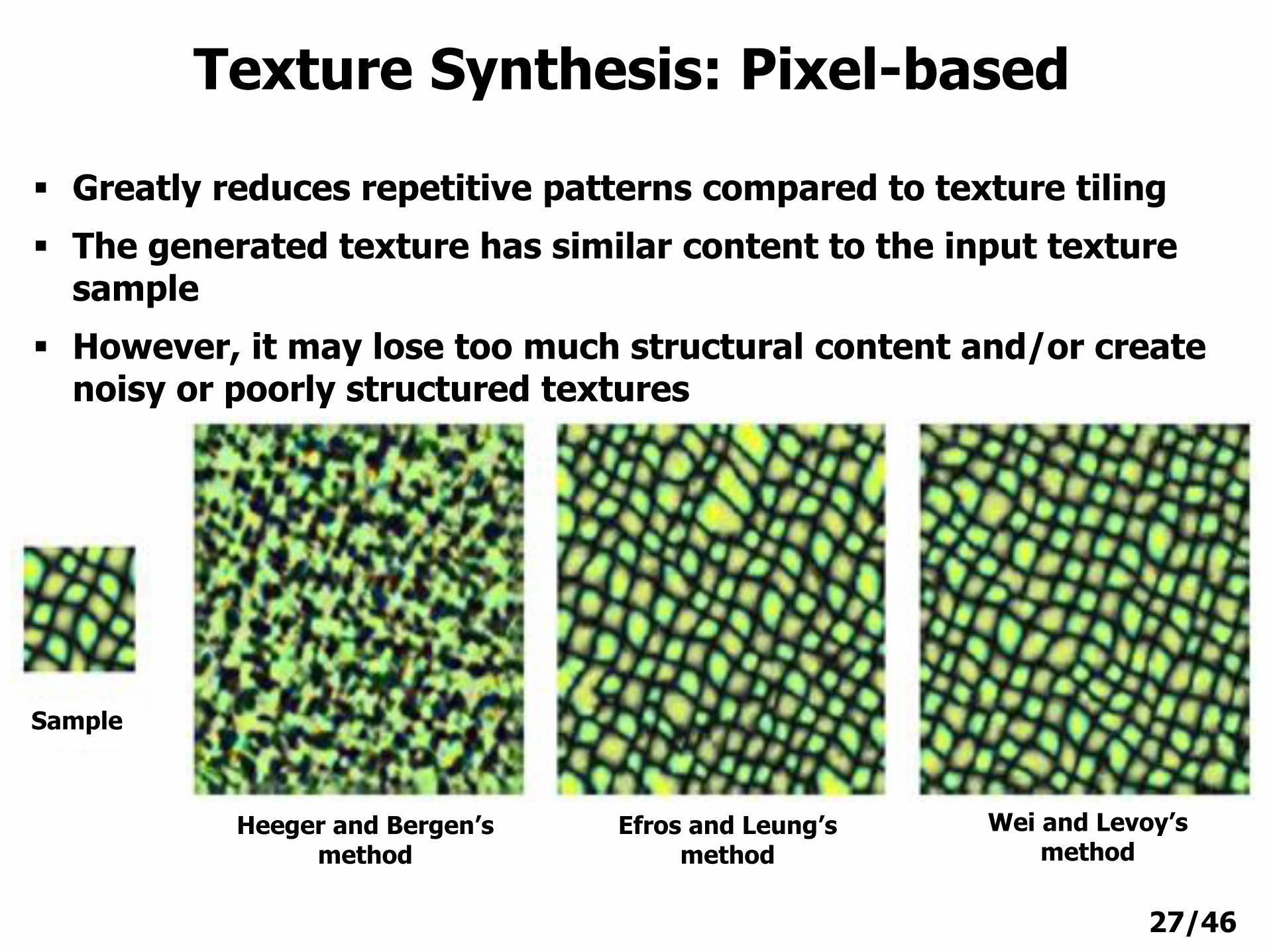
Texture Synthesis: Pixel-based

Greatly reduces repetitive patterns compared to texture tiling

The generated texture has similar content to the input texture sample

However, it may lose too much structural content and/or create noisy or poorly structured textures

Heeger and Bergen’s method

Efros and Leung’s method

Wei and Levoy’smethod

Sample

28/46

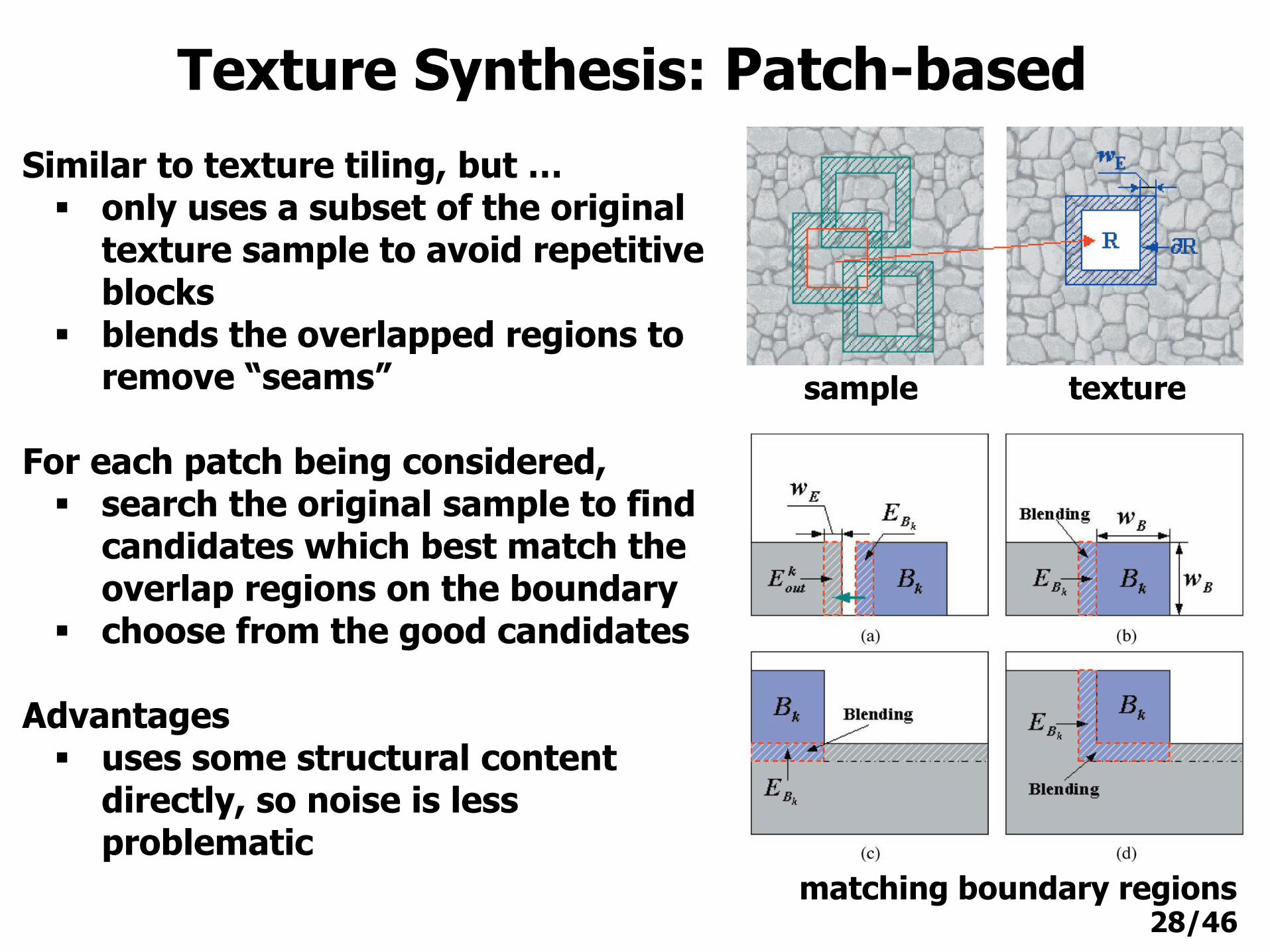
Texture Synthesis: Patch-based

Similar to texture tiling, but … only uses a subset of the original

texture sample to avoid repetitive blocks

blends the overlapped regions to remove “seams”

For each patch being considered, search the original sample to find

candidates which best match the overlap regions on the boundary

choose from the good candidates

Advantages uses some structural content

directly, so noise is less problematic

sample texture

matching boundary regions

29/46

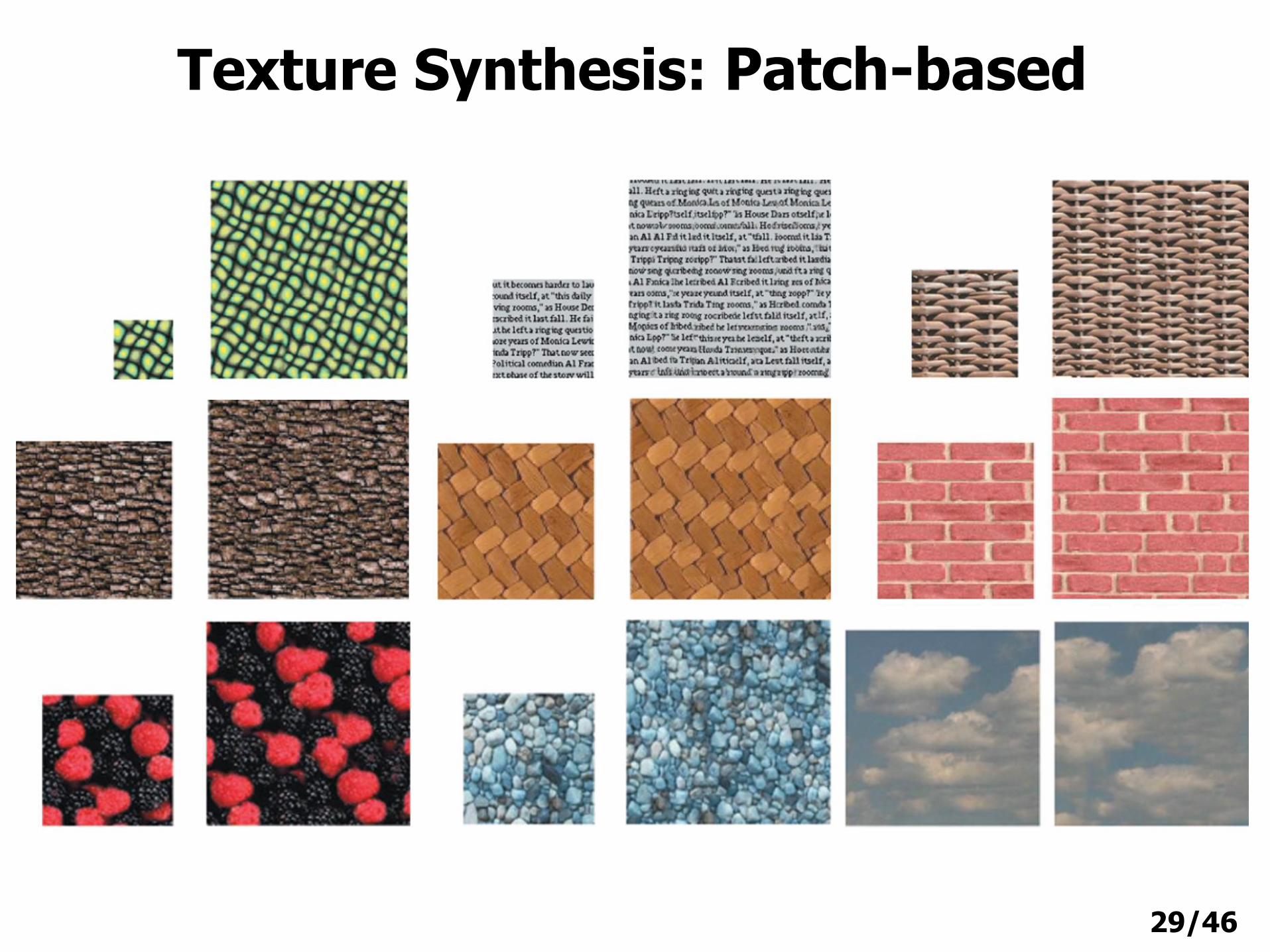
Texture Synthesis: Patch-based

30/46

Procedural Textures

Created/generated using a mathematical/computational algorithm

Good for generating natural elements

e.g. wood, marble, granite, stone, etc.

The natural look is achieved using noise or turbulence functions

These turbulence functions are used as a numerical representation of the “randomness” found in nature

31/46

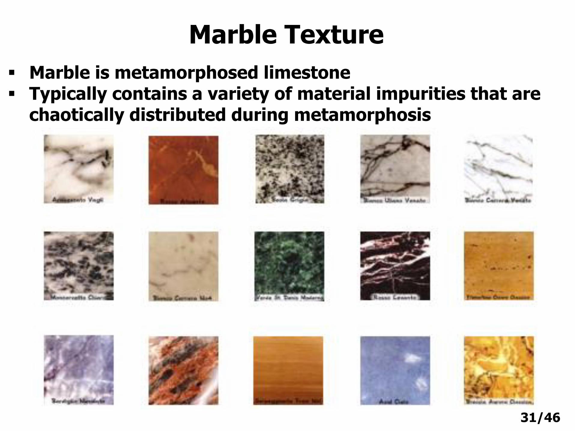
Marble Texture

Marble is metamorphosed limestone Typically contains a variety of material impurities that are

chaotically distributed during metamorphosis

32/46

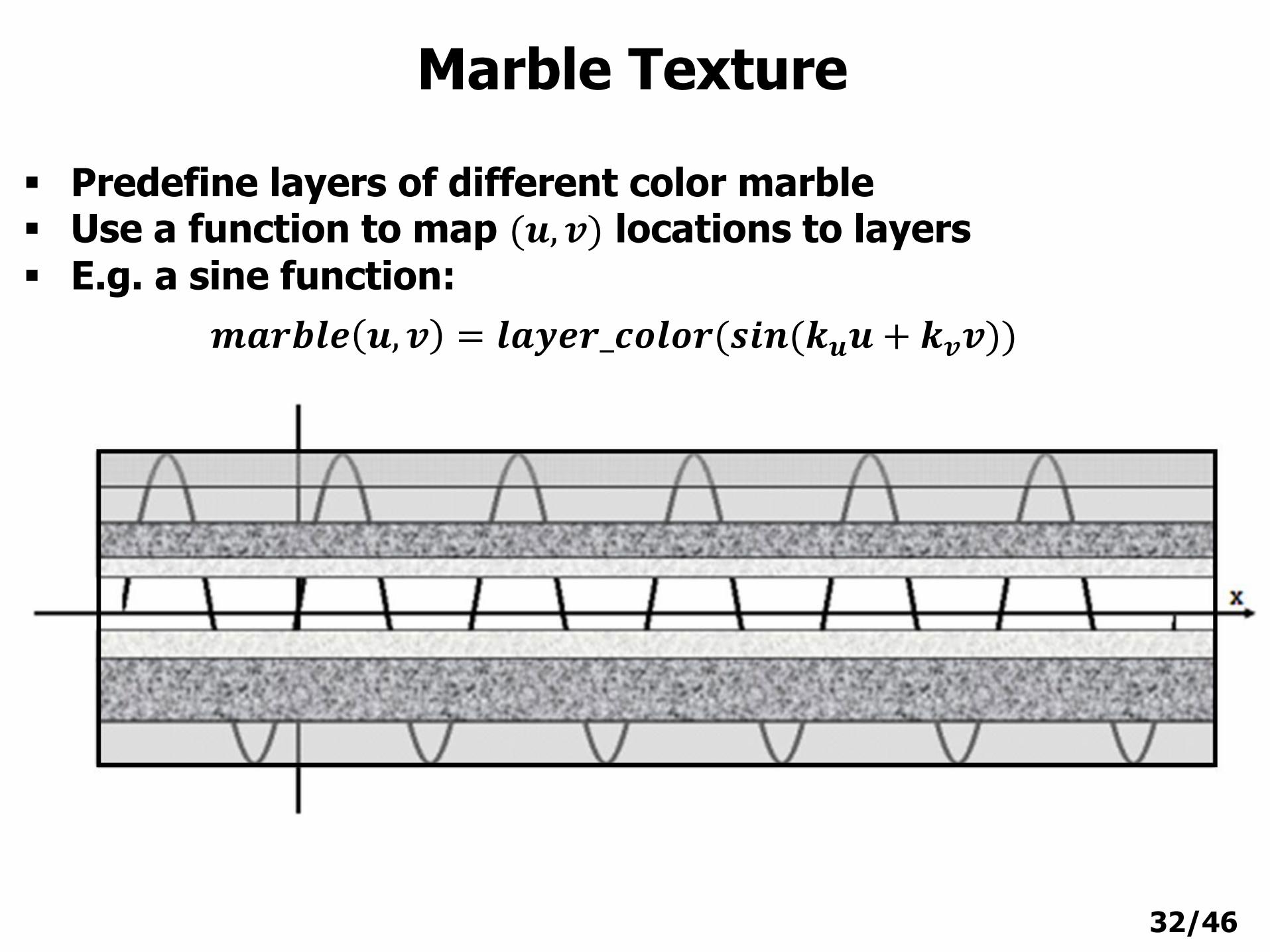
Predefine layers of different color marble Use a function to map (𝒖, 𝒗) locations to layers E.g. a sine function:

Marble Texture

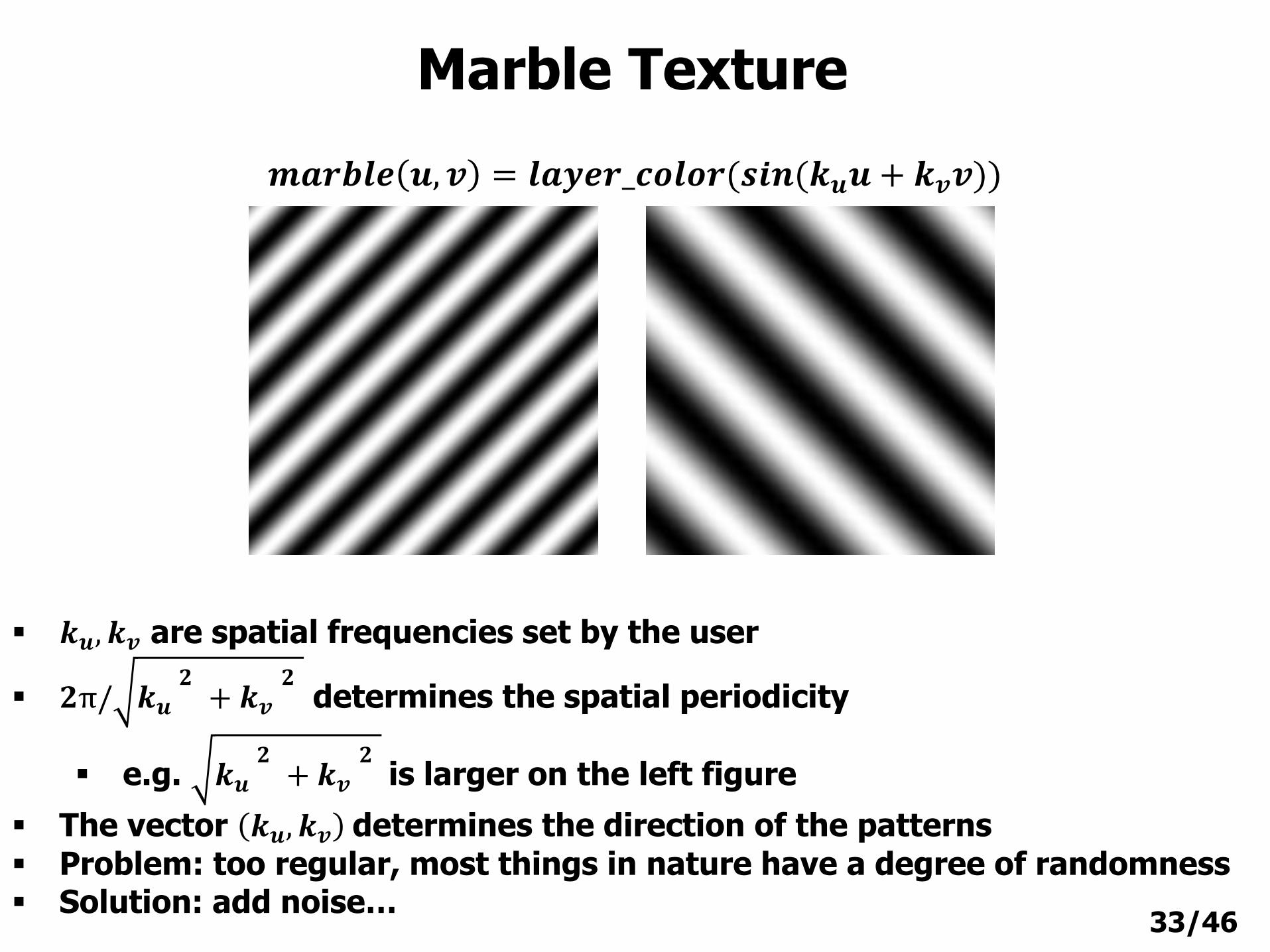
𝒎𝒂𝒓𝒃𝒍𝒆 𝒖, 𝒗 = 𝒍𝒂𝒚𝒆𝒓_𝒄𝒐𝒍𝒐𝒓(𝒔𝒊𝒏(𝒌𝒖𝒖 + 𝒌𝒗𝒗))

33/46

Marble Texture

𝒌𝒖, 𝒌𝒗 are spatial frequencies set by the user

𝟐π/ 𝒌𝒖𝟐+ 𝒌𝒗

𝟐determines the spatial periodicity

e.g. 𝒌𝒖𝟐+ 𝒌𝒗

𝟐is larger on the left figure

The vector 𝒌𝒖, 𝒌𝒗 determines the direction of the patterns

Problem: too regular, most things in nature have a degree of randomness Solution: add noise…

𝒎𝒂𝒓𝒃𝒍𝒆 𝒖, 𝒗 = 𝒍𝒂𝒚𝒆𝒓_𝒄𝒐𝒍𝒐𝒓(𝒔𝒊𝒏(𝒌𝒖𝒖 + 𝒌𝒗𝒗))

34/46

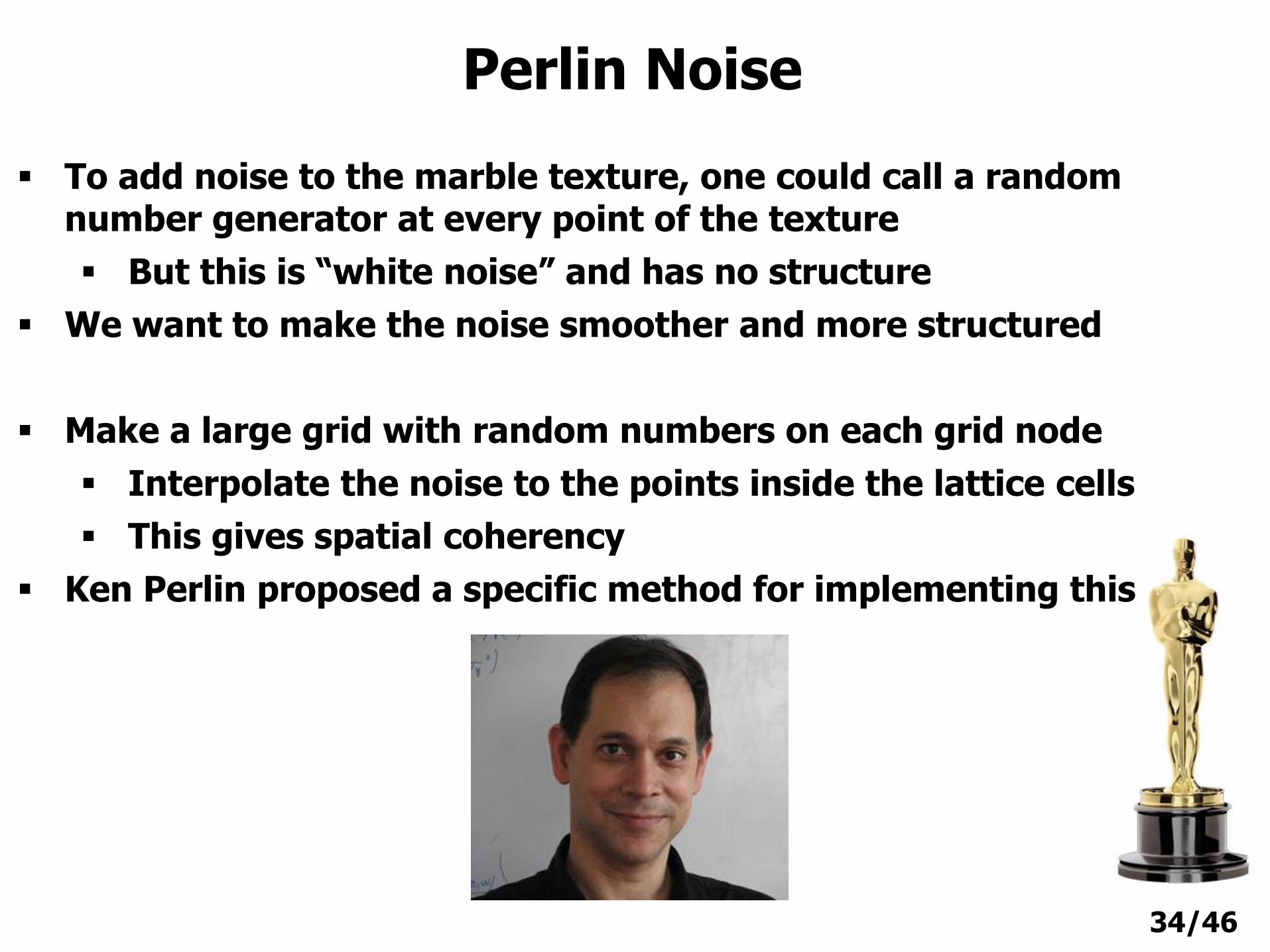
To add noise to the marble texture, one could call a random number generator at every point of the texture

But this is “white noise” and has no structure

We want to make the noise smoother and more structured

Make a large grid with random numbers on each grid node

Interpolate the noise to the points inside the lattice cells

This gives spatial coherency

Ken Perlin proposed a specific method for implementing this

Perlin Noise

35/46

𝒈(𝒖𝟎, 𝒗𝟏)

𝒈(𝒖𝟏, 𝒗𝟏)

𝒈(𝒖𝟎, 𝒗𝟎)

𝒈(𝒖𝟏, 𝒗𝟎)

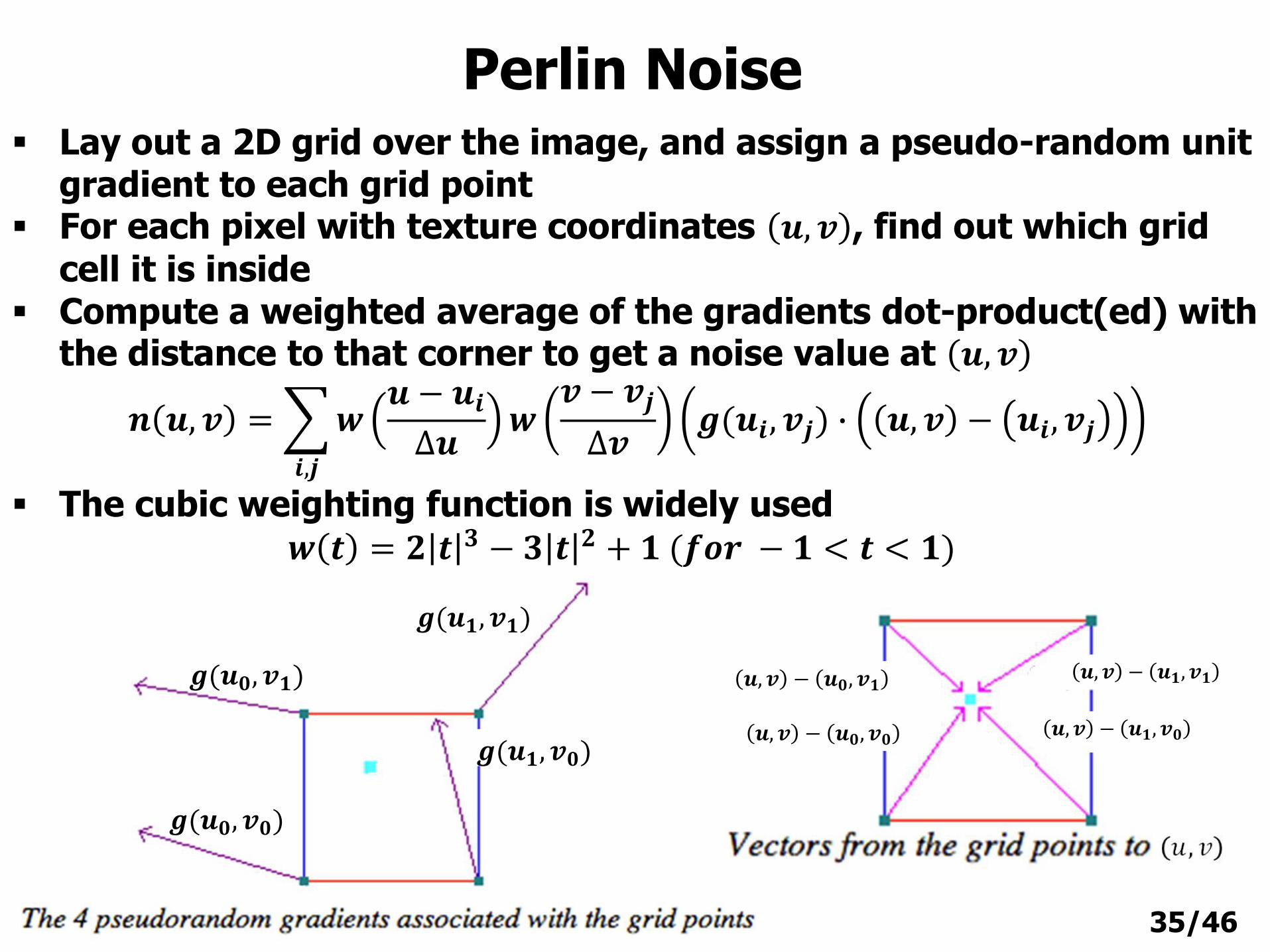
Lay out a 2D grid over the image, and assign a pseudo-random unit gradient to each grid point

For each pixel with texture coordinates 𝒖, 𝒗 , find out which grid

cell it is inside Compute a weighted average of the gradients dot-product(ed) with

the distance to that corner to get a noise value at 𝒖, 𝒗

𝒏 𝒖, 𝒗 =

𝒊,𝒋

𝒘𝒖 − 𝒖𝒊∆𝒖

𝒘𝒗 − 𝒗𝒋

∆𝒗𝒈(𝒖𝒊, 𝒗𝒋) ∙ 𝒖, 𝒗 − 𝒖𝒊, 𝒗𝒋

The cubic weighting function is widely used𝒘 𝒕 = 𝟐 𝒕 𝟑 − 𝟑 𝒕 𝟐 + 𝟏 (𝒇𝒐𝒓 − 𝟏 < 𝒕 < 𝟏)

Perlin Noise

𝒖, 𝒗 − 𝒖𝟎, 𝒗𝟏

𝒖, 𝒗 − 𝒖𝟎, 𝒗𝟎

𝒖, 𝒗 − 𝒖𝟏, 𝒗𝟏

𝒖, 𝒗 − 𝒖𝟏, 𝒗𝟎

36/46

Perlin Noise

Many natural textures contain a variety of feature sizes in the same texture.

The Perlin Noise function recreates this by adding up noises with different frequencies and amplitudes

𝒑𝒆𝒓𝒍𝒊𝒏 𝒖, 𝒗 =

𝒌

𝒏 𝒇𝒓𝒆𝒒𝒖𝒆𝒏𝒄𝒚 𝒌 ∗ 𝒖, 𝒗 ∗ 𝒂𝒎𝒑𝒍𝒊𝒕𝒖𝒅𝒆 𝒌

Typically, frequencies and amplitudes are chosen via

𝒇𝒓𝒆𝒒𝒖𝒆𝒏𝒄𝒚 𝒌 = 𝟐𝒌

𝒂𝒎𝒑𝒍𝒊𝒕𝒖𝒅𝒆 𝒌 = 𝒑𝒆𝒓𝒔𝒊𝒔𝒕𝒆𝒏𝒄𝒆𝒌

Each successive noise function we add is called an octave, because it is twice the frequency of the previous one

Persistence is a parameter (≤ 𝟏) diminishing the relative amplitudes of higher frequencies

37/46

Perlin Noise

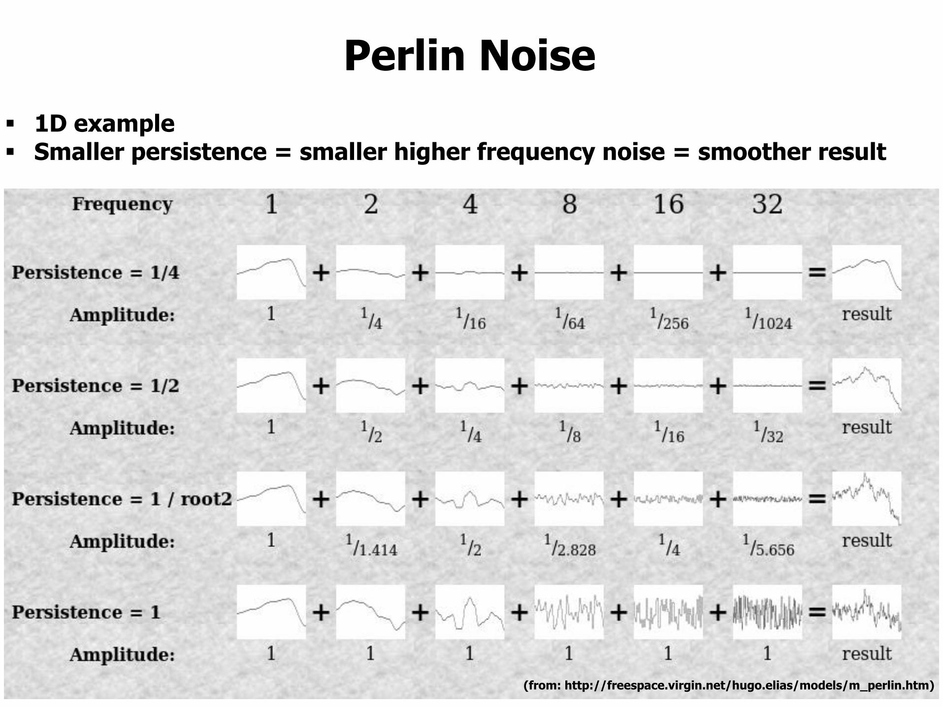
1D example Smaller persistence = smaller higher frequency noise = smoother result

(from: http://freespace.virgin.net/hugo.elias/models/m_perlin.htm)

38/46

Perlin Noise

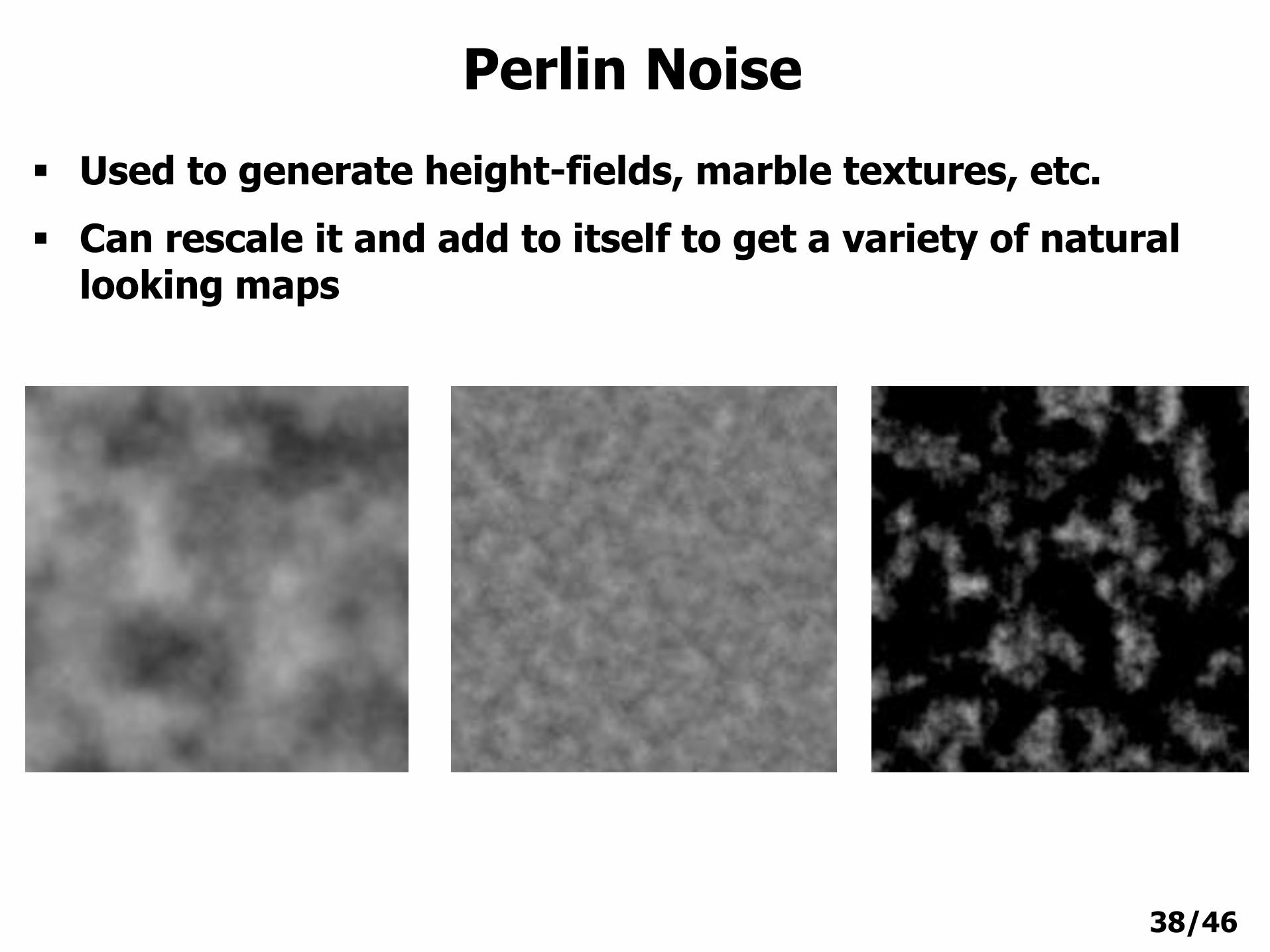
Used to generate height-fields, marble textures, etc.

Can rescale it and add to itself to get a variety of natural looking maps

39/46

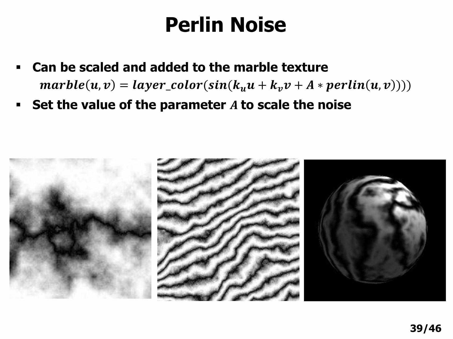
Can be scaled and added to the marble texture

Set the value of the parameter 𝑨 to scale the noise

Perlin Noise

𝒎𝒂𝒓𝒃𝒍𝒆 𝒖, 𝒗 = 𝒍𝒂𝒚𝒆𝒓_𝒄𝒐𝒍𝒐𝒓(𝒔𝒊𝒏(𝒌𝒖𝒖 + 𝒌𝒗𝒗 + 𝑨 ∗ 𝒑𝒆𝒓𝒍𝒊𝒏 𝒖, 𝒗 )))

40/46

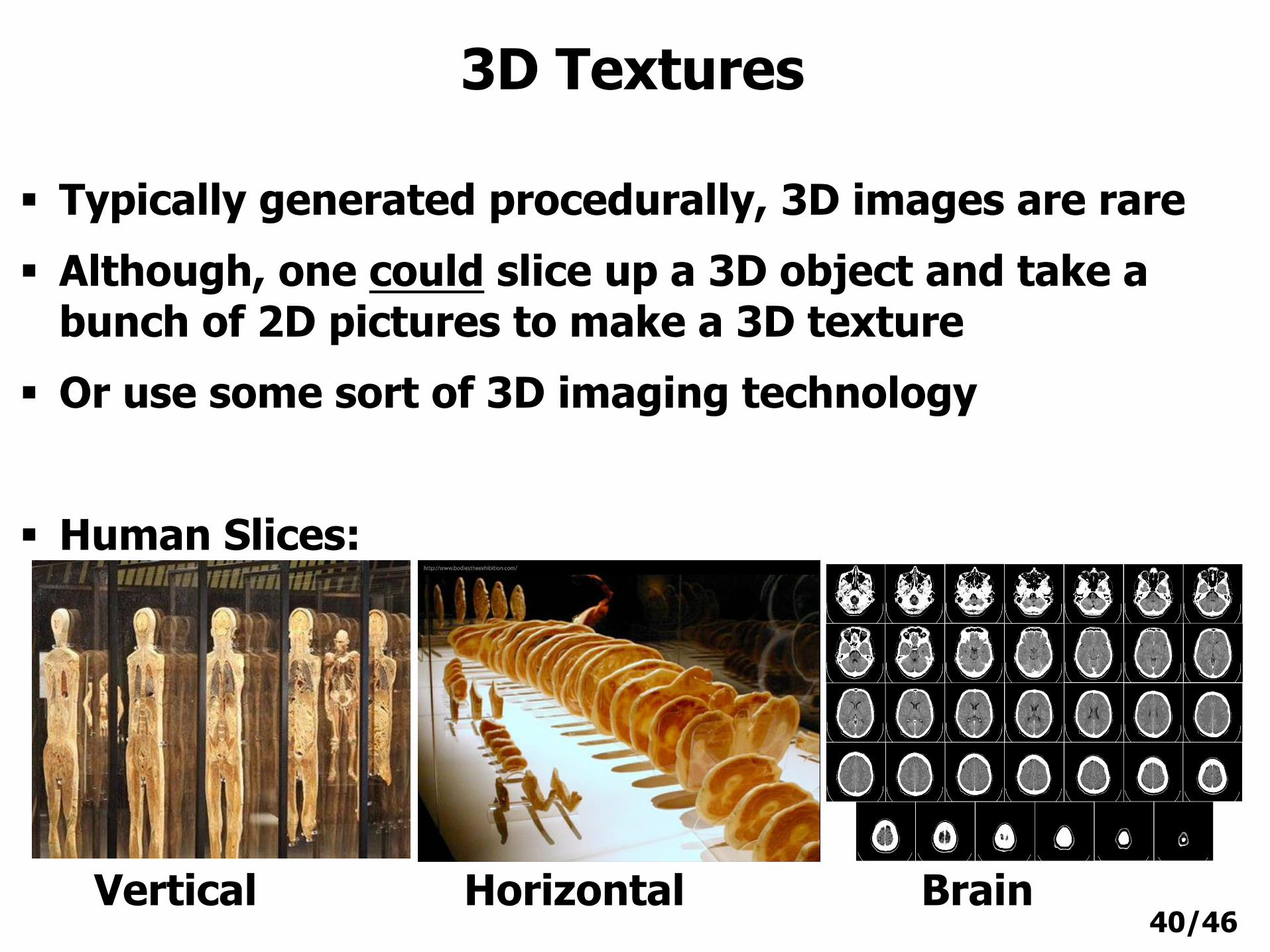
3D Textures

Typically generated procedurally, 3D images are rare

Although, one could slice up a 3D object and take a bunch of 2D pictures to make a 3D texture

Or use some sort of 3D imaging technology

Human Slices:

Vertical Horizontal Brain

41/46

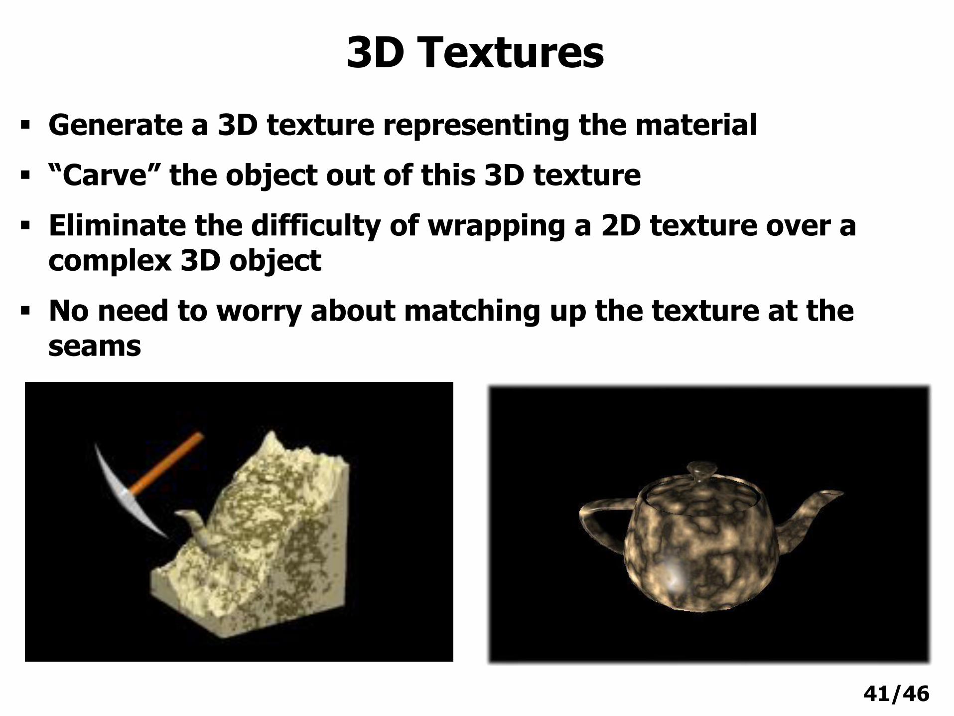
3D Textures

Generate a 3D texture representing the material

“Carve” the object out of this 3D texture

Eliminate the difficulty of wrapping a 2D texture over a complex 3D object

No need to worry about matching up the texture at the seams

42/46

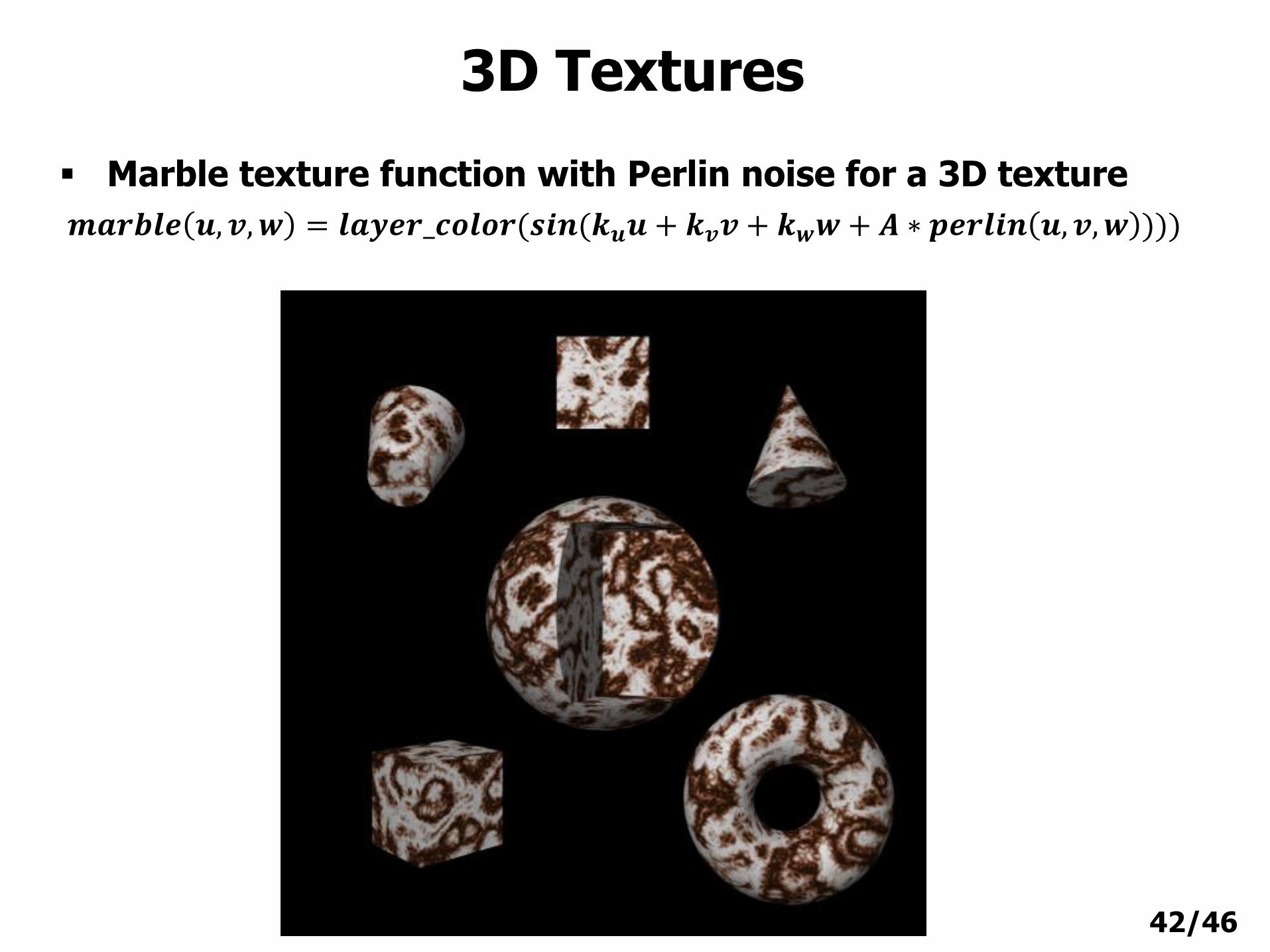
Marble texture function with Perlin noise for a 3D texture

𝒎𝒂𝒓𝒃𝒍𝒆 𝒖, 𝒗,𝒘 = 𝒍𝒂𝒚𝒆𝒓_𝒄𝒐𝒍𝒐𝒓(𝒔𝒊𝒏(𝒌𝒖𝒖 + 𝒌𝒗𝒗 + 𝒌𝒘𝒘+ 𝑨 ∗ 𝒑𝒆𝒓𝒍𝒊𝒏 𝒖, 𝒗,𝒘 )))

3D Textures

43/46

3D Textures

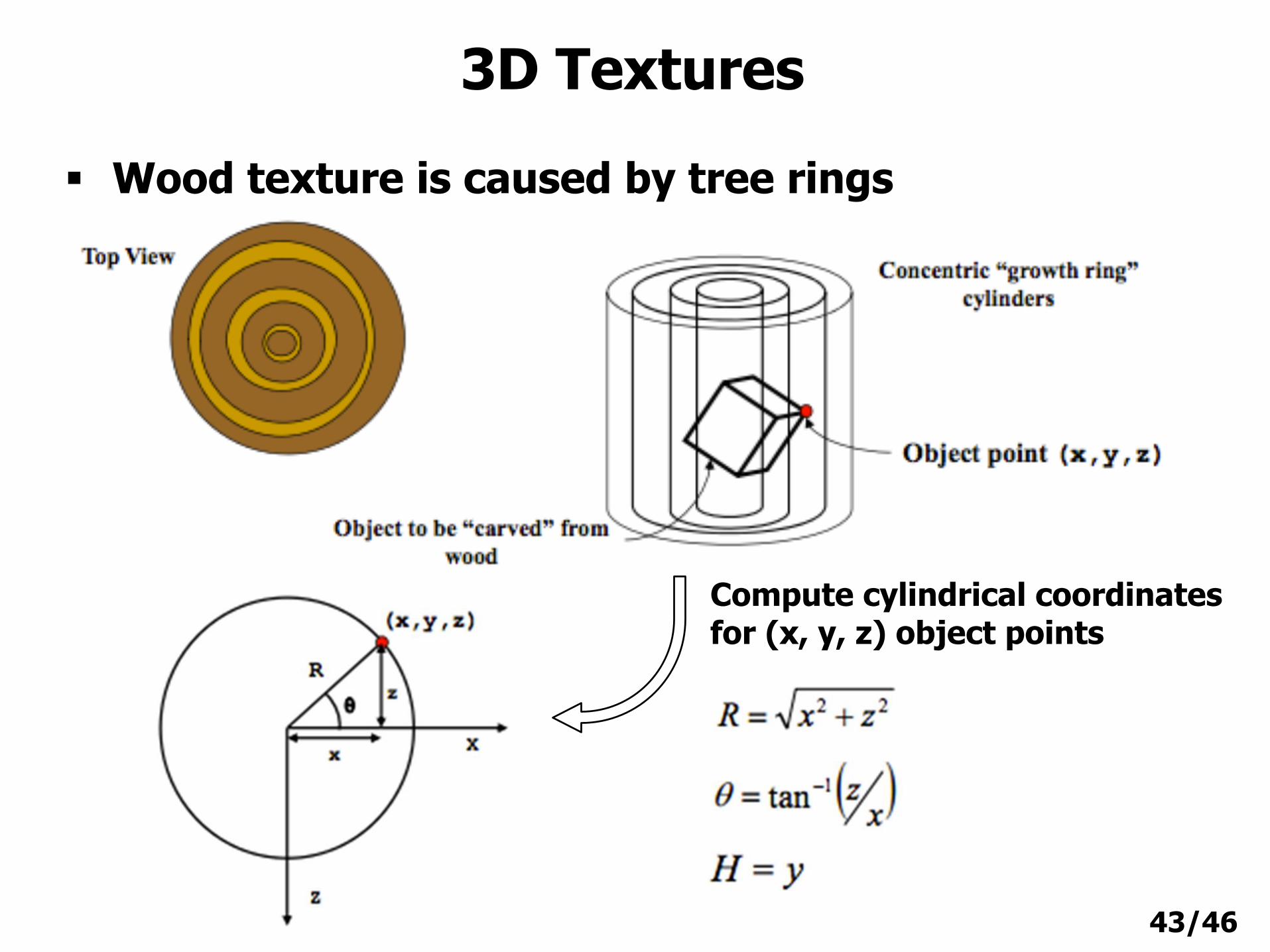
Wood texture is caused by tree rings

Compute cylindrical coordinates for (x, y, z) object points

44/46

3D Textures

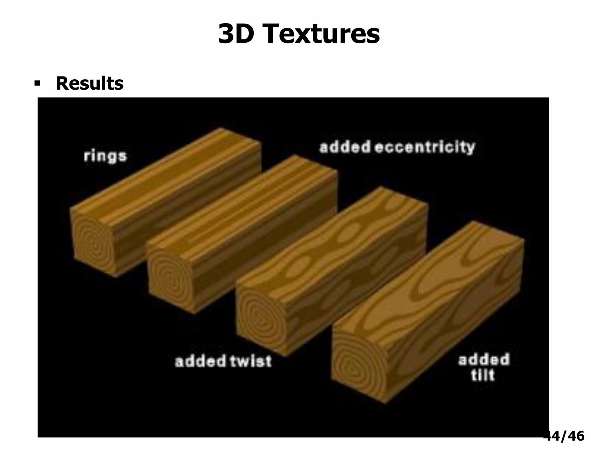
Results

45/46

Texture MappingHomework Tip

46/46

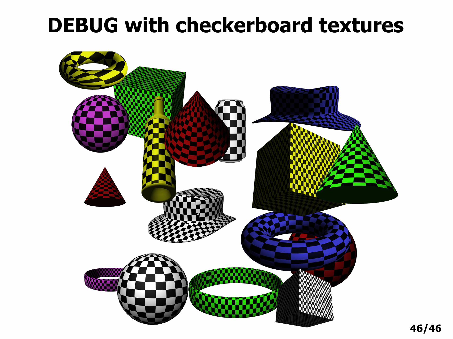
DEBUG with checkerboard textures