morse theory on spaces of braids and lagrangian dynamics
TRANSCRIPT

DOI: 10.1007/s00222-002-0277-0Invent. math. 152, 369–432 (2003)
Morse theory on spaces of braidsand Lagrangian dynamics
R.W. Ghrist1, J.B. Van den Berg2,3, R.C. Vandervorst3 ,4
1 Department of Mathematics, University of Illinois, Urbana, IL 61801, USA2 Department of Applied Mathematics, University of Nottingham, UK3 Department of Mathematics, Free University Amsterdam, De Boelelaan 1081, Amster-
dam, Netherlands4 CDSNS, Georgia Institute of Technology, Atlanta, GA 30332-0160, USA
Oblatum 11-V-2001 & 13-XI-2002Published online: 24 February 2003 – Springer-Verlag 2003
Abstract. In the first half of the paper we construct a Morse-type theory oncertain spaces of braid diagrams. We define a topological invariant of closedpositive braids which is correlated with the existence of invariant sets ofparabolic flows defined on discretized braid spaces. Parabolic flows, a typeof one-dimensional lattice dynamics, evolve singular braid diagrams in sucha way as to decrease their topological complexity; algebraic lengths decreasemonotonically. This topological invariant is derived from a Morse-Conleyhomotopy index.
In the second half of the paper we apply this technology to second orderLagrangians via a discrete formulation of the variational problem. Thisculminates in a very general forcing theorem for the existence of infinitelymany braid classes of closed orbits.
1. Prelude
It is well-known that under the evolution of any scalar uniformly parabolicequation of the form
ut = f(x, u, ux, uxx) ; ∂uxx f ≥ δ > 0,(1)
the graphs of two solutions u1(x, t) and u2(x, t) evolve in such a waythat the number of intersections of the graphs does not increase in time.
The first author was supported by NSF DMS-9971629 and NSF DMS-0134408. Thesecond author was supported by an EPSRC Fellowship. The third author was supported byNWO Vidi-grant 639.032.202.

370 R.W. Ghrist et al.
This principle, known in various circles as “comparison principle” or “lapnumber” techniques, entwines the geometry of the graphs (uxx is a curvatureterm), the topology of the solutions (the intersection number is a local linkingnumber), and the local dynamics of the PDE. This is a valuable approachfor understanding local dynamics for a wide variety of flows exhibitingparabolic behavior with both classical [54] and contemporary [41,5,10,19]implications.
This paper is an extension of this local technique to a global technique.One such well-established globalization appears in the work of Angenenton curve-shortening [4]: evolving closed curves on a surface by curve short-ening isolates the classes of curves dynamically and implies a monotonicitywith respect to number of self-intersections.
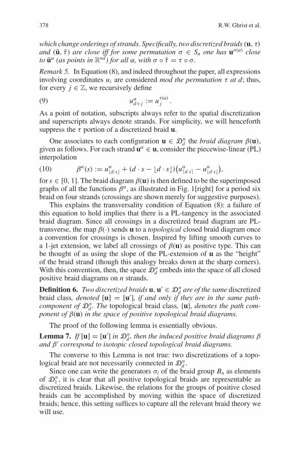
In contrast, one could consider the following topological globalization.Superimposing the graphs of a collection of functions uα(x) gives some-thing which resembles the projection of a topological braid onto the plane.Assume that the “height” of the strands above the page is given by theslope uα
x (x), or, equivalently, that all of the crossings in the projection are ofthe same sign (bottom-over-top): see Fig. 1[left]. Evolving these functionsunder a parabolic equation (with, say, boundary endpoints fixed) yieldsa flow on a certain space of braid diagrams which has a topological mono-tonicity: linking can be destroyed but not created. This establishes a partialordering on the semigroup of positive braids which is respected by parabolicdynamics. The idea of topological braid classes with this partial ordering isa globalization of the lap number (which, in braid-theoretic terms becomesthe length of the braid in the braid group under standard generators).
1.1. Parabolic flows on spaces of braid diagrams. In this paper, we initi-ate the study of parabolic flows on spaces of braid diagrams. The particularbraids in question will be (a) positive – all crossings are considered to be ofthe same sign; (b) closed1 – the left and right sides are identified; and (c) dis-cretized – or piecewise linear with fixed distance between “anchor points,”so as to avoid the analytic difficulties of working on infinite dimensionalspaces of curves. See Fig. 1 for examples of braid diagrams.
u
xx x
u u
ux
Fig. 1. Curves in the x–u plane [left] lift to a braid [center] which is then discretized [right].In a discretized isotopy, one slides the anchor points vertically
1 The theory works equally well for braids with fixed endpoints.

Morse theory on spaces of braids 371
The flows we consider evolve the anchor points of the braid diagram sothat the braid class can change, but only so as to decrease complexity: locallinking of strands may not increase with time. Due to the close similaritywith parabolic partial differential equations such systems will be referred toas parabolic recurrence relations, and the induced flows as parabolic flows.These flows are given by
d
dtui = Ri(ui−1, ui, ui+1),(2)
where the variables ui represent the vertical positions of the ordered anchorpoints of discrete braid diagrams. The only conditions imposed on the dy-namics is the monotonicity condition that every Ri be increasing functionsof ui−1 and ui+1.
While a discretization of a PDE of the form (1) with nearest-neighborinteraction yields a parabolic recurrence relation, the class of dynamics weconsider is significantly larger in scope (see, e.g., [40]). Parabolic recurrencerelations are a sub-class of monotone recurrence relations as studied in [3]and [26].
The evolution of braid diagrams yields a situation not unlike that con-sidered by Vassiliev in knot theory [59]: in our scenario, the space of allbraid diagrams is partitioned by the discriminant of singular diagrams intothe braid classes. The parabolic flows we consider are transverse to thesesingular varieties (except for a set of “collapsed” braids) and are co-orientedin a direction along which the algebraic length of the braid decreases: thisis an algebraic version of curve shortening.
To proceed, two types of noncompactness on spaces of braid diagramsmust be repaired. Most severe is the problem of braid strands completelycollapsing onto one another. To resolve this type of noncompactness, weassume that the dynamics fixes some collection of braid strands, a skeleton,and then work on spaces of braid pairs: one free, one fixed. The relativetheory then leads to forcing results of the type “Given a stationary braidclass, which other braids are forced as invariant sets of parabolic flows?”The second type of noncompactness in the dynamics occurs when the braidstrands are free to evolve to arbitrarily large values. In the PDE setting, onerequires knowledge of boundary conditions at infinity to prove theoremsabout the dynamics. In our braid-theoretic context, we convert boundaryconditions to “artificial” braid strands augmented to the fixed skeleton.
Thus, working on spaces of braid pairs, the dynamics at the discrimi-nant permits the construction of a Morse theory in the spirit of Conley todetect invariant sets of parabolic flows. Conley’s extension of the Morseindex associates to any sufficiently isolated invariant set a space whosehomotopy type measures not merely the dimension of the unstable mani-fold (the Morse index) but rather the coarse topological features of theunstable dynamics associated to this set. We obtain a well-defined Con-ley index for braid diagrams from the monotonicity properties of parabolic

372 R.W. Ghrist et al.
flows. To be more precise, relative braid classes (equivalence classes of iso-topic braid diagrams fixing some skeleton) serve as candidates for isolatingneighborhoods to which the Conley index can be assigned. This approach isreminiscent of the ideas of linking of periodic orbits used by Angenent [2,4]and LeCalvez [36,37].
Our finite-dimensional approximations to the (infinite-dimensional)space of smooth topological braids conceivably alter the Morse-theoreticproperties of the discretized braid classes. One would like to know that solong as the discretization is not degenerately coarse, the homotopy indexis independent of both the discretization and the specific parabolic flowemployed. This is true. The principal topological result of this work is thatthe homotopy index is indeed an invariant of the topological (relative) braidclass: see Theorems 19 and 20 for details. These theorems seem to evadea simple algebraic-topological proof. The proof we employ in Sect. 5 con-structs the appropriate homotopy by recasting the problem into singulardynamics and applying techniques from singular perturbation theory.
We thus obtain a topological index which can, like the Morse index,force the existence of invariant sets. Specifically, a non-vanishing homotopyindex for a relative braid class indicates that there is an invariant set in thisbraid class for any parabolic flow with the appropriate skeleton. This is thefoundation for the applications to follow in the remainder of the paper.
The remainder of the paper explores applications of the machinery toa broad class of Lagrangian dynamics.
1.2. Second order Lagrangian dynamics. Our principal application ofthe Morse theory on discretized braids is to the problem of finding periodicorbits of second order Lagrangian systems: that is, Lagrangians of the formL(u, ux, uxx) where L ∈ C2(R3). An important motivation for studyingsuch systems comes from the stationary Swift-Hohenberg model in physics,which is described by the fourth order equation
(1+ d2
dx2
)2
u − αu + u3 = 0, α ∈ R.(3)
This equation is the Euler-Lagrange equation of the second order Lagrangian
L(u, ux, uxx) = 1
2|uxx|2 − |ux |2 + 1− α
2u2 + 1
4u4.(4)
We generalize to the broadest possible class of second order Lagrangians.One begins with the conventional convexity assumption, ∂2
wL(u, v,w) ≥δ > 0. The objective is to find bounded functions u : R → R which arestationary for the action integral J[u] := ∫
L(u, ux, uxx)dx. Such functionsu are bounded solutions of the Euler-Lagrange equations
d2
dx2
∂L
∂uxx− d
dx
∂L
∂ux+ ∂L
∂u= 0.(5)

Morse theory on spaces of braids 373
Due to the translation invariance x → x + c, the solutions of (5) satisfy theenergy constraint(
∂L
∂ux− d
dx
∂L
∂uxx
)ux + ∂L
∂uxxuxx − L(u, ux, uxx) = E = constant,(6)
where E is the energy of a solution. To find bounded solutions for givenvalues of E, we employ the variational principle δu,T
∫ T0
(L(u, ux, uxx) +
E)dx = 0, which forces solutions of (5) to have energy E. The Lagrangian
problem can be reformulated as a two degree-of-freedom Hamiltonian sys-tem; in that context, bounded periodic solutions are closed characteristicsof the (corresponding) energy manifold M3 ⊂ R4. Unlike the case of first-order Lagrangian systems, the energy hypersurface is not of contact typein general [6], and the recent stunning results in contact homology [16] areinapplicable.
The variational principle can be discretized for a certain considerableclass of second order Lagrangians: those for which monotone laps betweenconsecutive extrema ui are unique and continuous with respect to the end-points. We give a precise definition in Sect. 8, denoting these as (second orderLagrangian) twist systems. Due to the energy identity (6) the extrema ui arerestricted to the set UE = u | L(u, 0, 0)+ E ≥ 0, connected componentsof which are called interval components and denoted by IE . An energy levelis called regular if ∂L
∂u (u, 0, 0) = 0 for all u satisfying L(u, 0, 0)+E = 0. Inorder to deal with non-compact interval components IE certain asymptoticbehavior has to be specified, for example that “infinity” is attracting. SuchLagrangians are called dissipative, and are most common in models comingfrom physics, like the Swift-Hohenberg Lagrangian. For a precise definitionof dissipativity see Sect. 9. Other asymptotic behaviors may be consideredas well, such as “infinity” is repelling, or more generally that infinity isisolating, implying that closed characteristics are a priori bounded in L∞.
Closed characteristics are either simple or non-simple depending onwhether u(x), represented as a closed curve in the (u, ux)-plane, is a simpleclosed curve or not. This distinction is a sufficient language for the followinggeneral forcing theorem:
Theorem 1. Any dissipative twist system possessing a non-simple closedcharacteristic u(x) at a regular energy value E such that u(x) ∈ IE, mustpossess an infinite number of (non-isotopic) closed characteristics at thesame energy level as u(x).
This is the optimal type of forcing result: there are neither hidden as-sumptions about nondegeneracy of the orbits, nor restrictions to generic be-havior. Sharpness comes from the fact that there exist systems with finitelymany simple closed characteristics at each energy level.
The above result raises the following question: when does an energymanifold contain a non-simple closed characteristic? In general the exis-tence of such characteristics depends on the geometry of the energy mani-fold. One geometric property that sparks the existence of non-simple closed

374 R.W. Ghrist et al.
characteristics is a singularity or near-singularity of the energy manifold.This, coupled with Theorem 1, triggers the existence of infinitely manyclosed characteristics. The results that can be proved in this context (dis-sipative twist systems) give a complete classification with respect to theexistence of finitely many versus infinitely many closed characteristics onsingular energy levels. The first result in this direction deals with singularenergy values for which IE = R.
Theorem 2. Suppose that a dissipative twist system has a singular energylevel E with IE = R, which contains two or more rest points. Then thesystem has infinitely many closed characteristics at energy level E.2
Complementary to the above situation is the case when IE containsexactly one rest point. To have infinitely many closed characteristics, thenature of the rest point will come into play. If the rest point is a center(four imaginary eigenvalues), then the system has infinitely many closedcharacteristics at each energy level sufficiently close to E, including E. Ifthe rest point is not a center, there need not exist infinitely many closedcharacteristics as results in [57] indicate.
Similar results can be proved for compact interval components (forwhich dissipativity is irrelevant) and semi-infinite interval componentsIE R±.
Theorem 3. Suppose that a dissipative twist system has a singular energylevel E with an interval component IE = [a, b], or IE R±, which containsat least one rest point of saddle-focus/center type. Then the system hasinfinitely many closed characteristics at energy level E.
If an interval component contains no rest points, or only degeneraterest points (0 eigenvalues), then there need not exist infinitely many closedcharacteristics, completing our classification.
This classification immediately applies to the Swift-Hohenbergmodel (3), which is a twist system for all parameter values α ∈ R. Weleave it to the reader to apply the above theorems to the different regimesof α.
1.3. Additional applications. The framework of parabolic recurrence re-lations that we construct is robust enough to accommodate several otherimportant classes of dynamics.
1.3.1. First-order nonautonomous Lagrangians. Finding periodic solutionsof first-order Lagrangian systems of the form δ
∫L(x, u, ux)dx = 0, with
L being 1-periodic in x, can be rephrased in terms of parabolic recurrencerelations of gradient type. The homotopy index can be used to find periodicsolutions u(x) in this setting, even though a globally defined Poincare mapon R2 need not exist.
2 From the proof of this theorem in Sect. 9 it follows that the statement remains true forenergy values E + c, with c > 0 small.

Morse theory on spaces of braids 375
1.3.2. Monotone twist maps. A monotone twist map (compare [3,48]) is a(not necessarily area-preserving) map on R2 of the form
(u, pu)→ (u′, p′u),∂u′
∂pu> 0.
Periodic orbits (ui, pui ) are found by solving a parabolic recurrence rela-tion for the u-coordinates derived from the twist property.
1.3.3. Uniformly parabolic PDE’s. The study of the invariant dynamicsof Equation (1) can also be formulated in terms of parabolic recurrencerelations by a spatial discretization. The basic theory for braid forcingdeveloped here can be adapted to the dynamics of Equation (1): see [23,24]for details.
1.3.4. Lattice dynamics. The form of a parabolic recurrence relation isprecisely that arising from a set of coupled oscillators on a [periodic] one-dimensional lattice with nearest-neighbor attractive coupling. A similarsetup arises in Aubry-LeDaeron-Mather theory of the Frenkel-Kontorovamodel [7]. In this setting, a nontrivial homotopy index yields existenceof invariant states (or stationary, in the exact context) within a particularbraid class. Related physical systems (e.g., charge density waves on a 1-dlattice [45]) are also often reducible to parabolic recurrence relations.
1.4. History and outline. The history of our approach is the convergenceof ideas from knot theory, the dynamics of annulus twist maps, and curveshortening. We have already mentioned the similarities with Vassiliev’stopological approach to discriminants in the space of immersed knots. Fromthe dynamical systems perspective, the study of parabolic flows and gradientflows in relation with embedding data and the Conley index can be foundin work of Angenent [2–4] and Le Calvez [36,37] on area preserving twistmaps. More general studies of dynamical properties of parabolic-type flowsappear in numerous works: we have been inspired by the work of Smil-lie [53], Mallet-Paret and Smith [39], Hirsch [26], and, most strongly, thework of Angenent on curve shortening [4]. Many of our applications to find-ing closed characteristics of second order Lagrangian systems share similargoals with the programme of Hofer and his collaborators (see, e.g., [16,27,28]), with the novelty that our energy surfaces are all non-compact and notnecessarily of contact type [6].
Clearly there is a parallel between the homotopy index theory presentedhere and Boyland’s adaptation of Nielsen-Thurston theory for braid typesof surface diffeomorphisms [9]. An important difference is that we requirecompactness only at the level of braid diagrams, which does not yield com-pactness on the level of the domains of the return maps [if these indeedexist]. Another important observation is that the recurrence relations are

376 R.W. Ghrist et al.
sometimes not defined on all of R2, which makes it very hard if not impos-sible to rephrase the problem of finding periodic solutions in terms of fixedpoints of 2-dimensional maps.
There are three components of this paper: (a) the precise definitions ofthe spaces involved and flows constructed, covered in Sects. 2–3; (b) theestablishment of existence, invariance, and properties of the index for braiddiagrams in Sects. 4–7; and (c) applications of the machinery to second orderLagrangian systems Sects. 8–10. Finally, Sect. 11 contains open questionsand remarks.
Acknowledgements. The authors would like express special gratitude to Sigurd Angenentand Konstantin Mischaikow for numerous enlightening discussions. Special thanks to Mad-jid Allili for his computational work in the earliest stages of this work. Finally, the hardwork of the referee has improved the paper in several respects, especially in the definitionsof equivalent relative braid classes.
Contents
1 Prelude . . . . . . . . . . . . . . . . . . . . . . . . . . . . . . . . . . . . . . . 3692 Spaces of discretized braid diagrams . . . . . . . . . . . . . . . . . . . . . . . . 3763 Parabolic recurrence relations . . . . . . . . . . . . . . . . . . . . . . . . . . . . 3804 The homotopy index for discretized braids . . . . . . . . . . . . . . . . . . . . . 3845 Stabilization and invariance . . . . . . . . . . . . . . . . . . . . . . . . . . . . . 3906 Duality . . . . . . . . . . . . . . . . . . . . . . . . . . . . . . . . . . . . . . . . 3997 Morse theory . . . . . . . . . . . . . . . . . . . . . . . . . . . . . . . . . . . . 4028 Second order Lagrangian systems . . . . . . . . . . . . . . . . . . . . . . . . . 4059 Multiplicity of closed characteristics . . . . . . . . . . . . . . . . . . . . . . . . 41110 Computation of the homotopy index . . . . . . . . . . . . . . . . . . . . . . . . 42111 Postlude . . . . . . . . . . . . . . . . . . . . . . . . . . . . . . . . . . . . . . . 425Appendix A. Construction of parabolic flows . . . . . . . . . . . . . . . . . . . . . 428References . . . . . . . . . . . . . . . . . . . . . . . . . . . . . . . . . . . . . . . . 430
2. Spaces of discretized braid diagrams
2.1. Definitions. Recall the definition of a braid (see [8,25] for a compre-hensive introduction). A braid β on n strands is a collection of embeddingsβα : [0, 1] → R3nα=1 with disjoint images such that (a) βα(0) = (0, α, 0);(b) βα(1) = (1, τ(α), 0) for some permutation τ; and (c) the image of eachβα is transverse to all planes x = const. We will “read” braids from left toright with respect to the x-coordinate. Two such braids are said to be of thesame topological braid class if they are homotopic in the space of braids:one can deform one braid to the other without any intersections among thestrands. There is a natural group structure on the space of topological braidswith n strands, Bn, given by concatenation. Using generators σi which in-terchange the i th and (i + 1)st strands (with a positive crossing) yields the

Morse theory on spaces of braids 377
presentation for Bn:
Bn :=⟨σ1, . . . , σn−1 : σiσ j = σ jσi ; |i − j| > 1
σiσi+1σi = σi+1σiσi+1 ; i < n − 1
⟩.(7)
Braids find their greatest applications in knot theory via taking theirclosures. Algebraically, the closed braids on n strands can be defined as theset of conjugacy classes3 in Bn. Geometrically, one quotients out the rangeof the braid embeddings via the equivalence relation (0, y, z) ∼ (1, y, z)and alters the restriction (a) and (b) of the position of the endpoints to beβα(0) ∼ βτ(α)(1), as in Fig. 1[center]. Thus, a closed braid is a collectionof disjoint embedded loops in S1 × R2 which are everywhere transverse tothe R2-planes.
The specification of a topological braid class (closed or otherwise) maybe accomplished unambiguously by a labeled projection to the (x, y)-plane:a braid diagram. Any braid may be perturbed slightly so that pairs of strandcrossings in the projection are transversal: in this case, a marking of (+)or (−) serves to indicate whether the crossing is “bottom over top” or “topover bottom” respectively. Fig. 1[center] illustrates a topological braid withall crossings positive.
2.2. Discretized braids. In the sequel we will restrict to a class of closedbraid diagrams which have two special properties: (a) they are positive – thatis, all crossings are of (+) type; and (b) they are discretized, or piecewiselinear diagrams with constraints on the positions of anchor points. Weparameterize such diagrams by the configuration space of anchor points.
Definition 4. The space of discretized period d braids on n strands, denotedDn
d , is the space of all pairs (u, τ) where τ ∈ Sn is a permutation onn elements, and u is an unordered collection of n strands, u = uαnα=1,satisfying the following conditions:
(a) Each strand consists of d + 1 anchor points: uα = (uα0 , uα
1 , . . . , uαd )
∈ Rd+1.(b) For all α = 1, . . . , n, one has
uαd = uτ(α)
0 .
(c) The following transversality condition is satisfied: for any pair of dis-tinct strands α and α′ such that uα
i = uα′i for some i,(
uαi−1 − uα′
i−1
)(uα
i+1 − uα′i+1
)< 0.(8)
The topology on Dnd is the standard topology of Rnd on the strands and the
discrete topology with respect to the permutation τ , modulo permutations
3 Note that we fix the number of strands and do not allow the Markov move commonlyused in knot theory.
378 R.W. Ghrist et al.
which change orderings of strands. Specifically, two discretized braids (u, τ)and (u, τ) are close iff for some permutation σ ∈ Sn one has uσ(α) closeto uα (as points in Rnd) for all α, with σ τ = τ σ .
Remark 5. In Equation (8), and indeed throughout the paper, all expressionsinvolving coordinates ui are considered mod the permutation τ at d; thus,for every j ∈ Z, we recursively define
uαd+ j := uτ(α)
j .(9)
As a point of notation, subscripts always refer to the spatial discretizationand superscripts always denote strands. For simplicity, we will henceforthsuppress the τ portion of a discretized braid u.
One associates to each configuration u ∈ Dnd the braid diagram β(u),
given as follows. For each strand uα ∈ u, consider the piecewise-linear (PL)interpolation
βα(s) := uαd·s + (d · s − d · s )(uα
d·s − uαd·s
),(10)
for s ∈ [0, 1]. The braid diagram β(u) is then defined to be the superimposedgraphs of all the functions βα, as illustrated in Fig. 1[right] for a period sixbraid on four strands (crossings are shown merely for suggestive purposes).
This explains the transversality condition of Equation (8): a failure ofthis equation to hold implies that there is a PL-tangency in the associatedbraid diagram. Since all crossings in a discretized braid diagram are PL-transverse, the map β(·) sends u to a topological closed braid diagram oncea convention for crossings is chosen. Inspired by lifting smooth curves toa 1-jet extension, we label all crossings of β(u) as positive type. This canbe thought of as using the slope of the PL-extension of u as the “height”of the braid strand (though this analogy breaks down at the sharp corners).With this convention, then, the space Dn
d embeds into the space of all closedpositive braid diagrams on n strands.
Definition 6. Two discretized braids u, u′ ∈ Dnd are of the same discretized
braid class, denoted [u] = [u′], if and only if they are in the same path-component of Dn
d . The topological braid class, u, denotes the path com-ponent of β(u) in the space of positive topological braid diagrams.
The proof of the following lemma is essentially obvious.
Lemma 7. If [u] = [u′] in Dnd , then the induced positive braid diagrams β
and β′ correspond to isotopic closed topological braid diagrams.
The converse to this Lemma is not true: two discretizations of a topo-logical braid are not necessarily connected in Dn
d .Since one can write the generators σi of the braid group Bn as elements
of Dn1 , it is clear that all positive topological braids are representable as
discretized braids. Likewise, the relations for the groups of positive closedbraids can be accomplished by moving within the space of discretizedbraids; hence, this setting suffices to capture all the relevant braid theory wewill use.
Morse theory on spaces of braids 379
2.3. Singular braids. The appropriate discriminant for completing thespace Dn
d consists of those “singular” braid diagrams admitting tangen-cies between strands.
Definition 8. Denote by Dnd the nd-dimensional vector space4 of all dis-
cretized braid diagrams u which satisfy properties (a) and (b) of Definition 4.Denote by Σn
d := Dnd −Dn
d the set of singular discretized braids.
We will often suppress the period and strand data and write Σ forthe space of singular discretized braids. It follows from Definition 4 andEquation (8) that the set Σn
d is a semi-algebraic variety in Dnd . Specifically,
for any singular braid u ∈ Σ there exists an integer i ∈ 1, . . . , d andindices α = α′ such that uα
i = uα′i , and
(uα
i−1 − uα′i−1
)(uα
i+1 − uα′i+1
) ≥ 0,(11)
where the subscript is always computed mod the permutation τ at d. Thenumber of such distinct occurrences is the codimension of the singular braiddiagram u ∈ Σ. We decompose Σ into the union of strata Σ[m] graded bym, the codimension of the singularity.
Any closed braid (discretized or topological) is partitioned into compo-nents by the permutation τ . Geometrically, the components are preciselythe connected components of the closed braid diagram. In our context,a component of a discretized braid can be specified as uα
i i∈Z, since, by ourindexing convention, i “wraps around” to the other side of the braid wheni ∈ 1, . . . , d.
For singular braid diagrams of sufficiently high codimension, entire com-ponents of the braid diagram can coalesce. This can happen in essentiallytwo ways: (1) a single component involving multiple strands can collapseinto a braid with fewer numbers of strands, or (2) distinct components cancoalesce into a single component. We define the collapsed singularities,Σ−, as follows:
Σ− := u ∈ Σ
∣∣ uαi = uα′
i , ∀i ∈ Z, for some α = α′ ⊂ Σ.
Clearly the codimension of singularities in Σ− is at least d. Since for braiddiagrams in Σ− the number of strands reduces, the subspace Σ− may bedecomposed into a union of the spaces Dn′
d for n′ < n; i.e., Σ− = ∪n′<nDn′d .
If n = 1, then Σ− = ∅.
2.4. Relative braid classes. Evolving certain components of a braid dia-gram while fixing the remaining components motivates working with a classof “relative” braid diagrams.
4 Strictly speaking Dnd is not a vector space, but a union of vector spaces. Fixing appro-
priate permutations its components are vector spaces. Consider for instance D31 which is
a union of 3 copies of R3.
380 R.W. Ghrist et al.
Given u ∈ Dnd and v ∈ Dm
d , the union u∪v ∈ Dn+md is naturally defined
as the unordered union of the strands. Given v ∈ Dmd , define
Dnd REL v :=
u ∈ Dnd : u ∪ v ∈ Dn+m
d
,
fixing v and imposing transversality. The path components of Dnd REL v
comprise the relative discrete braid classes, denoted [u REL v]. The braidv will be called the skeleton henceforth. The set of singular braids Σ REL vare those braids u such that u ∪ v ∈ Σn+m
d . The collapsed singular braidsare denoted by Σ− REL v. As before, the set (Dn
d REL v) ∪ (Σ REL v)
is the closure of Dnd REL v in Rnd, and is denoted Dn
d REL v. We denoteby u REL v the topological relative braid class: the set of topological(positive, closed) braids u such that u∪ v is a topological (positive, closed)braid diagram.
Given two relative braid classes [u REL v] and [u′ REL v′] in Dnd REL v
and Dnd REL v′ respectively, to what extend are they the same? Consider the
set
D = (u, v) ∈ Dn
d ×Dmd
∣∣ u ∪ v ∈ Dn+md
.
The natural projection π : (u, v) → v from D to Dmd has as its fiber the
braid class [u REL v]. The path component of (u, v) in D will be denoted[u REL [v]]. This generates the equivalence relation for relative braid classes
to be used in the remainder of this work: [u REL v] ∼ [u′ REL v′] if andonly if
[u REL [v]] = [
u′ REL [v′]].Likewise, define
u REL v to be the set of equivalent topological
relative braid classes. That is, u REL v ∼ u′ REL v′ if and only if thereis a continuous family of topological (positive, closed) braid diagram pairsdeforming (u, v) to (u′, v′).
3. Parabolic recurrence relations
We consider the dynamics of vector fields given by recurrence relationson the spaces of discretized braid diagrams. These recurrence relations arenearest neighbor interactions – each anchor point on a braid strand influencesanchor points to the immediate left and right on that strand – and resemblespatial discretizations of parabolic equations.
3.1. Axioms and exactness. Denote by X the sequence space X := RZ.
Definition 9. A parabolic recurrence relation R on X is a sequence ofreal-valued C1 functions R = (Ri)i∈Z satisfying
(A1): [monotonicity]5 ∂1Ri > 0 and ∂3Ri ≥ 0 for all i ∈ Z(A2): [periodicity] For some d ∈ N, Ri+d = Ri for all i ∈ Z.
5 Equivalently, one could impose ∂1Ri ≥ 0 and ∂3Ri > 0 for all i.

Morse theory on spaces of braids 381
For applications to Lagrangian dynamics a variational structure is ne-cessary. At the level of recurrence relations this implies that R is a gradient:
Definition 10. A parabolic recurrence relation on X is called exact if
(A3): [exactness] There exists a sequence of C2 generating functions,(Si)i∈Z, satisfying
Ri(ui−1, ui, ui+1) = ∂2Si−1(ui−1, ui)+ ∂1Si(ui, ui+1),(12)
for all i ∈ Z.
In discretized Lagrangian problems the action functional naturally de-fines the generating functions Si. This agrees with the “formal” action inthis case: W(u) :=∑
i Si(ui, ui+1). In this general setting, R = ∇W .
3.2. The induced flow. In order to define parabolic flows we regard R asa vector field on X: consider the differential equations
d
dtui = Ri(ui−1, ui, ui+1), u(t) ∈ X, t ∈ R.(13)
Equation (13) defines a (local) C1 flow ψt on X under any periodic boundaryconditions with period nd. To define flows on the finite dimensional spacesDn
d , one considers the same equations:
d
dtuα
i = Ri(uα
i−1, uαi , uα
i+1
), u ∈ Dn
d .(14)
where the ends of the braids are identified as per Remark 5. Axiom (A2)guarantees that the flow is well-defined. Indeed, one may consider a coverof Dn
d by taking the bi-infinite periodic extension of the braids: this yieldsa subspace of periodic sequences in Xn := X × · · · × X invariant underthe product flow of (13) thanks to Axiom (A2). Any flow Ψt generatedby (14) for some parabolic recurrence relation R is called a parabolic flowon discretized braids. In the case of relative classes Dn
d REL v a parabolicflow is the restriction of a parabolic flow on Dn+m
d which fixes the anchorpoints of the skeleton v. We abuse notation and indicate the invariance ofthe skeleton by Ψt(v) = v. Indeed, for appropriate coverings of the skeletalstrands vα it holds that ψt(vα) = vα.
3.3. Monotonicity and braid diagrams. The monotonicity Axiom (A1)in the previous subsection has a very clean interpretation in the space ofbraid diagrams. Recall from Sect. 2 that any discretized braid u has anassociated diagram β(u) which can be interpreted as a positive closed braid.Any such diagram in general position can be expressed in terms of the(positive) generators σ jn−1
j=1 of the braid group Bn. While this word is notnecessarily unique, the length of the word is, as one can easily see from the

382 R.W. Ghrist et al.
presentation of Bn and the definition of Dnd . The length of a closed braid
in the generators σ j is thus precisely the word metric |·|word from geometricgroup theory. The geometric interpretation of |u|word for a braid u is clearlythe number of pairwise strand crossings in the diagram β(u).
The primary result of this section is that the word metric acts as a discreteLyapunov function for any parabolic flow on Dn
d . This is really the braid-theoretic version of the lap number arguments that have been used in severalrelated settings [2,4,5,19,22,39,41,53]. The result we prove below can beexcavated from these cited works; however, we choose to give a brief self-contained proof for completeness.
Proposition 11. Let Ψt be a parabolic flow on Dnd .
(a) For each point u ∈ Σ − Σ−, the local orbit Ψt(u) : t ∈ [−ε, ε]intersects Σ uniquely at u for all ε sufficiently small.
(b) For any such u, the length of the braid diagram Ψt(u) for t > 0 in theword metric is strictly less than that of the diagram Ψt(u), t < 0.
Proof. Choose a point u in Σ representing a singular braid diagram. Weinduct on the codimension m of the singularity. In the case where u ∈ Σ[1](i.e., m = 1), there exists a unique i and a unique pair of strands α = α′such that uα
i = uα′i and
(uα
i−1 − uα′i−1
)(uα
i+1 − uα′i+1
)> 0.
Note that the inequality is strict since m = 1. We deduce from (14) that
d
dt
(uα
i − uα′i
)∣∣∣∣t=0
= Ri(uα
i−1, uαi , uα
i+1
)−Ri(uα′
i−1, uα′i , uα′
i+1
).
From Axiom (A2) one has that
SIGN(Ri
(uα
i−1, uαi , uα
i+1
)−Ri(uα′
i−1, uα′i , uα′
i+1
)) = SIGN(uα
i−1 − uα′i−1
).
Therefore, as t → 0−, the two strands have two local crossings, and ast → 0+, these two strands are locally unlinked (see Fig. 2): the length ofthe braid word in the word metric is thus decreased by two, and the flow istransverse to Σ[1]. This proves (a) and (b) on Σ[1].
Assume inductively that (a) and (b) are true for every point in Σ[m]for m < M. To prove (a) on Σ[M], choose u ∈ Σ[M]. There are ex-actly M distinct pairs of anchor points of the braid which coalesce at thebraid diagram u. Since the vector field R is defined by nearest neighbors,singularities which are not strandwise consecutive in the braid behave inde-pendently to first order under the parabolic flow. Thus, it suffices to assumethat for some i, α, and α′ one has uα
i+ j M+1j=0 and uα′
i+ j M+1j=0 chains of con-
secutive anchor points for the braid diagram u such that uαi+ j = uα′
i+ j if and

Morse theory on spaces of braids 383
u
i−1 i i+1
[1]Σ
Fig. 2. A parabolic flow on a discretized braid class is transverse to the boundary faces. Thelocal linking of strands decreases strictly along the flowlines at a singular braid u
only if 1 ≤ j ≤ M. (Recall that the addition i + j is always done modulothe permutation τ at d). Then since
d
dt
(uα
i+ j − uα′i+ j
)∣∣∣∣t=0
= Ri+ j(uα
i+ j−1, uαi+ j , uα
i+ j+1
)
−Ri+ j(uα′
i+ j−1, uα′i+ j , uα′
i+ j+1
),
it follows that for all j = 2, .., (M − 1), the anchor points uαi+ j and uα′
i+ jare not separated to first order. At the left “end” of the singular braid, wherej = 0,
Ri(uα
i−1, uαi , uα
i+1
)−Ri(uα′
i−1, uα′i , uα′
i+1
) = 0,
so that the vector field R is tangent to Σ at u but is not tangent to Σ[M]: theflowline through u decreases codimension immediately. By the inductionhypothesis on (b), the flowline through u cannot possess intersections withΣ[m] for m < M which accumulate onto u – the length of the braids arefinite. Thus the flowline intersects Σ locally at u uniquely. This concludesthe proof of (a).
It remains to show that the length of the braid word decreases strictlyat u in Σ[M]. By (a), the flow Ψt is nonsingular in a neighborhood of u;thus, by the Flowbox Theorem, there is a tubular neighborhood of localΨt-flowlines about Ψt(u). The beginning and ending points of these localflowlines all represent nonsingular diagrams with the same word lengths asthe beginning and endpoints of the path through u, since the complementof Σ is an open set. Since Σ is a codimension-1 algebraic semi-variety inDn
d , it follows from transversality that most of the nearby orbits intersectΣ[1], at which braid word length strictly decreases. This concludes the proofof (b).
To put this result in context with the literature, we note that the mono-tonicity in [22,39] is one-sided: translated into our terminology, ∂3Ri = 0

384 R.W. Ghrist et al.
for all i. One can adapt this proof to generalizations of parabolic recurrencerelations appearing in the work of Le Calvez [36,37]: namely, compositionsof twist symplectomorphisms of the annulus reversing the twist-orientation.
As pointed out above a parabolic flow on Dnd REL v is a special case of
a parabolic flow on Dn+md with a fixed skeleton v ∈ Dm
d , and therefore theanalogue of the above proposition for relative classes follows as a specialcase.
Remark 12. The information that we derive from relative braid diagrams ismore than what one can obtain from lap numbers alone (cf. [36]). Figure 3gives examples of two closed discretized relative braids which have thesame set of pairwise intersection numbers of strands (or lap numbers) butwhich force very different dynamical behaviors. The homotopy invariant wedefine in the next section distinguishes these braids. The index of the firstpicture can be computed to be trivial, and the index for the second pictureis computed in Sect. 10 to be nontrivial.
Fig. 3. Two relative braids with the same linking data but different homotopy indices. Thefree strands are in grey
4. The homotopy index for discretized braids
Technical lemmas concerning existence of certain types of parabolic flowsare required for showing the existence and well-definedness of the Conleyindex on braid classes. We relegate these results to Appendix A.
4.1. Review of the Conley index. We include a brief primer of the relevantideas from Conley’s index theory for flows. For a more comprehensivetreatment, we refer the interested reader to [47].
In brief, the Conley index is an extension of the Morse index. Considerthe case of a nondegenerate gradient flow: the Morse index of a fixed pointis then the dimension of the unstable manifold to the fixed point. In contrast,the Conley index is the homotopy type of a certain pointed space (in thiscase, the sphere of dimension equal to the Morse index). The Conley index

Morse theory on spaces of braids 385
can be defined for sufficiently “isolated” invariant sets in any flow, notmerely for fixed points of gradients.
Recall the notion of an isolating neighborhood as introduced by Con-ley [11]. Let X be a locally compact metric space. A compact set N ⊂ X isan isolating neighborhood for a flow ψt on X if the maximal invariant setINV(N) := x ∈ N | clψt(x)t∈R ⊂ N is contained in the interior of N.The invariant set INV(N) is then called a compact isolated invariant set forψt . In [11] it is shown that every compact isolated invariant set INV(N)admits a pair (N, N−) such that (following the definitions given in [47]) (i)INV(N) = INV(cl(N − N−)) with N − N− a neighborhood of INV(N);(ii) N− is positively invariant in N; and (iii) N− is an exit set for N: givenx ∈ N and t1 > 0 such that ψt1(x) ∈ N, then there exists a t0 ∈ [0, t1] forwhich ψt(x) : t ∈ [0, t0] ⊂ N and ψt0(x) ∈ N−. Such a pair is calledan index pair for INV(N). The Conley index, h(N), is then defined as thehomotopy type of the pointed space
(N/N−, [N−]), abbreviated
[N/N−
].
This homotopy class is independent of the defining index pair, making theConley index well-defined.
A large body of results and applications of the Conley index theoryexists. We recall following [47] two foundational results.
(a) Stability of isolating neighborhoods: Any isolating neighborhood Nfor a flow ψt is an isolating neighborhood for all flows sufficientlyC0-close to ψt .
(b) Continuation of the Conley index: Let ψtλ, λ ∈ [0, 1] be a continuous
family of flows with Nλ a family of isolating neighborhoods. Definethe parameterized flow (t, x, λ) → (ψt
λ(x), λ) on X × [0, 1], and N =∪λ
(Nλ × λ
). If N ⊂ X × [0, 1] is an isolating neighborhood for the
parameterized flow then the index hλ = h(Nλ, ψtλ) is invariant under λ.
Since the homotopy type of a space is notoriously difficult to compute,one often passes to homology or cohomology. One defines the Conleyhomology6 of INV(N) to be CH∗(N) := H∗(N, N−), where H∗ is singularhomology. To the homological Conley index of an index pair (N, N−) onecan also assign the characteristic polynomial CPt(N) :=∑
k≥0 βktk, whereβk is the free rank of CHk(N). Note that, in analogy with Morse homology,if CH∗(N) = 0, then there exists a nontrivial invariant set within the interiorof N. For more detailed description see Sect. 7.
4.2. Proper and bounded braid classes. From Proposition 11, one readilysees that complements of Σ yield isolating neighborhoods, except for thepresence of the collapsed singular braids Σ−, which is an invariant set in Σ.For the remainder of this paper we restrict our attention to those relativebraid diagrams whose braid classes prohibit collapse.
Fix v ∈ Dmd , and consider the relative braid classes u REL v (topo-
logical) and [u REL v] (discretized).
6 In [14] Cech cohomology is used. For our purposes ordinary singular (co)homologyalways suffices.

386 R.W. Ghrist et al.
Definition 13. A topological relative braid class u REL v is proper if itis impossible to find a continuous path of braid diagrams u(t) REL v fort ∈ [0, 1] such that u(0) = u, u(t) REL v defines a braid for all t ∈ [0, 1),and u(1) REL v is a diagram where an entire component of the closed braidhas collapsed onto itself or onto another component of u or v. A discretizedrelative braid class [u REL v] is called proper if the associated topologicalbraid class is proper, otherwise, it is improper: see Fig. 4.
Fig. 4. Improper [left] and proper [right] relative braid classes. Both are bounded
Definition 14. A topological relative braid class u REL v is called boundedif there exists a uniform bound on all representatives u of the equivalenceclass, i.e. on the strands β(u) (in C0([0, 1])). A discrete relative braid class[u REL v] is called bounded if the set [u REL v] is bounded.
Note that if a topological class u REL v is bounded then the discreteclass [u REL v] is bounded as well for any period. The converse does notalways hold. Bounded braid classes possess a compactness sufficient toimplement the Conley index theory without further assumptions. It is nothard either to see or to prove that properness and boundedness are well-defined properties of equivalence classes of braids.
4.3. Existence and invariance of the Conley index for braids.
Theorem 15. Suppose [u REL v] is a bounded proper relative braid classand Ψt is a parabolic flow fixing v. Then the following are true:
(a) N := cl[u REL v] is an isolating neighborhood for the flow Ψt , whichthus yields a well-defined Conley index h(u REL v) := h(N);
(b) The index h(u REL v) is independent of the choice of parabolic flow Ψt
so long as Ψt(v) = v;(c) The index h(u REL v) is an invariant of
[u REL [v]].
Definition 16. The homotopy index of a bounded proper discretized braidclass
[u REL [v]] in Dn
d REL [v] is defined to be h(u REL v), the Conley index
Morse theory on spaces of braids 387
of the braid class [u REL v] with respect to some (hence any) parabolic flowfixing any representative v of the skeletal braid class π
[u REL [v]] ⊂ [v].
Proof. Isolation is proved by examining Ψt on the boundary ∂N. By Defi-nitions 13 and 14 the set N is compact, and ∂N ⊂ Σ\Σ−. Choose a point uon ∂N. Proposition 11 implies that the parabolic flow Ψt locally intersects∂N at u alone and that furthermore its length in the braid group strictlydecreases. This implies that under Ψt , the point u exits the set N either inforwards or backwards time (if not both). Thus, u ∈ INV(N) and (a) isproved.
Denote by h(u REL v) the index of INV(N). To demonstrate (b), considertwo parabolic flows Ψt
0 and Ψt1 that satisfy all our requirements, and consider
the isolating neighborhood N valid for both flows. Construct a homotopyΨt
λ, λ ∈ [0, 1], by considering the parabolic recurrence functions Rλ =(1 − λ)R0 + λR1, where R0 and R1 give rise to the flows Ψt
0 and Ψt1
respectively. It follows immediately that Ψtλ(v) = v, for all λ ∈ [0, 1];
therefore N is an isolating neighborhood for Ψtλ with λ ∈ [0, 1]. Define
INVλ(N), λ ∈ [0, 1], to be the maximal invariant set in N with respect tothe flow Ψt
λ. The continuation property of the Conley index completes theproof of (b).
Assume that [u REL v] ∼ [u′ REL v′], so that there is a continuous path(u(λ), v(λ)), for 0 ≤ λ ≤ 1, of braid pairs within Dn+m
d between the two.From the proof of Lemma 57 in Appendix A, there exists a continuousfamily of flows Ψt
λ, such that Ψtλ(v(λ)) = v(λ), for all λ ∈ [0, 1]. Item
(a) ensures that Nλ := cl[u REL v(λ)] is an isolating neighborhood forall λ ∈ [0, 1]. The continuity of v(λ) implies that the set N := ∪λ
(Nλ ×
λ) ⊂ Dnd ×[0, 1] is an isolating neighborhood for the parameterized flow
(Ψtλ(u), λ) on Dn
d × [0, 1]. Therefore via the continuation property of theConley index, h(u REL v(λ)) is independent of λ ∈ [0, 1], which completesthe proof of Item (c).
4.4. An intrinsic definition. For any bounded proper relative braid class[u REL v]we can define its index intrinsically, independent of any notions ofparabolic flows. Denote as before by N the set cl[u REL v] within Dn
d . Thesingular braid diagrams Σ partition Dn
d into disjoint cells (the discretizedrelative braid classes), the closures of which contain portions of Σ. Fora bounded proper braid class, N is compact, and ∂N avoids Σ−.
To define the exit set N−, consider any point w on ∂N ⊂ Σ. Thereexists a small neighborhood W of w in Dn
d for which the subset W − Σconsists of a finite number of connected components W j. Assume thatW0 = W ∩ N. We define N− to be the set of w for which the word metricis locally maximal on W0, namely,
N− := clw ∈ ∂N : |W0|word ≥
∣∣W j
∣∣word∀ j > 0
.(15)

388 R.W. Ghrist et al.
We deduce that (N, N−) is an index pair for any parabolic flow forwhich Ψt(v) = v, and thus by the independence of Ψt , the homotopy type[N/N−
]gives the Conley index. The index can be computed by choosing
a representative v ∈ π[u REL [v]] and determining N and N−. A rigorouscomputer assisted approach exists for computing the homological indexusing cube complexes and digital homology.
4.5. Three simple examples. It is not obvious what the homotopy indexis measuring topologically. Since the space N has one dimension per freeanchor point, examples quickly become complex.
Example 1. Consider the proper period-2 braid illustrated in Fig. 5[left].(Note that deleting any strand in the skeleton yields an improper braid.)There is exactly one free strand with two anchor points (recall that these areclosed braids and the left and right sides are identified). The anchor pointin the middle, u1, is free to move vertically between the fixed points on theskeleton. At the endpoints, one has a singular braid in Σ which is on theexit set since a slight perturbation sends this singular braid to a differentbraid class with fewer crossings. The end anchor point, u2 (= u0) can freelymove vertically in between the two fixed points on the skeleton. The singularboundaries are in this case not on the exit set since pushing u2 across theskeleton increases the number of crossings.
u uu
0 2
1
u2
u1
Fig. 5. The braid of Example 1 [left] and the associated configuration space with parabolicflow [middle]. On the right is an expanded view of D1
2 REL v where the fixed points of theflow correspond to the four fixed strands in the skeleton v. The braid classes adjacent tothese fixed points are not proper
Since the points u1 and u2 can be moved independently, the configurationspace N in this case is the product of two compact intervals. The exit setN− consists of those points on ∂N for which u1 is a boundary point. Thus,the homotopy index of this relative braid is [N/N−] S1.
Example 2. Consider the proper relative braid presented in Fig. 6[left].Since there is one free strand of period three, the configuration space N isdetermined by the vector of positions (u0, u1, u2) of the anchor points. This

Morse theory on spaces of braids 389
example differs greatly from the previous example. For instance, the pointu0 (as represented in the figure) may pass through the nearest strand of theskeleton above and below without changing the braid class. The points u1and u2 may not pass through any strands of the skeleton without changingthe braid class unless u0 has already passed through. In this case, either u1or u2 (depending on whether the upper or lower strand is crossed) becomesfree.
To simplify the analysis, consider (u0, u1, u2) as all of R3 (allowing forthe moment singular braids and other braid classes as well). The position ofthe skeleton induces a cubical partition of R3 by planes, the equations beingui = vα
i for the various strands vα of the skeleton v. The braid class N isthus some collection of cubes in R3. In Fig. 6[right], we illustrate this cubecomplex associated to N, claiming that it is homeomorphic to D2 × S1. Inthis case, the exit set N− happens to be the entire boundary ∂N and thequotient space is homotopic to the wedge-sum S2 ∨ S3.
u
u u
u
1
03
2
Fig. 6. The braid of Example 2 and the configuration space N
Example 3. To introduce the spirit behind the forcing theorems of the latterhalf of the paper, we reconsider the period two braid of Example 1. Takean n-fold cover of the skeleton as illustrated in Fig. 7. By weaving a singlefree strand in and out of the strands as shown, it is possible to generatenumerous examples with nontrivial index. A moment’s meditation sufficesto show that the configuration space N for this lifted braid is a product of 2nintervals, the exit set being completely determined by the number of timesthe free strand is “threaded” through the inner loops of the skeletal braid asshown.
For an n-fold cover with one free strand we can select a family of 3n
possible braid classes described as follows: the even anchor points of thefree strand are always in the middle, while for the odd anchor points thereare three possible choices. Two of these braid classes are not proper. All ofthe remaining 3n − 2 braid classes are bounded and have homotopy indicesequal to a sphere Sk for some 0 ≤ k ≤ n. Several of these strands may besuperimposed while maintaining a nontrivial homotopy index for the netbraid: we leave it to the reader to consider this interesting situation.

390 R.W. Ghrist et al.
Fig. 7. The lifted skeleton of Example 1 with one free strand
Stronger results follow from projecting these covers back down to theperiod two setting of Example 1. If the free strand in the cover is chosennot to be isotopic to a periodic braid, then it can be shown via a simpleargument that some projection of the free strand down to the period twocase has nontrivial homotopy index. Thus, the simple period two skeleton ofExample 1 is the seed for an infinite number of braid classes with nontrivialhomotopy indices. Using the techniques of [32], one can use this fact toshow that any parabolic recurrence relation (R = 0) admitting this skeletonis forced to have positive topological entropy: cf. the related results fromthe Nielsen-Thurston theory of disc homeomorphisms [9].
5. Stabilization and invariance
5.1. Free braid classes and the extension operator. Via the results of theprevious section, the homotopy index is an invariant of the discretized braidclass: keeping the period fixed and moving within a connected componentof the space of relative discretized braids leaves the index invariant. Thetopological braid class, as defined in Sect. 2, does not have an implicitnotion of period. The effect of refining the discretization of a topologicalclosed braid is not obvious: not only does the dimension of the index pairchange, the homotopy types of the isolating neighborhood and the exit setmay change as well upon changing the discretization. It is thus perhapsremarkable that any changes are correlated under the quotient operation:the homotopy index is an invariant of the topological closed braid class.
On the other hand, given a complicated braid, it is intuitively obviousthat a certain number of discretization points are necessary to capture thetopology correctly. If the period d is too small Dn
d REL v may contain morethan one path component with the same topological braid class:
Definition 17. A relative braid class [u REL v] in Dnd REL v is called free
if(Dn
d REL v) ∩ u REL v = [u REL v];(16)
that is, if any other discretized braid in Dnd REL v which has the same
topological braid class as u REL v is in the same discretized braid class[u REL v].

Morse theory on spaces of braids 391
Fig. 8. An example of two non-free discretized braids which are of the same topologicalbraid class but define disjoint discretized braid classes in D1
4 REL v
A braid class [u] is free if the above definition is satisfied with v = ∅.Not all discretized braid classes are free: see Fig. 8.
Define the extension map E : Dnd → Dn
d+1 via concatenation with thetrivial braid of period one (as in Fig. 9(a)):
(Eu)αi :=
uα
i i = 0, . . . , d
uαd i = d + 1.
(17)
The reader may note (with a little effort) that the non-equivalent braidsof Fig. 8 become equivalent under the image of E. There are exceptionalcases in which Eu is a singular braid when u is not: see Fig. 9(b). If theintersections at i = d are generic then Eu is a nonsingular braid. One canalways find such a representative in [u], again denoted by u. Thereforethe notation [Eu] means that u is chosen in [u] with generic intersectionat i = d. The same holds for relative classes [Eu REL Ev], i.e. chooseu REL v ∈ [u REL v] such that all intersections of u∪v at i = d are generic.
Fig. 9. (a) The action of E extends a braid by one period; occasionally, (b), E producesa singular braid. Vertical lines denote the dth discretization line
Note that under the action of E boundedness of a braid class is notnecessarily preserved, i.e. [u REL v]may be bounded, and [Eu REL Ev] un-bounded. For this reason we will prove a stabilization result for topologicalbounded proper braid classes.
5.2. A topological invariant. Consider a period d discretized relative braidpair u REL v which is not necessarily free. Collect all (a finite number) ofthe discretized braids u(0), . . . , u(m) such that the pairs u( j) REL v are alltopologically isotopic to u REL v but not pairwise discretely isotopic. Forthe case of a free braid class, m = 1.

392 R.W. Ghrist et al.
Definition 18. Given u REL v and u(0), . . . , u(m) as above, denote byH(u REL v) the wedge of the homotopy indices of these representatives,
H(u REL v) :=md∨j=0
h(u( j) REL v),(18)
where ∨ is the topological wedge which, in this context, identifies all theconstituent exit sets to a single point.
This wedge product is well-defined by Theorem 15 by considering theisolating neighborhood N = ∪ jcl[u( j) REL v]. In general a union of iso-lating neighborhoods is not necessarily an isolating neighborhood again.However, since the word metric strictly decreases at Σ the invariant setdecomposes into the union of invariant sets of the individual componentsof N. Indeed, if an orbit intersects two components it must have passedthrough Σ: contradiction.
The principal topological result of this paper is that H is an invariant ofthe topological bounded proper braid class
u REL v.
Theorem 19. Given u REL v ∈ Dnd REL v and u REL v ∈ Dn
dREL v which
are topologically isotopic as bounded proper braid pairs, then
H(u REL v) = H(u REL v).(19)
The key ingredients in this proof are that (1) the homotopy index isinvariant under E (Theorem 20); and (2) discretized braids “converge”to topological braids under sufficiently many applications of E (Proposi-tion 27).
Theorem 20. For u REL v any bounded proper discretized braid pair, thewedged homotopy index of Definition 18 is invariant under the extensionoperator:
H(Eu REL Ev) = H(u REL v).(20)
Proof. By the invariance of the index with respect to the skeleton v, we mayassume that v is chosen to have all intersections generic (vα
i = vα′i for all
strands α = α′). Thus, from the proof of Lemma 55 in Appendix A, we mayfix a recurrence relation R having v as fixed point(s) for which ∂1R0 = 0.
For ε > 0 consider the one-parameter family of augmented recurrencefunctions7 Rε = (Rε
i )di=0 on braids of period d + 1:
Rεi
(uα
i−1, uαi , uα
i+1
) :=Ri
(uα
i−1, uαi , uα
i+1
), i = 0, .., d − 1,
ε ·Rεd
(uα
d−1, uαd , uα
d+1
) := uαd+1 − uα
d .(21)
7 Recall the indexing conventions: for a period d + 1 braid, uτ(α)0 = uα
d+1, and R0 :=Rd+1.
Morse theory on spaces of braids 393
Because of our choice of R0(r, s, t) = R0(s, t) as being independent ofthe first variable, Rε
0 is decoupled from the extension of the braid as uαd+1
wraps around to uτ(α)0 . By construction the above system satisfies Axioms
(A1)–(A2) for all ε > 0 with, in particular, the strict monotonicity of (A1)holding only on one side. One therefore has a parabolic flow Ψt
ε on Dnd+1
for all ε > 0. In the singular limit ε = 0, this forces uαd = uα
d+1, and oneobtains the flow Ψt
0 = E Ψt .Since the skeleton v has only generic intersections, Ev is a nonsingular
braid. From Equation (21), all stationary solutions of Ψt are stationarysolutions for Ψt
ε, i.e., Ψtε(Ev) = Ev, for all ε ≥ 0. Notice that this is not
true in general for non-constant solutions.Denote by Bd+1 ⊂ Dn
d+1 REL Ev the subset of relative braids which aretopologically isotopic to Eu REL Ev. Likewise, denote by Bd ⊂ Dn
d+1 theimage under E of the subset of braids in Dn
d REL v which are topologicallyisotopic to u REL v. In other words,
Bd+1 :=Eu REL Ev
∩Dnd+1 REL Ev;
Bd := E(
u REL v ∩Dn
d REL v).
(22)
As per the paragraph preceding Definition 18, there are a finite number ofconnected components of each of these sets. Clearly, Bd is a codimension-nsubset of cl(Bd+1). Since not all braids in
u REL v
∩ Dnd REL v have
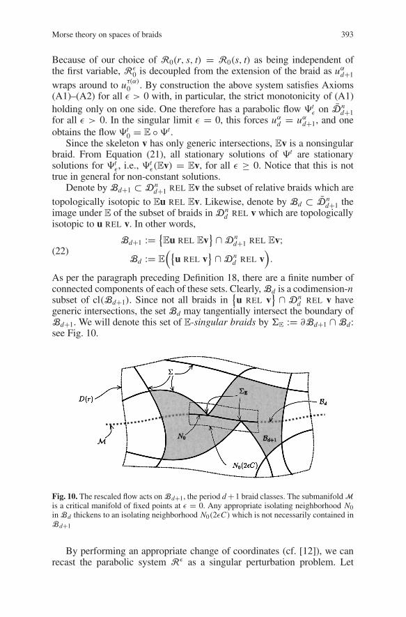
generic intersections, the set Bd may tangentially intersect the boundary ofBd+1. We will denote this set of E-singular braids by ΣE := ∂Bd+1 ∩Bd:see Fig. 10.
Fig. 10. The rescaled flow acts on Bd+1, the period d+1 braid classes. The submanifold Mis a critical manifold of fixed points at ε = 0. Any appropriate isolating neighborhood N0in Bd thickens to an isolating neighborhood N0(2εC) which is not necessarily contained inBd+1
By performing an appropriate change of coordinates (cf. [12]), we canrecast the parabolic system Rε as a singular perturbation problem. Let

394 R.W. Ghrist et al.
x = (x j)ndj=1, with xi+1+(α−1)d := uα
i , and let y = (yα)nα=1, with yα :=
(uαd+1 − uα
d). Upon rescaling time as τ := t/ε, the vector field induced byour choice of Rε is of the form
dxdτ
= εX(x, y),
dydτ= −y+ εY(x),
(23)
for some (unspecified) vector fields X and Y with the functional dependenceindicated. The product flow of this vector field (23) in the new coordinatesis denoted by Φτ
ε and is well-defined on Dnd+1. In the case ε = 0, the set
M := y = 0 ⊂ Dnd+1 is a submanifold of fixed points containing Bd for
which the flow Φτ0 is transversally nondegenerate (since here y′ = −y). By
construction cl(Bd) = cl(Bd+1)∩M, as illustrated in Fig. 10 (in the simplecase where all braid classes are free and Bd+1 is thus connected).
The remainder of the analysis is a technique in singular perturbationtheory following [12]: one relates the τ-dynamics of Equation (23) to thoseof the t-dynamics on M, whose orbits are of the form (x(t), 0), where x(t)satisfies the limiting equation dx/dt = X(x, 0). The Conley index theory iswell-suited to this situation.
For any compact set D ⊂M and r ∈ R, let D(r) := (x, y) | (x, 0) ∈ D,
‖y‖ ≤ r denote the “product” radius r neighborhood in Dnd+1. Denote by
C = C(D) the maximal value C := maxD ‖Y(x)‖. Due to the specific formof (23), we obtain the following uniform squeezing lemma.
Lemma 21. If S is any invariant set of Φτε contained in some D(r), then in
fact S ⊂ D(εC). Moreover, for all points (x, y) with x ∈ D and ‖y‖ = 2εCit holds that d
dτ‖y‖ < 0.
Proof. Let (x, y)(τ) be an orbit in S contained in some D(r). Take the innerproduct of the y-equation with y:⟨
dydτ
, y⟩(τ0) = −‖y(τ0)‖2 + ε〈Y(x(τ0)), y(τ0)〉,
≤ −‖y‖2 + εC‖y‖.Hence d
dτ‖y‖ ≤ −‖y‖+εC, and we conclude that if ‖y(τ0)‖ > εC for some
τ0 ∈ R, then ddτ‖y‖ < 0. Consequently ‖y(τ)‖ grows unbounded for τ < τ0
and therefore (x, y) ∈ S, a contradiction. Thus ‖y(τ)‖ ≤ εC for all τ ∈ R.For points (x, y) with x ∈ D and ‖y‖ = 2εC, the above inequality gives
that ddτ‖y‖ ≤ −‖y‖ + εC < 0.
By compactness of the proper braid class, it is clear that Bd+1, and thusthe maximal isolated invariant set of Φτ
ε given by Sε := INV(Bd+1,Φτε )
8, isstrictly contained (and thus isolated) in D(r) for some compact D ⊂M and
8 Since Bd+1 is a proper braid class Sε is contained in its interior.

Morse theory on spaces of braids 395
some r sufficiently large. Fix C := C(D) as above. Lemma 21 now impliesthat as ε becomes small, Sε is squeezed into D(εC) – a small neighborhoodof a compact subset D of the critical manifold M, as in Fig. 10.9
This proximity of Sε to M allows one to compare the dynamics of theε = 0 and ε > 0 flows. Let N0 ⊂ Bd ⊂ M be an isolating neighborhood(isolating block with corners) for the maximal t-dynamics invariant setS0 := INV(Bd,Ψ
t0) within the braid class Bd. Combining Lemma 21 above,
Theorem 2.3C of [12], and the existence theorems for isolating blocks [60],one concludes that if (N0, N−0 ) is an index pair for the limiting equationsdx/dt = X(x, 0) then N0(2εC) is an isolating block for Φt
ε for 0 < ε ≤ε∗(N0) with ε∗ sufficiently small. A suitable index pair for the flow Φτ
ε ofEquation (23) is thus given by(
N0(2εC), N−0 (2εC)).(24)
Clearly, then, the homotopy index of S0 is equal to the homotopy indexof INV(N0(2εC)) for all ε sufficiently small. It remains to show that thiscaptures the maximal invariant set Sε.
Lemma 22. For all sufficiently small ε, INV(N0(2εC),Φτε ) = Sε.
Proof. By the choice of D it holds that Sε ⊂ D(2εC). We start by provingthat Sε ⊂ N0(2εC) for ε sufficiently small. Assume by contradiction thatSε j ⊂ N0(2ε jC) for some sequence ε j → 0. Then, since N0(2εC) isan isolating neighborhood for ε ≤ ε∗, there exist orbits (xε j , yε j ) in Sε j
such that (xε j , yε j )(τ j) ∈ D(2ε jC) − N0(2ε jC), for some τ j ∈ R. Define(xε j , yε j )(τ) = (xε j , yε j )(τ − τ j), and set (aε j , bε j )(t) = (xε j , yε j )(τ). Thesequence (aε j , bε j ) satisfies the equations
d
dtaε j = X(aε j , bε j ),
d
dtbε j = −
1
εbε j + Y(aε j ).(25)
By assumption ‖bε j (t)‖ ≤ Cε j , and ‖aε j‖, ‖daε j /dt‖ ≤ C, for all t ∈ Rand all ε j . An Arzela-Ascoli argument then yields the existence of an orbit(a∗(t), 0) ⊂ Bd, with (a∗(0), 0) ∈ cl(Bd − N0), satisfying the equationda∗dt = X(a∗, 0). By definition, (a∗, 0) ∈ INV(Bd) = INV(N0) ⊂ int(N0),
a contradiction, which proves that Sε ⊂ N0(2εC) for ε sufficiently small.The boundary of N0(2εC) splits as b1 ∪ b2, with
b1 = (x, y) | ‖y‖ = 2εC, and b2 = (x, y) | x ∈ ∂N0.Since the compact set N0 is contained in Bd, the boundary component b2is contained in Bd+1 provided that ε is sufficiently small. If the set ΣEis non-empty then the boundary component b1 never lies entirely in Bd+1regardless of ε. As ε → 0 the set N0(2εC)−(
Bd+1∩N0(2εC))
is contained
9 If one applies singular perturbation theory it is possible to construct an invariant manifoldMε ⊂ D(εC). The manifold Mε lies strictly within Bd+1 and intersects M at rest points ofthe Φt
0.

396 R.W. Ghrist et al.
is arbitrary small neighborhood of ΣE. Independent of the parabolic flow inquestion, and thus of ε, there exists a neighborhood K ⊂ Σn
d+1 REL v of ΣEon which the co-orientation of the boundary is pointed inside the braid classBd+1. In other words for every parabolic system the points in K enter Bd+1
under the flow, see Fig. 11. By using coordinates uαi − uα′
i and uαi+1 − uα′
i+1
ui+1α ui+1
α_
uα uα_i i
Fig. 11. The local picture of a generic singular tangency between strands α (solid) and α′(dashed). The shaded region represents Bd+1
adapted to the singular strands, it it easily seen (Fig. 11) that the braids aresimplified by moving into the set Bd+1.
We now show that INV(N0(2εC)) ⊂ Bd+1∩ N0(2εC). If not, then thereexist points (xε j , yε j ) ∈
[N0(2ε jC)−(
Bd+1∩N0(2ε jC))]∩INV(N0(2ε jC))
for some sequence ε j → 0. Consider the α-limit sets αε j ((xε j , yε j )). Since(xε j , yε j ) ∈ INV(N0(2ε jC)), and since Φτ
ε j((xε j , yε j )) cannot enter Bd+1 ∩
N0(2ε jC) in backward time due to the co-orientation of K , it follows thatαε j ((xε j , yε j )) is contained in N0(2ε jC)− (
Bd+1 ∩ N0(2ε jC)).
By a similar Arzela-Ascoli argument as before, this yields a set α0 ⊂ ΣEwhich is invariant for the flow Ψt
0. However due to the form of the vectorfield the associated flow Ψt
0 cannot contain an invariant set in ΣE, whichproves that INV(N0(2εC)) ⊂ Bd+1 ∩ N0(2εC) for ε sufficiently small.
Finally, knowing that Sε ⊂ INV(N0(2εC)), and that for sufficientlysmall ε it holds INV(N0(2εC) = INV(Bd+1 ∩ N0(2εC)) = Sε, it followsthat Sε = INV(N0(2εC)), which proves the lemma.
Theorem 20 now follows. Since, by Theorem 15, the homotopy indexis independent of the parabolic flow used to compute it, one may choosethe parabolic flow Φτ
ε for ε > 0 sufficiently small. The homotopy index ofΦτ
ε on the maximal invariant set Sε yields the wedge of all the connectedcomponents: H(Eu REL Ev). We have computed that this index is equal tothe index of Ψt on the original braid class: H(u REL v).

Morse theory on spaces of braids 397
Remark 23. The proof of Theorem 20 implies that any component of theperiod-(d+1) braid class Bd+1 which does not intersect M must necessarilyhave trivial index.
Remark 24. The above procedure also yields a stabilization result forbounded proper classes which are not bounded as topological classes. Inthis case one simply augments the skeleton v by two constant strands asfollows. Define the augmented braid v∗ := v ∪ v− ∪ v+, where
v−i := minα,i
vαi − 1, v+i := max
α,ivα
i + 1.(26)
Suppose [u REL v] ⊂ Dnd0
REL v is bounded for some period d0. It nowholds that h(u REL v) = h(u REL v∗), and
u REL v∗ is a bounded class.
It therefore follows from Theorem 19 thatmd0∨j=0
h(u( j) REL v
) = H(u REL v∗),(27)
where H can be evaluated via any discrete representative ofu REL v∗
of any admissible period.
5.3. Eventually free classes. At the end of this subsection, we completethe proof of Theorem 19. The preliminary step is to show that discretizedbraid classes are eventually free under E.
Given a braid u ∈ Dnd , consider the extension Eu of period d+1. Assume
at first the simple case in which d = 1, so that Eu is a period-2 braid. Drawthe braid diagram β(Eu) as defined in Sect. 2 in the domain [0, 2] × R.Choose any 1-parameter family of curves γs : t → ( fs(t), t) ∈ (0, 2) × Rsuch that γ0 : t → (1, t) and so that γs is transverse10 to the braid diagramβ(Eu) for all s. Define the braid γs · Eu as follows:
(γs · Eu)αi :=
(Eu)α
i : i = 0, 2
γs ∩ (Eu)α : i = 1.(28)
The point γs ∩ (Eu)α is well-defined since γs is always transverse to thebraid strands and γ0 intersects each strand but once.
Lemma 25. For any such family of curves γs, [γs · Eu] = [Eu].Proof. It suffices to show that this path of braids does not intersect thesingular braids Σ. Since u is assumed to be a nonsingular braid, everycrossing of two strands in the braid diagram of Eu is a transversal crossingbetween i = 0 and i = 1. Thus, if for some s, γs(t)∩ (Eu)α = γs(t)∩ (Eu)α′
for distinct strands α and α′, then(Euα
0 − Euα′0
) (Euα
1 − Euα′1
)< 0.(29)
10 At the anchor points, the transversality should be topological as opposed to smooth.

398 R.W. Ghrist et al.
The braid γs · Eu has a crossing of the α and α′ strands at i = 1. Checkingthe transversality of this crossing yields(
(γs · Eu)α0 − (γs · Eu)α′
0
) ((γs · Eu)α
2 − (γs · Eu)α′2
)=
((Eu)α
0 − (Eu)α′0
)((Eu)α
2 − (Eu)α′2
)=
((Eu)α
0 − (Eu)α′0
)((Eu)α
1 − (Eu)α′1
)< 0.
(30)
Thus the crossing is transverse and the braid is never singular. Note that the proof of Lemma 25 does not require the braid Eu to be
a closed braid diagram since the isotopy fixes the endpoints: the proof isequally valid for any localized region of a braid in which one spatial segmenthas crossings and the next segment has flat strands.
Corollary 26. The “shifted” extension operator which inserts a trivialperiod-1 braid at the ith discretization point in a braid has the same actionon components of Dd as does E.
Fig. 12. Relations in the braid group via discrete isotopy
Proposition 27. The period-d discretized braid class [u] is free whend > |u|word.
Proof. We must show that any braid u′ ∈ Dnd which has the same topological
type as u is discretely isotopic to u. Place both u and u′ in general position soas to record the sequences of crossings using the generators of the n-strandpositive braid semigroup, σi, as in Sect. 2. Recall the braid group hasrelations σiσ j = σ jσi for |i − j| > 1 and σiσi+1σi = σi+1σiσi+1; closurerequires making conjugacy classes equivalent.
The conjugacy relation can be realized by a discrete isotopy as follows:since d > |u|word, u must possess some discretization interval on whichthere are no crossings. Lemma 25 then implies that this interval withoutcrossings commutes with all neighboring discretization intervals via discreteisotopies. Performing d consecutive exchanges shifts the entire braid overby one discretization interval. This generates the conjugacy relation.

Morse theory on spaces of braids 399
To realize the remaining braid relations in a discrete isotopy, assumefirst that u and u′ are of the form that there is at most one crossing perdiscretization interval. It is then easy to see from Fig. 12 that the braidrelations can be executed via discrete isotopy.
In the case where u (and/or u′) exhibits multiple crossings on somediscretization intervals, it must be the case that a corresponding numberof other discretization intervals do not possess any crossings (since d >|u|word). Again, by inductively utilizing Lemma 25, we may redistributethe intervals-without-crossing and “comb” out the multiple crossings viadiscrete isotopies so as to have at most one crossing per discretizationinterval. Proof of Theorem 19. Assume that
u REL v =
u′ REL v′. Thisimplies that there is a path of topological braid diagrams taking the pair(u, v) to (u′, v′). This path may be chosen so as to follow a sequence ofstandard relations for closed braids. From the proof of Proposition 27, theserelations may be performed by a discretized isotopy to connect the pair(E ju,E jv) to (Eku′,Ekv′) for j and k sufficiently large, and of the rightrelative size to make the periods of both pairs equal. For this choice, then,[E
ju REL [E jv]] = [E
ku′ REL [Ekv′]], and their homotopy indices agree.An application of Theorem 20 completes the proof.
We suspect that all braids in the image of E are free: a result which, iftrue, would simplify index computations yet further.
6. Duality
For purposes of computation of the index, we will often pass to the homo-logical level. In this setting, there is a natural duality made possible by thefact that the index pair used to compute the index of a braid class can bechosen to be a manifold pair.
Definition 28. The duality operator on discretized braids is the map D :Dn
2p → Dn2p given by
(Du)αi := (−1)iuα
i .(31)
Clearly D induces a map on relative braid diagrams by definingD(u REL v) to be Du REL Dv. The topological action of D is to inserta half-twist at each spatial segment of the braid. This has the effect oflinking unlinked strands, and, since D is an involution, linked strands areunlinked by D: see Fig. 13.
For the duality statements to follow, we assume that all braids consideredhave even periods and that all of the braid classes and their duals are proper,so that the homotopy index is well-defined.

400 R.W. Ghrist et al.
Fig. 13. The topological action of D
Lemma 29. The duality map D respects braid classes: if [u] = [u′] then[D(u)] = [D(u′)]. Bounded braid classes are taken to bounded braid classesby D.
Proof. It suffices to show that the map D is a homeomorphism on the pair(Dn
2p,Σ). This is true on Dn2p since D is a smooth involution (D−1 = D). If
u ∈ Σ with uαi = uα′
i and(uα
i−1 − uα′i−1
)(uα
i+1 − uα′i+1
) ≥ 0,(32)
then applying the operator D yields points Duαi = Duα′
i with each term inthe above inequality multiplied by−1 (if i is even) or by+1 (if i is odd): ineither case, the quantity is still non-negative and thusDu ∈ Σ. Boundednessis clearly preserved. Theorem 30. (a) The effect ofD on the index pair is to reverse the direction
of the parabolic flow.(b) For [u REL v] ⊂ Dn
2p REL v of period 2p with n free strands,
CH∗(h(D(u REL v));R) ∼= CH2n p−∗(h(u REL v);R).(33)
(c) For [u REL v] ⊂ Dn2p REL v of period 2p with n free strands,
CH∗(H(D(u REL v));R) ∼= CH2n p−∗(H(u REL v);R).(34)
Proof. For (a), let (N, N−) denote an index pair associated to a properrelative braid class [u REL v]. Dualizing sends N to a homeomorphic spaceD(N). The following local argument shows that the exit set of the dualbraid class is in fact the complement (in the boundary) of the exit set of thedomain braid: specifically,
(D(N))− = cl∂(D(N))− D(N−)
.
Let w ∈ [u REL v] ∩ Σ. At any singular anchor point of w, i.e., wherewα
i = wα′i and the transversality condition is not satisfied, then it follows
from Axiom (A2) that
SIGN
d
dt
(wα
i −wα′i
) = SIGNwα
i−1 −wα′i−1
.(35)

Morse theory on spaces of braids 401
(Depending on the form of (A2) employed, one might use wαi+1 − wα′
i+1 onthe right hand side without loss.) Since the subscripts on the left side havethe opposite parity of the subscripts on the right side, taking the dual braid(which multiplies the anchor points by (−1)i and (−1)i−1 respectively)alters the sign of the terms. Thus, the operator D reverses the direction ofthe parabolic flow.
From this, we may compute the Conley index of the dual braid byreversing the time-orientation of the flow. Since one can choose the indexpair used to compute the index to be an oriented manifold pair (specifically,an isolating block: see, e.g., [60]), one may then apply a Poincare-Lefschetzduality argument as in [44] and use the fact that the dimension is 2np toobtain the duality formula for homology. This yields (b).
The final claim (c) follows from (b) by showing that D is bijective ontopological braid classes within Dn
2p. Assume that [u REL v] and [u′ REL v]are distinct braid classes in Dn
2p of the same topological type. Since D isa homeomorphism on Dn
2p, the dual classes [Du REL Dv] and [Du′ REL Dv]are distinct. Claim (c) follows upon showing that these duals are still topo-logically the same braid class.
Proposition 27 implies that [(E2ku) REL (E2kv)] = [(E2ku′) REL (E2kv)]for k sufficiently large since u REL v = u′ REL v. By Lemma 29,
D[(E2ku) REL (E2kv)
] = D [(E2ku′) REL (E2kv)
],
which, by Lemma 7 means that these braids are topologically the same. Thetopological action of dualizing the 2k-stabilizations of u REL v and u′ REL vis to add k full twists. Since the full twist is in the center of the braid group(this element commutes with all other elements of the braid group [8]), onecan factor the dual braids within the topological braid group and mod outby k full twists, yielding that Du REL Dv =
Du′ REL Dv.
We use this homological duality to complete a crucial computation inthe proof of the forcing theorems (e.g., Theorem 1) at the end of thispaper. The following small corollary uses duality to give the first steptowards answering the question of just what the homotopy index measurestopologically about a braid class. Recall the definition of an augmentedbraid from Remark 24.
Corollary 31. Consider the dual of any augmented proper relative braid.Adding a full twist to this dual braid shifts the homology of the index up bytwo dimensions.
Proof. Assume that D[u REL v∗] is the dual of an augmented braid inperiod 2p (the augmentation is required to keep the braid class boundedupon adding a full twist). The prior augmentation implies that the outertwo strands of Dv “maximally link” the remainder of the relative braid. Theeffect of adding a full twist to this braid can be realized by instead stabilizing

402 R.W. Ghrist et al.
[u REL v∗] twice and then dualizing. The homological duality implies thatfor each connected component of the topological class,
CH∗(h(DE2(u REL v∗))) ∼= CH2n p+2−∗(h(E2(u REL v∗)))∼= CH2n p+2−∗(h(u REL v∗))∼= CH∗−2(h(D(u REL v∗))),
(36)
which gives the desired result for the index H via Theorem 30. Remark 32. The homotopy version of (36) can be achieved by followinga similar procedure as in Sect. 5. One obtains a double-suspension of thehomotopy index, as opposed to a shift in homology.
Remark 33. Given a braid class [u] of odd period p = 2d + 1, the imageunder D is not necessarily a discretized braid at all: without some symmetrycondition, the braid will not “close up” at the ends. To circumvent this,define the dual of u to be the braid D(u2) – the dual of the period 2pextension of u. The analogue of Theorem 30 above is that
CH∗(H(SYM(D(u RELv)));R) ∼= CHn p−∗(H(u REL v);R),(37)
where SYM denotes the subset of the braid class which consists of symmetricbraids: uα
i = uα2p−i for all i.
7. Morse theory
It is clear that the Morse-theoretic content of the homotopy index on braidsholds implications for the dynamics of parabolic flows and thus zeros ofparabolic recurrence relations. With this in mind, we restrict ourselves tobounded proper braid classes.
Recall that the characteristic polynomial of an index pair (N, N−) is thepolynomial
CPt(N) :=∑k≥0
βktk;
βk(N) := dimCHk(N;R) = dim Hk(N, N−;R).
(38)
The Morse relations in the setting of the Conley index (see [14]) state that ifN has a Morse decomposition into distinct isolating subsets NaCa=1, then
C∑a=1
CPt(Na) = CPt(N) + (1+ t)Qt,(39)
for some polynomial Qt with nonnegative integer coefficients.

Morse theory on spaces of braids 403
7.1. The exact, nondegenerate case. For parabolic recurrence relationswhich satisfy (A3) (gradient type) it holds that if h(u REL v) = 0, then Rhas at least one fixed point in [u REL v]. Indeed, one has:
Lemma 34. For an exact nondegenerate parabolic flow on a boundedproper relative braid class, the sum of the Betti numbers βk of h, as de-fined in (38), is a lower bound on the number of fixed points of the flow onthat braid class.
Proof. The details of this standard Morse theory argument are provided forthe sake of completeness. Choose Ψt a nondegenerate gradient parabolicflow on [u REL v] (in particular, Ψt fixes v for all time). Enumerate the[finite number of] fixed points uaCa=1 of Ψt on this [bounded] braid class. Bynondegeneracy, the fixed point set may be taken to be a Morse decompositionof INV(N). The characteristic polynomial of each fixed point is merelytµ∗(ua), where µ∗(ua) is the Morse co-index of ua. Substituting t = 1 into
Equation (39) yields the lower bound
#Fix([u REL v],Ψt) ≥∑
k
βk(h).(40)
On the level of the topological braid invariant H, one needs to sum
over all the path components as follows. As in Theorem 19, choose period-d representatives u( j) ( j from 0 to m) for each path component of thetopological class
u REL v. If we consider fixed points in the union
∪mj=0[u( j) REL v], we obtain the following Morse inequalities from (40)
and Theorem 19:
#Fix(∪mj=0[u( j) REL v],Ψt) ≥
∑k
βk(H),(41)
where βk(H) is the kth Betti number of H(u REL v∗). Thus, again, the sum ofthe Betti numbers is a lower bound, with the proviso that some componentsmay not contain any critical points.
If the topological classu REL v is bounded the inequality (41) holds
with the invariant H(u REL v).
7.2. The exact, degenerate case. Here a coarse lower bound still exists.
Lemma 35. For an arbitrary exact parabolic flow on a bounded relativebraid class, the number of fixed points is bounded below by the number ofdistinct nonzero monomials in the characteristic polynomial CPt(h).
Proof. Assuming that #Fix is finite, all critical points are isolated and forma Morse decomposition of INV(N). The specific nature of parabolic recur-rence relations reveals that the dimension of the null space of the linearizedmatrix at an isolated critical point is at most 2, see e.g. [56]. Using this factDancer proves [15], via the degenerate version of the Morse lemma due

404 R.W. Ghrist et al.
to Gromoll and Meyer, that CHk(ua) = 0 for at most one index k = k0.Equation (39) implies that,
Cd∑a=1
CPt(ua) ≥ CPt(h)(42)
on the level of polynomials. As the result of Dancer implies that foreach a, CPt(ua) = Atk , for some A ≥ 0, it follows that the number ofcritical points needs to be at least the number of non-trivial monomialsin CPt(h).
As before, if we instead use the topological invariant H foru REL v∗
we obtain that the number of monomials in CPt(H) is a lower bound for thetotal sum of fixed points over the topologically equivalent path-components.
More elaborate estimates in some cases can be obtained via the extensionof the Conley index due to Floer [17].
7.3. The non-exact case. If we consider parabolic recurrence relations thatare not necessarily exact, the homotopy index may still provide informationabout solutions of R = 0. This is more delicate because of the possibilityof periodic solutions for the flow u′i = Ri(ui−1, ui, ui+1). For example, ifCPt(h) mod (1+ t) = 0, the index does not provide information about ad-ditional solutions for R = 0, as a simple counterexample shows. However,if CPt(h) mod (1+ t) = 0, then there exists at least one solution of R = 0with the specified relative braid class. Specifically,
Lemma 36. An arbitrary parabolic flow on a bounded relative braid classis forced to have a fixed point if χ(h) := CP−1(h) is nonzero. If the flowis nondegenerate, then the number of fixed points is bounded below by thequantity (
CPt(h) modZ+[t] (1+ t))∣∣
t=1 .(43)
Proof. Set N = cl([u REL v]). As the vector field R has no zeros at ∂N, theBrouwer degree, deg(R, N, 0), may be computed via a small perturbationR and is given by11
deg(R, N, 0) :=∑
u∈N,R(u)=0
sign det(−dR(u)).
For a generic perturbation R the associated parabolic flow Ψt is a Morse-Smale flow [21]. The (finite) collection of rest points ua and periodicorbits γb of Ψt then yields a Morse decomposition of Inv(N), and theMorse inequalities are∑
a
CPt(ua)+∑
b
CPt(γb) = CPt(h)+ (1+ t)Qt .
11 We choose to define the degree via −dR in order to simplify the formulae.

Morse theory on spaces of braids 405
The indices of the fixed points are given by CPt(ua) = tµ∗(ua), where µ∗ is
the number of eigenvalues of dR(ua) with positive real part, and the indicesof periodic orbits are given by CPt(γb) = (1+ t)tµ
∗(γb). Upon substitutionof t = −1 we obtain
deg(R, N, 0) = deg(R, N, 0) =∑
a
(−1)µ∗(ua)
=∑
a
CP−1(ua) = CP−1(h) = χ(h).
Thus, if the Euler characteristic of h is non-trivial, then R has at least onezero in N.
In the generic case the Morse relations give even more information.One has CPt(h) = p1(t) + (1 + t)p2(t), with p1, p2 ∈ Z+[t], andCPt(h) modZ+[t] (1 + t) = p1(t). It then follows that
∑a CPt(ua) ≥
CPt(h) modZ+[t] (1+ t), proving the stated lower bound. The obvious extension of these results to the full index H is left to the
reader.
8. Second order Lagrangian systems
In this final third of the paper, we apply the developed machinery to theproblem of forcing closed characteristics in second order Lagrangian sys-tems of twist type. The vast literature on fourth order differential equationscoming from second order Lagrangians includes many physical models innonlinear elasticity, nonlinear optics, physics of solids, Ginzburg-Landauequations, etc. (see Sect. 1). In this context we mention the work of [1,38,49,50].
8.1. Twist systems. We recall from Sect. 1 that closed characteristics atan energy level E are concatenations of monotone laps between minimaand maxima (ui)i∈Z, which are periodic sequences with even period 2p.The extrema are restricted to the set UE , whose connected components aredenoted by IE : interval components (see Sect. 1.2 for the precise definition).The problem of finding closed characteristics can, in most cases, be formu-lated as a finite dimensional variational problem on the extrema (ui). Thefollowing twist hypothesis, introduced in [58], is key:
(T): infJE[u] =∫ τ
0
(L(u, ux, uxx)+ E
)dx | u ∈ Xτ (u1, u2), τ ∈ R+ has
a minimizer u(x; u1, u2) for all (u1, u2) ∈ IE × IE | u1 = u2, and uand τ are C1-smooth functions of (u1, u2).
Here Xτ = Xτ (u1, u2) = u ∈ C2([0, τ]) | u(0) = u1, u(τ) = u2, ux(0) =ux(τ) = 0 and ux |(0,τ) > 0.
Hypothesis (T) is a weaker version of the hypothesis that assumes thatthe monotone laps between extrema are unique (see, e.g., [34,35,58]). Hy-pothesis (T) is valid for large classes of Lagrangians L . For example, if

406 R.W. Ghrist et al.
L(u, v,w) = 12w
2 + K(u, v), the following two inequalities ensure thevalidity of (T):
(a) ∂K∂v
v − K(u, v)− E ≤ 0, and
(b) ∂2 K∂v2 |v|2 − 5
2
∂K∂v
v− K(u, v)− E ≥ 0 for all u ∈ IE and v ∈ R.
Many physical models, such as the Swift-Hohenberg equation (3), meetthese requirements, although these conditions are not always met. In thosecases numerical calculations still predict the validity of (T), which leavesthe impression that the results obtained for twist systems carry over tomany more systems for which Hypothesis (T) is hard to check.12 For thesereasons twist systems play a important role in understanding second orderLagrangian systems. For a direct application of this see [31].
The existence of minimizing laps is valid under very mild hypotheseson K (see [31]). In that case (b) above is enough to guarantee the validity of(T). An example of a Lagrangian that satisfies (T), but not (a) is given by theErickson beam-model [30,49,55] L(u, ux, uxx) = α
2 |uxx |2 + 14 (|ux|2 − 1)2
+ β
2 u2.
8.2. Discretization of the variational principle. We commence by re-peating the underlying variational principle for obtaining closed character-istics as described in [58]. In the present context a broken geodesic is aC2-concatenation of monotone laps (alternating between increasing and de-creasing laps) given by Hypothesis (T). A closed characteristic u at energylevel E is a (C2-smooth) function u : [0, τ] → R, 0 < τ < ∞, which isstationary for the action JE[u] with respect to variations δu ∈ C2
per(0, τ),and δτ ∈ R+, and as such is a ‘smooth broken geodesic’.
The following result, a translation of results implicit in [58], is themotivation and basis for the applications of the machinery in the first two-thirds of this paper.
Theorem 37. Extremal points ui for bounded solutions of second orderLagrangian twist systems are solutions of an exact parabolic recurrencerelation with the constraints that (i) (−1)iui < (−1)iui+1; and (ii) therecurrence relation blows up along any sequence satisfying ui = ui+1.
Proof. For simplicity, we restrict to the case of a nonsingular energy level E:for singular energy levels, a slightly more involved argument is required. De-note by I the interior of IE , and by ∆(I ) = ∆ := (u1, u2) ∈ I×I | u1 = u2the diagonal. Then define the generating function
S : (I × I ) \∆→ R ; S(u1, u2) :=∫ τ
0
(L(u, ux, uxx)+ E
)dx;(44)
12 Another method to implement the ideas used in this paper is to set up a curve-shorteningflow for second order Lagrangian systems in the (u, u′) plane.

Morse theory on spaces of braids 407
the action of the minimizing lap from u1 to u2. That S is a well-definedfunction is the content of Hypothesis (T). The action functional associatedto S for a period 2p system is the function
W2p(u) :=2p−1∑i=0
S(ui, ui+1).
Several properties of S follow from [58]:
(a) [smoothness] S ∈ C2(I × I\∆).(b) [monotonicity] ∂1∂2S(u1, u2) > 0 for all u1 = u2 ∈ I .(c) [diagonal singularity] lim
u1u2−∂1S(u1, u2) = lim
u2u1∂2S(u1, u2) =
limu1u2
∂1S(u1, u2) = limu2u1
−∂2S(u1, u2) = +∞.
In general the function ∂1S(u1, u2) is strictly increasing in u2 for all u1 ≤u2 ∈ IE , and similarly ∂2S(u1, u2) is strictly increasing in u1. The functionS also has the additional property that S|∆ ≡ 0.
Critical points of W2p satisfy the exact recurrence relation
Ri(ui−1, ui, ui+1) := ∂2S(ui−1, ui)+ ∂1S(ui, ui+1) = 0,(45)
where Ri(r, s, t) is both well-defined and C1 on the domains
Ωi = (r, s, t) ∈ I 3 | (−1)i+1(s − r) > 0, (−1)i+1(s − t) > 0,by Property (a). The recurrence function R is periodic with d = 2, as arethe domains Ωi .13 Property (b) implies that Axiom (A1) is satisfied. Indeed,∂1Ri = ∂1∂2S(ui−1, ui) > 0, and ∂3Ri = ∂1∂2S(ui, ui+1) > 0.
Property (c) provides information about the behavior of R at the diagonalboundaries of Ωi , namely,
limsr Ri(r, s, t) = limst Ri(r, s, t) = +∞limsr Ri(r, s, t) = limst Ri(r, s, t) = −∞(46)
The parabolic recurrence relations generated by second order Lagrang-
ians are defined on the constrained polygonal domains Ωi .
Definition 38. A parabolic recurrence relation is said to be of up-downtype if (46) is satisfied.
In the next subsection we demonstrate that the up-down recurrence rela-tions can be embedded into the standard theory as developed in Sects. 2–7.
8.3. Up-down restriction. The variational set-up for second order La-grangians introduces a few complications into the scheme of parabolicrecurrence relations as discussed in Sects. 2–7. The problem of boundary
13 We could also work with sequences u that satisfy (−1)i+1(ui+1 − ui) > 0.

408 R.W. Ghrist et al.
conditions will be considered in the following section. Here, we retool themachinery to deal with the fact that maxima and minima are forced toalternate. Such braids we call up-down braids.14
8.3.1. The space E .
Definition 39. The spaces of general/nonsingular/singular up-down braiddiagrams are defined respectively as:
En2p := Dn
2p ∩u : (−1)i
(uα
i+1 − uαi
)> 0 ∀i, α
,
En2p := Dn
2p ∩u : (−1)i
(uα
i+1 − uαi
)> 0 ∀i, α
,
ΣE := En2p − En
2p.
Path components of En2p comprise the up-down braid types [u]E , and path
components in En2p REL v comprise the relative up-down braid types
[u REL v]E .
The set En2p has a boundary in Dn
2p
∂En2p = ∂
(Dn
2p ∩u : (−1)i
(uα
i+1 − uαi
) ≥ 0 ∀i, α)
.(47)
Such braids, called horizontal singularities, are not included in the definitionof En
2p since the recurrence relation (45) does not induce a well-defined flow
on the boundary ∂En2p.
Lemma 40. For any parabolic flow of up-down type on En2p, the flow blows
up in a neighborhood of ∂En2p in such a manner that the vector field points
into En2p. All of the conclusions of Theorem 15 hold upon considering the
ε-closure of braid classes [u REL v]E in En2p, denoted
clE ,ε[u REL v]E:=
u REL v ∈ clE [u REL v]E : (−1)i
(uα
i+1 − uαi
) ≥ ε ∀i, α,
for all ε > 0 sufficiently small.
Proof. The proof that any parabolic flow Ψt of up-down type acts here soas to strictly decrease the word metric at singular braids is the same proofas used in Proposition 11. The only difficulty arises in what happens at theboundary of En
2p: we must show that Ψt respects the up-down restriction inforward time.
Define the function
ε(u) = mini,α
∣∣uαi − uα
i+1
∣∣.14 The more natural term alternating has an entirely different meaning in knot theory.

Morse theory on spaces of braids 409
Clearly, if ε(u) = 0, then u ∈ ∂En2p. Let u ∈ En
2p, and consider the evo-lution Ψt(u), t > 0. We compute d
dt ε(Ψt(u)) as ε(Ψt(u)) becomes small.
Using (45) it follows that
d
dt
(uα
i − uαi+1
) = Ri(uα
i−1, uαi , uα
i+1
)−Ri+1(uα
i , uαi+1, uα
i+2
)→∞,
as ui ui+1, (i odd),
d
dt
(uα
i+1 − uαi
) = Ri+1(uα
i , uαi+1, uα
i+2
)−Ri(uα
i−1, uαi , uα
i+1
)→∞,
as ui ui+1, (i even).
These inequalities show that ddt ε(Ψ
t(u)) > 0 as soon as ε(Ψt(u)) becomestoo small. Due to the boundedness of [u REL v]E and the infinite repulsionat ∂En
2p, we can choose a uniform ε(u REL v) > 0 so that ddt ε(Ψ
t(u)) > 0for ε(Ψt(u)) ≤ ε(u REL v), and thus clE,ε[u REL v]E is an isolating neigh-borhood for all 0 < ε ≤ ε(u REL v).
8.3.2. Universality for up-down braids. We now show that the topologicalinformation contained in up-down braid classes can be continued to thecanonical case described in Sect. 2. As always, we restrict attention toproper, bounded braid classes, proper being defined as in Definition 13, andbounded meaning that the set [u REL v]E is bounded in Dn
2p. Note that anup-down braid class [u REL v]E can sometimes be bounded while [u REL v]is not. To bounded proper up-down braids we assign a homotopy index.From Lemma 40 it follows that for ε sufficiently small the set NE,ε :=clE ,ε[u REL v]E is an isolating neighborhood in En
2p whose Conley index,
h(u REL v,E ) := h(NE,ε),
is well-defined with respect to any parabolic flow Ψt generated by a parabolicrecurrence relation of up-down type, and is independent of ε. As before, non-triviality of h(NE,ε) implies existence of a non-trivial invariant set insideNE,ε (see Sect. 8.3.3).
The obvious question is what relationship holds between the homotopyindex h(u REL v,E ) and that of a braid class without the up-down restriction.To answer this, augment the skeleton v as follows: define v∗ = v∪ v− ∪ v+,where
v−i := minα,i
vαi − 1+ (−1)i+1, v+i := max
α,ivα
i + 1+ (−1)i+1.
The topological braid class u REL v∗ is bounded and proper. Indeed,boundedness follows from adding the strands v± which bound u, sinceminα,i v
αi ≤ uα
i ≤ maxα,i vαi . Properness is satisfied since u REL v is
proper.

410 R.W. Ghrist et al.
Theorem 41. For any bounded proper up-down braid class [u REL v]E inEn
2p REL v,
h(u REL v,E ) = h(u REL v∗).
Proof. From Lemma 55 in Appendix A we obtain a parabolic recurrencerelation R0 (not necessarily up-down type) for which v∗ is a solution. Wedenote the associated parabolic flow by Ψt
0. Define two functions k1 and k2
in C1(R), with k′1 ≥ 0 ≥ k′2, and k1(τ) = 0 for τ ≤ −2δ, k1(−δ) ≥ K , andk2(τ) = 0 for τ ≥ 2δ, k2(δ) ≥ K , for some δ > 0 and K > 0 to be specifiedlater. Introduce a new recurrence function R1
i (r, s, t) = R0i (r, s, t)+k2(s−r)
+k1(t−s) for i odd, and R1i (r, s, t) = R0
i (r, s, t)−k1(s−r)−k2(t−s) for ieven. The associated parabolic flow will be denoted by Ψt
1, and Ψt1(v
∗) = v∗by construction by choosing δ sufficiently small. Indeed, if we chooseδ < ε(v), the augmented skeleton is a fixed point for Ψt
1.Since the braid class [u REL v∗] is bounded and proper, N1 = cl[u REL v∗]
is an isolating neighborhood with invariant set INV(N1). If we choose Klarge enough, and δ sufficiently small, then the invariant set INV(N1) liesentirely in clE,ε[u REL v∗]E = clE,ε[u REL v]E = NE,ε . Indeed, for large Kwe have that for each i, R1
i (r, s, t) has a fixed sign on the complement ofNE,ε . Therefore, h(u REL v∗) = h(N1) = h(NE,ε). Now restrict the flow Ψt
1
to NE,ε ⊂ En2p REL v. We may now construct a homotopy between Ψt
1 andΨt , via (1 − λ)R + λR1 (see Appendix A), where R and the associatedflow Ψt are defined by (45). The braid v∗ is stationary along the homotopyand therefore
h(N1) = h(NE,ε,Ψ
t1
) = h(NE,ε,Ψ
t),
which proves the theorem. We point out that similar results can be proved for other domains Ωi
with various boundary conditions. The key observation is that the up-downconstraint is really just an addition to the braid skeleton.
8.3.3. Morse theory. For bounded proper up-down braid classes [u REL v]Ethe Morse theory of Sect. 7 applies. Combining this with Lemma 40 andTheorem 41, the topological information is given by the invariant H of thetopological braid type
u REL v∗.
Corollary 42. On bounded proper up-down braid classes, the total numberof fixed points of an exact parabolic up-down recurrence relation is boundedbelow by the number of monomials in the critical polynomial CPt(H) of thehomotopy index.
Proof. Since all critical point are contained in NE,ε the corollary followsfrom the Lemmas 35, 40 and Theorem 41.

Morse theory on spaces of braids 411
9. Multiplicity of closed characteristics
We now have assembled the tools necessary to prove Theorem 1, the generalforcing theorem for closed characteristics in terms of braids, and Theorems 2and 3, the application to singular and near-singular energy levels. Givenone or more closed characteristics, we keep track of the braiding of theassociated strands, including at will any period-two shifts. Fixing thesestrands as a skeleton, we add hypothetical free strands and compute thehomotopy index. If nonzero, this index then forces the existence of the freestrand as an existing solution, which, when added to the skeleton, allowsone to iterate the argument with the goal of producing an infinite family offorced closed characteristics.
The following lemma (whose proof is straightforward and thus omitted)will be used repeatedly for proving existence of closed characteristics.
Lemma 43. Assume that R is a parabolic recurrence relation on Dnd with
u a solution. Then, for each integer N > 1, there exists a lifted parabolicrecurrence relation on Dn
Nd for which every lift of u is a solution. Further-more, any solution to the lifted dynamics on Dn
Nd projects to some period-dsolution.15
The primary difficulties in the proof of the forcing theorems are (i)computing the index (we will use all features of the machinery developedthus far, including stabilization and duality); and (ii) asymptotics/boundaryconditions related to the three types of closed interval components IE:a compact interval, the entire real line, and the semi-infinite ray.
All of the forcing theorems are couched in a little braid-theoretic lan-guage:
Definition 44. The intersection number of two strands uα, uα′ of a braid uis the number of crossings in the braid diagram, denoted
ι(uα, uα′) := # of crossings of strands.
The trivial braid on n strands is any braid (topological or discrete) whosebraid diagram has no crossings whatsoever, i.e., ι(uα, uα′) = 0, for allα, α′. The full-twist braid on n strands, is the braid of n connected compo-nents, each of which has exactly two crossings with every other strand, i.e.,ι(uα, uα′) = 2 for all α = α′.
Among discrete braids of period two, the trivial braid and the full twistare duals in the sense of Sect. 6.
9.1. Compact interval components. Let E be a regular energy level forwhich the set UE contains a compact interval component IE .
15 This does not imply a d-periodic solution, but merely a braid diagram u of period d.

412 R.W. Ghrist et al.
Theorem 45. Suppose that a twist system with compact IE possesses oneor more closed characteristics which, as a discrete braid diagram, forma nontrivial braid. Then there exists an infinity of non-simple, geometricallydistinct closed characteristics in IE.
In preparation for the proof of Theorem 45 we state a technical lemma,whose [short] proof may be found in [58].
Lemma 46. Let IE = [u−, u+], then there exists a δ0 > 0 such that
1. R1(u− + δ, u−, u− + δ) > 0, R1(u+, u+ − δ, u+) < 0, and2. R2(u−, u− + δ, u−) > 0, R2(u+ − δ, u+, u+ − δ) < 0,
for any 0 < δ ≤ δ0.
Proof of Theorem 45. Via Theorem 37, finding closed characteristics isequivalent to solving the recurrence relation given by (45). Define the do-mains
Ωδi =
(ui−1, ui, ui+1) ∈ I3
E
∣∣ u− + δ < ui±1 < ui − δ/2 < u+ − δ, i odd,
(ui−1, ui, ui+1) ∈ I3E
∣∣ u− + δ < ui + δ/2 < ui±1 < u+ − δ, i even,
For any integer p ≥ 1 denote by Ω2p the set of 2p-periodic sequences uifor which (ui−1, ui, ui+1) ∈ Ωδ
i . By Lemma 46, choosing 0 < δ < δ0 smallenough forces the vector field R = (Ri) to be everywhere transverse to∂Ω2p, making Ω2p positively invariant for the induced parabolic flow Ψt .
By Lemma 43, one can lift the assumed solution(s) to a pair of period2p single-stranded solutions to (45), v1 and v2, satisfying ι(v1, v2) = 0, forsome p ≥ 1. Define the cones
C− =u ∈ Ω2p
∣∣ ui ≤ vαi , α = 1, 2
, and
C+ =u ∈ Ω2p
∣∣ ui ≥ vαi , α = 1, 2
.
The combination of the facts ι(v1, v2) = r > 0, Axiom (A1), and thebehavior of R on ∂Ω2p implies that on the boundaries of the cones C−and C+ the vector field R is everywhere transverse and pointing inward.Therefore, C− and C+ are also positively invariant with respect to theparabolic flow Ψt . Consequently, W2p has global maxima v− and v+ onint(C−) and int(C+) respectively. The maxima v− and v+ have the propertythat v−i < vα
i < v+i , α = 1, 2. As a braid diagram, v = v1, v2, v−, v+ isa stationary skeleton for the induced parabolic flow Ψt .
Having found the solutions v− and v+ we now choose a compact intervalI IE , such that the skeletal strands are all contained in I . In this waywe obtain a proper parabolic flow (circumventing boundary singularities)which can be extended to a parabolic flow on E1
2p REL v. Let [u REL v]Ebe the relative braid class with a period 2p free strand u = ui which

Morse theory on spaces of braids 413
links the strands v1 and v2 with intersection number 2q while satisfyingv−i < ui < v+i : see Fig. 14 below.
-u
+v
v
v
1
v2
Fig. 14. A representative braid class for the compact case: q = 1, r = 4, 2p = 6
As an up-down braid class, [u REL v]E is a bounded proper braid classprovided 0 < 2q < r ≤ 2p, and the Morse theory discussed in Sect. 7 andSect. 8.3.3 then requires the evaluation of the invariant H of the topologicalclass
u REL v∗. In this case, since h(u REL v,E ) = h(u REL v∗) =
h(u REL v), augmentation is not needed, and H(u REL v∗) = H(u REL v).The nontriviality of the homotopy index H is given by the following lemma,whose proof we delay until Sect. 10.
Lemma 47. The Conley homology of H(u REL v) is given by:
CHk(H) =R : k = 2q − 1, 2q
0 : else.(48)
In particular CPt(H) = t2q−1(1+ t).
From the Morse theory of Corollary 42 we derive that for each q satisfying0 < 2q < r ≤ 2p there exist at least two distinct period-2p solutionsof (45), which generically are of index 2q and 2q − 1. In this manner, thenumber of solutions depends on r and p. To construct infinitely many, weconsider m-fold coverings of the skeleton v, i.e., one periodically extends vto a skeleton contained in E4
2pm , m ≥ 1. Now q must satisfy 0 < 2q < rm ≤2pm. By choosing triples (q, p, m) such that (q, pm) are relative prime,we obtain the same Conley homology as above, and therefore an infinity ofpairs of geometrically distinct solutions of (45), which, via Lemma 43 andTheorem 37 yield an infinity of closed characteristics.
Note that if we set qm = q and pm = pm, then the admissible ratios qmpm
for finding closed characteristics are determined by the relation
0 <qm
pm<
r
2p.(49)
Thus if v1 and v2 are maximally linked, i.e. r = 2p, then closed character-istics exist for all ratios in Q ∩ (0, 1).
414 R.W. Ghrist et al.
9.2. Non-compact interval components: IE = R. On non-compact inter-val components, closed characteristics need not exist. An easy example ofsuch a system is given by the quadratic Lagrangian L = 1
2 |uxx|2+ α2 |ux |2+
12 |u|2, with α > −2. Clearly IE = R for all E > 0, and the Lagrangiansystem has no closed characteristics for those energy levels. For α < −2the existence of closed characteristics strongly depends on the eigenvaluesof the linearization around 0. To treat non-compact interval components,some prior knowledge about asymptotic behavior of the system is needed.We adopt an asymptotic condition shared by most physical Lagrangians:dissipativity.
Definition 48. A second order Lagrangian system is dissipative on an in-terval component IE = R if there exist pairs u∗1 < u∗2, with −u∗1 and u∗2arbitrarily large, such that
− ∂1S(u∗1, u∗2
)> 0, ∂2S
(u∗1, u∗2
)> 0, and
∂1S(u∗2, u∗1
)> 0, −∂2S
(u∗2, u∗1
)> 0.
Dissipative Lagrangians admit a strong forcing theorem:
Theorem 49. Suppose that a dissipative twist system with IE = R possessesone or more closed characteristic(s) which, as a discrete braid diagram inthe period-two projection, forms a link which is not a full-twist (Defin-ition 44). Then there exists an infinity of non-simple, geometrically distinctclosed characteristics in IE.
Proof. After taking the p-fold covering of the period-two projection forsome p ≥ 1, the hypotheses imply the existence two sequences v1 and v2
that form a braid diagram in E22p whose intersection number is not maximal,
i.e. 0 ≤ ι(v1, v2) = r < 2p. Following Definition 48, choose I = [u∗1, u∗2],with u∗1 < u∗2 such that u∗1 < v1
i , v2i < u∗2 for all i, and let Ωδ
i and Ω2p be asin the proof of Theorem 45, with u∗1 and u∗2 playing the role of u− + δ andu+ − δ respectively for some δ > 0 small. Furthermore define the set
C := u ∈ Ω2p
∣∣ ι(u, v1) = ι(u, v2) = 2p.
Since 0 ≤ ι(v1, v2) < 2p, the vector field R given by (45) is transverseto ∂C. Moreover, the set C is contractible, compact, and R is pointingoutward at the boundary ∂C. The set C is therefore negatively invariant forthe induced parabolic flow Ψt . Consequently, there exists a global minimumv3 in the interior of C. Define the skeleton v to be v := v1, v2, v3.
Consider the up-down relative braid class [u REL v]E described asfollows: choose u to be a 2p-periodic strand with (−1)iui ≥ (−1)iv3
i ,such that u has intersection number 2q with each of the strands v1 ∪ v2,0 ≤ r < 2q < 2p, as in Fig. 15. For p ≥ 2, [u REL v]E is a bounded proper

Morse theory on spaces of braids 415
up-down braid class. As before, in order to apply the Morse theory of Corol-lary 42, it suffices to compute the homology index of the topological braidclass
u REL v∗:
Lemma 50. The Conley homology of H(u REL v∗) is given by:
CHk(H) =R : k = 2q, 2q + 1
0 : else(50)
In particular CPt(H) = t2q(1+ t).
By the same covering/projection argument as in the proof of Theorem 45,infinitely many solutions are constructed within the admissible ratios
r
2p<
qm
pm< 1.(51)
u
v
v
v1
3
2
Fig. 15. A representative braid class for the case IE = R: q = 2, r = 1, 2p = 6
Theorem 49 also implies that the existence of a single non-simple closedcharacteristic yields infinitely many other closed characteristics. In the caseof two unlinked closed characteristics all possible ratios in Q ∩ (0, 1) canbe realized.
9.3. Half spaces IE R±. The case IE = [u,∞) (or IE = (−∞, u])shares much with both the compact case and the the case IE = R. Sincethese IE are non-compact we again impose a dissipativity condition.
Definition 51. A second order Lagrangian system is dissipative on an in-terval component IE = [u,∞) if there exist arbitrarily large points u∗ > usuch that
∂1S(u, u∗) > 0, ∂2S(u, u∗) > 0, and∂1S(u∗, u) > 0, ∂2S(u∗, u) > 0.
For dissipative Lagrangians we obtain the same general result as Theo-rem 45.

416 R.W. Ghrist et al.
Theorem 52. Suppose that a dissipative twist system with IE R± pos-sesses one or more closed characteristics which, as a discrete braid dia-gram, form a nontrivial braid. Then there exists an infinity of non-simple,geometrically distinct closed characteristics in IE.
Proof. We will give an outline of the proof since the arguments are more-or-less the same as in the proofs of Theorems 45 and 49. Assume without loss ofgenerality that IE = [u,∞). By assumption there exist two sequences v1 andv2 which form a nontrivial braid in E2
2p, and thus 0 < r = ι(v1, v2) ≤ 2p.Defining the cone C− as in the proof of Theorem 45 yields a global maximumv− which contributes to the skeleton v = v1, v2, v−. Consider the braidclass [u REL v]E defined by adding the strand u such that ui > v−i and ulinks with the strands v1 and v2 with intersection number 2q, 0 < 2q < r.
Notice, in contrast to our previous examples, that [u REL v]E is notbounded. In order to incorporate the dissipative boundary condition thatui → u∗ is attracting, we add one additional strand v+. Set v+i = u fori even, and v+i = u∗, for i odd. As in the proof of Theorem 49 chooseu∗ large enough such that v1
i , v2i < u∗. Let R† be a parabolic recurrence
relation such that R†(v+) = 0. Using R† one can construct yet anotherrecurrence relation R†† which coincides with R on [u REL v]E and whichhas v+ as a fixed point (use cut-off functions). By definition the skeletonv = v1, v2, v−, v+ is stationary with respect to the recurrence relationR†† = 0.
Now let [u REL v]E be as before, with the additional requirement that(−1)i+1ui < (−1)i+1v+i . This defines a bounded proper up-down braidclass. The homology index of the topological class
u REL v∗ is given
by the following lemma (see Sect. 10).
Lemma 53. The Conley homology of H(u REL v∗) is given by
CHk(H) =R : k = 2q − 1, 2q
0 : else.(52)
In particular CPt(H) = t2q−1(1+ t).
For the remainder of the proof we refer to that of Theorem 45.
9.4. A general multiplicity result and singular energy levels
9.4.1. Proof of Theorem 1. Lagrangians for which the above mentioneddissipativity conditions are satisfied for all (non-compact) interval compo-nents at energy E, are called dissipative at E.16 For such Lagrangians the
16 One class of Lagrangians that is dissipative on all its regular energy levels is describedby
limλ→∞λ−s L(λu, λ
2+s4 v, λ
s2 w) = c1|w|2 + c2|u|s, for some s > 2, and c1, c2 > 0,
pointwise in (u, v, w).

Morse theory on spaces of braids 417
-u
+v
v
v
v1
2
Fig. 16. A representative braid class for the case IE = R±: q = 1, r = 4, 2p = 6
results for the three different types of interval components are summarized inTheorem 1 in Sect. 1. The fact that the presence of a non-simple closed char-acteristic, when represented as a braid, yields a non-trivial, non-maximallylinked braid diagram, allows us to apply all three Theorems 45, 49, and 52,proving Theorem 1. 9.4.2. Singular energy levels. The forcing theorems in Sects. 9.1–9.3 areapplicable for all regular energy levels provided the correct configuration ofclosed characteristics can be found a priori. In this section we will discussthe role of singular energy levels; they may create configurations whichforce the existence of (infinitely) many periodic orbits. The equilibriumpoints in these singular energy levels act as seeds for the infinite family ofclosed characteristics.
For singular energy levels the set UE is the union of several intervalcomponents, for which at least one interval component contains an equi-librium point. If ∂2
u L(u∗, 0, 0) > 0 at an equilibrium point u∗, then sucha point is called non-degenerate and is contained in the interior of an intervalcomponent. For applying our results of the previous section the nature ofthe equilibrium points may play a role.
9.4.3. Case I: IE = R. We examine the case of a singular energy levelE = 0 such that IE = R and IE contains at least two equilibrium points.One observes that if the equilibria can be regarded as periodic orbits thenTheorem 49 would apply: a regularization argument makes this rigorous.Let E = 0 be the energy level in which UE is the concatenation of threeinterval components (−∞, a]∪ [a, b]∪ [b,∞), i.e., the equilibria are a andb. We remark that the nature of the equilibrium points is irrelevant; thereis a global reason for the existence of two unlinked periodic orbits in theenergy levels E ∈ (0, c0) for some small c0 > 0, see [58]. In these regularenergy levels we can apply Theorem 49, and a limit procedure ensures thatthe periodic solutions persist to the degenerate energy level E = 0, provingTheorem 2.
Recall from [58] that two equilibrium points imply the existence ofmaximum u+ and minimum u−, both simple closed characteristics, seeFig. 17. Define the regions D+ = (u1, u2) | u2−u1 > 0, u1 ≥ a, u2 ≤ b,

418 R.W. Ghrist et al.
and D− = (u1, u2) | u∗1 ≤ u1 ≤ a, b ≤ u2 ≤ u∗2, where (u∗1, u∗2) is thepoint where the dissipativity condition of Definition 48 is satisfied. Thenu+ ∈ D+ and u− ∈ D−.
Fig. 17. The gradient of W2 for the case with two equilibria and dissipative boundaryconditions. On the left, for E = 0, the regions D± with the maxima and minima u± aredepicted, as well as the superlevel set Γ+. On the right, for E ∈ (0, c0), the region D1,containing an index 1 point, is indicated
Since W2 is a C2-function on int(D+) it follows from Sard’s theorem thatthere exists a regular value e+ such that 0 ≤ max∂D+ W2 < e+ < maxD+ W2.Consider the connected component of the super-level set W2 ≥ e+ whichcontains u+. The outer boundary of this component is a smooth circle and∇W2 points inwards on this boundary circle. Let Γ+ be the interior of theouter boundary circle in question. By continuity it follows that there existsa positive constant c0 such that Γ+ remains an isolating neighborhood forE ∈ (0, c0). In the following let E ∈ (0, c0) be arbitrary.
Define D1 = (u1, u2) | u2 − u1 ≥ ε, u−1 ≤ u1 ≤ u+1 , u2 ≤ u+2 ∪ Γ+.It follows from the properties of S (see Sect. 8) that D1 is again an isolatingneighborhood, see Fig. 17. It holds that CPt(D1) = 0, and D1\Γ+,Γ+forms a Morse decomposition. The Morse relations (39) yield
CPt(Γ+)+ CPt(D1\Γ+) = 1+ CPt(D1\Γ+) = (1+ t)Qt,
where Qt is a nonnegative polynomial. This implies that D1\Γ+ contains anindex 1 solution u1 . We can now define D2 = (u1, u2)|u2−u1 ≥ ε, u+1 ≤u1,
u+2 ≤ u2 ≤ u−2 ∪ Γ+. In exactly the same way we find an index 1 solutionu2 ∈ D2. Notice that by construction ι(u1, u2) = 0. Theorem 49 now yieldsan infinity of closed characteristics for all 0 < E < c0. As described inSect. 9.2 these periodic solutions can be characterized by p and q, where(p, q) is any pair of integers such that q < p and p and q are relativelyprime (or p = q = 1). Here 2p is the period of the solution up,q and2q = ι(up,q, u1) = ι(up,q, u2).

Morse theory on spaces of braids 419
In the limit E → 0 the solutions u1 and u2 may collapse onto the twoequilibrium points (if they are centers). Nevertheless, the infinite family ofsolutions still exists in the limit E = 0, because the extrema of the asso-ciated closed characteristics may only coalesce in pairs at the equilibriumpoints. This follows from the uniqueness of the initial value problem ofthe Hamiltonian system. Hence in the limit E → 0 the type (p, q) of theperiodic solution is conserved when we count extrema with multiplicity andintersections without multiplicity.
Note that when the equilibria are saddle-foci then u1 and u2 stay awayfrom ±1 in the limit E → 0. Extrema may still coalesce at the equilibriumpoints as E → 0, but intersections are counted with respect to u1 and u2.Finally, in the regular energy levels E ∈ (0, c0), Theorem 49 provides atleast two solutions of each type (except p = q = 1); in the limit E = 0one cannot exclude the possibility that two solutions of the same typecoincide. Remark 54. Theorem 2, proved in this subsection, is immediately applica-ble to the Swift-Hohenberg model (3) as described in Sect. 1. Notice thatif the parameter α satisifies α > 1, then Theorem 2 yields the existence ofinfinitely many closed chararacteristics at energy E = − (α−1)2
4 , and nearbylevels. However from the physical point of view it is also of interest toconsider the case α ≤ 1. In that case there exists only one singular energylevel and one equilibrium point. This case can be treated with our theory,but the nature of the equilibrium point comes into play. If an equilibriumpoint is a saddle or saddle-focus, it is possible that no additional periodicorbits exist (see [57]). However, if the equilibrium point is a center an initialnon-simple closed characteristic can be found by analyzing an improperbraid class, which by, Theorem 1, then yields infinitely many closed char-acteristics. The techniques involved are very similar to those used in thepresent and subsequent sections. We do not present the details here as thisfalls outside of the scope of this paper.
9.4.4. Cases II and III: IE = [a, b] or IE = R±. The remaining cases aredealt with in Theorem 3. We will restrict the proof here to the case thatIE contains an equilibrium point that is a saddle-focus – the center casecan be treated as in [2].17 It also follows for the previous that there is noreal difference between IE being compact or a half-line. For simplicity weconsider the case that IE is compact.
Let us first make some preliminary observations. When u∗ is a saddle-focus, then in E = 0 there exists a solution u1 such that u1
1 < u∗ < u12. This
17 Indeed, for energy levels E+c, c sufficiently small, a small simple closed charecteristicexists due to the center nature of the equilibrium point at E; spectrum ±ai,±bi, a < b.This small simple closed characteristic will have a non-trivial rotation number close to a
b .The fact that the rotation number is non-zero allows one to use the arguments in [2] toconstruct a non-simple closed characteristic. As a matter of fact a linked braid diagram iscreated this way.

420 R.W. Ghrist et al.
Fig. 18. [left] The gradient of W2 for the case of one saddle-focus equilibrium and compactboundary conditions. Clearly a saddle point is found in D. [right] The perturbation of oneequilibrium to three equilibria
follows from the fact that there is a point (u∗1, u∗2), u∗1 < u∗2, close to (u∗, u∗)at which the vector ∇W2 points to the north-west (see Fig. 18 and [58]).This solution u1 is a saddle point, its rotation number being unknown. Theimpression is that (u∗, u∗) is a minimum (with τ = 0), and if u∗ werea periodic solution, then one would have a linked pair (u∗, u∗) and u1 towhich one could apply Theorem 45. Since u∗ is a saddle-focus it does notperturb to a periodic solution for E > 0. Hence we need to use a differentregularization which conveys the information that u∗ acts as a minimum.The form of the perturbation that we have in mind is depicted in Fig. 18,where we have drawn the “potential” L(u, 0, 0).
This idea can be formalized as follows. Choose a function T ∈ C∞0 [0,∞)
such that 0 ≤ T(s) ≤ 1, T(s) = 1 for x ≤ 12 , T(s) strictly decreases on ( 1
2 , 1)and T(s) = 0 for x ≥ 1. Add a perturbation
Φε(u) =∫ u
u∗−2C0 (s − u∗) T
( |s − u∗|ε
)ds
to the Lagrangian, i.e. L = L+Φε(u), where C0 = ∂2u L(u∗, 0, 0). The new
Euler-Lagrange equation near u∗ becomes
∂2uxx
Luxxxx +[2∂2
uxx u L − ∂2ux
L]uxx
+ ∂2u L
[1− 2T
( |u−u∗|ε
)](u − u∗) = O(U2),
where all partial derivatives of L are evaluated at (u∗, 0, 0), and where U isthe vector (u− u∗, ux, uxx, uxxx) in phase space. Hence for all small ε thereare now two additional equilibria near u∗, denoted by u ∈ (u∗−ε, u∗−ε/2)and u ∈ (u∗ + ε/2, u∗ + ε). Since (u∗ − u) − (u − u∗) = O(ε2), thedifference between E (u) and E (u) is O(ε2). To level this difference weadd another small perturbation to L of the form Ψ(u) = ∫ u
u∗ CεT(|s−u∗|
2ε)ds,
i.e. L(u) = L(u) + Ψ(u), where Cε is chosen so that E (u) = E (u) (of

Morse theory on spaces of braids 421
course u and u shift slightly), and Cε = O(ε2). Using the same analysisas before we conclude that a neighborhood of u∗ in the energy level E(u)looks just like Fig. 17. In B = (u1, u2) | u∗1 < u1 < u, u < u2 < u∗2we find a minimum. Choose a regular energy level Eε slightly larger thanE (u) = E (u) (with Eε = O(ε)), such that the minimum in B persists.Taking this minimum and the original u1 – which persists since we haveonly used small perturbations, preserving D (see Fig. 18) as an isolatingneighborhood – we apply Theorem 45.
Finally, we take the limit ε → 0. The solutions now converge to solutionsof the original equation in the degenerate energy level. It follows that in theenergy level E = 0 a solution of type (p, q) exists, where the number ofextrema has to be counted with multiplicity since extrema can coalesce inpairs at u∗.
10. Computation of the homotopy index
Theorems 45, 49, and 52 hang on the homology computations of the homo-topy invariant for certain canonical braid classes (Lemmas 47, 50, and 53).Our strategy (as in, e.g., [2]) is to choose a sufficiently simple system (anintegrable Hamiltonian system) which exhibits the braids in question and tocompute the homotopy index via knowing the structure of an unstable mani-fold. By the topological invariance of the homotopy index, any computablecase suffices to give the index for any period d.
Consider the first-order Lagrangian system given by the LagrangianLλ(u, ux) = 1
2 |ux|2 + λF(u), where we choose F(u) to be an even four-well potential, with F ′′(u) ≥ −1, and F ′′(0) = −1. The Lagrangian system(Lλ, dx) defines an integrable Hamiltonian system onR2 , with phase portraitgiven in Fig. 19.
Fig. 19. The integrable model in the (u, ux) plane; there are centers at 0,±2 and saddles at±1,±3

422 R.W. Ghrist et al.
Linearization about bounded solutions u(x) of the above Lagrangiansystem yields the quadratic form
Q[φ] =∫ 1
0|φx |2dt + λ
∫ 1
0F ′′(u(x))φ2dx ≥
∫ 1
0(π2 − λ)φ2dx,
φ ∈ H10 (0, 1),
which is strictly positive for all 0 < λ < π2. For such choices of λ thetime-1 map defined via the induced Hamiltonian flow ψx , i.e., (u, pu) =(u, ux) → ψ1(u, pu), is an area preserving monotone twist map. The gen-erating function of the twist map is given by the minimization problem
Sλ(u1, u2) = infq∈X(u1,u2)
∫ 1
0Lλ(u, ux)dx,
where X(u1, u2) = u ∈ H1(0, 1) | u(0) = u1, u(1) = u2.18 The functionSλ is a smooth function on R2, with ∂1∂2Sλ > 0. The recurrence functionRλ(ui−1, ui, ui+1) = ∂2Sλ(ui−1, ui)+∂1Sλ(ui, ui+1) satisfies Axioms (A1)–(A3), and thus defines an exact (autonomous) parabolic recurrence relationon X = RZ. We choose the potential F such that the bounded solutionswithin the heteroclinic loop between u = −1 and u = +1 have the propertythat the period Tλ is an increasing function of the amplitude A, and Tλ(A) →2π√
λ, as A → 0.This single integrable system is enough to compute the homotopy index
of the three families of braid classes in Lemmas 47, 50, and 53 in Sect. 9.We begin by identifying the following periodic solutions. Set v1,± =
v1,±i , v
1,±i = ±3, and v2,± = v2,±
i , v2,±i = ±1. Let u(t) be a solution of
(Lλ, dx) with ux(0) = 0 (minimum), |u(x)| < 1, and T1(A(u)) = 2τ0 >2π, τ0 ∈ N. For arbitrary λ ≤ 1 this implies that
Tλ(A(u)) = T1(A(u))√λ
= 2τ0√λ,
where we choose λ so that 1√λ∈ N. For r ≥ 1 set d := τ0r√
λand define
v3 := v3i , with v3
i = u(i), and v4 = v4i , with v4
i = u(i + τ0/√
λ),i = 0, ..., d. Clearly, ι(v3, v4) = r, for all 1√
λ∈ N.
Next choose u(x), a solution of (Lλ, dx) with ux(0) = 0 (minimum),which oscillates around both equilibria −2 and +2, and in between theequilibria −3 and +3, and T1(A(u)) = 2τ1 > 2π, τ1 ∈ N. As before
Tλ(A(u)) = T1(A(u))√λ
= 2τ1√λ.
18 The strict positivity of the quadratic form Q via the choice of λ yields a smooth familyof hyperbolic minimizers.

Morse theory on spaces of braids 423
Let 2p ≥ r and choose τ0, τ1 ≥ 4 such that
τ0
τ1= 2p
r≥ 1 (τ0 ≥ τ1).
Set v5 = v5i , v5
i = u(i), and v6 = v6i , with v6
i = u(i + τ1/√
λ), i =0, ..., d. For x ∈ [0, d] the solutions u and u have exactly 2p intersections.Therefore, if we choose λ sufficiently small, i.e. 1√
λ∈ N is large, then it
also holds that ι(v3,4, v5,6) = 2p.Finally we choose the unique periodic solution u(x), with |u(x)| < 1,
ux(0) = 0 (minimum), and T1(A(u)) = 2τ2 > 2π, τ2 ∈ N. Let 0 < 2q <r ≤ 2p, and choose τ2, and consequently the amplitude A, so that
τ0
τ2= 2q
r< 1 (τ0 < τ2, A(u) < A(u)).
The solution u is part of a hyperbolic circle of solutions us(x), s ∈ R/Z.Define (u(s))s∈R/Z, with u(s) = ui(s), where ui(s) = us(i+2τ2s/
√λ). As
before, since the intersection number of u and us is equal to 2q, it holds thatι(u(s), v3,4) = 2q, for λ sufficiently small. Moreover, ι(u(s), v5,6) = 2p.From this point on λ is fixed. We now consider three different skeleta v.
I: v = v2,−, v2,+, v3, v4. The relative braid class [u REL v]I is definedas follows: v
2,−i ≤ ui ≤ v
2,+i , and u links with the strands v3 and v4 with
intersection number 2q, 0 ≤ 2q < r. The topological classu REL v is
precisely that of Lemma 47 [Fig. 14] and as such is bounded and proper.II: v = v2,−, v1,+, v3, v4, v5. The relative braid class [u REL v]II is
defined as follows: v2,−i ≤ ui ≤ v
1,+i , u links with the strands v3 and v4 with
intersection number 2q, 0 ≤ 2q < r, and u links with v5 with intersectionnumber 2p. The topological class
u REL v is precisely that of Lemma 53
[Fig. 16] and as such is bounded and proper.III: v = v2,−, v3, v4, v5, v6. The relative braid class [u REL v]III is
defined as follows: v2,−i ≤ ui , u links with the strands v3 and v4 with
intersection number 2q, and u links with v5 and v6 with intersection number2p. The topological class
u REL v is not bounded [Fig. 20[right]]. The
augmentation of this braid class is bounded.
Cases I and II: Since the topological classes are bounded and proper, theinvariant H is independent of period of the chosen representative, and canbe easily computed from the integrable model. The closure of the collectionof topologically equivalent braid classes is an isolating neighborhood forthe parabolic flow Ψt
λ induced by the recurrence relation Rλ = 0 (definedvia (Lλ, dx)). The invariant set is given by the normally hyperbolic circleu(s)s∈R/Z. For this reason the index H can be computed via the connectedcomponent that contains the critical circle; we denote this neighborhoodby N. The Conley index of N can be determined via computing Wu(u(s)),the unstable manifold associated to this circle. This computation is precisely
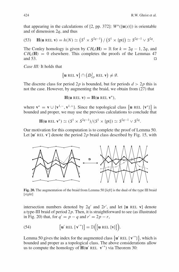
424 R.W. Ghrist et al.
that appearing in the calculations of [2, pp. 372]: Wu(u(s)) is orientableand of dimension 2q, and thus
H(u REL v) = h(N) (S1 × S2q−1
)/(S1 × pt) S2q−1 ∨ S2q.(53)
The Conley homology is given by CHk(H) = R for k = 2q − 1, 2q, andCHk(H) = 0 elsewhere. This completes the proofs of the Lemmas 47and 53. Case III: It holds that
u REL v ∩ (
D12p REL v
) = ∅.The discrete class for period 2p is bounded, but for periods d > 2p this isnot the case. However, by augmenting the braid, we obtain from (27) that
H(u REL v) = H(u REL v∗),
where v∗ = v ∪ v1,−, v1,+. Since the topological classu REL v∗ is
bounded and proper, we may use the previous calculations to conclude that
H(u REL v∗) (S1 × S2q−1)/(S1 × pt) S2q−1 ∨ S2q.
Our motivation for this computation is to complete the proof of Lemma 50.Let [u′ REL v′] denote the period 2p braid class described by Fig. 15, with
Fig. 20. The augmentation of the braid from Lemma 50 [left] is the dual of the type III braid[right]
intersection numbers denoted by 2q′ and 2r ′, and let [u REL v] denotea type-III braid of period 2p. Then, it is straightforward to see (as illustratedin Fig. 20) that, for q′ = p − q and r ′ = 2p − r,
[u′ REL [v′ ∗]] = D([
u REL [v]]).(54)
Lemma 50 gives the index for the augmented classu′ REL v′ ∗, which is
bounded and proper as a topological class. The above considerations allowus to compute the homology of H(u′ REL v′ ∗) via Theorem 30:

Morse theory on spaces of braids 425
CH∗(H(u′ REL v′ ∗)
) ∼= CH∗ (H(Du REL Dv))
∼= CH2p−∗ (H(u REL v))
∼= CH2p−∗ (H(u REL v∗))
∼=R : 2p − ∗ = 2q − 1, 2q
0 : else
∼=R : ∗ = 2q′, 2q′ + 1
0 : else.
(55)
The intersection numbers 2q′ and 2r ′ are exactly those of Lemma 50, com-pleting the proof.
11. Postlude
11.1. Extensions and questions: dynamics. There are several ways inwhich the basic machinery introduced in this paper can be generalized toother dynamical systems.
1. Scalar uniformly parabolic PDEs. Theorem 19 suggests strongly thatthe homotopy index for discretized braids extends to and agrees with ananalogous index for parabolic dynamics on spaces of smooth curves viauniformly parabolic PDE’s. This is true [23].
2. Periodicity in the range. Although we consider the anchor points to beinR, one may just as well constrain the anchor points to lie in S1 and work inthe universal cover. Such additional structure is used in the theory of annulustwist maps [2,7,36,37,42]. All of our results immediately carry over to thissetting. We note that compact-type boundary conditions necessarily follow.
3. Aperiodic dynamics. One can also extend the theory to include braiddiagrams with “infinite length” strands. To be more precise, consider braiddiagrams on the infinite 1-d lattice, and omit the spatial periodicity. In thiscontext several compactness issue come into play. To name a few: (a) theparabolic flows generated by aperiodic recurrence relations no longer liveon a finite dimensional space but on the infinite dimensional space ∞(R).See [2,3] for a case similar to this; (b) a priori, the Conley index should bereplaced with an infinite dimensional analogue such as that developed byRybakowski [52]. However, if one considers braid diagrams with finite wordmetric, the stabilization theory of Sect. 5 allows one to define the necessaryinvariants via the finite dimensional theory in this paper. This is not unlikethe procedure one can follow in the treatment of parabolic PDE’s [23].
4. Fixed boundary conditions. Our decision to use closed braid diagramsis motivated by applications in Lagrangian systems; however, one can alsofix the end points of the braid diagrams. In this setting one can definea braid invariant in the same spirit as is done for closed braids. The proof ofstabilization is not sensitive to the type of boundary conditions used. Such

426 R.W. Ghrist et al.
an extension of the theory to include fixed endpoints is useful in applicationsto parabolic PDE’s [23].5. Traveling waves and period orbits. The stationary solutions we find inthis paper are but the beginnings of a dynamical skeleton for the systemsconsidered. The next logical step would be to classify connecting orbitsbetween stationary solutions: several authors (e.g., [40]) have consideredthese problems analytically in the context of traveling wave phenomena inmonotone lattice dynamics. There is a precedent of using Conley indicesto prove existence theorems for connecting orbits (e.g., [47]): we anticipatethat such applications are possible in our setting. One could as well allowthe skeletal strands to be part of a periodic motion (in the case of non-exactrecurrence relations). In this setting one could look for both fixed points andperiodic solutions of a given braid class.6. Long-range coupling. Assume that the recurrence relations Ri are func-tions of the form Ri(ui−n, . . . , ui+n) for some n. Even if a strong mono-tonicity condition holds, ∂ jRi > 0 for all j = i the proof of Proposition 11still encounters a difficulty: two strands with a simple (codimension-one)tangency can have enough local crossings to negate the parabolic systems’separation. Such monotone systems do exhibit an ordering principle [3,26](initially nonintersecting strands will never intersect), but additional braid-ing phenomena are not automatically present.7. Higher-dimensional lattice dynamics. In parabolic PDE’s of spatial di-mension greater than one, the straightforward generalization of the lapnumber (number of connected components of an intersection of graphs)does not obey a monotonicity property (due to the fact that for graphs ofR
n with n > 1, critical points of non-zero index and co-index can passthrough each other). Finding a suitable form of dynamics which retainssome isolation remains an important and challenging problem.8. Arbitrary second-order Lagrangians. Our principal dynamical goal isto prove existence theorems for periodic orbits with a minimal amount ofassumptions, particularly “genericity” assumptions (which are, in practice,rarely verifiable). To this end, we have been successful for second-orderLagrangians modulo the twist assumption. Although this assumption isprobably satisfied in numerous contexts, we believe that it is not, strictlyspeaking, necessary. Its principal utility is in the reduction of the problem toa finite-dimensional recurrence relation. We believe that the forcing resultsproved in Sect. 8 are valid for all second-order Lagrangian systems. Seefor instance [31] for a result on that behalf. We propose that a version ofthe curve-shortening techniques in the spirit of Angenent [4] should yielda homotopy index for smooth curves to which our forcing theorems apply.
11.2. Extensions and questions: topology. The homotopy index is, asa topological invariant of braid pairs, utterly useless. Nevertheless, there istopological meaning intrinsic to this index, the precise topological interpre-tation of which is as yet unclear. One observes that the index captures some

Morse theory on spaces of braids 427
Morse-theoretic data about braid classes. Any topological interpretation iscertainly related to linking data of the free strands with the skeleton, asevidenced by the examples in this paper. Though the total amount of linkingshould provide some upper bound to the dimension of the homotopy index,linking numbers alone are insufficient to characterize the homotopy index.
We close with several related questions about the homotopy index itself.
1. Realization. It is clear that given any polynomial in t, there exists a braidpair whose homological Poincare polynomial agrees with this. [Idea: takeExample 3 of Sect. 4 and stack disjoint copies of the skeleton vertically,using as many free copies and strands as necessary to obtain the desiredhomology.] Can a realization theorem be proved for the homotopy indexitself? As a first step to this, consider replacing the real coefficients in thehomological index with integral coefficients. Does torsion ever occur? Webelieve not, with the possible exception of a Z2 torsion.
2. Product formulas and the braid group. Perhaps the most pressing problemfor the homotopy index is to determine a product formula for the concate-nation of two braids with compatible skeleta. This would eliminate the needfor computing the index via continuation to an integrable model system asin Sect. 10. However, since we work on spaces of closed braids, a productformula is not well-defined. The group structure on the braid group Bn doesnot extend naturally to a group structure on conjugacy classes: where one“cuts open” the braid to effect a gluing can change the resulting braid classdramatically. The one instance in which a product operation is natural isa power of a closed braid. Here, splitting the closed braid to an open braidand concatenating several copies then reclosing yields equivalent closedbraids independent of the representative of the conjugacy class chosen.Such a product/power formula, in conjunction with numerical methods ofindex computation effective in moderately low dimensions, would allowone to compute many invariants.
3. Improper and unbounded classes. In certain applications one also needsto deal with improper braid classes [u REL v]. To such classes one canalso assign an index. The interpretation of the index as a Morse theory willnot only depend on the topological data, but also on the behavior of theflow Ψt at Σ−. The simplest case is when Σ− ∩ ∂N consists of finitelymany points. This for example happens when u consists of only one strand.The homotopy index is then defined by the intrinsic definition in (15). Theinterpretation of the index and the associated Morse theory depends on thelinearization DΨt|Σ−∩∂N . The definition of the index in the case of morecomplicated sets Σ− ∩ ∂N and the Morse theoretic interpretation will besubject of future study. Similar considerations hold for unbounded classes.
4. General braids. The types of braids considered in this paper are positivebraids. Naturally, one wishes to extend the ideas to all braids; however,several complications arise. First, passing to discretized braids is invalid –knowing the anchor points is insufficient data for reconstructing the braid.Second, compactness is troublesome – one cannot merely bound braid
428 R.W. Ghrist et al.
classes via augmentation. We can model general braids dynamically usingrecurrence relations with nearest neighbor coupling allowing “positive”, or“negative” interaction. This idea appears in the work of LeCalvez [36,37]and can be translated to our setting via a change of variables – coordinateflips – of which our duality operator D is a particular example. Howeverthe compactness and discretization issues remain. LeCalvez works in thesetting of annulus maps, where one can circumvent these problems: thegeneral setting is more problematic.5. Hamiltonian vs. Lagrangian. One approach to extending to arbitrarybraids would be to switch from a Lagrangian setting to a Hamiltoniansetting. Consider an S1 family of Hamiltonians Ht on a symplectic surface(M2, ω) which has a “skeleton” of periodic orbits braided in M×S1. Adding“free” braid strands, one could define a relative Floer index for the systemwhich should detect whether the free strands are forced to exist as periodicorbits.
Appendix A. Construction of parabolic flows
In this appendix, we construct particular parabolic flows on braid diagramsin order to carry out the continuation arguments for the well-definedness ofthe Conley index for proper braid diagrams. The constructions are explicitand are generated by recurrence relations R = (Ri)i∈Z, with Ri+d = Ri ,which are of the form:
Ri(r, s, t) = ai(r, s)+ bi(s, t)+ ci(s), i = 1, ..., d,(56)
with ai, bi, ci ∈ C1(R), and ∂ai∂r (r, s) > 0, ∂bi
∂t (s, t) ≥ 0 for all (r, s, t) ∈ R3.By definition, such recurrence relations are parabolic.
Lemma 55. For any v ∈ Dmd there exists a parabolic flow Ψt under which
v is stationary.
Proof. In order to have Ψt(v) = v, the sequences vα need to satisfyRi(v
αi−1, v
αi , vα
i+1) = 0, for some parabolic recurrence relation. We willconstruct R by specifying the appropriate functions ai, bi , ci as above. Inthe construction to follow, the reader should think of the anchor points vα
i of the fixed braid v as constants.
For each i such that the values vαi α are distinct, one may choose
ai(r, s) = r, bi(s, t) = t, and ci(s) to be any C1 function which interpolatesthe defined values
ci(vα
i
) := −(vα
i−1 + vαi+1
).
This generates the desired parabolic flow.In the case where there are several strands α1, α2, . . . αn for which
vα j
i = v∗ are all equal, the former construction is invalid: ci is not well-defined. According to Definition 4, we have for each α j = αk (v
α j
i−1 −

Morse theory on spaces of braids 429
vαki−1)(v
α j
i+1 − vαki+1) < 0. This implies that if we order the α j j so that
vα1i−1 < v
α2i−1 < · · · < v
αni−1, then the corresponding sequence vα j
i+1 j sat-isfies v
αni+1 < v
αn−1i+1 < · · · < v
α1i+1. From Lemma 56 below, there exist
increasing functions f and g such that
f(v
α j
i−1
)− f(v
αki−1
) = g(v
αki+1
)− g(v
α j
i+1
) ∀ j, k.
Define ai and bi in the following manner: set ai(r, v∗) := f(r) and bi(v∗, t)
:= g(t). Thus it follows that there exists a well defined value
ci(v∗) := − (
f(v
α j
i−1
)+ g(v
α j
i+1
))which is independent of j. For any other strands α′, repeat the procedure,defining the slices ai(r, vα′
i ), bi(vα′i , t) and the points ci(v
α′i ), choosing new
functions f and g if necessary. To extend these functions to global functionsai(r, s) and bi(s, t), simply perform a C1 homotopy in s without changingthe monotonicity in the r and t variables: e.g., on the interval [vα
i , vα′i ],
choose a monotonic function ξ(s) for which ξ(vαi ) = ξ ′(vα
i ) = ξ ′(vα′i ) = 0
and ξ(vα′i ) = 1. Then set
ai(r, s) := (1− ξ(s))ai(r, vα
i
)+ ξ(s)ai(r, vα′
i
).
Such a procedure, performed on the appropriate s-intervals, yields a smoothr-monotonic interpolation. Repeat with bi(s, t). Finally, choose any functionci(s) which smoothly interpolates the preassigned values. These choices ofai , bi and ci give the desired recurrence relation, and consequently theparabolic flow Ψt . Lemma 56. Given two sequences of increasing real numbers x1 < x2 <· · · < xn and y1 < y2 < · · · < yn, there exist a pair of strictly increasingfunctions f and g such that
f(x j)− f(xk) = g(y j)− g(yk) ∀ j, k.(57)
Proof. Induct on n, noting the triviality of the case n = 1. Given increasingsequences (xi)
N+11 and (yi)
N+11 , choose functions f and g which satisfy (57)
for j, k ≤ N: this is a restriction on f and g only for values in [x1, xN ] sinceoutside of this domain the functions can be arbitrary as long as they areincreasing. Thus, modify f and g outside this interval to satisfy
f(xN+1) = f(xN )+ C ; g(yN+1) = g(yN )+ C,
for some fixed constant C > 0. These functions satisfy (57) for all jand k. Lemma 57. For any pair of equivalent braids [u(0)] = [u(1)], there existsa path u(λ) in Dn
d and a continuous family of parabolic flows Ψtλ, such that
Ψtλ(u(λ)) = u(λ), for all λ ∈ [0, 1].

430 R.W. Ghrist et al.
Proof. Given u any point in Dnd , consider any parabolic recurrence relation
Ru which fixes u and which is strictly monotonic in r and t. From theproof of Lemma 55, Ru exists. For every braid u′ sufficiently close to u,there exists φ a near-identity diffeomorphism of Dn
d which maps u to u′.The recurrence relation Ru φ−1 fixes u′ and is still parabolic since φcannot destroy monotonicity. Choosing a short smooth path φt of suchdiffeomorphisms to ID proves the lemma on small neighborhoods in Dn
d ,which can be pieced together to yield arbitrary paths.
References
1. Akmediev, N.N., Buryak, A.V., Karlsson, M.: Radiationless optical solitons with oscil-lating tails. Optim. Commun. 110, 540–544 (1994)
2. Angenent, S.B.: The periodic orbits of an area preserving Twist-map. Commun. Math.Phys. 115, 353–374 (1988)
3. Angenent, S.B.: Monotone recurrence relations, their Birkhoff orbits and topologicalentropy. Ergodic Theory Dyn. Syst. 10, 15–41 (1990)
4. Angenent, S.B.: Curve Shortening and the topology of closed geodesics on surfaces.Preprint 2000
5. Angenent, S.B.: The zero set of a solution of a parabolic equation. J. Reine Angew.Math. 390, 79–96 (1988)
6. Angenent, S.B., Van den Berg, J.B., Vandervorst, R.C.: Contact and noncontact energyhypersurfaces in second order Lagrangian systems. Preprint 2001
7. Aubry, S., LeDaeron, P.Y.: The Frenkel-Kontorova model and its extensions. PhysicaD 8, 381–422 (1983)
8. Birman, J.: Braids, links and the mapping class group. Ann. Math. Stud. 82 (1975).Princeton Press
9. Boyland, P.: Topological methods in surface dynamics. Topology Appl. 58, 223–298(1994)
10. Brunovsky, P., Fiedler, B.: Connecting orbits in scalar reaction-diffusion equations.Dyn. Rep. 1, 57–89 (1988)
11. Conley, C.: Isolated invariant sets and the Morse index. CBMS Reg. Conf. Ser. Math.38 (1978), published by the AMS
12. Conley, C., Fife, P.: Critical manifolds, travelling waves, and an example from popula-tion genetics. J. Math. Biol. 14, 159–176 (1982)
13. Conley, C., Zehnder, E.: The Birkhof-Lewis fixed point theorem and a conjecture ofV.I. Arnol’d, Invent. Math. 73, 33–49 (1983)
14. Conley, C., Zehnder, E.: Morse-type index theory for flows and periodic solutions forHamiltonian equations. Comm. Pure Appl. Math. 37, 207–253 (1984)
15. Dancer, N.: Degenerate critical points, homotopy indices and Morse inequalities.J. Reine Angew. Math. 350, 1–22 (1984)
16. Eliashberg, Y., Givental, A., Hofer, H.: An introduction to symplectic field theory.Geom. Func. Anal., Special Volume II, 560–673 (2000)
17. Floer, A.: A refinement of the Conley index and an application to the stability ofhyperbolic invariant sets. Ergodic Theory Dyn. Sys. 7, 93–103 (1987)
18. Fiedler, B., Mallet-Paret, J.: A Poincare-Bendixson theorem for scalar reaction diffusionequations. Arch. Ration. Mech. Anal. 107, 325–345 (1989)
19. Fiedler, B., Rocha, C.: Realization of meander permutations by boundary value prob-lems. J. Differ. Equations 156, 282–308 (1999)
20. Fiedler, B., Rocha, C.: Orbit equivalence of global attractors of semilinear parabolicdifferential equations. Trans. Am. Math. Soc. 352, 257–284 (2000)
21. Fusco, G., Oliva, W.M.: Transversality between invariant manifolds of periodic orbitsfor a class of monotone dynamical systems. J. Dyn. Differ. Equations 2, 1–17 (1990)

Morse theory on spaces of braids 431
22. Fusco, G., Oliva, W.: Jacobi matrices and transversality. Proc. R. Soc. Edinb. Sect. AMath. 109, 231–243 (1988)
23. Ghrist, R., Vandervorst, R.C.: Scalar parabolic dynamics via braids. In progress24. Ghrist, R., Vandervorst, R.C.: Braids and scalar parabolic PDEs. In: Proceedings of
New Directions in Dynamics Systems, Kyoto 200225. Hansen, V.L.: Braids and Coverings: Selected Topics. Cambridge University Press 198926. Hirsch, M.: Systems of differential equations which are competitive or cooperative, I:
Limit sets. SIAM J. Math. Anal. 13, 167–179 (1982).27. Hofer, H.: Pseudo-holomorphic curves and the Weinstein conjecture in dimension three.
Invent. Math. 114, 515–563 (1993)28. Hofer, H., Zehnder, E.: Symplectic invariants and Hamiltonian dynamics. Birkhäuser
199329. Hulshof, J., Van den Berg, J.B., Vandervorst, R.C.A.M.: Traveling waves for fourth-
order semilinear parabolic equations. SIAM J. Math. Anal. 32, 1342–1374 (2001)30. Kalies, W.D., Holmes, P.J.: On a dynamical model for phase transformation in nonlinear
elasticity. Pattern formation: symmetry methods and applications (Waterloo, ON, 1993).Fields Inst. Commun. 5, 255–269 (1996). Providence, RI: Am. Math. Soc.
31. Kalies, W.D., Vandervorst, R.C.A.M.: Closed characteristics of second order La-grangians. Preprint 2002
32. Kalies, W.D., Kwapisz, J., Vandervorst, R.C.A.M.: Homotopy classes for stable con-nections between Hamiltonian saddle-focus equilibria. Commun. Math. Phys. 193,337–371 (1998)
33. Kalies, W.D., Kwapisz, J., Van den Berg, J.B., Vandervorst, R.C.A.M.: Homotopyclasses for stable periodic and chaotic patterns in fourth-order Hamiltonian systems.Commun. Math. Phys. 214, 573–592 (2000)
34. Kwapisz, J.: Uniqueness of the stationary wave for the extended Fisher-Kolmogorovequation. Preprint (1997). J. Differ. Equations 165, 235–253 (2000)
35. Kwapisz, J.: Personal communication36. LeCalvez, P.: Propriete dynamique des diffeomorphismes de l’anneau et du tore.
Asterique 204 (1991)37. LeCalvez, P.: Decomposition des diffeomorphismes du tore en applications deviant la
verticale. Mem. Soc. Math. Fr., Nouv. Sér. (79) (1999)38. Leizarowitz, A., Mizel, V.J.: One-dimensional infinite-horizon variational problems
arising in continuum mechanics. Arch. Ration. Mech. Anal. 106, 161–194 (1989)39. Mallet-Paret, J., Smith, H.L.: The Poincare-Bendixson theorem for monotone cyclic
feedback systems. J. Dyn. Differ. Equations 2, 367–421 (1990)40. Mallet-Paret, J.: The global structure of traveling waves in spatially discrete dynamical
systems. J. Dyn. Differ. Equations 11, 49–127 (1999)41. Matano, H.: Nonincrease of the lap-number of a solution for a one dimensional semi-
linear parabolic equation. J. Fac. Sci. Univ. Tokyo 29, 401–441 (1982)42. Mather, J.N.: Existence of quasi-periodic orbits for twist diffeomorphisms of the annu-
lus. Topology 21, 457–467 (1982)43. Mather, J.N.: Amount of rotation about a point and the morse index. Commun. Math.
Phys. 94, 141–153 (1984)44. McCord, C.: Poincare-Lefschetz duality for the homology Conley index. Trans. Am.
Math. Soc. 329, 233–252 (1992)45. Middleton, A.: Asymptotic uniqueness of the sliding state for charge-density waves.
Phys. Rev. Lett. 68, 670–673 (1992)46. Milnor, J.: Morse Theory. Ann. Math. Stud. 51. Princeton Press 196347. Mischaikow, K.: Recent developments in Conley index theory. Springer Lecture Notes
Math. 1609 (1995)48. Moser, J.: Monotone twist mappings and the calculus of variations. Ergodic Theory
Dyn. Syst. 6, 401–413 (1986)49. Peletier, L.A., Troy, W.C.: Higher order patterns: higher order models in physics and
mechanics. Birkhäuser 2001

432 R.W. Ghrist et al.
50. Peletier, L.A., Troy, W.C.: Multibump periodic traveling waves in suspension bridges.Proc. R. Soc. Edinb. 128A (1998), 631–659
51. Peletier, L.A., Troy, W.C., Van den Berg, J.B.: Global branches of multi bump periodicsolutions of the Swift-Hohenberg equation. Arch. Ration. Mech. Anal. 158, 91–153(2001)
52. Rybakowski, K.: The homotopy index and partial differential equations. Universitext.Berlin: Springer-Verlag 1987
53. Smillie, J.: Competitive and cooperative tridiagonal systems of differential equations.SIAM J. Math. Anal. 15, 531–534 (1984)
54. Sturm, C.: Mémoire sur une classe d’equations à différences partielles. J. Math. PureAppl. 1, 373–444 (1836)
55. Truskinovsky, L., Zanzotto, G.: Ericksen’s bar revisited: energy wiggles. J. Mech. Phys.Solids 44, 1371–1408 (1996)
56. Van Moerbeke, P.: The spectrum of Jacobi matrices. Invent. Math. 37, 45–81 (1976)57. Van den Berg, J.B.: The phase-plane picture for a class of fourth-order conservative
differential equations. Preprint (1998). J. Differ. Equations 161, 110–153 (2000)58. Van den Berg, J.B., Vandervorst, R.C.A.M.: Fourth order conservative Twist systems:
simple closed characteristics. Trans. Am. Math. Soc. 354, 1383–1420 (2002)59. Vassiliev, V.: Complements of discriminants of smooth maps: topology and applications.
Translated from the Russian by B. Goldfarb, Providence, RI: Am. Math. Soc. 199260. Wilson, F.W., Yorke, J.A.: Lyapunov functions and isolating blocks. J. Differ. Equations
13, 106–123 (1973)