mortgage insurance fund: cash flow npv from forward · fiscal year 2017 independent actuarial...
TRANSCRIPT

3109 Cornelius Drive
Bloomington, IL 61704 309.807.2300
pinnacleactuaries.com
Commitment Beyond Numbers
Roosevelt C. Mosley, Jr., FCAS, MAAA [email protected]
Direct: 309.807.2330
November 10, 2017
Dana Wade
General Deputy Assistant Secretary
Office of Housing
U.S. Department of Housing and Urban Development
451 Seventh Street, S.W., Room 9100
Washington, D.C. 20410
Dear Ms. Wade:
Pinnacle Actuarial Resources, Inc. (Pinnacle) has completed the final report for the Fiscal Year 2017
Independent Actuarial Review of the Mutual Mortgage Insurance Fund Forward Loans. The attached
report details our estimate of the Cash Flow Net Present Value for fiscal year 2017.
Roosevelt C. Mosley, Jr., FCAS, MAAA and Thomas R. Kolde, FCAS, MAAA are responsible for the
content and conclusions set forth in the report. We are Fellows of the Casualty Actuarial Society and
Members of the American Academy of Actuaries, and are qualified to render the actuarial opinion
contained herein.
It has been a pleasure working with you and your team to complete this study. We are available for any
questions or comments you have regarding the report and its conclusions.
Respectfully Submitted,
Roosevelt C. Mosley, Jr. FCAS, MAAA Thomas R. Kolde, FCAS, MAAA
Principal and Consulting Actuary Consulting Actuary

3109 Cornelius Drive Bloomington, IL 61704
309.807.2300 pinnacleactuaries.com
Commitment Beyond Numbers
FiscalYear2017IndependentActuarialReviewoftheMutualMortgage
InsuranceFund:CashFlowNetPresentValuefromForwardMortgageInsurance‐
In‐Force
November 10, 2017

Fiscal Year 2017 Independent Actuarial Review of the Mutual Mortgage Insurance Fund: Cash Flow NPV from Forward
Mortgage Insurance‐In‐Force
Commitment Beyond Numbers
Table of Contents
Summary of Findings ................................................................................................................................................. 1
Executive Summary ................................................................................................................................................... 5
Impact of Economic Forecasts ............................................................................................................................... 5
Distribution and Use .................................................................................................................................................. 7
Reliances and Limitations .......................................................................................................................................... 7
Section 1: Introduction .............................................................................................................................................. 9
Scope ..................................................................................................................................................................... 9
Background .......................................................................................................................................................... 10
Report Structure .................................................................................................................................................. 10
Section 2: Summary of Findings .............................................................................................................................. 11
Fiscal Year 2017 Cash Flow NPV Estimate ........................................................................................................... 11
Section 3: Cash Flow NPV Based on Alternative Scenarios ..................................................................................... 14
Moody’s Baseline Assumptions ........................................................................................................................... 14
Stronger Near‐Term Growth Scenario ................................................................................................................ 15
Slower Near‐Term Growth Scenario ................................................................................................................... 15
Moderate Recession Scenario ............................................................................................................................. 15
Protracted Slump ................................................................................................................................................. 15
Below‐Trend Long‐Term Growth ......................................................................................................................... 15
Stagflation ............................................................................................................................................................ 16
Next‐Cycle Recession ........................................................................................................................................... 16
Low Oil Price ........................................................................................................................................................ 16
Summary of Alternative Scenarios ...................................................................................................................... 16
Stochastic Simulation .......................................................................................................................................... 17
Sensitivity Tests of Economic Variables ............................................................................................................... 19
Section 4: Summary of Methodology ...................................................................................................................... 22
Data Sources ........................................................................................................................................................ 22
Data Processing – Mortgage Level Modeling (Appendix A) ................................................................................ 22

Fiscal Year 2017 Independent Actuarial Review of the Mutual Mortgage Insurance Fund: Cash Flow
Net Present Value from Forward Mortgage Insurance‐In‐Force
November 10, 2017 Page ii
Pinnacle Actuarial Resources, Inc.
Data Reconciliation .............................................................................................................................................. 23
Specification of Mortgage Transition Models (Appendix B) ............................................................................... 27
Estimation Sample ............................................................................................................................................... 28
Loss Severity Model (Appendix C) ....................................................................................................................... 29
Cash Flow Projections (Appendix E) .................................................................................................................... 29
Appendices .............................................................................................................................................................. 31
Appendix A: Data – Sources, Processing and Reconciliation ................................................................................... 32
Data Sources ........................................................................................................................................................ 32
Data Processing – Mortgage Level Modeling ...................................................................................................... 33
Data Reconciliation .............................................................................................................................................. 33
Appendix B: Transition Models ............................................................................................................................... 38
Section 1: Model Specification ............................................................................................................................ 38
Multinomial Logistic Regression Theory and Model Specification.................................................................. 39
Section 2: Transition Model Explanatory Variables ............................................................................................. 41
Section 3: Model Validation ................................................................................................................................ 42
Current Transition Models .............................................................................................................................. 43
Default Transition Models ............................................................................................................................... 46
Appendix C: Loss Severity Models ........................................................................................................................... 51
Model Specifications ........................................................................................................................................... 51
Net Loss Severity Model Specification ............................................................................................................ 53
Estimation Sample ........................................................................................................................................... 55
Explanatory Variables .......................................................................................................................................... 56
Model Validation ................................................................................................................................................. 56
Appendix D: Economic Scenarios ............................................................................................................................ 63
Alternative Scenarios ........................................................................................................................................... 63
Graphical Depiction of the Scenarios .................................................................................................................. 64
Stochastic Simulations ......................................................................................................................................... 66
Historical Data ................................................................................................................................................. 67
Modeling Techniques ...................................................................................................................................... 70
1‐Year CMT Rate .............................................................................................................................................. 70

Fiscal Year 2017 Independent Actuarial Review of the Mutual Mortgage Insurance Fund: Cash Flow
Net Present Value from Forward Mortgage Insurance‐In‐Force
November 10, 2017 Page iii
Pinnacle Actuarial Resources, Inc.
Additional Interest Rate Models ..................................................................................................................... 72
HPA .................................................................................................................................................................. 73
Unemployment Rate ....................................................................................................................................... 75
Gross Domestic Product .................................................................................................................................. 76
Final Simulation Selection ............................................................................................................................... 76
Appendix E: Cash Flow Analysis ............................................................................................................................... 77
Introduction ......................................................................................................................................................... 77
Definitions ........................................................................................................................................................... 77
Cash Flow Components ....................................................................................................................................... 78
MIP .................................................................................................................................................................. 78
Upfront MIP ..................................................................................................................................................... 80
Annual Premium .............................................................................................................................................. 81
Refunded MIP .................................................................................................................................................. 81
Losses Associated with Claims ......................................................................................................................... 81
Loss Mitigation Expenses ................................................................................................................................. 82
Net Present Value ................................................................................................................................................ 82

Fiscal Year 2017 Independent Actuarial Review of the Mutual Mortgage Insurance Fund: Cash Flow NPV from Forward
Mortgage Insurance‐In‐Force
Commitment Beyond Numbers
Summary of Findings This report presents the results of Pinnacle Actuarial Resources, Inc.’s (Pinnacle’s) independent actuarial review
of the Cash Flow Net Present Value (NPV) associated with forward mortgages insured by the Mutual Mortgage
Insurance Fund (MMIF) for fiscal year 2017. The Cash Flow NPV associated with Home Equity Conversion
Mortgages (HECMs) are analyzed separately and are excluded from this report. In the remainder of this report,
the term MMIF refers to forward mortgages and excludes HECMs.
Below we summarize the findings associated with each of the required deliverables.
Deliverable 1: The Actuary’s conclusion regarding the reasonableness of Federal Housing Administration’s
(FHA’s) estimate of Cash Flow Net Present Value from Forward Mortgage Insurance‐In‐Force as presented in
FHA’s Annual Report to Congress and the Actuary’s best estimate of the range of reasonable estimates,
including the 90th, 95th and 99th percentiles.
As of the end of Fiscal Year 2017, Pinnacle’s Actuarial Central Estimate (ACE) of the MMIF Cash Flow NPV is
$1.893 billion.
Pinnacle’s ACE is based on the Economic Assumption for the 2018 Budget Fall Baseline from the Office of
Management and Budget (OMB Economic Assumptions). Pinnacle also estimated Cash Flow NPV outcomes
based on economic scenarios from Moody’s Analytics (Moody's). The Cash Flow NPV results based on these
scenarios are shown in Table 1.
Table 1: Range of Cash Flow NPV Outcomes Based on Moody’s Scenarios
The range of results based on the Moody’s estimates is negative $36.31 billion to positive $8.70 billion.
In addition, Pinnacle has estimated a range of outcomes based on 100 randomly generated stochastic
simulations of key economic variables. Based on these simulations, we estimate that the range of reasonable
Cash Flow NPV estimates is negative $5.0 billion to positive $8.5 billion. This range is based on an 80% likelihood
Fiscal Year 2017 Independent Actuarial Review of the Mutual Mortgage Insurance Fund: Cash Flow
Net Present Value from Forward Mortgage Insurance‐In‐Force
November 10, 2017 Page 2
Pinnacle Actuarial Resources, Inc.
that the ultimate Cash Flow NPV will fall within the lower and upper bound of the range.
The 90th, 95th and 99th percentiles of the stochastic simulations are shown below:
90th percentile: $8.5 billion
95th percentile: $11.9 billion
99th percentile: $13.7 billion
The Cash Flow NPV estimate provided by FHA to be used in the FHA’s Annual Report to Congress is $1.4 billion.
Based on Pinnacle’s Actuarial Central Estimate and range of reasonable estimates, we conclude that the FHA
estimate of Cash Flow NPV to be used in the FHA’s Annual Report to Congress is reasonable.
Deliverable 2: The Actuary’s best estimate and range of reasonable estimates of Cash Flow Net Present Value
by cohort from Forward (Home Equity Conversion) Mortgage Insurance‐In‐Force as presented in FHA’s Annual
Report to Congress.
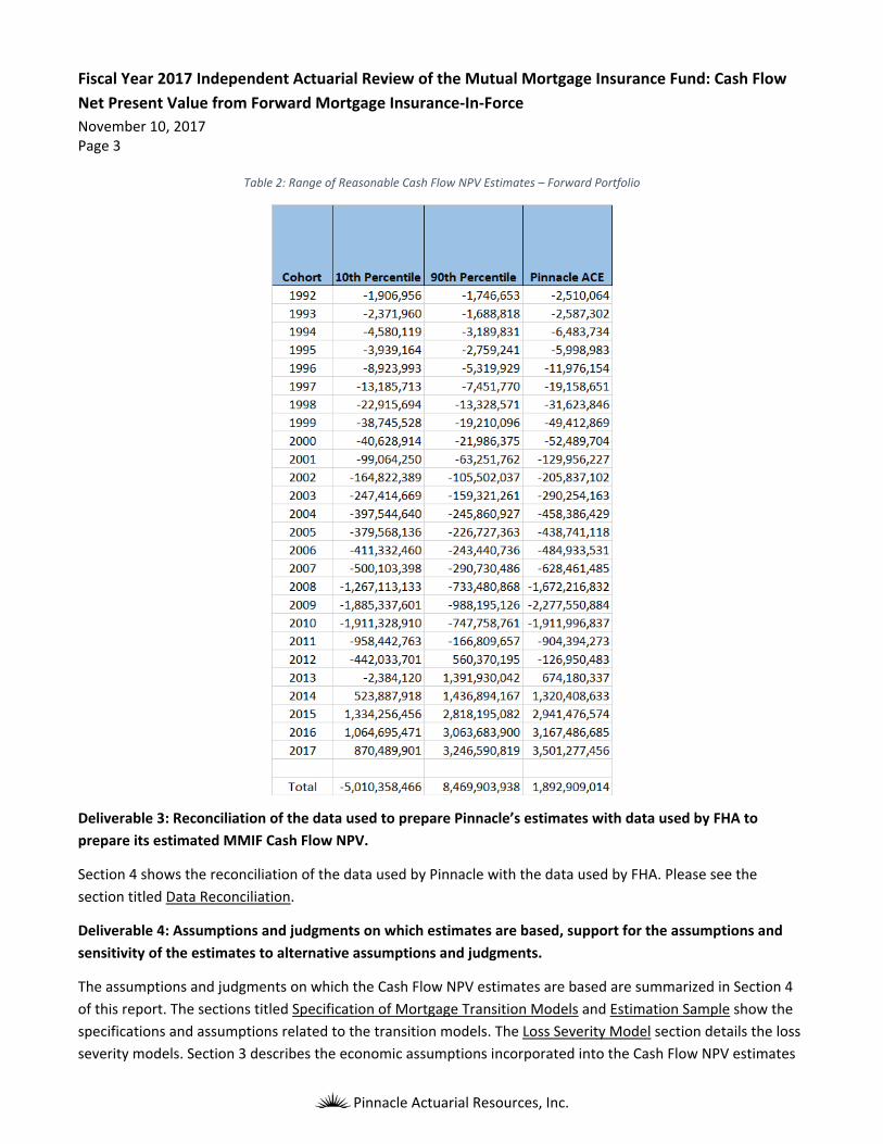
Pinnacle’s range of reasonable estimates of the Cash Flow NPV by cohort are shown below. The range of
estimates are based on the stochastic simulation results.
Fiscal Year 2017 Independent Actuarial Review of the Mutual Mortgage Insurance Fund: Cash Flow
Net Present Value from Forward Mortgage Insurance‐In‐Force
November 10, 2017 Page 3
Pinnacle Actuarial Resources, Inc.
Table 2: Range of Reasonable Cash Flow NPV Estimates – Forward Portfolio
Deliverable 3: Reconciliation of the data used to prepare Pinnacle’s estimates with data used by FHA to
prepare its estimated MMIF Cash Flow NPV.
Section 4 shows the reconciliation of the data used by Pinnacle with the data used by FHA. Please see the
section titled Data Reconciliation.
Deliverable 4: Assumptions and judgments on which estimates are based, support for the assumptions and
sensitivity of the estimates to alternative assumptions and judgments.
The assumptions and judgments on which the Cash Flow NPV estimates are based are summarized in Section 4
of this report. The sections titled Specification of Mortgage Transition Models and Estimation Sample show the
specifications and assumptions related to the transition models. The Loss Severity Model section details the loss
severity models. Section 3 describes the economic assumptions incorporated into the Cash Flow NPV estimates

Fiscal Year 2017 Independent Actuarial Review of the Mutual Mortgage Insurance Fund: Cash Flow
Net Present Value from Forward Mortgage Insurance‐In‐Force
November 10, 2017 Page 4
Pinnacle Actuarial Resources, Inc.
and the sensitivity of the estimates to alternative economic scenarios. Lastly, the Cash Flow Projections section
of Section 4 summarizes the assumptions associated with the cash flow analysis.
Deliverable 5: Narrative component that provides detail to explain to FHA and HUD management and
auditors, OMB and Congressional offices the findings and their significance, and technical component that
traces the analysis from the data to the conclusions.
Sections 1 and 2 provide an explanation of the findings and discusses the significance of the findings. Also,
Section 4 traces the analysis from data to conclusions.
Deliverable 6: Commentary on the likelihood of risks and uncertainties that could result in material adverse
changes in the condition of the MMIF as measured by the Cash Flow NPV.
Section 3 provides a discussion of the economic conditions that could result in material adverse change to the
Cash Flow NPV.

Fiscal Year 2017 Independent Actuarial Review of the Mutual Mortgage Insurance Fund: Cash Flow
Net Present Value from Forward Mortgage Insurance‐In‐Force
November 10, 2017 Page 5
Pinnacle Actuarial Resources, Inc.
Executive Summary The 1990 Cranston‐Gonzalez National Affordable Housing Act (NAHA) requires an independent actuarial analysis
of the economic value of the FHA and Department of Housing and Urban Development’s (HUD’s) MMIF. Enacted
on July 30, 2008, the Housing and Economic Recovery Act of 2008 (HERA) moved the requirement for an
independent actuarial review into 12 USC 1708(a)‐(4).
HERA also moved several additional programs into the MMIF. One of them, Home Equity Conversion Mortgages,
which are reverse mortgages, are analyzed separately and are excluded from this report. In the remainder of
this report, the term MMIF refers to forward mortgages and excludes HECMs.
The primary purpose of this actuarial analysis is to estimate the Cash Flow NPV of the current book of business.
We have calculated a range of estimates using economic projections from the OMB Economic Assumptions for
Fiscal Year 2018, nine economic projection scenarios from Moody’s and a stochastic simulation approach to test
variation around economic scenarios.
Based on our analysis, we estimate that the Cash Flow NPV as of the end of fiscal year 2017 is $1.893 billion. We
also estimate that the reasonable range of Cash Flow NPV is between negative $5.0 billion and positive $8.5
billion.
Impact of Economic Forecasts
The Cash Flow NPV of the MMIF depends on many factors. One of the most important set of factors is the
prevailing economic conditions over the next 30 years, and most critically during the next 10 years. We
incorporate the most significant factors in the U.S. economy affecting the performance of the mortgages insured
by the MMIF through the use of the following variables in our models:
30‐year fixed‐rate home mortgage effective rates
10‐year Constant Maturity Treasury (CMT) rates
1‐year CMT rates
Housing price index (HPI)
Unemployment rates
Gross Domestic Product (GDP)
The projected Cash Flow NPV of FHA’s books of business is affected by changes in these economic variables. The
ACE results in this report is derived from using the OMB Economic Assumptions.
We also estimated the Cash Flow NPV of the MMIF under nine additional economic scenarios from Moody’s.
These scenarios are:
Moody’s Baseline
Stronger Near‐Term Growth
Slower Near‐Term Growth

Fiscal Year 2017 Independent Actuarial Review of the Mutual Mortgage Insurance Fund: Cash Flow
Net Present Value from Forward Mortgage Insurance‐In‐Force
November 10, 2017 Page 6
Pinnacle Actuarial Resources, Inc.
Moderate Recession
Protracted Slump
Below‐Trend Long‐Term Growth
Stagflation
Next‐Cycle Recession
Low Oil Price
These scenarios do not represent the full range of possible future economic paths. They represent a
considerable variation of economic conditions. Therefore they provide insights into the projected Cash Flow NPV
of the MMIF under a range of economic environments.
The summary of estimated Cash Flow NPV resulting from each approach is shown in Table 3.
Table 3: Projected Forward Cash Flow NPV Using Alternative Economic Scenarios
We also randomly generated 100 stochastic simulations of key economic variables. Based on these simulations,
we estimate that the range of reasonable Cash Flow NPV estimates is negative $5.0 billion to positive $8.5
billion. This range is based on an 80% likelihood that the ultimate Cash Flow NPV will fall within the lower and
upper bound of the range.

Fiscal Year 2017 Independent Actuarial Review of the Mutual Mortgage Insurance Fund: Cash Flow
Net Present Value from Forward Mortgage Insurance‐In‐Force
November 10, 2017 Page 7
Pinnacle Actuarial Resources, Inc.
Distribution and Use This report is being provided to FHA for its use and the use of makers of public policy in evaluating the Cash Flow
NPV of the MMIF. Permission is hereby granted for its distribution on the condition that the entire report,
including the exhibits and appendices, is distributed rather than any excerpt. Pinnacle also acknowledges that
excerpts of this report will be used in preparing summary comparisons for FHA’s Annual Report to Congress, and
permission is granted for this purpose as well. We are available to answer any questions that may arise
regarding this report.
Any third parties receiving the report should recognize that the furnishing of this report is not a substitute for
their own due diligence and should place no reliance on this report or the data contained herein that would
result in the creation of any duty or liability by Pinnacle to the third party.
Our conclusions are predicated on a number of assumptions as to future conditions and events. These
assumptions, which are documented in subsequent sections of the report, must be understood in order to place
our conclusions in their appropriate context. In addition, our work is subject to inherent limitations, which are
also discussed in this report.
Reliances and Limitations Listed in Section 4 are the data sources Pinnacle has relied on in our analysis. We have relied on the accuracy of
these data sources in our calculations. If it is subsequently discovered that the underlying data or information is
erroneous, then our calculations would need to be revised accordingly.
We have relied on a significant amount of data and information from external sources without audit or
verification. This includes economic data projected over the next 30 years from Moody’s and the OMB.
However, we did review as many elements of the data and information as practical for reasonableness and
consistency with our knowledge of the mortgage insurance industry. It is possible that the historical data used to
develop our estimates may not be predictive of future default and loss experience. We have not anticipated any
extraordinary changes to the legal, social or economic environment which might affect the number or cost of
mortgage defaults beyond those contemplated in the economic scenarios described in this report. To the extent
that the realized experience deviates significantly from these assumptions, the actual results may differ, perhaps
significantly, from projected results.
The predictive models used in this analysis are based on a theoretical framework and certain assumptions. This
model structure predicts the rates of default, claim, loss and prepayment based on a number of individual
mortgage characteristics and economic variables. The models are built using predictive modeling techniques,
analyzing data from actual historical experience of FHA‐insured mortgages. The parameters of the predictive
models are estimated over a wide variety of mortgages originated since 1975 and their performance under the
range of economic conditions and mortgage market environments experienced during the past 40 years. The
predictive models are combined with assumptions about future behavior of current mortgage endorsements
and certain key economic assumptions to produce future projections of the performance of the existing

Fiscal Year 2017 Independent Actuarial Review of the Mutual Mortgage Insurance Fund: Cash Flow
Net Present Value from Forward Mortgage Insurance‐In‐Force
November 10, 2017 Page 8
Pinnacle Actuarial Resources, Inc.
mortgages insured by the MMIF.
Pinnacle is not qualified to provide formal legal interpretation of federal legislation or FHA policies and
procedures. The elements of this report that require legal interpretation should be recognized as reasonable
interpretations of the available statutes, regulations and administrative rules.
Fiscal Year 2017 Independent Actuarial Review of the Mutual Mortgage Insurance Fund: Cash Flow
Net Present Value from Forward Mortgage Insurance‐In‐Force
November 10, 2017 Page 9
Pinnacle Actuarial Resources, Inc.
Section 1: Introduction
Scope
FHA has engaged Pinnacle to perform the annual independent actuarial study of the MMIF. This study is
required by 12 USC 1708(a)‐(4) and must be completed in compliance with the Federal Credit Reform Act as
implemented and all applicable Actuarial Standards of Practice (ASOPs). This study provides an analysis of the
Cash Flow NPV of the MMIF as of September 30, 2017.
The MMIF is a group of accounts of the federal government which records transactions associated with the
FHA’s guarantee programs for single family mortgages. Currently, the FHA insures approximately 7.83 million
forward mortgages under the MMIF and 440,000 reverse mortgages under the HECM program.
Per 12 USC 1711‐(f), the FHA must endeavor to ensure that the MMIF maintains a capital ratio of not less than
2.0%. The capital ratio is defined as the ratio of capital to the MMIF obligations on outstanding mortgages
(insurance‐in‐force, or IIF). Capital is defined as cash available to the MMIF plus the Cash Flow NPV of all future
cash outflows and inflows that are expected to result from the mortgages currently insured by the MMIF.
The deliverables included in this study are:
1. The Actuary’s conclusion regarding the reasonableness of FHA’s estimate of Cash Flow Net Present Value from Forward (Home Equity Conversion) Mortgage Insurance‐In‐Force as presented in FHA’s Annual Report To Congress and the Actuary’s best estimate of the range of reasonable estimates, including the 90th, 95th and 99th percentiles.
2. The Actuary’s best estimate and range of reasonable estimates of Cash Flow Net Present Value by cohort from Forward (Home Equity Conversion) Mortgage Insurance‐In‐Force as presented in FHA’s Annual Report to Congress.
3. Reconciliation of the data used to prepare Pinnacle’s estimates with data used by FHA to prepare its estimated MMIF Cash Flow NPV.
4. Assumptions and judgments on which estimates are based, support for the assumptions and sensitivity of the estimates to alternative assumptions and judgments.
5. Narrative component that provides detail to explain to FHA and HUD management and auditors, OMB and Congressional offices the findings and their significance, and technical component that traces the analysis from the data to the conclusions.
6. Commentary on the likelihood of risks and uncertainties that could result in material adverse changes in the condition of the MMIF as measured by the Cash Flow NPV.

Fiscal Year 2017 Independent Actuarial Review of the Mutual Mortgage Insurance Fund: Cash Flow
Net Present Value from Forward Mortgage Insurance‐In‐Force
November 10, 2017 Page 10
Pinnacle Actuarial Resources, Inc.
Background
The MMIF provides guarantees for traditional forward mortgages and HECMs. This report focuses on Cash Flow NPV projections for forward mortgages. Cash Flow NPV projections for HECMs are discussed in a separate report.
Congress created FHA in 1934. The FHA “provides mortgage insurance on mortgages provided by FHA‐approved
lenders throughout the United States and its territories. FHA insures mortgages on single family and multifamily
homes including manufactured homes and hospitals. It is the largest insurer of mortgages in the world, insuring
over 34 million properties since its inception in 1934.”1 The mortgage insurance provided was done so through
the establishment of the MMIF.
NAHA, enacted in 1990, introduced a minimum capital requirement for the MMIF2. By 1992, the capital ratio
was to be at least 1.25%, and by 2000 the capital ratio was to be no less than 2.0%. The capital ratio is defined
by NAHA as the ratio of capital plus Cash Flow NPV to unamortized IIF. NAHA also implemented the requirement
that an independent actuarial study of the MMIF be completed annually. HERA moved the requirement for the
annual actuarial study to 12 USC 1708(a)‐(4).
Report Structure
The remainder of this report is divided into the following sections:
Section 2. Summary of Findings – presents the MMIF estimated Cash Flow NPV for fiscal year 2017. This
section also shows the projected Cash Flow NPV by cohort and product.
Section 3. Cash Flow NPV Based on Alternative Scenarios – presents estimates of the MMIF Cash Flow
NPV using a range of alternative economic assumptions.
Section 4. Summary of Methodology – presents an overview of the data processing, transition, loss
severity and cash flow models used in the analysis.
1 https://portal.hud.gov/hudportal/HUD?src=/program_offices/housing/fhahistory 2 Public Law 101‐625, 101st Congress, November 28, 1990, Section 332.
Fiscal Year 2017 Independent Actuarial Review of the Mutual Mortgage Insurance Fund: Cash Flow
Net Present Value from Forward Mortgage Insurance‐In‐Force
November 10, 2017 Page 11
Pinnacle Actuarial Resources, Inc.
Section 2: Summary of Findings This section presents Pinnacle’s estimates of the Cash Flow NPV of the MMIF Forward Mortgage portfolio as of
September 30, 2017.
Fiscal Year 2017 Cash Flow NPV Estimate
This analysis estimates the Cash Flow NPV of the MMIF as of the end of fiscal year 2017 using data through
September 30, 2017. We developed this estimate by analyzing historical mortgage performance using data
provided by FHA, developing predictive models for mortgage transition and losses, and using these model
results along with economic projections from the OMB and Moody’s to project future cash flows of the MMIF.
The Cash Flow NPV along with the MMIF’s capital resources represent the economic value of the MMIF.
The predictive models used in this report are similar conceptually to the econometric models developed in the
2016 Actuarial Review; however, there is one difference in the modeling approach. We have developed
multinomial logistic models which predict the likelihood of all possible transitions simultaneously. In the 2016
Actuarial Review, multiple binomial models were developed for each individual transition, and the multinomial
likelihood was then estimated from the individual binomial models.
Section 4 summarizes the mortgage‐level models, the assumptions used and the detailed projection model
results.
The Cash Flow NPV is computed from the projected cash flows occurring during fiscal year 2018 and subsequent
years. It is computed based on economic projections associated with the OMB Economic Assumptions. As of the
end of Fiscal Year 2017, Pinnacle estimates that the MMIF Cash Flow NPV is $1.893 billion. The Cash Flow NPV
estimate provided by FHA to be used in FHA’s Annual Report to Congress is $1.4 billion.
In addition to the overall estimate of the Cash Flow NPV, we have estimated the Cash Flow NPV by cohort. The
Pinnacle estimate compared to the FHA estimate by cohort is shown below.

Fiscal Year 2017 Independent Actuarial Review of the Mutual Mortgage Insurance Fund: Cash Flow
Net Present Value from Forward Mortgage Insurance‐In‐Force
November 10, 2017 Page 12
Pinnacle Actuarial Resources, Inc.
Table 4: Cash Flow NPV by Cohort
The Pinnacle estimates by cohort are higher (less negative) through 2012, and then conversely are lower (less
positive) for cohorts 2013 and later. The total Pinnacle Cash Flow NPV estimate is $0.5 billion higher than the
FHA estimate, which as a percentage of IIF is 0.04%. The current IIF is $1,265 billion.
The housing and economic crisis that occurred in 2008 has resulted in higher claim rates for mortgages
originated during fiscal years 2005 ‐ 2010. Given that their upfront mortgage insurance premium (MIP) has
already been collected and is included as part of the current capital resources, and due to their large origination
volume, the fiscal year 2008 ‐ 2010 cohorts are estimated to experience larger negative Cash Flow NPVs than
any other cohorts. However, at the end of the housing recession, house prices bottomed out and then turned
positive, and as a result mortgages originated in fiscal years 2013 ‐ 2017 have positive Cash Flow NPVs. The NPV
is also being positively impacted for these more recent cohorts due to MIP now being collected over the life of
the mortgage.

Fiscal Year 2017 Independent Actuarial Review of the Mutual Mortgage Insurance Fund: Cash Flow
Net Present Value from Forward Mortgage Insurance‐In‐Force
November 10, 2017 Page 13
Pinnacle Actuarial Resources, Inc.
The table below shows Pinnacle’s Cash Flow NPV estimates by cohort and product.
Table 5: Cash Flow NPV by Cohort and Product
The value of the overall Cash Flow NPV is influenced primarily by the fixed rate 30‐year mortgage product, which
has the largest volume of mortgages historically. The total Cash Flow NPV is positive for the Fixed Rate 30 and
Fixed Rate 15 Streamlined Refinance products, and is negative for the remaining products.

Fiscal Year 2017 Independent Actuarial Review of the Mutual Mortgage Insurance Fund: Cash Flow
Net Present Value from Forward Mortgage Insurance‐In‐Force
November 10, 2017 Page 14
Pinnacle Actuarial Resources, Inc.
Section 3: Cash Flow NPV Based on Alternative Scenarios The Cash Flow NPV of the MMIF will vary from our estimates if the actual drivers of mortgage performance
deviate from the baseline projections associated with the OMB Economic Assumptions. In this section, we
develop additional estimates of the Cash Flow NPV based on the following approaches:
1. Moody’s economic scenarios
2. Stochastic simulation of key economic variables
3. Sensitivity testing of key economic variables
We use these additional estimates of the Cash Flow NPV to develop a range of estimates and associated
percentiles. These alternative estimates were then compared to the Cash Flow NPV resulting from the OMB
Economic Assumptions to determine the sensitivity of the Cash Flow NPV estimate to alternative assumptions.
Each Moody’s scenario produces an estimate of the Cash Flow NPV using future interest, unemployment and
HPI rates as a deterministic path.
The Moody’s scenarios are:
Moody’s Baseline
Stronger Near‐Term Growth
Slower Near‐Term Growth
Moderate Recession
Protracted Slump
Below‐Trend Long‐Term Growth
Stagflation
Next‐Cycle Recession
Low Oil Price
The resulting Cash Flow NPV associated with each alternative scenario is summarized in Table 6. Below, we
discuss the characteristics of each Moody’s scenario.
Moody’s Baseline Assumptions
In this scenario, the HPI increases over the entire projection period, and the rate of change is consistently
between 2.0% and 3.5%. This is different from the OMB Economic Assumptions in that Moody’s baseline grows
more slowly for the first four years, and then increases at a faster rate through 2027. The mortgage interest rate
increases more slowly than the OMB Economic Assumptions scenario, and settles at a longer term average of
about 5.5%, which is lower than the OMB Economic Assumptions long term estimate of just over 6.0%. The
unemployment rate decreases slightly to 3.7% over the next year, and then increases to a long‐term average of
around 5.0%. The OMB estimate decreases to about 4.4% over the next year, and then increases to a long‐term
average of 4.8%.

Fiscal Year 2017 Independent Actuarial Review of the Mutual Mortgage Insurance Fund: Cash Flow
Net Present Value from Forward Mortgage Insurance‐In‐Force
November 10, 2017 Page 15
Pinnacle Actuarial Resources, Inc.
Stronger Near‐Term Growth Scenario
In Moody’s Stronger Near‐Term Growth scenario, the HPI is projected to increase more quickly than under the
OMB scenario. In addition, mortgage interest rates are projected to be lower than the OMB estimates through
2018, then projected to be higher than OMB through 2020, then decrease to a long‐term average of just under
5.5%. The unemployment rate also is lower than projected in the OMB scenario and remains lower throughout
the entire projection period.
Slower Near‐Term Growth Scenario
In Moody’s Slower Near‐Term Growth scenario, the HPI increases more slowly than in the OMB scenario, and
near the end of the projection period recovers to the level of the OMB assumptions. Mortgage interest rates are
projected to be lower than the OMB assumptions throughout the projection period, settling at a long‐term
average of just over 5.5%. The unemployment rate is projected to be almost 0.70 percentage points higher than
the OMB assumptions scenario by 2021, and then recovers to just 0.25 percentage points higher than the OMB
assumptions in the long‐term.
Moderate Recession Scenario
In the Moderate Recession scenario, the HPI decreases over the next 18 months, and then begins to increase.
Despite the recovery, the projected HPI is lower than the OMB assumptions for the entire projection period.
Mortgage interest rates spike sharply in the fourth quarter of 2017, and then drop significantly through the first
quarter of 2019. Mortgage rates then begin to slowly increase until they reach the long‐term average of just
over 5.5%. The unemployment rate spikes to almost 8% by 2019, and then recovers to a long‐term average of
just over 5%. The projected unemployment rate is higher than the OMB assumptions for the entire projection
period.
Protracted Slump
In Moody’s Protracted Slump scenario, the HPI decreases significantly over the next 18 months, and then begins
to increase again. Despite the recovery, the projected HPI is lower than the OMB assumptions for the entire
projection period. Mortgage interest rates spike sharply in the fourth quarter of 2017, and then drop until the
fourth quarter of 2019. They begin to slowly increase until they reach the long‐term average of just over 5.5%.
The unemployment rate spikes to over 10% by 2020, and then recovers to a long‐term average of approximately
5.4%. The projected unemployment rate is higher than the OMB assumptions scenario for the entire projection
period.
Below‐Trend Long‐Term Growth
In Moody’s Below‐Trend Long‐Term Growth scenario, the HPI increases more slowly than in the OMB
assumptions and remains lower for the entire projection period. Mortgage interest rates increase gradually and
settle at a long‐term average of about 5.7%. The projected mortgage interest rate is lower than the OMB
projection over the entire period. The unemployment rate increases to 5.6% by 2020, and then decreases to a
long‐term average of approximately 5.0%.

Fiscal Year 2017 Independent Actuarial Review of the Mutual Mortgage Insurance Fund: Cash Flow
Net Present Value from Forward Mortgage Insurance‐In‐Force
November 10, 2017 Page 16
Pinnacle Actuarial Resources, Inc.
Stagflation
In Moody’s Stagflation scenario, the HPI decreases through the third quarter of 2019, and then begins to
increase. Despite the recovery, the projected HPI is lower than the OMB assumptions for the entire projection
period. Mortgage interest rates increase sharply to 6.8% by the second quarter of 2018, and then drop through
the second quarter of 2019. They then begin to slowly increase to the long‐term average of just over 5.5%.
Unemployment rates increase significantly to just over 8% by 2019, and then decrease to a long‐term average of
just over 5%.
Next‐Cycle Recession
In Moody’s Next‐Cycle Recession scenario, the HPI increases at the same rate as the OMB assumptions through
the first quarter of 2020, and then decreases significantly through the second quarter of 2021. The HPI then
increases again until it is equal to the OMB assumptions by 2027. The mortgage interest rates are approximately
equal to the OMB assumptions through 2020, and then increase significantly to 7.7% by 2022. The rates then
drop slightly and settle in at a long term average of 7.4%. The unemployment rate is lower than the OMB
assumptions through the third quarter of 2019, and then increases sharply to over 8% by 2021. It then decreases
to the level of the OMB assumptions by 2024.
Low Oil Price
In Moody’s Low Oil Price scenario, the HPI increases at a rate similar to the OMB assumptions throughout the
entire projection period. Mortgage interest rates decrease slightly through the first quarter of 2018, and then
increase significantly through 2020. The rate then levels off at a long‐term average of about 5.8%.
Unemployment rates decrease through 2019, and then increase for the remainder of the projection period,
settling at a long‐term average of just over 5%.
Summary of Alternative Scenarios
Table 6 shows the projected Cash Flow NPV from the ten deterministic scenarios. The range of projected results
is between negative $36.31 billion and positive $8.70 billion.

Fiscal Year 2017 Independent Actuarial Review of the Mutual Mortgage Insurance Fund: Cash Flow
Net Present Value from Forward Mortgage Insurance‐In‐Force
November 10, 2017 Page 17
Pinnacle Actuarial Resources, Inc.
Table 6: Cash Flow NPV Summaries from Alternative Scenarios
Stochastic Simulation
The stochastic simulation approach provides information about the probability distribution of the Cash Flow
NPV of the MMIF with respect to different possible future economic conditions and the corresponding
prepayments, claims and loss rates. The simulation provides the Cash Flow NPV associated with each one of the
100 simulated future economic paths. The distribution of Cash Flow NPV based on these scenarios allows us to
gain insights into the sensitivity of the MMIF’s Cash Flow NPV to different economic conditions.
Figure 1 below shows the range of Cash Flow NPV for the 100 scenarios.

Fiscal Year 2017 Independent Actuarial Review of the Mutual Mortgage Insurance Fund: Cash Flow
Net Present Value from Forward Mortgage Insurance‐In‐Force
November 10, 2017 Page 18
Pinnacle Actuarial Resources, Inc.
Figure 1: Stochastic Simulation Results
Based on the stochastic simulation results, we estimate that the range of reasonable Cash Flow NPV estimates is
negative $5.0 billion to positive $8.5 billion. This range is based on an 80% likelihood that the ultimate Cash Flow
NPV will fall within the lower and upper bound of the range. The 90th, 95th and 99th percentiles of the stochastic
simulations are shown below:
90th percentile: $8.5 billion
95th percentile: $11.9 billion
99th percentile: $13.7 billion
The range of reasonable Cash Flow NPV estimates may not include all conceivable outcomes. For example, it
would not include conceivable extreme events where the contribution of such events to an expected value is not
reliably estimable.
The Cash Flow NPV estimate provided by FHA to be used in the FHA Annual Report to Congress is $1.368 billion.
Based on Pinnacle’s Actuarial Central Estimate and range of reasonable estimates, we conclude that the FHA
estimate of Cash Flow NPV is reasonable.

Fiscal Year 2017 Independent Actuarial Review of the Mutual Mortgage Insurance Fund: Cash Flow
Net Present Value from Forward Mortgage Insurance‐In‐Force
November 10, 2017 Page 19
Pinnacle Actuarial Resources, Inc.
Sensitivity Tests of Economic Variables
The above scenario analyses were conducted to estimate the distribution of the Cash Flow NPV of the MMIF
with different combinations of the interest rate and house price movements in the future. It is also useful to
understand the marginal impact of each single economic factor on the Cash Flow NPV. Below, we show the
sensitivity of the Cash Flow NPV with respect to the change of a single economic factor at a time. This sensitivity
test is conducted for three sets of economic variables:
House Price Appreciation (HPA)
Interest rates, including:
o 10‐year CMT rate
o 1‐year CMT rate
o Commitment rate on 30‐year fixed‐rate mortgages
Unemployment Rate
The marginal impact is measured by the change in Cash Flow NPV from the OMB Economic Assumption scenario
result. These simulations change each of these variables one at a time from the baseline scenario. The changes
are parallel shifts in the path of each variable in the OMB Economic Assumption scenario, where all three
interest rates are shifted together and at the same magnitudes, but are kept from going negative.
Figure 2 shows the sensitivity of the Cash Flow NPV with respect to changes in the HPA forecast. Specifically, we
applied a parallel shift to the annualized HPA rates from the base scenario up and down by 20, 50, 100 and 200
basis points. The results show a small upward trend in the Change in Cash Flow NPV projections, with a more
significant impact for the 200 basis point increase and decrease. This shows that there is a more moderate
increasing trend for the ‐100 basis point to 100 basis point changes. The large negative HPA shift results in lower
recoveries on homes sold by FHA, and thus a lower Cash Flow NPV is realized. Conversely, the large positive HPA
shift causes HPA recovery rates to increase on FHA disposed properties, and thus results in a higher Cash Flow
NPV for the MMIF. Figure 3 shows the range of the impact of the sensitivity tests as a percentage of the IIF. For
the HPA sensitivity, the range of Cash Flow NPV impacts are ‐0.02% to +0.03% of IIF.
Figure 2 also shows the sensitivity of the Cash Flow NPV with respect to changes in future interest rates.
Specifically, we applied parallel shift to the 1‐year CMT rate, 10‐year CMT rate and the mortgage rates up and
down from the base scenario by 20, 50, 100 and 200 basis points. Interest rates are not allowed to be negative.
The results show a positive slope, indicating that the Cash Flow NPV of the MMIF is positively related to future
interest rates. Higher future interest rates benefit the MMIF in two ways. First, a higher future interest rate
means lower refinance incentive for existing borrowers. Thus, there would be fewer prepayments, which lead to
a longer stream of annual MIP revenue. Second, higher future interest rates imply that the mortgage payments
of existing borrowers would be lower than that of a new mortgage with the market interest rate. The below‐
market mortgage payment serves as an incentive for borrowers to keep their mortgages longer and thus is a
disincentive to default in order to continue to benefit from their below‐market payments. A 100 basis point fall
in interest rates will incur a decrease in Cash Flow NPV of $7.0 billion, and a positive 100 basis point change in

Fiscal Year 2017 Independent Actuarial Review of the Mutual Mortgage Insurance Fund: Cash Flow
Net Present Value from Forward Mortgage Insurance‐In‐Force
November 10, 2017 Page 20
Pinnacle Actuarial Resources, Inc.
interest rates will result in an increase in Cash Flow NPV of $7.2 billion. For the interest rate sensitivity, the
range of Cash Flow NPV impacts are ‐1.14% to +1.14% of IIF.
Finally, Figure 2 reports the sensitivity of the Cash Flow NPV with respect to the unemployment rate. A negative
100 basis point change in the unemployment rates will produce an increase in Cash Flow NPV of positive $5.9
billion, and a positive 100 basis point change in the unemployment rate will result in a decrease in Cash Flow
NPV of $7.9 billion. This results from the fact that as unemployment increases, the likelihood of defaults and
claims increase, and the average net loss increases as well. For the unemployment rate sensitivity, the range of
Cash Flow NPV impacts are ‐1.43% to +0.78% of IIF.
These sensitivity analyses show that Cash Flow NPV of the MMIF portfolio would be significantly affected by
changes in interest rates and unemployment, while a change in HPA has a smaller impact.
Figure 2: Sensitivity Test of Selected Economic Variables

Fiscal Year 2017 Independent Actuarial Review of the Mutual Mortgage Insurance Fund: Cash Flow
Net Present Value from Forward Mortgage Insurance‐In‐Force
November 10, 2017 Page 21
Pinnacle Actuarial Resources, Inc.
Figure 3: Sensitivity Test of Selected Economic Variables as a Percentage of IIF

Fiscal Year 2017 Independent Actuarial Review of the Mutual Mortgage Insurance Fund: Cash Flow
Net Present Value from Forward Mortgage Insurance‐In‐Force
November 10, 2017 Page 22
Pinnacle Actuarial Resources, Inc.
Section 4: Summary of Methodology This section provides an overview of the analytical approach used in this analysis.
Data Sources
In our analysis, we have relied on data from FHA, Moody’s and the OMB.
From FHA, we have received the following data:
1. Claims_601_Case_Data: used for the cash entry from note sales
2. IDB: core case data, this table is derived based on fields from IDB_1, IDB_2, and the
Decision_FICO_Score (one file each for 1975 – 2017)
3. Lossmit_Costs: derived table based on the Loss Mitigation table and IDB_1, used to obtain mitigation
claim amounts
4. Sams_case_record: used to determine the status of the conveyances, the capital income/expense
amounts, the sales and REO expenses and sales proceeds to FHA, where applicable
5. SFDW_Default_History: used to create period information related to default histories
6. Fannie_FICO_pre2004: used for supplemental credit data
7. SFDW Dictionary for Pinnacle: data dictionary for the data tables provided by FHA
8. LoanCounts_by_Year
9. 022317 fiscal year18 Budget Model Active Loan Panel Data Dictionary
From Moody’s, we have received the following data elements:
1. Historical Economic Data
2. Baseline Economic Projections
3. Modified Economic Scenario Projections
From OMB, we have received the Economic Assumptions for the 2018 Budget Fall Baseline (updated as of
March, 2017).
The economic data that is included in the analysis is shown below.
1. HPI
2. Mortgage rates
3. Treasury rates
4. Unemployment rates
5. GDP
Data Processing – Mortgage Level Modeling (Appendix A)
Starting with the raw data, Pinnacle processed the data to create datasets for developing the mortgage level
transition and loss severity models. The steps below describe the data processing that occurred to prepare the
data that was used for this analyses.

Fiscal Year 2017 Independent Actuarial Review of the Mutual Mortgage Insurance Fund: Cash Flow
Net Present Value from Forward Mortgage Insurance‐In‐Force
November 10, 2017 Page 23
Pinnacle Actuarial Resources, Inc.
The first step in preparing the data for analysis was the processing of the economic data. Historical economic
data was imported by quarter, additional data elements were derived, and data was joined to the FHA mortgage
data.
Once the economic data was prepared, the core data processing occurred. We used mortgage‐level data to
reconstruct quarterly mortgage‐event histories by relating mortgage origination information to other data
reflecting events that occurred over the history of the mortgage. In the process of creating quarterly event
histories, each mortgage contributed an observed transition for every quarter from origination up to and
including the period of mortgage termination, or until the end of the end of fiscal year 2017 if the mortgage
remained active.
Data Reconciliation
To reconcile the data processed by Pinnacle with the data provided by FHA, Pinnacle compared summaries of
key data elements with summaries provided by FHA. The summaries for the number of active mortgages, IIF,
number of 90 day delinquencies, and the number of claims to date are shown in the following tables. The data
processed by Pinnacle matches the FHA data totals within 1%.
The following tables are based on data as of June 30, 2017, as this was the data used to develop the transition
and net loss models.

Fiscal Year 2017 Independent Actuarial Review of the Mutual Mortgage Insurance Fund: Cash Flow
Net Present Value from Forward Mortgage Insurance‐In‐Force
November 10, 2017 Page 24
Pinnacle Actuarial Resources, Inc.
Table 7: Data Validation – Number of Active Mortgages

Fiscal Year 2017 Independent Actuarial Review of the Mutual Mortgage Insurance Fund: Cash Flow
Net Present Value from Forward Mortgage Insurance‐In‐Force
November 10, 2017 Page 25
Pinnacle Actuarial Resources, Inc.
Table 8: Data Validation – Insurance in Force

Fiscal Year 2017 Independent Actuarial Review of the Mutual Mortgage Insurance Fund: Cash Flow
Net Present Value from Forward Mortgage Insurance‐In‐Force
November 10, 2017 Page 26
Pinnacle Actuarial Resources, Inc.
Table 9: Data Validation – Number of 90 Day Delinquencies

Fiscal Year 2017 Independent Actuarial Review of the Mutual Mortgage Insurance Fund: Cash Flow
Net Present Value from Forward Mortgage Insurance‐In‐Force
November 10, 2017 Page 27
Pinnacle Actuarial Resources, Inc.
Table 10: Data Validation – Number of Claims to Date
Specification of Mortgage Transition Models (Appendix B)
The purpose of the transition predictive models is to estimate the future incidences of claim and prepayment
terminations for FHA forward mortgages in the MMIF portfolio. The models are used to project future
outstanding balances, cash flows, and ultimately the Cash Flow NPV.
The predictive models reflect the fact that mortgage borrowers possess two mutually exclusive options, one to
prepay the mortgage and the other to default by permanently ceasing payment. From FHA’s point of view,
prepayment and claim events are the corresponding outcomes of “competing risks” in the sense that they are

Fiscal Year 2017 Independent Actuarial Review of the Mutual Mortgage Insurance Fund: Cash Flow
Net Present Value from Forward Mortgage Insurance‐In‐Force
November 10, 2017 Page 28
Pinnacle Actuarial Resources, Inc.
mutually exclusive, and realization of one of these events precludes the other. Prepayment means cessation of
cash inflows from MIP, but at the same time eliminates any chance of incurring claim losses. Conversely,
termination through foreclosure means claim costs are incurred and MIP inflows cease, but uncertainty about
the possibility and timing of prepayment is eliminated.
The models developed for this analysis also include additional transitions. These include the transition from
current to 90 days or more delinquent (Default), cures from Default separated into cures by mortgage
modification, and self‐cures with no modification or with “light” modifications. We track the post‐cure behavior
of modified mortgages and self‐cured mortgages separately with modification‐related variables, namely a
modification flag and the payment reduction ratio. We also track the status of mortgages post‐default by
including a prior default flag and the time since the most recent default.
We model five possible transitions from a mortgage in current status: remain current, default (enter 90+ days
delinquent), prepay by streamline refinance (SR) or other prepayments, cure with a mortgage modification or
self‐cure. Given that these are mutually exclusive outcomes, the sum of the probabilities for all five transitions is
unity. For a mortgage in default status at the beginning of a particular time period, the possible transitions are
that it may be prepaid, transition into a claim, self‐cure, cure with a mortgage modification, or remain in default.
We use multinomial logistic models to estimate the probability of transition for current and default mortgages.
There are several benefits to using multinomial logistic models. First, they ensure that the event probabilities
sum to unity. This means that at any point in time, a mortgage must experience only one of the possible
transitions over the next period. Second, the possible values of each probability are constrained to be between
zero and one. Third, as the probability of one transition type increases, the probabilities of the others are
automatically reduced, reflecting the competing‐risk nature among the transition events. Finally, they allow the
conditional termination rates using mortgage‐level data to be estimated. With mortgage‐level observations, the
possible outcomes at each point in time are either 0 (the event did not happen), or 1 (the event happened).
Estimation Sample
The entire population of mortgage‐level data from the FHA single‐family data warehouse was provided to
Pinnacle for this analysis. This data represents the history of almost 33 million single family mortgages originated
between fiscal year 1975 through the end of fiscal year 2017.
We have applied random sampling to improve the efficiency of the model estimation. For the transition models
with the initial condition of Current, we used the following sampling percentages:
Table 11: Current Transition Model Sampling Percentages
Ending Condition Sampling Percentage
Current 2.5%
Current with Self‐Cure 50%
Current with Mortgage Modification 100%

Fiscal Year 2017 Independent Actuarial Review of the Mutual Mortgage Insurance Fund: Cash Flow
Net Present Value from Forward Mortgage Insurance‐In‐Force
November 10, 2017 Page 29
Pinnacle Actuarial Resources, Inc.
Claim 50%
Pre‐payment 50%
Streamline Refinance 50%
For transition models with the initial condition of Default, we sampled 25% of the records with ending condition
of Default. For all other ending conditions, we used 100% of the data.
The sampling percentages were selected as a balance between having a credible amount of data to estimate the
probability of the transition and efficiently running the models.
Loss Severity Model (Appendix C)
FHA incurs a loss from a mortgage claim event. This loss amount depends on many factors, including the
disposition channel. In practice, foreclosed properties generally have higher severity compared to pre‐
foreclosure‐sales (PFS). Foreclosure mortgages can be further separated into real‐estate‐owned (REO) and
Claims Without Conveyance of Title (CWCOT). We have developed multiple models to predict loss severity: a
model to predict whether the property is disposed by PFS, REO or CWCOT, and separate loss severity models for
REO, PFS and CWCOT cases. The loss severity models capture characteristics of the mortgage, the collateral, the
borrower, and the housing market environment when a claim occurs. The claim disposition selection model was
estimated using multinomial logistic regression, while Generalized Linear Models (GLM) were developed for loss
severity models.
In addition to the loss severity models, we have also developed a model to project the severity associated with
loss mitigation claims.
Cash Flow Projections (Appendix E)
After projecting the future transitions and severities using the predictive models, we use this information to
project the corresponding cash flows. The cash flow model includes the calculation of five types of cash flows:
1. Upfront MIP
2. Annual MIP
3. Claim payments
4. Loss mitigation related expenses
5. Premium refunds
The federal credit subsidy present value conversion factors provided by OMB are used to discount future cash
flows to determine their present value as of the end of fiscal year 2017.
FHA executed a note sale in November 2015 and launched another one in September 2016. There are no current
planned or pending note sales. Therefore, we have not projected any future note sales in our analysis.

Fiscal Year 2017 Independent Actuarial Review of the Mutual Mortgage Insurance Fund: Cash Flow
Net Present Value from Forward Mortgage Insurance‐In‐Force
November 10, 2017 Page 30
Pinnacle Actuarial Resources, Inc.
We have calculated the Cash Flow NPV based on multiple deterministic economic scenario paths. The ACE
projection is based on the OMB Economic Assumptions, and the variation in the estimate is calculated by using
nine alternative economic projection scenarios from Moody’s. These scenarios includes both more favorable
than expected and less favorable than expected economic assumptions. The resulting Cash Flow NPV is then
calculated based on these varying assumptions. The following are the economic variables that drive the variation
in the MMIF Cash Flow NPV:
1‐year CMT rates
10‐year CMT rates
30‐year Fixed Rate Mortgage (FRM) rates
FHFA national purchase‐only HPI
Unemployment rates

Fiscal Year 2017 Independent Actuarial Review of the Mutual Mortgage Insurance Fund: Cash Flow
Net Present Value from Forward Mortgage Insurance‐In‐Force
November 10, 2017 Page 31
Pinnacle Actuarial Resources, Inc.
Appendices A. Data ‐ Sources, Processing and Reconciliation
B. Transition Models
C. Loss Severity Models
D. Economic Scenarios
E. Cash Flow Analysis

Fiscal Year 2017 Independent Actuarial Review of the Mutual Mortgage Insurance Fund: Cash Flow
Net Present Value from Forward Mortgage Insurance‐In‐Force
November 10, 2017 Page 32
Pinnacle Actuarial Resources, Inc.
Appendix A: Data – Sources, Processing and Reconciliation
Data Sources
In our analysis, we have relied on data from FHA, Moody’s and the OMB.
From FHA, we have received the following data:
1. Claims_601_Case_Data: used for the cash entry from note sales
2. IDB: core case data, this table is derived based on fields from IDB_1, IDB_2, and the
Decision_FICO_Score (one file each for 1975 – 2017)
3. Lossmit_Costs: derived table based on the Loss Mitigation table and IDB_1, used to obtain mitigation
claim amounts
4. Sams_case_record: used to determine the status of the conveyances, the capital income/expense
amounts, the sales and Real Estate Owned (REO) expenses and sales proceeds to FHA, where applicable
5. SFDW_Default_History: used to create period information related to default histories
6. Fannie_FICO_pre2004: used for supplemental credit data
7. SFDW Dictionary for Pinnacle: data dictionary for the data tables provided by FHA
8. LoanCounts_by_Year
9. 022317 fiscal year18 Budget Model Active Loan Panel Data Dictionary
From Moody’s, we have received the following data elements:
1. Historical Economic Data
2. Baseline Economic Projections
3. Modified Economic Scenario Projections
From OMB, we have received the Economic Assumptions for the 2018 Budget Fall Baseline (updated as of March
2017).
The economic data that is included in the analysis is shown below.
1. HPI
2. Mortgage rates
3. Treasury rates
4. Unemployment rates
5. GDP

Fiscal Year 2017 Independent Actuarial Review of the Mutual Mortgage Insurance Fund: Cash Flow
Net Present Value from Forward Mortgage Insurance‐In‐Force
November 10, 2017 Page 33
Pinnacle Actuarial Resources, Inc.
Data Processing – Mortgage Level Modeling
Starting with the raw data, Pinnacle processed the data to create datasets for developing the mortgage level
transition and loss severity models. The first step in preparing the data for analysis was the processing of the
economic data. Historical economic data was imported by quarter, additional data elements were derived, and
data was joined to the FHA mortgage data.
Once the economic data was prepared, the core data processing occurred. We used mortgage‐level data to
reconstruct quarterly mortgage‐event histories by relating mortgage origination information to other data
reflecting events that occurred over the history of the mortgage. In the process of creating quarterly event
histories, each mortgage contributed an observed transition for every quarter from origination up to and
including the period of mortgage termination, or until the end of the end of fiscal year 2017 if the mortgage
remained active.
Data Reconciliation
To reconcile the data processed by Pinnacle with the data provided by FHA, Pinnacle compared summaries of
key data elements with summaries provided by FHA. The summaries for the number of active mortgages, IIF,
number of 90 day delinquencies, and the number of claims to date are shown in the following tables. The data
processed by Pinnacle matches the FHA data totals within 1%.
The following tables are based on data as of June 30, 2017, as this was the data used to develop the transition
and net loss models.

Fiscal Year 2017 Independent Actuarial Review of the Mutual Mortgage Insurance Fund: Cash Flow
Net Present Value from Forward Mortgage Insurance‐In‐Force
November 10, 2017 Page 34
Pinnacle Actuarial Resources, Inc.
Table 12: Data Validation – Number of Active Mortgages

Fiscal Year 2017 Independent Actuarial Review of the Mutual Mortgage Insurance Fund: Cash Flow
Net Present Value from Forward Mortgage Insurance‐In‐Force
November 10, 2017 Page 35
Pinnacle Actuarial Resources, Inc.
Table 13: Data Validation – Insurance‐in‐Force

Fiscal Year 2017 Independent Actuarial Review of the Mutual Mortgage Insurance Fund: Cash Flow
Net Present Value from Forward Mortgage Insurance‐In‐Force
November 10, 2017 Page 36
Pinnacle Actuarial Resources, Inc.
Table 14: Data Validation – Number of 90 Day Delinquencies

Fiscal Year 2017 Independent Actuarial Review of the Mutual Mortgage Insurance Fund: Cash Flow
Net Present Value from Forward Mortgage Insurance‐In‐Force
November 10, 2017 Page 37
Pinnacle Actuarial Resources, Inc.
Table 15: Data Validation – Number of Claims to Date

Fiscal Year 2017 Independent Actuarial Review of the Mutual Mortgage Insurance Fund: Cash Flow
Net Present Value from Forward Mortgage Insurance‐In‐Force
November 10, 2017 Page 38
Pinnacle Actuarial Resources, Inc.
Appendix B: Transition Models This appendix describes the technical details of the predictive models used to estimate the transition behavior
of forward mortgages.
Section 1 summarizes the model specifications used to analyze FHA mortgage status transitions and the
subsequent ultimate claim and prepayment rates. This section also presents the statistical theory behind
multinomial logistic models.
Section 2 describes the explanatory variables used in the models.
Section 3 shows the model validation of the multinomial logistic models.
Section 1: Model Specification
Prior to the 2010 Actuarial Review, a competing‐risk framework based on multinomial logistic models for
quarterly conditional probabilities of prepayment and claim terminations was used. Starting with the 2010
Review, a third “competing risk” was introduced: 90‐day delinquency, or default. The date from which a
mortgage is first reported to be 90 or more days late is used to identify the start of a default episode, and this
episode continues until ended by cure or the mortgage terminates through claim or prepayment. Active
mortgages that are not in a 90‐day default episode at the beginning of the quarter are classified as current.
Figure 4 below shows the possible “current” status transitions that have been modeled using the multinomial
framework.
Figure 4: Transition Models ‐ Initial Current Status
Current (C)
Current (C) Self Cure (CXS)Cure with
Modification (CXM)
Default (D) Claim (CLM)Prepayment
(PRE)Streamline
Refinance (SR)
Fiscal Year 2017 Independent Actuarial Review of the Mutual Mortgage Insurance Fund: Cash Flow
Net Present Value from Forward Mortgage Insurance‐In‐Force
November 10, 2017 Page 39
Pinnacle Actuarial Resources, Inc.
Mortgages in current status (C) at the beginning of the quarter can default and cure in the same quarter (CXS
and CXM), transition to default status (D) at the start of the next quarter, result in a claim (CLM) or terminate as
a prepayment due to an FHA SR (SR) or as a prepayment (PRE) for any reason other than SR. There are two types
of cures, a self‐cure (CXS) and a cure that includes a mortgage modification (CXM). For the purpose of building
the multinomial models, we have combined PRE and SR into one category (END), as the distinction is not
important for the transition models. Also, due to the very low likelihood of a current mortgage transitioning into
to a CLM in one quarter, we have combined D and CLM into one category (DCLM).
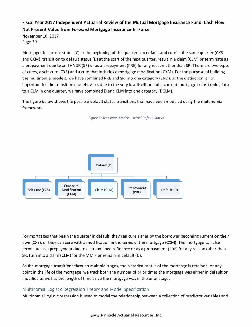
The figure below shows the possible default status transitions that have been modeled using the multinomial
framework.
Figure 5: Transition Models – Initial Default Status
For mortgages that begin the quarter in default, they can cure either by the borrower becoming current on their
own (CXS), or they can cure with a modification in the terms of the mortgage (CXM). The mortgage can also
terminate as a prepayment due to a streamlined refinance or as a prepayment (PRE) for any reason other than
SR, turn into a claim (CLM) for the MMIF or remain in default (D).
As the mortgage transitions through multiple stages, the historical status of the mortgage is retained. At any
point in the life of the mortgage, we track both the number of prior times the mortgage was either in default or
modified as well as the length of time since the mortgage was in the prior stage.
Multinomial Logistic Regression Theory and Model Specification
Multinomial logistic regression is used to model the relationship between a collection of predictor variables and
Default (D)
Self Cure (CXS)Cure with
Modification (CXM)
Claim (CLM)Prepayment
(PRE)Default (D)

Fiscal Year 2017 Independent Actuarial Review of the Mutual Mortgage Insurance Fund: Cash Flow
Net Present Value from Forward Mortgage Insurance‐In‐Force
November 10, 2017 Page 40
Pinnacle Actuarial Resources, Inc.
the distributional behavior of a polytomous response variable. It is a likelihood‐based methodology and may be
viewed as the generalization of logistic regression for a response variable with more than two levels.
To formalize its description, let the response variable Y take m possible levels, denoted for simplicity as 1,…,m,
and assume there is a collection of g predictors X ,…, X , that is used to model Y’s distribution. We assume that
Y and X ,…, X are jointly observed n times with the ith random observation being labeled as
Y , X ,…, X and its realized value y , x ,…, x .
In a multinomial logistic regression, the mathematical structure of the model is set by the following two
assumptions:
1. The g+1 length random vectors <Y , X ,…, X > are jointly independent across all i
2. Given that X ,…, X have been observed at x ,…, x , Y ’s distribution is assumed to be multinomial
with
P(Y = l) = exp( +∑ ∙x )/(∑ exp( +∑ ∙x )) ,
where the are unknown regression parameters and the j are unknown intercept parameters. [Note:
To prevent over‐specification of the model due to the constraint that the above probabilities sum to 1
over l=1,…,m, a base level j is chosen such that and are set equal to zero.] Thus, if j = 1, then
P(Y =1) = 1/(1 ∑ exp( +∑ ∙x )) .
It now follows the likelihood equation for this model is given by
∏ P(Y =y ) = ∏ exp( +∑ ∙x )/(∑ exp( +∑ ∙x )).
The multinomial logistic regression procedure optimizes the above likelihood over the unknown parameters in
order to find those parameters that are most likely to have given rise to the data.
The target variables for the current and default transition models are shown above in Figure 4 and Figure 5. The
independent variables used in the models are described in the following section. Twelve models were built, six
for the current (C) transitions and six for the Default (D) transitions. Three products are modeled: fixed rate 30‐
year term, fixed rate 15‐year term and adjustable rate mortgages. Each of the three products are further sub‐
divided if they are a result of SR. The model development was completed using a train/validate approach. A
random sample of the data is used to train the multinomial model, to determine inclusion and exclusion of
explanatory variables, and to calculate model parameters. The remaining sample, the validation data, is used as
a final validation step to test the predictive power of the final model.
To generate the random sample, random numbers were added to the dataset at the case level using a random
number generator. The random numbers were drawn from a uniform distribution between 0 and 1. Based on

Fiscal Year 2017 Independent Actuarial Review of the Mutual Mortgage Insurance Fund: Cash Flow
Net Present Value from Forward Mortgage Insurance‐In‐Force
November 10, 2017 Page 41
Pinnacle Actuarial Resources, Inc.
these random numbers, 70% of the cases were assigned to the train dataset, and 30% were assigned to the
validation dataset.
There are approximately 33 million single‐family mortgages insured by FHA originated between the first quarter
of fiscal year 1975 and the third quarter of fiscal year 2017. Sampling enhances the efficiency of model
estimation. In predictive modeling, a choice‐based sample is commonly used for large populations with
relatively rare events of interest. We use a sampling process for estimating the transition equations where the
sampling rates are determined by the ending condition of each mortgage at each period.
For the transition models with the initial condition of C, we sample ending conditions using the following
sampling percentages:
Table 16: Current Transition Model Sampling Percentages
Ending Condition Sampling Percentage
Current (C) 2.5%
Current with Self‐Cure (CXS) 100%
Current with Mortgage Modification (CSM) 100%
Default/Claim (DCLM) 100%
Pre‐payment (PRE) 50%
Streamline Refinance (SR) 50%
For transition models with the initial condition of D, we sample 50% of the records with ending condition of D.
For all other ending conditions, we used 100% of the data.
Section 2: Transition Model Explanatory Variables
Multiple categories of explanatory variables were used in development of the transition models.
Fixed initial mortgage characteristics: market rate, initial mortgage size, spread at origination
Fixed initial borrower characteristics: down payment assistance, first‐time home buyer, credit score,
cohort year
Property characteristics: the number of living units, initial home values
Dynamic variables based on mortgage information: prior default indicator, prior mortgage modification,
LTV ratio, interest rate spread, TEI (expense to income ratio), mortgage period
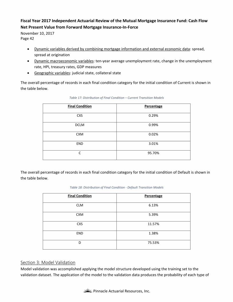
Fiscal Year 2017 Independent Actuarial Review of the Mutual Mortgage Insurance Fund: Cash Flow
Net Present Value from Forward Mortgage Insurance‐In‐Force
November 10, 2017 Page 42
Pinnacle Actuarial Resources, Inc.
Dynamic variables derived by combining mortgage information and external economic data: spread,
spread at origination
Dynamic macroeconomic variables: ten‐year average unemployment rate, change in the unemployment
rate, HPI, treasury rates, GDP measures
Geographic variables: judicial state, collateral state
The overall percentage of records in each final condition category for the initial condition of Current is shown in
the table below.
Table 17: Distribution of Final Condition – Current Transition Models
Final Condition Percentage
CXS 0.29%
DCLM 0.99%
CXM 0.02%
END 3.01%
C 95.70%
The overall percentage of records in each final condition category for the initial condition of Default is shown in
the table below.
Table 18: Distribution of Final Condition ‐ Default Transition Models
Final Condition Percentage
CLM 6.13%
CXM 5.39%
CXS 11.57%
END 1.38%
D 75.53%
Section 3: Model Validation
Model validation was accomplished applying the model structure developed using the training set to the
validation dataset. The application of the model to the validation data produces the probability of each type of

Fiscal Year 2017 Independent Actuarial Review of the Mutual Mortgage Insurance Fund: Cash Flow
Net Present Value from Forward Mortgage Insurance‐In‐Force
November 10, 2017 Page 43
Pinnacle Actuarial Resources, Inc.
transition. The actual target variable is then compared to the predicted target variable to ensure the model fits
the transition process without over‐fitting the actual data.
Specifically, for the final condition transition state, we calculate the actual transition rate and the predicted
transition rate. The actual transition is 1.0 for the final transition state of the record and 0.0 for all other
transition states. The probability of each final transition state for each record in the validation dataset is derived
from the model parameters. The sum of all predicted final condition transition states’ probabilities is 1.0 for
each record.
Decile charts are then created for each final condition transition state. All records are sorted, or ranked, in
increasing order by the predicted probability. Ten equal sized decile groups are created with 10% of the records
in each group. The sum of the actual probability and the sum of the predicted probability for each ending
condition within each decile is calculated. The total number of actual and predicted transitions are compared for
consistency. The objective of a model is to have a significant spread in predicted values while maintaining a close
relationship between the resulting actual and predicted values.
Current Transition Models
The validation chart for the ending condition of Current is shown below.
Figure 6: Current Transition Model Validation ‐ Ending Condition Current
The spread in prediction of the ending condition of Current has a range of roughly 10 to 1. In addition, the actual
and predicted ratio by decile for ending condition of Current are consistent.
The validation chart for the ending condition of Default/Claim is shown below.

Fiscal Year 2017 Independent Actuarial Review of the Mutual Mortgage Insurance Fund: Cash Flow
Net Present Value from Forward Mortgage Insurance‐In‐Force
November 10, 2017 Page 44
Pinnacle Actuarial Resources, Inc.
Figure 7: Current Transition Model Validation ‐ Ending Condition Default/Claim
The spread in prediction of the ending condition of Default/Claim has a range of approximately 13 to 1. In
addition, the actual and predicted ratio by decile for ending condition of Default/Claim are consistent.
The validation chart for the ending condition of Cure with Modification is shown below.
Figure 8: Current Transition Model Validation ‐ Ending Condition Cure with Modification

Fiscal Year 2017 Independent Actuarial Review of the Mutual Mortgage Insurance Fund: Cash Flow
Net Present Value from Forward Mortgage Insurance‐In‐Force
November 10, 2017 Page 45
Pinnacle Actuarial Resources, Inc.
The number of CXM ending conditions in the historical data is relatively small, so the validation results are
volatile. However, there is a significant spread in segmentation between deciles, and there is also a consistent
relationship between the actual and predicted transitions by decile.
The validation chart for the ending condition of Self‐Cure is shown below.
Figure 9: Current Transition Model Validation ‐ Ending Condition Self‐Cure
The spread in prediction of the ending condition of Self‐Cure has a range of approximately 100 to 1. In addition,
the actual and predicted ratio by decile for ending condition of Self‐Cure are consistent.
The validation chart for the ending condition of Refinance is shown below.

Fiscal Year 2017 Independent Actuarial Review of the Mutual Mortgage Insurance Fund: Cash Flow
Net Present Value from Forward Mortgage Insurance‐In‐Force
November 10, 2017 Page 46
Pinnacle Actuarial Resources, Inc.
Figure 10: Current Transition Model Validation ‐ Ending Condition Refinance
The spread in prediction of the ending condition of Refinance has a range of approximately 25 to 1. In addition,
the actual and predicted ratio by decile for ending condition of Refinance are consistent.
Default Transition Models
The validation chart for the ending condition of Default is shown below.

Fiscal Year 2017 Independent Actuarial Review of the Mutual Mortgage Insurance Fund: Cash Flow
Net Present Value from Forward Mortgage Insurance‐In‐Force
November 10, 2017 Page 47
Pinnacle Actuarial Resources, Inc.
Figure 11: Default Transition Model Validation ‐ Ending Condition Default
The spread in prediction of the ending condition of Default has a range of roughly 3 to 1. In addition, the actual
and predicted ratio by decile for ending condition of Default are consistent.
The validation chart for the ending condition of Claim is shown below.
Figure 12: Default Transition Model Validation ‐ Ending Condition Claim

Fiscal Year 2017 Independent Actuarial Review of the Mutual Mortgage Insurance Fund: Cash Flow
Net Present Value from Forward Mortgage Insurance‐In‐Force
November 10, 2017 Page 48
Pinnacle Actuarial Resources, Inc.
The spread in prediction of the ending condition of Claim has a range of approximately 20 to 1. In addition, the
actual and predicted ratio by decile for ending condition of Claim are consistent.
The validation chart for the ending condition of Cure with Modification is shown below.
Figure 13: Default Transition Model Validation ‐ Ending Condition Cure with Modification
The number of CXM ending conditions in the historical data is relatively small, so the validation results are
volatile. However, there is a significant spread in segmentation between deciles, and there is a consistent
relationship between the actual and predicted transitions by decile also.
The validation chart for the ending condition of Self‐Cure is shown below.

Fiscal Year 2017 Independent Actuarial Review of the Mutual Mortgage Insurance Fund: Cash Flow
Net Present Value from Forward Mortgage Insurance‐In‐Force
November 10, 2017 Page 49
Pinnacle Actuarial Resources, Inc.
Figure 14: Default Transition Model Validation ‐ Ending Condition Self‐Cure
The spread in prediction of the ending condition of Self‐Cure has a range of approximately 15 to 1. In addition,
the actual and predicted ratio by decile for ending condition of Self‐Cure are consistent.
The validation chart for the ending condition of Refinance is shown below.
Figure 15: Default Transition Model Validation ‐ Ending Condition Refinance

Fiscal Year 2017 Independent Actuarial Review of the Mutual Mortgage Insurance Fund: Cash Flow
Net Present Value from Forward Mortgage Insurance‐In‐Force
November 10, 2017 Page 50
Pinnacle Actuarial Resources, Inc.
The spread in prediction of the ending condition of Refinance has a range of approximately 22 to 1. In addition,
the actual and predicted ratio by decile for ending condition of Refinance are consistent.

Fiscal Year 2017 Independent Actuarial Review of the Mutual Mortgage Insurance Fund: Cash Flow
Net Present Value from Forward Mortgage Insurance‐In‐Force
November 10, 2017 Page 51
Pinnacle Actuarial Resources, Inc.
Appendix C: Loss Severity Models This appendix describes the loss severity models used in this analysis. One of the primary sources of variation in
the MMIF performance has been the loss severity experienced on mortgages that terminate as claims. In the
case of a single mortgage, net loss is defined as the difference between the acquisition cost to HUD
(acq_cost_to_HUD) from the IDB table and the recoveries realized by FHA on properties owned. We predict the
net loss by modeling the probability of the type of claim that develops, modeling separately the loss for each
type of claim and the recovery for REO claims.
In this appendix, we also summarize the model specifications, describe the explanatory variables used and
provide validation exhibits for the final models.
Model Specifications
Typically, when an FHA‐endorsed mortgage terminates as a claim, the property is conveyed to FHA, and FHA
makes a payment to the lender to settle the claim and acquire the underlying property. That is, the underlying
house becomes real estate owned, or REO. The claim payment FHA makes to the servicer, known as the
acquisition cost, consists of three components:
1. the outstanding unpaid principal balance on the mortgage;
2. the foregone interest advanced by the servicer as a result of the mortgage default; and
3. legal and administrative costs paid by the servicer associated with foreclosure, including any expenses
associated with the cost of repairing or maintaining the property prior to conveyance.
The formula for acquisition cost is:
Acquisition Cost = Unpaid Principal Balance + Foregone Interest + Foreclosure Expense
Following acquisition, FHA attempts to sell the property, sometimes at a reduced price in order to assist low‐
income prospective homebuyers in achieving homeownership. During the period when the property is held by
FHA, but not yet sold, FHA incurs various holding costs associated with maintenance, repairs, tax payments and
expenses incurred in preparing the property for sale. Upon sale of the collateral property, FHA receives the sale
price less any sales expenses. In sum, the net loss amount is the net amount that FHA cannot recoup from this
process:
Net Loss = Acquisition Cost + Holding Cost ‐ Sale Price + Sale Expense
Table 19 shows the distribution of different types of FHA claim terminations. Conveyance refers to the
foreclosure procedure discussed above, wherein the property is conveyed to FHA after foreclosure is completed.
This is the most common type of claim.
FHA permits pre‐foreclosure sales (PFS) as an alternative to the foreclosure process. In the case of a PFS, the
property is sold by the borrower without the foreclosure process being completed, or even started in some
cases. Instead of acquiring the foreclosed house, FHA directly pays the loss amount claimed by the lender. The

Fiscal Year 2017 Independent Actuarial Review of the Mutual Mortgage Insurance Fund: Cash Flow
Net Present Value from Forward Mortgage Insurance‐In‐Force
November 10, 2017 Page 52
Pinnacle Actuarial Resources, Inc.
loss amount of a PFS case is reported as an acquisition cost to FHA. By 2012, the percentage of PFS was just
under 24%. Since then, the percentage of PFS has decreased to under 9%.
There was a significant volume of note (non‐performing mortgage) sales from fiscal year 2003 through fiscal
year 2006. From fiscal year 2007 to fiscal year 2012, there were few note sales. By 2014, however, the
percentage of note sales rose above 27%. In these cases, the expenses of foreclosure procedures and
subsequent house sales are avoided by FHA. Note sales are discretionary and highly unpredictable. For
forecasting purposes, we use a note sale override to incorporate recent note sale transactions. We do not model
note sales as a continuing program.
FHA changed its servicing guide in 2013 to allow foreclosure without conveyance. This consists of a TPS during
the foreclosure auction. A third party, instead of FHA, acquires the property directly from the foreclosure
auction. This process allows FHA to avoid the process and expenses of property disposition after conveyance
including any associated holding costs.
Table 19: Percentage of Claim Termination Types by Fiscal Claim Year
Table 20 shows the average net loss for the combined foreclosure (REO and TPS) and PFS claims by claim fiscal
year for 1991 to 2017. The average net loss increased from 1991 to 2012, reaching a high of almost $129,000 in
fiscal year 2012. Since 2012, the average net loss has decreased.
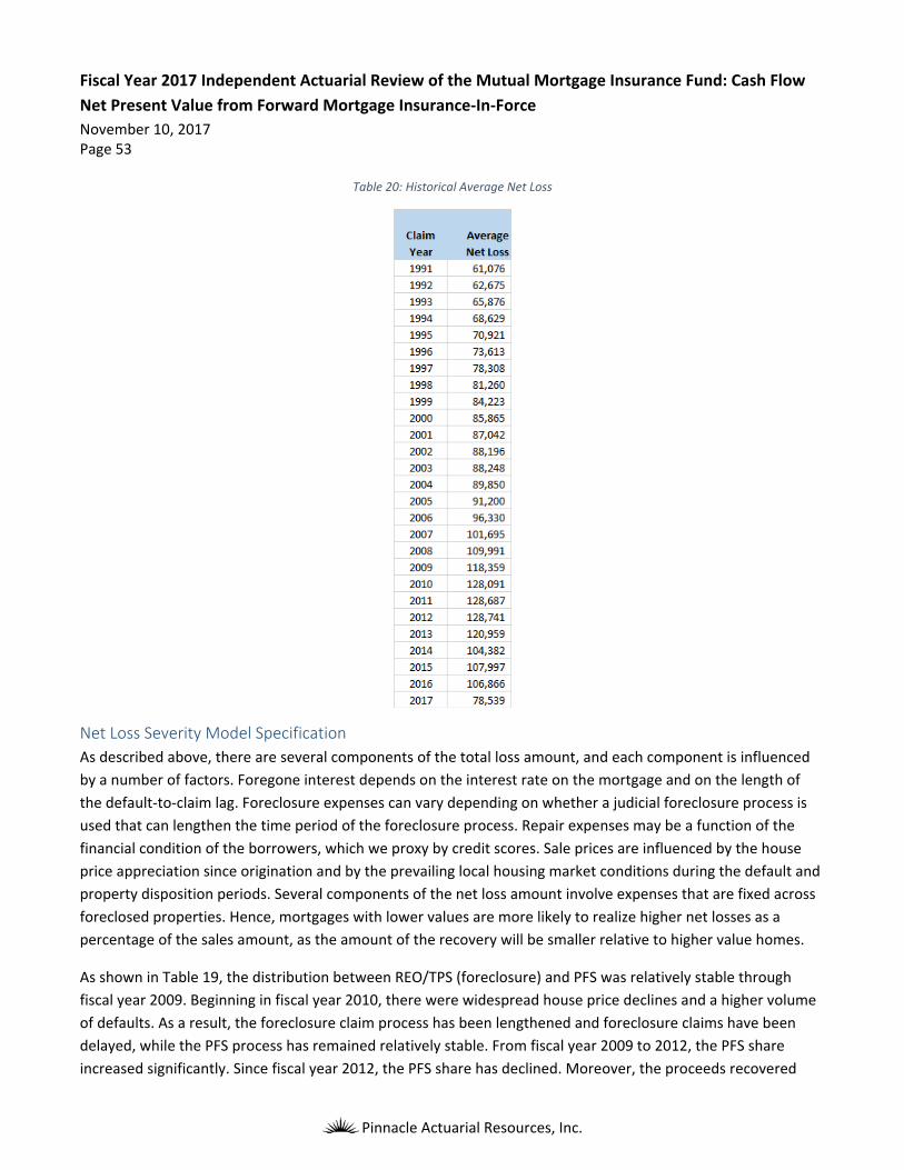
Fiscal Year 2017 Independent Actuarial Review of the Mutual Mortgage Insurance Fund: Cash Flow
Net Present Value from Forward Mortgage Insurance‐In‐Force
November 10, 2017 Page 53
Pinnacle Actuarial Resources, Inc.
Table 20: Historical Average Net Loss
Net Loss Severity Model Specification
As described above, there are several components of the total loss amount, and each component is influenced
by a number of factors. Foregone interest depends on the interest rate on the mortgage and on the length of
the default‐to‐claim lag. Foreclosure expenses can vary depending on whether a judicial foreclosure process is
used that can lengthen the time period of the foreclosure process. Repair expenses may be a function of the
financial condition of the borrowers, which we proxy by credit scores. Sale prices are influenced by the house
price appreciation since origination and by the prevailing local housing market conditions during the default and
property disposition periods. Several components of the net loss amount involve expenses that are fixed across
foreclosed properties. Hence, mortgages with lower values are more likely to realize higher net losses as a
percentage of the sales amount, as the amount of the recovery will be smaller relative to higher value homes.
As shown in Table 19, the distribution between REO/TPS (foreclosure) and PFS was relatively stable through
fiscal year 2009. Beginning in fiscal year 2010, there were widespread house price declines and a higher volume
of defaults. As a result, the foreclosure claim process has been lengthened and foreclosure claims have been
delayed, while the PFS process has remained relatively stable. From fiscal year 2009 to 2012, the PFS share
increased significantly. Since fiscal year 2012, the PFS share has declined. Moreover, the proceeds recovered

Fiscal Year 2017 Independent Actuarial Review of the Mutual Mortgage Insurance Fund: Cash Flow
Net Present Value from Forward Mortgage Insurance‐In‐Force
November 10, 2017 Page 54
Pinnacle Actuarial Resources, Inc.
from REO and PFS sales differ significantly. To achieve more accurate estimates of net loss severities, we
adopted a three‐stage model:
1. Model to predict the development of an REO, TPS or PFS claims
2. Model of gross loss severity conditional on claim being an REO, TPS or PFS claim
3. Model of recovery amount conditional on claim being a foreclosure REO claim
The net loss severity model follows the flowchart in Figure 16.
Figure 16: Net Loss Severity Model
First, we estimate the probability that a claim is settled by the REO, TPS, or PFS process. To model the first‐stage
choice event, we used a multinomial logistic model to estimate the probability of the claim settlement type.
Second, we estimate the gross loss severity as a function of all the same explanatory factors used in the
multinomial model. The gross loss severity distribution is smooth and continuous with a long right tail. Thus, we
use a GLM approach with a Gamma error structure and a log link function to develop the gross loss severity
models. The Gamma structure is used for each gross loss severity model (REO, TPS, PFS). For REO claims, a
recovery model estimating sales proceeds net of the Capital Income Expenses is built using a similar framework.
In addition to the loss severity models described above, we also developed a set of models to project loss
mitigation costs. Implemented in 1996, the loss mitigation program was designed as a way to help financially
stressed borrowers stay in their homes. Loss mitigation costs can be incurred from modifying the terms of the
mortgage, allowing a borrower to refinance into a new mortgage and writing off a portion of the unpaid
principal (partial claim), or a forbearance, which is a written agreement with the borrower which includes a plan
Claim
REO
Net Loss ‐REO
TPS
Net Loss ‐TPS
PFS
Net Loss ‐PFS
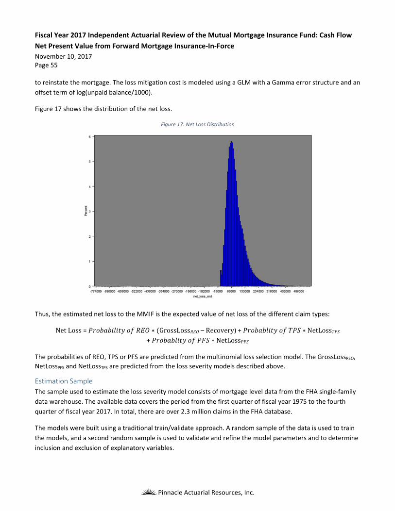
Fiscal Year 2017 Independent Actuarial Review of the Mutual Mortgage Insurance Fund: Cash Flow
Net Present Value from Forward Mortgage Insurance‐In‐Force
November 10, 2017 Page 55
Pinnacle Actuarial Resources, Inc.
to reinstate the mortgage. The loss mitigation cost is modeled using a GLM with a Gamma error structure and an
offset term of log(unpaid balance/1000).
Figure 17 shows the distribution of the net loss.
Figure 17: Net Loss Distribution
Thus, the estimated net loss to the MMIF is the expected value of net loss of the different claim types:
NetLoss = ∗ GrossLoss – Recovery) + ∗ NetLoss
+ ∗ NetLoss
The probabilities of REO, TPS or PFS are predicted from the multinomial loss selection model. The GrossLossREO,
NetLossPFS and NetLossTPS are predicted from the loss severity models described above.
Estimation Sample
The sample used to estimate the loss severity model consists of mortgage level data from the FHA single‐family
data warehouse. The available data covers the period from the first quarter of fiscal year 1975 to the fourth
quarter of fiscal year 2017. In total, there are over 2.3 million claims in the FHA database.
The models were built using a traditional train/validate approach. A random sample of the data is used to train
the models, and a second random sample is used to validate and refine the model parameters and to determine
inclusion and exclusion of explanatory variables.

Fiscal Year 2017 Independent Actuarial Review of the Mutual Mortgage Insurance Fund: Cash Flow
Net Present Value from Forward Mortgage Insurance‐In‐Force
November 10, 2017 Page 56
Pinnacle Actuarial Resources, Inc.
Explanatory Variables
Multiple categories of explanatory variables were used.
Fixed initial mortgage characteristics: ARM adjustment period, mortgage product, interest rate, initial
mortgage size, spread at origination
Fixed initial borrower characteristics: down payment assistance, first time home buyer, credit score
Property characteristics: the number of living units, initial home values
Dynamic variables based on mortgage information: prior default indicator, prior mortgage modification,
LTV ratio, interest rate spread, TEI, age of mortgage
Dynamic variables derived by combining mortgage information and external economic data: spread,
spread at origination
Dynamic macroeconomic variables: 10‐year average unemployment rate, change in the unemployment
rate, prior year unemployment rate, HPI, state unemployment rate relative to countrywide
unemployment rate, CMT rates, state unemployment rate
Geographic variables: Judicial state, collateral state
The explanatory variables used in the loss severity model are the same as those used in the mortgage status
transition models.
Model Validation
Model validation was accomplished by applying the models developed using the training set to the validation
dataset. The application of the models to the validation data produces the probability of each type of claim
settlement type and a predicted net loss. The actual target variable is then compared to the predicted target
variable to ensure the model fits the claim settlement process and net loss process without over‐fitting the
actual data.
Specifically for the loss settlement models, for the final loss settlement type we calculate the predicted
probability of the settlement type. The actual settlement type is 1.0 for the final type of claim and 0.0 for all
other claim types. The probability of each claim type for each record in the validation dataset is derived from the
model parameters. The sum of all predicted claim type probabilities is 1.0 for each record.
For the net loss severity models, we calculate a predicted net loss. We also summarize the actual net loss for
each claim. The predicted loss severity for each record in the validation dataset is derived from the model
parameters.
Decile charts are then created for each final claim type selection and each net loss. All records are sorted, or
ranked, in ascending order by the predicted value. Ten equal‐sized decile groups are created with 10% of the
records in each group. The sum of the actual probability and the sum of the predicted probability for each claim
type within each decile is calculated for the claim type models. The sum of the actual net loss and the sum of the
predicted net loss within each decile is calculated for the loss severity models. The actual and predicted
numbers are then compared for consistency. The objective of a model is to have a significant spread in predicted
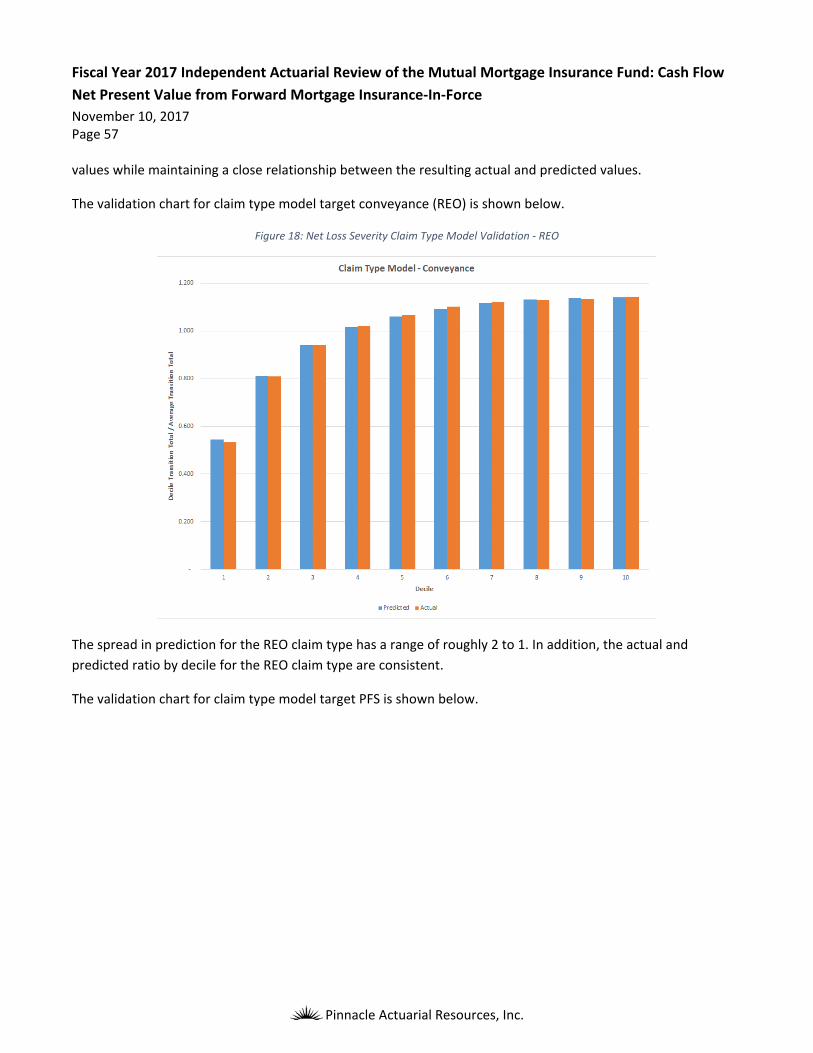
Fiscal Year 2017 Independent Actuarial Review of the Mutual Mortgage Insurance Fund: Cash Flow
Net Present Value from Forward Mortgage Insurance‐In‐Force
November 10, 2017 Page 57
Pinnacle Actuarial Resources, Inc.
values while maintaining a close relationship between the resulting actual and predicted values.
The validation chart for claim type model target conveyance (REO) is shown below.
Figure 18: Net Loss Severity Claim Type Model Validation ‐ REO
The spread in prediction for the REO claim type has a range of roughly 2 to 1. In addition, the actual and
predicted ratio by decile for the REO claim type are consistent.
The validation chart for claim type model target PFS is shown below.

Fiscal Year 2017 Independent Actuarial Review of the Mutual Mortgage Insurance Fund: Cash Flow
Net Present Value from Forward Mortgage Insurance‐In‐Force
November 10, 2017 Page 58
Pinnacle Actuarial Resources, Inc.
Figure 19: Net Loss Severity Claim Type Model Validation ‐ PFS
The number of PFS claims are limited, and therefore the validation exhibits are volatile. However, the spread in
prediction for the PFS claim type is significant, and the actual and predicted ratio by decile for the PFS claim type
are consistent.
The validation chart for claim type model target TPS is shown below.

Fiscal Year 2017 Independent Actuarial Review of the Mutual Mortgage Insurance Fund: Cash Flow
Net Present Value from Forward Mortgage Insurance‐In‐Force
November 10, 2017 Page 59
Pinnacle Actuarial Resources, Inc.
Figure 20: Net Loss Severity Claim Type Model Validation ‐ TPS
The spread in prediction for the TPS claim type has a significant range. In addition, the actual and predicted ratio
by decile for the REO claim type are consistent.
The validation chart for the REO gross loss severity model is shown below.
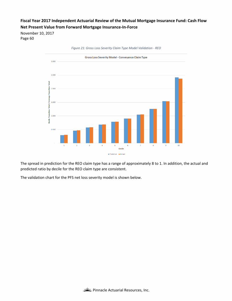
Fiscal Year 2017 Independent Actuarial Review of the Mutual Mortgage Insurance Fund: Cash Flow
Net Present Value from Forward Mortgage Insurance‐In‐Force
November 10, 2017 Page 60
Pinnacle Actuarial Resources, Inc.
Figure 21: Gross Loss Severity Claim Type Model Validation ‐ REO
The spread in prediction for the REO claim type has a range of approximately 8 to 1. In addition, the actual and
predicted ratio by decile for the REO claim type are consistent.
The validation chart for the PFS net loss severity model is shown below.

Fiscal Year 2017 Independent Actuarial Review of the Mutual Mortgage Insurance Fund: Cash Flow
Net Present Value from Forward Mortgage Insurance‐In‐Force
November 10, 2017 Page 61
Pinnacle Actuarial Resources, Inc.
Figure 22: Net Loss Severity Claim Type Model Validation ‐ PFS
The spread in prediction for the PFS claim type has a range of approximately 6 to 1. In addition, the actual and
predicted ratio by decile for the REO claim type are consistent.
The validation chart for the TPS net loss severity model is shown below.

Fiscal Year 2017 Independent Actuarial Review of the Mutual Mortgage Insurance Fund: Cash Flow
Net Present Value from Forward Mortgage Insurance‐In‐Force
November 10, 2017 Page 62
Pinnacle Actuarial Resources, Inc.
Figure 23: Net Loss Severity Claim Type Model Validation ‐ TPS
The spread in prediction for the PFS claim type has a range of approximately 10 to 1. In addition, the actual and
predicted ratio by decile for the REO claim type are consistent.

Fiscal Year 2017 Independent Actuarial Review of the Mutual Mortgage Insurance Fund: Cash Flow
Net Present Value from Forward Mortgage Insurance‐In‐Force
November 10, 2017 Page 63
Pinnacle Actuarial Resources, Inc.
Appendix D: Economic Scenarios To measure the possible variation in MMIF’s Cash Flow NPV on the existing portfolio, we developed a baseline
projection using OMB Economic Assumptions and also projections for nine additional deterministic economic
scenarios from Moody’s. For this analysis, we used the Moody’s September 2017 forecast of the U.S. economy.
For purposes of our analysis, the components of Moody’s forecast include:
HPI at the MSA, state, regional and national levels
1‐year CMT rate
10‐year CMT rate
Commitment rate on 30‐year fixed‐rate mortgages
Unemployment rates at the MSA, state, regional and national levels
GDP
A summary of a portion of the economic data used in the OMB simulation is presented in Table 21. We used a
quarterly frequency and local HPI and unemployment rate in deriving the Cash Flow NPV. The quarterly
economic factors forecasted by Moody’s are available from fiscal years 2017 through 2047.
Table 21: Summary of OMB Economic Assumptions
Source: OMB Economic Assumptions for the 2018 Fall Budget Baseline, March 2017
Alternative Scenarios
To assess the effect of alternative economic scenarios on the Cash Flow NPV, nine alternative scenarios from
Moody’s were used. The nine Moody’s scenarios are:
Baseline
Stronger Near‐Term Growth
Slower Near‐Term Growth
Moderate Recession
Fiscal
Year
FHFA Purchase‐
Only Home Index
FHLMC Contract
Rate on
Conventional
Mortgage
Commitments
1‐Year
Treasury
Rate (%)
10‐Year
Treasury
Rate (%)
National
Unemployment
Rate (%)
2017 242.10 4.44 1.16 2.66 4.6
2018 252.52 5.19 1.94 3.28 4.4
2019 261.51 5.45 2.47 3.44 4.6
2020 269.36 5.85 3.01 3.78 4.7
2021 277.44 5.94 3.24 3.81 4.8
2022 285.21 6.00 3.33 3.83 4.8
2023 292.25 6.04 3.37 3.84 4.8
2024 299.45 6.06 3.39 3.84 4.8
2025 306.83 6.08 3.39 3.84 4.8
2026 314.50 6.09 3.39 3.84 4.8
2027 322.57 6.10 3.39 3.84 4.8

Fiscal Year 2017 Independent Actuarial Review of the Mutual Mortgage Insurance Fund: Cash Flow
Net Present Value from Forward Mortgage Insurance‐In‐Force
November 10, 2017 Page 64
Pinnacle Actuarial Resources, Inc.
Protracted Slump
Below‐Trend Long‐Term Growth
Stagflation
Next‐Cycle Recession
Low Oil Price
The Moody’s projections provide a range of better than expected economic assumptions and worse than
expected economic assumptions. This range of assumptions produces a range of Cash Flow NPV projections.
Graphical Depiction of the Scenarios
Figure 24 shows the future movements of the HPI under the baseline and the alternative economic scenarios.
For the OMB projections, the HPI increases as a fairly steady rate throughout the entire projection period. For
the Moody’s Baseline Scenario, the HPI appreciation rate increases at a slower rate through 2022, at which time
the rate of increase becomes greater than the OMB rate. The Moody’s Baseline HPI projection is higher than the
OMB baseline after 2024.
Figure 24: Paths of the Future National House Price Index in Different Scenarios

Fiscal Year 2017 Independent Actuarial Review of the Mutual Mortgage Insurance Fund: Cash Flow
Net Present Value from Forward Mortgage Insurance‐In‐Force
November 10, 2017 Page 65
Pinnacle Actuarial Resources, Inc.
Figure 25 shows the forecasted mortgage rate of 30‐year fixed‐rate mortgages for the nine scenarios. OMB’s
forecast shows that the rate will rise steadily over the projection period to just over 6% by 2027. Moody’s
Baseline forecast for the 30‐year fixed interest rate shows that the mortgage interest rate increases to just over
5.6% by 2020, and then hovers around a long‐term average rate of around 5.5%. The OMB projection is a
composite interest rate projection, whereas the Moody’s projections are separate by mortgage product.
Therefore, the trends in projection can be compared but the absolute value of the projected mortgage rates are
not directly comparable. For the Moody’s projections, we use the 30‐year fixed rate as this represents the
majority of the mortgage products sold.
Figure 25: Paths of the Future Mortgage Rate
Figure 26 shows the forecasted unemployment rate under alternative economic scenarios. OMB projects the
unemployment rate to essentially remain constant over the projection period, decreasing slightly to 4.4% by
2018 and then rising to 4.8%. The Moody’s Baseline forecast projects that the unemployment rate will decrease
to under 4% in 2019, and then increases to a long‐term average of just over 5%.

Fiscal Year 2017 Independent Actuarial Review of the Mutual Mortgage Insurance Fund: Cash Flow
Net Present Value from Forward Mortgage Insurance‐In‐Force
November 10, 2017 Page 66
Pinnacle Actuarial Resources, Inc.
Figure 26: Paths of Future National Unemployment Rate
Stochastic Simulations
This section describes the stochastic models which were fit to generate the economic variable simulations used
in the analysis of the Forward Mortgage Portfolio.
The modeled economic variables include:
1‐Year CMT Rates
3‐Month CMT Rates
6‐Month CMT Rates
2‐Year CMT Rates
3‐Year CMT Rates
5‐Year CMT Rates
7‐Year CMT Rates
10‐Year CMT Rates
20‐Year CMT Rates

Fiscal Year 2017 Independent Actuarial Review of the Mutual Mortgage Insurance Fund: Cash Flow
Net Present Value from Forward Mortgage Insurance‐In‐Force
November 10, 2017 Page 67
Pinnacle Actuarial Resources, Inc.
30‐Year CMT Rates
30‐Year FRM Rates
FHFA National Purchase Only House Price Index (HPI‐PO)
Unemployment Rates
GDP
Historical Data
A. Interest Rates
Figure 27 shows historical interest rates since the first quarter of 1971.
This graph illustrates the variability of interest rates over time and the consistent spread between rates. Shown
are the 1‐year CMT rate (tr1y), 10‐year CMT rate (tr10y) and the 30‐year FRM rate (mr).
High inflation rates caused by the global oil crisis in the late 1970’s were the major cause for the historically high
level of interest rates in early 1980’s. The Federal Reserve shifted its monetary policy from managing interest
rates to managing the money supply as a way to influence interest rates after this period of time. The 1‐year
CMT rate was around 5% in calendar year (CY) 1971 and increased steadily to its peak of 16.31% in the third
quarter of CY 1981. Subsequently, the 1‐year CMT rate followed a decreasing trend and reached an all‐time low
of 0.10% in the second quarter of 2014. Since then, rates have started a slow upward trend.
Figure 27: Historical Interest Rates (%)
Figure 28 shows historical interest rate spreads, including the spread between 10‐year and 1‐year CMT rates
(tr10y_s) and the spread between the 30‐year mortgage rate and the 10‐year CMT rate (mr10y_s). Both spreads

Fiscal Year 2017 Independent Actuarial Review of the Mutual Mortgage Insurance Fund: Cash Flow
Net Present Value from Forward Mortgage Insurance‐In‐Force
November 10, 2017 Page 68
Pinnacle Actuarial Resources, Inc.
have positive values for most of the historical periods with long cycles. Small positive and negative spreads
typically correspond with economic downturns, such as those that occurred during the late 1970’s through early
1980’s. The spread of the mortgage rate over the 10‐year CMT rate is always positive, reflecting the premium for
credit risk.
Figure 28: Historical Interest Rate Spreads (%)
B. House Price Appreciation Rates
The national HPA rate is derived from the FHFA repeat sales HPI of purchase‐only (PO) transactions. The PO HPI
provides a reliable measure of housing market conditions, since it is based on repeat sales at market prices and
does not use any appraised values.
The HPA series being modeled is defined as:
ln (1)
Figure 29 shows the national quarterly HPA from CY 1971 Q1 to CY 2016 Q4. The long‐term average quarterly
HPA is approximately 0.83% (an annual rate of 3.30%).

Fiscal Year 2017 Independent Actuarial Review of the Mutual Mortgage Insurance Fund: Cash Flow
Net Present Value from Forward Mortgage Insurance‐In‐Force
November 10, 2017 Page 69
Pinnacle Actuarial Resources, Inc.
Figure 29: Historical Quarterly HPA
The HPA increased steadily before 2004, and the quarterly appreciation rate was around 1.13%. Subsequently,
house prices rose sharply starting in 2004. The average quarterly house price appreciation rate was 1.87% during
the subprime mortgage expansion period from 2004 to 2006, and reached its peak of 2.59% in the second
quarter of CY 2005. After 2006, the average growth rate of house price became negative until 2011, when
appreciation returned to a positive value. Table 22 shows the quarterly HPA by selected historical time periods.
Table 22: Average Quarterly HPA by Time Span
Period Average Quarterly HPA
1991 – 2003 1.13%
2004 – 2006 1.87%
2007 – 2010 ‐1.23%
2011 – 2017 1.03%

Fiscal Year 2017 Independent Actuarial Review of the Mutual Mortgage Insurance Fund: Cash Flow
Net Present Value from Forward Mortgage Insurance‐In‐Force
November 10, 2017 Page 70
Pinnacle Actuarial Resources, Inc.
Modeling Techniques
The primary modeling techniques used in developing the stochastic simulations include:
Auto Regressive Moving Average (ARMA)
General Auto Regressive Conditional Heteroscedasticity (GARCH)
ARMA models are typically specified as ARMA(p,q) where p is the auto regressive component of the series, and q
the moving average.
GARCH models are typically specified as GARCH(p,q) where p is the auto regressive component of , and q the
AR component of the error term.
Description and examples of using an ARMA‐GARCH model for time series analysis can be found in Engle and
Mezrich (1995)3.
1‐Year CMT Rate
In this section, we present historical statistics for the 1‐year CMT rate, describe the estimation model for the
stochastic process, and finally report the parameter estimates and their standard errors.
Table 23 shows the summary statistics of the historical 1‐year CMT rates for two time periods, one from 1971 to
current and the other from 1992 to current, as well as the simulated series. We can see that in the last 25 years,
interest rates have been much more stable than in the past.
Table 23: Statistics for the 1‐Year CMT Rates
Statistics Since 1971 Since 1992 Simulations
Mean 5.34% 2.69% 5.13%
Standard Deviation 3.64% 2.27% 2.37%
Max 16.31% 6.71% 28.21%
95th Percentile 11.83% 5.94% 12.31%
90th Percentile 10.02% 5.66% 10.31%
50th Percentile 5.44% 2.12% 4.24%
25th Percentile 2.30% 0.36% 2.05%
10th Percentile 0.27% 0.15% 1.13%
5th Percentile 0.15% 0.12% 0.81%
Minimum 0.10% 0.10% 0.01%
3 Engle, R. F. and J. Mezrich (1995), “Grappling with GARCH”, Risk Magazine, 8 (9), 112 – 17.

Fiscal Year 2017 Independent Actuarial Review of the Mutual Mortgage Insurance Fund: Cash Flow
Net Present Value from Forward Mortgage Insurance‐In‐Force
November 10, 2017 Page 71
Pinnacle Actuarial Resources, Inc.
An ARMA(2,4) parameterization was used to model the 1‐Year CMT rate (r1) difference from the previous
period. The model was estimated using data from the first quarter of CY 1971 to the third quarter of CY 2017.
The process takes the following form:
, , , , , , , (2)
Z1 is an independent Wiener random process with distribution N(0,1), and the variance (σ) of the residual term
follows a GARCH(1,1) process:
(3)
ε is the error term, which equals from equation (2).
The Full information maximum likelihood (FIML) method was used to estimate the parameters in equations (2)
and (3). The results are presented in Table 24.
Table 24: Estimation Results for 1‐Year CMT Rate Model
Parameter Estimate Std Dev t‐value prob>t µ 0.0003 0.0002 1.4052 0.1600 x1 0.0424 1.5880 0.0267 0.9787 x2 0.3361 1.3910 0.2416 0.8091 x3 0.3517 1.5558 0.2261 0.8212 x4 ‐0.4119 0.7487 ‐0.5502 0.5822 x4 0.1358 0.4423 0.3070 0.7589 x5 0.3051 0.3723 0.8195 0.4125
β0 0.0000 0.0000 0.0110 0.9912 β1 0.3094 0.0512 6.0382 0.0000 β2 0.6896 0.0424 16.2677 0.0000
Pearson’s GOF 0.9380
The model based on these parameters is used to simulate the 1‐year CMT rates for the forecast period starting
in the fourth quarter of FY 2017. The model fit was evaluated using Akaike Information Criterion (AIC) and
Pearson’s goodness‐of‐fit test.
A lower bound of 0.01 percent was applied to the simulated future 1‐year CMT rates to avoid negative rates in
the simulation.

Fiscal Year 2017 Independent Actuarial Review of the Mutual Mortgage Insurance Fund: Cash Flow
Net Present Value from Forward Mortgage Insurance‐In‐Force
November 10, 2017 Page 72
Pinnacle Actuarial Resources, Inc.
Additional Interest Rate Models
Additional models were developed to simulate the other interest rates. All models were estimated as a spread (difference) between the current maturity length and prior. Table 25 describes these spreads and models.
Table 25: Model Specification for Additional Interest Rates
Variable Variable Transformation Model Specification Notes
3‐month AR(1)‐GARCH(1,1)
6‐month ARMA(3,1)‐ARCH(1)
1‐year ARMA(2,4)‐GARCH(1,1) Base Interest Rate
2‐year AR(1)‐ARCH(1)
3‐year ARMA(2,1)‐ARCH(1)
5‐year ARMA(2,1)‐ARCH(1)
7‐year ARMA(2,1)‐ARCH(1)
10‐year ARMA(2,1)‐ARCH(1)
20‐year AR(2) dataset for 1980 forward did
not produce a statistically
significant model
30‐year ARMA(1,1)‐GARCH(1,1) used 10 year rate for spread
30‐year FRM AR(1)‐ARCH(1)
All models used AIC and/or Pearson’s goodness‐of‐fit test to determine the best fitting model. A lower bound of
0.01% was applied to the simulated future Treasury rates to avoid negative rates in the simulation. Figure 30
shows the projected interest rate values from a sample simulation.

Fiscal Year 2017 Independent Actuarial Review of the Mutual Mortgage Insurance Fund: Cash Flow
Net Present Value from Forward Mortgage Insurance‐In‐Force
November 10, 2017 Page 73
Pinnacle Actuarial Resources, Inc.
Figure 30: Interest Rate Sample Simulation
HPA
A. National HPA
The national HPA series was fit using as an ARMA(1,1)‐GARCH(1,1). The 1‐year CMT, 10‐year CMT, and mortgage
rates at time t and t‐1 were also included as external regressors in the following model formula:
, , , , ,
(4)
Z1 is an independent Wiener random process with distribution N(0,1), and the variance (σ) of the residual term
follows a GARCH(1,1) process:
(5)
The model specification and variable inclusions were determined by achieving appropriate coefficient signs and
significance, and overall model fit. FIML was used to estimate parameters in equations (4) and (5). The results
are shown in Table 26.

Fiscal Year 2017 Independent Actuarial Review of the Mutual Mortgage Insurance Fund: Cash Flow
Net Present Value from Forward Mortgage Insurance‐In‐Force
November 10, 2017 Page 74
Pinnacle Actuarial Resources, Inc.
Table 26: Estimation Results for the National HPA Model
Parameter Estimate Std Dev t‐value prob>t µ 0.0369 0.0070 5.3041 0.0000 x1 0.9552 0.0168 56.7543 0.0000 x2 ‐0.5776 0.0765 ‐7.5524 0.0000 x3 ‐0.4629 0.0867 ‐5.3379 0.0000 x4 0.2687 0.0858 3.1322 0.0017 x4 ‐0.5277 0.1804 ‐2.9248 0.0034 x5 0.1464 0.1378 1.0624 0.2880 x6 ‐0.6007 0.1463 ‐4.1058 0.0000 x7 0.2862 0.1405 2.0373 0.0416 x8 0.0369 0.0070 5.3041 0.0000 β0 0.0000 0.0000 0.6067 0.5441 β1 0.3277 0.1120 2.9262 0.0034 β2 0.6447 0.0754 8.5510 0.0000
Pearson’s GOF 0.9125
We used these parameters to simulate future HPAs from the first quarter of FY 2017.
B. Geographic dispersion
The MSA‐level HPA forecasts were based on Moody’s forecast of local and national HPA forecasts. Specifically, at
each time t, there is a dispersion of HPAs between the ith MSA or state level and the national forecast:
, , , (6)
This dispersion forecast under Moody’s base case was preserved for all local house price forecasts under
individual future economic paths. That is, for economic path j, the HPA of the ith MSA at time t was computed as:
, , , (7)
This approach retains the relative current housing market cycle among different geographic locations, and it
allows us to capture the geographical concentration of FHA’s current mortgage portfolio. This approach is also
consistent with Moody’s logic in creating local market HPA forecasts relative to the national HPA forecast under
alternative economic scenario forecasts.
We understand this approach is equivalent to assuming perfect correlation of dispersions among different
locations across simulated national HPA paths, which creates systematic house price decreases during economic
downturns and vice versa during booms. Due to Jensen’s Inequality, this tends to generate a more conservative
estimate of the Cash Flow NPV.

Fiscal Year 2017 Independent Actuarial Review of the Mutual Mortgage Insurance Fund: Cash Flow
Net Present Value from Forward Mortgage Insurance‐In‐Force
November 10, 2017 Page 75
Pinnacle Actuarial Resources, Inc.
Unemployment Rate
A. National Unemployment Rate
In our unemployment rate model, the unemployment rate depends on the prior unemployment rate, mortgage
rates and CMT rates.
We used quarterly data from CY 1971 through the first quarter of CY 2017 to estimate the national
unemployment rate. The model we adopted was:
(8)
where is the 1‐year CMT rate,
is the 30‐year mortgage rate to 10‐year CMT rate spread, and
is the unemployment rate auto regressive component.
The model specification and variable inclusions were determined by achieving appropriate coefficient signs and
significance, and overall model fit. FIML was used to estimate parameters in equation (8). The results are shown
in Table 27.
Table 27: Estimation Results for the National Unemployment Rate Model
Parameter Estimate Std Errorx1 0.0551 0.7039x2 0.021 ‐0.1273x3 0.0376 0.041
From the simulated interest rates and house prices, we applied the parameters shown in Table 27 to calculate
the corresponding national unemployment rate. Based on historical statistics, the national unemployment rate
was capped at 20% with a floor at 2%.
B. Geographic Dispersion
Following the same logic applied to the MSA‐level HPA forecasts, we first calculated the dispersion of
unemployment rates between the ith MSA or state level and the national level from Moody’s July base‐case
forecast at each time t:
, , , (9)
This dispersion forecast was preserved for all local unemployment rate forecasts under each individual future
economic path. That is, for economic path j, the unemployment rate of the ith MSA at time t was computed as:
, , , (10)

Fiscal Year 2017 Independent Actuarial Review of the Mutual Mortgage Insurance Fund: Cash Flow
Net Present Value from Forward Mortgage Insurance‐In‐Force
November 10, 2017 Page 76
Pinnacle Actuarial Resources, Inc.
For the simulation, we capped the unemployment rate at the local level at a maximum of 30% and a minimum of
1%.
Gross Domestic Product
For the GDP model, the GDP depends on the prior GDP, unemployment, mortgage and CMT rates.
We used quarterly data from CY 1971 through the first quarter of CY 2017 to estimate the national
unemployment rate. The model tested for integration, so first difference transformations were used prior to
estimations. The model adopted was an ARMA(1,1):
, (11)
where, is the 1‐year CMT rate,
, is the 30‐year mortgage rate to 10‐year CMT rate spread,
is the unemployment rate, and
is the unemployment rate auto regressive component.
The model specification and variable inclusions were determined by achieving appropriate coefficient signs and
significance, and overall model fit. FIML was used to estimate parameters in equation (6). The results are shown
in Table 28.
Table 28: Estimation Results for the National Gross Domestic Product Model
Parameter Estimate Std Errorx1 0.3878 0.0822x2 ‐0.9383 0.0371x3 1135.458 739.7173x4 ‐1298.61 899.3981x5 ‐12.5117 672.9905
Final Simulation Selection
A total of 1,000 simulation paths were generated using all of the economic variable models described to create a
large sample pool. From this pool, a random sample of 100 simulated series was drawn to be used for the Cash
Flow NPV stochastic simulations.

Fiscal Year 2017 Independent Actuarial Review of the Mutual Mortgage Insurance Fund: Cash Flow
Net Present Value from Forward Mortgage Insurance‐In‐Force
November 10, 2017 Page 77
Pinnacle Actuarial Resources, Inc.
Appendix E: Cash Flow Analysis
Introduction
The calculation of the Cash Flow NPV of the MMIF involves the estimation of the present value of future cash
flows generated by the existing portfolio. The analysis requires the projection of future prepayment and claim
incidences, and severity and cash flow items associated with each type of outcome. The Cash Flow NPV
represents future revenue and expenses associated with the existing book of mortgage guarantees. This
appendix describes the components of these cash flow calculations.
To develop the estimated Cash Flow NPV, our model incorporates projections of mortgage performance and
information about the existing portfolio composition to project the MMIF's various cash flow sources. The cash
flow projection model uses projections from predictive models as discussed in Appendix B (Transition Models),
Appendix C (Loss Severity Models), and the economic scenarios described in Appendix D. We developed
predictive models for conditional transition probabilities for individual mortgages depending on a number of
mortgage and economic characteristics. From these models and using detailed mortgage‐level characteristics,
we estimated the various transition probabilities and then generated respective cash flows for individual
mortgages.
Based on the mortgage termination rates projected by the predictive models, individual components of cash
flows are projected into the future. These cash flows are discounted to present value based on the single
discount rate provided by the OMB. Based on the specific characteristics of the mortgage, the probability of
each transition is calculated. Then, a random number between 0 and 1 is generated, and based on this random
draw a mortgage transition is determined. The projection process continues for each mortgage until the
mortgage ends by prepayment, claim or reaches maturity.
The cash flow components are shown in the following table:
Table 29: Cash Flow Components
Cash Inflows Cash Out Flows
Upfront MIP Net Claim Payments
Annual MIP Loss Mitigation Expenses
Interest Income Refunded Upfront Premiums
These cash flows were projected quarterly for individual mortgages and then aggregated by product type and
origination year. Below, we discuss the development of each of these cash flows.
Definitions
The following definitions are applicable to the projection of cash flow components:

Fiscal Year 2017 Independent Actuarial Review of the Mutual Mortgage Insurance Fund: Cash Flow
Net Present Value from Forward Mortgage Insurance‐In‐Force
November 10, 2017 Page 78
Pinnacle Actuarial Resources, Inc.
Conditional Claim Rate (CCR): the number of mortgages that become claims during a time period
divided by the number of surviving mortgages‐in‐force at the beginning of that period.
Conditional Prepayment Rate (CPR): the number of mortgages being completely prepaid during a time
period divided by the number of surviving mortgages‐in‐force at the beginning of that period.
Policy Period: measures the number of fiscal years since origination. The year in which the mortgage is
originated is assigned as policy period one.
Termination Year: the fiscal year in which a mortgage terminates through a claim, prepayment or other
reasons.
Unpaid Principal Balance (UPB) Factor: the principal balance outstanding at a given time divided by the
original mortgage amount. The UPB factor is calculated based only on amortization, given the original
maturity, the type of mortgage, and the mortgage contract rate. For FRMs, the UPB factor for each
quarter in the future can be directly computed using the initial contract rate and the amortization term.
For ARMs, the UPB factor changes depending on the interest rate of the mortgages, which is updated
according to the contractual rate‐adjustment rule. In our model, the contract interest rates of ARM
mortgages are updated by using changes in the 1‐year CMT rate as an approximation for changes in the
underlying index, subject to limits implied by FHA annual and lifetime rate‐adjustment caps.
Cash Flow Components
The components of cash flow are discussed below.
MIP
The primary source of revenue to the MMIF is insurance premiums. If the MMIF's mortgage insurance is priced
to meet the expected liabilities, the MIP collected and interest earned on the MIP will cover all costs associated
with mortgage mortgages insured by the MMIF under a normal or expected economic environment. The MIP
structure and the premium rates have changed over the period under evaluation. Details of MIP changes are as
follows:
For mortgages originated prior to September 1, 1983, the MIP was collected on a monthly basis at an
annualized rate of 0.50% of the outstanding principal balance for the period. To align this change with
fiscal quarters, we assumed that this annual MIP policy was in effect through September 30, 1983.
Between September 1, 1983 and June 30, 1991, the MIP was charged only upon mortgage origination
and was based on a percentage of the original mortgage amount at the time of origination. This amount
was 3.80% for 30‐year mortgages and 2.40% for 15‐year mortgages.
Effective July 1, 1991, NAHA implemented a new MIP structure. An upfront MIP of 3.80% was charged

Fiscal Year 2017 Independent Actuarial Review of the Mutual Mortgage Insurance Fund: Cash Flow
Net Present Value from Forward Mortgage Insurance‐In‐Force
November 10, 2017 Page 79
Pinnacle Actuarial Resources, Inc.
for all product types except for 15‐year non‐SR mortgages, for which the upfront MIP was set at 2.00%.
An annual MIP of 0.50% per year on the outstanding balance was also implemented. The annual MIP
would cease at different policy years depending on the initial LTV of the mortgage.
On October 1, 1992, the upfront MIP for 30‐year mortgages was reduced from 3.80% to 3.00%. The
annual MIP for 30‐year mortgages was extended for a longer time period, while for 15‐year mortgages it
was lowered to 0.25% for a shorter time period or completely waived if the initial LTV ratio was less than
90%.
As of April 17, 1994, FHA lowered the upfront MIP rate on 30‐year mortgages from 3.00% to 2.25%. To
align this change with fiscal quarters, we applied this policy change on April 1, 1994.
Starting from October 1, 1996, FHA lowered the upfront MIP rate on 30‐year mortgages for first‐time
homebuyers who receive homeowner counseling from 2.25% to 2.00%. This rate was further reduced to
1.75% for mortgages originated on or after September 22, 1997. This favorable treatment for borrowers
with homeownership counseling was terminated shortly thereafter.
Effective January 1, 2001, FHA lowered the upfront MIP rate for all mortgages to 1.50%. The annual MIP
would be discontinued as soon as the current LTV ratio of the mortgage was below 78% according to the
home price as of the mortgage origination date. The annual MIP was required to be paid for a minimum
of five years for 30‐year mortgages.
Effective October 1, 2008, FHA charged an upfront premium rate of 1.75% for home purchase and full‐
credit qualifying refinances; and 1.50% for all types of streamline refinance mortgages. A varying annual
MIP, collected on a monthly basis, was charged based on the initial LTV ratio and maturity of the
mortgage.
Effective April 1, 2010, FHA changed the upfront MIP to 2.25% for all mortgages executed after April 1,
2010.
Effective October 4, 2010, FHA lowered the upfront MIP of all mortgages to 1.0%. The annual MIP for
mortgages with 30‐year terms was increased to 0.85% for LTV ratios up to 95 percent and to 0.90% for
LTV ratios greater than 95%. For mortgages with 15‐year terms, an annual MIP of 0.25% was set for LTV
ratios greater than 90%. To align this change with fiscal quarters, we started applying this policy change
on October 1, 2010.
Effective April 18, 2011, the annual MIP for mortgages with 30‐year terms was increased to 1.10% for
LTV ratios up to 95% and to 1.15% for LTV ratios greater than 95%. For mortgages with 15‐year terms,
the annual MIP was increased to 0.25% for LTV ratios up to 90% and to 0.50% for LTV ratios greater than

Fiscal Year 2017 Independent Actuarial Review of the Mutual Mortgage Insurance Fund: Cash Flow
Net Present Value from Forward Mortgage Insurance‐In‐Force
November 10, 2017 Page 80
Pinnacle Actuarial Resources, Inc.
90%. To align this change with fiscal quarters, we started applying this policy change on April 1, 2011.
Effective April 9, 2012, FHA increased the upfront MIP of all mortgages to 1.75%. The annual MIP for
mortgages with 30‐years terms was increased to 1.20% for LTV ratios up to 95%, and to 1.25% for LTV
ratios greater than 95%. For mortgages with 15‐year terms, the annual MIP was increased to 0.35% for
LTV ratios up to 90%, and to 0.60% for LTV ratios greater than 90%. To align this change with fiscal
quarters, we started applying this policy change on April 1, 2012.
Effective June 11, 2012, the annual MIP for mortgages with 30‐year terms and base mortgage amounts
above $625,500 was increased to 1.45% for LTV ratios up to 95%, and to 1.50% for LTV ratios greater
than 95%. For mortgages with 15‐year terms, and base mortgage amount above $625,500, the annual
MIP was increased to 0.60% for LTV ratios up to 90%, and to 0.85% for LTV ratios greater than 90%. Also
effective June 11, 2012, for all single family forward SR mortgages which are refinancing existing FHA
mortgages that were endorsed on or before May 31, 2009, the upfront MIP decreased to 0.01% of the
base mortgage amount, and the annual MIP was set at 0.55%, regardless of the base mortgage amount.
To align this change with fiscal quarters, we started applying this policy change on July 1, 2012.
Effective April 1, 2013, the annual MIP for mortgages with 30‐year terms and base mortgage amounts
below $625,500 was increased to 1.30% for LTV ratios up to 95%, and to 1.35% for LTV ratios greater
than 95%. The annual MIP for mortgages with 30‐year terms and base mortgage amounts above
$625,500 was increased to 1.50% for LTV ratios up to 95%, and to 1.55% for LTV ratios greater than 95%.
For mortgages with 15‐year terms and base mortgage amounts below $625,500, the annual MIP was
increased to 0.45% for LTV ratios up to 90%, and to 0.70% percent for LTV ratios greater than 90%. For
mortgages with 15‐year terms and base mortgage amounts above $625,500, the annual MIP was
increased to 0.70% for LTV ratios up to 90%, and to 0.95% for LTV ratios greater than 90%. This increase
was effective for all forward mortgages except single family forward SR transactions that refinance
existing FHA mortgages that were endorsed on or before May 31, 2009.
Effective June 3, 2013, the annual MIP rates for mortgages with an LTV of less than or equal to 78% and
with terms of up to 15 years was 0.45%. The new payment period for annual MIP for mortgages with
case numbers assigned on or after June 3, 2013 and with an LTV up to 90% was 11 years, and the annual
MIP applied for the life of the mortgage for LTVs greater than 90%. To align this change with fiscal
quarters, we started applying these policy changes on July 1, 2013.
Effective January 26, 2015, the annual MIP rates for mortgages with a term greater than 15‐years have
been reduced by 50 basis points. To align this change with fiscal quarters, we applied these policy
changes on January 1, 2015.
Upfront MIP
The upfront MIP is assumed to be fully paid at the mortgage origination date and the amount is calculated as

Fiscal Year 2017 Independent Actuarial Review of the Mutual Mortgage Insurance Fund: Cash Flow
Net Present Value from Forward Mortgage Insurance‐In‐Force
November 10, 2017 Page 81
Pinnacle Actuarial Resources, Inc.
follows:
Upfront MIP = Origination Mortgage Amount * Upfront MIP Rate
In practice, FHA allows qualified homeowners to finance the upfront MIP so that the upfront MIP does not add
to the borrower’s equity burden at the beginning of the contract. Instead, the borrower can add the upfront MIP
to the original mortgage balance, in essence paying the upfront MIP on the same schedule as their principal
balance. The annual MIP is charged based on the unpaid principal balance excluding the financed upfront MIP.
Almost all borrowers finance their upfront MIP in this fashion. However, the LTV including refinanced upfront
MIP cannot exceed 96.5%.
Annual Premium
The annual MIP is calculated as follows:
Monthly MIP = UPB (excluding any upfront MIP) * Annual MIP Rate / 12
The MIP is actually collected on a monthly basis. For purposes of the simulation, the monthly MIP is aggregated
by quarter, and this quarterly premium is used to discount MIP for the simulation.
Refunded MIP
FHA first introduced the upfront MIP refund program in 1983. It specified that FHA would refund a portion of
the upfront MIP when a household prepaid its mortgage. The upfront MIP was considered to be “earned” over
the life of the mortgage. Upon prepayment, an approximation of the unearned upfront MIP is returned to the
borrower. Therefore, the amount of the refund depends on the time from origination to when the mortgage is
prepaid. For modeling purposes, the refund payments are calculated as follows:
Refund Payments = Original UPB * Upfront MIP Rate* Refund Rate
Refund payments at each quarter are calculated based on the number of mortgages prepaid in that quarter and
the origination date of the mortgage. In the past, borrowers always received the upfront MIP refund when they
prepaid their mortgages before the maturity of the mortgage contract. In 2000, FHA changed its policy so that
borrowers would obtain refunds only if they prepaid within the first five years of their mortgage contracts. The
most recent policy change at the end of 2004 eliminated refunds for early prepayments of any mortgages
endorsed after that date, except for those borrowers who refinanced into a new FHA mortgage within three
years following the original endorsement date.
Losses Associated with Claims
The MMIF’s largest expense component comes in the form of payments arising from claims. FHA pays the claim
to the lender after a lender files a claim. Traditionally, in most cases, FHA takes possession of the foreclosed
property and sells the property to partially recover the loss. This particular type of claim is called a conveyance
(REO).
Based on this practice, claim cash flows can be decomposed into two components:

Fiscal Year 2017 Independent Actuarial Review of the Mutual Mortgage Insurance Fund: Cash Flow
Net Present Value from Forward Mortgage Insurance‐In‐Force
November 10, 2017 Page 82
Pinnacle Actuarial Resources, Inc.
1. Cash outflow of the claim payment at the claim date including expenses incurred, and
2. Cash inflow of any net proceeds received in selling the conveyed property at the property disposition
date.
We have estimated the net loss as discussed in Appendix C separately for PFS, TPS and REO. Based on the
specific characteristics of the mortgage, the net loss for each claim is calculated. Then, a random number
between 0 and 1 is generated, and based on this random draw the net loss is determined.
Loss Mitigation Expenses
FHA initiated a loss mitigation program in 1996 in an effort to provide opportunities for borrowers in financial
difficulties to retain homeownership. Loss mitigation also reduces foreclosure costs. In the standard process, the
mortgagees provide default counseling for borrowers who are behind in their payments, and offer appropriate
loss mitigation options to prevent borrowers from losing their homes. In 2009, FHA started the HAMP program
as a new loss mitigation option, and the program represented increasing percentages of loss mitigation
assistance through the years. In 2016, Mortgage Modification as a standalone option was eliminated and
combined into HAMP.
The loss mitigation program includes Forbearance and HAMP, which has Loan Modification and Partial Claim
options. A Special Forbearance is a written repayment agreement between the mortgagee, acting on behalf of
FHA, and the borrower that contains a plan to reinstate a mortgage. A Loan Modification modifies the
contractual terms of the mortgage permanently, such as lowering the interest rate, or increasing the mortgage
term. Under the partial claim option, a mortgagee will advance funds on behalf of a mortgagor in an amount
necessary to reinstate a delinquent mortgage. The borrowers are required to sign a promissory note and a
subordinated mortgage payable to FHA of the amount advanced.
Loss mitigation cases have decreased from fiscal year 2007 to fiscal year 2016, the latest fiscal year with finalized
cash flows. There were 16,042 loss mitigation claims in FY 2007 which has decreased to 5,485 cases in fiscal year
2016. The amount FHA paid in these cases after all adjustments and curtailments was $85.8 million in FY 2007,
which decreased to $54 million in fiscal year 2016. Loss mitigation payments made by FHA include
administrative fees and costs of title searches, recording fees and subordinated mortgage note amounts.
As discussed in Appendix C, we have developed models to project loss mitigation expenses.
Net Present Value
Once all the above future cash flow components are estimated, their present value is computed by discounting
them at an appropriate rate.
The discount factors applied were provided by FHA and reflect the OMB discount factors and the expected
timing of future cash flows. The rates are constant and vary by mortgage cohort year. The discount factors
reflect the most recent Treasury yield curve, which captures the federal government’s cost of capital in raising
funds. These factors reflect the capital market’s expectation of the consolidated interest risk of U.S. Treasury
securities. Our simulations aggregated each future year’s cash flows by quarter, and treat the cash flows as

Fiscal Year 2017 Independent Actuarial Review of the Mutual Mortgage Insurance Fund: Cash Flow
Net Present Value from Forward Mortgage Insurance‐In‐Force
November 10, 2017 Page 83
Pinnacle Actuarial Resources, Inc.
being received at the end of the quarter.