motif extraction from complex data: case of protein

HAL Id: tel-02063250https://tel.archives-ouvertes.fr/tel-02063250

Submitted on 11 Mar 2019

HAL is a multi-disciplinary open accessarchive for the deposit and dissemination of sci-entific research documents, whether they are pub-lished or not. The documents may come fromteaching and research institutions in France orabroad, or from public or private research centers.

L’archive ouverte pluridisciplinaire HAL, estdestinée au dépôt et à la diffusion de documentsscientifiques de niveau recherche, publiés ou non,émanant des établissements d’enseignement et derecherche français ou étrangers, des laboratoirespublics ou privés.

Motif extraction from complex data : case of proteinclassification

Rabie Saidi

To cite this version:Rabie Saidi. Motif extraction from complex data : case of protein classification. Bioinformatics [q-bio.QM]. Université Blaise Pascal - Clermont-Ferrand II, 2012. English. NNT : 2012CLF22272.tel-02063250

https://tel.archives-ouvertes.fr/tel-02063250

https://hal.archives-ouvertes.fr

University of Clermont-Ferrand II

LIMOS - CNRS UMR 6158Laboratoire d’Informatique, de Modélisation et d’Optimisation des

Systèmes

P H D T H E S I STo obtain the title of

PhD of Science

Specialty : Computer Science

Defended by

Rabie Saidi

Motif Extraction from ComplexData: Case of Protein

Classification

Prepared at LIMOSDefended on October 3rd, 2012

Jury :

Reviewers :Pr. Mohammed Javeed Zaki Rensselaer Polytechnic Institute, USAPr. Florence d’Alché-Buc University of Evry, FranceDr. Henry Soldano University of Paris-Nord, FranceAdvisor :Pr. Engelbert Mephu Nguifo University of Clermont-Ferrand II, FranceCo-Advisor :Pr. Mondher Maddouri University of Gafsa, TunisiaExaminers :Pr. Rumen Andonov University of Rennes I, FrancePr. Abdoulaye Baniré Diallo University of Québec, CanadaPr. David Hill University of Clermont-Ferrand II, France

Acknowledgment

This thesis would not have been possible without the help, support and patienceof my advisors, Prof. Mondher Maddouri and Prof. Engelbert Mephu Nguifo, notto mention their advice and unsurpassed knowledge in data mining and machinelearning.

Special thanks are directed to Prof. Florence d’Alché-Buc, Dr. HenrySoldano and Prof. Mohammed Zaki for having accepted to review my thesismanuscript and for their kind efforts to comply with all the administrative con-straints. My thanks go as well to Prof. Rumen Andonov, Prof. Abdoulaye BaniréDiallo and Prof. David Hill for having accepted to act as examiners of my thesis.

Thanks to Prof. Alain Quillot for having hosted me at the LIMOS Lab andallowed me working in comfortable conditions, with financial, academic and technicalsupport.

I would also like to thank my beloved mother, brothers, sisters and all my family.They were always supporting me and encouraging me with their best wishes. Theirfaith in me allowed me to be as ambitious as I wanted and helped me a lot throughthe past years. It was under their watchful eye that I gained so much drive andability to tackle challenges head on.

Special thanks go to my beloved late father, wishing he was able to see thisimportant step of my life, and feel his pride of his son.

On a more personal note, I thank my brave Tunisian people and especially themartyrs and the woundeds of the Tunisian Revolution for having offered me a novelclean air of liberty after decades of dictatorship. Thank you for having given me myhomeland back, thank you for having lighted the first candle in the Arab obscurity,thank you for being the first building block towards a democratic, united and modernArab world, a world where Arabic is a language of science, innovation and progress.

At last but certainly not least, I would like to thank my friends, they werealways there cheering me up and standing by me through both good and bad times.

Clermont-Ferrand, France, 2012Rabie Saidiø

Y Jª

©JK.P

List of Figures

2.1 Simplified process of transcription and translation. The circular ar-row around DNA denotes its ability to replicate. . . . . . . . . . . . 11

2.2 DNA structure. . . . . . . . . . . . . . . . . . . . . . . . . . . . . . . 122.3 Protein structures. . . . . . . . . . . . . . . . . . . . . . . . . . . . . 132.4 Amino acid structure. . . . . . . . . . . . . . . . . . . . . . . . . . . 132.5 Growth of biological databases. . . . . . . . . . . . . . . . . . . . . . 142.6 Two examples of DNA substitution matrix. . . . . . . . . . . . . . . 172.7 The amino acids substitution matrix BLOSUM-62. . . . . . . . . . . 192.8 Steps of the KDD process. . . . . . . . . . . . . . . . . . . . . . . . . 20

3.1 Comparing ROC curves. . . . . . . . . . . . . . . . . . . . . . . . . . 313.2 Preprocessing based on motif extraction. . . . . . . . . . . . . . . . . 40

4.1 Extraction of 2-grams from the 3 sequences. . . . . . . . . . . . . . . 454.2 GST illustration for the 3 sequences. . . . . . . . . . . . . . . . . . . 464.3 Motif clustering example . . . . . . . . . . . . . . . . . . . . . . . . . 514.4 ROC curve samples for the NB classifier in the dataset DS3 with the

DDSM, DD and NG. . . . . . . . . . . . . . . . . . . . . . . . . . . . 57

5.1 Data perturbation in feature selection and motif extraction . . . . . 665.2 Experimental process . . . . . . . . . . . . . . . . . . . . . . . . . . . 715.3 Interestingness of stable motifs using LOO-based variation . . . . . . 765.4 Interestingness of stable motifs using 10CV-based variation . . . . . 77

6.1 Amino acid structure and protein primary structure. . . . . . . . . . 826.2 Distance between the centroids is not enough. . . . . . . . . . . . . . 856.3 The main three components involved in interactions stabilizing the

protein. . . . . . . . . . . . . . . . . . . . . . . . . . . . . . . . . . . 876.4 Four different triangulations of the same point set. . . . . . . . . . . 886.5 Triangulation samples in a 2D space. . . . . . . . . . . . . . . . . . . 88

7.1 Shape of an ant-motif. . . . . . . . . . . . . . . . . . . . . . . . . . . 977.2 Real example of ant-motif. . . . . . . . . . . . . . . . . . . . . . . . . 987.3 Illustration of two 2-equivalences between positions. . . . . . . . . . 997.4 Toy proteins. . . . . . . . . . . . . . . . . . . . . . . . . . . . . . . . 1017.5 Classification process. . . . . . . . . . . . . . . . . . . . . . . . . . . 1077.6 Average accuracy results using SM, AM and FSM as features and

SVM and NB as classifiers. . . . . . . . . . . . . . . . . . . . . . . . 1097.7 Average sensitivity and specificity results using SM, AM and FSM as

features and SVM and NB as classifiers. . . . . . . . . . . . . . . . . 110

iv List of Figures

7.8 Evolution of runtime and number of motifs depending on the mini-mum frequency. . . . . . . . . . . . . . . . . . . . . . . . . . . . . . . 112

7.9 Comparison between graph building methods: CA and AA . . . . . . 1137.10 Classification accuracy comparison between alignment-based ap-

proach, LPGBCMP-based approach and AM-based approach. . . . . 114

8.1 Rate of the selected motifs from the initial set depending on thesubstitution threshold. . . . . . . . . . . . . . . . . . . . . . . . . . . 123

8.2 Comparison of the classification accuracies between UnsubPatt-motifs and gSpan-motifs using naïve bayes. . . . . . . . . . . . . . . 124

A.1 FASTA format. . . . . . . . . . . . . . . . . . . . . . . . . . . . . . . 125A.2 PDB format. . . . . . . . . . . . . . . . . . . . . . . . . . . . . . . . 126A.3 Steps of BLAST alignment. . . . . . . . . . . . . . . . . . . . . . . . 127A.4 Example of a hidden Markov model. . . . . . . . . . . . . . . . . . . 128

B.1 Main interface. . . . . . . . . . . . . . . . . . . . . . . . . . . . . . . 131B.2 Fasta format . . . . . . . . . . . . . . . . . . . . . . . . . . . . . . . 132B.3 Classification file. . . . . . . . . . . . . . . . . . . . . . . . . . . . . . 133

C.1 Illustration of 2-equivalence between positions i=5 and j=11 . . . . . 135

D.1 PGR general schema. . . . . . . . . . . . . . . . . . . . . . . . . . . . 138D.2 Parser. . . . . . . . . . . . . . . . . . . . . . . . . . . . . . . . . . . . 138D.3 PDB file. . . . . . . . . . . . . . . . . . . . . . . . . . . . . . . . . . 139D.4 PGR file. . . . . . . . . . . . . . . . . . . . . . . . . . . . . . . . . . 139D.5 Data . . . . . . . . . . . . . . . . . . . . . . . . . . . . . . . . . . . . 140

E.1 File containing the names of concerned pdb files belonging to twofamilies. . . . . . . . . . . . . . . . . . . . . . . . . . . . . . . . . . . 142

E.2 Sample of an output file containing ant motifs. . . . . . . . . . . . . 142E.3 Screenshot of the program running. . . . . . . . . . . . . . . . . . . . 143

List of Tables

1.1 Interchangeably used terms. . . . . . . . . . . . . . . . . . . . . . . . 7

2.1 Bioinformatics data and their alphabets. . . . . . . . . . . . . . . . . 112.2 KDD decomposition in literature. . . . . . . . . . . . . . . . . . . . . 212.3 Common tasks in data mining. . . . . . . . . . . . . . . . . . . . . . 22

3.1 Comparing some classifier algorithms. Scoring: **** stars representthe best and * star the worst performance. . . . . . . . . . . . . . . . 28

4.1 Motif clustering example . . . . . . . . . . . . . . . . . . . . . . . . . 504.2 Experimental data. . . . . . . . . . . . . . . . . . . . . . . . . . . . . 524.3 Data mining classifiers coupled with encoding methods. . . . . . . . 564.4 Comparison between Blast, Hmmer and DDSM in terms of accuracy. 574.5 Experimental results per substitution matrix for DS3. . . . . . . . . 594.6 Experimental results per substitution matrix for DS4. . . . . . . . . 594.7 Experimental results per substitution matrix for DS5. . . . . . . . . 594.8 Comparison with results reported in [Yu 2006] for DS3. . . . . . . . . 604.9 Comparison with results reported in [Chen 2006] and [Zhou 1998] for

DS5. . . . . . . . . . . . . . . . . . . . . . . . . . . . . . . . . . . . . 62

5.1 Experimental data. . . . . . . . . . . . . . . . . . . . . . . . . . . . . 705.2 Accuracy rate of the studied methods using datasets without modifi-

cation. . . . . . . . . . . . . . . . . . . . . . . . . . . . . . . . . . . . 725.3 Rate of stable motifs and their classification accuracy using LOO-

based variation. . . . . . . . . . . . . . . . . . . . . . . . . . . . . . . 735.4 Rate of stable motifs and their classification accuracy using 10CV-

based variation. . . . . . . . . . . . . . . . . . . . . . . . . . . . . . . 74

6.1 Experimental data. . . . . . . . . . . . . . . . . . . . . . . . . . . . . 896.2 Results for DS1 . . . . . . . . . . . . . . . . . . . . . . . . . . . . . . 916.3 Results for DS2 . . . . . . . . . . . . . . . . . . . . . . . . . . . . . . 91

7.1 Experimental data from [Fei 2010]. . . . . . . . . . . . . . . . . . . . 1047.2 Number of motifs with frequencies more than 30% and having be-

tween 3 and 7 nodes. . . . . . . . . . . . . . . . . . . . . . . . . . . . 108

8.1 Comparison with Blast and Blat. . . . . . . . . . . . . . . . . . . . . 1228.2 Correspondence with terms in Chapter 7. . . . . . . . . . . . . . . . 124

Contents

1 Introduction 11.1 Context and motivation . . . . . . . . . . . . . . . . . . . . . . . . . 2

1.1.1 Bioinformatics emergence . . . . . . . . . . . . . . . . . . . . 21.1.2 Protein classification issue in bioinformatics . . . . . . . . . . 21.1.3 Data mining and preprocessing issue . . . . . . . . . . . . . . 3

1.2 Contributions . . . . . . . . . . . . . . . . . . . . . . . . . . . . . . . 41.2.1 First axis: sequential protein data . . . . . . . . . . . . . . . 41.2.2 Second axis: spatial protein data . . . . . . . . . . . . . . . . 4

1.3 Outline . . . . . . . . . . . . . . . . . . . . . . . . . . . . . . . . . . 41.4 Main Assumptions of the thesis . . . . . . . . . . . . . . . . . . . . . 61.5 Interchangeably used terms . . . . . . . . . . . . . . . . . . . . . . . 61.6 Appendices and glossary . . . . . . . . . . . . . . . . . . . . . . . . . 6

2 Bioinformatics & Data Mining: Basic Notions 92.1 Bioinformatics . . . . . . . . . . . . . . . . . . . . . . . . . . . . . . 102.2 Bioinformatics data . . . . . . . . . . . . . . . . . . . . . . . . . . . . 10

2.2.1 Nucleic data: DNA and RNA . . . . . . . . . . . . . . . . . . 112.2.2 Protein data . . . . . . . . . . . . . . . . . . . . . . . . . . . 12

2.3 Databases . . . . . . . . . . . . . . . . . . . . . . . . . . . . . . . . . 142.4 Similarity search . . . . . . . . . . . . . . . . . . . . . . . . . . . . . 15

2.4.1 Similarity and homology . . . . . . . . . . . . . . . . . . . . . 152.4.2 Alignment . . . . . . . . . . . . . . . . . . . . . . . . . . . . . 162.4.3 Scoring and substitution matrices . . . . . . . . . . . . . . . . 17

2.5 Mining in bioinformatics data . . . . . . . . . . . . . . . . . . . . . . 202.5.1 Data mining . . . . . . . . . . . . . . . . . . . . . . . . . . . . 202.5.2 Application of data mining in bioinformatics . . . . . . . . . . 222.5.3 Complexity of bioinformatics data . . . . . . . . . . . . . . . 23

2.6 Conclusion . . . . . . . . . . . . . . . . . . . . . . . . . . . . . . . . . 24

3 Classification of Proteins in a Data Mining Framework: Prepro-cessing issue 253.1 Classification of proteins based on data mining . . . . . . . . . . . . 26

3.1.1 Classification in data mining . . . . . . . . . . . . . . . . . . 263.1.2 Classifiers . . . . . . . . . . . . . . . . . . . . . . . . . . . . . 273.1.3 Evaluation techniques . . . . . . . . . . . . . . . . . . . . . . 273.1.4 Classification performance metrics . . . . . . . . . . . . . . . 293.1.5 Classification of biological data: the case of proteins . . . . . 32

3.2 Preprocessing of proteins data for classification . . . . . . . . . . . . 343.2.1 Feature discovery . . . . . . . . . . . . . . . . . . . . . . . . . 353.2.2 Preprocessing framework for protein classification . . . . . . . 37

viii Contents

3.3 Conclusion . . . . . . . . . . . . . . . . . . . . . . . . . . . . . . . . . 41

4 Substitution-Matrix-based Feature Extraction for Protein Se-quence Preprocessing 434.1 Background and related works . . . . . . . . . . . . . . . . . . . . . . 44

4.1.1 N-Grams . . . . . . . . . . . . . . . . . . . . . . . . . . . . . 444.1.2 Active Motifs . . . . . . . . . . . . . . . . . . . . . . . . . . . 454.1.3 Amino Acid Composition . . . . . . . . . . . . . . . . . . . . 454.1.4 Functional Domain Composition . . . . . . . . . . . . . . . . 464.1.5 Descriminative Descriptors . . . . . . . . . . . . . . . . . . . 46

4.2 Descriminative Descriptors with Substitution Matrix . . . . . . . . . 474.2.1 Terminology . . . . . . . . . . . . . . . . . . . . . . . . . . . . 474.2.2 Methodology . . . . . . . . . . . . . . . . . . . . . . . . . . . 494.2.3 Illustrative example . . . . . . . . . . . . . . . . . . . . . . . 50

4.3 Experiments . . . . . . . . . . . . . . . . . . . . . . . . . . . . . . . . 504.3.1 Aims and datasets . . . . . . . . . . . . . . . . . . . . . . . . 504.3.2 Protocol . . . . . . . . . . . . . . . . . . . . . . . . . . . . . . 54

4.4 Results and discussion . . . . . . . . . . . . . . . . . . . . . . . . . . 554.4.1 Part 1 results . . . . . . . . . . . . . . . . . . . . . . . . . . . 554.4.2 Part 2 results . . . . . . . . . . . . . . . . . . . . . . . . . . . 58

4.5 Conclusion . . . . . . . . . . . . . . . . . . . . . . . . . . . . . . . . . 61

5 New stability Metrics for Feature Extraction in protein Sequences 635.1 Background and related works . . . . . . . . . . . . . . . . . . . . . . 645.2 Robustness of motif extraction methods . . . . . . . . . . . . . . . . 65

5.2.1 Motivations . . . . . . . . . . . . . . . . . . . . . . . . . . . . 655.2.2 Terminology . . . . . . . . . . . . . . . . . . . . . . . . . . . . 675.2.3 Illustrative example . . . . . . . . . . . . . . . . . . . . . . . 68

5.3 Experiments . . . . . . . . . . . . . . . . . . . . . . . . . . . . . . . . 695.3.1 Aims and datasets . . . . . . . . . . . . . . . . . . . . . . . . 695.3.2 Protocol . . . . . . . . . . . . . . . . . . . . . . . . . . . . . . 69

5.4 Results and discussion . . . . . . . . . . . . . . . . . . . . . . . . . . 715.5 Conclusion . . . . . . . . . . . . . . . . . . . . . . . . . . . . . . . . . 75

6 Graph-based representations of protein structures 796.1 Background . . . . . . . . . . . . . . . . . . . . . . . . . . . . . . . . 806.2 Proteins and graphs . . . . . . . . . . . . . . . . . . . . . . . . . . . 81

6.2.1 Amino Acids and vertices . . . . . . . . . . . . . . . . . . . . 816.2.2 Chemical Interactions that stabilize Proteins . . . . . . . . . 82

6.3 Building graphs from protein structures . . . . . . . . . . . . . . . . 846.3.1 Main atom . . . . . . . . . . . . . . . . . . . . . . . . . . . . 846.3.2 All atoms . . . . . . . . . . . . . . . . . . . . . . . . . . . . . 866.3.3 Triangulation . . . . . . . . . . . . . . . . . . . . . . . . . . . 87

6.4 Experimental comparison . . . . . . . . . . . . . . . . . . . . . . . . 89

Contents ix

6.5 Conclusion . . . . . . . . . . . . . . . . . . . . . . . . . . . . . . . . . 91

7 Ant-Motifs: Novel Spatial Motifs 937.1 Background and related works . . . . . . . . . . . . . . . . . . . . . . 947.2 Ant motif . . . . . . . . . . . . . . . . . . . . . . . . . . . . . . . . . 96

7.2.1 Biological basis . . . . . . . . . . . . . . . . . . . . . . . . . . 967.2.2 Shape and definition . . . . . . . . . . . . . . . . . . . . . . . 977.2.3 Algorithm details . . . . . . . . . . . . . . . . . . . . . . . . . 977.2.4 Illustrative example . . . . . . . . . . . . . . . . . . . . . . . 101

7.3 Experiments . . . . . . . . . . . . . . . . . . . . . . . . . . . . . . . . 1037.3.1 Aims . . . . . . . . . . . . . . . . . . . . . . . . . . . . . . . . 1037.3.2 Datasets . . . . . . . . . . . . . . . . . . . . . . . . . . . . . . 1047.3.3 Settings . . . . . . . . . . . . . . . . . . . . . . . . . . . . . . 105

7.4 Results and discussion . . . . . . . . . . . . . . . . . . . . . . . . . . 1067.4.1 Comparing motif extraction methods . . . . . . . . . . . . . . 1067.4.2 Impact of the graph building method . . . . . . . . . . . . . . 1117.4.3 Comparison with other classification approaches . . . . . . . . 111

7.5 Conclusion . . . . . . . . . . . . . . . . . . . . . . . . . . . . . . . . . 114

8 Conclusion and Prospects 1178.1 Summary of contributions . . . . . . . . . . . . . . . . . . . . . . . . 118

8.1.1 DDSM method [Saidi 2010b] . . . . . . . . . . . . . . . . . . 1188.1.2 Sensibility metrics [Saidi 2010a, Saidi 2012a] . . . . . . . . . . 1188.1.3 Graph representation of proteins [Saidi 2009] . . . . . . . . . 1198.1.4 Ant motifs [Saidi 2012b] . . . . . . . . . . . . . . . . . . . . . 119

8.2 Ongoing works and prospects . . . . . . . . . . . . . . . . . . . . . . 1208.2.1 Large-scale many-classes learning . . . . . . . . . . . . . . . . 1208.2.2 Substitution for spatial motifs . . . . . . . . . . . . . . . . . . 1218.2.3 Traceable graphs . . . . . . . . . . . . . . . . . . . . . . . . . 123

A Used Bioinformatics Data Formats and Tools 125A.1 Data formats . . . . . . . . . . . . . . . . . . . . . . . . . . . . . . . 125

A.1.1 FASTA format . . . . . . . . . . . . . . . . . . . . . . . . . . 125A.1.2 PDB format . . . . . . . . . . . . . . . . . . . . . . . . . . . . 125

A.2 Bioinformatics tools for classification . . . . . . . . . . . . . . . . . . 126A.2.1 Sequential alignment: BLAST . . . . . . . . . . . . . . . . . . 126A.2.2 Spatial alignment: Sheba . . . . . . . . . . . . . . . . . . . . 128A.2.3 Hidden Markov models . . . . . . . . . . . . . . . . . . . . . . 129

B Relational and Binary Coding Methods Library for Biological Se-quences 131B.1 Description . . . . . . . . . . . . . . . . . . . . . . . . . . . . . . . . 131

B.1.1 Motifs based encoding methods . . . . . . . . . . . . . . . . . 131B.1.2 Binary encoding methods . . . . . . . . . . . . . . . . . . . . 132

x Contents

B.2 How to use . . . . . . . . . . . . . . . . . . . . . . . . . . . . . . . . 132B.2.1 Fasta format . . . . . . . . . . . . . . . . . . . . . . . . . . . 132B.2.2 Classification file . . . . . . . . . . . . . . . . . . . . . . . . . 133B.2.3 Motif encoding methods . . . . . . . . . . . . . . . . . . . . . 133B.2.4 Binary encoding methods . . . . . . . . . . . . . . . . . . . . 134

C Karp-Rosenberg-Miller Algorithm 135

D Protein Graph Repository 137D.1 Description . . . . . . . . . . . . . . . . . . . . . . . . . . . . . . . . 137D.2 How to use . . . . . . . . . . . . . . . . . . . . . . . . . . . . . . . . 137

D.2.1 Parser . . . . . . . . . . . . . . . . . . . . . . . . . . . . . . . 137D.2.2 Repository . . . . . . . . . . . . . . . . . . . . . . . . . . . . 137

E AntMot Read Me 141E.1 Command line . . . . . . . . . . . . . . . . . . . . . . . . . . . . . . 141E.2 Example . . . . . . . . . . . . . . . . . . . . . . . . . . . . . . . . . . 141E.3 Paramaters . . . . . . . . . . . . . . . . . . . . . . . . . . . . . . . . 141

E.3.1 Input . . . . . . . . . . . . . . . . . . . . . . . . . . . . . . . 141E.3.2 Output . . . . . . . . . . . . . . . . . . . . . . . . . . . . . . 142

E.4 Redundancy and runtime . . . . . . . . . . . . . . . . . . . . . . . . 143E.5 Memory and result recovery . . . . . . . . . . . . . . . . . . . . . . . 143

Bibliography 145

Chapter 1

Introduction

Contents1.1 Context and motivation . . . . . . . . . . . . . . . . . . . . . 2

1.1.1 Bioinformatics emergence . . . . . . . . . . . . . . . . . . . . 21.1.2 Protein classification issue in bioinformatics . . . . . . . . . . 21.1.3 Data mining and preprocessing issue . . . . . . . . . . . . . 3

1.2 Contributions . . . . . . . . . . . . . . . . . . . . . . . . . . . . 41.2.1 First axis: sequential protein data . . . . . . . . . . . . . . . 41.2.2 Second axis: spatial protein data . . . . . . . . . . . . . . . . 4

1.3 Outline . . . . . . . . . . . . . . . . . . . . . . . . . . . . . . . . 41.4 Main Assumptions of the thesis . . . . . . . . . . . . . . . . . 61.5 Interchangeably used terms . . . . . . . . . . . . . . . . . . . 61.6 Appendices and glossary . . . . . . . . . . . . . . . . . . . . . 6

GoalsThis chapter summarizes the contents and describes the plan of the thesis.First, we highlight the emergence of bioinformatics, and we state the issueof data preprocessing in the scope of protein classification using data mining.Then, we present some useful information that may help with the readingof the manuscript, such as the main assumptions, the interchangeably usedterms, and succinct information about the appendices and the glossary.

2 Chapter 1. Introduction

1.1 Context and motivation

1.1.1 Bioinformatics emergence

The emergence of the bioinformatics that we have witnessed during the lastyears finds its origin in the technological progress which has helped to conductlarge scale research projects. The most remarkable one was the human genomeproject (HGP) [Baetu 2012] accomplished in 13 years since 1990; a period thatseems to be very short compared with the quantity of the collected data onthe human genome: 3 billion bases which constitute the human DNA. Thus,several problems are open:

- How does the gene express its protein?

- Where does the gene start and where does it end?

- How do the protein families evolve and how to classify them?

- How to predict the three-dimensional structure of proteins?

- etc...

The answer to these questions by the biochemical means and the in vitroanalysis is very expensive and time consuming. Indeed, some tasks, such asthe determination of the protein three-dimensional structure, can extend overmonths and even years whereas the biological sequences quantity generatedby the various sequencing programs knows an exponential growth. Hence-forth, the challenge is not the gathering of biological data but rather theirexploration in a faster and efficient way making it faster to reveal the se-crets of the cell . This explosive growth of the amount of biological datarequires, therefore, the use of computer resources for the storage, organiza-tion, maintenance and analysis. In order to make biological data availableto scientists in computer-readable forms, many generalized and specializeddatabases have been constructed, and been growing exponentially. Moreovera panoply of computational tools have been developed to analyze biologicaldata, especially for the search of similarities between biological data.

1.1.2 Protein classification issue in bioinformatics

Due to their crucial importance, proteins have been the subject of thoroughstudies in bioinformatics. Proteins play crucial roles in almost every biolog-ical process and they are responsible in one form or another for a variety ofphysiological functions including enzymatic catalysis, binding, transport andstorage, immune protection, control of growth, etc. This important positionof proteins in the mechanisms has made the analysis and interpretation of

1.1. Context and motivation 3

proteins a fundamental task in bioinformatics. Classification and predictiontechniques have been utilized as one way to deal with such task [Bhaskar 2005].

In bioinformatics, the inference of new knowledge from significant similar-ity has become a considerably reliable routine [Pearson 2005]. Alignment hasbecome the main technique used by biologists to look for similarity betweenstructures, and hence to classify new ones into already known families/classes.Whenever two protein sequences or protein structures are similar, they canbe considered to belong to the same class. However, the inference of classesfrom alignment may include some weakness such as the orphan proteins is-sue [Ekman 2010], the lack of discriminative models taking into account theclassification scope and the disuse of additional information (contextual, topo-logical..). This explains the recourse to the use of alternative means from otherfields namely from data mining. Indeed, data mining provides a panoply ofalgorithms and techniques that can help with the problem of protein classifi-cation.

1.1.3 Data mining and preprocessing issue

Bioinformatics is a data-rich field but lacks a comprehensive theory of life’sorganization, at the molecular level that allows to effectively analyze biolog-ical data. In the framework of data mining, many software solutions weredeveloped for the extraction of knowledge from tabular data (which are typ-ically obtained from relational databases). These solutions could help withthe investigation of bioinformatics data.

In fact, protein classification has been cast as a problem of data min-ing, in which an algorithm classifies new structures based on what itlearns from an already available classification (For example the SCOPdatabase [Andreeva 2004]). Work on protein classification has been ongo-ing for over a decade using data mining classifiers, such as neural networks[Cai 2000, Ding 2001, Huang 2003, Ie 2005] and support vector machines(SVM) [Chen 2006, Melvin 2007, Shamim 2011]. However, knowing that pro-tein data are presented in complex formats and that mining tools often processdata under the relational format, it will not be possible to apply these toolsdirectly on such data, i.e., a preprocessing step is seen essential.

The solutions to address the problem of format come from data miningitself. Methodological extensions of data preprocessing have been proposedto deal with data initially obtained from non-tabular sources, e.g., in thecontext of natural language (text mining) and image (image mining). Datamining has thus evolved following a scheme instantiated according to the typeof the underlying data (tabular data, text, images, etc.), which, at the end,always leads to working on the classical double entry tabular format whereinstances are encoded based on a set of attributes. Feature extraction (or motifextraction) is one major way to address the attribute creation. However, the


main challenge in any preprocessing process is the loss of information thataccompanies the format change.

1.2 Contributions

This thesis deals with the protein data preprocessing as a preparation stepbefore their classification. We present motif extraction as one way to addressthis task. The extracted motifs are used as descriptors to encode proteinsinto feature vectors. This enables using known data mining classifiers whichrequire this format. However, designing a suitable feature space, for a set ofproteins, is not a trivial task due to the complexity of the raw data. We dealwith two kinds of protein data i.e., sequences and tri-dimensional structures.

1.2.1 First axis: sequential protein data

In the first axis i.e., protein sequences, we propose a novel encoding method,termed DDSM that uses amino-acid substitution matrices to define similaritybetween motifs during the extraction step. We demonstrate the efficiency ofsuch approach by comparing it with several encoding methods using somedata mining classifiers. We also propose new metrics to study the robustnessof some of these methods when perturbing the input data. These metricsallow to measure the ability of the method to reveal any change occurring inthe input data and also its ability to target the interesting motifs.

1.2.2 Second axis: spatial protein data

The second axis is dedicated to 3D protein structures which are recently seenas graph of amino acids. We make a brief survey on the most used graph-based representations and we propose a naïve method to help with the proteingraph making. We show that some existing and widespread methods presentremarkable weaknesses and do not really reflect the real protein conformation.Besides, we have been interested in discovering recurrent sub-structures inproteins which can give important functional and structural insights. Wepropose a novel algorithm to find spatial motifs, termed ant-motifs, fromprotein. The extracted motifs obey a well-defined shape which is proposedbased on a biological basis. We compare ant-motifs with sequential motifsand spatial motifs of recent related works.

1.3 Outline

This thesis is organized as follows. In Chapter 2, we provide the required ma-terial to understand the basic notions of our two research fields, namely data

1.3. Outline 5

mining and bioinformatics. We also give a panorama of the main biologicalapplications of data mining. This chapter is mainly dedicated to readers whoare not familiar with biological terms.

In Chapter 3, we introduce the problem of protein classification seen withina data mining framework. We overview the classification concept and wepresent its most known algorithms, evaluation techniques and metrics. Mean-while, we present the importance of protein classification in bioinformaticsand we explain the necessity of preprocessing relative to the complexity andthe format of bioinformatics data under consideration.

In Chapter 4, we deal with the motif-based preprocessing of protein se-quences for their classification. We propose a novel encoding method thatuses amino-acid substitution matrices to define similarity between motifs dur-ing the extraction step. We carry out a detailed experimental comparison(in terms of classification accuracy and number of attributes) between sev-eral encoding methods using various kinds of classifiers (C4.5 decision tree,naïve bayes NB, support vertor machines SVM and nearest neighbour NN),the Hidden-Markov-Model-based approach as well as the standard approachbased on alignment.

In Chapter 5, we introduce the notion of stability of the generated motifsin order to study the robustness of motif extraction methods. We express thisrobustness in terms of the ability of the method to reveal any change occurringin the input data and also its ability to target the interesting motifs. We usethese criteria to experimentally evaluate and compare four existing extractionmethods for biological sequences.

In Chapter 6, we make a brief survey on various existing graph-basedrepresentations and propose some tips to help with the protein graph makingsince a key step of a valuable protein structure learning process is to buildconcise and correct graphs holding reliable information. We, also, show thatsome existing and widespread methods present remarkable weaknesses and donot really reflect the real protein conformation.

In Chapter 7, we propose a novel algorithm to find spatial motifs fromprotein structures by extending the Karp-Miller-Rosenberg (KMR) repetitionfinder dedicated to sequences. The extracted motifs obey a well-defined shapewhich is proposed based on a biological basis. These spatial motifs are usedto perform various supervised classification tasks on already published data.Experimental results show that they offer considerable benefits, in proteinclassification, over sequential motifs and spatial motifs of recent relative works.We also show that it is better to enhance the data preprocessing rather thanto focus on the optimization of classifiers.

In Chapter 8, we conclude this thesis by summarizing our contributionsand highlighting some prospects.


1.4 Main Assumptions of the thesis

To allow a better understanding to the reader, we list the main assumptionsthat we adopt in this thesis. These assumptions are given in order of appear-ance in the manuscript. They can be seen as the dimensions of the thesis.

1. This thesis is not about classification, but about preprocessing for theclassification.

2. The more complex the data are, the more required the preprocessing is.

3. Any preprocessing is accompanied by a loss of information contained inthe raw data.

4. Motif extraction can efficiently contribute in protein preprocessing forclassification, where motifs are used as features.

5. The more reliable the set of features is, the higher the classificationperformance is.

6. The more reliable the feature extraction method is, the more sensitiveto variations in data it is.

7. 3D protein structures contain useful spatial information that can be ex-pressed by graph, i.e., a protein can be seen as a graph of amino acids.

8. Spatial information can be wasted if proteins are not parsed into graphin a "judicious" way.

9. It is more judicious to limit the spatial motifs to a specific shape, ratherthan frequent subgraphs.

1.5 Interchangeably used terms

In this thesis, as well as in literature, many terms are used interchangeablyeven if slight subtleties, related to the context, may exist between them. InTable 1.1, we list these terms into clusters and we give to each cluster a generalmeaning.

1.6 Appendices and glossary

Four appendices are provided at the end of the manuscript. In AppendixA, we describe the bioinformatics data formats and tools we used in our ex-periments. In Appendix B, we describe the SeqCod library. This librarycomprises methods (comprising DDSM) to encode biological sequences (DNAand protein) into relational or binary formats. Methods have been developed

1.6. Appendices and glossary 7

Table 1.1: Interchangeably used terms.

General meaning Terms

A piece of data that describes anobject

Motif, feature, descriptor, attribute, pat-tern

A group of objects Class, family, group, cluster

A process of extracting usefulknowledge from data

Data mining, DM, knowledge discovery indata, KDD

Data, in computer formats, is-sued from biology

Bioinformatics data, biological data

Spatial data 3D structure, tertiary structure, spatialstructure

Motif represented as graph Spatial motif, frequent subgraph

A set of objects described by thesame set of attributes

Relational format, tabular format, object-attribute table, context

Assigning a label, from a set oflabel, to an object

Classification, supervised classification,prediction, affiliation

in C language. In Appendix C, we explain the bases of the original KMRalgorithm. In Appendix D, we provide a description of the Protein GraphRepository (PGR), our online repository mainly dedicated to protein graphs.In Appendix E, we explain how to use our software of spatial motif (ant-motif)extraction implemented in java language.

Chapter 2

Bioinformatics & Data Mining:Basic Notions

Contents2.1 Bioinformatics . . . . . . . . . . . . . . . . . . . . . . . . . . . 102.2 Bioinformatics data . . . . . . . . . . . . . . . . . . . . . . . . 10

2.2.1 Nucleic data: DNA and RNA . . . . . . . . . . . . . . . . . . 112.2.2 Protein data . . . . . . . . . . . . . . . . . . . . . . . . . . . 12

2.3 Databases . . . . . . . . . . . . . . . . . . . . . . . . . . . . . . 142.4 Similarity search . . . . . . . . . . . . . . . . . . . . . . . . . . 15

2.4.1 Similarity and homology . . . . . . . . . . . . . . . . . . . . . 152.4.2 Alignment . . . . . . . . . . . . . . . . . . . . . . . . . . . . . 162.4.3 Scoring and substitution matrices . . . . . . . . . . . . . . . . 17

2.5 Mining in bioinformatics data . . . . . . . . . . . . . . . . . . 202.5.1 Data mining . . . . . . . . . . . . . . . . . . . . . . . . . . . 202.5.2 Application of data mining in bioinformatics . . . . . . . . . 222.5.3 Complexity of bioinformatics data . . . . . . . . . . . . . . . 23

2.6 Conclusion . . . . . . . . . . . . . . . . . . . . . . . . . . . . . 24

GoalsThis chapter introduces our two intersecting research fields, namely bioinfor-matics and data mining. It is dedicated to present, in a simplified way, thebasic notions related to these fields. We mainly focus on defining bioinfor-matics data, we show their complexity, give an idea about their usual toolsof storage and processing. We also overview the main tasks performed bydata mining techniques in bioinformatics. Those who are familiar with thesenotions can skip this chapter.

10 Chapter 2. Bioinformatics & Data Mining: Basic Notions

2.1 Bioinformatics

Bioinformatics is made up of all the concepts and techniques necessary tointerpret biological data by computer. Several fields of application or sub-disciplines of bioinformatics have been formed [Ouzounis 2003]:

- Sequence bioinformatics, which deals with the analysis of data from thegenetic information contained in the sequence of DNA or the protein itencodes. This branch is particularly interested in identifying the simi-larities between the sequences, the identification of genes or biologicallyrelevant regions in the DNA or protein, based on the sequence or se-quence of elementary components (nucleotides, amino acids).

- Structural bioinformatics, which deals with the reconstruction, the pre-diction or analysis of the 3D structures or the folding of biological macro-molecules (proteins, nucleic acids), using computer tools.

- Network bioinformatics, which focuses on interactions between genes,proteins, cells, organisms, trying to analyze and model the collectivebehavior of sets of building blocks of living. This part of bioinformat-ics in particular feeds of data from technologies for high-throughputanalysis such as proteomics and transcriptomics to analyze gene flowor metabolic.

- Statistical bioinformatics and population bioinformatics, whose the ul-timate goal is to statistically identify significant changes in biologicalprocesses and data for the purpose of answering biological questions.

In other words, it is about analyzing, modeling and predicting biological infor-mation from experimental data. In a broader sense, the concept of bioinfor-matics may include the development of tools for information processing basedon biological systems, for example, the use of combinatorial properties of thegenetic code for the design of DNA computers to solve complex algorithmicproblems [Kahan 2008].

2.2 Bioinformatics data

Bioinformatics data revolve around three biological macromolecules. The cen-tral dogma of molecular biology, detailed in [Tortora 2006], describes thesebiological macromolecules and the flow of genetic information between them(Fig. 2.1). There exist three kinds of bioinformatics data related to thethree mentioned macromolecules, namely, DNA, RNA and protein. DNA istranscribed into RNA and the RNA is then translated into proteins. From a

2.2. Bioinformatics data 11

Table 2.1: Bioinformatics data and their alphabets.

Type Data Alphabet

Nucleic DNA A, T, C, GRNA A, U, C, G

Protein Protein A, C, D, E, F, G, H, I, K, L, M, N, P,Q, R, S, T, V, W, Y

computational perspective, these data can be seen as computer-readable struc-tures defined within given alphabets detailed in the following subsections andsummarized in Table 2.1.

Figure 2.1: Simplified process of transcription and translation. The circular arrowaround DNA denotes its ability to replicate.

2.2.1 Nucleic data: DNA and RNA

2.2.1.1 DNA

DNA (deoxyribonucleic acid) has a double helical twisted structure. Each sideof the spiral of DNA is a polymer constructed of four parts, called nucleotides(or bases): A, T, C, and G (abbreviations for adenine, the thymine, cytosineand guanine). Both sides of the DNA are complementary, i.e., whenever thereis an edge of T, there is A in the corresponding position on the other side, soif there is a G on one side, there is a C in the corresponding position of theother (Fig. 2.2). DNA can be represented by a sequence of four nucleotides.

2.2.1.2 RNA

Such as DNA, RNA is a long but usually simple molecule , except when itfolds in on itself. It differs chemically from DNA by containing the sugarribose instead of deoxyribose and containing the base uracil (U) instead ofthymine. Thus, the four RNA bases are A, C, G and U.


Figure 2.2: DNA structure.

2.2.2 Protein data

Proteins are biological macromolecules formed by concatenation of 20 distinctamino acids into long chains. They play crucial roles in almost every biolog-ical process. They are responsible in one form or another for a variety ofphysiological functions including enzymatic catalysis, binding, transport andstorage, immune protection, control of growth, etc.

The sequence of the amino acid residues in these chains is termed theprotein primary structure. These chains can fold to form complex 3D struc-tures due to a combination of chemical interactions with the existence of somestandard sub-structures called secondary structures (α helix and β sheet). Inthe final folded state of a protein i.e., tertiary structure, residues that are faraway in the chain can be very close in space. Often, proteins are composed ofseveral chains of amino acids. This is the case of hemoglobin, which containsfour protein chains, or insulin which has two chains linked by disulfide bonds(see Chapter 4). The combination of these chains that each has a tertiarystructure, is the quaternary structure of these proteins, also called oligomericstructure (Fig. 2.3).

A protein consists of a set of 20 amino acids. Each amino acid is repre-sented by a letter: alanine (A), cysteine (C), aspartic acid (D), glutamic acid(E), phenylalanine(F), glycine (G), histidine (H), isoleucine (I) , lysine (K),leucine (L), methionine (M), asparagine (N), proline (P), glutamine (Q), argi-nine (R), serine (S), threonine (T), valine (V), tryptophan (W) and tyrosine(Y). All amino acids share a common structural scheme. An amino acid iscomposed of a central (but not the centroid) carbon atom called Cα and fourchemical groups attached to Cα: a hydrogen atom, an amino group, a car-boxyl group and a side chain or radical R (Fig. 2.4). It is the side chain thatdifferentiates one amino acid from another and gives it its physico-chemicalproperties. The common parts between the amino acids compose the so calledbackbone [Brandon 1991]. 2.4).

2.2. Bioinformatics data 13

Figure 2.3: Protein structures.

Figure 2.4: Amino acid structure.


2.3 Databases

Recently, the collection of biological data has increased at explosive rates, dueto the improvements of existing technologies and the introduction of new tech-nologies such as microarrays [Mohapatra 2011]. These technological advanceshave helped conduct experiments and research programs on a large scale.An important example is the human genome project (HGP) [Baetu 2012],which was founded in October 1990 by the the Department of Energy and theNational Institutes of Health (NIH) of the United States. This project wascompleted in 2003 and has seen the collaboration of other countries such asFrance, Germany and Canada.

The explosive growth of the amount of biological data requires, therefore,the use of computer resources for the storage, organization, maintenance andanalysis of these data. In order to make biological data available to scientistsin computer-readable forms, many generalized and specialized databases havebeen constructed, and been growing exponentially. Fig. 2.5 illustrates theexponential growth of some known databases.

Figure 2.5: Growth of biological databases.

For specific requirements related to the activities of research groups, manyspecific databases have been created in laboratories. Some have continued tobe developed; others have not been updated and disappeared as they repre-

2.4. Similarity search 15

sented a specific need. Still others are unknown or poorly known and waitingto be operated more. All these specialized databases of interest are very di-verse and the mass of data they represent may vary considerably from onebase to another. Generally, they aim to:

- Identify families of sequences around specific biological characteristicssuch as regulatory signals, the promoters of genes, peptide signatures oridentical genes from different species.

- Group specific classes of sequences such as cloning vectors, restrictionenzymes, and all sequences of the same genome.

In fact, these databases are, in many cases, improvements or combinationscompared to data from the general bases. For example, the Protein DataBank (PDB) consists of molecules whose 3D coordinates were obtained bymagnetic resonance or X-ray diffraction [Berman 2007]. These structures canbe easily visualized using 3D visualization software. Below are some otherexamples of specialized databases:

- ECD: nucleic sequences of Escherichia coli [Kroger 1998].

- TFD: nucleic consensus motifs [Ghosh 2000].

- PROSITE: protein motifs with biological activity [Sigrist 2010].

- SCOP: structural classification of proteins [Andreeva 2004].

- CATH: hierarchical classification of proteins [Orengo 2002].

- IMGT: immunoglobulin sequences and T-receptors [Lefranc 2003].

- GENATLAS: mapping information of human genes [Frézal 1998].

These databases are replete with standard formats for representing biolog-ical data. Those standards that have been successfully adopted by the bioin-formatics community are associated with software tools which can performanalysis, integration and visualization of data which comply with community-accepted formats. Many formats have been created over the years. TheFASTA format is the most common for sequential data and the PDB formatis the most common to represent 3D-structures (see Appendix A).

2.4 Similarity search

2.4.1 Similarity and homology

The similarity is the resemblance between two or more structures. It can bemeasured, in a simple way, as the percentage of identical elements in these


structures. The homology implies that structures derive from a common an-cestral structure and have the same evolutionary history (retained functionsfor example). A high similarity is taken as evidence of homology on the exis-tence of a common ancestor.

The search for similarities between structures is a fundamental operationwhich is often the first step of biological data analysis. It is widely used in thesearch of motifs, the characterization of common or similar regions betweentwo or more structures, the comparison of a structure with all or a subset of asequence database, or even the analysis of molecular evolution. The similaritysearch operation can be performed by an alignment program.

2.4.2 Alignment

Alignment is a procedure used to identify identical or very similar regionsbetween two or more structures, and to distinguish those that are meaning-ful and correspond to biological meanings from those observed by chance.Formally an alignment can be defined as follows:

Definition 1 (Alignment) Let S = S1, .., Sk be a set of k structures de-fined within a given alphabet Σ such that Si = 〈xi1, .., xi|Si|〉, 1 ≤ i ≤ k. Analignment A(S1, .., Sk) is a matrix:

A(S) =

a11 .. a1q...

...ak1 .. akq

such that:

aij ∈ Σ ∪ −, where 1 ≤ i ≤ k and 1 ≤ j ≤ q

For a given j ∈ [1, q], aij ∈ a ∪ −, where a ∈ Σ

max(|Si|) ≤ q ≤∑k

i=1 |Si|@ j ∈ [1, q] | ∀ i ∈ [1, k] aij = −〈ai1, .., aiq〉 \ aij = − = Si

Example 1 Let be S = S1, S2, S3 such that S1 = 〈A,G, V, S, I, L,N, Y,A〉,S2 = 〈V, S, I, L, Y,A,K,R〉 and S3 = 〈A,G, I, L,A,K,R, F 〉. An alignmentexample A of S is:

A(S) =

A G V S I L N Y A − − −− − V S I L − Y A K R −A G − − I L − − A K R F


A C G TA 1 0 0 0C 0 1 0 0G 0 0 1 0T 0 0 0 1

A C G TA 3 0 0 2C 0 3 2 0G 0 2 3 0T 2 0 0 3

Figure 2.6: Two examples of DNA substitution matrix.

2.4.3 Scoring and substitution matrices

Generally, an alignment score is calculated to qualify and quantify the similar-ity between structures. It can measure either the distance or the closeness ofstructures. This score is computed based on elementary scores that take intoaccount all possible states according to the alphabet used in the descriptionof the structures. These matrices are called substitution matrices.

Example 2 (Simple scoring) Let be S1 = 〈V, S, I, L, Y,A,K,R〉, S2 =〈A,G, I, L,A,K,R〉 and an alignment example A of S1 and S2:

A(S1, S2) =

[V S I L Y A K RA G I L − A K R

]A simple way to score this alignment is to reward matches by x, and penalizemismatches by y. Hence, the score of this alignment is 5x− 3y.

Definition 2 (Substitution matrix) Given an alphabet Σ, a substitutionmatrixM over Σ is the function defined as below:

M : Σ2 −→ [⊥,>] ⊂ R(x, x′) 7−→ s

(2.1)

The higher the value of s is, the more possible the substitution of x′ by x is. Ifs = ⊥ then the substitution is impossible, and if s = > then the substitutionis certain. The values ⊥ and > are optional and user-specified. They mayappear or not inM.

2.4.3.1 Nucleic matrices

There are few matrices for nucleic acids because there are only four symbolsin their alphabet. The most frequently used is the unitary matrix (or identitymatrix), where all bases are considered equivalent (see Fig. 2.6).

2.4.3.2 Protein matrices

The most frequently used matrices for proteins are PAM and BLOSUM:


PAMmatrices This mutation matrix corresponds to a substitution acceptedfor 100 sites in a particular time of evolution, i.e., a mutation that does notdestroy the activity of the protein. This is known as a one-percent-accepted-mutation matrix (1-PAM) . If we multiply the matrix by itself a few times,we obtain a matrix X-PAM that gives the probabilities of substitution forlarger evolutionary distances. To be more easily used in sequence comparisonprograms, each X-PAM matrix is transformed into a matrix of similaritiesPAM-X called mutation matrix of Dayhoff [Dayhoff 1978]. This transforma-tion is performed by considering the relative frequencies of mutation of aminoacids and by taking the logarithm of each element of the matrix.

Simulation studies have shown that PAM-250 seems best to distinguish re-lated proteins of those with similarity due to chance [Schwartz 1979]. There-fore, the matrix PAM-250 has become the standard substitution matrix amongDayhoff ones.

BLOSUM matrices A different approach was undertaken to highlight thesubstitution of amino acids. While PAM matrices derive from global align-ments of very similar proteins, here the degree of substitution of amino acidsis measured by observing blocks of amino acids from more distant proteins.Each block is obtained by multiple alignment from short and highly conservedregions. These blocks are used to group all segments of sequences having aminimum percentage of identity within their block. The frequency of substitu-tion is deduced for each pair of amino acids and then calculate a logarithmicprobability matrix called BLOSUM (BLOcks SUbstitution Matrix). Everypercentage of identity is a particular matrix. For instance, the BLOSUM-62matrix is obtained by using a threshold of 62% identity. Henikoff and Henikoff[Henikoff 1992] conducted such process from a database containing more than2000 blocks.

Choice of protein matrices The effectiveness of protein matrices dependson the type of experiments and results used for alignment. Although manycomparative studies have been conducted [Yu 2005, Brick 2008, Mount 2008,Zimmermann 2010], there is no ideal matrix. But it is clear from these studiesthat the matrices rather based on comparisons of sequences or 3D structuresusually give better results than those based primarily on the model of Day-hoff. Higher BLOSUM matrices and lower PAM matrices are used to comparesequences that are relatively close and short while to compare more divergentand longer sequences, it is better to use lower BLOSUM or higher PAM. Thelatest versions of BLAST and FASTA programs can choose from several BLO-SUM and PAM matrices and no longer use the PAM250 matrix as default butBLOSUM-62 (Fig. 2.7).


CS

TP

AG

ND

EQ

HR

KM

IL

VF

YW

C9

-1-1

-30

-3-3

-3-4

-3-3

-3-3

-1-1

-1-1

-2-2

-2S

-14

1-1

10

10

00

-1-1

0-1

-2-2

-2-2

-2-3

T-1

14

1-1

10

10

00

-10

-1-2

-2-2

-2-2

-3P

-3-1

17

-1-2

-1-1

-1-1

-2-2

-1-2

-3-3

-2-4

-3-4

A0

1-1

-14

0-1

-2-1

-1-2

-1-1

-1-1

-1-2

-2-2

-3G

-30

1-2

06

-2-1

-2-2

-2-2

-2-3

-4-4

0-3

-3-2

N-3

10

-2-2

06

10

0-1

00

-2-3

-3-3

-3-2

-4D

-30

1-1

-2-1

16

20

-1-2

-1-3

-3-4

-3-3

-3-4

E-4

00

-1-1

-20

25

20

01

-2-3

-3-3

-3-2

-3Q

-30

0-1

-1-2

00

25

01

10

-3-2

-2-3

-1-2

H-3

-10

-2-2

-21

10

08

0-1

-2-3

-3-2

-12

-2R

-3-1

-1-2

-1-2

0-2

01

05

2-1

-3-2

-3-3

-2-3

K-3

00

-1-1

-20

-11

1-1

25

-1-3

-2-3

-3-2

-3M

-1-1

-1-2

-1-3

-2-3

-20

-2-1

-15

12

-20

-1-1

I-1

-2-2

-3-1

-4-3

-3-3

-3-3

-3-3

14

21

0-1

-3L

-1-2

-2-3

-1-4

-3-4

-3-2

-3-2

-22

24

30

-1-2

V-1

-2-2

-20

-3-3

-3-2

-2-3

-3-2

13

14

-1-1

-3F

-2-2

-2-4

-2-3

-3-3

-3-3

-1-3

-30

00

-16

31

Y-2

-2-2

-3-2

-3-2

-3-2

-12

-2-2

-1-1

-1-1

37

2W

-2-3

-3-4

-3-2

-4-4

-3-2

-2-3

-3-1

-3-2

-31

211

Figure2.7:

The

aminoacidssubstitution

matrixBLO

SUM-62.


2.5 Mining in bioinformatics data

2.5.1 Data mining

The concept of data mining is often used to term the process of KnowledgeDiscovery in Data (KDD) [Fayyad 1997]. However, the former is consideredas one part of the latter. Indeed, the process of KDD has two other majorparts, one preceding and one following the step of data mining, namely thephase of preprocessing and that of post-processing (Fig. 2.8)

Figure 2.8: Steps of the KDD process.

The term knowledge is often used interchangeably with the terms motif orpattern.

Definition 3 (Motif/Pattern) In general, a motif (or pattern) consists ofa non-null finite feature that can characterize a given population P of objects.This motif may be identified based to its high frequency in P , its rarity inother populations or based on other parameters.

Definition 4 (Knowledge discovery in data) It is the non-trivial processof identifying valid, novel, potentially useful, and ultimately understandablepatterns in data.

Definition 5 (Data mining) It consists of applying computational tech-niques that, under acceptable computational efficiency limitations, produce aparticular enumeration of patterns (or models) over the data.

Definition 6 (Preprocessing) It comprises all necessary procedures to pre-pare and parse data into adequate format for the data mining step.

Definition 7 (Post-processing) It includes the evaluation, interpretation,validation and possible utilization of the mined knowledge.

This decomposition of KDD in three major phases, generalizes sev-eral other more detailed decompositions found in the literature. Table2.2 [Andrassyova 1999] lists some specific steps presented from four dif-ferent sources that deal with data mining [Brachman 1996, Simoudis 1996,Fayyad 1997, Mannila 1997]. Terms belonging to the same line refer to thesame task. It is also noteworthy that some tasks of the preprocessing stage

2.5. Mining in bioinformatics data 21

Tab

le2.2:

KDD

decompo

sition

inliterature.

[Fayyad1997]

[Brachman

1996]

[Sim

oudis

1996]

[Man

nila1997]

App

lication

domain

learn-

ing

Tasks

discovery

Dom

ainun

derstand

ing

Preprocessing

Datatargeting

Datadiscovery

Dataselection

Dat

acl

eani

ngan

dpr

epro

-ce

ssin

gD

ata

Clean

ing

Dat

aRed

uction

and

proj

ec-

tion

Dat

am

odel

cons

truc

tion

Dat

atran

sfor

mat

ion

Dat

apr

epar

atio

n

data

miningfunction

selec-

tion

Datamining

Algorithm

selection

Dataan

alysis

Datamining

DataMining

Motifdiscovery(data

mining)

Post-processing

Interpretation

Resultgene

ration

Resultinterpretation

Discovered

motif

Post-

processing

Discovered

know

ledg

eus-

age

Resultusag

e


Table 2.3: Common tasks in data mining.

Predictive Descriptive

Classification : Assigning predefined Association rules : Generating rulesclasses to data objects. describing causal relationships between

data.

Regression : Predicting the value of Clustering : Grouping similar dataan numerical variable. together.

use data mining techniques, especially in the case of the transformation ofdata (in italic font).

Data mining uses algorithms and techniques from statistics, artificial in-telligence and databases. Some of the most popular tasks are classification,clustering and retrieval of association rules. Depending on the nature of thedata as well as the desired knowledge, there are many algorithms for eachtask. All these algorithms try to adapt a model to the data [Dunham 2002].Such a model can be predictive or descriptive. A predictive model makes aprediction about the data using known examples, while a descriptive modelidentifies relationships between data. Table 2.3 presents the most commontasks in data mining [Dunham 2002].

2.5.2 Application of data mining in bioinformatics

Although enormous progress has been made over the years, many fundamentalproblems in bioinformatics, such as protein structure or gene classification andfinding, are still open. The field of data mining has emerged with the promiseto provide the useful tools, technical knowledge and experience. Thus, datamining methods play a fundamental role in understanding gene expression,drug design and other emerging problems in genomics and proteomics.

The application of data mining in bioinformatics is quite difficult, sincedata are not often encoded in adequate format. Moreover, the data space formost bioinformatics problems is huge, infinite and demands highly efficientand heuristic algorithms. Many data mining algorithms have been utilized forthe prediction and classification of various protein properties, such as activesites, junction sites, stability, shape, protein domains, etc [Cannataro 2010].Data mining methods have been also applied for protein secondary and ter-tiary structure prediction. This problem has been studied over many yearsand many techniques have been developed [Tzanis 2007]. Initially, statisticalapproaches were adopted to deal with this problem. Later, more accurate tech-niques based on information theory, nearest neighbors, and neural networkswere developed. Combined methods such as integrated sequence alignments

2.5. Mining in bioinformatics data 23

with nearest neighbor approaches have improved prediction accuracy.Other important problems of structural bioinformatics that utilize data

mining methods are the RNA secondary structure prediction, the inferenceof a protein’s function from its structure, the identification of protein-proteininteractions and the efficient design of drugs, based on structural knowledgeof their target.

The aim of applying data mining on bioinformatics is to discover globalknowledge giving a meaning to the biological data and associating them withunderstandable relationships. The main challenge that opposes this goal isthe complex aspect of data issued from bioinformatics.

2.5.3 Complexity of bioinformatics data

A complex data type is usually a composite of other existing similar or distinctdata types, whose processing requires different kinds of expert knowledge. In[Ras 2008], authors mentioned five dimensions of complex data that must betaken into account in new data mining strategies

1. Different kinds. The data associated to an object are of differenttypes. Besides classical numerical, categorical or symbolic descriptors,text, image or audio/video data are often available. For example biolog-ical sequences are textual data.

2. Diversity of the sources. The data come from different sources. Forinstance, a protein structure may often be stored in several databases,each one of them producing specific information.

3. Evolving and distributed. It often happens that the same objectis described according to the same characteristics at different times ordifferent places. For example, the description of a protein in the PDBdatabase may vary over time with new identifers and new information.

4. Linked to expert knowledge. Intelligent data mining should alsotake into account external information, also called expert knowledge.Bioinformatics data are strongly linked to biologists’ knowledge such aschemical characteristics, evolution, substitution, etc. These informationcould be taken into account by means of descriptive structures such assubstitution matrices.

5. Dimensionality of the data. The association of different data sourcesat different moments multiplies the points of view and therefore thenumber of potential descriptors. The resulting high dimensionality isthe cause of both algorithmic and methodological difficulties.


2.6 Conclusion

In this chapter, we presented two emerging research areas in which our workis located, namely bioinformatics, which encompasses all the technologies anddata related to biology and data mining that extracts useful knowledge fromdata. Data mining is particularly suited for the analysis of bioinformaticsdata due to the panoply of algorithms and techniques it presents, that canaddress many known issues in bioinformatics. However, the complex natureof these data remains a real obstacle to overcome. In the next chapter, weintroduce a specific problem in bioinformatics in a data mining view, i.e.,protein classification.

Chapter 3

Classification of Proteins in aData Mining Framework:

Preprocessing issue

Contents3.1 Classification of proteins based on data mining . . . . . . . 26

3.1.1 Classification in data mining . . . . . . . . . . . . . . . . . . 263.1.2 Classifiers . . . . . . . . . . . . . . . . . . . . . . . . . . . . . 273.1.3 Evaluation techniques . . . . . . . . . . . . . . . . . . . . . . 273.1.4 Classification performance metrics . . . . . . . . . . . . . . . 293.1.5 Classification of biological data: the case of proteins . . . . . 32

3.2 Preprocessing of proteins data for classification . . . . . . . 343.2.1 Feature discovery . . . . . . . . . . . . . . . . . . . . . . . . . 353.2.2 Preprocessing framework for protein classification . . . . . . . 37

3.3 Conclusion . . . . . . . . . . . . . . . . . . . . . . . . . . . . . 41

GoalsThis chapter introduces the problem of protein classification seen within adata mining framework. We overview the classification concept and we citeits most known algorithms, and evaluation techniques and metrics. Mean-while, we present the importance of protein classification in bioinformaticsand we explain the necessity of preprocessing relative to the complexity ofbioinformatics data under consideration.

26Chapter 3. Classification of Proteins in a Data Mining Framework:

Preprocessing issue

3.1 Classification of proteins based on data mining

In this section we define the concept of classification in data mining and weoverview its application in bioinformatics, precisely for protein data. More-over, we present and detail the basic ideas of a bench of the most knownclassifiers.

3.1.1 Classification in data mining

Classification, also termed supervised classification, refers to the process ofassigning an object (or more generally an instance) into a given set of affilia-tions (or classes or labels), where the affiliations are a priori known [Han 2006].Contrariwise, in clustering (referred also to unsupervised classification) the af-filiations are missing and have to be created based on one or many criteria ofsimilarity between instances. Formally, classification is defined as follows:

Definition 8 (Classification) Given a set of objects O and a set of labels(or classes) C, a classification Φ over O is a discrete value-output functiondefined as below:

Φ : O −→ Co 7−→ c

(3.1)

Learning to classify is a central problem in both natural and artificialintelligence [Cornuéjols 2010]. Intuitively, a classification rule is a cognitiveact or procedure allowing affect to an object the family where it belongs, i.e.,recognizing it. This is how a child learns to classify animals into cats anddogs, plates into sugary and salty, etc. Analogously, some computer programsthat are able to recognize handwriting, have learned rules allowing them todistinguish and classify the different traced signs; other programs are ableto classify sounds, etc. These data are, generally, presented in a relationalformat.

Definition 9 (Relational format) Data, concerning a set of objects O, aresaid to be in a relational format if all objects of O are defined in the samedimension, i.e., described by the same attributes. This format is also saidtabular format and object-attribute format.

In general, classification can be seen as a succession of two steps: learningand prediction. The first step consists in analyzing a set of instances, namelythe learning set, where these instances belong to already known classes. Mean-while, a set of rules is generated defining the classification function. The sec-ond consists in applying the defined function on a set of unknown instances,where each unknown instance is affiliated to a class, based on the alreadygenerated function.

3.1. Classification of proteins based on data mining 27

3.1.2 Classifiers

Most of the classifiers attempt to find a model that explain the relation-ships between the input data and the output classes. This reasoning methodis called inductive since it inducts knowledge (model) from input data (in-stances and attributes) and outputs (classes). This model allows classprediction for new instances. Thus, a model is as good as the correct-ness of its prediction. In Table 3.1, we report a comparison between fourknown classifiers namely decision tree (DT) [Li 2008], naïve bayes (NB)[Wasserman 2004], nearest neighbour (NN) [Weiss 1990] and support vectormachines (SVM) [Vapnik 1995, Bi 2003]. More details can be found in thereview [Kotsiantis 2007].

3.1.3 Evaluation techniques

The evaluation of classifiers is a recurrent issue in supervised learning. Re-sampling techniques allow us to answer this question [Kohavi 1995].

3.1.3.1 Holdout

The data set is separated into two sets: the training set and the testing set.The classifier creates a model using the training set only. Then, the createdmodel is used to predict the output values for the data in the testing set (it hasnever seen these output values before). The errors it makes are accumulatedas before to give the mean absolute test set error, which is used to evaluatethe model. The advantage of this method is that it is usually preferable tothe residual method and takes no longer computation time than the nexttechniques. However, its evaluation can have a high variance. The evaluationmay depend heavily on which data points end up in the training set and whichend up in the test set, and thus the evaluation may be significantly differentdepending on how the division is made.

3.1.3.2 K-fold cross validation

This technique (CV) is one way to improve over the holdout method. Thedata set is divided into k subsets, and the holdout method is repeated k times.Each time, one of the k subsets is used as the test set and the other k − 1subsets are put together to form a training set. Then the average error acrossall k trials is computed. The advantage of this method is that it matters lesshow the data gets divided. Every data point gets to be in a test set exactlyonce, and gets to be in a training set k−1 times. The variance of the resultingestimate is reduced as k is increased. The disadvantage of this method is thatthe training algorithm has to be rerun from scratch k times, which means ittakes k times as much computation to make an evaluation. A variant of this


Preprocessing issue

Table

3.1:Com

paringsom

eclassifier

algorithms.

Scoring:****

starsrepresent

thebest

and*star

theworst

performance.

DT

NB

NN

SVM

Accuracy

ingeneral

***

******

Speedof

learningwith

respectto

number

ofattributes

andthe

number

ofinstances

*******

*****

Speedof

classification****

*****

****

Tolerance

tomissing

values***

*****

**

Tolerance

toirrelevant

attributes***

****

****

Tolerance

toredundant

attributes**

***

***

Tolerance

tohighly

interdependentattributes

(e.g.parity

problems)

***

****

Dealing

with

discrete/binary/continuousattributes

*******

(notcontinu-

ous)***

(notdirectly

discrete)**

(notdiscrete)

Tolerance

tonoise

*****

***

Dealing

with

dangerof

over-fitting**

******

**

Attem

ptsfor

incrementallearning

******

******

Explanation

ability/transparencyof

knowl-

edge/classifications****

******

*

Modelparam

eterhandling

*******

****


method is to randomly divide the data into a test and training set k differenttimes. The advantage of doing this is that one can independently choose howlarge each test set is and how many trials you average over.

3.1.3.3 Leave one out

Leave one out (LOO) is K-fold cross validation taken to its logical extreme,with K equal to N, the number of data points in the set. That means that Nseparate times, the classifier is trained on all the data except for one point anda prediction is made for that point. As before, the average error is computedand used to evaluate the model. The evaluation given by leave-one-out crossvalidation error (LOO-E) is good, but at first pass it seems very expensive tocompute. Fortunately, locally weighted learners can make LOO predictionsjust as easily as they make regular predictions. That means computing theLOO-E takes no more time than computing the residual error and it is a muchbetter way to evaluate models.

3.1.3.4 Bootstrap

Given a dataset of size n, a bootstrap sample is created by sampling n in-stances uniformly from the data with replacement. In the simplest form ofbootstrapping, instead of repeatedly analyzing subsets of the initial dataset,one repeatedly analyzes subsamples of the data. Each subsample (a bootstrapsample) is a random sample with replacement from the full dataset. Then,the evaluation is performed as in cross-validation.

3.1.4 Classification performance metrics

In order to evaluate the performance of the classification, many metrics wereproposed in literature. Actually, the formulas of most of these metrics arebased on four parameters namely true positive (TP), false positive (FP), truenegative (TN) and false negative (FN).

Definition 10 (True positive) is when the example is correctly classified aspositive.

Definition 11 (False positive) is when the example is incorrectly classifiedas positive, when it is in fact negative.

Definition 12 (True negative) is when the example is correctly classifiedas negative.

Definition 13 (False negative) is when the example is incorrectly classifiedas negative, when it is in fact positive.


Preprocessing issue

The mentioned parameters are usually shown in what is called a confusionmatrix.

In the following we define and present a bench of the most used metrics.

3.1.4.1 Sensitivity

Called also recall rate, sensitivity represents the percentage of correctly clas-sified as positive instances from all those classified as positive. This measureis computed using the following formula:

Sensitivity =TP

TP + FN(3.2)

3.1.4.2 Specificity

Specificity represents the percentage of correctly classified as negative in-stances from all those classified as negative. This measure is computed usingthe following formula:

Specificity =TN

TN + FP(3.3)

3.1.4.3 Accuracy

Accuracy is the percentage of the correctly classified instances. It is calculatedas follows:

Accuracy =TP + TN

TP + TN + FP + FN(3.4)

3.1.4.4 Precision

Precision or positive predictive value is the percentage of correctly classifiedas positive from all the positive instances. It is calculated as follows:

Precision =TP

TP + FP(3.5)

3.1.4.5 F-measure

The F-measure is used as a single measure of performance of the test. Itconsiders both the precision and the recall, and is computed using the followingformula:

F −measure = 2 ∗ precision ∗ recallprecision+ recall

(3.6)


3.1.4.6 ROC curve

A receiver operating characteristic, shortly a ROC curve, is a plot of the truepositive rate (sensitivity) against the false positive rate (1 - specificity) for thedifferent possible cut-points of a diagnostic test. It shows the tradeoff betweensensitivity and specificity (Fig. 3.1.4.6. The closer the curve follows the left-hand border and then the top border of the ROC space, the more accurate thetest [Zweig 1993]. It is possible to derive a synthetic indicator from the ROCcurve, known as the AUC (Area Under Curve - Area Under the Curve). TheAUC indicates the probability that the classifier will rank a randomly chosenpositive instance higher than a randomly chosen negative instance. Thereexists a threshold value: if we classify the instances at random, the AUC willbe equal to 0.5, so a significant AUC must be superior to this threshold.

Figure 3.1: Comparing ROC curves.

3.1.4.7 E-value

The Expect value (shortly E-value, called also expectation) is a parameter thatdescribes the number of hits one can expect to see by chance when searchinga database of a particular size. It decreases exponentially as the score of thematch increases. In other words, the E-value allows for example to measurethe fairness of a game of chance and is then equal to the sum of the gains (or


Preprocessing issue

losses) weighted by the probability of gain (or loss). When the expectation isequal to 0, the game is fairly stated.

3.1.5 Classification of biological data: the case of proteins

3.1.5.1 Why classifying proteins?

Proteins are biological macromolecules that play crucial roles in almost ev-ery biological process. They are responsible in one form or another fora variety of physiological functions including enzymatic catalysis, binding,transport and storage, immune protection, control of growth, etc. Analy-sis and interpretation of proteins is a fundamental task in bioinformatics.Classification and prediction techniques are one way to deal with such task[Bhaskar 2005]. In fact, biologists are often interested in identifying thefamily to which an unknown protein belongs [Bernardes 2008]. This makesit possible to study the evolution of this protein and to discover its bio-logical functions. Furthermore, the study and the prediction of oligomericproteins (quaternary structures) are very useful in biology and medicinefor many reasons [Klotz 1975]. Indeed, they often intervene in terms ofbio-macromolecules functional evolution, reparation of misfolds and defects[Price 1994, Corrales 1996]. They are also involved in many important bio-logical processes such as chromosome replication, signal transduction, foldingpathway and metabolism [Terry 1998]. Biologists also seek, for instance, toidentify active sites in proteins and enzymes [Slama 2008], to classify parts ofDNA sequences into coding or non-coding zones or to determine the functionof the nucleic sequences such as the identification of the promoter sites andthe junction sites [Mephu Nguifo 1993, Lemoine 1999, Vignal 1997]. All thesepurposes can be seen in a classification framework where the identification ofthe classes of unknown biological data may yield further understanding.

Protein classification has several goals depending on the nature of the taske.g., structural, taxonomic, functional or any other affiliation. In order togain a better understanding of the functions of proteins and their relation-ship, existing databases specialized in classification of proteins should be up-dated frequently. Unfortunately, this is no longer possible with the exponentialgrowth in the number of newly discovered protein structures. Indeed, the PDBdatabase [Berman 2000] continues to expand tremendously comprising so farmore than 72000 protein structures. For instance SCOP [Andreeva 2008],being manually built, is updated only every 6 months. This is due to theintensive work required in visual inspection which makes it the most reliabledatabase for structural classification. Hence, accurate computational and ma-chine learning tools may offer considerable boosting to meet the increasingload of data [Muggleton 2006]. One way to evaluate automated methods isto compare their results with well-known databases often considered as gold


standard of protein classification.

3.1.5.2 From alignment to data mining

Biological databases and alignment programs have revolutionized the practiceof biochemistry, molecular and evolutionary biology. Early sequence compar-isons revealed extraordinary evolutionary relationships [Pearson 2005]. Sincethen, the inference of new knowledge from significant similarity has becomeroutine and considerably more reliable. Therefore, alignment has become themain technique used by biologists to look for similarity between structures,and hence to classify new ones into already known families/classes. Whenevertwo protein sequences or protein structures are similar, the similarity can beexplained by one of two alternatives [Pearson 2005] :

1. The two proteins are similar because they are homologous, i.e., both aredescendants from a common ancestor.

2. The proteins are not related, i.e., they are similar because some setof structural or functional constraints caused them to converge fromindependent origins to the observed similarity.

Sequential and structural alignments have proved to be useful. For in-stance, SCOPMap [Cheek 2004] uses sequence comparison methods such asBLAST [Altschul 1990], PSI-BLAST [Altschul 1997], and structure compari-son methods such as DALI [Holm 1993] and MAMMOTH [Ortiz 2002], and amanually set similarity threshold to make classification assignments. However,the inference of classes from alignment may include some weaknesses. Thisshould be expected since alignment depends basically on pairwise similarityand this reveals three major problems:

1. Orphan proteins. Unknown proteins that have no detectable similarknown proteins have been termed orphan proteins [Ekman 2010]. Hence,they can not be classified.

2. Classification scope. The kind of classification is not taken into ac-count. The unknown protein is simply affiliated into the class of its mostsimilar known protein whatever was the objective of classification. Forexample, moving from structural to functional or to taxonomic classi-fication does not change the alignment results. More concretely, twoproteins may belong to the same class with respect to a given scope,whereas they belong to different classes with respect to another scope.This issue yields classification errors.

3. Disuse of external information. Biological data are generally ac-companied by a worth of information. These information can serve as


Preprocessing issue

descriptive characteristics e.g., topological measures, volume, etc or re-lated to their environment e.g., contextual information such as pH, cellconcentration, etc. The alignment process does not integrate the possi-bility to use such information.

In this context, the use of data mining techniques is suited for proteinclassification. It even represents a rational choice to address that problem forthe following reasons:

- Data mining classifiers have proved to be efficient in several applicationfields, e.g., finance, commerce, marketing, etc.

- The generated knowledge are reliable since they are evaluated based onstatistically efficient sampling techniques.

- Data mining classifiers are generic and can be applied to different fieldswithout having deep expert’s knowledge about the application domain.

- Data mining offers a panoply of classification algorithms.

Indeed, protein classification have been cast as a problem of data mining,in which an algorithm classifies new structures based on what it learns froman already available classification (For example the SCOP database). Workon protein classification has been ongoing for over a decade using data miningclassifiers, such as neural networks [Cai 2000, Ding 2001, Huang 2003, Ie 2005]and support vector machines (SVM) [Chen 2006, Melvin 2007, Shamim 2011].However, knowing that protein data are presented in complex formats andthat mining tools often process data under the relational format, it will notbe possible to apply these tools directly on such data, i.e., a preprocessingstep is seen essential.

3.2 Preprocessing of proteins data for classification

Classification performance is heavily dependent on the quality of the inputdata. Yet, real application data are usually incomplete (missing values, ab-breviated data..), noisy (errors, exceptions..) or inconsistent (naming, codingformat..). These anomalies can be caused by a lot of factors that can be dueto human mistakes like writing mistakes or to program dysfunction like net-work connection interruption or even the complex nature of raw data. Thus,preprocessing is crucial to conduct an efficient classification [Zhang 2003b].

Data preprocessing is a very important yet often neglected step in thedata mining process (or KDD process). This task usually takes substantialproject time (between 70% and 80%), especially when many tasks are required[Feelders 2000]. Preprocessing mainly relies on discovering a set of featuresto convert raw data, that may be present in different scales and dimensions,into a feature space within one same dimension.

3.2. Preprocessing of proteins data for classification 35

3.2.1 Feature discovery

There is broad interest in feature discovery among practitioners from statistics,pattern recognition, and data mining. Feature discovery includes a set oftechniques that transform and simplify data so as to make data mining taskseasier. These techniques can be clustered into three main categories namely,feature extraction, feature construction and feature selection.

3.2.1.1 Feature / motif extraction

Feature extraction is a process that extracts a set of new features from theraw data. These features have the particularity that they are subsets, regions,parts of the raw data. In other words, they are particular pieces of data thatgenerally have the same nature and type of the raw data; they are also termedmotifs.

An important motivation behind feature extraction is that when we dealwith complex data and there is a lack of knowledge on them, we can de-scribe them by certain parts of them. This kind of features can provide goodquality description allowing recognizing forms and objects. For example, inthe celebrity face recognition game, the candidate relies on few parts of thecelebrity face to recognize the person.

Feature extraction is not totally an independent issue from feature con-struction and selection. For example, feature construction and feature selec-tion can be viewed as two complementary tasks of feature extraction. Wecan consider features as a representation language. In some cases where thislanguage contains more features than necessary, the selection helps simplifythe language; in other cases where this language is not sufficient to describethe problem, feature construction helps enrich the language [Liu 1998].

3.2.1.2 Feature construction

Feature construction is a process that generates new features either from otherfeatures or from descriptions on raw data [Hasan 2009]. In the first case, fea-ture construction can be performed by combining features to form compoundones [Liu 1998]. In the second case, descriptive characteristics can be built byapplying statistical operators on data [Zhang 2003a, Chen 2006]. In additionthe feature construction process may include discretization, normalization andspace embedding.

Discretization In many cases, data can contain a large number of possiblefeature values. This contributes to slow and ineffective process of inductivemachine learning. Aiming to resolve this issue, discretization is used to reducethe number of values for a given continuous attribute by dividing the range of


Preprocessing issue

the attribute into intervals. Hence, interval labels can be used to replace actualdata values. However, the choice of interval borders for the discretization of anumerical value range remains an open problem in numerical feature handling.

Normalization Normalization aims to scale attributes to fall within a spec-ified range. Mainly, three normalization techniques are used in the literature.The first technique is min-max normalization applied on original data valuesbased on this formula:

V ′ =V −Min

Max−Min∗ (Max′ −Min′) +Min′ (3.7)

where V ′ is the new value, V is the original value, Max and Min are theold maximum and minimum values, Max′ and Min′ are the new maximumand minimum values. In the case when min and max are unknown or whenthere are outliers, normalization can be performed using Z-score normaliza-tion. Here, values are scaled using mean and standard deviation:

V ′ =V −Mean

StDev(3.8)

The third technique is normalization by decimal scaling. The idea of thistechnique is to move V by j positions such that j is the minimum number ofpositions moved so that absolute maximum value falls in [0..1]. Normalizationby decimal scaling is performed based on this formula:

V ′ =V

10j(3.9)

Space embedding Given a set of features, it is possible to project or embedthe data into a lower dimensional space while keeping as much informationas possible. Hence, a smaller feature set is generated. Principal componentanalysis is one classical technique to construct such features [Ding 2004].

3.2.1.3 Feature selection

Feature selection consists in choosing a subset of n features from the originalset of N features (n ≤ N) so that the feature set is reduced according tocertain parameters [Liu 2007]. Although feature selection is mainly dedicatedto select relevant features, it can have other motivations , including:

- General data reduction, to limit storage requirements and increase com-putation speed.

- Feature set reduction, to save resources in the next round of data collec-tion or during utilization.


- Performance improvement, to gain in predictive accuracy.

- Data understanding, to gain knowledge and improve the comprehensi-bility about the learning results or the visualization .

Mainly, there exist three approaches for feature selection explained in thefollowing:

• Embedded approaches: feature selection is included as part of themining algorithm.

• Filter approaches: features are first extracted then selected beforerunning the mining algorithm.

• Wrapper approaches: these approaches try to find the best attributessubset without enumerating all subsets

3.2.2 Preprocessing framework for protein classification

Proteins are usually presented in two kinds of file format, namely the sequen-tial formats (e.g., FASTA format) for the primary structure data and thespatial formats (e.g., PDB format) for 3D data (See Appendix A):

- Sequential format: presents one or a list of protein’s primary struc-tures. Each one is defined by string of characters where each characteris an abbreviation of the name of an amino acid.

- Spatial format: contains spatial coordinates of atoms present in aprotein structure.

Since these structures are not represented in a relational format, theirrepresentation does not generally enable the use of well-known classificationtechniques such as decision trees (DT), naïve bayes (NB), support vectormachines (SVM) and nearest neighbour (NN) which have proved to be veryefficient in real data mining tasks [Han 2006]. We recall that these classi-fiers rely on data described in a relational format. Therefore, a set of at-tributes must be created to describe the proteins to obtain a set of featurevectors, where each vector represents a protein. Feature extraction (or mo-tif extraction) is one major way to address this issue. Different studies havebeen devoted to feature discovery in biological data, especially to motif ex-traction [Huan 1998, Nevill-Manning 1998, Maddouri 2004, Yongqiang 2006b,Yongqiang 2006a, Lopes 2008]. Motif extraction methods are generally basedon the assumption that the significant regions are better preserved during theevolution because of their importance in terms of structure and/or functionof the molecule [Nevill-Manning 1998], and thus that they appear more fre-quently than it is expected. In [Maddouri 2004], authors have shown that


Preprocessing issue

feature discovery can efficiently contribute to the use of data mining algo-rithms for the classification of biological data. In this case, the classificationobeys the knowledge discovery in data (KDD) process and hence comprisesthree major steps namely, preprocessing step, mining step and postprocessingstep.

3.2.2.1 Preprocessing step

The preprocessing is composed of two main parts. The first part consists inbuilding a feature set allowing a reliable description of data, depending on thecase of study. The second part is concerned with how this description is per-formed; in other words a function defining the relation between features andinstances is formulated. At the end of the preprocessing step, all instances areencoded into vectors in the same dimension. The relational table comprisingall these vectors is called a learning context or feature space (Fig. 3.2).

Feature set One generic way to build the feature set is to follow these threeprocedures:

1. Motifs are discovered using a feature extraction technique.

2. External characteristics can be constructed based on observation, statis-tical metrics or motif processing.

3. The feature set is reduced using a feature selection technique in order tokeep uninteresting features.

At least one of the two first procedures must be performed to build a featureset. The third procedure is not compulsory but it allows to reduce the featureset dimension and to target the most interesting features. It can be eitherseparated or embedded in one of the two previous procedures.

Instance Encoding Preprocessing data with reference to a feature set allowsthe use of motifs as well as external characteristics to describe the instancesunder consideration. The nature of encoding may differ depending on thenature of features.

Encoding using motifs The encoding in this case is dependent on thepresence of the motif in the instances. This presence can be expressed eitherby incidence or by frequency.

Definition 14 (Incidence-based encoding) Given a set of objects O anda set of features F = f1, f2, .., fd, an incidence-based encoding IbE over O


is the function defined as below:

IbE : O −→ O′o 7−→ o′ = [x1, x2, .., xd]

(3.10)

such thatxi =

1 iffi occurs in o, i = 1..d0 otherwise

(3.11)

The main strengths (X) and weaknesses (×) of this encoding are:

X Extremely simple model.

X Well suited for most classifiers e.g., naïve bayes, support vector machine,nearest neighbour.

X Ease of interpretation.

X Suited for other tasks rather than classification e.g., association rules.

× Feature abundance / paucity is not taken into account.

× Feature position is not taken into account.

Definition 15 (Frequency-based encoding) Given a set of objects O anda set of d features F = f1, f2, .., fd, a frequency-based encoding FbE over Ois the function defined as below:

FbE : O −→ O′o 7−→ o′ = [x1, x2, .., xd]

(3.12)

such that

xi =

ni = the number of occurrences of fi in o, i = 1..dor

ni∑dj=1 nj

= the frequency of fi in o, i = 1..d(3.13)

The main strengths (X) and weaknesses (×) of this encoding are:

X Feature abundance / paucity is taken into account.

X The instance description is more precise.

X Instance size is taken into account.

X Suited for multinomial bayesian classifier .

× Not suited for many classifiers relying on symbolic encoding.

× Not suited when the instances are imbalanced in terms of size.


Preprocessing issue

Figure 3.2: Preprocessing based on motif extraction. This figure describes theprocess of protein encoding. The extracted motifs are used as attributes to build abinary context where each row represents a protein.

3.3. Conclusion 41

Encoding using external characteristics In this case, the encoding canbe simply done by describing instances using the provided characteristics, bethey numeric or symbolic.

3.2.2.2 Mining step

In the mining step, a classifier is applied to the learning context to generate aclassification model. The reliability of the produced model depends not onlyon the classifier but also on the quality of the preprocessing and mainly theinterestingness of the feature space.

3.2.2.3 Postprocessing step

The latter model is used to classify other instances in the postprocessingstep. These instances are also encoded into a relational format using thesame features as for the learning context i.e., test context. In addition to theevaluation of the classifier, this step allows also to evaluate the interestingnessof the feature space. In other words, the more reliable the feature space is,the better the classifier performs.

3.3 Conclusion

In this chapter, we have introduced one of the most important problems inbioinformatics, which is the classification of protein data. We have presentedthis problem in a data mining framework, where we have mentioned a bench ofknown classifiers and some techniques and metrics of evaluation. The raisedissue is that the data are described in unusual formats for the use of datamining classification algorithms. To overcome this obstacle, a preprocessingstep should be implemented. One way to preprocess these data is based onthe extraction of features that will play the role of attributes. In the nextchapter, we will establish a comparative study of a preprocessing method ofprotein sequences, we propose, with other literature methods.

Chapter 4

Substitution-Matrix-based FeatureExtraction for Protein Sequence

Preprocessing

Contents4.1 Background and related works . . . . . . . . . . . . . . . . . 44

4.1.1 N-Grams . . . . . . . . . . . . . . . . . . . . . . . . . . . . . 444.1.2 Active Motifs . . . . . . . . . . . . . . . . . . . . . . . . . . . 454.1.3 Amino Acid Composition . . . . . . . . . . . . . . . . . . . . 454.1.4 Functional Domain Composition . . . . . . . . . . . . . . . . 464.1.5 Descriminative Descriptors . . . . . . . . . . . . . . . . . . . 46

4.2 Descriminative Descriptors with Substitution Matrix . . . . 474.2.1 Terminology . . . . . . . . . . . . . . . . . . . . . . . . . . . 474.2.2 Methodology . . . . . . . . . . . . . . . . . . . . . . . . . . . 494.2.3 Illustrative example . . . . . . . . . . . . . . . . . . . . . . . 50

4.3 Experiments . . . . . . . . . . . . . . . . . . . . . . . . . . . . 504.3.1 Aims and datasets . . . . . . . . . . . . . . . . . . . . . . . . 504.3.2 Protocol . . . . . . . . . . . . . . . . . . . . . . . . . . . . . . 54

4.4 Results and discussion . . . . . . . . . . . . . . . . . . . . . . 554.4.1 Part 1 results . . . . . . . . . . . . . . . . . . . . . . . . . . . 554.4.2 Part 2 results . . . . . . . . . . . . . . . . . . . . . . . . . . . 58

4.5 Conclusion . . . . . . . . . . . . . . . . . . . . . . . . . . . . . 61

GoalsThis chapter deals with the motif-based preprocessing of protein sequences fortheir classification. We propose a novel encoding method that uses amino-acidsubstitution matrices to define similarity between motifs during the extractionstep. We carry out a detailed experimental comparison (in terms of classifi-cation accuracy and number of attributes) between several encoding methodsusing various kinds of classifiers (C4.5 decision tree, NB, SVM and NN) as wellas the standard approach based on alignment and the Hidden-Markov-Model-based approach. The outcomes of our comparative experiments confirm theefficiency of our encoding method to represent protein sequences in classifica-tion tasks. The subject of this chapter has been published in [Saidi 2010b].

44Chapter 4. Substitution-Matrix-based Feature Extraction for Protein

Sequence Preprocessing

4.1 Background and related works

The sequential motif mining problem was first introduced by Agrawal andSrikant in [Agrawal 1995]: Given a set of sequences, where each sequenceconsists of a list of elements, and given a user-specified support threshold,sequential motif extraction is to find all of the frequent subsequences, i.e., thesubsequences whose occurrence frequency in the set of sequences is no less thanthe support threshold . Analogously, protein primary structures are commonlyknown as strings of character (or sequences), where each character representsan amino acid. Finding motifs of conserved amino acid residues in sets ofsequences is an important problem in computational biology, particularly inthe study of functionally related proteins [Wang 1994, Ollivier 1991]. In ourcase (protein sequences), and based on the definition of motif provided inChapter 2, we can make the following definition:

Definition 16 (Sequential motif) This consists of a motif whose compos-ing residues are contiguous in the primary structure i.e., it is a sub-chainextracted from the protein chain.

In this section we present a bench of five existing methods of featuresdiscovery: the N-Grams (NG), the Active Motifs (AM), the Amino AcidComposition (AAC), the Functional Domain Composition (FDC) and theDiscriminative Descriptors (DD). After this, we describe our approach whichconsists of modifying the DD method by the use of a substitution matrix(DDSM)[Saidi 2010b].

4.1.1 N-Grams

The simplest approach is that of the N-Grams, known also as N-Words orlength N fenestration [Leslie 2002]. The motifs to be built have a predefinedlength. The N-gram is a subsequence composed of N characters, extractedfrom a larger sequence. For a given sequence, the set of the N-grams whichcan be generated is obtained by sliding a window of N characters on the wholesequence. This movement is carried out character by character. With eachmovement a subsequence of N characters is extracted. This process is repeatedfor all the analyzed sequences (Fig. 4.1). Then, only the distinct N-grams arekept.

The N-Grams are widely used in information retrieval and natural lan-guages processing [Khreisat 2009, Mesleh 2007]. They are also used in localalignment by several alignment systems such as Blast [Altschul 1990]. TheN-Grams extraction can be done in a O(m ∗ n ∗ N) time, where m is themaximum length of a sequence, n is the number of sequences in question andN is the motif length.

4.1. Background and related works 45

Figure 4.1: Extraction of 2-grams from the 3 sequences. FFVV, NVVI and INNVI.For each sequence of length m, the number of extracted N-Grams is: m−N + 1

4.1.2 Active Motifs

This method allows extracting the commonly occurring motifs whose lengthsare longer than a specified length, called Active Motifs, in a set of biologicalsequences. The activity of a motif is the number of matching sequences givenan allowed number of mutations [Wang 1994]. The motif extraction is basedon the construction of a Generalized Suffix Tree (GST) which is an extensionof the suffix tree [Hui 1992] and is dedicated to represent a set of n sequencesindexed each one by i = 1..n. Each suffix of a sequence is represented bya leaf (in the shape of a rectangle) labelled by the index i of this sequence.It is composed by the concatenated sub-sequences labelled on the root-to-leaf i path. Each non-terminal node (in the shape of a circle) is labelledby the number of sequences to which belongs its corresponding sub-sequencecomposed by the concatenation of the sub-sequences labelled on the arcs whichbind it to the root (Fig. 4.2). The candidate motifs are the prefixes of stringslabelled on root-to-leaf paths which satisfy the length minimum. Then, onlymotifs having an acceptable activity will remain.

There are several algorithms used for the construction of the GST. Wangaffirms that the GST can be built in a O(m ∗ n) time [Wang 1994], where mthe maximum size of a sequence and n the number of sequences in question.To extract the motifs which satisfy the conditions of research, it is necessaryto traverse the entire tree. That is to say a complexity of O((m ∗ n)2).

4.1.3 Amino Acid Composition

According to the classic definition of this method, the feature set con-sists of 20 components, representing the 20 native amino acids in proteins.The amino acid composition refers to the occurrence frequency of each ofthese 20 components in a given protein. Since the information in the pri-mary sequence is greatly reduced by considering the amino acid composi-tion alone, other considerations have been taken into account within sev-



Figure 4.2: GST illustration for the 3 sequences. FFVV, NVVI and INNVI. If wesuppose that only exactly coinciding segments occurring in at least two sequencesand having a minimum length of 2 are considered as active. Then we have 3 activemotifs: VV, VI and NV.

eral studies such as the sequence-order correlation factors i.e., new fea-tures were added to the 20 original which yielded several AAC variants[Zhang 1995, Zhou 1998, Chou 2003, Zhang 2003a, Chen 2006].

4.1.4 Functional Domain Composition

Biological databases, such as PFAM [Finn 2010] and ASTRAL, contain largecollections of multiple sequence alignments and Hidden Markov Model (HMM)profiles covering many common protein domains and families [Johnson 2006,Finn 2010]. Functional domains are determined using computational means,especially HMM profiles, combined with biologist knowledge and otherdatabases information. Since they allow variable length gaps between sev-eral components, where each component is a simple motif, functional domainscan be considered as structured motifs [Yongqiang 2006b, Yongqiang 2006a].But they are more reliable since they obey the expert assessment.

4.1.5 Descriminative Descriptors

Given a set of n sequences, assigned to P families (or classes) F1, F2, .., FP , thismethod consists of building substrings called Discriminative Descriptors DDwhich allow to discriminate a family Fi from other families Fj, with i = 1..Pand i 6= j [Maddouri 2004]. This method is based on an adaptation of theKarp, Miller and Rosenberg (KMR) algorithm [Karp 1972] (see Appendix C).This algorithm identifies the repeats in character strings, trees or tables. The

4.2. Descriminative Descriptors with Substitution Matrix 47

extracted repeats are then filtered in order to keep only the discriminativeand minimal ones.A substring X is considered to be discriminative between the family Fi andthe other families Fj, with i = 1..P, j = 1..P and i 6= j if:

number of sequence of Fi where X appearstotal number of sequences of Fi

≥ α (4.1)

number of sequence of Fj where X appearstotal number of sequences of Fj

≤ β (4.2)

where α and β are user-specified thresholds between 0 and 1.

4.2 Descriminative Descriptors with Substitution Ma-trix

In the case of protein, the Discriminative Descriptors method neglects the factthat some amino acids have similar properties and that they can be thereforesubstituted by each other while changing neither the structure nor the functionof the protein [Henikoff 1992]. Indeed, we can find several motifs in the setof the attributes generated by the DD method, which are similar and canderive all from a single motif. In the same way, during the construction of thecontext (binary table), we are likely to lose information when we denote by 0the absence of a motif while another one, that can replace it, already exists[Saidi 2010b].

As mentioned, the similarity between motifs is based on the similaritybetween the amino acids which constitute them. Indeed, there are variousdegrees of similarity between amino acids. Since there are 20 amino acids, themutations between them are scored by a 20× 20 matrix called a substitutionmatrix [Henikoff 1992, Leslie 2002, Malde 2008].

4.2.1 Terminology

Let Ω be a set of n motifs, denoted each one by Ω[p], p = 1..n. can be dividedinto m clusters. Each cluster contains a main motif M∗ and probably othermotifs which can be substituted by M∗.

Definition 17 (Main motif) The main motif is the one which can substi-tute all motifs in its cluster and has the highest mutation probability.

Definition 18 (Mutation probability) The mutation probability of a mo-tif M is its probability of mutating to another motif in its cluster. For a motifM of k amino acids, this probability, noted Pm(M), is based on the probability



Pi(i = 1..k) that each amino acid M [i] of the motif M does not mutate to anyother amino acid. We have:

Pm = 1−k∏i=1

Pi (4.3)

Pi is calculated based on the substitution matrix according to the followingformula:

Pi =S(M [i],M [i])∑20j=1 S

+(M [i], AAi)(4.4)

S(x, y) is the substitution score of the amino acid y by the amino acid x as itappears in the substitution matrix. S+(x, y) indicates a positive substitutionscore. AAj is the amino acid of index j among the 20 amino acids.

Definition 19 (Motif substitution) For our purpose, a motif M substi-tutes a motif M ′ if:

1. M and M ′ have the same length k,

2. S(M [i],M ′[i]) ≥ 0, i = 1..k,

3. SP (M,M ′) ≥ T , T is a user-specified threshold such that 0 ≤ T ≤ 1.

Definition 20 (Substitution probability) We denote by SP (M,M ′) thesubstitution probability of the motif M ′ by the motif M having the same lengthk. It measures the possibility that M mutates to M ′:

SP (M,M ′) =Sm(M,M ′)

Sm(M,M)(4.5)

Sm(X, Y ) is the substitution score of the motif Y by the motif X. It is com-puted according to the following formula:

Sm(X, Y ) =k∑i=1

S(X[i], Y [i]) (4.6)

Lemma 1 For a motif M , if Pm(M) = 0 then M is a main motif belongingto a singleton.

Proof 1 According to equation (4.3) in definition 18, Pm(M) = 0 if∏ki=1 Pi = 1. That means, according to equation (4.4), that every amino

acid in M has no substitute in the substitution matrix but itself. Therefore,M can not be substituted by any other motif in Ω and it composes a singleton.

Lemma 2 There is only one best motif which can substitute a motif M i.e,itself.

4.2. Descriminative Descriptors with Substitution Matrix 49

Proof 2 According to any substitution matrix, the amino acids which consti-tute a motif M are better substituted by themselves i.e., S(a, a) ≥ S(a, b), aand b are amino acids. Therefore Sm(M,M) ≥ Sm(M,M ′), M ′ is anothermotif of same length.

Proposition 1 If two motifs M and M ′ satisfy the substitution conditions indefinition 19 then the substitution probability SP (M,M ′) is between 0 and 1.

Proof 3 Lemma 2 and equation (4.5) induce that SP (M,M ′) ≤ 1. Thesecond condition in definition 19, equation (4.5) and equation (4.6) inducethat SP (M,M ′) ≥ 0.

4.2.2 Methodology

The encoding method is composed of two parts. First, the number of extractedmotifs will obviously be reduced because we will keep only one motif for eachcluster of substitutable motifs of the same length. Second, we will modifythe context construction rule. Indeed, we will denote by 1 the presence of amotif or of one of its substitutes. The first part can be also divided into twophases: (1) identifying clusters’ main motifs and (2) filtering. (1) The mainmotif of a cluster is the one that is the most likely to mutate to another inits cluster. To identify all the main motifs, we sort Ω in a descending orderby motif lengths, and then by Pm. For each motif M ′ of Ω, we look for themotif M which can substitute M ′ and that has the highest Pm (probability ofmutation to another motif). The clustering is based on the computing of thesubstitution probability between motifs. We can find a motif which belongsto more than one cluster. In this case, it must be the main motif of one ofthem. (2) The filtering consists of keeping only the main motifs and removingall the other substitutable ones. The result is a smaller set of motifs whichcan represent the same information as the initial set.

4.2.2.1 Algorithm

The main motifs identification and the filtering are performed by the simplifiedAlgorithm 1.

4.2.2.2 Complexity

Suppose Ω contains n motifs of l different lengths and suppose k is the max-imum motif length. Ω can be sorted in O(n log n). Searching for the mainmotifs requires browsing Ω and for each motif, browsing at worst all motifs ofthe same length to check the substitution (definition 19). This can be donein O((n2/l) ∗ k). Deleting non-main motifs can be done in O(n). Hence, thetime complexity of this algorithm is O((n2/l) ∗ k).



Algorithm 1: MainMotData: Ω: set of n initial motifs.Result: Ω∗: set of main motifs.begin

sort Ω in a descending order by (motif length, Pm);foreach Ω[i] ∈ Ω, from i = n to 1 do

if Pm(Ω[i]) = 0 thenΩ[i] becomes a main motif;

elsex←− position of the first motif having the same length as Ω[i];for each Ω[j] from j = x to i do

if Ω[j] substitutes Ω[i] or j = i thenΩ[j] becomes a main motif;break;

foreach each motif M ∈ Ω doif M is not a main motif then

delete M;

Ω∗ ←− Ω;

Table 4.1: Motif clustering example. Ω is a set of motifs sorted by their lengths andPm. The third row shows the cluster main motifs.

Ω LLK IMK VMK GGP RI RV RF RA PP

Pm 0.89 0.87 0.86 0 0.75 0.72 0.72 0.5 0Main motif LLK LLK LLK GGP RI RI RI RV PP

4.2.3 Illustrative example

Given a Blosum62 substitution matrix and the following set of motifs (Table4.1) sorted by their lengths and Pm, we assign each motif to a cluster repre-sented by its main motif. We get 5 clusters illustrated by the diagram shownin Fig. 4.3.

4.3 Experiments

4.3.1 Aims and datasets

NG, AM, DD and DDSM encoding methods are implemented in C languageand gathered into a DLL library (Appendix B). The accepted format of theinput files is the FASTA format for biological sequences files. The library code

4.3. Experiments 51

Figure 4.3: Motif clustering example. This figure illustrates the set of clusters andmain motifs obtained from the data of Table 1 after application of our algorithm.RV belongs to 2 clusters and is the main motif of one of them.

that we have implemented generates relational files under various formats suchas the ARFF format used by the workbench WEKA [Witten 2005] and theDAT format used by the system DisClass [Maddouri 2004].

Our experiments are divided into 2 parts. In the first one, we make adetailed comparison between NG, AM, DD and DDSM encoding methods. Weperform the sequence classification using DT, SVM, NB and NN algorithms.We also conduct classification experiments using Blast [Altschul 1990] andthe HHM tool HMMER [Johnson 2006, Eddy 2008]. For Blast, we assign to aprotein query the class of the reference sequence with the best hit score. As forHMMER, the key idea is very similar to the alignment based approach i.e., wefirst create an HMM-profile for each protein group (class), then we score thequery sequence against all the created profiles, and the query protein sequencetakes the class of the HMM-profile having the best hit score. Our method(DDSM) constructs the features using the substitution matrix Blosum62. Thechoice of this substitution matrix is not based on preliminary experiments, butinstead on the fact that it is the most used by alignment tools, especially thewidespread Blast. We examine three aspects:

1. The effect of each encoding method on the four classifiers to deducewhich one is the best in terms of accuracy and number of generatedattributes.

2. The comparison of the four classifiers while varying the encoding meth-ods.

3. The comparison with Blast and HMM results.



In the second part, we try to assess the effect of varying the substitution ma-trices on our method and on the classification quality and hence to determinewhether there is a substitution matrix which could be recommended. Thenwe compare our feature-construction method with other ones presented in[Zhou 1998, Yu 2006, Chen 2006], which means that we compare with nine re-lated works [Zhou 1998, Cai 2000, Cai 2001, Cao 2006, Chou 1989, Feng 2005,Nakashima 1986, Yu 2006, Chen 2006].

4.3.1.1 Part 1

To perform our experiments, we use 5 datasets comprising 1604 protein se-quences from Swiss-Prot [Bairoch 2000] and SCOP [Andreeva 2004] describedin Table 4.2.

Table 4.2: Experimental data. IdP: Idenity Percentage, Tot: Total.

Dataset (source) IdP Family/class Size Tot

DS1 (Swiss-prot) 48% High-potential Iron-Sulfur Protein 19 60Hydrogenase Nickel Incorporation Pro-tein HypA

20

Hlycine Dehydrogenase 21

DS2 (Swiss-prot) 48% Chemokine 255 510Melanocortin 255

DS3 (Swiss-prot) 25% Monomer 208 717Homodimer 335Homotrimer 40Homotetramer 95Homopentamer 11Homohexamer 23Homooctamer 5

DS4 (Swiss-prot) 28% human TLR 14 40Non-human TLR 26

DS5 (SCOP) 84% All-α domain 70 277All-β domain 61α/β domain 81α+ β domain 65

We try to conduct our experiments on various kinds of datasets. Thesedatasets differ from one another in terms of size, number of class, class dis-tribution, complexity and sequence identity percentage. The first datasetDS1 contains 3 distinct and distant protein families. We suppose that clas-sification in this case will be relatively easy since each family will proba-

4.3. Experiments 53

bly have preserved patterns which are different from those of other families[Nevill-Manning 1998]. DS2 represents a bigger dataset comprising two sub-families of protein sequences belonging to the Rhodopsin Like/Peptide family.However, the datasets DS3 and DS4 present more difficult classification prob-lems. DS3 contains seven classes that represent seven categories of quaternary(4D) protein structure with a sequence identity of 25%. The problem here liesin recognizing the 4D structure category from the primary structure. In thiscase, an important question is to be answered: does the primary structurecontain sufficient information to identify the 4D structure? The task relativeto DS4 is that of distinguishing between the human Toll-like Receptors (TLR)protein sequences and the non-human ones. The difficulty is due to the struc-tural and functional similarity of the two groups. The choice of this datasetcame after Biologists of Pasteur Institute of Tunis (PIT) asked to help themin identifying TLR families especially human ones among the 40 TLR that ex-ist. DS5 consists of 277 domains: 70 all-α domains, 61 all-β domains, 81 α/βdomains, and 65 α+β domains from SCOP [Andreeva 2004]. This challengingdataset was constructed by Zhou [Zhou 1998] and has been extensively used toaddress structural class prediction [Cai 2000, Cai 2001, Cao 2006, Chou 1989,Feng 2005, Nakashima 1986, Chen 2006, Zhou 1998].

4.3.1.2 Part 2

In this part, we consider again the datasets DS3, DS4 and DS5 since theyare considered to be delicate classification tasks and can thus reveal valuableinformation about the efficiency of the classifiers and the feature-constructionmethods. We try to investigate the effect of the substitution matrices vari-ation on the quality of our encoding method and hence on the classificationquality using C4.5, SVM, NB and NN algorithms. We employ all the substi-tution matrices used by the standalone version of Blast and belonging to thetwo well-known families: Blosum [Henikoff 1992] and Pam [Dayhoff 1978] i.e.,Blosum45, Blosum62, Blosum80, Pam30, Pam70, Pam 250.

Since DS3 is the same dataset as in [Yu 2006], these experiments allow usto compare our encoding method with other related ones presented in thatpaper, where the nearest neighbour algorithm NN was coupled with eachof the following methods: functional domain composition FDC, amino acidcomposition AAC and Blast alignment tool [Altschul 1990], to predict thequaternary structures categories of the proteins. In fact, the investigationof the quaternary structures prediction using computational tools remains atask with important implications for many reasons. First, these structuresare involved in many biological processes and have direct link with knowndiseases like sickle-cell anaemia. Second, the in vitro methods are very slowand costly in spite of being accurate. This comparison allows us to assesswhether our feature-construction method could offer any benefits over the



above-mentioned methods quoted in [Yu 2006] while using the same classifier(NN) and learning technique (leave-one-out).

Since prior information on the structure of a protein can provide usefulinformation about its function, many other works similar to [Yu 2006] haveinvestigated this topic [Cai 2000, Cai 2001, Cao 2006, Chou 1989, Chou 2000,Chou 2003, Chou 2004, Feng 2005, Nakashima 1986, Song 2004, Zhang 2003a,Zhang 2006, Chen 2006, Zhou 1998]. These works often use different kinds ofamino acid composition or functional domain composition to deal with theprediction of oligomeric proteins or protein structural classes. DS5 representsa challenging dataset that has been extensively used to address structural classprediction [Chen 2006]. This allows us to compare our method with severalworks existing in the literature.

4.3.2 Protocol

The computations are carried out on a computer with an Intel Centrino 1.6GHz CPU and 1GB of main memory. Results are shown in the next sub-sections tables. Best accuracies, for each dataset, are shown in bold andresults below minimum accepted values results are underlined. The minimumaccepted value (MAV) is obtained by assigning all the sequences of a datasetto its biggest class. Hence, we have 35%, 50%, 46.7%, 65% and 29.2% as MAVsrespectively for DS1, DS2, DS3, DS4 and DS5. We also show the number ofattributes generated by each method.

In the classification process, we use the leave-one-out technique [Han 2006]also known as jack-knife test. For each dataset (comprising n instances),only one instance is kept for the test and the remaining part is used for thetraining. This action is repeated n times. The leave-one-out is considered to bethe most objective test technique compared to the other ones i.e., hold-out,n-cross-validation. Indeed the leave-one-out test allows to obtain the sameclassification results regardless of the number of runs, which is not the casefor the other tests (see the monograph [Mardia 1979] for the mathematicalprinciple and [Chen 2006] for a comprehensive discussion). For the encodingmethods, we use default parameters i.e., NG (N = 3), AM (min− length = 3,activity = 25%), DD and DDSM (α = 0, β = 0 except for DS3 where β = 1 toreduce the runtime), DDSM (substitution matrix = Blosum62, substitutionprobability threshold T = 0.9). These parameters can also be specified byusers.

We recall that in part 1, we use the following classifiers: C4.5 decisiontree, support vector machine SVM, naïve bayes NB and nearest neighbouralgorithm NN of the workbench WEKA [Witten 2005]. We generate and testthe classification models; then we report the classification accuracy (rate ofcorrectly classified sequences). Moreover, we conduct the leave-one-out teston the same datasets using Blast as already explained in Section 4.3.1. In

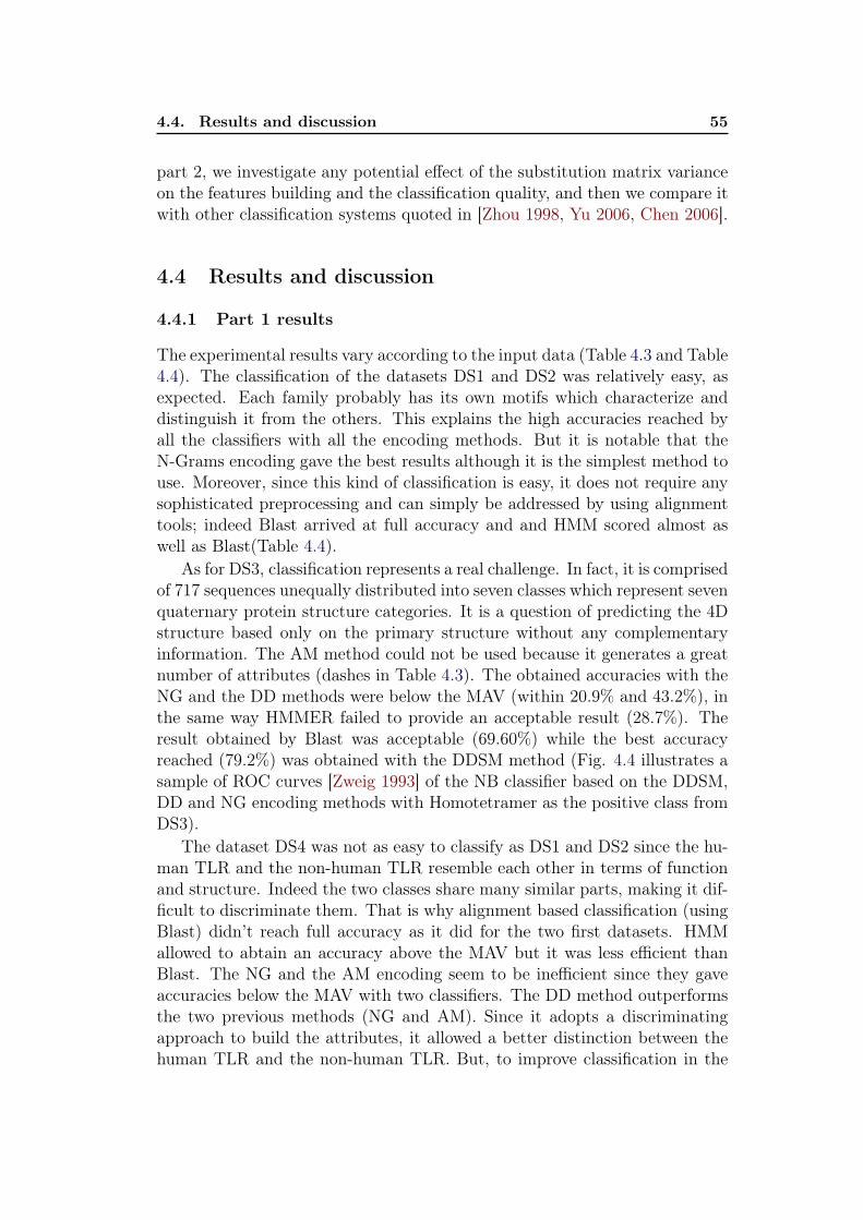
4.4. Results and discussion 55

part 2, we investigate any potential effect of the substitution matrix varianceon the features building and the classification quality, and then we compare itwith other classification systems quoted in [Zhou 1998, Yu 2006, Chen 2006].

4.4 Results and discussion

4.4.1 Part 1 results

The experimental results vary according to the input data (Table 4.3 and Table4.4). The classification of the datasets DS1 and DS2 was relatively easy, asexpected. Each family probably has its own motifs which characterize anddistinguish it from the others. This explains the high accuracies reached byall the classifiers with all the encoding methods. But it is notable that theN-Grams encoding gave the best results although it is the simplest method touse. Moreover, since this kind of classification is easy, it does not require anysophisticated preprocessing and can simply be addressed by using alignmenttools; indeed Blast arrived at full accuracy and and HMM scored almost aswell as Blast(Table 4.4).

As for DS3, classification represents a real challenge. In fact, it is comprisedof 717 sequences unequally distributed into seven classes which represent sevenquaternary protein structure categories. It is a question of predicting the 4Dstructure based only on the primary structure without any complementaryinformation. The AM method could not be used because it generates a greatnumber of attributes (dashes in Table 4.3). The obtained accuracies with theNG and the DD methods were below the MAV (within 20.9% and 43.2%), inthe same way HMMER failed to provide an acceptable result (28.7%). Theresult obtained by Blast was acceptable (69.60%) while the best accuracyreached (79.2%) was obtained with the DDSM method (Fig. 4.4 illustrates asample of ROC curves [Zweig 1993] of the NB classifier based on the DDSM,DD and NG encoding methods with Homotetramer as the positive class fromDS3).

The dataset DS4 was not as easy to classify as DS1 and DS2 since the hu-man TLR and the non-human TLR resemble each other in terms of functionand structure. Indeed the two classes share many similar parts, making it dif-ficult to discriminate them. That is why alignment based classification (usingBlast) didn’t reach full accuracy as it did for the two first datasets. HMMallowed to abtain an accuracy above the MAV but it was less efficient thanBlast. The NG and the AM encoding seem to be inefficient since they gaveaccuracies below the MAV with two classifiers. The DD method outperformsthe two previous methods (NG and AM). Since it adopts a discriminatingapproach to build the attributes, it allowed a better distinction between thehuman TLR and the non-human TLR. But, to improve classification in the



Table 4.3: Data mining classifiers coupled with encoding methods. Mtr: Metric,Clfr: Classifer, CA: Classification Accuracy(%), NA: Number of Attributes.

Encoding method

Data Mtr Clfr NG AM DD DDSM

DS1 CA C4.5 96.7 95 95 96.7SVM 96.7 93.3 96.7 96.7NB 86.7 90 81.7 80NN 63.3 78.3 60 61.7

NA 4935 2060 4905 2565

DS2 CA C4.5 99.6 99.4 99.8 99.4SVM 100 99.4 100 100NB 100 74.7 100 100NN 100 100 100 98.8

NA 6503 7055 10058 1312

DS3 CA C4.5 36.4 - 36.7 79.2SVM 43.2 - 43.2 78.94NB 43.2 - 43.1 59.4NN 20.9 - 21.3 77

NA 7983 - 8403 508

DS4 CA C4.5 60 57.5 77.5 82.5SVM 67.5 65 87.5 87.5NB 57.5 40 92.6 95NN 52.5 60 80 80

NA 5561 3602 7116 5505

DS5 CA C4.5 75.5 75.1 67.9 73.3SVM 84.1 81.2 82.3 82.3NB 77.3 63.7 84.5 85.9NN 80.5 79.4 78 78

NA 6465 2393 13830 13083

dataset DS4, it is necessary to take into account the phenomenon of muta-tion and substitution between the amino acids which constitute the proteinsequences. Indeed, the DDSM method made it possible to reach the high-est precisions with all the classifiers, while reducing the number of generatedattributes.

Experimental results obtained with DS5 show a good performance for allthe encoding methods, though no full accuracy was reached. We can notice


Table 4.4: Comparison between Blast, Hmmer and DDSM in terms of accuracy (%).

Dataset Blast Hmmer (DDSM & SVM) Best of DDSM

DS1 100 100 96.7 96.7DS2 100 99.21 100 100DS3 69.60 28.73 78.94 79.2DS4 78.57 70 87.5 95DS5 78.3 82.76 82.3 85.9

Figure 4.4: ROC curve samples for the NB classifier in the dataset DS3 with theDDSM, DD and NG encoding methods. The positive class is Homotetramer. Thisfigure shows a sample of ROC curves of the NB classifier based on the DDSM,DD and NG encoding methods with Homotetramer as the positive class (DS3). Itappears that the DDSM based ROC curve is obviously higher than the two otherones.



that NG performed very well and allowed to improve results with the classifiersC4.5, SVM and NN. Blast allowed also to obtain good accuracy which is due tothe high identity percentage within the dataset and the result was even betterwith HMMER. But, the best accuracy was obtained with DDSM (' 86%).

4.4.2 Part 2 results

In this section, we study the effect of the substitution matrice variation on theclassification by applying some of the most often used substitution matricesbelonging to the two well-known families: Blosum and Pam [Henikoff 1992,Dayhoff 1978]. These matrices are the same used by the standalone versionof Blast [Altschul 1990].

Substitution scoring is based on the substitution frequencies seen in mul-tiple sequence alignments, yet it differs from Pam to Blosum. Whereas thePam matrices have been developed from global alignments of closely relatedproteins, the Blosum matrices are based on local multiple alignments of moredistantly related sequences. This would have an effect on the representationsize. Indeed, the number of constructed features varies from a substitutionmatrix to another. Blosum matrices with low numbers and Pam matrices withhigher numbers allow the building of fewer features since they score highly thesubstitution between amino acids. This would yield larger clusters of substi-tutable motifs, and hence fewer main motifs i.e., fewer features (see Sections4.2.2 and 4.2.3). However, the variances of accuracies are slight when varyingthe substitution matrices with the same classifier (Table 4.5, Table 4.6 and Ta-ble 4.7). Moreover, no substitution matrix allows obtaining the best accuracyfor all the classifiers. We can even notice contradicting results; indeed, in DS3and DS4, NN algorithm performs worse when coupled with Pam30, while thesame matrix allows SVM to reach its best accuracy. The same phenomenon isnoticed in DS5 with the classifiers C4.5 and SVM and the matrix Pam250. Ifone looks for reduced-size representation, Blosum matrices with low numbersand Pam matrices with higher numbers are recommended.

Since we used the same dataset (DS3) and the same assessment tech-nique (leave-one-out) as in [Yu 2006], we compare our feature-building method(DDSM with default parameter values: α = 0, β = 0, substitution matrix =Blosum62, substitution probability threshold T = 0.9) with the ones studiedin [Yu 2006] (FDC, AAC, and Blast coupled each one with the nearest neigh-bor algorithm NN). Comparative results are reported in Table 4.8. We cannotice that the worst results were obtained with the AAC method. Indeed,the obtained results were below the MAV 46.7%. Blast arrived at better re-sults, but the accuracy was not very high. In fact, an analysis of the ProteinData Bank (PDB) [Berman 2000], where the protein structures are deposited,reveals that proteins with more than 30% pairwise sequence identity have sim-ilar 3D structures [Sander 1991]. But in our case we process a dataset with


Table 4.5: Experimental results per substitution matrix for DS3.

Substitution matrix Attributes Accuracy (%)

C4.5 SVM NB NN

Blosum45 377 78.5 79.2 59.4 77.7Blosum62 508 79.2 78.9 59.4 77Blosum80 532 77.6 80.5 60 77.6Pam30 2873 77.8 82 60.3 76.7Pam70 802 78.1 80.5 60.5 77Pam250 1123 77.3 79.4 59.6 78.7



C4.5 SVM NB NN

Blosum45 5095 82.5 85 95 80Blosum62 5505 82.5 87.5 95 80Blosum80 5968 72.5 87.5 92.5 80Pam30 7005 82.5 92.5 92.5 65Pam70 5846 82.5 85 92.5 80Pam250 1948 82.5 77.5 95 80



C4.5 SVM NB NN

Blosum45 12603 69.3 82.3 85.9 78Blosum62 13083 73.3 82.3 85.9 78Blosum80 13146 70.1 82.3 84.1 78Pam30 13830 69.3 82.3 84.5 78Pam70 13822 70.4 82.3 84.5 78Pam250 1969 66.1 85.2 79.4 78



Table 4.8: Comparison with results reported in [Yu 2006] for DS3.

Methods Accuracy % Correctly classified sequences

DDSM & C4.5 79.2 568DDSM & SVM 78.9 588DDSM & NB 59.4 434DDSM & NN 77 564FDC & NN 75.2 539AAC & NN 41.4 297Blast-based 69.6 499

a sequence identity of 25%. The FDC method seems to be promising since itallowed reaching an accuracy of 75.2%. But our method was quite better andenabled to reach the highest accuracy rates among the mentioned methodsand also coupled with the same classifier i.e., NN algorithm (77%). If we lookfor better classification systems we can consider the combinations (DDSM &C4.5) or (DDSM & SVM). In addition, higher accuracy can be obtained byusing the combination (DDSM & SVM) and the matrix Pam30 which enabledto reach an accuracy of 82% (Table 4.8). This indicates that SVM coupledwith our encoding method DDSM represents an efficient system for proteinclassification.

In the same way, the use of the same dataset (DS5) and the samevalidation technique (leave-one-out) as in [Chen 2006, Zhou 1998] allowedus to compare our method with these two works as well as six others[Cai 2000, Cai 2001, Cao 2006, Chou 1989, Feng 2005, Nakashima 1986]. Inthese studies, variants of the amino acid composition AAC have been proposedto encode protein sequences and then coupled with a classifier to predict theprotein structural classes. These works are based on the assumption thatthere is a strong correlation between the AAC and the structural class of aprotein. In Table 4.9, we report the results obtained by our method (DDSMwith default parameter values: α = 0, β = 0, substitution matrix = Blosum-62, substitution probability threshold T = 0.9) coupled with C4.5, SVM, NBand NN as well as the results of the related works (in Table 4.9, AACx meansthe AAC variant presented in the paper x). We can claim that our encodingmethod generally outperforms any AAC encoding method proposed by theabove-mentioned works. In [Chen 2006], authors coupled three kinds of AACwith SVM i.e., (AAC & SVM), (pair-coupled AAC & SVM) and (PseAAC &SVM). In the best case, they reached an accuracy of 80.5%, whereas the com-binations (DDSM & SVM) and (DDSM & NB) allowed reaching respectively82.3% and 85.9% of accuracy. To enhance their results, authors in [Chen 2006]proposed a fusion network that combines the results obtained by the three

4.5. Conclusion 61

proposed combinations and they arrived at an accuracy of 87.7%. Although,this result is slightly superior to ours, it does not mean that their encodingmethod outperforms DDSM. Indeed, the improvement of their results comesfrom the fusion network classifier and not from the AAC variants they use.Moreover, in most of these related works [Chen 2006, Zhou 1998, Cai 2000,Cai 2001, Cao 2006, Chou 1989, Feng 2005, Nakashima 1986], authors per-form a fine-tuning to look for the classifier parameter values allowing to getthe best results, whereas we just use the default parameter values of both ourencoding method and the classifiers as found in WEKA [Witten 2005]. Thisfine tuning allowed to reach competitive accuracies which is the case of thecombination (AAC & LogitBoost) [Feng 2005]. We believe that we can alsoreach higher accuracies if we perform a fine-tuning of the parameters of ourmethod and the classifiers. But, we chose to just use the default parametervalues to make it easier for users who may have no prior knowledge on whatthese parameters mean or how to specify them.

4.5 Conclusion

In this chapter we have proposed a new method of feature extraction to pre-process protein sequences. We have demonstrated its efficiency by comparingit with existing methods mainly in terms of classification accuracy. In the nextchapter we introduce another aspect of comparison. We explore the robust-ness of motif extraction methods with respect to perturbations within inputdata. We propose new metrics to measure that robustness.



Table

4.9:Com

parisonwith

resultsreported

in[C

hen2006]and

[Zhou1998]for

DS5.

Meth

ods

Accu

racy%

Correctly

classified

seq

DDSM

&C4.5

73.3203

DDSM

&SV

M82.3

228DDSM

&NB

85.9238

DDSM

&NN

78216

Blast-based

78.3220

AAC[Chen

2006]

&SV

M80.5

223pair-coupled

AAC[Chen

2006]

&SV

M[Chen

2006]77.6

215PseA

AC[Chen

2006]

&SV

M[C

hen2006]

80.5223

SVM

fusion[C

hen2006]

87.7243

AAC[Zhou

1998]

&Com

ponentcoupled

[Zhou1998]

79.1219

AAC[Chou

1989]

&City-block

distance[C

hou1989]

59.9166

AAC[Nakashim

a1986

]&

Euclidean

distance[N

akashima1986]

55.2153

AAC[Cai2000

]&

Neuralnetw

ork[C

ai2000]74.7

206AAC[Cai2001

]&

SVM

[Cai2001]

79.4219

AAC[Feng

2005]

&LogitB

oost[Feng

2005]84.1

233AAC[Cao

2006]

&Rough

Sets[C

ao2006]

79.4219

Chapter 5

New stability Metrics for FeatureExtraction in protein Sequences

Contents5.1 Background and related works . . . . . . . . . . . . . . . . . 645.2 Robustness of motif extraction methods . . . . . . . . . . . . 65

5.2.1 Motivations . . . . . . . . . . . . . . . . . . . . . . . . . . . . 655.2.2 Terminology . . . . . . . . . . . . . . . . . . . . . . . . . . . 675.2.3 Illustrative example . . . . . . . . . . . . . . . . . . . . . . . 68

5.3 Experiments . . . . . . . . . . . . . . . . . . . . . . . . . . . . 695.3.1 Aims and datasets . . . . . . . . . . . . . . . . . . . . . . . . 695.3.2 Protocol . . . . . . . . . . . . . . . . . . . . . . . . . . . . . . 69

5.4 Results and discussion . . . . . . . . . . . . . . . . . . . . . . 715.5 Conclusion . . . . . . . . . . . . . . . . . . . . . . . . . . . . . 75

GoalsSeveral previous works have described feature extraction methods for bio-sequence classification, but none of them discussed the robustness of thesemethods when perturbing the input data. In this chapter, we introduce thenotion of stability of the generated motifs in order to study the robustness ofmotif extraction methods. We express this robustness in terms of the abilityof the method to reveal any change occurring in the input data and alsoits ability to target the interesting motifs. We use these criteria to evaluateand experimentally compare four existing extraction methods for biologicalsequences. The subject of this chapter has been published in [Saidi 2010a,Saidi 2012a].

64Chapter 5. New stability Metrics for Feature Extraction in protein

Sequences


Several motif extraction methods have been proposed. Meanwhile, variousstudies have made assessments and comparisons between these methods andhave tried to study the impact of one method or another on the quality of thelearning task to be performed (classification, prediction, shape recognition,etc). So, the best methods are those that allow having the best values ofquality metrics such as accuracy rate in the case of supervised classification.

In this chapter, we introduce the concept of stability to compare motifextraction methods. We call stability of a motif extraction method from adataset, the non-variability in its set of motifs, when applying a technique ofvariation on the input data. The robustness of a method is the coupling ofthe non-stability and the ability to retain or improve the quality of the asso-ciated data mining task. In our case, we will use the supervised classificationaccuracy as a quality measure.

Concrete motivations behind the above-mentioned stability can be foundwithin distributed systems and grid computing environments that are mininghuge amounts of data. In such environments, the variation of data is a commonfact. This variation can be due to various events such as failed transfer of dataportions, loss of communication between nodes of the distributed system, dataupdating, etc. Another motivating application is information retrieval frombiological databases (such as GenBank [Benson 2009], EMBL[Stoesser 2002],UniProt[Bairoch 2005]). The problem here lies in the fact that every databasehas its own terminology and procedures which sometimes yield related but notidentical data [Zhao 2008]. Since the retrieved data are the main materials ofseveral delicate processes in both industry and research like disease manage-ment and drug development, it is crucial for database researcher, bioscienceuser and bioinformatics practitioner to be aware of any change in the prepara-tion data samples [Topaloglou 2004]. In addition, with the exploding amountsof data submitted to the biological databases, there is an increasing possibilityof finding erroneous data. In such conditions, it is important to make surethat the motif extraction methods, which are the start point of any miningprocess, are robust enough to detect even slight variations in input data likedoes any good sensor when describing its context environment.

The topic of stability with respect to motif extraction methods has notbeen studied in the literature. However, this aspect was slightly studied ina very close field to the extraction which is the feature selection [Pavel 2007,Yvan 2008, Dunne 2002, Kalousis 2007, Somol 2008, Yu 2008].

In [Pavel 2007], authors propose a measure which assesses the stability offeature selection algorithms with respect to random perturbation in data. Inthis work, the stability of feature selection algorithms can be assessed throughthe properties of the generated probability distributions of the selected feature

5.2. Robustness of motif extraction methods 65

subsets. The interestingness is, of course, in feature selection algorithms thatproduce probability distributions far from the uniform and close to the peakone. Given a set of features, all possible feature combinations of size k areconsidered achieving n feature subsets. The frequencies F of selected featuresubsets are recorded during data perturbation in a histogram. For a size k,the stability Sk is measured based on the Shannon entropy:

Sk = −n∑i=1

Fi logFi . (5.1)

In [Yvan 2008], authors perform an instance sub-sampling to simulate dataperturbation. Feature selection is performed on each of the n sub-samples,and a measure of stability is calculated. The output f of the feature se-lection applied on each sub-sample is compared to the outputs of the othersub-samples using Pearson correlation coefficient [Cohen 1988], the Spearmanrank correlation coefficient [Yule 1950] and the Jaccard index [Real 1996] assimilarity measure noted S. The more similar all outputs are, the higher thestability measure will be. The overall stability can then be defined as theaverage over all pairwise similarity comparisons:

Stotal =2×

∑n−1i=1

∑nj=i+1 S(fi, fj)

n(n− 1). (5.2)

In [Dunne 2002], different sub-samples (or training sets) are created usingthe same generating distribution. Stability quantifies how different trainingsets affect the feature selection output. Authors take into account three typesof representations for feature subsets. In the first type, a weight or score isassigned to each feature indicating its importance. The second type of repre-sentation, ranks are assigned to features. The third type consists only of setsof features in which no weighting or ranking is considered. Measuring stabil-ity requires a similarity measure for feature representations. This obviouslydepends on the representation used by a given feature selection algorithm todescribe its feature subset. The authors used three similarity measures: thePearson’s correlation coefficient, the Spearman rank correlation coefficient andthe Tanimoto distance.

5.2 Robustness of motif extraction methods

5.2.1 Motivations

The application of the above-presented measures of stability is not conve-nient in our case (motif extraction). This originates from the nature of in-put data used by feature selection methods [Ma 2008, Saeys 2007, Liu 2007,Sebban 2002]. In fact, these methods use an original set of features (motifs)


Sequences

Figure 5.1: Data perturbation in feature selection and motif extraction

as input and try to merely select a subset of relevant features. The pertur-bation of data is applied to the original set of features. In the case of motifextraction, the input data are still in raw state and the data perturbation stepis applied directly to raw data (before motif extraction step)(Fig. 5.1).

In our work, the motivation behind exploring the motif extraction methodstability is to provide evidence that even slight changes in the data must alsobe followed by changes in the output results (extracted motifs). These changesmust concern the motifs that are no longer significant for the perturbed inputdata; which means that the motifs that have been conserved must prove tobe interesting i.e., help with better classification. Since the set of featuresare not known a priori we can not apply the measures quoted in the featureselection related works. For our purposes let be the two following assumptions:

Assumption 1. We consider that a motif extraction method allows areliable description of input data if any variation within these data affects theset of the generated motifs. That is to say that it reveals any change occurringin the input data.

Assumption 2. After changes in the set of generated motifs, the motifsthat are conserved should be interesting i.e., help with better classification.

In the next subsection we define and describe the terms we use to formallyexpress our assumptions and to evaluate the robustness of motif extractionmethods.

5.2. Robustness of motif extraction methods 67

5.2.2 Terminology

Based on Assumption 1, we introduce the concept of sensibility . This con-cept reflects the ability to produce a different set of motifs i.e., a differentdata description, whenever we make a variation within the input data. Thesensitivity criterion can be studied by means of the conserved motifs calledstable motifs. It is also interesting to test the Assumption 2, that is to say thequality of the stable motifs, by assessing their benefits in an artificial learningtask.

Below we formally define the terms used in this paper. Consider the fol-lowing:

- A dataset D, divided into n subsets D1, D2,.., Dn.

- A motif extraction methodM applied to D on one side and to D1, D2,..,Dn on the other side and respectively generating the sets of motifs SMfrom D and SM1, SM2, .., SMn from D1, D2,.., Dn.

- An artificial learning task T and a quality metric Mtr of T . LetMtrT (SM) denote the value of the metric obtained if T is performedusing the set SM as a feature space.

We define the following:

Definition 21 (Motif Stability) A motif x is said to be stable if and onlyif its occurrence rate in all SMi, i = 1..n, exceeds a threshold . The occurrencerate is simply the ratio of the number of SMi, i = 1..n, where x appears to n.Formally:

Number of SMi/x ∈ SMi

n≥ τ, with i = 1..n . (5.3)

Definition 22 (Rate of stable motifs) The rate of stable motifs (RSM)of a method M is the ratio of the number of stable motifs to the number ofdistinct motifs of all SMi, i = 1..n. Formally:

RSM =Number of stable motifs

|⋃ni=1 SMi|

. (5.4)

Definition 23 (Method sensibility) A method M1 is more sensible thananother methodM2 if and only if for the same changes within the same dataset,the rate of stable motifs of M1 is lower than that of M2. Thus, the sensibilityS of a method is complementary to its rate of stable motifs. It may be noted:

S = 1−RSM . (5.5)

Definition 24 (Conservation of the quality metric value) A motif ex-traction method M conserves the quality metric value of a data mining task


Sequences

T if the use of the set of stable motifs SSM in T preserves the quality metricvalues for this task as when we use the set of motifs SM generated from theoriginal dataset D. However, it is noteworthy that we can not judge that con-servation unless the method is already sensible. Indeed, an insensible methodtends to generate the same motifs even after perturbations in the input dataindicating that its extraction approach is rigid and does not adopt a conceptof "choice". This conservation C can be measured by:

C = 1− |MtrT (SM)−MtrT (SSM)| . (5.6)

Definition 25 (Interestingness of a set of stable motifs) A set of sta-ble motifs SSM is considered to be interesting if it allows interesting values ofconservation and sensibility. Formally, we can measure this interestingness Iby:

I = 2× S × CS + C

. (5.7)

This measure is inspired from the F1-Score which is a statistical measureof a test’s accuracy that combines Precision and Recall. The F1-score can beinterpreted as a weighted average of the precision and recall, where an F1-score reaches its best value at 1 and worst score at 0. In our case, we combineconservation and sensibility to quantify the interestingness of stable motifs.


Considering a dataset D in a supervised classification task T . The data per-turbation of D generates three subsets D1, D2 and D3. The application of amotif extraction methodM to D on one side and to D1, D2 and D3 on anotherside generates the sets of motifs SM from D and SM1, SM2 and SM3 fromD1, D2 and D3 respectively :SM =m1, m2, m3, m4, m5, m6, m7, m8, m9, m10SM1=m1, m4, m5, m6SM2=m1, m2, m3SM3=m1, m6, m7, m8

Using τ such that τ = 65%, the motifs m1 and m6 are considered stablesince they appear in more than 65% of the motifs subsets.We can easily calculate the rate of stable motifs RSM = 0.25, which is twoover the set of eight motifs. We consider that m9 and m10 are noise, and thusare not relevant for the classification task.The sensibility of M is calculated by S = 0.75.

In this case, the set of stable motifs SSM1 = m1, m6.Using τ > 66%, only the motif m1 are considered stable since it appears

in more than τ% of the motifs subsets.We can easily calculate the rate of stable motifs RSM = 0.125.The sensibility of M is calculated by S = 0.875, and SSM2 = m1.

5.3. Experiments 69

Suppose we use sets of motifs SM and SSM1 as variables space to measurethe accuracy rate (MtrT ) of the supervised classification task T . Let considerthe following obtained values with MtrT :Mtr(SM) = 0.85Mtr(SSM) = 0.80

The set of stable motifs SSM1 enables a conservation of the quality metricvalue C = 0.95 Finally, we can measure the interestingness of stable motifsby I = 0.83.

5.3 Experiments

In this section, we describe an experimental study conducted on four motifselection methods quoted in [Saidi 2010b]. Calculations were run on a duoCPU 1.46GHz PC with 2GB memory, operating on Linux. The following is apresentation of the input datasets and the used tools.

5.3.1 Aims and datasets

We used four datasets containing 1327 protein sequences extracted from Swiss-Prot [Bairoch 2000] and described in Table 5.1. These datasets differ from oneanother in terms of size, number of class, class distribution, complexity andsequence identity percentage. The change in the nature of the datasets allowsus to avoid specific outcomes to data and to have better interpretations. Moredescription of data can be found in Chapter 4.

We compare the motif extraction methods quoted in chapter 4[Saidi 2010b], i.e., n-grams NG [Leslie 2002], active motifs AM [Wang 1994],discriminative descriptors DD [Maddouri 2004] and discriminative descriptorswith substitution matrix DDSM [Saidi 2010b]. In our experiments, we use thesame default settings as in [Saidi 2010b].

Comparisons made in [Saidi 2010b] between these methods revealedthat DDSM performs the best to help in problems of protein sequencesclassification even in difficult cases where other methods fail to producereliable descriptors for an accurate classification. In this work, we try tofind a relationship between this performance and the concepts introduced inSection 5.2.2.

5.3.2 Protocol

In our experiments, we perturb each input dataset in a systematic way andwe observe the impact of this perturbation on the set of generated motifs. Todo this, several perturbation techniques can be adopted :


Sequences

Table 5.1: Experimental data.

Dataset Family / class

DS1High-potential Iron- Sulfur ProteinHydrogenase Nickel Incorporation Protein HypAGlycine Dehydrogenase

DS2Human TLRNon-human TLR

DS3ChemokineMelanocortin

DS4

MonomerHomodimerHomotrimerHomotetramerHomopentamerHomohexamerHomooctamer

1. Removing and/or adding of sequences: This technique can be simulatedby eliminating some sequences from the dateset.

2. Perturbing the sequences: This can be done by modifying amino acidswithin sequences.

In our experiments, we perturb each input dataset in a systematic wayand we observe the impact of this perturbation on the set of generated motifs.To do this, we use the 10-cross-validation (10CV) and leave-one-out tech-niques (LOO) [Han 2006]. Therefore, the variation of a dataset containing nsequences consists in removing a partition (one tenth with 10-cross-validationand a single sequence with leave-one-out) from the dataset and the rest is usedto generate a set of motifs. This is done several times (ten times with 10-cross-validation and n times with leave-one-out). At each iteration, the number ofoccurrences of generated motifs is updated. As already defined in Section5.2.2, the technique we adopt to measure the sensibility of motif extractionmethods from protein sequences is based on the rate of stable motifs. Whereasthe sensibility is related to the amount of stable motifs, the interestingnessof stable motifs is related to their quality. In other words, if these motifsare generated by the extraction method to appear often enough then theyshould be "interesting". We measure the interestingness in our experimentsby their usefulness in a supervised classification task. Once the stable motifsare generated, they are used to convert protein sequences into binary vectorswhere the value ’1’ denotes the presence of motif in the sequence and ’0’ its


Figure 5.2: Experimental process

absence, all these binary vectors compose what is called a learning context.Thus the classification of proteins in this new format is now possible with datamining tools. To do this, we use the support vector machine classifier SVMof WEKA workbench [Witten 2005]. The classification is performed basedon 10-cross-validation (10CV) and leave-one-out (LOO) techniques. Hence,our experiments are conducted using the following four combinations for datavariation and classification: (LOO; LOO), (LOO; 10CV), (10CV; LOO) and(10CV; 10CV).


We show in Table 5.2 the classification results of our datasets using the fourmotif extraction methods. The classification is performed without making anyperturbation on our datasets using the SVM classifier of WEKA [Witten 2005]based on 10-cross-validation (10CV) and leave-one-out (LOO). Comparingthese results with those obtained using the stable motifs allows us to betterevaluate the studied methods and test Assumption 1 and 2.

The experimental results are presented in Table 5.3 and 5.4. Table 5.3contains the results obtained with a LOO based variation and Table 5.4 with10CV based variation. For each dataset and for each value of τ , we note therate of stable motifs and their corresponding accuracy if we use these motifsto classify protein sequences of that dataset based on 10-cross-validation andleave-one-out tests. We can notice that the classification test technique i.e.,10CV or LOO does not affect the obtained results (the interestingness ratesare almost the same). Using results from Table 5.2, 5.3 and 5.4, we draw theinterestingness of stable motifs histogram corresponding to dataset (Fig. 5.3


Sequences

Table 5.2: Accuracy rate of the studied methods using datasets without modifica-tion.

MethodDS1 DS2 DS3 DS4

10CV LOO 10CV LOO 10CV LOO 10CV LOO

NG 96.7 96.7 67.5 67.5 100 100 44.9 45.5AM 100 100 72.5 65 100 100 - -DD 96.7 96.7 82.5 80 100 100 43.5 43.5DDSM 96.7 96.7 95 95 100 100 82.5 87.5

and 5.4).We notice that NG is virtually insensible to variations in data. Indeed,

its rate of stable motifs is often equal or very close to 100%. Therefore, thevariation of input data has no bearing on the generated motifs. In other words,we often obtain the same motifs even in the presence of variations in inputdata. In this case, we can not evoke the interestingness of stable motifs (seeFig. 5.3 and 5.4).

The AM method follows almost the same fluctuating behavior for alldatasets (except for DS4 where we could not conduct our experiments dueto lack of memory). In fact, below τ = 0.7, AM is insensible (RSM is equalor close to 100%). Beyond this value, AM becomes sensible. This sensibilityvaries depending on dataset and the variation technique (10CV or LOO). Itis very significant for DS1, average for DS2 and slight for DS3. For examplein Table 5.3, for τ = 0.7, the rate of stable motifs are 32.5, 83.6 and 98.3%,respectively for DS1, DS2 and DS3. Similarly, the interestingness of stableAM motifs is very fluctuating and varies as well depending on the dataset (seeFig. 5.3 and 5.4). This method is sometimes completive to DD and DDSM.But, we note that it is greedy in memory and can not handle large datasetsas it is the case with the dataset DS4 (see Table 5.3 and 5.4).

The approach adopted by the DD method offers it a sensible nature. Infact, according to this method, each motif must satisfy the conditions of dis-crimination and minimality (see Chapter 4). Therefore, it is likely that a dis-ruption of input yields not meeting these conditions and thus the eliminationof some existing motifs and/or addition of new ones. At the same time, thismethod generates sets of interesting stable motifs with all the data samplesand different values of τ . Indeed, it generally allows better interestingnessrates than NG and AM (see Fig. 5.3 and 5.4).

The DDSM method is an extension of DD, which adopts a competitiveapproach among the motifs to generate. Indeed, to be chosen, a motif must bethe most mutable among other ones of equal size. This constraint remarkablyincreases the sensibility of the method vis-a-vis the changes in the input data.

5.4. Results and discussion 73Tab

le5.3:

Rateof

stab

lemotifs

andtheirclassific

ationaccu

racy

usingLO

O-based

variation.

DS

τ

Rateof

stab

lemotifs

Classification

accu

racy

rate

NG

AM

DD

DDSM

NG

AM

DD

DDSM

10CV

LOO

10CV

LOO

10CV

LOO

10CV

LOO

DS1

0.5

100

100

8163

96.7

96.7

100

100

96.7

96.7

100

100

0.6

100

100

8160

.596

.796

.710

010

096

.796

.710

010

00.7

100

32.5

8159.7

96.7

96.7

100

100

96.7

96.7

100

100

0.8

100

31.6

80.8

59.1

96.7

96.7

100

100

96.7

96.7

100

100

0.9

100

31.6

80.7

58.6

96.7

96.7

100

100

96.7

96.7

100

100

169

.31.8

0.01

0.02

96.7

96.7

93.3

93.3

6028

.330

0

DS2

0.5

100

100

7962

.867

.567

.572

.565

82.5

8095

950.6

100

100

7962

.467

.567

.572

.565

82.5

8095

950.7

100

83.6

76.9

58.4

67.5

67.5

6562

.580

77.5

92.5

92.5

0.8

100

83.6

76.8

57.7

67.5

67.5

6562

.580

77.5

9092

.50.9

100

83.6

76.7

55.5

67.5

67.5

6562

.580

77.5

92.5

92.5

174

.60.4

0.05

0.01

6567

.562.5

62.5

6565

6565

DS3

0.5

100

100

95.6

86.7

100

100

100

100

100

100

99.8

99.8

0.6

100

100

95.5

85.5

100

100

100

100

100

100

99.8

99.8

0.7

100

98.3

95.2

83.9

100

100

100

100

100

100

99.8

99.8

0.8

100

98.3

95.1

83.1

100

100

100

100

100

100

99.8

99.8

0.9

100

98.3

94.7

8110

010

010

010

010

010

099

.899

.81

87.9

1.23

0.01

0.1

100

100

9797

.195.3

95.3

490

DS4

0.5

100

-98

.884

.144

.945

.5-

-45

4670

.269

.20.6

100

-98

.884

.144

.945

.5-

-45

4670

.269

.20.7

100

-98

.884

.144

.945

.5-

-45

4670

.269

.20.8

100

-98

.883

.644

.945

.5-

-45

4669

.969

.50.9

100

-98

.773

.244

.945

.5-

-45

4669

.870

.91

90-

0.01

6944

.945

.5-

-46

.746

.770

.670


SequencesTable

5.4:Rate

ofstable

motifs

andtheir

classificationaccuracy

using10C

V-based

variation.

DS

τ

Rate

ofstab

lemotifs

Classifi

cationaccu

racyrate

NG

AM

DD

DDSM

NG

AM

DD

DDSM

10CV

LOO

10CV

LOO

10CV

LOO

10CV

LOO

DS1

0.5100

98,479,9

62,196.7

96.798.3

98.396.7

96.7100

1000.6

10096

79.759.9

96.796.7

98.398.3

96.796.7

100100

0.7100

38,574,5

49,296.7

96.798.3

98.396.7

96.7100

1000.8

10028.1

66.137.3

96.796.7

100100

96.796.7

100100

0.964,6

14,830,8

14,596.7

96.7100

10096.7

96.7100

1001

64.614.8

30.814.5

96.796.7

100100

96.796.7

100100

DS2

0.5100

94,364,6

49,165

67.562.5

6592.5

92.562.5

62.50.6

10080

6446.6

6567.5

6065

92.592.5

6567.5

0.7100

60,654,4

31,265

67.565

67.595

9565

650.8

10046.5

38.216.7

6567.5

67.570

92.595

57.565

0.9100

32,19,5

4,165

67.567.5

7092.5

92.537.5

351

70.132.1

9.54.1

6567.5

67.570

92.592.5

37.535

DS3

0.5100

97,180,3

62,8100

100100

100100

10099.8

99.80.6

10069.3

8060.9

100100

100100

100100

99.899.8

0.7100

52,475,8

51,8100

100100

100100

10099.8

99.80.8

10048.5

63.838

100100

100100

100100

99.899.8

0.984,3

40,533

17,1100

100100

100100

10099.8

99.81

84.340.5

3317.1

100100

100100

100100

99.899.8

DS4

0.5100

-100

86.244.89

45.47-

-45.19

45.8970.2

69.20.6

100-

10086.2

44.945.5

--

45.245.9

70.269.2

0.7100

-100

83.544.9

45.5-

-45.2

45.970.4

69.30.8

100-

10078.8

44.945.5

--

45.245.9

69.570

0.999,4

-99,4

72.844.9

45.5-

-45.2

45.970.6

711

99.4-

99.472.8

44.945.5

--

45.245.9

70.671

5.5. Conclusion 75

This can be noticed by the decreasing rates of stable motifs compared to theDD method. In addition, this high sensibility is always accompanied by a setof very interesting stable motifs manifested by generally allowing the highestinterestingness rates. However, we note that for τ = 1, DDSM does not oftenhave the best rates of interestingness especially with 10CV based variation(we recall that this value of τ means that the stable motifs are those thatappear in all variations of data). This is because the substitution, which is afundamental criterion in the process of DDSM, is not taken into account in theconstruction of the set of stable motifs. Hence, similar forms of a given motifmay be ignored. But by relaxing the condition of τ = 1 and moving to smallervalues of τ we see that the interestingness rates get improved considerably.This method reveals both the property of sensibility and interestingness of itsstable motifs (see Fig. 5.3 and 5.4), which allows it to redescribe well the inputdata, which is in accordance with results of Chapter 4 showing the efficiencyof this method for feature extraction in protein sequences.

5.5 Conclusion

In this chapter, we introduced the notions of stability and sensibility as newcriteria to compare motif extraction methods from biological sequences. Thesensibility of a method is its ability to produce a different set of motifs, so adifferent description, whenever a perturbation is made in the dataset. Thiscriterion must be accompanied by a set of interesting stable motifs. Thisconcept of interestingness arises when a method eliminates certain motif andconserves others following a change in the input data and that the conservedmotifs are useful if used in a data mining task. The experimental study showsthat the DDSM method is more sensible compared to the other methods. Thissensibility is usually accompanied by sets of stable interesting motifs. Thisconfirms the results of Chapter 4 that show the contribution of the DDSMmethod in supervised classification tasks. In the next chapter, we explorethe second axis of this thesis by studying the different approaches of graph-representation of proteins.


Sequences

Figure

5.3:Interestingness

ofstable

motifs

usingLO

O-based

variation

5.5. Conclusion 77

Figure5.4:

Interestingn

essof

stab

lemotifs

using10

CV-based

variation

Chapter 6

Graph-based representations ofprotein structures

Contents6.1 Background . . . . . . . . . . . . . . . . . . . . . . . . . . . . . 806.2 Proteins and graphs . . . . . . . . . . . . . . . . . . . . . . . . 81

6.2.1 Amino Acids and vertices . . . . . . . . . . . . . . . . . . . . 816.2.2 Chemical Interactions that stabilize Proteins . . . . . . . . . 82

6.3 Building graphs from protein structures . . . . . . . . . . . . 846.3.1 Main atom . . . . . . . . . . . . . . . . . . . . . . . . . . . . 846.3.2 All atoms . . . . . . . . . . . . . . . . . . . . . . . . . . . . . 866.3.3 Triangulation . . . . . . . . . . . . . . . . . . . . . . . . . . . 87

6.4 Experimental comparison . . . . . . . . . . . . . . . . . . . . 896.5 Conclusion . . . . . . . . . . . . . . . . . . . . . . . . . . . . . 91

GoalsIn this chapter, we make a brief survey on various existing graph-based repre-sentations and propose some tips to help with the protein graph making sincea key step of a valuable protein structure learning process is to build conciseand correct graphs holding reliable information. We, also, show that someexisting and widespread methods present remarkable weaknesses and do notreally reflect the real protein conformation. The subject of this chapter hasbeen published in [Saidi 2009].

80 Chapter 6. Graph-based representations of protein structures

6.1 Background

The structural database PDB [Berman 2000] continues to expand tremen-dously comprising so far more than 77000 protein structures. Hence, newmethods are required to analyze, study and compare protein structures.Whereas the recognition, comparison, and classification of sequences is nowmore or less a solved problem, accurate computational and data mining toolsfor the study of the proteins in their native state are still not abundant[Kleywegt 1999, Doppelt 2007].

The investigation of 3D protein structures can give important functionaland structural insights whereas the sequences fail to provide full accurateinformation especially in function prediction tasks [Doppelt 2007]. Indeed,during the evolution some distantly related proteins may lose sequence homol-ogy while retaining some common folding. A primordial step to any miningprocess or any computational study of proteins is to look for a convenientrepresentation of their spatial conformation i.e., a preprocessing step is nec-essary to yield computer-analyzable data [Saidi 2010b]. Since proteins aremacromolecules that can be viewed as a set of related elements (amino-acids,atoms, etc), they can be translated into graphs where vertices may vary fromatoms to coarser sub-structures like secondary structure fragments. In mostworks that studied proteins as graph structures, vertices have been repre-sented by amino acids, the basic building blocks of proteins. In fact, aminoacids are better to express any conformation homology between protein struc-tures than using atoms or secondary structure elements. Besides, that maygive valuable extensions to the previous works on sequences like motif discov-ery [Kleywegt 1999][Doppelt 2007].

We review several existing methods and show that they comprise funda-mental points of criticisms. Based on these criticisms, we try to enhance theprotein graph making. It is very important to build a graph-based represen-tation that reflects the real protein conformation since it will be the startingpoint of any later processing and analysis.

In the next section, we try to make the matching between proteins andgraphs in a structural view while explaining what makes proteins performtheir 3D shape and introducing any technical term we use in the protein graphbuilding. Section 6.3 exhibits the most used preprocessing methods of graphmaking from proteins as well as our suggestions to enhance this task. In Sec-tion 6.4, we experimentally compare two methods. Some recommendations,concluding points can be found in Section 6.5.

6.2. Proteins and graphs 81

6.2 Proteins and graphs

A graph is a finite set of vertices (or nodes) and edges (or arcs) defined ascouples G = (V,E) where V is the set of vertices and E is the set of edges.Each element of E i.e., edge is a pair of adjacent vertices of V . Graphs haveextensively been used to investigate various real applications such as commu-nication and transportation networks, electrical circuits, chemical componentsand recently to investigate the protein structure analysis [Vishveshwara 2002].

Proteins are biological macromolecules formed by concatenation of 20 dis-tinct amino acids into long chains. They play crucial roles in almost everybiological process. They are responsible in one form or another for a variety ofphysiological functions including enzymatic catalysis, binding, transport andstorage, immune protection and control of growth, etc.

The sequence of the amino acid residues in these chains is termed the pro-tein primary structure. These chains can fold to form complex 3D structuresdue to a combination of chemical interactions with the existence of some stan-dard sub-structures called secondary structures. In the final folded state of aprotein i.e., tertiary structure, residues that are far away in the chain can bevery close in space.

From a computer science point of view, the protein structure can be viewedas a set of elements. Each element can be an atom, an amino acid residue or asecondary structure fragment. Hence, several graph representations have beendeveloped to preprocess protein structure, ranging from coarse representationsin which each vertex is a secondary structure fragment to fine representationsin which each vertex is an atom [Vishveshwara 2002].

In this chapter, we consider the graph representations that use amino acidsas vertices, since amino acids are the basic structural building units of anyprotein which give it its properties and specify its spatial conformation. Be-sides, any spatial motif is more valuable if expressed in term of amino acidsthan atoms or secondary structure elements. This kind of spatial motifs givemore information about distant proteins sharing similar functions.

6.2.1 Amino Acids and vertices

The amino acids, which are supposed to be the vertices of the graph, repre-sent the basic building units of proteins. We recall that there exist 20 aminoacids sharing a common structural scheme. An amino acid is composed ofa central (but not the centroid) carbon atom called Cα and four chemicalgroups attached to Cα: a hydrogen atom, an amino group, a carboxyl groupand a side chain or radical R (Fig. 6.1). It is the side chain that differenti-ates one amino acid to another and gives it its physico-chemical properties.The common parts between the amino acids compose the so called backbone[Brandon 1991].


Figure 6.1: Amino acid structure and protein primary structure.

As we have mentioned, amino acids are linearly linked together to formthe protein sequence called primary structure [Brandon 1991]. But the pro-tein does not keep that linearity and continue to fold into a 3D compact shapewhile having local standard fragments called secondary structure due to hy-drogen bonds between backbone atoms (see Chapter 2). The determinationof the folded structure of a protein is a lengthy process, involving complicatedmethods like X-ray crystallography. X-ray method is the most accurate andmost used method; it covers 86.5% of the released protein structures but itdoes not make hydrogen atoms visible.

6.2.2 Chemical Interactions that stabilize Proteins

Chemical interactions are the forces that hold atoms and residues together,forming molecules. The chemical interactions that stabilize proteins and givethem their 3D shape can be divided into five groups: covalent bonds in whichatoms share electrons, ionic bonds, hydrogen bonds, hydrophobic interactions,and Van der Waals forces [Brandon 1991].

When talking about protein graph building, these interactions are sup-posed to be, in one form or another, the chemical analogues of the graphedges.

6.2.2.1 Covalent Bonds

Covalent bonds involve the sharing of a pair of valence electrons by two atomsand they are the strongest chemical bonds contributing to the protein struc-ture. In fact, protein chains are held together by covalent bonds linking be-tween neighboring amino acids that compose the primary structure, they arealso called peptide bonds and formed when the carboxyl group of one aminoacid reacts with the amino group of the other amino acid, thereby releasing

6.2. Proteins and graphs 83

a molecule of water (H2O). Peptide bonds have a typical distance of 1.5 . Aswell, covalent bonds between cysteine side chains can be important determi-nants of protein structure like in human insulin (2HUI in the PBD). Cysteineis the one and only amino acid whose side chain can form covalent bondswith other cysteine side chains. This type of covalent bond is called disulfidebridges and its length vary from to 1.8 to 3 [Steudel 1975].

6.2.2.2 Ionic Bonds

Ionic bonds, also called salt bridges, are distance-depending electrostatic at-tractions between oppositely charged components [Brandon 1991]. The closerthe charged components are, the stronger the attraction is. Ionic bonds arerare, however, they can be important to protein structure since they allow po-tent electrostatic attractions approaching the covalent bond strength. Typicalionic bonds bridges have lengths of around 3.0 .

6.2.2.3 Hydrogen bonds

Hydrogen bonds (or shortly H-bonds) arise when two partially negativelycharged atoms share a partially positively charged hydrogen [Brandon 1991].Many combinations of H-bond are possible:

- Atoms on two different amino acid side-chains.

- Atoms on amino acid side-chains and protein backbone atoms.

- Backbone atoms on two different amino acids (like in secondary struc-tures).

The range of this bond, which is the distance between the two atoms thatshare the hydrogen atom, is typically around 3.5 .

6.2.2.4 Hydrophobic interactions

Hydrophobic interactions are the most important non-covalent forces thatmake the compact shape of the protein structure. They arise when hydropho-bic amino acids in the protein closely associate their side chains together inan aqueous solvent, forming interior hydrophobic protein core shielded frominteractions with water [Brandon 1991].

6.2.2.5 Van der Waals forces

The Van der Waals forces are a transient, weak electrical attraction of oneatom for another when electrons are fluctuating. Electrons fluctuation yieldsa temporary electric charge which induces a complementary dipole in another


atom. Van der Waals forces are short range bonds with a radius of about 2[Bondi 1964].

6.3 Building graphs from protein structures

In the representations that use amino acids as vertices, edges are usuallydefined based on distance between these vertices. However, some works ex-pressed that edge by the strength of interaction between two amino acid sidechains [Brinda 2005]. Hereafter, we mention the most widespread methods ofprotein graph building and try to give some tips to help with the enhancementof such task. Proteins are described by PDB files [Berman 2000] including theatoms coordinates among other information.

We assume that the correctness of a protein graph is directly linked to howmuch the existing edges reflect the really existing interactions that stabilize theprotein even the interactions responsible of maintaining secondary structures.

Initially, we connect the vertices corresponding to the consecutive aminoacids in the primary structure.

6.3.1 Main atom

Generally, works that use graphs as a means to represent proteins, abstracteach amino acid u to a sole main atom of u denoted by MAu and charac-terized by its spatial coordinates (xu, yu, zu). This main atom can be reallike Cα or C1

β atoms or virtual like the amino acid centroid or the side chaincentroid [Lovell 2003, Huan 2005]. Two vertices u and v are said linked byan edge e(u, v) = 1 if the euclidian distance between their two main atoms∆(MAu,MAv) is below a threshold distance δ . Formally:

e(u, v) =

1 if∆(MAu,MAv) ≤ δ0 otherwise

(6.1)

∆(MAu,MAv) =√

(xu − xv)2 + (yu − yv)2 + (zu − zv)2 (6.2)

The time complexity of such methods is O(n2) where n is the number of aminoacids.

By reviewing the literature, we found that many works use Cα atoms asmain atoms and sometimes Cβ with usually δ ≥ 7 on the argument that Cαatoms define the overall protein conformation [Huan 2005]. We experimentallytried to assess these ways of graph building and to check whether they can findalready known links/bonds in proteins by making the graphs of some PDBfiles namely, the human insulin (2HIU). We noticed that to discover some trueedges (disulfide bridges, secondary structures, etc) using Cα, δ must not bebelow 7 . However, such threshold would yield many false edges depending

6.3. Building graphs from protein structures 85

Figure 6.2: Distance between the centroids is not enough. Size of side chains mustbe taken into account: for the same ∆, we notice that in the upper figure, the factthat ∆ ≥ δ matches with the existence of a chemical bond since the side chainboundaries are enough close to each other which is not the case for the lower figure.

on the positions and orientations of amino acids. Indeed, it is obvious thatwe can find many amino acids, whose Cα atoms are within the range of 7and even less, which are not concerned by any chemical interaction especiallywhen their side chains are far away to each other. Using high threshold greatlyincreases the number of edges without really matching with existing chemicalinteractions i.e., false edges. Whereas using low threshold does not help withfinding true edge especially in the case of amino acids having big side chainsmaking Cα atoms far away from each other. The same criticisms can beinduced concerning the use of Cβ.

As for the use of the side chain centroid (or radical centroid RC), thismethod is better to detect bonds between side chains. But, it is weak con-cerning bonds linking backbones to backbones or backbones to side chains.It presents another weakness since it does not take into account the size ofside chains which differs from an amino acid to another, so a threshold δ thatallows to reflect a real chemical interaction between two side chains does notnecessarily do the same for two other side chains especially when they aresmall in size (see Fig. 6.2). We recommend assimilating the side chain into asphere with a ray ρ, to use lower threshold and to replace Formula 6.1 by the


following:

e(u, v) =

1 if∆(RCu, RCv)− (ρu + ρv) ≤ δ0 otherwise

(6.3)

The use of the amino acid centroid may be better than using Cα or Cβ. Butthis method is also concerned by the remarks on the importance of taking intoaccount the size of the amino acids. So, similar formula to Formula 6.3 canbe utilized.

6.3.2 All atoms

Since atoms are directly concerned by bonding, one can think of build-ing edges by examining distances between all atoms of two given aminoacids. We did not find in the literature any work that uses this methodto build graphs of amino acids, but it has been used with graphs of atoms[Jacobs 2001, Keating 2009]. The principle is similar to the one in Section6.3.1: Two vertices u and v are said linked by an edge e(u, v) = 1 if thereexist two atoms Au, Av belonging respectively to u and v and whose euclidiandistance ∆(Au, Av) is below a threshold distance. Formally:

e(u, v) =

1 if ∃ Au ∈ u and Av ∈ v : ∆(Au, Av) ≤ δ0 otherwise

(6.4)

The time complexity of such methods is O(n2 ∗m2) where n is the numberof amino acids and m is the number of atoms.

This method reduces the possibility of obtaining false edges but it seems tobe slower than the ones of Section 6.3.1. Based on the information about theinteractions that stabilize proteins, we propose tips that reduce the complexityof all-atoms method to O(n2) while keeping almost the same output. First,we simplify an amino acid residue into a block of three main components: aside chain, a positively charged N backbone atom and a negatively charged Obackbone atom all linked to Cα atom (Fig. 6.3). We know that interactionsbetween amino acids u and v can take the following schemes:

- side-chain Ru with side chain Rv,

- side chain with backbone atom (O or N),

– Ru — Ov

– Ru — Nv

∗ Rv — Ou

∗ Rv — Nu

- backbone atoms of u and v (O and N).

6.3. Building graphs from protein structures 87

Figure 6.3: The main three components involved in interactions stabilizing the pro-tein: O and N backbone atoms and side chain with ray ρ

– Nu — Ov

– Nv — Ou

Hence, there is no need to check the distances between all atoms but justthe seven possibilities mentioned above. If we denote by RC the side chaincentroid and by ρ its ray, the edges of the graph are built based on the followingformula:

e(u, v) =

1 if∆(RCu, RCv)− (ρu + ρv) ≤ δ11 if∆(RCu, Ov)− ρu ≤ δ21 if∆(RCu, Nv)− ρu ≤ δ21 if∆(RCv, Ou)− ρv ≤ δ21 if∆(RCv, Nu)− ρv ≤ δ21 if∆(Nu, Ov) ≤ δ31 if∆(Nv, Ou) ≤ δ30 otherwise

(6.5)

Interactions between side-chains can be any of the mentioned ones in Section6.2.2 whereas interactions between a side chain and a backbone atom (O or N)or between O and N of two different amino acids, can be an ionic attractionor a h-bond. Then, we can use a value from 3.5 to 4 for δ1, δ2 and δ3

6.3.3 Triangulation

The triangulation is a process that transforms a geometric object P , composedof a set of points, to a set of simplices with all points from P are being amongthe vertices of the triangulation [De Berg 2008]. In particular, if P is a plan(respectively or a 3D-space), then, a triangulation is a way to subdivide Pinto a collection of triangles (respectively or tetrahedra).


Figure 6.4: Four different triangulations of the same point set.

Figure 6.5: Triangulation samples in a 2D space. Left: triangulation does notmeet the Delaunay condition (empty circum-circle). Right: represents a Delaunaytriangulation sample.

Triangulation is used in various applications, such as nearest neighbourresearch, navigation, astronomy, reconstruction of geometrical spaces, deter-mining the properties of a topological space. It is notable that several triangu-lations of a same geometric object are possible (see Fig. 6.4). A special wayof triangulation is the Delaunay tessellation [Delaunay 1934, De Berg 2008]which is the geometric dual of the Voronoi diagram. There exist subsets ofthe Delaunay triangulation [Stout 2008] which are the Gabriel graph, near-est neighbour graph and the minimal spanning tree and extensions such asthe Almost Delaunay Tessellation [Bandyopadhyay 2004]. Several works haveused Delaunay triangulation to build protein graph [Huan 2005, Stout 2008,Bostick 2004]. They mainly used one of the main atoms described in Sec-tion 6.3.1. It is about creating tetrahedra such that no main atom is insidethe circum-sphere of any tetrahedron i.e., empty sphere property (Fig. 6.5).Many algorithms have been proposed to perform the Delaunay triangulationwith various time complexities. See [Amenta 2007] for more details.

In addition to the criticisms in Section 6.3.1 concerning the use of mainatoms, this method presents other weaknesses. In fact, we can find very far

6.4. Experimental comparison 89

vertices in the protein graph which are linked especially at the surface ofthe protein where the circum-spheres are getting out of the cloud of atoms.Besides, Delaunay triangulation omits many true edges and does not allow to,exactly, describe hydrophobic cores which must be seen as highly cross linkedsub-graphs. This is fundamentally due to the empty sphere property that doesnot allow to one vertex to make edges with other vertices out of its tetrahedronsphere even in the presence of interactions. Possible enhancements could bethe use of a threshold δ to eliminate long edges and taking into account theremarks done in Section 6.3.1. But in general, we do not recommend usingthe Delaunay tessellation to build protein graphs.

6.4 Experimental comparison

In Section 6.3, we report that the most widespread method, which is the onebased on distance between Cα atoms (CA method with a threshold δ = 7),may contain several false edges. We also recommend building protein graphsby considering distances between all atoms (AA method) with a thresholdδ = 3.6.

In this section, we try to experimentally compare the two methods i.e., CAand AA. To evaluate the quality of the graph building methods, we tried toextract discriminative features (DF, see definition below) from two datasets.The datasets are retrieved using the advanced search of the Protein DataBank [Berman 2000] with no more than 50% pair-wise sequence similarity inorder to remove highly homologous proteins. To ensure using high qualitydata, we selected X-Ray proteins with resolution ≤ 3 Å. The first dataset(DS1) includes two distant protein families that belong to two different SCOPclasses. The first family is the nuclear receptor ligand-binding domain proteins(NLB) from the all alpha class and the second one is the prokaryotic proteasefamily (PP) from the all beta class. The second dataset (DS2) includes twoclose families of eukaryotic proteases (EP) and the prokaryotic proteases (PPthe same one of DS1). These two families belong to the same superfamily (seeTable 6.1 for datasets description).

Table 6.1: Experimental data.

Dataset Family Size (#proteins) #Amino acids

DS1NLB 15 5545PP 12 4931

DS2PS 12 4931PP 17 5570

We use Subdue system [Ketkar 2005] to extract DFs. We denote DF(DS,


F, GBM) which means the DF of the family F in the dataset DS under thegraph building method GBM. We define a DF of a family F as a subgraph,having at least three vertices, that only appears within F. For each DF, Subduecomputes a score S defined by:

S(DF ) =NPos(DF ) +NNeg(DF )

|DS|(6.6)

S measures the specificity of DF to a family F where NPos(DF) is thenumber of positive proteins (belonging to F) containing DF, NNeg(DF) is thenumber of negative proteins not containing DF and |DS| is the size of thedataset. For each family, we just consider the largest discriminative feature(LDF) i.e., the DF containing the greatest number of vertices and edges andhaving the highest score S. We assume that the better is the graph buildingmethod, the better is the quality of the extracted LDFs. However, the S metricdoes not allow comparing LDF of different sizes since it is obvious that largerLDF would have lower S. Then, we define a new comparative score (CS) thattakes into account the size and the S of a LDF:

CS(LDF ) = |LDF | ×+S(LDF ) (6.7)

|LDF| represents the LDF size i.e., the number of vertices of LDF. TheCS indicates how much a LDF can be as large as possible while being spe-cific to its family. Then, it can be compared with other LDFs of differentsizes within the same family. It is majorated by the number of vertices of thesmallest graph of each family (case where the smallest graph of a family F isa subgraph of all the graphs of F); so it can be normalized if one would geta probabilistic value between 0 and 1. Before evaluating the graph-makingmethods, it is notable to report some observations. First, the graphs builtusing AA method contain fewer edges. They also structurally differ from theones built using CA method and so are the extracted DFs. The fact that CAand AA methods allow to obtain structurally different DFs, makes us stronglyask a fundamental question about which DFs are biologically meaningful. Thesecond observation concerns DS2. It is well known that prokaryotic proteinsare more primitive than eukaryotic ones which contain more structural com-ponents. Indeed, results show that the PP family has no DF discriminatingit from EP whereas the latter has even large and frequent DFs. Experimentalresults are summarized in tables 6.2 and 6.3. We note that AA method alwaysenables to reach the best comparative scores CS. That means the extractedLDFs, under the AA graph representation, represent the best tradeoffs be-tween the size and the specificity. On another side, we reported in Section6.3.2 that every edge under AA method is likely to represent a chemical inter-action between two amino acids. Hence, the comparison between LDF(DS2,EP, CA) and LDF(DS2, EP, AA) shows that CA method fails to represent

6.5. Conclusion 91

existing chemical interactions as edges and does not allow to extract largerLDF containing true edges.

Table 6.2: Results for DS1

Dataset DS1

Family NLB PP

Method CA AA CA AA

#edges 21379 20055 20595 14361

#DFs 16 6 4 8

LDF shape (6v,6e) (4v,3e) (4v,3e) (6v,5e)

S 0.59 0.96 1.00 0.70

CS 3.54 3.84 4.00 4.20

Table 6.3: Results for DS2

Dataset DS2

Family NLB PP

Method CA AA CA AA

#edges 20595 14361 22424 15985

#DFs 0 0 21 43

LDF shape \ \ (17v,20e) (20v,25e)

S \ \ 0.72 0.66

CS \ \ 12.24 13.20

6.5 Conclusion

Protein structures are complex data that represent an important area to bediscovered and mined, but it must first be encoded into a computer-analyzabledata. Recently, proteins have been seen as graphs, mainly, graphs of aminoacids. We have reviewed the most used existing methods of protein graphmaking, but before that, we tried to make the matching between proteins andgraphs and to exhibit the various interactions that make some amino acidsget close to each other and make the protein fold in its 3D shape. Based onthat, we made several criticisms about the reviewed methods and proposedone possible and simple enhancement. We assume that the quality of any


protein graph is directly depending on how much that graph reflects the realconformation of the protein i.e., how much the existing edges reflect the re-ally existing interactions that stabilize the protein including the interactionsresponsible of maintaining hydrophobic cores and secondary structures. Weconducted an experimental comparison, based on the largest discriminativefeature extraction, between two graph-making methods i.e., CA and AA. Wenoticed that the extracted features vary in terms of composition, size andquality according to the used method.

We have implemented the mentionned methods and other ones in javalanguage into a jar file available upon request or on my home pagehttp://fc.isima.fr/~saidi. The program accepts protein PDB files as inputand outputs graph files of amino acids and edges between them under severalformat. We also implemented a web repository for graph-represented proteins[Dhifli 2010] (see Appendix D)

In the next chapter, we propose a new method to extract spatial motifsfrom protein graphs which can be a way to assess the quality of graph buildingand on other side a means to perform some machine learning tasks such asclassification.

http://fc.isima.fr/~saidi

Chapter 7

Ant-Motifs: Novel Spatial Motifs

Contents7.1 Background and related works . . . . . . . . . . . . . . . . . 947.2 Ant motif . . . . . . . . . . . . . . . . . . . . . . . . . . . . . . 96

7.2.1 Biological basis . . . . . . . . . . . . . . . . . . . . . . . . . . 967.2.2 Shape and definition . . . . . . . . . . . . . . . . . . . . . . . 977.2.3 Algorithm details . . . . . . . . . . . . . . . . . . . . . . . . . 977.2.4 Illustrative example . . . . . . . . . . . . . . . . . . . . . . . 101

7.3 Experiments . . . . . . . . . . . . . . . . . . . . . . . . . . . . 1037.3.1 Aims . . . . . . . . . . . . . . . . . . . . . . . . . . . . . . . . 1037.3.2 Datasets . . . . . . . . . . . . . . . . . . . . . . . . . . . . . . 1047.3.3 Settings . . . . . . . . . . . . . . . . . . . . . . . . . . . . . . 105

7.4 Results and discussion . . . . . . . . . . . . . . . . . . . . . . 1067.4.1 Comparing motif extraction methods . . . . . . . . . . . . . . 1067.4.2 Impact of the graph building method . . . . . . . . . . . . . . 1117.4.3 Comparison with other classification approaches . . . . . . . 111

7.5 Conclusion . . . . . . . . . . . . . . . . . . . . . . . . . . . . . 114

GoalsIn this chapter, we propose a novel algorithm to find spatial motifs fromprotein structures by extending the Karp-Miller-Rosenberg (KMR) repetitionfinder dedicated to sequences. The extracted motifs obey a well-defined shapeproposed based on a biological basis. These motifs are used to perform var-ious supervised classification tasks on already published data. Experimentalresults show that they offer considerable benefits, in protein classification, oversequential motifs, spatial motifs of recent related works and alignment-basedapproaches. We also show that it is worthy to enhance the data preprocessingrather than only focussing on the optimization of classifiers. The subject ofthis chapter has been published in [Saidi 2012b].

94 Chapter 7. Ant-Motifs: Novel Spatial Motifs


An essential starting point for any mining process or any computationalstudy of proteins is to define a convenient computer-analyzable repre-sentation of their internal components and the existing links betweenthem. Proteins are commonly known as strings of characters (or se-quences), where each character represents an amino acid. This lin-ear representation has been very useful in bioinformatics and data min-ing applications [Dominic A. Clark 1990, Mephu Nguifo 1993, Lemoine 1999,Yongqiang 2006b, Yongqiang 2006a, Battaglia 2009, Saidi 2010b]. However,it fails to provide full accurate information especially in function predictionand classification tasks, whereas the investigation of the spatial shape ofproteins can give important functional and structural insights [Cootes 2003,Clark 1991]. Indeed, proteins have been recently seen within graph represen-tations and studied based on graph theory concepts.

In this regard, many topics have been explored. Some works have been in-terested in the study of protein structures based on their graph properties andinvolve the use of topological classifications as in [Bartoli 2007] where it hasbeen shown that proteins can be considered as small world networks of aminoacids. Other works have looked for identifying residues that play the role ofhubs in the protein graph that stabilize the structure [Vallabhajosyula 2009],predicting pathways from biological networks [Faust 2010], inferring protein-protein interaction networks [Brouard 2011, Brouard 2012], performing struc-tural classification by means of graph based clustering [Santini 2010]. Anothercurrent trend in many recent studies focuses on the subject of discovering mo-tifs from protein structures and using them as features to perform proteinclassification[Fei 2010].

Our work explores this last topic. For our purposes, we recall the defini-tions of a motif and a sequential motif, and we give the definition of a spatialmotif :

Definition 26 (Motif) In general, a motif (or pattern) consists of a non-null finite feature that can characterize a given population P of objects. Thismotif may be identified based to its high frequency in P, its rarity in otherpopulations or based on other parameters. In our case, a motif is consideredto be a significant set of linked amino acid residues found in proteins.

Definition 27 (Sequential motif) This consists of a motif whose compos-ing residues are contiguous in the primary structure i.e., it is a sub-chainextracted from the protein chain.

Definition 28 (Spatial motif) This consists of a motif whose composingresidues are not necessarily contiguous in the primary structure i.e., it con-tains linked residues that are far away in the chain, termed distant residues.

7.1. Background and related works 95

In literature, many classification methods based on tertiary structuresmainly use spatial motifs as features to characterize protein groups. Sinceprotein tertiary structures can be interpreted as graphs, many contributionsaround the frequent subgraph discovery were used in the pre-processing stepof the classification process, whereas other contributions focused on the learn-ing process and proposed new boosting algorithms using discovered motifs asbase learners [Fei 2010].

Many algorithms have been proposed on frequent subgraph discovery[Krishna 2011] which are generally classified into two main categories, namelythe Apriori-based approaches and the pattern growth approaches. This clas-sification of frequent subgraph discovery methods was basically dependent onthe use or non-use of the apriori information in the extension of subgraphsduring the search step [Hong Cheng 2010]. Apriori-based approaches, for in-stance AGM [Inokuchi 2000], FSG [Kuramochi 2001], FFSM [Huan 2003], etc,starts with small-size subgraphs and proceeds in a bottom-up manner. Newsubgraphs are generated by joining two slightly different frequent subgraphsamong those already generated. Hence, the size of newly discovered frequentsubgraphs is increased iteratively by one. The last step of each iterationis to check the frequency of the newly formed subgraph. However, patterngrowth approaches, for instance MoFa [Borgelt 2002], Gspan [Yan 2002], Gas-ton [Nijssen 2004], etc, do not perform expensive join operations since theyjust extend a frequent subgraph directly by adding a new edge in every pos-sible position. The problem of this method is that the same graph can bediscovered multiple times, so these approaches are supposed to run a pruningprocedure to avoid duplicates.

Meanwhile, other algorithms have been proposed as boosting methodswhere discovered motifs were used as base learners. Kudo et al. [Saigo 2009]proposed gboost, a boosting method devoted to labeled graphs classificationwhere, based on a weak classifier called decision stump, they iteratively con-struct multiple weak classifiers on weighted training instances using subgraphsas classification features. Saigo et al. [Saigo 2008] suggested another approachcalled gPLS which, in the same time, uses Partial Least Square regression tomine graph data, iteratively performs feature selection and classifier construc-tion. gPLS is very similar to gboost in the mining approach. A structuralleap search approach called LEAP [Yan 2008] was proposed by Yan et al. formining the most significant subgraph patterns. Two new mining conceptswere explored in this approach namely structural leap search and frequencydescending mining; these two concepts reduce the search space and thus minepatterns faster since both of them are related to specific properties in patternsearch space. COM [Jin 2009], proposed by Ning et al., is another classifi-cation method where they derive graph classification rules based on patternco-occurrence. A very recently proposed pattern based graph classification


method is LPGBCMP [Fei 2010], proposed by Fei and Huan. The main ideaof this method is to develop a boosting algorithm where base learners i.e.,subgraphs, have structural relationships in the functional space.

Though spatial motifs in graph format comprise important informationthat sequential ones fail to provide, the main disadvantage, of using sub-graphs as features is the high complexity of their extraction. Indeed, it isknown to be NP-complete. In addition, the number of extracted features isexpected to be very high since proteins are very dense molecules. Hence, theuse of such motifs may hinder the classification process. For these reasons, wepropose a novel way to represent spatial motifs. This representation simplifiesthe existing graph format of motifs while taking into account the links betweendistant amino acids in the primary sequence. Our spatial motifs are termedant-motifs.

7.2 Ant motif

7.2.1 Biological basis

It is commonly known that the tertiary structure of a protein depends onits primary structure [Gille 2000]. Thus, two homologous proteins with highsequence similarity (> 80% identical amino acids) will also have very sim-ilar structures, whereas the reverse is not necessarily true. The predictionof tertiary structures from primary structures has been an active field of re-search in bioinformatics. Additionally, many methods use exactly the ho-mology between proteins to achieve their predictions. It has also long beenknown that certain amino acids favor the formation of certain folds over others[Pearson 2001]. For example, proline and glycine have a very low propensityto form α helices. These spatial links allow to obtain the native tertiarystructure starting from the sequence.

In fact, many bioinformatics methods use only the protein sequence topredict the tertiary structure by means of sequential motifs [Gille 2000]. Usu-ally, sequential motifs have functional meanings. Some of them are easy torecognize (e.g., zinc finger motif) since they are uninterrupted; this is not thecase with many other motifs, in which the spacing between their elementsand even their order can vary considerably [Gille 2000]. Moreover, structureis more stable than sequence. Indeed, preserved sequential regions can be lostacross the evolutionary time, whereas spatial links persist longer.

Given this, it would be judicious to keep the preserved sub-sequences asbases of motifs and feed them with spatial information.

7.2. Ant motif 97

7.2.2 Shape and definition

Based on what we have mentioned above, we propose a novel shape of a spatialmotif preserving a sequential part from the primary structure and abstractingthe spatial information by links with distant residues, which give the motif anant-like shape (see Figure 7.1 for the shape and see Figure 7.2 for a real ant-motif example, sampled from our experiments). The sequential part representsthe largest preserved sub-sequence while the spatial links indicate the typesof distant residues to which the sequential part residues are connected. Toextract this kind of motifs we propose an adaptation of the Karp, Millerand Rosenberg algorithm [Karp 1972] (for more details see Appendix C). Thefollowing definition gives a more formal description of ant-motifs:

Definition 29 (Ant motif) Let be a population of proteins represented asgraphs of amino acids. The nodes of each graph are ordered based on theiroccurrences in the primary structure. An ant motif is a spatial motif composedof a sequential motif, called sequential part, and other edges such that eachnode of index i in the sequential part may be connected to other nodes whoseindices are strictly greater than i+1.

Figure 7.1: Shape of an ant-motif. The sequential part is composed of amino acidsfrom the primary structure and the spatial links represent their connections to dis-tant residues.

7.2.3 Algorithm details

7.2.3.1 Preliminary

In our case, ant-motif extraction differs from the problem solved by KMR.Indeed, the notion of equivalence in KMR is limited to contiguous elementsin a sequence i.e., for a given k there may be no more than one k-equivalenceEk between two positions. We change the definition of the equivalence to


Figure 7.2: An example of an ant-motif sampled from our experiments (in C-typelectin domains (DS4)). Red residues (ASP, ALA and GLU) represent the sequentialpart and the blue ones are distant residues.

be adapted to our needs. Hence, two positions may have many equivalencerelations (Figure 7.3).

Definition 30 (Equivalence in graphs) Two positions i and j in a graphG are k-equivalent, we note i Ek j, if and only if G[i] = G[j] and G[i] is linkedto k nodes identical to other k nodes linked to G[j]. If i and j have more thanone equivalence, we note i Er

k j, where r is the equivalence number (see Figure7.3).

The construction of ant-motifs is done incrementally throughout the se-quential part, using the KMR lemma (see Appendix C) and according to theKMR definition of equivalence (see Appendix C). But before applying KMRlemma, all spatial links must be built for each node of the sequential part.When two positions have more than one equivalence relation, it is necessaryto merge the resulting motifs. Hence a larger equivalence is inducted usingthe following lemma:

Lemma 3

i E1k1j & i E2

k2j & ...& i En

kn j ⇔ i E((∑i

n ki)−(n−1))j (7.1)

7.2. Ant motif 99

Figure 7.3: Illustration of two 2-equivalences between positions i = 5 and j = 11: iE1

2 j → N,V and i E22 j → N, I .

Proof 4 Let be a graph G and two positions i and j having n equivalencerelations Ek1 ..Ekn. The first equivalence Ek1 allows to build a motif of sizek1, we note it M1. Each equivalence relation Eki of the remaining (n − 1)equivalences will increase the size of M1 by new ki− 1 nodes since M1 alreadycontains the node corresponding to positions i and j. This implies that thefinal motif will be of size ((

∑ki)−(n−1)), i = 1..n. Hence i E((

∑in ki)−(n−1))

j.For example in Figure 7.3, the two 2-equivalences between i = 5 and j = 11allow to induce a new 3-equivalence.

7.2.3.2 Algorithm and data structures

Graph nodes are ordered according to their positions in the protein primarystructure. To avoid processing raw graphs, we parse them into new sequentialcodes. An index table describing all edges existing in the graph accompanieseach graph sequential code. The latter is constructed by inserting betweentwo contiguous nodes (two contiguous residues in the primary structure) withindices i and i + 1 all the distant residues with higher indices, having edgeswith the node i (illustrative example in Section 7.2.4). The node i + 1 andthe mentioned distant nodes spatially linked to node i are termed successornodes. All index tables are concatenated to form a global index table, GIT .

Motifs are incrementally built using KMR lemma and Lemma 3. In eachlevel we adopt a stack-based implementation to look for common positionsallowing concatenating or merging motifs of low levels. In each level twostack families P and Q are used. The number of stacks in each family is thenumber of motifs extracted in the previous level (see AntMot algorithm).

7.2.3.3 Complexity

The time complexity of KMR algorithm for a string of characters or an arrayhas been proved to be O(x) log x where x is the size of the data [Karp 1972]. Ifwe do not take into account the spatial aspect of motifs the complexity of our


Algorithm 2: AntMotData: GIT .Result: Ω: set of ant-motifs.begin

M1 ←− set of distinct node labels;k ←− 2;Ω←−M1;while k 6= −1 do

construct |Mk−1| P and |Mk−1| Q stacks;for i = 1 to |GIT | do

push i in PGIT [i];

foreach stack I ∈ P stacks doforeach element i ∈ I do

pop i;s←− number of successors of GIT [i];for j = 1 to s do

push i in QGIT [i+j];

foreach stack O in the Q stacks doif |O| ≥ 2 then

construct a motif based on KMR lemma;

if k = 2 thenmerge motifs satisfying Lemma 3 ;

if Mk = ∅ thenk ←− −1 ;

elseΩ←− Ω ∪Mk ;remove redundant motifs from Ω ;

algorithm can be reduced to the same complexity of KMR, with x = n ∗ mwhere n is the number of proteins and m is the number of amino acids ofthe biggest protein. Taking into account Lemma 3 (spatial links) increasesthe data size i.e., the size of GIT will be multiplied by δ, where δ is themaximum number of spatial link. Therefore GIT size can be approximatedby n ∗m ∗ δ. In the worst case, i.e., the case of complete graphs, δ is equal tom. However this is practically impossible and δ << m for steric constraints[Ramachandran 1968]. Since no proved theorem has shown that δ is boundedby a constant, so the time complexity of AntMot is O(n ∗m2) log(n ∗m2).

7.2. Ant motif 101

Figure 7.4: Toy proteins. Left: protein 1, right: protein 2. Continuous lines repre-sent the primary structure and the dashed lines represent the spatial links.


Given the following toy protein structures (see Figure 7.4) from which weattempt to discover common motifs:

• Protein 1:

- Primary structure 1: ATFC- Graph 1 : Figure 7.4 left- Graph sequential code 1: ACTFC- Index table 1: the grey box indicates that node 1 is spatially linkedto node 4.

• Protein 2:

- Primary structure 2: AVCT- Graph 2: Figure 7.4 right- Graph sequential code 2: ACTVCT- Index table 2: the grey boxes indicate that node 1 is spatially linkedto node 3 and node 4.

• Global index table GIT:

• M1 : set of motifs of level 1 → M1 contains 5 motifs. Each one containsa node corresponding to an amino acid letter:


- f 1: Nodes A - Edges

- Motif 2: Nodes C - Edges

- Motif 3: Nodes T - Edges

- Nodes F - Edges

- Nodes V - Edges

• Building M2

- Stacking in P stacks :

- Unstacking from P into Q stacks :

Unstacking P1

→ New motifs:- Nodes A, C - Edges 1-2 - positions: 1, 6- Nodes A, T - Edges 1-2 - positions: 1, 6

Unstacking P2

Unstacking P3

Unstacking P4

Unstacking P5

→The fusion of motifs sharing common nodes in the primarystructure generates the motif below (lemma 3):- Nodes A, C, T - Edges 1-2, 1-3 - positions: 1, 6

7.3. Experiments 103

→M2:- Motif 1: Nodes A, C - Edges 0-1- positions: 1, 6- Motif 2: Nodes A, T - Edges 0-1- positions: 1, 6- Motif 3: Nodes A, C, T - Edges 0-1, 0-2- positions: 1,6

• Building M3

- Stacking in P stacks :

- Unstacking from P into Q stacks :

Unstacking P1

Unstacking P2

Unstacking P3

→ No new motifs are found in level 3.→The motifs of level 2 kept after eliminating all redundant sub-motifs are:- Motif 3: Nodes A, C, T - Edges 0-1, 0-2- Positions: 1,6

- The two other motifs of level 2 are discarded because theyare included in the motif 3.

Remark 1 If we had used only the sequence representation, we would havefound no motifs.

7.3 Experiments

7.3.1 Aims

The experimental study is composed of three parts. In the first part, we areinterested in two aspects i.e., the interestingness of motifs when used in the


protein classification and the runtime of their extraction. To study the first as-pect, we carry out motif-based classification experiments on various datasets.We study the effect of three types of motifs on the classification performance,namely, the sequential motifs (SM), the frequent-subgraph motifs (FSM) andthe ant-motifs (AM). To study the second aspect, we compare our algorithmAntMot and a state of the art method of frequent subgraph extraction interms of runtime. We study the behaviour of both methods when increasingthe amount of data and varying the frequency threshold of motifs. In both cri-teria, i.e., interestingness and runtime, the number of motifs is an influencingfactor that must be discussed.

In the second part, we experimentally investigate the impact of the graphbuilding method on the quality of extracted motifs and consequently on theclassification performance. To do that, we use a different method to constructgraphs of amino acids (the AA method recommended in Chapter 6) and westudy if it has an obvious impact on the classification performance.

In the third part, we compare ant-motif-based classification with otherclassification approaches that use alignment or that focus on optimizing theclassifier rather than enhancing the preprocessing.

7.3.2 Datasets

To perform our experiments, we use the same six datasets of protein struc-tures as in [Fei 2010]. In each dataset, positive proteins are sampled from aselected protein family whereas negative proteins are randomly sampled fromthe Protein Data Bank [Berman 2000]. A detailed description of the datacollection process can be found in [Jin 2009]. Table 7.1 summarizes the char-acteristics of the six datasets : the related protein family ID in the SCOPdatabase [Andreeva 2008], the description of the protein family, the numberof positive and negative samples.

Table 7.1: Experimental data from [Fei 2010]. ID: identifier of protein family inSCOP, Pos: positive proteins sampled from a selected protein family, Neg: negativeproteins randomly sampled from the PDB

Dataset ID Family name Pos Neg

DS1 48623 Verteb. phospho. A2 29 29DS2 52592 G proteins 33 33DS3 48942 C1 set domains 38 38DS4 56437 C-type l. domains 38 38DS5 56251 Proteasome subunits 35 35DS6 88854 Kin., cata. subunits 41 41

7.3. Experiments 105

7.3.3 Settings

Our algorithm, AntMot, is implemented in java (see Appendix Efor details). It allows extracting ant-motifs (AM) as well as sequen-tial motifs (SM) from the protein primary structures. Since the exist-ing algorithms of frequent subgraph discovery are supposed to extractthe same number of motifs, we choose to use Gaston [Nijssen 2004],known to be the fastest among them, to extract frequent-subgraph mo-tifs (FSM). We use the java implementation of Gaston available inthe Parsemis graph-mining suite (available at https://www2.informatik.uni-erlangen.de/EN/research/ParSeMiS/index.html).

The experiments were conducted on a 3 Ghz quad core CPU. The memorymanagement depends on the algorithm used. Indeed, Gaston is memoryconsuming and requires, in some tests, tens of GB of RAM; whereas 1 GB islargely enough for AntMot.

7.3.3.1 Graph building settings

Proteins are parsed into graphs where nodes represent amino acid residues andare labeled with the amino acid type. We use two methods quoted in Chapter6 to construct the edges. The first one is based on the euclidian distancebetween Cα atoms of amino acids (we term it CA) whereas the second takesinto account the distance between all atoms in the amino acids (we term itAA). Hereafter we recall the two methods:

CA method Proteins are parsed into graphs where nodes represent aminoacid residues and are labeled with the amino acid type. Two nodes u and vare linked by an edge e(u, v) = 1 if the Euclidean distance between their twoCα atoms ∆(Cα(u), Cα(v)) is below a threshold distance δ. Formally:

e(u, v) =

1, if ∆(Cα(u), Cα(v)) ≤ δ

0, otherwise(7.2)

In the literature, most works use this method with usually δ ≥ 7 Åon theargument that Cα atoms define the overall shape of the protein conformation[Huan 2005]. In our experiments, we use δ = 7 as in [Fei 2010].

AA method Two nodes u and v are said to be linked by an edge e(u, v) = 1if there exist two atoms Au and Av belonging respectively to u and v andwhose Euclidian distance ∆(Au, Av) is below a threshold δ. Formally:

e(u, v) =

1, if ∃ Au ∈ u and Av ∈ v : ∆(Au, Av) ≤ δ

0, otherwise(7.3)

https://www2.informatik.uni-erlangen.de/EN/research/ParSeMiS/index.html

https://www2.informatik.uni-erlangen.de/EN/research/ParSeMiS/index.html


We have proposed AA method in Chapter 6 based on the assumption thatperipheral atoms are directly involved in bonding within the protein ratherthan Cα atoms [Saidi 2009]. In our experiments, we use δ = 4 Å.

7.3.3.2 Classification settings

The classification process is illustrated by Figure 7.5. The input data areprotein structures in PDB format [Berman 2000]. First, proteins are parsedinto graphs as described in Section 7.3.3.1. Then, we use a motif extractionmethod to find features. Each protein is encoded as a binary feature vectorindexed by the extracted motifs with values indicating the presence (1) orabsence (0) of the related motif. Finally, we apply a classifier on the binarydata. We use 5 replicates of 5-cross validation as evaluation technique. Eachof the six datasets is partitioned into five folds. Four are used for training andone fold is reserved for testing. AM, SM and FSM motifs are generated witha minimum frequency = 0.3 and motif sizes between 3 and 7 nodes. In orderto show that the obtained classification results are not biased by the classifier,we use two different classifiers from the workbench Weka [Witten 2005] withdefault parameters, namely support vector machine (SVM) and naïve bayes(NB).

7.3.3.3 Runtime test settings

To better study the variation of runtime with a larger amount of data, wegathered all distinct graphs of the six datasets previously used, to form asingle dataset of 392 graphs. We run AntMot and Gaston on this datasetto discover respectively AM and FSM while varying the minimum frequencythreshold τ of motifs from 0.1 to 1. In this experiment, no constraints on themotif size are put. In other words, each algorithm must find all its relatedmotifs satisfying τ .


7.4.1 Comparing motif extraction methods

In this subsection the CA method is used to build graphs from proteins.

7.4.1.1 Motif interestingness in classification

In this section, we report the accuracy, sensitivity and specificity of the com-bination of SVM and NB with the three types of motifs namely SM, AMand FSM. We recall that sensitivity is (TP / (TP+FN)), specificity is (TN /(TN+FP)) and accuracy is ((TP+TN) / S), where TP stands for true posi-tive, TN stands for true negative, FP stands for false positive, FN stands for


Figure7.5:

Classification

process.

First,p

roteinsarepa

rsed

into

grap

hs.The

n,motifs

areextractedan

dused

asfeatures.to

encode

proteins

into

bina

ryvectorswithvalues

indicating

thepresen

ce(1)or

absenc

e(0)of

therelatedmotif.

Finally,bina

ryvectorsare

used

asinpu

tforclassifiers.


false negative and S stands for the number of samples. Since the standarddeviation is around 0% and 7% for all these methods, we do not list it here.

Experimental results can be found in Table 7.2 and Fig. 7.6. We noticethat Gaston generates a large number of motifs, especially with DS1 andDS6. This illustrates the case of information overload [Hasan 2009], a realobstacle for any further use of motifs. That is why the classification perfor-mance was negatively affected compared to the other approaches. Meanwhile,FSM motifs perform better with SVM than NB. This is explained by the se-lective ability of SVM. SM motifs, which are motifs extracted from the proteinprimary structures, present a reduced number. Yet, they allow better classi-fication performance than FSM in most cases. This highlights the fact thatthe gain in spatial information offered by the FSM motifs, is promptly lostdue to their large number. The number of AM motifs is reasonable comparedto FSM. This comes with the best classification performance with both SVMand NB. This is due to the AM structure which combines recurrent sequentialregions from the primary structures enriched by recurrent spatial links (seeFigure 7.2 for a real ant-motif example). Generally, AM comes first, followedby SM and FSM.

To better understand the accuracy differences, we plot the average sensi-tivity and specificity of all methods in Figure 7.7. It is obviously clear thatAM outperforms FSM and SM in terms of sensitivity and specificity with al-most all datasets. Overall, FSM and SM seem to have a good compromisebetween sensitivity and specificity.

Table 7.2: Number of motifs with frequencies more than 30% and having between3 and 7 nodes.

Method Number of discovered motifsDS1 DS2 DS3 DS4 DS5 DS6

SM 23 11 54 12 15 26AM 1994 2007 2132 1366 1152 1725FSM 1081501 680525 196867 80290 764356 951657

7.4.1.2 Runtime

As mentioned in Section 7.3.3.3, the six datasets were gathered into one singledataset of 392 graphs. AM and GM motifs were extracted from this datasetwith respect to different frequencies varying from 0.1 to 1, without any limi-tation in size.

In Figure 7.8 (top), we notice that the runtime for both AntMot andGaston is inversely proportional to τ (the frequency threshold). Indeed,lower τ yield more motifs (see Figure 7.8 (bottom)). Hence, too much comput-


Figure7.6:

Average

accuracy

resultsusingSM

,AM

andFSM

asfeatures

andSV

Man

dNB

asclassifie

rs.


Figure

7.7:Average

sensitivityand

specificityresults

usingSM

,AM

andFSM

asfeatures

andSV

Mand

NB

asclassifiers.


ing is required. Although Gaston is slightly faster than AntMot for higherτ , the latter scales remarkably better to lower τ . Indeed, AntMot runtimeincreases almost linearly with an approximate gradient of 1.75, whereas Gas-ton runtime increases exponentially to reach more than 3 days with τ = 0.1.The runtime behaviours of both algorithms are consistent with the evolutionof the number of motifs extracted by each of them. Indeed, The differencein runtime between the two algorithm derives from the huge difference in thenumber of discovered motifs.

7.4.2 Impact of the graph building method

In this section we evaluate the effect of the graph building on the represen-tation of proteins and consequently on the classification performance. Weperform classification on the same six datasets and using the same proto-col and settings previously detailed. Yet, we change only the graph buildingmethod. We use the AA method to build the protein graphs, then we comparethe classification results with those previously obtained using CA. To do so,we extract again spatial motifs, i.e. AM, then we use them for classificationusing NB and SVM.

The results obtained from our experiments are illustrated in Fig. 7.9. Itis clearly remarkable that the use of AA enhanced the classification accuracycompared to CA, especially with DS1 where it reaches full accuracy. This fitwith our claim in Chapter 6 that AA gives a better graph representation of theconsidered protein structures. Hence, the generated graphs with AA are closerto the real spatial conformation of proteins than those built with CA. This issimply due to the fact that AA consider the distances between all the atomsof each amino acid of the protein to build the edges, whereas Cα consider onlythe distances between the Cα atoms and thus edges between amino acids thatare based on atoms other than Cα are missing in the graph representation.In addition, it is true that when using AA to build the graphs, our motifextraction method AM still outperforms FSM. However, the enhancement ofthe classification performance came both with AM as well as with FSM. Thisproves that the protein-graphs built using AA have a generic representationand are not suited only to our method AM. In addition, according to theprevious experiments, sequential motifs SM performed better in classificationcompared to the FSM motifs using CA as graph building method. Yet, theuse of AA for graph building enabled FSM to outperform SM in classificationand thus enhanced the quality of the discovered spatial motifs.

7.4.3 Comparison with other classification approaches

Dealing with protein classification requires, above all, the comparison with themost widespread and favorite tool of biologists, i.e., the alignment. It would be


Figure

7.8:Evolution

ofruntim

eand

number

ofmotifs

dependingon

theminim

umfrequency.


Figure7.9:

Com

parisonbe

tweengrap

hbu

ildingmetho

ds:CA

andAA


Figure 7.10: Classification accuracy comparison between alignment-based approach,LPGBCMP-based approach and AM-based approach.

also interesting to compare with other approaches that propose sophisticatedclassifiers.

We carried out the classification on our six datasets based on two typesof alignment. One is sequential using Blast [Altschul 1990] and the other isstructural using Sheba [Jung 2000]. For each protein in a given dataset, wemake an alignment search against all the others. We assign to the query pro-tein the class of the subject protein with the best hit score. In addition, wereport the results of a related work [Fei 2010] that dealt with the classificationof the same datasets and used the same experimental settings as our work.Authors in that study devoted more efforts to improve the classifier and tooptimize its parameters rather than enhancing the quality of features. Theyproposed a boosting algorithm termed LPGBCMP , where base learners, i.e.,subgraphs, have structural relationships in the functional space. Their classi-fication system outperformed other related ones [Fei 2010, Jin 2009]. It alsooutperforms Blast-based classification in most cases (DS3, DS4, DS5, DS6).Sheba, the structural alignment tool, allowed to reach better accuracies com-pared to Blast and LPGBCMP. But in general, ant-motif-based classificationoutperforms all the above mentioned approaches.

7.5 Conclusion

In this chapter, we proposed a novel algorithm to extract spatial motifs obey-ing a certain shape i.e., ant-motifs. The use of already published datasetsallowed us to carry out a comparison with several related works. The out-comes of this comparison confirm the reliability of our algorithm and theinterestingness of our motifs in classification tasks. By this chapter, we finish

7.5. Conclusion 115

with the second axis of this thesis. However, several other extensions are openand under development. We give more details about these ongoing works inthe concluding chapter

Chapter 8

Conclusion and Prospects

Contents8.1 Summary of contributions . . . . . . . . . . . . . . . . . . . . 118

8.1.1 DDSM method [Saidi 2010b] . . . . . . . . . . . . . . . . . . 1188.1.2 Sensibility metrics [Saidi 2010a, Saidi 2012a] . . . . . . . . . 1188.1.3 Graph representation of proteins [Saidi 2009] . . . . . . . . . 1198.1.4 Ant motifs [Saidi 2012b] . . . . . . . . . . . . . . . . . . . . . 119

8.2 Ongoing works and prospects . . . . . . . . . . . . . . . . . . 1208.2.1 Large-scale many-classes learning . . . . . . . . . . . . . . . . 1208.2.2 Substitution for spatial motifs . . . . . . . . . . . . . . . . . . 1218.2.3 Traceable graphs . . . . . . . . . . . . . . . . . . . . . . . . . 123

GoalsIn this chapter, we conclude the thesis by summarizing our contributionsand highlighting some prospects. Contributions are briefly surveyed; whereaswe give much more details about the ongoing works we are conducting inextension to this thesis.

118 Chapter 8. Conclusion and Prospects

8.1 Summary of contributions

After our study of the motif-based preprocessing of complex data, we recallthe main lines that trace the results of our research.

8.1.1 DDSM method [Saidi 2010b]

We have proposed a novel encoding method for protein sequence classification,termed DDSM, that uses amino-acid substitution matrices to define similar-ity between motifs during the extraction step. We have demonstrated itsefficiency by comparing it with existing methods mainly in terms of accu-racy. Thorough experiments have been carried out using several classifiersand known bioinformatics tools namely, Blast and HMMER. The goals of thisexperiments were mainly to study the impact of the encoding method on theclassification performance and to study the effect of the substitution matrixon the output of our method. The outcomes of our comparative experimentsconfirm the efficiency of our encoding method to represent protein sequencesin classification tasks.

8.1.2 Sensibility metrics [Saidi 2010a, Saidi 2012a]

We have introduced the concept of stability to compare motif extraction meth-ods. We call stability of a motif extraction method from a dataset, the non-variability in its set of motifs, when applying a technique of variation on theinput dataset. The robustness of a method is the coupling of the non-stability(or sensibility) and the ability to retain or improve the quality of the asso-ciated data mining task. In our case, we used the supervised classificationaccuracy as a quality measure.

The topic of stability with respect to motif extraction methods has notbeen studied in the literature. However, this aspect was slightly stud-ied in a very close field to the extraction which is the feature selection[Pavel 2007, Yvan 2008, Dunne 2002, Kalousis 2007, Somol 2008, Yu 2008].The application of the above-cited approaches of stability is not convenientin our case (motif extraction). This originates from the nature of input dataused by feature selection methods. In fact, these methods use an original setof features (motifs) as input and try to merely select a subset of relevant fea-tures. The perturbation of data is applied to the original set of features. Inthe case of motif extraction, the input data are still in raw state and the dataperturbation step is applied directly to raw data (before extracting motif).The motivation behind exploring the stability of motif extraction methods isto provide evidence that even slight changes in the input data must also befollowed by changes in the output results (extracted motifs). These changesmust concern the motifs that are no longer significant for the perturbed input

8.1. Summary of contributions 119

data; which means that the motifs that have been conserved must prove tobe interesting i.e., help with better classification. Since the set of featuresare not known a priori we can not apply the measures quoted in the featureselection related works.

In this scope, we have proposed metrics to measure both the sensibility ofmotif extraction methods and the interestingness of their motifs. The exper-imental study shows that the DDSM method is more sensible compared tothe other methods. This sensibility is usually accompanied by sets of stableinteresting motifs. These results are in accordance with those of Chapter 4that show the contribution of the DDSM method in supervised classificationtasks.

8.1.3 Graph representation of proteins [Saidi 2009]

We have made the matching between proteins and graphs and exhibited thevarious interactions that make some amino acids get close to each other andmake the protein fold in its 3D shape. We also have reviewed the most usedexisting methods of protein graph making, made several criticisms about themand proposed one possible and simple enhancement. We conducted an exper-imental comparison, based on the largest discriminative feature extraction,between two graph-making methods i.e., CA and AA. We noticed that theextracted features vary in terms of composition, size and quality according tothe used method.

We have implemented the cited methods and other ones in javalanguage into a jar file available upon request or on my home pagehttp://fc.isima.fr/~saidi. The program accepts protein PDB files as inputand outputs graph files of amino acids and edges between them under severalformat.

8.1.4 Ant motifs [Saidi 2012b]

We have proposed a novel algorithm to find spatial motifs from protein struc-tures by extending the Karp-Miller-Rosenberg (KMR) repetition finder ded-icated to sequences. The extracted motifs, termed ant-motifs, obey a well-defined shape which is proposed based on a biological basis. The body ofour proposed motifs contains two parts. The first and main part, termed se-quential part, is composed of contiguous nodes in the primary structure. Thesecond part is the set of spatial edges indicating the nodes connected to theprimary structure. This composition gives our motifs an ant-like shape. Noneof the existing approaches of subgraph mining can extract this kind of motifs.

Experimental results show that ant-motifs offer considerable benefits inprotein classification over sequential motifs, frequent-subgraph motifs and



alignment-based approaches. The programs and data related to this contri-bution are freely available at http://fc.isima.fr/~mephu/FILES/AntMotif/.

8.2 Ongoing works and prospects

We are currently working on three major axis. The first axis aims to providea large-scale pipeline for the functional affiliation of metagenomics data. Inthe second axis, we are exploiting the substitution idea previously presentedin DDSM to summarize large sets of frequent subgraphs to a smaller sets ofrepresentative subgraphs. In the third axis, we are working on generalizingthe AntMot algorithm to cover the class of traceable graphs.

8.2.1 Large-scale many-classes learning

With the continuously increasing amounts of biological data, the need forautomated, accurate and rapid classification has become all the more urgent.This need is challenging when the number of classes is large. The inefficiencyof the alignment-based solution in many cases has raised the question whetherit is possible to benefit from data mining to address that task. In this case, thenumber of classes is a very considerable constraint. We describe and comparethe alignment-based approach (ABA) and the data-mining-based approach(DMBA). Then, we recommend a two-phase approach coupling hidden Markovmodels (HMM) with standard classifiers and we experimentally compare itwith two known alignment tools.

As mentioned during this thesis, DMBA benefits from the panoply of devel-oped classifiers that have shown high efficiency as decision aid tools in severalfields such as finance, trade, medicine, etc, due to their strong discriminationand generalization. In general, DMBA requires data in relational format i.e.,object-attribute table. Thus, two elements must be provided: a set of reli-able attributes to be used as descriptors, and a reliable function of descriptione.g., frequency, incidence, etc. DMBA faces many problems when dealingwith biological data classification. On one side, protein data do not respectthe format required by DMBA. On another side, the number of classes hasan important impact on any learning task. Indeed, the discrimination abil-ity of any classifier decreases with increasing numbers of classes especially inthe case of unbalanced data. This problem has not been deeply investigated[Madani 2008] whereas many efforts have been devoted to address large scalelearning in term of number of instances [Madani 2008].

8.2.1.1 Proposed approach

Training For each class we create an HMM profile then we build a binarymodel using a discriminative classifier. This model is trained on a dataset

http://fc.isima.fr/~mephu/FILES/AntMotif/

8.2. Ongoing works and prospects 121

comprising that class and the other classes’ consensuses, after being encodedinto relational format using a motif based approach (Chapter 4). This modeldiscriminates between each class and the rest of the training set. A classconsensus is a unique sequence which abstracts its class and is generatedusing the class HMM-profile. This allows us to bypass the unbalanced dataand the many-class problems. Henceforth, each class is represented by aprobabilistic model (its HMM-profile) and a discriminative model (its binaryclassifier model).

Prediction Each query sequence is scanned against the HMM-profiles.Hence, some classes are suggested as potential targets sorted by their scores.The number of suggested classes is considerably below the total number ofclasses. At this level, we use the binary models corresponding to the sug-gested classes to confirm or refute the HMM results. The final sustained classis the one having the best score and confirmed by the binary model. Thecombination of the probabilistic and the discriminative aspects preserves anacceptable rapidity while enhancing the sensitivity of the prediction. Fur-thermore, the memory consumption in our approach is moderate compared toBlat since models are processed separately.

8.2.1.2 Experimental Comparison

To evaluate the above described methods, we utilized four protein datasetstaken from the KEGG [Kanehisa 2000] (Table 8.1). The datasets are char-acterized by a large number of sequences (from 12192 to 44572) and a largenumber of classes (from 25 to 100). Each class refers to an ortholog (func-tional) group [Kanehisa 2000] of less than 45% of identity. Experiments wereconducted on a PC with a 3 Ghz duo core CPU / 3.25GB RAM. We usedthe hold-out technique to evaluate the classification approaches i.e., a third isreserved to test and the rest is used for training (for DMBA) or as referencebase (for ABA). For our approach we use HMMER [Johnson 2006, Eddy 2008]as HMM tool, N-grams (Chapter 4) as encoding method and SVM as classi-fier. It is noteworthy that the functional groups in the KEGG base are builtusing many techniques including alignment. This explains the full accuracyreached by Blast. It is much more accurate than Blat; whereas Blat is muchfaster. Our approach represents a tradeoff between Blast and Blat i.e., trade-off between accuracy and speed with the ability to deal with other kinds ofclassification rather than the functional one e.g., taxonomic, structural.

8.2.2 Substitution for spatial motifs

As previously mentioned in this thesis, 3D protein structures have been re-cently seen as graphs of amino acids and studied based on graph theory con-


Table 8.1: Comparison with Blast and Blat.

Data Sequence# Classe#Accuracy(%) Time (mn)

Blast Blat MLBA Blast Blat MLBA

DS1 12192 25 100 79 88 94 4 3DS2 24301 50 100 90 92 187 6 8DS3 33814 75 100 87 90 267 9 13DS4 44572 100 100 87 90 392 15 18

cepts. Indeed, algorithms of frequent subgraph discovery have been applied onproteins to find motifs that could be interesting in any further analysis. How-ever, when the support threshold is low, the number of frequent subgraphs isexpected to be very large which may hinder rather than help (Chapter 7).

In this perspective, we claim that in the set of the generated frequentsubgraphs, there exist subgraphs that can substitute several others and hencecan summarize the whole set. This claim is based on the same biological factsexplored in DDSM, that some amino acids have similar properties and can thusbe substituted by each other, without changing the structure or the functionof proteins. We are attempting to exploit the substitution idea previouslypresented in DDSM to summarize the set of discovered frequent subgraphs toa smaller set of representative subgraphs. However, DDSM is dedicated onlyto sequences and does not contain enough properties to fit frequent subgraphs.Indeed, dealing with sequential motifs consists only on considering the aminoacids that compose the motifs. Yet, dealing with spatial motifs representedin the form of subgraphs requires also taking into account the links betweenamino acids. For this purpose, we extend DDSM with a novel constraint totake into account the shape of the motifs of interest. Specifically, it verifies,without considering the nodes labels, whether two spatial motifs representedas subgraphs are isomorphic. Formally:

Definition 31 Let G = (VG, EG, L) and G′ = (V ′G, E′G, L) be two subgraphs.

G (respectively G′) collection of nodes VG (respectively V ′G) and a collection ofedges EG (respectively E ′G). The vertices of VG (respectively V ′G) are labelledwithin an alphabet L. G and G′ are said to have the same shape, we noteshape(P, P ′) = true, iff:

- G and G′ have the same order, i.e., |VG| = |V ′G|,

- G and G′ have the same size, i.e., |EG| = |E ′G|,

- According to a specific order, ∀ 1 ≤ i ≤ |VG| and 1 ≤ j ≤ |VG| if(G[i], G[j]) ∈ EP then (G′[i], G′[j]) ∈ E ′G .

8.2. Ongoing works and prospects 123

Definition 32 (Subgraph substitution) A subgraph G substitutes a pat-tern G′, we note subst(G,G′, τ) = true, iif:

1. G and G′ have the same shape,

2. S(G,G′) ≥ τ , τ is a user-specified threshold such that 0 ≤ τ ≤ 1 and Sis a substitution score similar to that of DDSM.

A first implementation of this approach termed UnSubPatt was proposedin [Dhifli 2012a, Dhifli 2012b] and the results seem to be promising both interms of the number of selected motifs and their interestingness. Fig. 8.1 andFig. 8.2 show the first outcomes of this approach using four datasets (DS1,DS2, DS3 and DS4).

Figure 8.1: Rate of the selected motifs from the initial set depending on the substi-tution threshold.

8.2.3 Traceable graphs

There exists a specific type of graphs, called traceable graph, possessing a pathbetween two nodes that visits each node in the graph exactly once. This pathis called Hamiltonian path, or also Hamilton path. Seen as graphs of aminoacids, proteins are known to contain a remarkable Hamiltonian path which isits primary structure. Many algorithms for frequent subgraph discovery havebeen proposed [Krishna 2011]. But none of them has taken into account theHamiltonian path information to reduce the number of frequent subgraphs inthe case of traceable graphs. Our ongoing work lies within this scope.

The Hamiltonian path forms a sort of backbone that maintains all thegraphs nodes linked. That is why we consider it as a concise description of


Figure 8.2: Comparison of the classification accuracies between UnsubPatt-motifsand gSpan-motifs using naïve bayes.

a traceable graph. Hence, we claim that if a given graph is traceable, then itwould be easier to process it based on its Hamiltonian path. For our purpose,we call a Hamiltonian edge, noted H-edge, every edge belonging to the selectedHamiltonian path. Otherwise, we term it non-Hamiltonian edge, noted NH-edge (see Table 8.2 for correspondence with terms in Chapter 7). We canobviously notice that the Hamiltonian path of a traceable graph is the sourceand the target of every NH-edge. In other words, every NH-edge links twonodes that are not contiguous in the Hamiltonian path. Our purpose is tomake the AntMot algorithm generic in order to cover any traceable graphrather than proteins. However, a traceable graph may contain more than onehamiltonian path. Hence, the choice of the "best" one is an issue that mustbe addressed.

Table 8.2: Correspondence with terms in Chapter 7.

Term (From Chapter 7) Traceable graph term

Primary structure Hamiltonian path

Sequential link Hamiltonian edge

Spatial link Non-Hamiltonian edge

Ant-motif Hamiltonian motif

Appendix A

Used Bioinformatics DataFormats and Tools

A.1 Data formats

A.1.1 FASTA format

FASTA is a textual format used to represent biological sequences as a textfile. This format is very commonly used in bioinformatics. In FASTA format,each nucleotide or amino acid sequence of the biological is represented bya character. A biological sequence is represented by a string of charactersrepresenting the successive nucleotides or amino acids of the sequence (Fig.A.1).

Figure A.1: FASTA format. The first line of a FASTA file describes the sequence.This line begins with a ">" and the rest of the description (the original database ofthe sequence, the sequence identifier in the database, a description) must be adjoinedto the sign ">". The other lines consist of characters representing the nucleotides oramino acids of the sequence. The lines representing the sequence have a maximumsize. The maximum limit is 120 characters per line, but for historical reasons, themaximum length of the line is generally 80 characters.

A.1.2 PDB format

PDB is a textual format describing the position of atoms in a molecule in athree-dimensional space. To reduce file size, the hydrogen atoms are missingfrom the description files of macromolecules. Even for small molecules, thedouble bonds are rarely present. A typical PDB file describing a proteinconsists of hundreds to thousands of lines like the example in Fig. A.2.

126 Appendix A. Used Bioinformatics Data Formats and Tools

Figure A.2: PDB format.The file describes the coordinates of the atoms that arepart of the protein. For example, the first ATOM line above describes the alpha-Natom of the first residue of peptide chain A, which is a proline residue; the first threefloating point numbers are its x, y and z coordinates and are in units of Ångströms.The next three columns are the occupancy, temperature factor, and the elementname, respectively.

A.2 Bioinformatics tools for classification

A.2.1 Sequential alignment: BLAST

The interestingness of the algorithm is that its design is based on a statisticalmodel established by Karlin and Altschul [Altschul 1990]. The basic unit ofBLAST is the HSP (High-scoring Segment Pair). It is a pair of fragmentsidentified on each of the compared sequences, of equal length but not prede-fined, and which has a significant score. In other words, a HSP correspondsto a common segment, as long as possible, between two sequences having ascore greater than or equal to a threshold score.

The BLAST algorithm performs in four steps illustrated by Fig. A.3:

1. The query sequence is cut into words of fixed size w (default: w = 3 for

A.2. Bioinformatics tools for classification 127

proteins, and w = 3 for nucleic data). For each of these words, a list ofsimilar words is created, using a substitution matrix.

2. Each word from the list of similar words is searched for similarity (a hit)against all sequences of the database. A hit is also defined by a scorevalue that must be higher than a fixed value.

3. The similarity is extended starting from the common word, in both direc-tions along the matching sequence. The extension will be finished wheneither: the cumulated score decreases of a fixed amount compared to themaximum value previously reached, the cumulated score becomes equalto 0, or the extremity of one of the two sequences is reached. Finally,the longest fragment found is called a High Scoring Pairs (HSP).

Figure A.3: Steps of BLAST alignment.

128 Appendix A. Used Bioinformatics Data Formats and Tools

A.2.2 Spatial alignment: Sheba

SHEBA [Jung 2000] is a protein structure alignment procedure. The initialalignment is made by comparing a one-dimensional list of primary, secondaryand tertiary structural profiles of two proteins, without explicitly consideringthe geometry of the structures. The alignment is then iteratively refined inthe second step, in which new alignments are found by three-dimensionalsuperposition of the structures based on the current alignment. SHEBA cando pair-wise (one-to-one) alignment or multiple (one-to-many) alignment. Italso has several different output options:

- For pair-wise alignment: alignment statistics, corresponding sequencealignments, formatted column output, a list of aligned residue numbers,the transformation matrix, and the transformed coordinates in PDB-likeformat.

- For multiple alignment: corresponding sequence alignments and multiplealignment statistics.

Figure A.4: Example of a hidden Markov model. X1,X2 and X3 present the hiddenstates of the HMM profile and y1, y2, y3 and y4 present the symbols of alphabetthat can be emitted from the hidden states. The labelled arrows a12, a21 and a23present the evolution probabilities of the system from one hidden state to anotherwhere for instance X2 may evolve to X3 or X1 respectively with probability valuesof a23 and a21. However, the labelled arrows b11, b12, ..., b33 and b34 are theemission probabilities, for instance, the state X1 may emit the observation symboly1 with a probability value of b11 and so on.

A.2. Bioinformatics tools for classification 129

A.2.3 Hidden Markov models

Hidden Markov Models or HMM [Johnson 2006] are generative models of se-quences defined by a set of states, a discrete alphabet of symbols, a matrixof transition probabilities between states and a matrix of emissions proba-bility of each symbol of the alphabet from each state (Fig.A.4. The systemrandomly evolves from one state to another according to the transition prob-abilities, emitting symbols of the alphabet. These models are mainly usedto address three issues namely: the evaluation of the probability of emittinga given sequence of observations, finding the most probable path that gen-erated a sequence of observations, and creating and calibrating models alsocalled HMM profiles.

Appendix B

Relational and Binary CodingMethods Library for Biological

Sequences

B.1 Description

This library comprises methods to re-encode biological sequences (DNA andprotein) into relational or binary formats. Methods have been developed in Clanguage and can be called by the following interface:

Figure B.1: Main interface.

The menu consists of two sections:

B.1.1 Motifs based encoding methods

- Active Motifs

- N-Grams

- Discriminant Descriptors

- Discriminant Descriptors with Substitution Matrices

132Appendix B. Relational and Binary Coding Methods Library for

Biological Sequences

The generated files by these methods are under relational format, namelyARFF format (Attribute Relation File Format) used by the workbench Weka.

B.1.2 Binary encoding methods

- Dickerson & Geis

- Marliere & Saurine

- De La Maza

- Gracy & Mephu

B.2 How to use

- Two files are needed i.e., SeqCod.exe and DLL_SeqCod.dll, to run theapplication

- Sequence file(s) in fasta format

- Classification file(s) describing the sequences file (for methods based onmotifs)

- Select a method to apply

B.2.1 Fasta format

Figure B.2: Fasta format. Each sequence starts by >.

B.2. How to use 133

Figure B.3: Classification file.

B.2.2 Classification file

The classification file above describes a fasta file containing 4 biological se-quences belonging to 2 classes: the 1st belongs to TLRH class and the 3 othersbelong to TLRNH. To make the generation of such file easier, an applicationhas been developed: ClassFileGen.exe http://fc.isima.fr/~saidi.

B.2.3 Motif encoding methods

B.2.3.1 Common parameters

- Enter the FASTA file name (do not forget file extension, e.g.:seq_file.txt),

- Enter the classification file name (do not forget file extension, e.g.:seq_file_class.txt),

- If there exists a test file then enter its name and the name of its classi-fication file,

- When all parameters are set, enter the name of the output file (do notforget file extension, e.g.: out_file.arff).

B.2.3.2 Active Motifs

- Select motif shape: *X* (for simple motifs, e.g.: RSMT) or *X*Y* (forcompound motifs: with gap, e.g. RSMT*VFF),

- Set the minimum length of motifs,

- Set the minimum occurrence number of motifs,


134Appendix B. Relational and Binary Coding Methods Library for

Biological Sequences

- Set the number of allowed mutations (e.g., if number of allowed muta-tions = 1 then the motifs RSMT and RSVT are considered the same).

B.2.3.3 N-Grams

- Enter the length of motifs (it is a fixed length: 3 by default: 3-grams).

B.2.3.4 Discriminative Descriptors

- Set alpha threshold of motifs: minimum occurrence rate of motifs withina defined sequence family F (e.g.: 0.9),

- Set beta threshold of motifs: maximum occurrence rate of motifs withinall sequence families excluding F , i.e., other families than the family F(e.g.: 0.08),

- E.g., RSMT is a considered as motif of a family F iff it occurs in atleast 90% of the sequences of F and at most 8% of the database sequencesexcluding F , i.e., other families than the family F .

B.2.3.5 Discriminative Descriptors with Substitution Matrices

- Set alpha and beta thresholds (as in Discriminant Descriptors section),

- Select the substitution matrix number (e.g.: 2 for Blosum62),

- Set the similarity score threshold (or substitution probability): We con-sider that a motifX substitutes a motif Y if their substitution probabilityis higher than a given threshold.

B.2.4 Binary encoding methods

- Enter the FASTA file name (do not forget file extension, e.g.:seq_file.txt),

- Enter the name of the output file.

Appendix C

Karp-Rosenberg-Miller Algorithm

The algorithm of Karp, Miller and Rosenberg (KMR) is a method to detectrepetitions in a data structure (strings, tables). Richard Karp, RaymondMiller and Arnold Rosenberg proposed it in 1972 [Karp 1972]. The originalversion of the KMR algorithm is dedicated to one string and its complexityis almost linear in the size of the structure as input. The original version hasbeen the kernel of other algorithms [Pisanti 2005] and it has been adaptedin a parallelized version [Crochemore 1991]. The KMR algorithm is based onthe following notion of equivalence:

Definition 33 Two positions i and j in a string S of length m are k-equivalent, we note i Ek j, if and only if the two substrings of length kS[i, i+ k − 1] and S[j, j + k − 1] are identical [Karp 1972].

We also say that the positions i and j belong to the same equivalence classin the level k. An equivalence relation Ek (or a level) k 1 ≤ k ≤ m, can berepresented by a vector Vk[1..m − k + 1], where each component V [i] of thisvector, 1 ≤ i ≤ m − k + 1, represents the number of the equivalence class towhich position i belongs to the equivalence relation Ek. Figure C.1 illustratesa case of 2-equivalence between positions i = 5 and j = 11. We note that itis a repeated substring "NV" of length k = 2 identified in positions i = 5 andj = 11. This repeated substring is one of equivalence class of the relation E2

(or level 2).

Figure C.1: Illustration of 2-equivalence between positions i=5 and j=11

Given this, KMR provides a characterization of Ek+k′ in terms of Ek andEk′ . So that it constructs inductively larger sets EL by setting k′ = 1 ork′ = k. That is, it increases the length of the substrings by concatenating twosubstrings from the previous iteration using the following lemma:

Lemma 4 ([Karp 1972])

i Ek j & (i+ k) Ek′ (j + k) ⇔ i Ek+k′ j (C.1)

Appendix D

Protein Graph Repository

D.1 Description

Protein Graph Repository (PGR) is an online repository mainly dedicatedto protein graphs. The core of this online repository is developed using bothJAVA and PHP as a programing languages and MySQL as a database manage-ment system. In addition, PGR was deployed using the latest web technologiesand respecting the web standardization specifications.

D.2 How to use

The general operation schema is as follow :

D.2.1 Parser

This tool allows the transformation of PDB protein files [Berman 2000] intographs. Many graph formats could be generated enabling the use of panoplyof existant tools namely Biolyout [Theocharidis 2009], Network Workbench[Börner 2010], GraphClust [Recupero 2008] . . .Several methods of graph construction are supported. The use of the parseris very simple:

- The user upload his list of PDB files

- Specify : the graph construction method, the appropriate parametersvalues, and the output format

- Run the parser

A more detailed description is reported in the site.

D.2.2 Repository

The repository represents a protein graph data bank easily reached online forPGR users. This repository is coupled with a selection tool allowing the fil-tering and targeting of a specific population of protein graphs. The repositoryis fed each time the parser is run. A download option is enabled making theexistent protein graphs available for any further purpose.

138 Appendix D. Protein Graph Repository

Figure D.1: PGR general schema.

Figure D.2: Parser.

D.2. How to use 139

Figure D.3: PDB file.

Figure D.4: PGR file.

140 Appendix D. Protein Graph Repository

Figure

D.5:

Data

Appendix E

AntMot Read Me

E.1 Command line

java −heap −jar antmot.jar names pdb−path graph−build distmin−size max−sizemin−intra−freq max−extra−freq minimalityarff−path motif−path

E.2 Example

java −Xmx1024m −jar antmot.jar test.txt ./pdb 2 7 3 7 0.5 0 falsetest.arff motifs−test.txt

E.3 Paramaters

E.3.1 Input

heap: java heap memory for example Xmx1024mnames: file containing pdb names in the format illustrated by figure 1pdb−path: folder where the pdb files are savedgraph−build: method of graph building, values=1 , 2, 1 for AllAtomsmethod and 2 for CarbonAlpha method.dist: distance used by the method of graph building (graph−build)min−size: minimum number of vertices in motifsmax−size: maximum number of vertices in motifsmin−intra−freq: minimum frequency of a motif within a given classmax−extra−freq: maximum frequency of a motif in an outer classminimality: boolean parameter to stop building the motif if it satisfiesmin−intra−freq and max−extra−freq. This parameter is not yet imple-

mented in our program, so the current and default value is false.

142 Appendix E. AntMot Read Me

E.3.2 Output

arff−path: arff file used to perform classification with Weka workbench.motif−path: file where motifs are saved (figure 2)

Figure E.1: File containing the names of concerned pdb files belonging to two fam-ilies.

Figure E.2: Sample of an output file containing ant motifs.

E.4. Redundancy and runtime 143

E.4 Redundancy and runtime

The time needed to extract spatial motifs is strongly proportional with theirsizes. If the proteins are very similar (for example they share identical chains),the runtime increases considerably.

It is well advised to find spatial motifs in distinct chains. That is whyworks dealing with finding spatial motifs from proteins process one-chain-protein structures or at worst protein structures that do not contain redundantchains. In order to check this redundancy, one can make a blast alignment. Ifthere exist very similar chains then the runtime is expected to be long.

The redundancy can also be detected more easily using our program, byaffecting the value "0" to the parameter dist. That means that the programwill only consider the primary structures. The program will terminate veryrapidly and show the size of extracted motifs (the final value of k, see Fig.E.4). A high final value of k indicates that there exist very similar chains.

Figure E.3: Screenshot of the program running.

E.5 Memory and result recovery

The program manages the allocated memory and if it is not enough it will indi-cate it and recover the lately extracted motifs since the start till the memory-lack termination.

Bibliography

[Agrawal 1995] Rakesh Agrawal and Ramakrishnan Srikant. Mining Sequen-tial Patterns. In Philip S. Yu and Arbee L. P. Chen, editeurs, ICDE,pages 3–14. IEEE Computer Society, 1995. (Cited on page 44.)

[Altschul 1990] S. Altschul, W. Gish, W. Miller, E. Myers and D. Lipman. Ba-sic local alignment search tool. Journal of Molecular Biology, vol. 215,pages 403–410, 1990. (Cited on pages 33, 44, 51, 53, 58, 114 and 126.)

[Altschul 1997] Stephen F. Altschul, Thomas L. Madden, Alejandro A. Schäf-fer, Jinghui Zhang, Zheng Zhang, Webb Miller and David J. Lipman.Gapped Blast and PsiBlast: a new generation of protein database searchprograms. Nucleic Acids Research, vol. 25, no. 17, pages 3389–3402,1997. (Cited on page 33.)

[Amenta 2007] Nina Amenta, Dominique Attali and Olivier Devillers. Com-plexity of Delaunay triangulation for points on lower-dimensional poly-hedra. In Proc. 18th Annual ACM-SIAM Sympos. Discrete Algo., pages1106–1113, 2007. (Cited on page 88.)

[Andrassyova 1999] Eva Andrassyova, Jan Paralic, Eva Andrfissyovfi Msc andJfin Parali Phd. Knowledge Discovery in Databases: A Comparison ofDifferent Views., 1999. (Cited on page 20.)

[Andreeva 2004] Antonina Andreeva, Dave Howorth, Steven E. Brenner, TimJ. P. Hubbard, Cyrus Chothia and Alexey G. Murzin. SCOP databasein 2004: refinements integrate structure and sequence family data. Nu-cleic Acids Research, vol. 32, pages 226–229, 2004. (Cited on pages 3,15, 52 and 53.)

[Andreeva 2008] Antonina Andreeva, Dave Howorth, John-Marc Chandonia,Steven E. Brenner, Tim J. P. Hubbard, Cyrus Chothia and Alexey G.Murzin. Data growth and its impact on the SCOP database: new de-velopments. Nucleic Acids Research, vol. 36, no. suppl 1, pages D419–D425, 2008. (Cited on pages 32 and 104.)

[Baetu 2012] Tudor M. Baetu. Genes after the human genome project. Studiesin History and Philosophy of Science Part C: Studies in History andPhilosophy of Biological and Biomedical Sciences, vol. 43, no. 1, pages191–201, March 2012. (Cited on pages 2 and 14.)

[Bairoch 2000] Amos Bairoch and Rolf Apweiler. The SWISS-PROT proteinsequence database and its supplement TrEMBL in 2000. Nucleic Acids

146 Bibliography

Research, vol. 28, no. 1, pages 45–48, January 2000. (Cited on pages 52and 69.)

[Bairoch 2005] A. Bairoch, R. Apweiler, C. H. Wu, W. C. Barker, B. Boeck-mann, S. Ferro, E. Gasteiger, H. Huang, R. Lopez, M. Magrane, M. J.Martin, D. A. Natale, C. O’Donovan, N. Redaschi and L. S. Yeh. TheUniversal Protein Resource (UniProt). Nucleic acids research, vol. 33,pages 154–159, 2005. (Cited on page 64.)

[Bandyopadhyay 2004] Bandyopadhyay and Snoeyink Jack. Almost-Delaunaysimplices: Robust neighbor relations for imprecise points. ACM-SIAMSymposium On Distributed Algorithms, pages 403–412, 2004. (Citedon page 88.)

[Bartoli 2007] L. Bartoli, P. Fariselli and R. Casadio. The effect of backboneon the small-world properties of protein contact maps. Phys. Biol.,vol. 4, no. 4, pages L1+, December 2007. (Cited on page 94.)

[Battaglia 2009] Giovanni Battaglia, Roberto Grossi, Roberto Marangoni andNadia Pisanti. Mining Biological Sequences with Masks. In A Min Tjoaand RolandWagner, editeurs, DEXAWorkshops, pages 193–197. IEEEComputer Society, 2009. (Cited on page 94.)

[Benson 2009] D. A. Benson, I. Karsch-Mizrachi, D. J. Lipman, J. Ostell andE. W. Sayers. GenBank. Nucleic acids research, vol. 37, pages D26–31,2009. (Cited on page 64.)

[Berman 2000] Helen M. Berman, John D. Westbrook, Zukang Feng, GaryGilliland, T. N. Bhat, Helge Weissig, Ilya N. Shindyalov and Philip E.Bourne. The Protein Data Bank. Nucleic Acids Research, vol. 28,no. 1, pages 235–242, 2000. (Cited on pages 32, 58, 80, 84, 89, 104,106 and 137.)

[Berman 2007] Helen M. Berman, Kim Henrick, Haruki Nakamura andJohn L. Markley. The worldwide Protein Data Bank (wwPDB): en-suring a single, uniform archive of PDB data. Nucleic Acids Research,vol. 35, no. Database-Issue, pages 301–303, 2007. (Cited on page 15.)

[Bernardes 2008] J Bernardes, J Fernandez and A Vasconcelos. Structural de-scriptor database: a new tool for sequence based functional site predic-tion. BMC Bioinformatics, vol. 9, page 492, 2008. (Cited on page 32.)

[Bhaskar 2005] H Bhaskar, DC Hoyle and S Singh. Machine learning inbioinformatics: A brief survey and recommendations for practition-ers. Computers in Biology and Medicine, vol. 36, pages 1104–1125,2005. (Cited on pages 3 and 32.)

Bibliography 147

[Bi 2003] Jinbo Bi and Vladimir Vapnik. Learning with Rigorous SupportVector Machines. In COLT, pages 243–257, 2003. (Cited on page 27.)

[Bondi 1964] A. Bondi. van der Waals Volumes and Radii. The Journal ofPhysical Chemistry, vol. 68, no. 3, pages 441–451, 1964. (Cited onpage 84.)

[Borgelt 2002] C Borgelt and M R Berthold. Mining molecular fragments:finding relevant substructures of molecules. 2002 IEEE InternationalConference on Data Mining 2002 Proceedings, vol. 2, pages 51–58,2002. (Cited on page 95.)

[Börner 2010] Katy Börner, Weixia Huang, Micah Linnemeier, Russell J.Duhon, Patrick Phillips, Nianli Ma, Angela Zoss, Hanning Guo andMark A. Price. Rete-netzwerk-red: analyzing and visualizing scholarlynetworks using the Network Workbench Tool. Scientometrics, vol. 83,no. 3, pages 863–876, 2010. (Cited on page 137.)

[Bostick 2004] David L Bostick, Min Shen and Iosif I Vaisman. A simpletopological representation of protein structure: implications for new,fast, and robust structural classification. Proteins, vol. 56, no. 3, pages487–501, 2004. (Cited on page 88.)

[Brachman 1996] Ronald J. Brachman and Tej Anand. The Process of Knowl-edge Discovery in Databases. In Advances in Knowledge Discovery andData Mining, pages 37–57. 1996. (Cited on pages 20 and 21.)

[Brandon 1991] C. Brandon and J. Tooze. Introduction to protein structure.Garland Publishing, 1991. (Cited on pages 12, 81, 82 and 83.)

[Brick 2008] Kevin Brick and Elisabetta Pizzi. A novel series of composi-tionally biased substitution matrices for comparing Plasmodium pro-teins. BMC Bioinformatics, vol. 9, no. 1, pages 236+, 2008. (Cited onpage 18.)

[Brinda 2005] KV Brinda and S Vishveshwara. A network representationof protein structures: implications for protein stability. Biophys J.,vol. 89, no. 6, pages 4159–4170, 2005. (Cited on page 84.)

[Brouard 2011] Céline Brouard, Florence d’Alché Buc and Marie Szafranski.Semi-supervised Penalized Output Kernel Regression for Link Predic-tion. In Lise Getoor and Tobias Scheffer, editeurs, ICML, pages 593–600. Omnipress, 2011. (Cited on page 94.)

[Brouard 2012] Céline Brouard, Marie Szafranski and Florence d’Alché Buc.A novel approach of spatial motif extraction to classify protein struc-tures. In Proc. 13th Journées Ouvertes en Biologie, Informatique etMathématiques (JOBIM), pages 133–136, 2012. (Cited on page 94.)

148 Bibliography

[Cai 2000] Yu-Dong Cai and Guo-Ping Zhou. Prediction of protein structuralclasses by neural network. Biochimie, vol. 82, no. 8, pages 783 – 785,2000. (Cited on pages 3, 34, 52, 53, 54, 60, 61 and 62.)

[Cai 2001] Yu D. Cai, Xiao J. Liu, Xue B. Xu and Guo P. Zhou. SupportVector Machines for predicting protein structural class. BMC Bioin-formatics, vol. 2, no. 1, pages 3+, June 2001. (Cited on pages 52, 53,54, 60, 61 and 62.)

[Cannataro 2010] Mario Cannataro, Pietro Hiram Guzzi and Pierangelo Vel-tri. Using RDF for managing protein-protein interaction data. In BCB,pages 664–670, 2010. (Cited on page 22.)

[Cao 2006] Youfang Cao, Shi Liu, Lida Zhang, Jie Qin, Jiang Wang and Kex-uan Tang. Prediction of protein structural class with Rough Sets. BMCBioinformatics, vol. 7, no. 1, pages 20+, 2006. (Cited on pages 52, 53,54, 60, 61 and 62.)

[Cheek 2004] Sara Cheek, Yuan Qi, S. Sri Krishna, Lisa N. Kinch and Nick V.Grishin. SCOPmap: Automated assignment of protein structures toevolutionary superfamilies. BMC Bioinformatics, vol. 5, page 197,2004. (Cited on page 33.)

[Chen 2006] Chao Chen, Xibin Zhou, Yuanxin Tian, Xiaoyong Zou and Peix-iang Cai. Predicting protein structural class with pseudo-amino acidcomposition and support vector machine fusion network. AnalyticalBiochemistry, vol. 357, no. 1, pages 116 – 121, 2006. (Cited on pages v,3, 34, 35, 46, 52, 53, 54, 55, 60, 61 and 62.)

[Chou 1989] P Y Chou. Prediction of protein structure and the principles ofprotein conformation, chapitre Prediction of protein structural classesfrom amino acid composition, pages 549–586. Plenum Press, 1989.(Cited on pages 52, 53, 54, 60, 61 and 62.)

[Chou 2000] K. C. Chou. Prediction of protein structural classes and subcel-lular locations. Current protein & peptide science, vol. 1, no. 2, pages171–208, September 2000. (Cited on page 54.)

[Chou 2003] Kuo-Chen Chou and Yu-Dong Cai. Predicting protein quater-nary structure by pseudo amino acid composition. Proteins-structureFunction and Bioinformatics, vol. 53, pages 282–289, 2003. (Cited onpages 46 and 54.)

[Chou 2004] Kuo-Chen Chou and Yu-Dong Cai. Predicting protein structuralclass by functional domain composition. Biochemical and BiophysicalResearch Communications, vol. 321, no. 4, pages 1007 – 1009, 2004.(Cited on page 54.)

Bibliography 149

[Clark 1991] D A Clark, J Shirazi and C J Rawlings. Protein topology predic-tion through constraint-based search and the evaluation of topologicalfolding rules. Protein Engineering, vol. 4, no. 7, pages 751–760, 1991.(Cited on page 94.)

[Cohen 1988] Jacob Cohen. Statistical power analysis for the behavioral sci-ences. Hillsdale, NJ: Erlbaum, 2nd édition, January 1988. (Cited onpage 65.)

[Cootes 2003] Adrian P Cootes, Stephen H Muggleton and Michael J E Stern-berg. The automatic discovery of structural principles describing pro-tein fold space. Journal of Molecular Biology, vol. 330, pages 839–850,2003. (Cited on page 94.)

[Cornuéjols 2010] A. Cornuéjols and L. Miclet. Apprentissage artificiel: con-cepts et algorithmes. Algorithmes. Eyrolles, 2nd edition édition, 2010.(Cited on page 26.)

[Corrales 1996] FJ Corrales and AR Fersht. Kinetic significance ofGroEL14.(GroES7)2 complexes in molecular chaperone activity. Fold-ing & Design, vol. 1, pages 265–273, 1996. (Cited on page 32.)

[Crochemore 1991] Maxime Crochemore and Wojciech Rytter. Usefulnessof the Karp-Miller-Rosenberg Algorithm in Parallel Computations onStrings and Arrays. Theor. Comput. Sci., vol. 88, no. 1, pages 59–82,1991. (Cited on page 135.)

[Dayhoff 1978] M. O. Dayhoff, R. M. Schwartz and B. C. Orcutt. A model ofevolutionary change in proteins. Atlas of protein sequence and struc-ture, vol. 5, no. suppl 3, pages 345–351, 1978. (Cited on pages 18, 53and 58.)

[De Berg 2008] Mark De Berg, Otfried Cheong, M Van Kreveld and M Over-mars. Computational geometry: Algorithms and applications, vol-ume 85. Springer, 2008. (Cited on pages 87 and 88.)

[Delaunay 1934] B. Delaunay. Sur la sphère vide. A la mémoire de GeorgesVorono. Bulletin de l’Académie des Sciences de l’URSS. Classe des sci-ences mathématiques et naturelles, vol. 6, pages 793–800, 1934. (Citedon page 88.)

[Dhifli 2010] Wajdi Dhifli and Rabie Saidi. Protein graph repository. In Yahia& Petit [Yahia 2010], pages 641–642. (Cited on page 92.)

[Dhifli 2012a] Wajdi Dhifli, Rabie Saidi and Engelbert Mephu Nguifo. Fre-quent subgraph summarization by substitution matrices. In Proc. 13th

150 Bibliography

Journées Ouvertes en Biologie, Informatique et Mathématiques (JO-BIM), pages 403–404, 2012. (Cited on page 123.)

[Dhifli 2012b] Wajdi Dhifli, Rabie Saidi and Engelbert Mephu Nguifo. NovelApproach for Mining Representative Spatial Motifs of Proteins. InProc. ACM Conference on Bioinformatics, Computational Biology andBiomedicine (ACM BCB), page accepted, 2012. (Cited on page 123.)

[Ding 2001] Chris H. Q. Ding and Inna Dubchak. Multi-class Protein FoldRecognition Using Support Vector Machines and Neural Networks.Bioinformatics, vol. 17, pages 349–358, 2001. (Cited on pages 3 and 34.)

[Ding 2004] Chris H. Q. Ding and Xiaofeng He. K-means clustering via prin-cipal component analysis. In Carla E. Brodley, editeur, ICML, vol-ume 69 of ACM International Conference Proceeding Series. ACM,2004. (Cited on page 36.)

[Dominic A. Clark 1990] Geoffrey J. Baiton Dominic A. Clark ChristopherJ. Rawlings and Iain Archer. Knowledge-Based Orchestration of Pro-tein Sequence Analysis and Knowledge Acquisition for Protein Struc-ture Prediction. AAAI Spring Symposium, pages 28–32, 1990. (Citedon page 94.)

[Doppelt 2007] Olivia Doppelt, Fabrice Moriaud, Aurélie Bornot and Alexan-dre G de Brevern. Functional annotation strategy for protein struc-tures. Bioinformation, vol. 9, no. 1, pages 357–359, 2007. (Cited onpage 80.)

[Dunham 2002] Margaret H. Dunham. Data mining: Introductory and ad-vanced topics. Prentice Hall, 1 édition, September 2002. (Cited onpage 22.)

[Dunne 2002] Kevin Dunne, Padraig Cunningham and Francisco Azuaje. So-lutions to Instability Problems with Sequential Wrapper-Based Ap-proaches To Feature Selection. Rapport technique TCD-CD-2002-28,Department of Computer Science, Trinity College, Dublin, Ireland,2002. (Cited on pages 64, 65 and 118.)

[Eddy 2008] Sean R. Eddy. A probabilistic model of local sequence alignmentthat simplifies statistical significance estimation. PLoS Comput Biol,vol. 4, no. 5, May 2008. (Cited on pages 51 and 121.)

[Ekman 2010] Diana Ekman and Arne Elofsson. Identifying and QuantifyingOrphan Protein Sequences in Fungi. Journal of Molecular Biology,vol. 396, no. 2, pages 396–405, February 2010. (Cited on pages 3and 33.)

Bibliography 151

[Faust 2010] Karoline Faust, Pierre Dupont, Jérôme Callut and Jacques vanHelden. Pathway discovery in metabolic networks by subgraph extrac-tion. Bioinformatics, vol. 26, no. 9, pages 1211–1218, May 2010. (Citedon page 94.)

[Fayyad 1997] Usama M. Fayyad. Knowledge Discovery in Databases: AnOverview. In Inductive Logic Programming ILP, pages 3–16, 1997.(Cited on pages 20 and 21.)

[Feelders 2000] A. J. Feelders, H. A. M. Daniels and Marcel Holsheimer.Methodological and practical aspects of data mining. Information &Management, vol. 37, no. 5, pages 271–281, 2000. (Cited on page 34.)

[Fei 2010] Hongliang Fei and Jun Huan. Boosting with structure informa-tion in the functional space: an application to graph classification. InProceedings of the 16th ACM SIGKDD international conference onKnowledge discovery and data mining, KDD ’10, pages 643–652, NewYork, NY, USA, 2010. ACM. (Cited on pages v, 94, 95, 96, 104, 105and 114.)

[Feng 2005] Kai-Yan Feng, Yu-Dong Cai and Kuo-Chen Chou. Boosting clas-sifier for predicting protein domain structural class. Biochemical andBiophysical Research Communications, vol. 334, pages 213–217, 2005.(Cited on pages 52, 53, 54, 60, 61 and 62.)

[Finn 2010] Robert D. Finn, Jaina Mistry, John G. Tate, Penny C. Coggill,Andreas Heger, Joanne E. Pollington, O. Luke Gavin, Prasad Gu-nasekaran, Goran Ceric, Kristoffer Forslund, Liisa Holm, Erik L. L.Sonnhammer, Sean R. Eddy and Alex Bateman. The Pfam proteinfamilies database. Nucleic Acids Research, vol. 38, pages 211–222,2010. (Cited on page 46.)

[Frézal 1998] J. Frézal. Genatlas database, genes and development defects.Comptes rendus de l’Académie des sciences. Série III, Sciences de lavie, vol. 321, no. 10, pages 805–817, October 1998. (Cited on page 15.)

[Ghosh 2000] David Ghosh. Object-oriented Transcription Factors Database(ooTFD). Nucleic Acids Research, vol. 28, no. 1, pages 308–310, 2000.(Cited on page 15.)

[Gille 2000] C Gille, A Goede, R Preissner, K Rother and C Frommel. Con-servation of substructures in proteins: interfaces of secondary struc-tural elements in proteasomal subunits. Journal of Molecular Biology,vol. 299, no. 4, pages 1147–1154, 2000. (Cited on page 96.)

152 Bibliography

[Han 2006] J Han and M Kamber. Data mining: Concepts and techniques.isbn 1-55860-901-6. Morgan Kaufmann Publishers: www.mkp.com,2006. (Cited on pages 26, 37, 54 and 70.)

[Hasan 2009] Mohammad Al Hasan and Mohammed J. Zaki. Output SpaceSampling for Graph Patterns. PVLDB, vol. 2, no. 1, pages 730–741,2009. (Cited on pages 35 and 108.)

[Henikoff 1992] Steven Henikoff and Jorja G. Henikoff. Amino acid substi-tution matrices from protein blocks. Proceedings of The NationalAcademy of Sciences, vol. 89, pages 10915–10919, 1992. (Cited onpages 18, 47, 53 and 58.)

[Holm 1993] L. Holm and C. Sander. Protein structure comparison by align-ment of distance matrices. J. Mol. Biol, vol. 233, pages 123–138, 1993.(Cited on page 33.)

[Hong Cheng 2010] Xifeng Yan Hong Cheng and Jiawei Han. Mining GraphPatterns. In Managing and Mining Graph Data, pages 365–392. 2010.(Cited on page 95.)

[Huan 1998] L Huan and H Motoda. Feature extraction, construction andselection: A data mining perspective. isbn: 978-0-7923-8196-9. KluwerAcademic Publishers, Norwell, MA, 1998. (Cited on page 37.)

[Huan 2003] Jun Huan, Wei Wang 0010 and Jan Prins. Efficient Mining ofFrequent Subgraphs in the Presence of Isomorphism. In ICDM, pages549–552, 2003. (Cited on page 95.)

[Huan 2005] Jun Huan, Deepak Bandyopadhyay, Wei Wang 0010, JackSnoeyink, Jan Prins and Alexander Tropsha. Comparing Graph Rep-resentations of Protein Structure for Mining Family-Specific Residue-Based Packing Motifs. Journal of Computational Biology, vol. 12, no. 6,pages 657–671, 2005. (Cited on pages 84, 88 and 105.)

[Huang 2003] Chuen-Der Huang, I-Fang Chung, Nikhil R. Pal and Chin-TengLin. Machine Learning for Multi-class Protein Fold ClassificationBased on Neural Networks with Feature Gating. In Artificial Neu-ral Networks and Neural Information Processing - ICANN/ICONIP2003, Joint International Conference ICANN/ICONIP 2003, Istanbul,Turkey, June 26-29, 2003, Proceedings, pages 1168–1175, 2003. (Citedon pages 3 and 34.)

[Hui 1992] LCK Hui. Color Set Size Problem with Applications to StringMatching. In Z. Galil A. Apostolico M. Crochemore and U. Man-ber, editeurs, Combinatorial Pattern Matching, volume 644 of Lec-

Bibliography 153

ture Notes in Computer Science, pages 230–243. Springer-Verlag, 1992.(Cited on page 45.)

[Ie 2005] Eugene Ie, Jason Weston, William Stafford Noble and ChristinaLeslie. Multi-class protein fold recognition using adaptive codes. InProceedings of the 22nd International Conference on Machine Learn-ing, pages 329–336. ACM, 2005. (Cited on pages 3 and 34.)

[Inokuchi 2000] Akihiro Inokuchi, Takashi Washio and Hiroshi Motoda.An Apriori-Based Algorithm for Mining Frequent Substructures fromGraph Data. In PKDD, pages 13–23, 2000. (Cited on page 95.)

[Jacobs 2001] D J Jacobs, A J Rader, L A Kuhn and M F Thorpe. Proteinflexibility predictions using graph theory. Proteins, vol. 44, no. 2, pages150–165, 2001. (Cited on page 86.)

[Jin 2009] Ning Jin, Calvin Young and Wei Wang 0010. Graph classificationbased on pattern co-occurrence. In CIKM, pages 573–582, 2009. (Citedon pages 95, 104 and 114.)

[Johnson 2006] S. Johnson. Remote protein homology detection using hid-den Markov models. PhD thesis, Washington University School ofMedicine, 2006. (Cited on pages 46, 51, 121 and 129.)

[Jung 2000] Jongsun Jung and Byungkook Lee. Protein structure alignmentusing environmental profiles. Protein Eng., vol. 13, no. 8, pages 535–543, August 2000. (Cited on pages 114 and 128.)

[Kahan 2008] M Kahan, B Gil, R Adar and E Shapiro. Towards molecularcomputers that operate in a biological environment. Physica D: Non-linear Phenomena, vol. 237, no. 9, pages 1165–1172, 2008. (Cited onpage 10.)

[Kalousis 2007] Alexandros Kalousis, Julien Prados and Melanie Hilario. Sta-bility of feature selection algorithms: a study on high-dimensionalspaces. Knowledge and Information Systems, vol. 12, pages 95–116,2007. 10.1007/s10115-006-0040-8. (Cited on pages 64 and 118.)

[Kanehisa 2000] M. Kanehisa and S. Goto. KEGG: Kyoto Encyclopedia ofGenes and Genomes. Nucleic Acids Research, vol. 28, no. 1, pages27–30, January 2000. (Cited on page 121.)

[Karp 1972] Richard M. Karp, Raymond E. Miller and Arnold L. Rosenberg.Rapid identification of repeated patterns in strings, trees and arrays.In ACM Symposium on Theory of Computing, pages 125–136, 1972.(Cited on pages 46, 97, 99 and 135.)

154 Bibliography

[Keating 2009] KS Keating, SC Flores, MB Gerstein and LA. Kuhn. Stone-Hinge: hinge prediction by network analysis of individual protein struc-tures. Protein Science, vol. 18, no. 2, pages 359–371, 2009. (Cited onpage 86.)

[Ketkar 2005] Nikhil S. Ketkar. Subdue: compression-based frequent patterndiscovery in graph data. In Proceedings of the 1st international work-shop on open source data mining OSDM, pages 71–76. ACM Press,2005. (Cited on page 89.)

[Khreisat 2009] Laila Khreisat. A machine learning approach for Arabic textclassification using N-gram frequency statistics. J. Informetrics, vol. 3,no. 1, pages 72–77, 2009. (Cited on page 44.)

[Kleywegt 1999] G. J. Kleywegt. Recognition of spatial motifs in protein struc-tures. Journal of molecular biology, vol. 285, no. 4, pages 1887–1897,1999. (Cited on page 80.)

[Klotz 1975] C Klotz, MC Aumont, JJ Leger and B Swynghedauw. Hu-man cardiac myosin ATPase and light subunits: A comparative study.Biochim Biophys, vol. 386, pages 461–469, 1975. (Cited on page 32.)

[Kohavi 1995] Ron Kohavi. A Study of Cross-Validation and Bootstrap forAccuracy Estimation and Model Selection. In IJCAI, pages 1137–1145.Morgan Kaufmann, 1995. (Cited on page 27.)

[Kotsiantis 2007] Sotiris B. Kotsiantis. Supervised Machine Learning: A Re-view of Classification Techniques. Informatica (Slovenia), vol. 31, no. 3,pages 249–268, 2007. (Cited on page 27.)

[Krishna 2011] Varun Krishna, N N R R Suri and G Athithan. A comparativesurvey of algorithms for frequent subgraph discovery. Current Science,vol. 100, no. 2, page 190, 2011. (Cited on pages 95 and 123.)

[Kroger 1998] Manfred Kroger and Ralf Wahl. Compilation of DNA sequencesof Escherichia coli K12: description of the interactive databases ECDand ECDC. Nucleic Acids Res, vol. 26, pages 46–9, 1998. (Cited onpage 15.)

[Kuramochi 2001] Michihiro Kuramochi and George Karypis. Frequent Sub-graph Discovery. In ICDM, pages 313–320, 2001. (Cited on page 95.)

[Lefranc 2003] Marie-Paule Lefranc. IMGT, the international ImMuno-GeneTics database. Nucleic Acids Research, vol. 31, no. 1, pages 307–310, 2003. (Cited on page 15.)

Bibliography 155

[Lemoine 1999] E Lemoine, D Merceron, J Sallantin and E Mephu Nguifo.Improving the Efficiency of a User-Driven Learning System with Re-configurable Hardware. Application to DNA Splicing. In Pacific Sym-posium on Biocomputing, pages 290–301, 1999. (Cited on pages 32and 94.)

[Leslie 2002] Christina S. Leslie, Eleazar Eskin and William Stafford Noble.The Spectrum Kernel: A String Kernel for SVM Protein Classification.In Pacific Symposium on Biocomputing, pages 566–575, 2002. (Citedon pages 44, 47 and 69.)

[Li 2008] Pei-Pei Li, Xuegang Hu and Xindong Wu. Mining Concept-DriftingData Streams with Multiple Semi-Random Decision Trees. In ADMA,pages 733–740, 2008. (Cited on page 27.)

[Liu 1998] Huan Liu and Hiroshi Motoda. Feature Transformation and SubsetSelection. IEEE Intelligent Systems, vol. 13, pages 26–28, 1998. (Citedon page 35.)

[Liu 2007] Huan Liu and Hiroshi Motoda. Computational methods of featureselection (chapman & hall/crc data mining and knowledge discoveryseries). Chapman & Hall/CRC, 2007. (Cited on pages 36 and 65.)

[Lopes 2008] F Lopes, D Martins and R Cesar. Feature selection environmentfor genomic applications. BMC Bioinformatics, vol. 9, page 451, 2008.(Cited on page 37.)

[Lovell 2003] Simon C. Lovell, Ian W. Davis, W. Bryan Arendall, Paul I. W.de Bakker, J. Michael Word, Michael G. Prisant, Jane S. Richard-son and David C. Richardson. Structure validation by Calpha geome-try: Phi, Psi and Cbeta deviation. Proteins: Structure, Function, andBioinformatics, vol. 50, no. 3, pages 437–450, 2003. (Cited on page 84.)

[Ma 2008] Shuangge Ma and Jian Huang. Penalized feature selection and clas-sification in bioinformatics. Briefings in bioinformatics, vol. 9, no. 5,pages 392–403, September 2008. (Cited on page 65.)

[Madani 2008] Omid Madani and Michael Connor. Large-Scale Many-ClassLearning. In Proceedings of the SIAM International Conference onData Mining, SDM 2008, April 24-26, 2008, Atlanta, Georgia, USA,pages 846–857, 2008. (Cited on page 120.)

[Maddouri 2004] Mondher Maddouri and Mourad Elloumi. Encoding of pri-mary structures of biological macromolecules within a data mining per-spective. Journal of Computer Science and Technology (JCST). Aller-ton Press. USA, vol. 19, no. 1, pages 78–88, 2004. (Cited on pages 37,46, 51 and 69.)

156 Bibliography

[Malde 2008] Ketil Malde. The effect of sequence quality on sequence align-ment. Bioinformatics/computer Applications in The Biosciences,vol. 24, pages 897–900, 2008. (Cited on page 47.)

[Mannila 1997] Heikki Mannila. Methods and Problems in Data Mining. InDatabase Theory - ICDT ’97, 6th International Conference, Delphi,Greece, January 8-10, 1997, Proceedings, pages 41–55, 1997. (Citedon pages 20 and 21.)

[Mardia 1979] K. V. Mardia, J. M. Bibby and J. T. Kent. Multivariate anal-ysis / k. v. mardia, j. t. kent, j. m. bibby. Academic Press, London ;New York :, 1979. (Cited on page 54.)

[Melvin 2007] Iain Melvin, Eugene Ie, Rui Kuang, Jason Weston,William Stafford Noble and Christina S. Leslie. SVM-Fold: a toolfor discriminative multi-class protein fold and superfamily recognition.BMC Bioinformatics, vol. 8, no. S-4, 2007. (Cited on pages 3 and 34.)

[Mephu Nguifo 1993] E Mephu Nguifo and J Sallantin. Prediction of PrimateSplice Junction Gene Sequences with a Cooperative Knowledge Acqui-sition System. In International Conference on Intelligent Systems forMolecular Biology ISMB, pages 292–300, 1993. (Cited on pages 32and 94.)

[Mesleh 2007] Abdelwadood Moh’d A. Mesleh. Chi Square Feature Extrac-tion Based Svms Arabic Text Categorization System. In JoaquimFilipe, Boris Shishkov and Markus Helfert, editeurs, ICSOFT(PL/DPS/KE/MUSE), pages 235–240. INSTICC Press, 2007. (Citedon page 44.)

[Mohapatra 2011] Saroj K. Mohapatra and Arjun Krishnan. Microarray dataanalysis. Methods in molecular biology (Clifton, N.J.), vol. 678, pages27–43, 2011. (Cited on page 14.)

[Mount 2008] David W. Mount. Comparison of the PAM and BLOSUMAmino Acid Substitution Matrices. Cold Spring Harbor Protocols,vol. 2008, no. 7, pages pdb.ip59+, June 2008. (Cited on page 18.)

[Muggleton 2006] Stephen H. Muggleton. 2020 Computing: Exceeding humanlimits. Nature, vol. 440, no. 7083, pages 409–410, March 2006. (Citedon page 32.)

[Nakashima 1986] Hiroshi Nakashima, Ken Nishikawa and Tatsuo Ooi. TheFolding Type of a Protein Is Relevant to the Amino Acid Composition.J Biochem, vol. 99, no. 1, pages 153–162, January 1986. (Cited onpages 52, 53, 54, 60, 61 and 62.)

Bibliography 157

[Nevill-Manning 1998] CG Nevill-Manning, TD Wu and DL Brutlag. Highlyspecific protein sequence motifs for genome analysis. In Proceedingsof the National Academy of Sciences of the United States of America,volume 95(11), pages 5865–5871, 1998. (Cited on pages 37 and 53.)

[Nijssen 2004] Siegfried Nijssen and Joost N. Kok. A quickstart in frequentstructure mining can make a difference. In KDD, pages 647–652, 2004.(Cited on pages 95 and 105.)

[Ollivier 1991] E. Ollivier, Henry Soldano and Alain Viari. ’Multifrequency’location and clustering of sequence patterns from proteins. ComputerApplications in the Biosciences, vol. 7, no. 1, pages 31–38, 1991. (Citedon page 44.)

[Orengo 2002] Christine A Orengo, James E Bray, Daniel W A Buchan, An-drew Harrison, David Lee, Frances M G Pearl, Ian Sillitoe, Annabel ETodd and Janet M Thornton. The CATH protein family database:A resource for structural an functional annotation of genomes. Pro-teomics, vol. 2, no. 1, pages 11–21, 2002. (Cited on page 15.)

[Ortiz 2002] AR Ortiz, CE Strauss and O Olmea. MAMMOTH (matchingmolecular models obtained from theory): an automated method formodel comparison. Protein science : a publication of the Protein Soci-ety, vol. 11, pages 2606–21, 2002 Nov 2002. (Cited on page 33.)

[Ouzounis 2003] Christos A. Ouzounis and Alfonso Valencia. Early bioinfor-matics: the birth of a discipline - a personal view. Bioinformatics,vol. 19, no. 17, pages 2176–2190, 2003. (Cited on page 10.)

[Pavel 2007] K. Pavel, K. Josef and H. Václav. Improving stability of featureselection methods. In Proceedings of the 12th international conferenceon Computer analysis of images and patterns, CAIP’07, pages 929–936, Berlin, Heidelberg, 2007. Springer-Verlag. (Cited on pages 64and 118.)

[Pearson 2001] William R Pearson and Jordan Hall. Protein sequence com-parison and Protein evolution Tutorial - ISMB2000. Biochemistry,no. 804, pages 1–53, 2001. (Cited on page 96.)

[Pearson 2005] William R. Pearson and Michael L. Sierk. The limits of proteinsequence comparison? Current opinion in structural biology, vol. 15,no. 3, pages 254–260, June 2005. (Cited on pages 3 and 33.)

[Pisanti 2005] Nadia Pisanti, Henry Soldano and Mathilde Carpentier. Incre-mental Inference of Relational Motifs with a Degenerate Alphabet. InAlberto Apostolico, Maxime Crochemore and Kunsoo Park, editeurs,

158 Bibliography

CPM, volume 3537 of Lecture Notes in Computer Science, pages 229–240. Springer, 2005. (Cited on page 135.)

[Price 1994] NC Price. Mechanisms of protein folding, chapitre Assemblyof multi-subunit structure, pages 160–193. Oxford University Press,Oxford, 1994. (Cited on page 32.)

[Ramachandran 1968] G. N. Ramachandran and V. Sasisekharan. Conforma-tion of polypeptides and proteins, volume 23 of Advances in ProteinChemistry, pages 283–437. 1968. (Cited on page 100.)

[Ras 2008] Zbigniew W. Ras, Shusaku Tsumoto and Djamel A. Zighed, edi-teurs. Mining complex data, ecml/pkdd 2007 third international work-shop, mcd 2007, warsaw, poland, september 17-21, 2007, revised se-lected papers, volume 4944 of Lecture Notes in Computer Science,2008. (Cited on page 23.)

[Real 1996] R Real and J M Vargas. The Probabilistic Basis of Jaccard’s Indexof Similarity. Systematic Biology, vol. 45, no. 3, pages 380–385, 1996.(Cited on page 65.)

[Recupero 2008] Diego Reforgiato Recupero, Rodrigo A. Gutiérrez and Den-nis Shasha. Graphclust: a Method for Clustering Database of Graphs.JIKM, vol. 7, no. 4, pages 231–241, 2008. (Cited on page 137.)

[Saeys 2007] Yvan Saeys, Iñaki Inza and Pedro Larrañaga. A review of featureselection techniques in bioinformatics. Bioinformatics, vol. 23, no. 19,pages 2507–2517, October 2007. (Cited on page 65.)

[Saidi 2009] Rabie Saidi, Mondher Maddouri and Engelbert Mephu Nguifo.Comparing graph-based representations of protein for mining purposes.In KDD StReBio, pages 35–38, 2009. (Cited on pages ix, 79, 106, 117and 119.)

[Saidi 2010a] Rabie Saidi, Sabeur Aridhi, Mondher Maddouri and Engel-bert Mephu Nguifo. Etude de stabilité de méthodes d’extraction demotifs à partir des séquences protéiques. In Yahia & Petit [Yahia 2010],pages 703–704. (Cited on pages ix, 63, 117 and 118.)

[Saidi 2010b] Rabie Saidi, Mondher Maddouri and Engelbert Mephu Nguifo.Protein sequences classification by means of feature extraction with sub-stitution matrices. BMC bioinformatics, vol. 11, no. 1, pages 175+,April 2010. (Cited on pages ix, 43, 44, 47, 69, 80, 94, 117 and 118.)

[Saidi 2012a] Rabie Saidi, Sabeur Aridhi, Mondher Maddouri and EngelbertMephu Nguifo. Feature Extraction in Protein Sequences Classification:

Bibliography 159

A New Stability Measure. In Proc. ACM Conference on Bioinformat-ics, Computational Biology and Biomedicine (ACM BCB), WRSBSWorkshop, page accepted, 2012. (Cited on pages ix, 63, 117 and 118.)

[Saidi 2012b] Rabie Saidi, Wajdi Dhifli, Mondher Maddouri and EngelbertMephu Nguifo. A novel approach of spatial motif extraction to classifyprotein structures. In Proc. 13th Journées Ouvertes en Biologie, Infor-matique et Mathématiques (JOBIM), pages 209–216, 2012. (Cited onpages ix, 93, 117 and 119.)

[Saigo 2008] Hiroto Saigo, Nicole Krämer and Koji Tsuda. Partial leastsquares regression for graph mining. In KDD, pages 578–586, 2008.(Cited on page 95.)

[Saigo 2009] Hiroto Saigo, Sebastian Nowozin, Tadashi Kadowaki, Taku Kudoand Koji Tsuda. A mathematical programming approach to graph clas-sification and regression. Machine Learning, vol. 75, no. 1, pages 69–89,2009. (Cited on page 95.)

[Sander 1991] Chris Sander and Reinhard Schneider. Database of homology-derived protein structures and the structural meaning of sequence align-ment. Proteins: Structure, Function, and Bioinformatics, vol. 9, no. 1,pages 56–68, 1991. (Cited on page 58.)

[Santini 2010] Guillaume Santini, Henry Soldano and Joël Pothier. Use ofternary similarities in graph based clustering for protein structural fam-ily classification. In Aidong Zhang, Mark Borodovsky, Gultekin Öz-soyoglu and Armin R. Mikler, editeurs, BCB, pages 457–459. ACM,2010. (Cited on page 94.)

[Schwartz 1979] R. Schwartz and M. Dayhoff. Matrices for detecting distantrelationships, pages 353–358. National Biomedical Research Founda-tion, 1979. (Cited on page 18.)

[Sebban 2002] Marc Sebban and Richard Nock. A hybrid filter/wrapper ap-proach of feature selection using information theory. Pattern Recogni-tion, vol. 35, no. 4, pages 835 – 846, 2002. (Cited on page 65.)

[Shamim 2011] Mohammad Tabrez Anwar Shamim and Hampapathalu A.Nagarajaram. Svm-Based Method for protein Structural Class Predic-tion Using Secondary Structural Content and Structural Informationof amino acids. J. Bioinformatics and Computational Biology, vol. 9,no. 4, pages 489–502, 2011. (Cited on pages 3 and 34.)

[Sigrist 2010] Christian J. A. Sigrist, Lorenzo Cerutti, Edouard De Castro,Petra S. Langendijk-Genevaux, Virginie Bulliard, Amos Bairoch and

160 Bibliography

Nicolas Hulo. PROSITE, a protein domain database for functionalcharacterization and annotation. Nucleic Acids Research, vol. 38,no. Database-Issue, pages 161–166, 2010. (Cited on page 15.)

[Simoudis 1996] Evangelos Simoudis. Reality Check for Data Mining. IEEEExpert, vol. 11, no. 5, pages 26–33, 1996. (Cited on pages 20 and 21.)

[Slama 2008] P Slama, I Filippis and M Lappe. Detection of protein catalyticresidues at high precision using local network properties. BMC Bioin-formatics, vol. 9, page 517, 2008. (Cited on page 32.)

[Somol 2008] Petr Somol and Jana Novovicová. Evaluating the Stability ofFeature Selectors That Optimize Feature Subset Cardinality. In Nielsda Vitoria Lobo, Takis Kasparis, Fabio Roli, James Kwok, MichaelGeorgiopoulos, Georgios Anagnostopoulos and Marco Loog, editeurs,Structural, Syntactic, and Statistical Pattern Recognition, volume5342 of Lecture Notes in Computer Science, pages 956–966. SpringerBerlin / Heidelberg, 2008. (Cited on pages 64 and 118.)

[Song 2004] Jie Song and Huanwen Tang. Accurate Classification of Homod-imeric vs Other Homooligomeric Proteins Using a New Measure ofInformation Discrepancy. Journal of Chemical Information and Com-puter Sciences, vol. 44, no. 4, pages 1324–1327, 2004. PMID: 15272840.(Cited on page 54.)

[Steudel 1975] Ralf Steudel. Properties of Sulfur-Sulfur Bonds. AngewandteChemie International Edition in English, vol. 14, no. 10, pages 655–664, 1975. (Cited on page 83.)

[Stoesser 2002] G. Stoesser, W. Baker, A. van den Broek, E. Camon,M. Garcia-Pastor, C. Kanz, T. Kulikova, R. Leinonen Q. Lin, V. Lom-bard, R. Lopez, N. Redaschi, P. Stoehr, M. A. Tuli, K. Tzouvara andR. Vaughan. The EMBL Nucleotide Sequence Database. Nucleic acidsresearch, vol. 30, no. 1, pages 21–26, 2002. (Cited on page 64.)

[Stout 2008] Michael Stout, Jaume Bacardit, Jonathan D. Hirst, Robert E.Smith and Natalio Krasnogor. Prediction of topological contacts inproteins using learning classifier systems. Soft Comput., vol. 13, pages245–258, October 2008. (Cited on page 88.)

[Terry 1998] BF Terry and MC Richard. Determination of protein-proteininteractions by matrix-assisted laser desorption/ionization mass spec-trometry. J. Mass Spectrom, vol. 33, pages 697–704, 1998. (Cited onpage 32.)

Bibliography 161

[Theocharidis 2009] Athanasios Theocharidis, Stjin van Dongen, Anton J. En-right and Tom C. Freeman. Network visualization and analysis of geneexpression data using BioLayout Express(3D). Nature protocols, vol. 4,no. 10, pages 1535–1550, October 2009. (Cited on page 137.)

[Topaloglou 2004] T. Topaloglou. Biological data management: research,practice and opportunities. In Proceeding of the 30th VLDB confer-ence, pages 1233–1236, Toronto, 2004. (Cited on page 64.)

[Tortora 2006] Gerard J. Tortora, Berdell R. Funke and Christine L. Case.Microbiology: An introduction, 9th edition. Benjamin Cummings, 9thédition, March 2006. (Cited on page 10.)

[Tzanis 2007] G. Tzanis, C. Berberidis and P. I. Vlahavas. MANTIS: A DataMining Methodology for Effective Translation Initiation Site Predic-tion. Proc. of the 29th Annual International Conference of the IEEEEngineering in Medicine and Biology Society, IEEE, Lyon, France,pages 6344–6348, 2007. (Cited on page 22.)

[Vallabhajosyula 2009] Ravishankar R. Vallabhajosyula, Deboki Chakravarti,Samina Lutfeali, Animesh Ray and Alpan Raval. Identifying Hubs inProtein Interaction Networks. PLoS ONE, vol. 4, no. 4, page e5344,04 2009. (Cited on page 94.)

[Vapnik 1995] Vladimir Vapnik and Corinna Cortes. Support-Vector Net-works. Machine Learning, vol. 20, no. 3, pages 273–297, 1995. (Citedon page 27.)

[Vignal 1997] L Vignal, Y D’Aubenton-Carafa, F Lisacek E Mephu Nguifo,PRouze P, J Quinqueton and C Thermes C. Exon prediction in eu-caryotic genomes. Biochimie, vol. 78, pages 327–334, 1997. (Cited onpage 32.)

[Vishveshwara 2002] S Vishveshwara, KV Brinda and N Kannan. ProteinStructure: Insights from Graph Theory. Jl Th Comp Chem., vol. 1,no. 1, pages 187–211, 2002. (Cited on page 81.)

[Wang 1994] J. T. L. Wang, T. G. Marr, D. Shasha, B. A. Shapiro and G. W.Chirn. Discovering Active Motifs in Sets of Related Protein Sequencesand Using Them for Classification. Nucleic Acids Research, vol. 22,no. 14, pages 2769–2775, 1994. (Cited on pages 44, 45 and 69.)

[Wasserman 2004] L. Wasserman. All of statistics: A concise course in statis-tical inference. Springer Texts in Statistics. Springer, 2004. (Cited onpage 27.)

162 Bibliography

[Weiss 1990] Sholom M. Weiss and Casimir A. Kulikowski. Computer sys-tems that learn: Classification and prediction methods from statistics,neural nets, machine learning and expert systems. Morgan Kaufmann,1990. (Cited on page 27.)

[Witten 2005] Ian H Witten and Eibe Frank. Data mining: Practical machinelearning tools and techniques. Morgan Kaufmann, 2005. (Cited onpages 51, 54, 61, 71 and 106.)

[Yahia 2010] Sadok Ben Yahia and Jean-Marc Petit, editeurs. Extraction etgestion des connaissances (egc’2010), actes, 26 au 29 janvier 2010, ham-mamet, tunisie, volume RNTI-E-19 of Revue des Nouvelles Technolo-gies de l’Information. Cépaduès-Éditions, 2010. (Cited on pages 149and 158.)

[Yan 2002] Xifeng Yan and Jiawei Han. gSpan: Graph-based substructure pat-tern mining. Order A Journal On The Theory Of Ordered Sets AndIts Applications, vol. 02, pages 721–724, 2002. (Cited on page 95.)

[Yan 2008] X Yan, H Cheng, J Han and P S Yu. Mining significant graphpatterns by leap search. In Proceedings of the 2008 ACM SIGMODinternational conference on Management of data, pages 433–444. ACMSIGMOD, 2008. (Cited on page 95.)

[Yongqiang 2006a] Z Yongqiang and MJ Zaki. EXMOTIF: efficient structuredmotif extraction. Journal of Algorithms for Molecular Biology, BioMedCentral, vol. 1, page 21, 2006. (Cited on pages 37, 46 and 94.)

[Yongqiang 2006b] Z Yongqiang and MJ Zaki. SMOTIF: efficient structuredpattern and profile motif search. Journal of Algorithms for MolecularBiology, BioMed Central, vol. 1, page 22, 2006. (Cited on pages 37, 46and 94.)

[Yu 2005] Yi-Kuo Yu and Stephen F. Altschul. The construction of aminoacid substitution matrices for the comparison of proteins with non-standard compositions. Bioinformatics, vol. 21, no. 7, pages 902–911,April 2005. (Cited on page 18.)

[Yu 2006] Xiaojing Yu, Chuan Wang and Yixue Li. Classification of proteinquaternary structure by functional domain composition. BMC Bioin-formatics, vol. 7, pages 187–192, 2006. (Cited on pages v, 52, 53, 54,55, 58 and 60.)

[Yu 2008] Lei Yu, Chris Ding and Steven Loscalzo. Stable feature selection viadense feature groups. In Proceeding of the 14th ACM SIGKDD interna-tional conference on Knowledge discovery and data mining, KDD ’08,

Bibliography 163

pages 803–811, New York, NY, USA, 2008. ACM. (Cited on pages 64and 118.)

[Yule 1950] G.U. Yule and M.G. Kendall. An introduction to the theory ofstatistics. Griffin, London, 1950. (Cited on page 65.)

[Yvan 2008] S. Yvan, A. Thomas and P. Yves. Robust Feature Selection UsingEnsemble Feature Selection Techniques. In Proceedings of the Euro-pean conference on Machine Learning and Knowledge Discovery inDatabases - Part II, ECML PKDD ’08, pages 313–325, Berlin, Heidel-berg, 2008. Springer-Verlag. (Cited on pages 64, 65 and 118.)

[Zhang 1995] Chun Ting Zhang, Kuo-Chen Chou and G. M. Maggiora. Pre-dicting protein structural classes from amino acid composition: appli-cation of fuzzy clustering. Protein Engineering Design & Selection,vol. 8, pages 425–435, 1995. (Cited on page 46.)

[Zhang 2003a] Shao Wu Zhang, Quan Pan, Hongcai Zhang, Yun long Zhangand Hai yu Wang. Classification of protein quaternary structure withsupport vector machine. Bioinformatics/computer Applications in TheBiosciences, vol. 19, pages 2390–2396, 2003. (Cited on pages 35, 46and 54.)

[Zhang 2003b] Shichao Zhang, Chengqi Zhang and Qiang Yang. Data Prepa-ration for Data Mining. Applied Artificial Intelligence, vol. 17, no. 5-6,pages 375–381, 2003. (Cited on page 34.)

[Zhang 2006] S.-W. Zhang, Q. Pan, H.-C. Zhang, Z.-C. Shao and J.-Y. Shi.Prediction of protein homo-oligomer types by pseudo amino acid com-position: Approached with an improved feature extraction and NaiveBayes Feature Fusion. Amino Acids, vol. 30, pages 461–468, 2006.10.1007/s00726-006-0263-8. (Cited on page 54.)

[Zhao 2008] Z. Zhao, J. Wang, H. Liu, J. Ye and Y. Chang. Identifying biolog-ically relevant genes via multiple heterogeneous data sources. In Pro-ceeding of the 14th ACM SIGKDD international conference on Knowl-edge discovery and data mining, pages 839–847, USA, 2008. (Cited onpage 64.)

[Zhou 1998] GP Zhou. An intriguing controversy over protein structural classprediction. J. Protein Chem, vol. 17, pages 729–738, 1998. (Cited onpages v, 46, 52, 53, 54, 55, 60, 61 and 62.)

[Zimmermann 2010] Karel Zimmermann and Jean F. Gibrat. Amino acid"little Big Bang": Representing amino acid substitution matrices asdot products of Euclidian vectors. BMC Bioinformatics, vol. 11, no. 1,pages 4+, 2010. (Cited on page 18.)

164 Bibliography

[Zweig 1993] MH Zweig and G Campbell. Receiver-operating characteris-tic (ROC) plots: a fundamental evaluation tool in clinical medicine[published erratum appears in Clin Chem 1993 Aug;39(8):1589]. ClinChem, vol. 39, no. 4, pages 561–577, 1993. (Cited on pages 31 and 55.)

Motif Extraction from Complex Data: Case of ProteinClassification

Abstract: The classification of biological data is one of the significant challenges inbioinformatics, as well for protein as for nucleic data. The presence of these data in hugemasses, their ambiguity and especially the high costs of the in vitro analysis in terms oftime and resources, make the use of data mining rather a necessity than a rational choice.However, the data mining techniques, which often process data under the relational format,are confronted with the inappropriate format of the biological data. Hence, an inevitablestep of pre-processing must be established.This thesis deals with the protein data preprocessing as a preparation step before theirclassification. We present motif extraction as a reliable way to address that task. The ex-tracted motifs are used as descriptors to encode proteins into feature vectors. This enablesthe use of known data mining classifiers which require this format. However, designing asuitable feature space, for a set of proteins, is not a trivial task.We deal with two kinds of protein data i.e., sequences and tri-dimensional structures. In thefirst axis i.e., protein sequences, we propose a novel encoding method that uses amino-acidsubstitution matrices to define similarity between motifs during the extraction step. Wedemonstrate the efficiency of such approach by comparing it with several encoding meth-ods, using some classifiers. We also propose new metrics to study the robustness of some ofthese methods when perturbing the input data. These metrics allow to measure the abilityof the method to reveal any change occurring in the input data and also its ability to targetthe interesting motifs. The second axis is dedicated to 3D protein structures which are re-cently seen as graphs of amino acids. We make a brief survey on the most used graph-basedrepresentations and we propose a naïve method to help with the protein graph making. Weshow that some existing and widespread methods present remarkable weaknesses and do notreally reflect the real protein conformation. Besides, we are interested in discovering recur-rent sub-structures in proteins which can give important functional and structural insights.We propose a novel algorithm to find spatial motifs from proteins. The extracted motifsmatch a well-defined shape which is proposed based on a biological basis. We compare withsequential motifs and spatial motifs of recent related works. For all our contributions, theoutcomes of the experiments confirm the efficiency of our proposed methods to representboth protein sequences and protein 3D structures in classification tasks.Software programs developed during this research work are available on my home pagehttp://fc.isima.fr/~saidi.Keywords: Preprocessing, motif/feature extraction, protein classification, protein struc-tures, sequential motif, spatial motif.


Extraction de Motifs des Données Complexes: Cas de laClassification des Protéines

Abstract: La classification est l’un des défis important en bioinformatique, aussi bienpour les données protéiques que nucléiques. La présence de ces données en grandes masses,leur ambiguïté et en particulier les coûts élevés de l’analyse in vitro en termes de tempset d’argent, rend l’utilisation de la fouille de données plutôt une nécessité qu’un choix ra-tionnel. Cependant, les techniques fouille de données, qui traitent souvent des données sousle format relationnel, sont confrontés avec le format inapproprié des données biologiques.Par conséquent, une étape inévitable de prétraitement doit être établie.Cette thèse traite du prétraitement de données protéiques comme une étape de prépara-tion avant leur classification. Nous présentons l’extraction de motifs comme un moyen fiablepour répondre à cette tâche. Les motifs extraits sont utilisés comme descripteurs, en vue decoder les protéines en vecteurs d’attributs. Cela permet l’utilisation des classifieurs connus.Cependant, la conception d’un espace appropié d’attributs, n’est pas une tâche triviale.Nous traitons deux types de données protéiques à savoir les séquences et les structures3D. Dans le premier axe, i.e., celui des séquences, nous proposons un nouveau procédé decodage qui utilise les matrices de substitution d’acides aminés pour définir la similarité en-tre les motifs lors de l’étape d’extraction. En utilisant certains classifieurs, nous montronsl’efficacité de notre approche en la comparant avec plusieurs autres méthodes de codage.Nous proposons également de nouvelles métriques pour étudier la robustesse de certainesde ces méthodes lors de la perturbation des données d’entrée. Ces métriques permettent demesurer la capacité d’une méthode de révéler tout changement survenant dans les donnéesd’entrée et également sa capacité à cibler les motifs intéressants. Le second axe est consacréaux structures protéiques 3D, qui ont été récemment considérées comme graphes d’acidesaminés selon différentes représentations. Nous faisons un bref survol sur les représenta-tions les plus utilisées et nous proposons une méthode naïve pour aider à la constructionde graphes d’acides aminés. Nous montrons que certaines méthodes répandues présententdes faiblesses remarquables et ne reflètent pas vraiment la conformation réelle des pro-téines. Par ailleurs, nous nous intéressons à la découverte, des sous-structures récurrentesqui pourraient donner des indications fonctionnelles et structurelles. Nous proposons unnouvel algorithme pour trouver des motifs spatiaux dans les protéines. Ces motifs obéissentà un format défini sur la base d’une argumentation biologique. Nous comparons avec desmotifs séquentiels et spatiaux de certains travaux reliés. Pour toutes nos contributions,les résultats expérimentaux confirment l’efficacité de nos méthodes pour représenter lesséquences et les structures protéiques, dans des tâches de classification.Les programmes developpés sont disponibles sur ma page web http://fc.isima.fr/~saidi.Mots-clés: Prétraitement, extraction de motif, classification de proteins, structure pro-téique, motif séquentiel, motif spatial.


HA

J

Kð

Q. Ë @

J

éË A

g :

è

Y

®

ªÜÏ @

HA

J

¢ªÜÏ @ áÓ

H@

QÒÜÏ @

A

®J

@

HA

J

Kð

Q. ÊËéJ.

Ë AK.

Z @

ñ

,éKñ

JmÌ'@

éJK A

Óñ

ÊªÜÏ @ ÈA

m.

× ú

¯

HA

KY

j

JË @

Ñ

ë

@ Y

g

@

J

JË @ Q

.

Jª

K :

j

ÊÓ

é

®

Ê¾

JË @

é

A

g

ð A

ëY J

® ª

K ú

Í@

é¯A

@

,èQJ.

»

HA

JÒ

º K.

HAJ

¢ª ÜÏ @ è

Y

ë Xñ

k.

ð .

éKð

ñ

JË @

A

Ôg

B@ ð

@

à

@

ÉJ.

¯

è Pð Qå

HA

J

¢ª ÜÏ @ ú

¯

I. J®

JJË @ XA

Ò

J«@

áÓ É

ªm.

' , A

KQ

.m

× AêÊJÊj

JË

é

ë A

J. Ë @

éJJ

Ó

QË @ð

éKX A ÜÏ @

ú

¯

HA

K A

JJ. Ë @

àñ

º

K

à

@ ú

æ

J®

K A

Ó A

J. Ë A

«

HA

J

¢ªÜÏ @ ú

¯

I. J®

JJË @

HA

JJ®

K

à

@ B

@

. AJKC

®

« @ PA

JJ

k@

àñ

º

K

ém.

Ì'A

ª

ÒÊË

Q

¢JK

é

kð Q£

B@ è

Y

ë .

éJm.

Ì'ñ

JJ. Ë @

HA

J

¢ª

ÒÊË

éJË

ð

@

ém.

Ì'A

ª

Ó I. k.

ñJ

A

ÜØ , ù

®

KC

« É¾

áÓ

AJË

é

ªk.

AK

é®KQ

¢

»

H@

QÒÜÏ @

A

®J

@ A

îD

Q

ª

K . A

ê

®J

ÉJ.

¯

éKQ

å m

'

éÊ

gQ

Ò

»

HA

J

Kð

Q. ÊËéJË

ð

B@

HA

êj.

JÓ É¾

ú

¯

Aë

QÓ Q

K

ð

HA

J

Kð

Q. Ë @

J ñJË

é

k.

Q

jJÜÏ @

H@

QÒÜÏ @ É

Òª

J

IJ

k ,

éJÊ

Ò

ªË@ è

Y .

ë

ÈAm.

× Õæ

Ò

à

@ B

@

.é¯ð Qª ÜÏ @

HA

®

J

ÜÏ @ Ð@

Y

j

J@ iJ

K ù

®

KC

« ÈA

m.

× É

¾

A

ÜØ YªJ. Ë @

®

K

H@

X

.éJJë Q

«

éJÊ

Ô« Q

.

Jª

K Õç

'C Ó ù

®

KC

«

Êª

J ÜÏ @ È

ð

B@ P

ñjÖ

Ï @ ú

¯

. XAªK.

B@

éJKC

K

HA

JJ. Ë @ ð ÉC

Ë@ ,

HA

J

Kð

Q. Ë @áÓ

á«ñ

K

©

Ó É

ÓA

ª

JK

ÈAÒª

J@ ú

Î

«

é Ü

ßA

¯

QÓQ

Ë @ ð

éJÊ

Ê

Ë @

H@

Q

Ò ÜÏ @

A

®

J

B

è

YKY

g.

é

®KQ

£ hQ

®

K , ÉC

ËAK.

AJÔ

¯ Y

¯ ð .

H@

QÒ

ÒÊË

éJ.

Ë AK.

È@YJ.

B@ Ðñ

ê

®

Ó YKY m

' Y

¯

éKð

ñ

JË @

A

ÔgCË È@

YJ.

B@

HA

¯ñ

®

Ó

hQ

®

K A

Ò

» .

HA

®

J

ÜÏ @

ª

K. Ð@

Y

j

JAK.

ø Q

k

@

HA

K.

PA® Üß. A

î

D

K PA

®

Ó ÈC

gáÓ A

JK.

PA®

Ó

é

«A

m.

'

àAJ.

JK.

HA

J

¢ª ÜÏ @

ñ

éË A

g ú

¯

H@

Q

Ò ÜÏ @

A

®

J

@

Q

£

ª

K.

éK A

JÓ ø

Y

Ó A

J® Ë

è

YKY

g. K

A®Ó

úÎ

«

é KPA

£

H@

QJ

ª

K

ø

AK.

Q

K

AJË @ ú

Î

«

é

®KQ

¢Ë@

è PY

¯ ø

Y

Ó PA

J.J

k@ áÓ

á

ºÜ

ß K

A® ÜÏ @ è

Y

ë .

éÊ

gYÜÏ @

úæ

J. ÊË

Qº

Ó ú

GAJË @ P

ñjÖ

Ï@ .

é

Òê

ÜÏ @

H@

Q

Ò ÜÏ @

¬@

Yî

D@ ú

Î

« A

îE PY

¯ ½Ë

Y

» ð

éÊ

gY ÜÏ @

HA

J

¢ª ÜÏ @

é

@ PX Z @ Qk. A

K.

Ðñ®

K .

éJ

JÓ

B@

A

Ôg

CË

HA

¾

J.

.AêÊJ

J Ö

ß

è Q

k

B@

éKð

B@ ú

¯

©

¯

ð ú

æ

Ë @

éJJ

Kð

Q. Ë @

é

®KQ

£ hQ

®

K ð

HA

¾

J.

É¾

ú

¯

HA

J

Kð

Q. Ë @ ÉJJÒ

JË B

AÒª

J@ Q

»

B@

Q

¢Ë@ Èñ

k

èQ

k. ñ

Ó

éJ K A

®

J@

A®

K ú

Î

« ø

ñ

¢

JK PA

KB@

é

ª @

ð

Q

¢Ë@

ª

K.

à

@

áJ.

K A

Ò

» .QÓ

B@ @

Y

ë ú

Î

«

è

Y

«A

ÒÊË

é

¢J

.

Õæî

E , ½Ë @

X I.

K A

g. ú

Í@

.

HAJ

Kð

Q. ÊË ù

® J

®

mÌ'@ ú

ÍA

j.

ÜÏ @ É

¾

Ë @

è Pð Qå

ËAK.

º ªK B

ð

é

ÓA

ë

ª

hQ

®

K

X @

.éÓA

ë

éJ

® J

£

ð ð

éJÊ

¾J

ë

H@ZA

@

ù

¢ ªK Y

¯ ú

æ

Ë @

HA

J

Kð

Q. Ë @ ú

¯

è P

Qº

J ÜÏ @ Z @

Qk.

B@

¬A

» AK.

XY

m

× I.

ËA

®Ë ©

m

'

H@QÒ ÜÏ @ è

Y

ë .

éJJ

Kð

Q. Ë @ úæ

J. Ë @

áÓéJË A

j.

ÜÏ @

H@QÒ ÜÏ @

A

®

J

B

è

YKY

g.

éJÓ

PP@

ñ

k

.éîE.

A

Ó ø Q

k

@ ÈA

Ô«

B

éJË A

m.

× ð

éJÊ

Ê

H@

QÜ

Ø

©

Ó

àP

A®

K ,

éÜ

ß áÓ . ú

k.ñ

Ëñ

JK. ÉJÊª

K

¯ð

úæ

J. Ë @ ð ÉC

Ë@ ÉJJÒ

JË A

JK A

g

Q®

Ó

é

«A

m.

'

H@ PAJ.J

kB@ l .

'AJK Y

»

ñ

K , A

JK A

¯A

@

ÊJ

jÜÏ

éJ.

Ë AK.

.éJ

@

Q¯B@ ú

æ

j

®

ú

Î

«

è Q

¯

ñ

JÓ É

Ò

ªË@ @

Y

ë ÈC

géÒ

Ò

ÜÏ @

HA

Jm.

×Q

. Ë

@ .

J

JË @

HA

JÊ

Ô« ú

¯

éJJ

Kð

Q. Ë @

èQÜ

Ø ,

éJJ

Kð

QK.éJK. ,

HA

J

Kð

Q. Ë @

J

,

H@

QÒ ÜÏ @

A

®

J

@

,

éJË

ð

@

ém.

Ì'A

ª

Ó : iJ

K A

® ÜÏ @

HA

ÒÊ

¾Ë

@

.éJË A

m.

×

èQÜ

Ø ,

éJÊ

Ê

motif extraction from complex data: case of protein

Documents