motifs généralisées et orientations symplectiques
TRANSCRIPT

HAL Id: tel-02191436https://tel.archives-ouvertes.fr/tel-02191436
Submitted on 23 Jul 2019
HAL is a multi-disciplinary open accessarchive for the deposit and dissemination of sci-entific research documents, whether they are pub-lished or not. The documents may come fromteaching and research institutions in France orabroad, or from public or private research centers.
L’archive ouverte pluridisciplinaire HAL, estdestinée au dépôt et à la diffusion de documentsscientifiques de niveau recherche, publiés ou non,émanant des établissements d’enseignement et derecherche français ou étrangers, des laboratoirespublics ou privés.
Motifs généralisées et orientations symplectiquesNanjun Yang
To cite this version:Nanjun Yang. Motifs généralisées et orientations symplectiques. Topologie géométrique [math.GT].Université Grenoble Alpes, 2019. Français. NNT : 2019GREAM004. tel-02191436

THÈSE Pour obtenir le grade de
DOCTEUR DE LA COMMUNAUTE UNIVERSITE GRENOBLE ALPES Spécialité : Mathématics
Arrêté ministériel : 25 mai 2016
Présentée par
Nanjun YANG Thèse dirigée par Jean FASEL, professeur des universités, Université Grenoble Alpes préparée au sein du Institut Fourier dans l'École Doctorale MSTII
Motifs Généralisés et Orientations Symplectiques Generalized Motives and Symplectic Orientations Thèse soutenue publiquement le 8 mars 2019, devant le jury composé de :
M. Grégory BERHUY Professeur des Universités, Université Grenoble Alpes, Examinateur
M. Baptiste CALMÈS Maître de Conférences, Université d'Artois, Examinateur
M. Frédéric DÉGLISE Directeur de Recherche, Université de Bourgogne, Examinateur
M. Jean FASEL Professeur des Universités, Université Grenoble Alpes, Directeur de Thèse
M. Grigory GARKUSHA Associate Professor, Swansea University, Rapporteur
M. Marc HOYOIS Professeur Assistant, University of Southern California, Rapporteur

II

Abstract
In this thesis, we present a general framework to construct categories of motives and
build part of the six operations formalism for these categories. In the case of MW-motivic
cohomology, we prove the quaternionic projective bundle theorem and construct a Gysin
triangle, which enable us to define Pontryagin classes on Chow-Witt rings for symplectic
bundles. Applying these tools together, we compute the group of morphisms between
smooth proper schemes in the category of (effective) MW-motives.
Key Words: Correspondences, Generalized motives, Symplectic orientations.
Resume
Dans cet article, nous presentons une approche generale pour construire des categories de
motifs et etablissons une partie du formalisme des six foncteurs pour ces categories. Dans
le cas de la cohomologie MW-motivique, nous prouvons le theoreme des fibres quaternio-
niques et construisons un triangle de Gysin. Ceci nous permet de definir des classes de
Pontryagin sur les anneaux de Chow-Witt pour des fibres symplectiques. Appliquant ces
outils, nous calculons le groupe des morphismes entre schemas lisses et propres dans la
categorie des MW-motifs (effectifs).
Mots cles : Correspondances, Motifs generalises, Orientations symplectiques.

Acknowledgements
First of all, I would like to thank my PhD advisor Jean Fasel. It’s him
who introduced me to motivic cohomology and Chow-Witt rings and gave
me this wonderful PhD project, which have promising potential for further
development. It’s also him who is forever patient and kind to my naive
questions and full of wisdom when facing whatever coming challenges. Un-
der his careful guidance, I’ve learned to conduct researches at the level of
full independence.
Secondly, I would like to thank Frederic Deglise for many useful dis-
cussions during my PhD and Jean-Pierre Demailly for his approval for my
request for the funding ERC ALKAGE for prolongation of my PhD. I’m
also indepted to all members of the jury for their time and advices.
Thirdly, I would like to thank Li Liu and Yong Yang for their kind help
during my worst time. Moreover, I would like to thank Baohua Fu for his
appreciation and trust even when I was just an undergraduate student in
computer science claiming adequate knowledge of maths.
Last but not the least, thanks a lot to my parents for their continuous
support and attendance at my defense. Thanks to all my friends for their
encouragement during each step on my own road to mathematics!
Thank you!
IV

t♠ts s s t♦ s♦r t trt ♥♣♥♥t②
V

VI
Contents
1 Introduction 1
1.1 Background . . . . . . . . . . . . . . . . . . . . . . . . . . . . . . . . . . . 11.2 Main Results . . . . . . . . . . . . . . . . . . . . . . . . . . . . . . . . . . 3
1.2.1 Virtual Objects and Their Calculation . . . . . . . . . . . . . . . . 31.2.2 Correspondences and Generalized Motives . . . . . . . . . . . . . . 41.2.3 Symplectic Orientations and Applications . . . . . . . . . . . . . . 4
2 Introduction 6
2.1 Contexte . . . . . . . . . . . . . . . . . . . . . . . . . . . . . . . . . . . . . 62.2 Principaux Resultats . . . . . . . . . . . . . . . . . . . . . . . . . . . . . . 8
2.2.1 Objets Virtuels et Operations Associees . . . . . . . . . . . . . . . . 82.2.2 Correspondances et Motifs Generalises . . . . . . . . . . . . . . . . 92.2.3 Orientations Symplectiques et Applications . . . . . . . . . . . . . . 9
3 Virtual Objects and Their Calculation 11
4 Correspondences from an Axiomatic Viewpoint 17
5 Sheaves with E-Tranfers and Their Operations 26
6 Motivic categories 56
6.1 Complexes of Sheaves with E-Transfers . . . . . . . . . . . . . . . . . . . . 566.1.1 Derived Categories . . . . . . . . . . . . . . . . . . . . . . . . . . . 566.1.2 Effective Motives . . . . . . . . . . . . . . . . . . . . . . . . . . . . 62
6.2 Symmetric Spectra . . . . . . . . . . . . . . . . . . . . . . . . . . . . . . . 666.2.1 Symmetric Spectra . . . . . . . . . . . . . . . . . . . . . . . . . . . 666.2.2 Derived Categories . . . . . . . . . . . . . . . . . . . . . . . . . . . 696.2.3 Effective Motivic Spectra . . . . . . . . . . . . . . . . . . . . . . . . 736.2.4 Stable Categories of Motives . . . . . . . . . . . . . . . . . . . . . . 78
7 Orientations on Symplectic Bundles and Applications 82
7.1 Orientations on Symplectic Bundles . . . . . . . . . . . . . . . . . . . . . . 827.1.1 Grassmannian Bundles and Quaternionic Projective Bundles . . . . 837.1.2 Quaternionic Projective Bundle Theorem . . . . . . . . . . . . . . . 857.1.3 The Gysin Triangle . . . . . . . . . . . . . . . . . . . . . . . . . . . 97
7.2 Duality for Proper Schemes and Applications . . . . . . . . . . . . . . . . . 102
8 MW-Correspondences as a Correspondence Theory 107
8.1 Operations without Intersection . . . . . . . . . . . . . . . . . . . . . . . . 1098.2 Intersection with Divisors . . . . . . . . . . . . . . . . . . . . . . . . . . . 125
VII

Chapter 1
Introduction
1.1 Background
Algebraic geometry is a profound and beautiful branch of mathematics which mainlystudies properties of (smooth) schemes. One of the main approach to this study is todevelop suitable cohomology theories, and algebraic geometers have spent lots of timeworking on this. The first approach was the Chow ring (CHn(X)), defined by W. L. Chowaround 1956. The elements of that ring are just algebraic cycles, considered up to rationalequivalence. Much later, it was realized that these groups were in fact homology groupsof the so-called Rost-Schmid complex ([Ro96]) with coefficients in Milnor K-theory. Theessential operations in the Chow ring are in particular products, pull-backs and push-forwards, which are in fact all defined at the level of this complex. Moreover, for anysmooth scheme X and any vector bundle V on X, we have a Thom isomorphism
CHn(X) −→ CHn+rk(V )X (V ) (1.1)
defined by the push-forward via the zero section of V . Using these isomorphisms, it’seasy to calculate the Chow ring of a projective bundle P(V ) in terms of the Chow ring ofX, obtaining the so-called projective bundle theorem and its consequences, such as thesplitting principle ([Ful98]) and the existence of Chern classes of V with coefficients inthe Chow ring.
Based on the Chow ring, V. Voevodsky defined, in 2000, motivic cohomology of(smooth) schemes ([MVW06]), relating to many fields such as K-theory, Milnor K-theoryand etale cohomology. This had many important applications, such as for example theMilnor conjecture. The construction is based on the notion of finite correspondences,which are special cycles and form the morphisms in the category Cork whose objects aresmooth schemes over k. This enables in turn, given a topology t (Nisnevich or etale)on the category of smooth schemes, to consider t-sheaves on Cork, the so-called sheaveswith transfers. The category of effective motives DM eff (k) is just the localization ofthe derived category of sheaves with transfers under the homotopy invariance conditions(making X ×A1 and X equivalent) and the motivic cohomology group Hp,q(X,Z) is justthe pth hypercohomology of the motivic complex Z(q) constructed via the Tate twist. Animportant fact is that
H2p,p(X,Z) ≃ CHp(X), (1.2)
recovering the original Chow groups (functorially in X) as motivic cohomology groups.More generally, the general termHp,q(X,Z) corresponds to the higher Chow group CHq(X, 2q−p) defined by S. Bloch ([V02]).
There are plenty of further developments of motivic cohomology beyond the basicfacts described above. First, there is the so-called Poincare duality ([FV00]) for motives
1

of proper schemes. This requires to stabilize DM eff (k), namely to formally invert theTate twist in DM eff , which is realized by the use of symmetric spectra. This, in partic-ular, implies that the category of pure Chow motives, defined by Grothendieck, can becontravariantly embedded into DM eff (k). This is the so-called embedding theorem. Sec-ond, one can also construct a category CorS over any (smooth) scheme S, by consideringfinite correspondences over S ([D07]). The same techniques as above yields the categoryof effective (resp. stabilized) motives over S, denoted by DM eff (S) (resp. DM(S)).Then one can consider a huge and powerful mechanism called six operations formalismon the category of effective (resp. stabilized) motives, following an axiomatic approachdescribed in [CD09] and [CD13]. The first complete version of this formalism appearedin the stable homotopy theory of schemes ([Ayo07]). It’s very similar and closely relatedto the formalism in [CD09] and [CD13]. The former preserves more information but thelatter has the important property of being oriented ([MVW06], [CD13]) for any vectorbundle, which makes us possible to prove a projective bundle theorem in motivic coho-mology as in the Chow ring and giving a Gysin triangle which is a motivic analogue of(1.1).
Recently, some refinements of the original ideas of Voevodsky appeared. One of them
is based on the Chow-Witt groups CHn(X,L ), as defined by J. Barge and F. Morel
in 2000 and completed by J. Fasel. The original goal of these groups was to determinewhether a projective module has a rank one free module as a direct summand ([Fas08]),a question out of range for ordinary Chow groups. Their definition parallels the factthat Chow groups can be seen as some cohomology groups of the complex in MilnorK-theory ([Ro96]), they are cohomology groups of the Rost-Schmid complex in Milnor-Witt K-theory. A significant difference with the Chow rings is that they depend not onlyon a smooth scheme X, but also on a line bundle L on that scheme, called the twist.This phenomenon in the Chow-Witt rings is inherited from the Witt ring and it preventsthe Chow-Witt rings from being oriented, that is, there is no projective bundle theorem,hence no Chern classes on the Chow-Witt ring ([Fas08]). It’s nevertheless an interestingquestion to know whether it’s oriented only for symplectic bundles, i.e. if the quaternionicprojective bundle theorem as in [PW10] holds. If it’s the case, we can define Pontryaginclasses with coefficients in the Chow-Witt rings for symplectic bundles.
Mimicking the definition of ordinary motivic cohomology, one can obtain a categoryof motives based on the Chow-Witt rings. This is the category of MW-motives as definedby B. Calmes, F. Deglise and J. Fasel ([CF14], [DF17]). It is a better approximation ofthe stable homotopy theory, compared with Voevodsky’s and the equation (1.2) also hasan analogue there. The basic constructions in MW-motivic cohomology are very similarto motivic cohomology, where the correspondences are replaced by MW-correspondences,but there is a quite subtle difficulty at each step, that is the calculation of twists in theoperations on Chow-Witt rings, such as product, pull-backs and push-forwards whichare necessarily more complicated than in Chow ring. The serious approach to that is toregard those twists as elements in the category of virtual vector bundles ([Del87], [CF18])and it’s a delicate job to implement all calculations under the formal rules of virtualobjects. This inspires us to axiomatize the idea of correspondences and get a generalmethod to construct motives, even for non-oriented cohomology theories. Furthermore,to prove the quaternionic projective bundle theorem in Chow-Witt theory, one way isto prove its counterpart in MW-motivic cohomology first. As a consequence, it gives acomputation of the Thom space of symplectic bundles in MW-motivic cohomology andgives the corresponding Gysin triangle. Finally, we use all the tools we developed tocompute the group of morphisms in the category of (effective) motives between smoothproper schemes.
2

1.2 Main Results
1.2.1 Virtual Objects and Their Calculation
We provide the main tool for the calculation of virtual objects in Chapter 3, which makesa serious approach to twists possible. Let’s denote by V (V ect(X)) the category of virtualvector bundles ([Del87]) over X.
Theorem 1.1. (Theorem 3.1)
1. Suppose we have a commutative diagram of vector bundles over X with exact rowsand columns
0
0
K
K
0 // V1 //
V2
// C // 0
0 //W1//
W2//
C // 0
0 0.
Then we have a commutative diagram in V (V ect(X))
V2 //
K +W2
V1 + C // K +W1 + C.
2. Suppose we have a commutative diagram of vector bundles over X with exact rowsand columns
0
0
0 // V1 //
V2
// C // 0
0 //W1//
W2//
C // 0
D
D
0 0.
Then we have a commutative diagram in V (V ect(X))
W2//
V2 +D // V1 + C +D
c(C,D)
vv
W1 + C
V1 +D + C
where c(C,D) is the commutation rule between C and D in the category of virtualvector bundles.
3. Suppose we have a commutative diagram of vector bundles over X with exact rows
3

and columns0
0
K
K
0 // T // V1
// V2 //
0
0 // T //W1//
W2//
0
0 0.
Then we have a commutative diagram in V (V ect(X))
V1 //
T + V2 // T +K +W2
c(T,K)
vv
K +W1
K + T +W2
where c(T,K) is the commutation rule between T and K in the category of virtualvector bundles.
1.2.2 Correspondences and Generalized Motives
We propose an axiomatic definition of correspondences in Chapter 4. Then given a cor-respondence theory E, we establish in Chapter 5 the theory of sheaves with E-transfers.
In Chapter 6, we define the category DMeff,−
(S) (resp. DM−(S)) of effective (resp.
stabilized) motives over a smooth base S by using bounded above complexes (contrary to[CD09], [CD13]) and build part of its six operations formalism (⊗, f ∗, f#) in the generalsetting.
In Chapter 8, we partially show that the MW-correspondences defined in [CF14] isindeed a correspondence theory as we defined, by adopting a new perspective on thepush-forward in the Chow-Witt ring.
1.2.3 Symplectic Orientations and Applications
For any X ∈ Sm/S, denote by ZS(X) the motive of X in DMeff,−
(S). In Chapter 7, weprove the quaternionic projective bundle theorem for MW-motivic cohomology:
Theorem 1.2. (Theorem 7.4) Let X ∈ Sm/S and let (E ,m) be a symplectic vectorbundle of rank 2n+ 2 on X. Let π : HGrX(E )→ X be the projection. Then, the map
ZS(HGrX(E ))π⊠p1(U ∨)i
// ⊕ni=0ZS(X)(2i)[4i]
is an isomorphism in DMeff,−
(S), functorial for X in Sm/S. Here, U ∨ is the dualtautological bundle endowed with its canonical orientation.
Hence we get the corresponding result in the Chow-Witt ring:
Proposition 1.1. (Proposition 7.11) Let X ∈ Sm/k, E be a symplectic bundle of rank2n+ 2 over X and k = min⌊ j
2⌋, n. Then the map
θj : ⊕ki=0CH
j−2i(X)
p∗·p1(U ∨)i// CH
j(HGrX(E ))
is an isomorphism, where j ≥ 0, p : HGrX(E ) −→ X is the structure map and U ∨ is thedual tautological bundle endowed with its canonical orientation.
4

As an application, we can define the Pontryagin classes (in the Chow-Witt ring) forsymplectic bundles, as follows:
Definition 1.1. (Definition 7.11) In the above proposition, set ζ := p1(U∨) and θ−1
2n+2(ζn+1) :=
(ζi) ∈ ⊕n+1i=1 CH
2i(X). Define p0(E ) = 1 ∈ CH
0(X), and pa(E ) = (−1)a−1ζi for 1 ≤ a ≤
n + 1. The class pa(E ) is called the ath Pontryagin classes of E . These elements areuniquely characterized by the Pontryagin polynomial
ζn+1 − p∗(p1(E ))ζn + . . .+ (−1)n+1p∗(pn+1(E )) = 0.
As a consequence, we obtain a Gysin triangle for certain closed embeddings:
Theorem 1.3. (Theorem 7.6) Let X ∈ Sm/S and let Y ⊆ X be a smooth closed sub-scheme with a symplectic normal bundle with codim(Y ) = 2n. Then we have a distin-guished triangle
ZS(X \ Y ) −→ ZS(X) −→ ZS(Y )(2n)[4n] −→ ZS(X \ Y )[1]
in DMeff,−
(S).
Finally, using the theorem above, the six operations formalism of Chapter 6 and dualityin the stable A1-derived categories ([CD13]), we can prove the following theorem.
Theorem 1.4. (Theorem 7.7) Let X, Y ∈ Sm/k with Y proper, then we have
HomDM
eff,−(k)(Zpt(X), Zpt(Y )) ∼= CH
dY(X × Y, ωX×Y/X).
Throughout in this article, we denote by Sm/k the category of smooth separatedschemes over k ([Har77, Chapter 10]), where k is an infinite perfect field with char(k) 6= 2.For any X ∈ Sm/k, we denote dimX by dX and for any f : X −→ Y in Sm/k, we setdf = dX − dY .
5

Chapitre 2
Introduction
2.1 Contexte
La geometrie algebrique est une branche profonde et belle des mathematiques qui etudieprincipalement les proprietes des schemas (lisses). Les geometres algebristes se sont depuislongtemps atteles a definir des theorie cohomologiques permettant d’etudier ces schemas.Une des premieres approches a ete l’anneau de Chow (CHn(X)), defini par W. L. Chowaux environs de 1956. Les elements de cet anneau sont par definition des classes de cyclesalgebriques sur X a equivalence rationnelle pres. Ces groupes sont apparus beaucoup plustard comme etant la cohomologie du complexe Rost-Schmid ([Ro96]) associe a la K-theoriede Milnor. Les operations essentielles de l’anneau de Chow sont en particulier le produit,le push-forward et le pull-back. Pour tout schema lisse X et tout fibre vectoriel V sur X,nous avons egalement un isomorphisme de Thom
CHn(X) −→ CHn+rk(V )X (V ) (2.1)
defini par le push-forward le long de la section nulle de V . De plus, il est facile de calculerl’anneau de Chow du fibre projectif P(V ) en termes de l’anneau de Chow deX pour obtenirle fameux theoreme de fibre projectif et le principe de scindage associe. Ce theoremepermet egalement de definir les classes de Chern de V sur l’anneau de Chow.
Sur la base de l’anneau de Chow, V. Voevodsky a defini en 2000 la cohomologie mo-tivique ([MVW06]), obtenant une nouvelle et magnifique theorie cohomologique associeeaux schemas lisses, permettant de relier de nombreux domaines tels que la K-theorie,la K-theorie de Milnor et la cohomologie etale. De nombreuses applications importantesont decoule de son approche, comme par exemple la preuve de la conjecture de Milnor(prix Fields). La cohomologie motivique est basee sur la theorie de l’intersection ([Sha94]),plus precisment sur la theorie associee a certains types de cycles algebriques, appeles cor-respondances finies. Ceci permet d’obtenir une categorie Cork dont les objets sont lesschemas lisses sur k et les morphismes des correspondances finies. La prochaine etape estde considerer les faisceaux sur cette categorie, pour une topologie fixe t (Nisnevich ouetale), appeles les faisceaux avec transferts. La categorie des motifs effectifs DM eff (k)est simplement la localisation de la categorie derivee de faisceaux avec transferts sous lacondition d’invariance par l’homotopie (i.e. forcant X×A1 a etre homotope a X). Dans cecontexte, le groupe de cohomologie motivique Hp,q(X,Z) n’est autre que le p-ieme grouped”hypercohomologie du complexe motivique Z(q), construit en considerant des produitsdu twist de Tate. Un theoreme important specifie que
H2p,p(X,Z) = CHp(X), (2.2)
recuperant ainsi les groupes de Chow d’origine. Cette relation est compatible avec lesoperations de CH citees ci-dessus. De plus, le terme general Hp,q(X,Z) correspond augroupe de Chow superieur CHq(X, 2q − p) defini par S. Bloch ([V02]).
6

Nous pourrions encore citer beaucoup d’autres developpements de la theorie des mo-tifs esquissee ci-dessus. Une des plus marquantes est une sorte de dualite de Poincare([FV00]) pour les motifs des schemas propres sur la base, mais cela necessite de stabiliserla categorie DM eff (k), a savoir d’inverser formellement le twist de Tate dans DM eff (k).Ceci est realise a l’aide de spectres symetriques. Une des consequences de la dualitte estle fait que la categorie des motifs effectifs de Chow, definie par Grothendieck, peut etrevue comme une sous-categorie pleine de DM eff (k). Plus generalement, il est possiblede construire sur tout schema lisse S une categorie CorS qui considere les correspon-dances finies sur S ([D07]) et une categorie des motifs effectifs (resp. stables) sur S, noteeDM eff (S) (resp. DM(S)). On peut lier ces differentes categories (effectives ou stables) al’aide d’un ingredient puissant, appele formalisme des six operations, suivant une approcheaxiomatique expliquee par exemple dans [CD09] et [CD13]. La premiere version completede ce formalisme est apparue dans la theorie de l’homotopie stable des schemas ([Ayo07]).Le formalisme de [CD09] et [CD13] est tres proche de celui d’Ayoub, mais des resultatsplus forts sont disponibles du fait que les categories considerees ont plus dee structures.En particulier, le theoreme du fibre projectif est verifie par la cohomologie motivique surune base, ce qui permet d’obtenir le triangle de Gysin qui est un analogue motivique de(2.1).
Recemment, une theorie cohomologie plus raffinee est apparue, appelee anneau de
Chow-Witt (CHn(X,L )). Elle a ete definie par J. Barge et F. Morel vers 2000 et
completee par J. Fasel quelques annes plus tard. Son objectif initial etait de determinersi un module projectif avait un facteur libre de rang un ([Fas08]) en utilisant les classesd’Euler. Ce probleme ne peut pas etre attaque en general en utilisant l’anneau de Chow.La definition des groupes de Chow-Witt imite le developpement de [Ro96], a savoir queces groupes sont des groupes de cohomologie du complexe de Rost-Schmid associe a laK-theorie de Milnor-Witt. Une difference significative par rapport a l’anneau de Chowest que les groupes de Chow-Witt ne dependent pas seulement d’un schema lisse X, maisegalement d’un fibre en droites L sur ce schema, appele le twist. Ce phenomene de l’an-neau de Chow-Witt est herite de l’anneau de Witt et empeche l’orientation de l’anneau deChow-Witt, c’est-a-dire qu’il n’y a pas de theoreme du fibre projectif, et pas de classe deChern sur l’anneau de Chow-Witt ([Fas08]). Neanmoins, il etait assez clair que l’anneau deChow-Witt devait satisfaire une propriete d’orientation plus faible, i.e. qu’il etait orienteeuniquement pour les fibre symplectiques. En d’autres termes, les specialistes suspectaientque le theoreme des fibre projectifs quaternioniques ([PW10]) etait verifie, impliquantl’existence de classes de Pontryagin, associees aux fibres symplectiques, a valeurs dansl’anneau de Chow-Witt.
Recemment, des categories motiviques instables et stables basees sur les groupes deChow-Witt ont ete definies par B. Calmes, F. Deglise et J. Fasel ([CF14], [DF17]) obtenanten particulier une nouvelle theorie cohomologique appelee cohomologie MW-motivique.Ces categories de motifs sont une meilleure approximation de la theorie de l’homoto-pie stable en comparaison avec celle de Voevodsky et l’equation (2.2) a egalement unanalogue ici. Les constructions de base de ces motifs ressemblent beaucoup a celles deVoevodsky : les correspondances sont remplacees par des MW-correspondances, introdui-sant ainsi une difficulte assez subtile a chaque etape, a savoir le calcul des twists impliquesdans les operations de base de l’anneau Chow-Witt, telles que le produit, le pull-back et lepush-forward. L’approche serieuse consiste a considerer ces torsions comme des elementsde la categorie des fibres vectoriels virtuels ([Del87], [CF18]) et c’est un travail delicatd’implementer tous les calculs selon les regles formelles des objets virtuels. Cela nousincite a axiomatiser l’idee de correspondances et a obtenir une methode generale per-mettant de construire des categories de motifs, meme en partant de theories cohomolo-giques non orientees. Pour prouver le theoreme des fibre projectifs quaternioniques dans
7

l’anneau de de Chow-Witt, nous devons d’abord prouver la contrepartie en cohomologieMW-motivique. Comme consequence, nous calculons egalement l’espace de Thom associea un fibre symplectique dans nos categories de motifs et obtenons le triangle de Gysincorrespondant. Finalement, nous calculons le groupe des morphismes dans nos categoriesentre deux schemas lisses et propres sur le corps de base.
2.2 Principaux Resultats
2.2.1 Objets Virtuels et Operations Associees
Dans le chapitre 3, nous fournissons les outils principaux qui nous permettent de calcu-ler les twists associes aux operations importantes dans l’anneau de Chow-Witt. NotonsV (V ect(X)) la categorie des fibres vectoriels virtuels ([Del87]) sur X.
Theorem 2.1. (Theorem 3.1)
1. Supposons que nous ayons un diagramme commutatif de fibres vectoriels sur X, avecdes lignes et des colonnes exactes
0
0
K
K
0 // V1 //
V2
// C // 0
0 //W1//
W2//
C // 0
0 0.
Alors, nous avons un diagramme commutatif dans V (V ect(X))
V2 //
K +W2
V1 + C // K +W1 + C.
2. Supposons que nous ayons un diagramme commutatif de fibres vectoriels sur X avecdes lignes et des colonnes exactes
0
0
0 // V1 //
V2
// C // 0
0 //W1//
W2//
C // 0
D
D
0 0.
Alors, nous avons un diagramme commutatif dans V (V ect(X))
W2//
V2 +D // V1 + C +D
c(C,D)
vv
W1 + C
V1 +D + C.
8

3. Supposons que nous ayons un diagramme commutatif de fibres vectoriels sur X avecdes lignes et des colonnes exactes
0
0
K
K
0 // T // V1
// V2 //
0
0 // T //W1//
W2//
0
0 0.
Alors, nous avons un diagramme commutatif dans V (V ect(X))
V1 //
T + V2 // T +K +W2
c(T,K)
vv
K +W1
K + T +W2.
.
2.2.2 Correspondances et Motifs Generalises
Nous proposons un traitement axiomatique des correspondances dans le Chapitre 4. Etantdonne une theorie de correspondance E, nous etablissons dans le Chapitre 5 les resultatsde base de la theorie des faisceaux avec E-transferts. En particulier, nous definissons dans
le chapitre 6 la categorie DMeff,−
(S) (resp. DM−(S)) des motifs effectifs (resp. stabilises)
sur une base lisse S en utilisant des complexes de tels (differents de [CD09], [CD13]) etconstruisons une partie de son formalisme des six operations (⊗, f ∗, f#).
Dans le chapitre 8, nous montrons partiellement que les MW-correspondance definiedans [CF14] tombent bien dans le formalisme defini ci-dessus, en adoptant une nouvelleperspective du push-forward dans l’anneau de Chow-Witt.
2.2.3 Orientations Symplectiques et Applications
Pour tout X ∈ Sm/S, notons ZS(X) le motif de X dans DMeff,−
(S). Dans le chapitre7, nous prouvons le theoreme des fibre projectifs quaternioniques pour la cohomologieMW-motivique :
Theorem 2.2. (Theorem 7.4) Soient X ∈ Sm/S et (E ,m) un fibre vectoriel symplectiquede rang 2n+ 2 sur X. Soit π : HGrX(E )→ X la projection. Alors, le morphisme
ZS(HGrX(E ))π⊠p1(U ∨)i
// ⊕ni=0ZS(X)(2i)[4i]
est un isomorphisme dans DMeff,−
(S), fonctoriel pour X dans Sm/S. Ici, U ∨ est lefibre tautologique dual dote de son orientation canonique.
On obtient donc le resultat correspondant dans l’anneau de Chow-Witt :
Proposition 2.1. (Proposition 7.11)Soient X ∈ Sm/k, E un fibre symplectique de rang2n+ 2 sur X et k = min⌊ j
2⌋, n. Alors le morphisme
θj : ⊕ki=0CH
j−2i(X)
p∗·p1(U ∨)i// CH
j(HGrX(E ))
est un isomorphisme, ou j ≥ 0, p : HGrX(E ) −→ X est le morphisme structurel et U ∨
est le fibre tautologique dual dote de son orientation canonique.
9
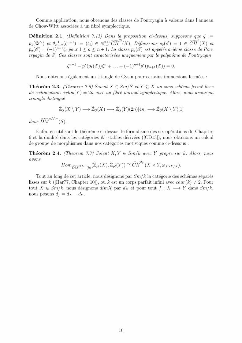
Comme application, nous obtenons des classes de Pontryagin a valeurs dans l’anneaude Chow-WItt associees a un fibre symplectique.
Definition 2.1. (Definition 7.11) Dans la proposition ci-dessus, supposons que ζ :=
p1(U∨) et θ−1
2n+2(ζn+1) := (ζi) ∈ ⊕
n+1i=1 CH
2i(X). Definissons p0(E ) = 1 ∈ CH
0(X) et
pa(E ) = (−1)a−1ζi pour 1 ≤ a ≤ n+1. La classe pa(E ) est appelee a-ieme classe de Pon-tryagin de E . Ces classes sont caracterisees uniquement par le polynome de Pontryagin
ζn+1 − p∗(p1(E ))ζn + . . .+ (−1)n+1p∗(pn+1(E )) = 0.
Nous obtenons egalement un triangle de Gysin pour certains immersions fermees :
Theorem 2.3. (Theorem 7.6) Soient X ∈ Sm/S et Y ⊆ X un sous-schema ferme lissede codimension codim(Y ) = 2n avec un fibre normal symplectique. Alors, nous avons untriangle distingue
ZS(X \ Y ) −→ ZS(X) −→ ZS(Y )(2n)[4n] −→ ZS(X \ Y )[1]
dans DMeff,−
(S).
Enfin, en utilisant le theoreme ci-dessus, le formalisme des six operations du Chapitre6 et la dualite dans les categories A1-stables derivees ([CD13]), nous obtenons un calculde groupe de morphismes dans nos categories motiviques comme ci-dessous :
Theorem 2.4. (Theorem 7.7) Soient X, Y ∈ Sm/k avec Y propre sur k. Alors, nousavons
HomDM
eff,−(k)(Zpt(X), Zpt(Y )) ∼= CH
dY(X × Y, ωX×Y/X).
Tout au long de cet article, nous designons par Sm/k la categorie des schemas separeslisses sur k ([Har77, Chapter 10]), ou k est un corps parfait infini avec char(k) 6= 2. Pourtout X ∈ Sm/k, nous designons dimX par dX et pour tout f : X −→ Y dans Sm/k,nous posons df = dX − dY .
10

Chapter 3
Virtual Objects and Their
Calculation
In this section we will introduce the category of virtual vector bundles and explain basictechniques of calculation. The definitions all come from [Del87, Section 4], but we recallthem here for clarity.
Definition 3.1. ([Del87, 4.1]) A category C is called a commutative Picard category if
1. All morphisms are isomorphisms.
2. There is a bifunctorial pairing
+ : C × C −→ C
satisfying
(a) For every x, y, z ∈ C , an associativity isomorphism
a(x, y, z) : (x+ y) + z −→ x+ (y + z);
(b) For every x, y ∈ C , a commutativity isomorphism
c(x, y) : x+ y −→ y + x.
Furthermore, they satisfy associativity and commutativity constraints ([Mac63]).
3. For every P ∈ C , the functors X 7−→ P +X and X 7−→ X + P are equivalences ofcategories. Thus there is a unit element 0 such that 0 +X ∼= X for every X ∈ C ,and there is an object −X ∈ C such that X + (−X) ∼= 0.
Definition 3.2. Let X be a scheme. Define V ect(X) to be the category of vector bundlesover X. Denote by (V ect(X), iso) the subcategory of V ect(X) with the same objects butpicking only isomorphisms as morphisms.
Definition 3.3. ([Del87, 4.3]) Let C be a commutative Picard category and let X be ascheme. A bracket functor on X (with coefficients in C ) is a covariant functor
[−] : (V ect(X), iso) −→ C
such that:
11

1. For any exact sequence of vector bundles
0 −→ E1 −→ E2 −→ E3 −→ 0,
there is an isomorphism Σ : [E2] −→ [E1] + [E3] being natural with respect toismorphisms between exact sequences.
2. There is an isomophism z : [0] −→ 0 such that for every E ∈ V ect(X), the composite
[E] Σ // [0] + [E] z // 0 + [E] // [E]
is id[E].
3. (Remark 3.1) For every consecutive subbundle inclusions E1 ⊆ E2 ⊆ E3, there is acommutative diagram
[E3]Σ //
Σ
[E1] + [E3/E1]
Σ
[E2] + [E3/E2]Σ // [E1] + [E2/E1] + [E3/E2].
4. For every E1, E2, there is a commutative diagram
[E1 ⊕ E2]Σ //
Σ
[E1] + [E2]
c(E1,E2)ww
[E2] + [E1].
The following comes from [Del87, 4.3]:
Proposition 3.1. Let X be a scheme. There is a commutative Picard category V (V ect(X))with a bracket functor on X such that for every commutative Picard category C with abracket functor on X, there is a unique additive functor F : V (V ect(X)) −→ C makingthe following diagram commute
(V ect(X), iso)[−]
//
[−]
V (V ect(X))F
vvC .
The category V (V ect(X)) is called the category of virtual vector bundles over X.
For convenience, we will still denote [E] by E in the sequel. The following propositionstrengthens Definition 3.3, (4) a little bit.
Proposition 3.2. Suppose we have a commutative diagram of vector bundles over X withexact row and column
0
D
d
∼=v
0 // Aa //
∼=
u
Bb
//
c
C // 0
E
0.
12

Then the following diagram commutes in V (V ect(X))
B //
A+ C
c(E,D)(u+v−1)yy
D + E.
Proof. Since v−1b splits d, it’s a standard argument that there exists a unique ξ : E −→ Bsuch that
ξ c = idB − d v−1 b, c ξ = idE.
So we have commutative diagrams with exact rows:
0 // Di1 // D ⊕ E
p2//
d+ξ
E // 0
0 // Dd // B
c // E // 0
0 // Ei2 //
u−1
D ⊕ Ep1
//
d+ξ
D //
v
0
0 // Aa // B
b // C // 0.
Hence the statement follows from the commutative diagram of Definition 3.3, (4):
A+ C
B
44
//
(d+ξ)−1##
D + Ec(D,E)
// E +D
u−1+v
OO
D ⊕ E.
OO 99
The next theorem is a fundamental tool for calculations in virtual vector bundles.
Theorem 3.1. 1. Suppose we have a commutative diagram of vector bundles over Xwith exact rows and columns
0
0
K
K
0 // V1 //
V2
// C // 0
0 //W1//
W2//
C // 0
0 0.
Then we have a commutative diagram in V (V ect(X))
V2 //
K +W2
V1 + C // K +W1 + C.
13

2. Suppose we have a commutative diagram of vector bundles over X with exact rowsand columns
0
0
0 // V1 //
V2
// C // 0
0 //W1//
W2//
C // 0
D
D
0 0.
Then we have a commutative diagram in V (V ect(X))
W2//
V2 +D // V1 + C +D
c(C,D)
ww
W1 + C
V1 +D + C.
3. Suppose we have a commutative diagram of vector bundles over X with exact rowsand columns
0
0
K
K
0 // T // V1
// V2 //
0
0 // T //W1//
W2//
0
0 0.
Then we have a commutative diagram in V (V ect(X))
V1 //
T + V2 // T +K +W2
c(T,K)
ww
K +W1
K + T +W2.
4. Suppose we have a commutative diagram of vector bundles over X with exact rows
14

and columns0
0
0 // K // V1
// V2 //
0
0 // K //W1//
W2//
0
C
C
0 0.
Then we have a commutative diagram in V (V ect(X))
W1//
K +W2
V1 + C // K + V2 + C.
Proof. 1. We have injections K −→ V1 −→ V2, which gives the diagram by Definition3.3, (3).
2. We have injections V1 −→ V2 −→ W2 and V1 −→ W1 −→ W2. These give twocommutative diagrams by Definition 3.3, (3)
W2//
V1 +W2/V1
Σ1
V2 +D // V1 + C +D
W2//
V1 +W2/V1
Σ2
W1 + C // V1 +D + C
.
Moreover, we have a commutative diagram with exact row and column
Σ2 : 0
D
Σ1 : 0 // C //W2/V1 //
D // 0
C
0
.
Thus we have a commutative diagram
W2/V1Σ1 //
Σ2 %%
C +D
c(C,D)
D + C
by Proposition 3.2. So combining the diagrams above gives the result.
15
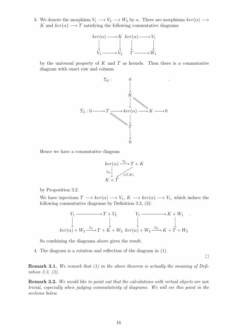
3. We denote the morphism V1 −→ V2 −→ W2 by α. There are morphisms ker(α) −→K and ker(α) −→ T satisfying the following commutative diagrams
ker(α) //
K
V1 // V2
ker(α) //
V1
T //W1
by the universal property of K and T as kernels. Then there is a commutativediagram with exact row and column
Σ2 : 0
K
Σ1 : 0 // T // ker(α) //
K // 0
T
0
.
Hence we have a commutative diagram
ker(α)Σ1 //
Σ2
T +K
c(T,K)yy
K + T
by Proposition 3.2.
We have injections T −→ ker(α) −→ V1, K −→ ker(α) −→ V1, which induce thefollowing commutative diagrams by Definition 3.3, (3):
V1 //
T + V2
ker(α) +W2Σ1 // T +K +W2
V1 //
K +W1
ker(α) +W2Σ2 // K + T +W2
.
So combining the diagrams above gives the result.
4. The diagram is a rotation and reflection of the diagram in (1).
Remark 3.1. We remark that (1) in the above theorem is actually the meaning of Defi-nition 3.3, (3).
Remark 3.2. We would like to point out that the calculations with virtual objects are nottrivial, especially when judging commutativity of diagrams. We will see this point in thesections below.
16

Chapter 4
Correspondences from an Axiomatic
Viewpoint
In this section, we are going to axiomatize the notion of correspondences, using thelanguage of virtual vector bundles defined in the previous section. They are designedbasicly to comply with properties of Chow rings or Chow-Witt rings.
Definition 4.1. Let X be a noetherian scheme and i ∈ N. We denote by Zi(X) the setof closed subsets in X whose components are all of codimension i.
Definition 4.2. Let X ∈ Sm/k, C ∈ Zi(X) and D ∈ Zj(X). We say that C and Dintersect properly if C ∩D ∈ Zi+j(X).
We now start our list of axioms.
Axiom 1. (Twists) For every X ∈ Sm/k, we have a commutative Picard category (Defi-nition 3.1) PX with an additive functor pX : V (V ect(X)) −→PX and a rank morphismrkX : PX −→ F(F = 0 or Z/2Z) such that:
1. The following diagram commutes
V (V ect(X))rkX //
pY
Z
PXrkX // F,
where the upper horizontal arrow is defined by rkX([E]) = rk(E).
2. For every f : X −→ Y in Sm/k, there is a pull-back morphism f ∗ : PY −→ PX
such that the following diagrams commute
PYf∗
//
rkY
PX
rkX||
F
V (V ect(Y ))f∗
//
pY
V (V ect(X))
pX
PYf∗
// PX ,
where f ∗ : V (V ect(Y )) −→ V (V ect(X)) is defined by f ∗([E]) = [f ∗E]. We havef ∗g∗ = (g f)∗ for any morphisms f, g in Sm/k and f ∗(−v) = −f ∗(v).
Remark 4.1. In practice, the categories PX should be chosen as “small” as possible.Since this will allow more isomophisms, such as orientations, as we will see in Definition7.19.
17

Axiom 2. (Correspondences) For every X ∈ Sm/k, i ∈ N, C ∈ Zi(X) and v ∈PX , thereexists an abelian group Ei
C(X, v) which is called the group of correspondences supportedon C with twist v. These groups are functorial with respect to v. Moreover, if C = ∅,then Ei
C(X, v) = 0.
We are now going to describe further properties that these groups should satisfy.
Axiom 3. (Extension of Supports) For every X ∈ Sm/k, C1 ⊆ C2 ∈ Zi(X), i ∈ N,v ∈PX , we have an injective morphism
e(C1, C2) : EiC1(X, v) −→ Ei
C2(X, v)
which is called the extension of support. This map is functorial with respect to v.For any disjoint C1, C2 ∈ Z
i(X), we have
EiC1∪C2
(X, v) ∼= EiC1(X, v)⊕ Ei
C2(X, v)
via extension of supports. Moreover, for any C1 ⊆ C2 ⊆ C3 we have
e(C2, C3) e(C1, C2) = e(C1, C3).
Axiom 4. (Products) Suppose X ∈ Sm/k, v1, v2 ∈ PX , C1, C2 ∈ Zi(X) and i, j ∈ N.
Suppose C1 and C2 intersect properly, then we have a product
EiC1(X, v1)× E
jC2(X, v2)
· // Ei+jC1∩C2
(X, v1 + v2) ,
This product is functorial with respect to twists and extension of supports.
Axiom 5. (Associativity) For any X ∈ Sm/k, va ∈ PX and Ca ∈ Zia(X), a = 1, 2, 3,
with pairwise proper intersections the following diagram commutes
Ei1C1(X, v1)× E
i2C2(X, v2)× E
i3C3(X, v3)
·×id
id×·// Ei1
C1(X, v1)× E
i2+i3C2∩C3
(X, v2 + v3)
·
Ei1+i2C1∩C2
(X, v1 + v2)× Ei3C3(X, v3)
·
Ei1+i2+i3C1∩C2∩C3
(X, v1 + (v2 + v3))a(v1,v2,v3)−1
rr
Ei1+i2+i3C1∩C2∩C3
(X, (v1 + v2) + v3).
Axiom 6. (Conditional Commutativity) Let X ∈ Sm/k, Ca ∈ Zia(X), ia ∈ N, va ∈PX
where a = 1, 2. If (i1 + rkX(v1))(i2 + rkX(v2)) = 0 ∈ F and C1 and C2 intersect properly,the following diagram commutes:
Ei1C1(X, v1)× E
i2C2(X, v2)
· //
Ei1+i2C1∩C2
(X, v1 + v2)
c(v1,v2)
Ei2C2(X, v2)× E
i1C1(X, v1)
· // Ei1+i2C1∩C2
(X, v2 + v1).
Axiom 7. (Identity) For any X ∈ Sm/k, there is an element e in E0X(X, 0) such that
for any v ∈PX , i ∈ N and C ∈ Zi(X), the following diagrams commute
EiC(X, v)
e· // EiC(X, 0 + v)
u
ww
EiC(X, v)
EiC(X, v)
·e // EiC(X, v + 0)
u
ww
EiC(X, v),
where u are the unit constraints in PX . We call e the identity and denote it by 1.
18

Axiom 8. (Pull-Backs) Suppose f : X −→ Y is morphism in Sm/k, i ∈ N, C ∈ Zi(Y ),f−1(C) ∈ Zi(X) and v ∈PY . Then we have a pull-back morphism
EiC(Y, v) −→ Ei
f−1(C)(X, f∗v).
This morphism is functorial with respect to v and extension of supports.
Axiom 9. (Functoriality of Pull-Backs) Let Xg
// Yf
// Z be morphisms in Sm/k,i ∈ N, C ∈ Zi(Z), f−1(C) ∈ Zi(Y ), g−1f−1(C) ∈ Zi(X) and v ∈PZ. We have
(f g)∗ = g∗ f ∗.
The pull-back of the identity morphism is just the identity morphism.
Axiom 10. (Compability of Pull-Backs) Suppose that f : X −→ Y is a morphism inSm/k, and that C1 ∈ Zi(Y ) and C2 ∈ Zj(Y ) intersect properly for some i, j ∈ N (thesame for their preimages). For any v1, v2 ∈PY , we have a commutative diagram
EiC1(Y, v1)× E
jC2(Y, v2)
· //
f∗×f∗
Ei+jC1∩C2
(Y, v1 + v2)
f∗
Eif−1(C1)
(X, f ∗(v1))× Ejf−1(C2)
(X, f ∗(v2))· // Ei+j
f−1(C1∩C2)(X, f ∗(v1 + v2))
.
We always have f ∗(1) = 1.
Before proceeding further, we now recall some facts about tangent bundles and normalbundles.
Lemma 4.1. Let Xf
// Yg
// Z be morphisms in Sm/k.
1. If f , g are smooth, we have an exact sequence
0 −→ TX/Y −→ TX/Z −→ f ∗TY/Z −→ 0.
2. If f is a closed immersion and g, g f are smooth, we have an exact sequence
0 −→ TX/Z −→ f ∗TY/Z −→ NX/Y −→ 0.
3. If g is smooth and f , g f are closed immersions, we have an exact sequence
0 −→ f ∗TY/Z −→ NX/Y −→ NX/Z −→ 0.
4. If f , g are closed immersions, we have an exact sequence
0 −→ NX/Y −→ NX/Z −→ f ∗NY/Z −→ 0.
Proof. See [Har77, Chapter II, Proposition 8.11, Proposition 8.12 and Theorem 8.17 andChapter III, Proposition 10.4].
Lemma 4.2. Suppose that we have a Cartesian square of schemes
X ′ v //
g
X
f
Y ′ u // Y.
Then, the composite TX′/Y ′ −→ TX′/Y −→ v∗TX/Y is an isomorphism.
19

Proof. See [Har77, Chapter II, Proposition 8.10].
Lemma 4.3. Suppose that we have a Cartesian square in Sm/k
X ′ v //
g
X
f
Y ′ u // Y
such that f is a closed immersion. If one of the following conditions holds:
1. u is smooth,
2. u is a closed immersion and dimX ′ − dimY ′ = dimX − dimY ,
then the natural morphism γ defined by the following commutative diagram with exactrows
0 // v∗TX/k // v∗f ∗TY/k // v∗NX/Y// 0
0 // TX′/k//
α
OO
g∗TY ′/k//
β
OO
NX′/Y ′//
γ
OO
0
is an isomorphism.
Proof. If u is smooth, then α and β are surjective and have the same kernel by the previoustwo lemmas. So γ is an isomorphism by the snake lemma.
In the other case, the dimension condition implies NX′/Y ′ and NX/Y have the samerank. So we only have to prove γ∨ is surjective. We can assume that all schemes are affine.Suppose that Y = Spec(A), X = Spec(A/I), Y ′ = Spec(A/J) and X ′ = Spec(A/(I+J)).Then N∨
X/Y = I/I2 and N∨X′/Y ′ = (I + J)/(I2 + J) and the morphism γ is given by
I/I2 ⊗A/I A/(I + J) −→ (I + J)/(I2 + J)(i , a) 7−→ ai.
This is obviously surjective.
Axiom 11. (Push-Forwards for Smooth Morphisms) Suppose that f : X −→ Y is asmooth morphism in Sm/k, that n ∈ N, v ∈ PX and that C ∈ Zn+df (X) is finite overY . Then we have a morphism
f∗ : En+dfC (X, f ∗v − TX/Y ) −→ En
f(C)(Y, v),
which is functorial with respect to v and the extension of supports. The push-forward ofthe identity morphism is just the identity morphism (using TX/Y = 0).
We may also use the simplified notation
f ∗v − TX/Y −→ v
to denote f∗. Moreover, we can consider push-forwards of the form
f∗ : En+dfC (X, f ∗v1 − TX/Y + f ∗v2) −→ En
f(C)(Y, v1 + v2)
which are defined by the composite of the push-forward defined above and the commuta-tivity isomorphism c(−TX/Y , f
∗v2).
20

Axiom 12. (Functoriality of Push-Forwards for Smooth Morphisms) Suppose that Xg
// Yf
// Zare smooth morphisms in Sm/k, and that C ∈ Zi+dX−dZ (X) is finite over Z (i ∈ N). Sup-pose moreover that v ∈PZ. Then we have a commutative diagram
Ei+dX−dZC (X, (f g)∗v − TX/Z)
ϕ//
(fg)∗
((
Ei+dX−dZC (X, (f g)∗v − g∗TY/Z − TX/Y )
g∗
Ei+dY −dZg(C) (Y, f ∗v − TY/Z)
f∗
Eif(g(C))(Z, v)
where ϕ is obtained via the following composite
(f g)∗v − TX/Z −→ (f g)∗v − (TX/Y + g∗TY/Z)
−→ (f g)∗v − g∗TY/Z − TX/Y .
Axiom 13. (Push-Forward for Closed Immersions) Suppose f : X −→ Y is a closedimmersion in Sm/k, v ∈PY and C ∈ Zn+df (X). Then we have an isomorphism
f∗ : En+dfC (X,NX/Y + f ∗v) −→ En
f(C)(Y, v),
This morphism is also functorial in v and under extension of supports. The push-forwardof the identity is just the identity, by using NX/Y = 0.
So given a vector bundle V overX, the definition above gives an isomorphism EnC(X, V ) ∼=
En+rkX(V )C (V, 0) (Chapter 1) via the push-forward of the zero section.We may also use the simplified notation
NX/Y + f ∗v −→ v
to denote f∗. Moreover, we could also consider push-forwards of the form
f∗ : En+dfC (X, f ∗v1 +NX/Y + f ∗v2) −→ En
f(C)(Y, v1 + v2)
which are defined by the composite of the push-forward defined above and the commuta-tivity isomorphism c(f ∗v1, NX/Y ).
Axiom 14. (Functoriality Push-Forwards for Closed Immersions) Suppose that Xg
// Yf
// Zare closed immersions in Sm/k, C ∈ Zi+dX−dZ (X) and v ∈ PZ. Then we have a com-mutative diagram
Ei+dX−dZC (X,NX/Z + (f g)∗v)
ϕ//
(fg)∗
((
Ei+dX−dZC (X,NX/Y + g∗NY/Z + (f g)∗v)
g∗
Ei+dY −dZg(C) (Y,NY/Z + f ∗v)
f∗
Eif(g(C))(Z, v),
where ϕ is induced by the isomorphism NX/Z + (f g)∗v ∼= NX/Y + g∗NY/Z + (f g)∗v.
21

Axiom 15. (Base Change for Smooth Morphisms) Suppose we have a Cartesian squareof smooth schemes
X ′ v //
g
X
f
Y ′ u // Y
with f smooth. Let moreover c = dX − dY = dX′ − dY ′, n ∈ N, s ∈ PY , C ∈ Zn+c(X)
finite over Y such that v−1(C) ∈ Zn+c(X). Then the following diagram commutes
En+cC (X, f ∗s− TX/Y )
f∗//
v∗
Enf(C)(Y, s)
u∗
En+cv−1(C)(X
′, v∗f ∗s− v∗TX/Y )g∗
// Eng(v−1(C))(Y
′, u∗s).
Here we have used the canonical isomorphism TX′/Y ′ −→ v∗TX/Y of Lemma 4.2.
Axiom 16. (Base Change for Closed Immersions) Suppose that we have a Cartesiansquare of smooth schemes
X ′ v //
g
X
f
Y ′ u // Y
with f a closed immersion. Let c = dX − dY = dX′ − dY ′, s ∈ PY , C ∈ Zn+c(X) such
that v−1(C) ∈ Zn+c(X). Then the following diagram commutes
En+cC (X,NX/Y + f ∗s)
f∗//
v∗
Enf(C)(Y, s)
u∗
En+cv−1(C)(X
′, v∗NX/Y + v∗f ∗s)g∗
// Eng(v−1(C))(Y
′, u∗s).
Axiom 17. (Projection Formula for Smooth Morphisms) Suppose that we have a smoothmorphism f : X −→ Y in Sm/k and that n,m ∈ N. Let further C ∈ Zn+df (X) be finiteover Y and D ∈ Zm(Y ) be such that C and f−1(D) intersect properly and v1, v2 ∈ PY .Then the diagrams
En+dfC (X, f ∗v1 − TX/Y )× E
mD (Y, v2)
id×f∗//
f∗×id
En+dfC (X, f ∗v1 − TX/Y )× E
mf−1(D)(X, f
∗v2)
·
EnC(Y, v1)× E
mD (Y, v2)
·
En+m+dfC∩f−1(D)(X, f
∗v1 − TX/Y + f ∗v2)
f∗rr
En+mY,f(C)∩D(v1 + v2)
and
EmD (Y, v2)× E
n+dfC (X, f ∗v1 − TX/Y )
f∗×id//
id×f∗
Emf−1(D)(X, f
∗v2)× En+dfC (X, f ∗v1 − TX/Y )
·
EmD (Y, v2)× E
nC(Y, v1)
·
En+m+dfC∩f−1(D)(X, f
∗v2 + f ∗v1 − TX/Y )
f∗rr
En+mf(C)∩D(Y, v2 + v1)
22

commute.
Axiom 18. (Projection Formula for Closed Immersions) Suppose that we have a closedimmersion f : X −→ Y in Sm/k. Let n,m ∈ N, C ∈ Zn+df (X) and D ∈ Zm(Y ) besuch that f−1(D) ∈ Zm(X), and such that C and f−1(D) intersect properly. Let furtherv1, v2 ∈PY . Then the diagrams
En+dfC (X,NX/Y + f ∗v1)× E
mD (Y, v2)
id×f∗//
f∗×id
En+dfC (X,NX/Y + f ∗v1)× E
mf−1(D)(X, f
∗v2)
·
EnC(Y, v1)× E
mD (Y, v2)
·
En+m+dfC∩f−1(D)(X,NX/Y + f ∗v1 + f ∗v2)
f∗rr
En+mf(C)∩D(Y, v1 + v2)
and
EmD (Y, v2)× E
n+dfC (X,NX/Y + f ∗v1)
f∗×id//
id×f∗
Emf−1(D)(X, f
∗v2)× En+dfC (X,NX/Y + f ∗v1)
·
EmD (Y, v2)× E
nC(Y, v1)
·
En+m+dfC∩f−1(D)(X, f
∗v2 +NX/Y + f ∗v1)
f∗rr
En+mf(C)∩D(Y, v2 + v1)
commute.
We still need a compability between the two push-forwards introduced above.
Axiom 19. (Compability between Two Push-Forwards)
1. Suppose that Xf
// Zg
// Y are morphisms in Sm/k, that f is a closed immer-sion and that g, g f are smooth. Let C ∈ Zi+dX−dY (X) be finite over Y , i ∈ N andv ∈PY . Then the following diagram commutes
Ei+dX−dYC (X,NX/Z + f ∗g∗v − f ∗TZ/Y )
f∗
c(NX/Z ,f∗g∗v)// Ei+dX−dY
C (X, f ∗g∗v +NX/Z − f∗TZ/Y )
ϕ
Ei+dZ−dYf(C) (Z, g∗v − TZ/Y )
g∗
Ei+dX−dYC (X, f ∗g∗v − TX/Y )
(gf)∗
rr
Eig(f(C))(Y, v),
,
where ϕ is induced by Lemma 4.1, (2).
2. Suppose that Xf
// Zg
// Y are morphisms in Sm/k with g smooth and f , g fclosed immersions. Let C ∈ Zi+dX−dY (X) be finite over Y , i ∈ N and v ∈ PY .
23
Then the following diagram commutes
Ei+dX−dYC (X,NX/Z + f ∗g∗v − f ∗TZ/Y )
f∗
c(NX/Z+f∗g∗v,−f∗TZ/Y )// Ei+dX−dY
C (X,−f ∗TZ/Y +NX/Z + f ∗g∗v)
ϕ
Ei+dZ−dYf(C) (Z, g∗v − TZ/Y )
g∗
Ei+dX−dYC (X,NX/Y + f ∗g∗v)
(gf)∗
rr
Eig(f(C))(Y, v),
where ϕ is induced by Lemma 4.1, (3).
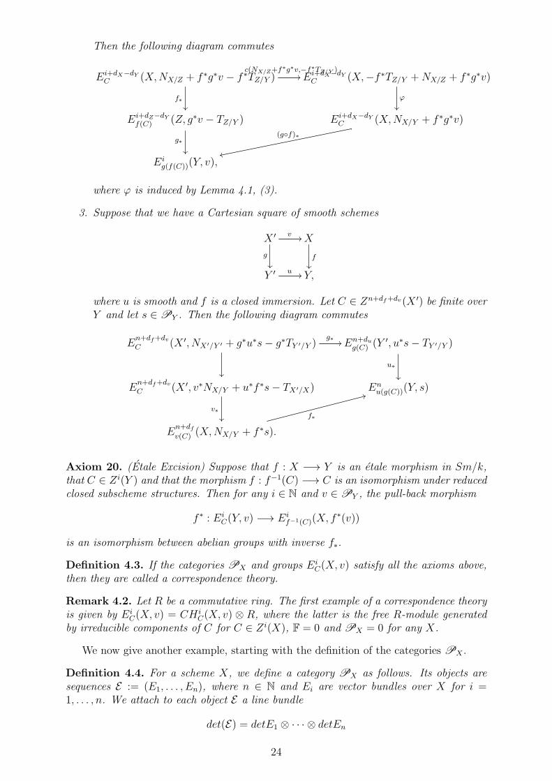
3. Suppose that we have a Cartesian square of smooth schemes
X ′ v //
g
X
f
Y ′ u // Y,
where u is smooth and f is a closed immersion. Let C ∈ Zn+df+dv(X ′) be finite overY and let s ∈PY . Then the following diagram commutes
En+df+dvC (X ′, NX′/Y ′ + g∗u∗s− g∗TY ′/Y )
g∗//
En+dug(C) (Y
′, u∗s− TY ′/Y )
u∗
En+df+dvC (X ′, v∗NX/Y + u∗f ∗s− TX′/X)
v∗
Enu(g(C))(Y, s)
En+dfv(C) (X,NX/Y + f ∗s).
f∗
33
Axiom 20. (Etale Excision) Suppose that f : X −→ Y is an etale morphism in Sm/k,that C ∈ Zi(Y ) and that the morphism f : f−1(C) −→ C is an isomorphism under reducedclosed subscheme structures. Then for any i ∈ N and v ∈PY , the pull-back morphism
f ∗ : EiC(Y, v) −→ Ei
f−1(C)(X, f∗(v))
is an isomorphism between abelian groups with inverse f∗.
Definition 4.3. If the categories PX and groups EiC(X, v) satisfy all the axioms above,
then they are called a correspondence theory.
Remark 4.2. Let R be a commutative ring. The first example of a correspondence theoryis given by Ei
C(X, v) = CH iC(X, v) ⊗ R, where the latter is the free R-module generated
by irreducible components of C for C ∈ Zi(X), F = 0 and PX = 0 for any X.
We now give another example, starting with the definition of the categories PX .
Definition 4.4. For a scheme X, we define a category PX as follows. Its objects aresequences E := (E1, . . . , En), where n ∈ N and Ei are vector bundles over X for i =1, . . . , n. We attach to each object E a line bundle
det(E) = detE1 ⊗ · · · ⊗ detEn
24

and an integerrk(E) = rkE1 + · · ·+ rkEn ∈ Z/2Z.
The morphisms between objects E = (E1, . . . , En) and F = (F1, . . . , Fm) are given by
HomPX(E ,F) =
IsomOX
(det(E), det(F)) if rk(E) = rk(F).
∅ else.
The composition law is inherited from the category of line bundles.
Remark 4.3. The category PX is equivalent to the category of Z/2Z-graded line bundlesconsidered in [Del87, 4.3]. However, the category PX will be more convenient in ourcomputations.
To complete the definition of our correspondence theory, we set
CHi
C(X, v) = CHi
C(X, det(v)).
for every X ∈ Sm/k, C ∈ Zi(X), v ∈PX . These are precisely the MW-correspondencesdefined in [CF14]. We will give a plan of proof of the following theorem in Chapter 8.
Theorem 4.1. The collection of MW-correspondences form a correspondence theory withtwists in PX .
25

Chapter 5
Sheaves with E-Tranfers and Their
Operations
In this section, we develop the theory of sheaves with E-transfers over a smooth base asin [D07] and [CF14], where E is a correspondence theory.
Since there will be heavy calculations involving twists, we use the abbreviation (α, v)for α ∈ Ei
C(X, v) from now on for convenience and clarity. We extend this notation tooperations such as (α, v) · (β, u), f ∗((α, v)). For S ∈ Sm/k, we denote the category ofsmooth schemes over S by Sm/S.
We will need the notion of admissible subset coming from [CF14, Definition 4.1].
Definition 5.1. Let X, Y ∈ Sm/S. We denote by AS(X, Y ) the set of closed subsetsT of X ×S Y whose components are all finite over X and of dimension dim(X). Theelements of AS(X, Y ) are called admissible subsets from X to Y over S.
Lemma 5.1. In the definition above, T itself is also finite over X.
Proof. For every affine open subset U of X, T ∩ U is affine since each of its componentsare affine (see [Har77, Chapter III, Exercises 3.2]). Its structure ring is a submodule of afinite OX(U)-module. Hence we conclude that T ∩ U is finite over U .
Definition 5.2. Let S ∈ Sm/k, and let X, Y ∈ Sm/S. The group
CorS(X, Y ) = lim−→T∈AS(X,Y )
EdY −dST (X ×S Y,−TX×SY/X)
is called the group of finite E-correspondences between X and Y over S.
We can now consider the category CorS(X, Y ), whose objects are smooth schemes
over S and morphisms between X and Y are just CorS(X, Y ) defined above. Our aim isnow to study the composition in that category.
To avoid complicated expressions, we denote for smooth schemes X, Y and Z thescheme X ×S Y ×S Z by XY Z and the projection X ×S Y ×S Z −→ Y ×S Z by pXY ZY Z .We extend this notation to arbitrary products of schemes in an obvious way.
Given any α ∈ CorS(X, Y ) and β ∈ CorS(Y, Z), we may suppose they are definedover admissible subsets. With this in mind, the image of
pXY ZXZ∗ (pXY Z∗Y Z ((β,−TY Z/Y )) · p
XY Z∗XY ((α,−TXY/X)))
in CorS(X,Z) is just defined as β α. It is straightforward to check that this definitionis compatible with extension of supports.
Proposition 5.1. The composition law defined above is associative.
26

Proof. Suppose that X α // Yβ
// Zγ
//W are morphisms in CorS. As before, wemay suppose that each correspondence is defined over an admissible subset.
Consider the Cartesian squares
XY ZW //
XZW
XY Z // XZ
XY ZW //
XYW
Y ZW // YW.
Now
γ (β α)
=pXZWXW∗ (pXZW∗ZW ((γ,−TZW/Z))p
XZW∗XZ pXY ZXZ∗ (p
XY Z∗Y Z ((β,−TY Z/Y ))p
XY Z∗XY ((α,−TXY/X))))
by definition
=pXZWXW∗ (pXZW∗ZW (γ)pXZW∗
XZ pXY ZXZ∗ ((pXY Z∗Y Z (β)pXY Z∗XY (α),−TXY Z/XY − TXY Z/XZ)))
by definition of the product
=pXZWXW∗ (pXZW∗ZW (γ)pXY ZWXZW∗ p
XY ZW∗XY Z ((pXY Z∗Y Z (β)pXY Z∗XY (α),−TXY Z/XY − TXY Z/XZ)))
by Axiom 15 for the left square above
=pXZWXW∗ (pXZW∗ZW (γ)pXY ZWXZW∗ (p
XY ZW∗Y Z (β)pXY ZW∗
XY (α),−TXY ZW/XYW − TXY ZW/XZW ))
by Axiom 9 and Axiom 10
=pXZWXW∗ pXY ZWXZW∗ ((p
XY ZW∗ZW (γ),−TXY ZW/XY Z)p
XY ZW∗Y Z (β)pXY ZW∗
XY (α))
by Axiom 17 for pXY ZWXZW
=pXZWXW∗ pXY ZWXZW∗ ((δ,−p
XY ZW∗XW TXW/X − p
XY ZW∗XZW TXZW/XW − TXY ZW/XZW ))
by definition of the product where δ = pXY ZW∗ZW (γ)pXY ZW∗
Y Z (β)pXY ZW∗XY (α)
=pXY ZWXW∗ ((δ,−pXY ZW∗XW TXW/X − TXY ZW/XW ))
by Axiom 12
=pXYWXW∗ pXY ZWXYW∗ ((δ,−p
XY ZW∗XW TXW/X − p
XY ZW∗XYW TXYW/XW − TXY ZW/XYW ))
by Axiom 12, note that we have used c(−TXY ZW/XYW ,−TXY ZW/XZW )
=pXYWXW∗ (pXY ZWXYW∗ (p
XY ZW∗ZW (γ)pXY ZW∗
Y Z (β))pXYW∗XY (α))
by Axiom 17 for pXY ZWXYW
=pXYWXW∗ (pXY ZWXYW∗ p
XY ZW∗Y ZW (pY ZW∗
ZW (γ)(pY ZW∗Y Z (β),−TY ZW/YW ))pXYW∗
XY (α))
by Axiom 9 and Axiom 10
=pXYWXW∗ (pXYW∗YW pY ZWYW∗ (p
Y ZW∗ZW (γ)pY ZW∗
Y Z (β))pXYW∗XY (α))
by Axiom 15 for the right square above
=(γ β) α
by definition.
Definition 5.3. Consider the functor
γ : Sm/S −→ CorS,
defined on objects by γ(X) = X. Given an S-morphism f : X −→ Y , we have the graphmorphism Γf : X −→ X ×S Y and the natural map
Γ∗fTX×SY/X −→ NX/X×SY
27
of Lemma 4.1 is an isomorphism. We set γ(f) to be image of the element 1 ∈ E0X(X, 0)
of Axiom 7 under the composite
E0X(X, 0)
// E0X(X,NX/X×SY − Γ∗
fTX×SY/X)Γf∗
// EdY −dSX (X ×S Y,−TX×SY/X)
CorS(X, Y ).
We prove in the next couple of results that γ respects the composition of both cate-gories, starting with some easy cases.
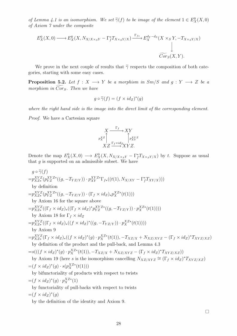
Proposition 5.2. Let f : X −→ Y be a morphism in Sm/S and g : Y −→ Z be a
morphism in CorS. Then we have
g γ(f) = (f × idZ)∗(g)
where the right hand side is the image into the direct limit of the corresponding element.
Proof. We have a Cartesian square
XΓf
// XY
XZ
pXZX
OO
Γf×idZ// XY Z.
pXY ZXY
OO
Denote the map E0X(X, 0) −→ E0
X(X,NX/X×SY − Γ∗fTX×SY/X) by t. Suppose as usual
that g is supported on an admissible subset. We have
g γ(f)
=pXY ZXZ∗ (pXY Z∗Y Z ((g,−TY Z/Y )) · p
XY Z∗XY Γf∗((t(1), NX/XY − Γ∗
fTXY/X)))
by definition
=pXY ZXZ∗ (pXY Z∗Y Z ((g,−TY Z/Y )) · (Γf × idZ)∗p
XZ∗X (t(1)))
by Axiom 16 for the square above
=pXY ZXZ∗ ((Γf × idZ)∗((Γf × idZ)∗pXY Z∗Y Z ((g,−TY Z/Y )) · p
XZ∗X (t(1))))
by Axiom 18 for Γf × idZ
=pXY ZXZ∗ ((Γf × idZ)∗((f × idZ)∗((g,−TY Z/Y )) · p
XZ∗X (t(1))))
by Axiom 9
=pXY ZXZ∗ (Γf × idZ)∗((f × idZ)∗(g) · pXZ∗X (t(1)),−TXZ/X +NXZ/XY Z − (Γf × idZ)
∗TXY Z/XZ)
by definition of the product and the pull-back, and Lemma 4.3
=s(((f × idZ)∗(g) · pXZ∗X (t(1)),−TXZ/X +NXZ/XY Z − (Γf × idZ)
∗TXY Z/XZ))
by Axiom 19 (here s is the isomorphism cancelling NXZ/XY Z∼= (Γf × idZ)
∗TXY Z/XZ)
=(f × idZ)∗(g) · s(pXZ∗X (t(1)))
by bifunctoriality of products with respect to twists
=(f × idZ)∗(g) · pXZ∗X (1)
by functoriality of pull-backs with respect to twists
=(f × idZ)∗(g)
by the definition of the identity and Axiom 9.
28

Proposition 5.3. Let f : X −→ Y be a morphism in CorS and let g : Y −→ Z be asmooth morphism in Sm/S. Let t be the composite
− TXY/X
−→− (idX × Γg)∗TXY Z/XY +NXY/XY Z − TXY/X
−→− (idX × Γg)∗TXY Z/XY +NXY/XY Z − (idX × Γg)
∗TXY Z/XZ
−→− (idX × Γg)∗TXY Z/XY +NXY/XY Z −NXY/XY Z − TXY/XZ
−→− (idX × Γg)∗TXY Z/XY − TXY/XZ
−→− (idX × g)∗TXZ/X − TXY/XZ .
Then we haveγ(g) f = (idX × g)∗(t(f)),
where the right side is the image into the direct limit of the corresponding element.
Proof. We have a Cartesian square
YΓg
// Y Z
XY
pXYY
OO
idX×Γg// XY Z,
pXY ZY Z
OO
an isomorphism s : 0 −→ NY/Y Z − Γ∗gTY Z/Y and an isomorphism
r : −TXY/X −→ NXY/XY Z − (idX × Γg)∗TXY Z/XY − TXY/X .
Suppose that f is supported on some admissible subset. We obtain
γ(g) f
=pXY ZXZ∗ (pXY Z∗Y Z Γg∗((s(1), NY/Y Z − Γ∗
gTY Z/Y )) · pXY Z∗XY ((f,−TXY/X))
by definition
=pXY ZXZ∗ ((idX × Γg)∗pXY ∗Y ((s(1), NY/Y Z − Γ∗
gTY Z/Y )) · pXY Z∗XY (f))
by Axiom 16 for the square above
=pXY ZXZ∗ (idX × Γg)∗(pXY ∗Y ((s(1), NY/Y Z − Γ∗
gTY Z/Y )) · (idX × Γg)∗pXY Z∗XY (f))
by Axiom 18 for idX × Γg
=pXY ZXZ∗ (idX × Γg)∗(r((idX × Γg)∗pXY Z∗XY (f)))
by functoriality of pull-backs and products with respect to twists
=(idX × g)∗(t((idX × Γg)∗pXY Z∗XY (f)))
by Axiom 19
=(idX × g)∗(t(f))
by Axiom 9.
Proposition 5.4. Let f : X −→ Y be a morphism in CorS and let g : Y −→ Z be aclosed immersion in Sm/S. Let t′ be the composite
− TXY/X
−→− TXY/X +NXY/XY Z − (idX × Γg)∗TXY Z/XY
−→− TXY/X + (idX × Γg)∗TXY Z/XZ +NXY/XZ − (idX × Γg)
∗TXY Z/XY
−→− TXY/X + TXY/X +NXY/XZ − (idX × Γg)∗TXY Z/XY
−→NXY/XZ − (idX × Γg)∗TXY Z/XY
−→NXY/XZ − (idX × g)∗TXZ/X .
29
Then we haveγ(g) f = (idX × g)∗(t
′(f)),
where the right side is the image into the direct limit of the corresponding element.
Proof. The same proof as in the above proposition applies.
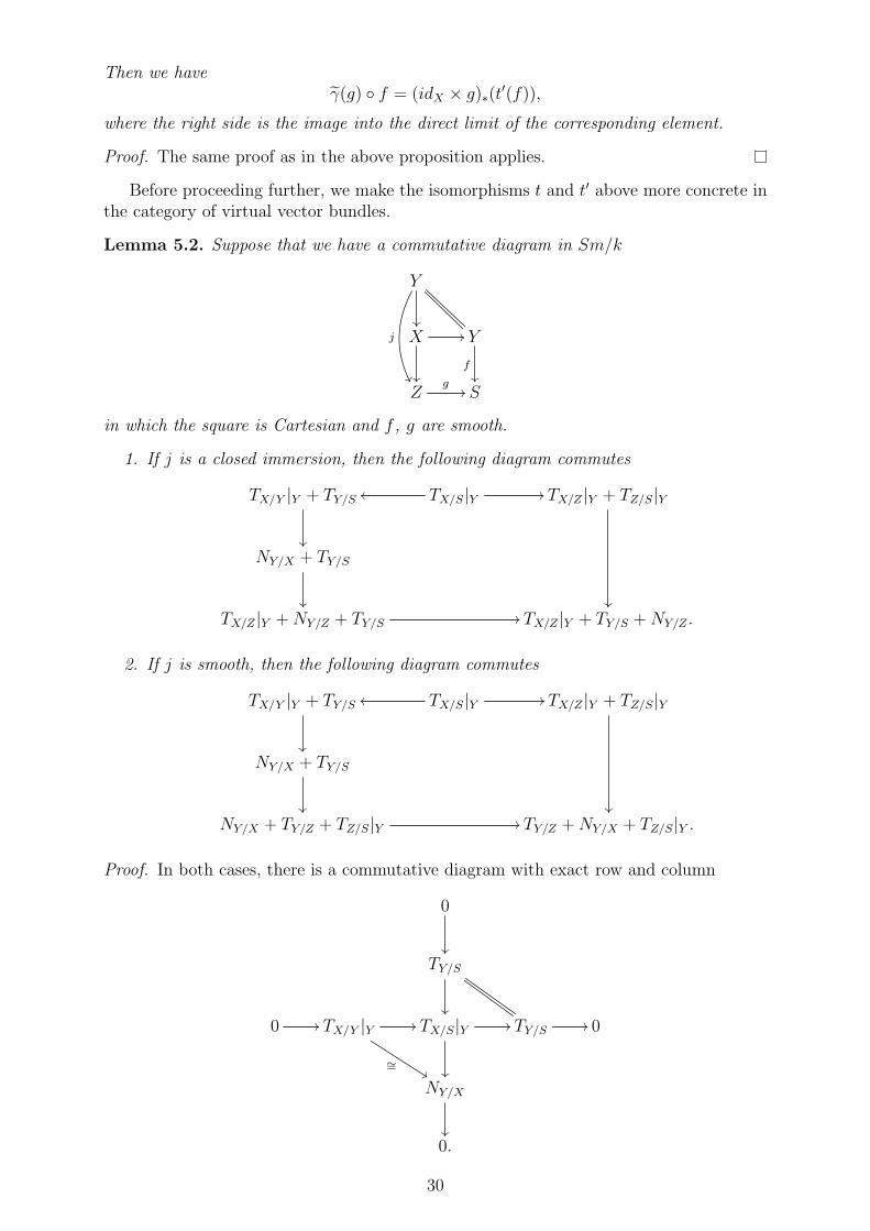
Before proceeding further, we make the isomorphisms t and t′ above more concrete inthe category of virtual vector bundles.
Lemma 5.2. Suppose that we have a commutative diagram in Sm/k
Y
j
X //
Y
f
Zg
// S
in which the square is Cartesian and f , g are smooth.
1. If j is a closed immersion, then the following diagram commutes
TX/Y |Y + TY/S
TX/S|Yoo // TX/Z |Y + TZ/S|Y
NY/X + TY/S
TX/Z |Y +NY/Z + TY/S // TX/Z |Y + TY/S +NY/Z .
2. If j is smooth, then the following diagram commutes
TX/Y |Y + TY/S
TX/S|Yoo // TX/Z |Y + TZ/S|Y
NY/X + TY/S
NY/X + TY/Z + TZ/S|Y // TY/Z +NY/X + TZ/S|Y .
Proof. In both cases, there is a commutative diagram with exact row and column
0
TY/S
0 // TX/Y |Y //
∼=%%
TX/S|Y //
TY/S // 0
NY/X
0.
30

It induces a commutative diagram
TX/S|Y //
TX/Y |Y + TY/S
vv
TY/S +NY/X
by Theorem 3.1, (3). We now pass to the proof of the first statement. We have acommutative diagram with exact columns and rows
0
0
TY/S
TY/S
0 // TX/Z |Y // TX/S|Y
// TZ/S|Y //
0
0 // TX/Z |Y // NY/X//
NY/Z//
0
0 0.
We deduce the following commutative diagram by Theorem 3.1, (3)
TX/S|Y //
TX/Z |Y + TZ/S|Y // TX/Z |Y + TY/S +NY/Z
tt
TY/S +NY/X
TY/S + TX/Z |Y +NY/Z .
Furthermore, there is an obvious commutative diagram
NY/X + TY/S
TY/S +NY/X//oo TY/S + TX/Z |Y +NY/Z
TX/Z |Y +NY/Z + TY/S // TX/Z |Y + TY/S +NY/Z
.
So the statement follows by combining the diagrams above.For the second statement, observe that we have a commutative diagram with exact
columns and rows
0
0
0 // TY/Z //
TY/S
// TZ/S|Y // 0
0 // TX/Z |Y //
TX/S|Y //
TZ/S|Y // 0
NY/X
NY/X
0 0.
31

Then the result follows by the same method as above by applying Theorem 3.1, (2) tothe diagram above.
Lemma 5.3. Suppose that X, Y, Z ∈ Sm/S and that g : Y −→ Z is a morphism inSm/S.
1. If g is a closed immersion, then the isomorphism t in Proposition 5.3 is equal to
−TXY/X −→ NXY/XZ −NXY/XZ − TXY/X −→ NXY/XZ − (idX × g)∗TXZ/X .
2. If g is smooth, then the isomorphism t′ in Proposition 5.4 is equal to
−TXY/X −→ −(idX × g)∗TXZ/X − TXY/XZ .
Proof. We have a commutative diagram in Sm/k
XY
idX×Γg
idX×g
XY ZpXY ZXY
//
pXY ZXZ
XY
pXYX
XZpXZX
// X
in which the square is Cartesian. Suppose first that g is a closed immersion. In that case,we show that the composite
− TXY/X
−→− TXY/X +NXY/XY Z − (idX × Γg)∗TXY Z/XY
−→− TXY/X + (idX × Γg)∗TXY Z/XZ +NXY/XZ − (idX × Γg)
∗TXY Z/XY
−→NXY/XZ − (idX × Γg)∗TXY Z/XY
−→NXY/XZ − (idX × g)∗TXZ/X
−→NXY/XZ −NXY/XZ − TXY/X
−→− TXY/X
is just id−TXY/X. Indeed, it is equal to
− TXY/X
−→− TXY/X +NXY/XY Z − (idX × Γg)∗TXY Z/XY
−→− TXY/X − (idX × Γg)∗TXY Z/XY +NXY/XY Z
−→− TXY/X − (idX × g)∗TXZ/X +NXY/XY Z
−→− TXY/X −NXY/XZ − TXY/X +NXY/XY Z
−→− TXY/X −NXY/XZ − TXY/X + (idX × Γg)∗TXY Z/XZ +NXY/XZ
−→−NXY/XZ − TXY/X +NXY/XZ
−→− TXY/X ,
where the sixth arrow is the cancellation map between the first and the fourth term. ByLemma 5.2, (1) and the commutative diagram above, we have a commutative diagram
(idX × Γg)∗TXY Z/XY + TXY/X
(idX × Γg)∗TXY Z/Xoo
NXY/XY Z + TXY/X
(idX × Γg)∗TXY Z/XZ + (idX × g)
∗TXZ/X
(idX × Γg)∗TXY Z/XZ +NXY/XZ + TXY/X // (idX × Γg)
∗TXY Z/XZ + TXY/X +NXY/XZ .
32

Hence the composite above is equal to
− TXY/X
−→− TXY/X +NXY/XY Z − (idX × Γg)∗TXY Z/XY
−→− TXY/X − (idX × Γg)∗TXY Z/XY +NXY/XY Z
−→− TXY/X −NXY/XY Z +NXY/XY Z
−→− TXY/X −NXY/XZ − (idX × Γg)∗TXY Z/XZ +NXY/XY Z
−→− TXY/X −NXY/XZ − (idX × Γg)∗TXY Z/XZ + (idX × Γg)
∗TXY Z/XZ +NXY/XZ
−→− TXY/X ,
which gives the result.Suppose next that g is smooth. We show that the composite
− TXY/X
−→− (idX × Γg)∗TXY Z/XY +NXY/XY Z − TXY/X
−→− (idX × Γg)∗TXY Z/XY +NXY/XY Z − (idX × Γg)
∗TXY Z/XZ
−→− (idX × Γg)∗TXY Z/XY +NXY/XY Z −NXY/XY Z − TXY/XZ
−→− (idX × Γg)∗TXY Z/XY − TXY/XZ
−→− (idX × g)∗TXZ/X − TXY/XZ
−→− TXY/X
is just id−TXY/X. By Lemma 5.2, (2) and the commutative diagram at the beginning of
the proof, we get a commutative diagram
(idX × Γg)∗TXY Z/XY + TXY/X
(idX × Γg)∗TXY Z/Xoo
NXY/XY Z + TXY/X
(idX × Γg)∗TXY Z/XZ + (idX × g)
∗TXZ/X
NXY/XY Z + TXY/XZ + (idX × g)∗TXZ/X // TXY/XZ +NXY/XY Z + (idX × g)
∗TXZ/X .
Hence the given composite is equal to
− TXY/X
−→− (idX × Γg)∗TXY Z/XY +NXY/XY Z − TXY/X
−→− (idX × Γg)∗TXY Z/XY − TXY/X +NXY/XY Z
−→−NXY/XY Z − TXY/X +NXY/XY Z
−→−NXY/XY Z − (idX × g)∗TXZ/X − TXY/XZ +NXY/XY Z
−→− (idX × g)∗TXZ/X − TXY/XZ
−→− TXY/X ,
where the fifth arrow is the cancellation between the first and the fourth term. The resultfollows.
Proposition 5.5. For any X ∈ Sm/S, γ(idX) is an identity. That is, for any X, Y ∈
Sm/S, f ∈ CorS(X, Y ), g ∈ CorS(Y,X), we have
γ(idY ) f = f, g γ(idX) = g.
33

Proof. The second equation follows by Proposition 5.2 and the first one follows fromLemma 5.2, (1) and Proposition 5.3.
Combining Proposition 5.1 and Proposition 5.5, we have proved that CorS is indeeda category. We now complete the proof that γ is indeed a functor.
Proposition 5.6. For any Xf
// Yg
// Z in Sm/S, we have
γ(g f) = γ(g) γ(f).
Proof. Suppose at first that f is a closed immersion or that it is smooth. We have aCartesian square
XZf×idZ // Y Z
X
Γgf
OO
f// Y
Γg
OO
and two isomorphisms a : NY/Y Z − Γ∗gTY Z/Y −→ 0 and b : NX/XZ − Γ∗
fTXZ/X −→ 0. Forconvenience, we denote the induced morphisms at the level of correspondences still by aand b respectively. Then we have
γ(g) γ(f)
=(f × idZ)∗(γ(g))
by Proposition 5.2
=(f × idZ)∗(Γg∗(a
−1(1), NY/Y Z − Γ∗gTY Z/Y ))
by definition of γ
=(Γgf )∗f∗(a−1(1))
by Axiom 16 for the square above
=(Γgf )∗(b−1(1))
by Axiom 9 and functoriality of pull-backs with respect to twists
=γ(g f)
by definition of γ.
Suppose now that f = p i in Sm/S, where p is smooth and i is a closed immersion.Then
γ(g) γ(f) = γ(g) γ(i) γ(p) = γ(i g) γ(p) = γ(g f)
by the statements above.
Remark 5.1. In [V01, Section 2] and [GP14, Section 2], the set Frn(X, Y ) (resp.ZFn(X, Y )) of (resp. linear) framed correspondence of level n for any X, Y ∈ Sm/k, n ∈N is defined. Garkusha-Panin and Voevodsky define the category ZF∗(k) to be the categorywhose objects are those of Sm/k and
HomZF∗(k)(X, Y ) = ⊕nZFn(X, Y ).
Here, any element s in Frn(X, Y ) is given by (an equivalence class of) a commutativediagram as below
AnX
p
Ug
//aoo AnY
X Z
i
OO
// Y,
z
OO
34

where a is etale, i, a i are closed immersions, p a i is finite, z is the zero section andthe square is Cartesian. Suppose that Z 6= ∅ and denote the composite
Ug
// AnY
// Y
by f . We have a commutative diagram
UΓf
// U × Yb=a×id
// AnX × Y
c //
q
X × Y
AnX
// X
in which the square is Cartesian. Then we can associate to s an element α(s) in Cork(X, Y )defined to be the image of 1 under the composite
E0Y (Y, 0)
// E0Y (Y,Nz −Nz)
z∗ // EnY (A
nY ,−TAn
Y /Y)
g∗
EnZ(U,−g
∗TAnY /Y
) // EnZ(U,NΓf
−NΓf− g∗TAn
Y /Y)b∗Γf∗
// En+dY −dSZ (An
X × Y,−TAnX×Y/An
X− q∗TAn
X/X)
c∗
Cork(X, Y ) EdY −dSp(Z) (X × Y,−TX×Y/X),oo
where we have used the isomorphism g∗TAnY /Y∼= a∗TAn
X/X. One checks that this induces a
functorα : ZF∗(k) −→ Cork
as in [DF17, Proposition 2.1.12].
Definition 5.4. Define PSh(S) to be the category of contravariant additive functors from
CorS to Ab as in [DF17, Definition 1.2.1] and [MVW06, Definition 2.1]. The objects of
this category are called presheaves with E-transfers over S. Further, define Sh(S) to bethe full subcategory of objects whose restriction on Sm/S via γ are Nisnevich sheaves.We call them sheaves with E-transfers over S.
Definition 5.5. Let X, Y ∈ Sm/S, we define cS(X) by cS(X)(Y ) = CorS(Y,X). It isthe presheaf with E-transfers represented by X.
We recall the following three propositions which are the technical heart when dealingwith Nisnevich sheaves:
Proposition 5.7. Let f : X −→ S be a locally of finite type morphism between locallynoetherian schemes. Let I be a directed set and let Ti be an inverse system of S-schemessuch that for any i1 i2, the morphism Ti2 −→ Ti1 is affine. Then lim←−i Ti exists in thecategory of S-schemes and we have
HomS(lim←−i
Ti, X) = lim−→i
HomS(Ti, X).
Proof. See [Pro, Lemma 2.2] and [Pro, Proposition 6.1].
Now, let A be a noetherian ring and let p ∈ SpecA. Consider the set I whose elementsare pairs (B, q), where B is a connected etale A-algebra, q ∈ SpecB, q ∩ A = p andk(p) = k(q). Set (B1, q1) (B2, q2) if there is an A-algebra morphism (always unique ifexists) f : B1 −→ B2 such that f−1(q2) = q1.
35

Proposition 5.8. The set I is a directed set and we have
lim−→(B,q)
B ∼= Ahp ,
where the right hand side is the Henselization of Ap.
Proof. See the remarks around [Mil80, Lemma 4.8] and see for example [Mil80, Theorem4.2] for basic properties of Henselian rings.
Proposition 5.9. Let U , X, Y be locally noetherian schemes, p : U −→ X be a Nisnevichcovering and f : X −→ Y be a finite morphism. Then, there exists for every y ∈ Y ascheme V with an etale morphism V −→ Y being Nisnevich at y such that the morphismU ×Y V −→ X ×Y V has a section.
Proof. Consider the following commutative diagram with Cartesian squares
Up
// Xf
// Y
R2α //
γ
OO
R1β
//
OO
SpecOhY,y.
OO
Since β is a finite morphism, R1 is a finite direct product of Henselian rings (see [Mil80,Theorem 4.2]). Hence, α has a section s since it is Nisnevich at every maximal ideal ofR1. Pick an affine neighbourhood U0 of y. By [Pro, Lemma 2.3] and Proposition 5.8,
R1 =
(lim←−
(B,q)(OY (U0),y)
SpecB
)×U0 f
−1(U0) = lim←−(B,q)(OY (U0),y)
(SpecB ×U0 f−1(U0)),
hence there exists a (B0, q) (OY (U0), y) such that γ s factor through the projection
lim←−(B,q)(OY (U0),y)
(SpecB ×U0 f−1(U0)) −→ SpecB0 ×U0 f
−1(U0)
by using Proposition 5.7 for p. Then we finally let V = SpecB0.
Now we are going to prove a similar result as in [DF17, Lemma 1.2.6].
Proposition 5.10. Let X,U ∈ Sm/S and let p : U −→ X be a Nisnevich covering.Denote the n-fold product A×B A×B · · · ×B A by AnB for any schemes A and B. Then,the complex of sheaves associated to the complex
C(U/X) := · · · // cS(UnX)
dn // · · · // cS(U ×X U)d2 // cS(U)
d1 // cS(X)d0 // 0 ,
is exact. Here we set pi : UnX −→ Un−1
X to be the projection omitting i-th factor anddn =
∑i(−1)
i−1cS(pi).
Proof. Given Y ∈ Sm/S, we have to prove that the complex is exact at every point
y ∈ Y . Now, assume that we have an element a ∈ CorS(Y, UnX) such that dn(a) = 0.
We may suppose that there exists T ∈ AS(Y,X) such that a comes from EdX−dSRn ((Y ×S
U)nY×SX,−TY×SU
nX/Y
) and dn(a) = 0, where Rn is defined by the following Cartesiansquares (R := R1)
Rn //
Y ×S UnX
// UnX
T // Y ×S X // X.
36

By Proposition 5.9, there is a Nisnevich neighbourhood V of y such that the map p : R×YV −→ T ×Y V has a section s, which is both an open immersion and a closed immersion(see [Mil80, Corollary 3.12]). Let D = (R×Y V ) \ s(T ×Y V ). Then dn(a|V×SU
nX) = 0. We
have a commutative diagram
V ×S UnX
//
Y ×S UnX
V ×S X // Y ×S X,
Cartesian squares
Rn ×Y V //
V ×S UnX
// V
Rn // Y ×S UnX
// Y
, T ×Y Vs //
s
(V ×S U) \D
R×Y V // V ×S U
,
equationsY ×S U
nX = (Y ×S U)
nY×SX
,
V ×S UnX = (V ×S U)
nV×SX
,
Rn = R×T · · · ×T R = RnT ,
Rn ×Y V = (R×Y V )nT×Y V= (T ×Y×SX (V ×S U))
nT×Y V
,
(R×Y V )nT×Y V= (R×Y V )nV×SX
,
and a diagram of Cartesian squares in which the right-hand vertical maps are etale:
(R×Y V )nT×Y V//
idn×s
id
##
(V ×S U)nV×SX
×(V×SX) ((V ×S U) \D) := W n+1
jn+1
(R×Y V )n+1T×Y V
//
pn+1
(V ×S U)n+1V×SX
pn+1
(R×Y V )nT×Y V// (V ×S U)
nV×SX
,
where pn+1 denotes the projection omitting the last factor. The maps
EdX−dSRn×Y V
((V ×S U)nV×SX
,−TV×SUnX/V
)(pn+1jn+1)∗
// EdX−dSRn×Y V
(W n+1,−TV×SUn+1X /V |Wn+1)
and
EdX−dSRn×Y V
((V ×S U)n+1V×SX
,−TV×SUn+1X /V )
j∗n+1// EdX−dS
Rn×Y V(W n+1,−TV×SU
n+1X /V |Wn+1)
are isomorphisms with respective inverses (pn+1 jn+1)∗ and (jn+1)∗ by Axiom 20.Let’s consider the element
b := ((j∗n+1)−1 (pn+1 jn+1)
∗)(a|(V×SU)nV ×SX) ∈ EdX−dS
Rn×Y V((V ×S U)
n+1V×SX
,−TV×SUn+1X /V ),
where we have used the isomorphism
p∗n+1TV×SUnX/V−→ TV×SU
n+1X /V
37

since U −→ X is etale. Then
dn+1(b) =n+1∑
i=1
(−1)i−1cS(pi)(b) =n+1∑
i=1
(−1)i−1pi∗(ti,n+1(b))
by Proposition 5.3, where
ti,n+1 : −TV×SUn+1X /V −→ −(idV ×S pi)
∗T(V×SUnX)/V − T(V×SU
n+1X )/(V×SU
nX)
is the isomorphism of Proposition 5.3 applied to
Vb // Un+1
X
pi // UnX .
If 1 ≤ i < n+ 1, we have Cartesian squares
W n+1pn+1jn+1
//
pi
(V ×S U)nV×SX
pi
W n pnjn// (V ×S U)
n−1V×SX
,
W n+1jn+1
//
pi
(V ×S U)n+1V×SX
pi
W n jn// (V ×S U)
nV×SX
.
So
pi∗(ti,n+1(b))
=(pi∗ ti,n+1 (j∗n+1)
−1 (pn+1 jn+1)∗)((a|(V×SU)nV ×SX
,−TV×SUnX/V
))
by definition
=(pi∗ (j∗n+1)
−1 j∗n+1(ti,n+1) (pn+1 jn+1)∗)(a|(V×SU)nV ×SX
)
by functoriality of pullbacks with respect to twists
=((j∗n)−1 pi∗ j
∗n+1(ti,n+1) (pn+1 jn+1)
∗)(a|(V×SU)nV ×SX)
by Axiom 15 for the right hand square above
=((j∗n)−1 pi∗ (pn+1 jn+1)
∗ ti,n)(a|(V×SU)nV ×SX)
by functoriality of pull-backs with respect to twists
=((j∗n)−1 (pn jn)
∗ pi∗ ti,n)(a|(V×SU)nV ×SX)
by Axiom 15 for the left hand square above.
For i = n+ 1, we have
pn+1∗(tn+1,n+1(b))
=(pn+1∗ tn+1,n+1 (j∗n+1)
−1 (pn+1 jn+1)∗)((a|(V×SU)nV ×SX
,−TV×SUnX/V
))
by definition
=(pn+1∗ tn+1,n+1 jn+1∗ (pn+1 jn+1)∗)(a|(V×SU)nV ×SX
)
by Axiom 20
=(pn+1∗ jn+1∗ j∗n+1(tn+1,n+1) (pn+1 jn+1)
∗)(a|(V×SU)nV ×SX)
by functoriality of push-forwards with respect to twists
=((pn+1 jn+1)∗ (pn+1 jn+1)∗)(a|(V×SU)nV ×SX
)
by Axiom 12 and Lemma 5.3, (2)
=a|(V×SU)nV ×SX
by Axiom 20.
38

Hence
dn+1(b)
=((j∗n)−1 (pn jn)
∗ dn)(a|(V×SU)nV ×SX) + (−1)na|(V×SU)nV ×SX
=(−1)na|(V×SU)nV ×SX.
So the complex is exact after Nisnevich sheafication.
Then by the same proofs as in [DF17, 1.2.7-1.2.11], we have the following result:
Proposition 5.11. 1. The forgetful functor o : Sh(S) −→ PSh(S) has a left adjointa such that the following diagram commutes:
PSh(S)
a
PSh(S)γ∗
oo
a
Sh(S) Sh(S),γ∗
oo
where a is the Nisnevich sheafication functor with respect to the smooth site over S(Section 7.2 for notations).
2. The category Sh(S) is a Grothendieck abelian category and the functor a is exact.
3. The functor γ∗ appearing in the lower line of the preceding diagram admits a leftadjoint γ∗ and commutes with every limits and colimits.
Proof. The same as [DF17, Proposition 1.2.11].
Definition 5.6. Given any X ∈ Sm/S, we define ZS(X) = a(cS(X)) and we denote
ZS(S) by S.
Proposition 5.12. Let X ∈ Sm/S and U1 ∪ U2 = X be a Zariski covering. Then thefollowing complex is exact as sheaves with E-transfers:
0 −→ ZS(U1 ∩ U2) −→ ZS(U1)⊕ ZS(U2) −→ ZS(X) −→ 0.
Proof. See [MVW06, Proposition 6.14] with use of Proposition 5.10. Note that this com-plex is left exact because for any open immersion U ⊆ X in Sm/k, cS(U) is a subsheafof cS(X) by Axiom 20.
We are now going to define a tensor product on the category CorS.
Definition 5.7. Let Xi, Yi ∈ Sm/S for i = 1, 2. Let further f1 ∈ CorS(X1, Y1) and
f2 ∈ CorS(X2, Y2). Set
f1 ×S f2 = p∗1f1 · p∗2f2 ∈ Cor(X1 ×S X2, Y1 ×S Y2)
where pi : X1 ×S X2 ×S Y1 ×S Y2 −→ Xi ×S Yi, i = 1, 2 are the projections. Here we haveused the isomorphism −TX1X2Y1Y2/X1X2 −→ −TX1X2Y1Y2/X1X2Y2 − TX1X2Y1Y2/X1X2Y1. Wesay that f1 ×S f2 is the exterior product of f1 and f2.
To prove that the tensor product is well-defined, we need to verify the compatibilityof the tensor products with compositions.
39

Lemma 5.4. Let Xi, Yi, Zi ∈ Sm/S for i = 1, 2. Let further pi13 : XiYiZi −→ XiZi,ai : X1X2Y1Y2Z1Z2 −→ XiYiZi, bi : X1X2Z1Z2 −→ XiZi and p13 : X1X2Y1Y2Z1Z2 −→
X1X2Z1Z2 be the projections. Suppose that αi ∈ EdYi+dZiCi
((pi13)∗vi − TXiYiZi/XiZi
) whereCi ∈ AS(Xi, YiZi) and vi ∈PXiZi
. Then we have
b∗1p113∗(α1) · b
∗2p
213∗(α2) = p13∗(a
∗1(α1) · a
∗2(α2)),
where we have used the isomorphism (exchanging the middle two terms and then mergingthe last two terms) from
a∗1(p113)
∗v1 − TX1X2Y1Y2Z1Z2/X1X2Y2Z1Z2 + a∗2(p213)
∗v2 − TX1X2Y1Y2Z1Z2/X1X2Y1Z1Z2
top∗13(b
∗1(v1) + b∗2(v2))− TX1X2Y1Y2Z1Z2/X1X2Z1Z2
in the right hand side.
Proof. We have two Cartesian squares
X2Y2Z2
p213 // X2Z2
X1X2Y1Y2Z1Z2
a2
OO
q// X1X2Y1Z1Z2
p25
OOX1Y1Z1
p113 // X1Z1
X1X2Y1Z1Z2p1245
//
p
OO
X1X2Z1Z2
b1
OO
and equations p25 = b2 p1245, p q = a1 and p13 = p1245 q. Then we have
b∗1p113∗((α1, (p
113)
∗vi − TX1Y1Z1/X1Z1)) · b∗2p
213∗(α2)
=(p1245)∗p∗(α1) · b
∗2p
213∗(α2)
by Axiom 15 for the right square above
=(p1245)∗(p∗(α1) · p
∗1245b
∗2p
213∗(α2))
by Axiom 17 for p1245
=(p1245)∗(p∗(α1) · p
∗25p
213∗(α2))
by Axiom 9
=(p1245)∗(p∗(α1) · q∗a
∗2(α2))
by Axiom 15 for the left square above
=(p1245)∗q∗(q∗p∗(α1) · a
∗2(α2))
by Axiom 17 for q
=(p1245)∗q∗(a∗1(α1) · a
∗2(α2))
by Axiom 9
=p13∗(a∗1(α1) · a
∗2(α2))
by Axiom 12.
Proposition 5.13. Let Xi, Yi, Zi ∈ Sm/S, fi ∈ CorS(Xi, Yi), gi ∈ CorS(Yi, Zi) wherei = 1, 2. Then
(g1 ×S g2) (f1 ×S f2) = (g1 f1)×S (g2 f2).
Proof. We have a commutative diagram (i = 1, 2)
Y1Y2Z1Z2qi×ri // YiZi
X1X2Y1Y2Z1Z2
p23
OO
p12
ai //
p13
++
XiYiZipi13 //
pi23
OO
pi12
XiZi
X1X2Y1Y2pi×qi // XiYi X1X2Z1Z2.
bi
OO
40

Then
(g1 ×S g2) (f1 ×S f2)
=p13∗(p∗23((q1 × r1)
∗g1 · (q2 × r2)∗g2) · p
∗12((q1 × r1)
∗f1 · (q2 × r2)∗f2)
by definition
=p13∗(a∗1(p
123)
∗(g1) · a∗2(p
223)
∗(g2) · a∗1(p
112)
∗(f1) · a∗2(p
212)
∗(f2))
by Axiom 10 and Axiom 9.
=p13∗(c(a∗1(p
123)
∗(g1) · a∗1(p
112)
∗(f1) · a∗2(p
223)
∗(g2) · a∗2(p
212)
∗(f2)))
by Axiom 6 and Axiom 16. Here c = c(a∗1(p112)
∗(−TX1Y1/X1), a∗2(p
223)
∗(−TY2Z2/Y2))
=p13∗(c(a∗1((p
123)
∗(g1) · (p112)
∗(f1)) · a∗2((p
223)
∗(g2) · (p212)
∗(f2))))
by Axiom 10
=b∗1p113∗((p
123)
∗(g1) · (p112)
∗(f1)) · b∗2p
213∗((p
223)
∗(g2) · (p212)
∗(f2))
by Lemma 5.4
=b∗1(g1 f1) · b∗2(g2 f2)
by definition
=(g1 f1)×S (g2 f2)
by definition.
Now that we proved that the category CorS has a tensor product, we review somebasic constructions that will be useful later.
For any F ∈ PSh(S) and X ∈ Sm/S, we define FX ∈ PSh(S) by FX(Y ) = F (X ×SY ). If F ∈ Sh(S), then it’s clear that FX ∈ Sh(S) also. We define C∗F for any F ∈ Sh(S)to be the complex with (C∗F )n = Fn
as in [MVW06, Definition 2.14] and differentialsas usual.
A pointed scheme is a pair (X, x) where X ∈ Sm/S and x : S −→ X is a S-rational
point. We define ZS((X1, x1)∧ . . .∧ (Xn, xn)) for pointed schemes (Xi, xi) as the cokernelof the map
θn : ⊕iZS(X1 × . . .× Xi × . . .×Xn)∑
(−1)i−1id×...×xi×...×id// ZS(X1 × . . .×Xn) .
We denote ZS((X, x)∧ . . .∧ (X, x)) by ZS((X, x)∧n) and ZS(X, x) by ZS((X, x)
∧1). Then
we define ZS(q) = ZS((Gm, 1)∧q)[−q] for q ≥ 0 and we set ZS(S) = ZS = ZS(0) = S.
Following the notation in [MVW06, Lemma 2.13], we let [xi] be the composite
Xi −→ Sxi−→ Xi
and ei ∈ CorS(Xi, Xi) to be idXi− ZS([xi]).
Lemma 5.5. For n ≥ 2, the sheaf ZS((X1, x1) ∧ . . . ∧ (Xn, xn)) is just the image of themap
e1 × . . .× en : ZS(X1 × . . .×Xn) −→ ZS(X1 × . . .×Xn).
Moreover, the inclusion of ZS((X1, x1) ∧ . . . ∧ (Xn, xn)) into ZS(X1 × . . . × Xn) as animage is a section of e1 × . . .× en.
Proof. We prove the same statements after replacing ZS by cS and then sheafify. The firststatement is tantamount toKer(e1×. . .×en) = Im(θn). Now, Im(θn) ⊆ Ker(e1×. . .×en)because ei [xi] = 0. On the other hand, Ker(e1 × . . .× en) ⊆ Im(θn) because
e1 × . . .× en = idX1×...×Xn +∑
fα1 × . . .× fαn ,
41
where for every n-tuple (α1, . . . , αn), there exists (at least) αi such that fαi= −[xi]. It
follows that fα1 × . . .× fαn factors through id× . . .× xi × . . .× id for that i.The second statement follows from the fact that ei is idempotent.
By the lemma above, we can consider the sheaf ZS((X1, x1) ∧ · · · ∧ (Xn, xn)) as a
subsheaf of ZS(X1 × · · · ×Xn).
Lemma 5.6. For any two pointed schemes (X1, x1), (X2, x2), we have a split exact se-quence
0 −→ ZS((X1, x1)∧(X2, x2)) −→ ZS(X1×SX2, (x1, x2)) −→ ZS(X1, x1)⊕ZS(X2, x2) −→ 0.
Proof. A direct computation yields the following split short exact sequence:
ZS ⊕ ZS((X1, x1) ∧ (X2, x2))(x1,x2)+id
// ZS(X1 ×S X2)(−e1p1,e2p2)
//
(π,e1×e2)pp
ZS(X1, x1)⊕ ZS(X2, x2)
−(idX1,x2)+(x1,idX2
,
where π : X1 ×S X2 −→ S is the structure map. The result follows from this seqeuence,after quotienting the first two terms above with ZS (sometimes called ‘killing one point’).
The following definitions comes from [SV00, Lemma 2.1].
Definition 5.8. Let n ≥ 2 and let Fi, G ∈ PSh(S) for i = 1, · · · , n. A multilinearfunction ϕ : F1 × · · · × Fn −→ G is a collection of multilinear maps of abelian groups
ϕ(X1,··· ,Xn) : F1(X1)× · · · × Fn(Xn) −→ G(X1 ×S · · · ×S Xn)
for every Xi ∈ Sm/S, such that for every f ∈ CorS(Xi, X′i), we have a commutative
diagram
· · · × Fi(X′i)× · · ·
ϕ(··· ,X′
i,··· )//
···×F (f)×···
G(· · · ×S X′i ×S · · · )
G(···×f×··· )
· · · × Fi(Xi)× · · ·ϕ(··· ,Xi,··· ).
// G(· · · ×S Xi ×S · · · )
Definition 5.9. Let n ≥ 2 be an integer and let Fi, G ∈ PSh(S) (resp. Sh(S)) fori = 1, · · · , n. The tensor product F1⊗
prS · · · ⊗
prS Fn (resp. F1⊗S · · · ⊗S Fn) is the presheaf
(resp. sheaf) with E-transfers G such that for any H ∈ PSh(S) (resp. Sh(S)), we have
HomS(G,H) ∼= Multilinear functions F1 × · · · × Fn −→ H
naturally.
For any F,G ∈ PSh(S), we can construct F ⊗prS G ∈ PSh(S) as in the discussionbefore [SV00, Lemma 2.1]. Moreover, we define HomS(F,G) to be the presheaf with E-transfers which sends X ∈ Sm/S to HomS(F,G
X). If F,G are sheaves with E-transfers,we set F⊗SG = a(F⊗prS G). If G is a sheaf with E-transfers, it’s clear that HomS(F,G) isalso a sheaf with E-transfers. Finally, it’s clear from the definition that F⊗prS G
∼= G⊗prS Fand F ⊗S G ∼= G⊗S F .
Proposition 5.14. For any F,G,H ∈ PSh(S), we have isomorphisms
HomS(F ⊗prS G,H) ∼= HomS(F,HomS(G,H)),
42

HomS(F ⊗prS G,H) ∼= HomS(G,HomS(F,H))
functorial in three variables. Simililarly, for any F,G,H ∈ Sh(S), we have isomorphisms
HomS(F ⊗S G,H) ∼= HomS(F,HomS(G,H)),
HomS(F ⊗S G,H) ∼= HomS(G,HomS(F,H))
functorial in three variables.
Proof. This is clear from the definition of the bilinear map.
If F,G,H ∈ Sh(S), it’s easy to see using the above proposition that (F ⊗S G) ⊗S Hand F ⊗S (G ⊗S H) are both isomorphic to F ⊗S G ⊗S H. It folllows that the tensorproduct defined above is associative. Finally, one checks that ⊗S (resp. ⊗prS ) endows
Sh(S) (resp. PSh(S)) with a symmetric closed monoidal structure.
Proposition 5.15. If a morphism f : F1 −→ F2 of presheaves with E-transfers becomesan isomorphism after sheafifying, then so does the morphism f ⊗prS G for any presheafwith E-transfers G.
Proof. The condition is equivalent to the map HomS(f,H) being an isomorphism for anysheaf with E-transfers H. Now, we have
HomS(f ⊗prS G,H) ∼= HomS(f,HomS(G,H))
by the proposition above.
Proposition 5.16. 1. For any X, Y ∈ Sm/S, we have
ZS(X)⊗S ZS(Y ) ∼= ZS(X ×S Y )
as sheaves with E-transfers.
2. For any two pointed schemes (X1, x1) and (X2, x2), we have
ZS(X1, x1)⊗S ZS(X2, x2) ∼= ZS((X1, x1) ∧ (X2, x2))
as sheaves with E-transfers.
Proof. We have cS(X)⊗prS cS(Y ) ∼= cS(X ×S Y ) using the exterior products of correspon-dences. Then the statement follows by Proposition 5.15. The second statement followsby a similar method.
Now we are going to prove some functorial properties of sheaves with E-transfers overdifferent bases. Our approach is quite similar as [D07]. The following lemma is usefulwhen constructing adjunctions, see [Ayo07, Definition 4.4.1] and [D07, 2.5.1].
Lemma 5.7. Let ϕ : C −→ D be a functor between small categories and M be a categorywith arbitrary colimits. Then the functor
ϕ∗ : PreShv(D ,M ) −→ PreShv(C ,M )
defined by ϕ∗(F ) = F ϕ has a left adjoint ϕ∗.
43
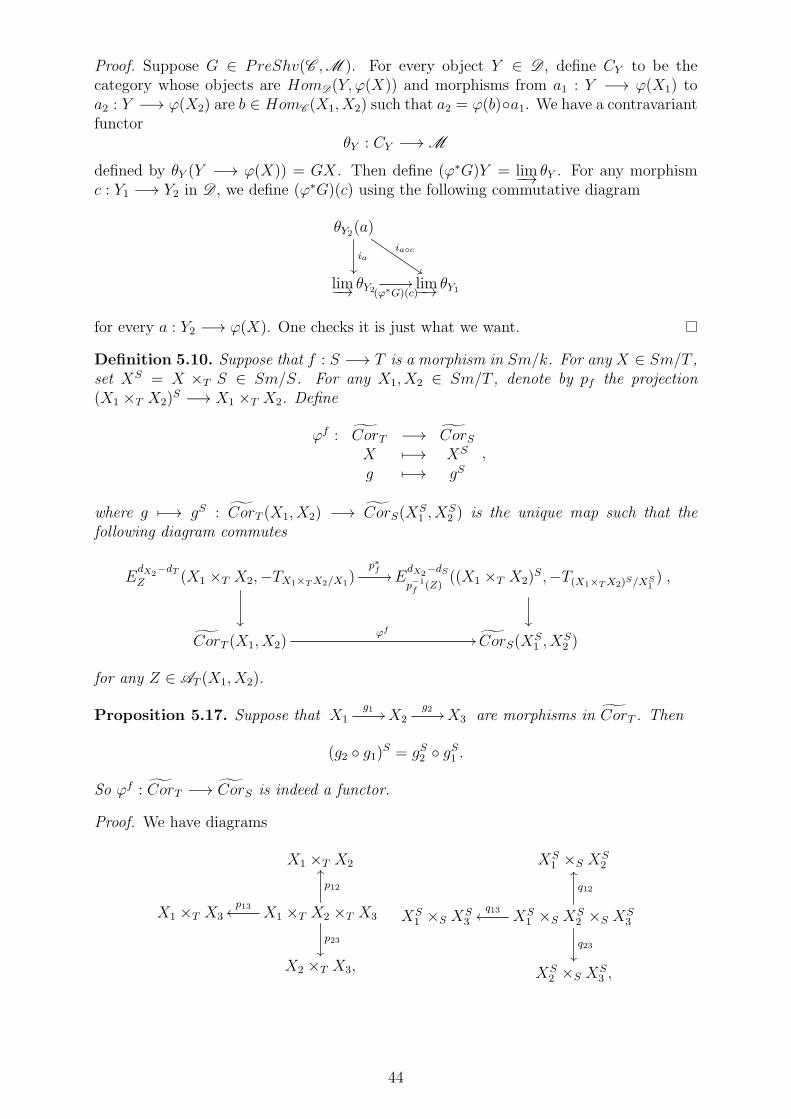
Proof. Suppose G ∈ PreShv(C ,M ). For every object Y ∈ D , define CY to be thecategory whose objects are HomD(Y, ϕ(X)) and morphisms from a1 : Y −→ ϕ(X1) toa2 : Y −→ ϕ(X2) are b ∈ HomC (X1, X2) such that a2 = ϕ(b)a1. We have a contravariantfunctor
θY : CY −→M
defined by θY (Y −→ ϕ(X)) = GX. Then define (ϕ∗G)Y = lim−→ θY . For any morphismc : Y1 −→ Y2 in D , we define (ϕ∗G)(c) using the following commutative diagram
θY2(a)
ia
iac
$$
lim−→ θY2(ϕ∗G)(c)// lim−→ θY1
for every a : Y2 −→ ϕ(X). One checks it is just what we want.
Definition 5.10. Suppose that f : S −→ T is a morphism in Sm/k. For any X ∈ Sm/T ,set XS = X ×T S ∈ Sm/S. For any X1, X2 ∈ Sm/T , denote by pf the projection(X1 ×T X2)
S −→ X1 ×T X2. Define
ϕf : CorT −→ CorSX 7−→ XS
g 7−→ gS,
where g 7−→ gS : CorT (X1, X2) −→ CorS(XS1 , X
S2 ) is the unique map such that the
following diagram commutes
EdX2
−dTZ (X1 ×T X2,−TX1×TX2/X1)
p∗f//
EdX2
−dS
p−1f (Z)
((X1 ×T X2)S,−T(X1×TX2)S/XS
1)
CorT (X1, X2)ϕf
// CorS(XS1 , X
S2 )
,
for any Z ∈ AT (X1, X2).
Proposition 5.17. Suppose that X1g1
// X2g2
// X3 are morphisms in CorT . Then
(g2 g1)S = gS2 g
S1 .
So ϕf : CorT −→ CorS is indeed a functor.
Proof. We have diagrams
X1 ×T X2
X1 ×T X3 X1 ×T X2 ×T X3
p12
OO
p13oo
p23
X2 ×T X3,
XS1 ×S X
S2
XS1 ×S X
S3 XS
1 ×S XS2 ×S X
S3
q12
OO
q13oo
q23
XS2 ×S X
S3 ,
44

and three Cartesian squares
X2 ×S X3
X1 ×T X3 X1 ×T X2 ×T X3p13
oop12
//
p23
OO
X1 ×S X2
XS1 ×S X
S3
r
OO
XS1 ×S X
S2 ×S X
S3
q13oo
t
OO
q23
q12// XS
1 ×S XS2
p
OO
XS2 ×S X
S3 .
q
DD
Suppose that g1 and g2are supported on some admissible subsets. We have
(g2 g1)S
=r∗p13∗(p∗23(g2) · p
∗12(g1))
by definition
=q13∗t∗(p∗23(g2) · p
∗12(g1))
by Axiom 15 for the left square above
=q13∗(q∗12p
∗(g2) · q∗23q
∗(g1))
by Axiom 10 and Axiom 9
=gS2 gS1
by definition.
It’s then easy to verify that γ(idY )S = γ(idY S) for any Y ∈ Sm/T . So ϕf is a functor.
It is straightforward to check that ϕf1f2 = ϕf2 ϕf1 .
Proposition 5.18. Suppose fi ∈ CorT (Xi, Yi) where i = 1, 2. Then
(f1 ×T f2)S = fS1 ×S f
S2 .
Proof. This follows from the commutative diagram
(X1Y1X2Y2)S pf
//
''ww
X1Y1X2Y2
%%yy
(X1Y1)S
pf22(X2Y2)
Spf 22X1Y1 X2Y2.
Proposition 5.19. In the notations above, we have an adjoint pair
f ∗ : Sh(T ) Sh(S) : f∗
where (f∗F )(X) = F ϕf for F ∈ Sh(S).
Proof. Applying Lemma 5.7 to ϕf , we obtain an adjunction PSh(T ) PSh(S).We maythen apply the sheafication functor of Proposition 5.11 to get the desired result.
Obviously, we have (f1 f2)∗ = f ∗
2 f∗1 , (f1 f2)∗ = f1∗ f2∗.
Proposition 5.20. Suppose that f : S −→ T is a morphism in Sm/k.
45
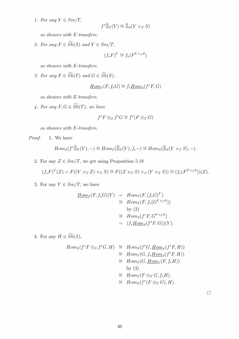
1. For any Y ∈ Sm/T ,
f ∗ZT (Y ) ∼= ZS(Y ×T S)
as sheaves with E-transfers.
2. For any F ∈ Sh(S) and Y ∈ Sm/T ,
(f∗F )Y ∼= f∗(F
Y×TS)
as sheaves with E-transfers.
3. For any F ∈ Sh(T ) and G ∈ Sh(S),
HomT (F, f∗G)∼= f∗HomS(f
∗F,G)
as sheaves with E-transfers.
4. For any F,G ∈ Sh(T ), we have
f ∗F ⊗S f∗G ∼= f ∗(F ⊗T G)
as sheaves with E-transfers.
Proof. 1. We have
HomS(f∗ZT (Y ),−) ∼= HomT (ZT (Y ), f∗−) ∼= HomS(ZS(Y ×T S),−).
2. For any Z ∈ Sm/T , we get using Proposition 5.18
(f∗F )Y (Z) = F ((Y ×T Z)×T S) ∼= F ((Z ×T S)×S (Y ×T S)) ∼= (f∗(F
Y×TS))(Z).
3. For any Y ∈ Sm/T , we have
HomT (F, f∗G)(Y ) = HomT (F, (f∗G)Y )
∼= HomT (F, f∗(GY×TS))
by (2)∼= HomS(f
∗F,GY×TS)
= (f∗HomS(f∗F,G))(Y ).
4. For any H ∈ Sh(S),
HomS(f∗F ⊗S f
∗G,H) ∼= HomS(f∗G,HomS(f
∗F,H))∼= HomT (G, f∗HomS(f
∗F,H))∼= HomT (G,HomT (F, f∗H))
by (3)∼= HomT (F ⊗T G, f∗H)∼= HomS(f
∗(F ⊗T G), H).
46

From now on in this chapter, we suppose that f : S −→ T is a smooth morphism inSm/k. Given such a morphism, we may consider any smooth S-scheme as a smooth T -scheme via f . Moreover, the fact that the diagonal map S → S×T S is a closed immersionimplies that for any smooth S-schemes X1 and X2, the natural morphism
qf : X1 ×S X2 → X1 ×T X2
is a closed immersion. Indeed, this follows from the Cartesian square
X1 ×S X2//
X1 ×T X2
S // S ×T S.
Definition 5.11. For X1, X2 ∈ Sm/S, we define
ϕf : CorS −→ CorTX 7−→ Xg 7−→ gT
,
where g 7−→ gT : CorS(X1, X2) −→ CorT (X1, X2) is the unique map such that the follow-ing diagram commutes
EdX1
−dSZ (X1 ×S X2 − TX1×SX2/X1)
qf∗tf//
EdX1
−dTqf (Z)
(X1 ×T X2,−TX1×TX2/X1)
CorT (X1, X2)ϕf
// CorS(X1, X2)
for any Z ∈ AS(X1, X2). Here, tf is the isomorphism
− TX1×SX2/X1
−→N(X1×SX2)/(X1×TX2) −N(X1×SX2)/(X1×TX2) − TX1×SX2/X1
−→N(X1×SX2)/(X1×TX2) − q∗fTX1×TX2/X1 .
For convenience of notation, we denote TX/Y by Tf for a smooth morphism f : X −→ Yand NX/Y by Nf for a closed immersion f in the following few propositions.
Proposition 5.21. Suppose that X1g1
// X2g2
// X3 are morphisms in CorS. Then,we have
(g2 g1)T = g2T g1T .
So ϕf : CorS −→ CorT is indeed a functor.
Proof. We have Cartesian squares
X1 ×S X2i // X1 ×T X2
X1 ×S X2 ×S X3i′ //
q′12
OO
X1 ×T (X2 ×S X3),
q12
OO
X1 ×T (X2 ×S X3)q
//
r
X1 ×T X2 ×T X3
p23
X2 ×S X3j
// X1 ×T X3,
47

X1 ×S X2 ×S X3//
i′
(X1 ×S X2)×T X3
X1 ×T (X2 ×S X3)q
// X1 ×T X2 ×T X3,
X1 ×S X2 ×S X3
i′
q′13 // X1 ×S X3
k
X1 ×T (X2 ×S X3)p13q
// X1 ×T X3,
and commutative diagrams
X1 ×T X2
X1 ×T (X2 ×S X3)q
//
q12
OO
X1 ×T X2 ×T X3,
p12jj
X1 ×S X2 ×S X3i′ //
q′23 **
X1 ×T (X2 ×S X3)
r
X2 ×S X3.
For g1 and g2 supported on admissible subsets, we have
g2T g1T
=j∗tf (g2) i∗tf (g1)
by definition
=p13∗(p∗23j∗tf (g2) · p
∗12i∗tf (g1))
by definition
=p13∗(q∗r∗tf (g2) · p
∗12i∗tf (g1))
by Axiom 16 for the second square above
=p13∗q∗(r∗tf (g2) · q
∗p∗12i∗tf (g1))
by Axiom 18 for q
=p13∗q∗(r∗tf (g2) · q
∗12i∗tf (g1))
by Axiom 9
=p13∗q∗(r∗tf (g2) · i
′∗q
′∗12tf (g1))
by Axiom 16 for the first square above
=p13∗q∗i′∗(i
′∗r∗tf (g2) · q′∗12tf (g1))
by Axiom 18 for i′
=p13∗q∗i′∗((q
′∗23tf (g2) · q
′∗12tf (g1), i
′∗Nq − i′∗q∗p∗13TX1×TX3/X1 +Ni′ − i
′∗q∗Tp13))
by Axiom 9
=(p13 q)∗i′∗((q
′∗23tf (g2) · q
′∗12tf (g1),−i
′∗q∗p∗13TX1×TX3/X1 +Ni′ − i′∗Tp13q))
by Axiom 19, (1) and functoriality of push-forwards with respect to twists
=k∗q′13∗((q
′∗23tf (g2) · q
′∗12tf (g1),−q
′∗13k
∗TX1×TX3/X1 + q′∗13Nk − Tq′13))
by Axiom 19, (3) for the last square above.
Now, we have to treat the twists. We say that a morphism f : A + B −→ C +D ina Picard category contains a switch if there are morphisms g : A −→ D and h : B −→ Csuch that f = c(D,C) (g + h). Conversely, we say that it doesn’t contain a switch if
48
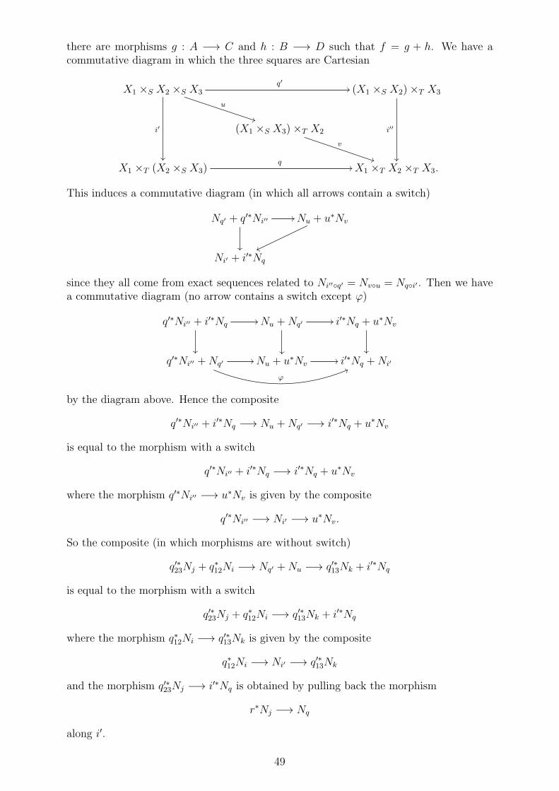
there are morphisms g : A −→ C and h : B −→ D such that f = g + h. We have acommutative diagram in which the three squares are Cartesian
X1 ×S X2 ×S X3q′
//
u
**
i′
(X1 ×S X2)×T X3
i′′
(X1 ×S X3)×T X2
v
**
X1 ×T (X2 ×S X3)q
// X1 ×T X2 ×T X3.
This induces a commutative diagram (in which all arrows contain a switch)
Nq′ + q′∗Ni′′//
Nu + u∗Nv
ww
Ni′ + i′∗Nq
since they all come from exact sequences related to Ni′′q′ = Nvu = Nqi′ . Then we havea commutative diagram (no arrow contains a switch except ϕ)
q′∗Ni′′ + i′∗Nq//
Nu +Nq′//
i′∗Nq + u∗Nv
q′∗Ni′′ +Nq′//
ϕ
66Nu + u∗Nv
// i′∗Nq +Ni′
by the diagram above. Hence the composite
q′∗Ni′′ + i′∗Nq −→ Nu +Nq′ −→ i′∗Nq + u∗Nv
is equal to the morphism with a switch
q′∗Ni′′ + i′∗Nq −→ i′∗Nq + u∗Nv
where the morphism q′∗Ni′′ −→ u∗Nv is given by the composite
q′∗Ni′′ −→ Ni′ −→ u∗Nv.
So the composite (in which morphisms are without switch)
q′∗23Nj + q∗12Ni −→ Nq′ +Nu −→ q′∗13Nk + i′∗Nq
is equal to the morphism with a switch
q′∗23Nj + q∗12Ni −→ q′∗13Nk + i′∗Nq
where the morphism q∗12Ni −→ q′∗13Nk is given by the composite
q∗12Ni −→ Ni′ −→ q′∗13Nk
and the morphism q′∗23Nj −→ i′∗Nq is obtained by pulling back the morphism
r∗Nj −→ Nq
along i′.
49
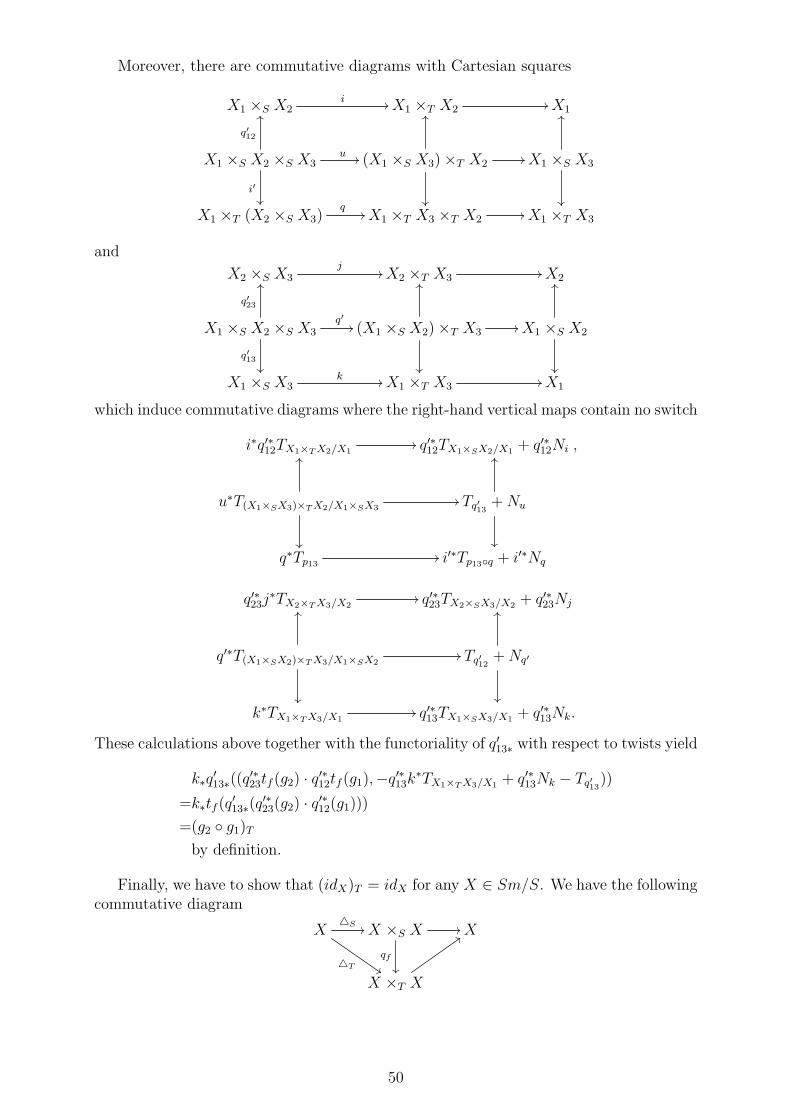
Moreover, there are commutative diagrams with Cartesian squares
X1 ×S X2i // X1 ×T X2
// X1
X1 ×S X2 ×S X3
q′12
OO
u //
i′
(X1 ×S X3)×T X2//
OO
X1 ×S X3
OO
X1 ×T (X2 ×S X3)q
// X1 ×T X3 ×T X2// X1 ×T X3
and
X2 ×S X3j
// X2 ×T X3// X2
X1 ×S X2 ×S X3q′
//
q′23
OO
q′13
(X1 ×S X2)×T X3
OO
// X1 ×S X2
OO
X1 ×S X3k // X1 ×T X3
// X1
which induce commutative diagrams where the right-hand vertical maps contain no switch
i∗q′∗12TX1×TX2/X1// q′∗12TX1×SX2/X1 + q′∗12Ni
u∗T(X1×SX3)×TX2/X1×SX3//
OO
Tq′13 +Nu
OO
q∗Tp13 // i′∗Tp13q + i′∗Nq
,
q′∗23j∗TX2×TX3/X2
// q′∗23TX2×SX3/X2 + q′∗23Nj
q′∗T(X1×SX2)×TX3/X1×SX2//
OO
Tq′12 +Nq′
OO
k∗TX1×TX3/X1// q′∗13TX1×SX3/X1 + q′∗13Nk.
These calculations above together with the functoriality of q′13∗ with respect to twists yield
k∗q′13∗((q
′∗23tf (g2) · q
′∗12tf (g1),−q
′∗13k
∗TX1×TX3/X1 + q′∗13Nk − Tq′13))
=k∗tf (q′13∗(q
′∗23(g2) · q
′∗12(g1)))
=(g2 g1)T
by definition.
Finally, we have to show that (idX)T = idX for any X ∈ Sm/S. We have the followingcommutative diagram
X
T $$
S // X ×S X //
qf
X
X ×T X
::
50
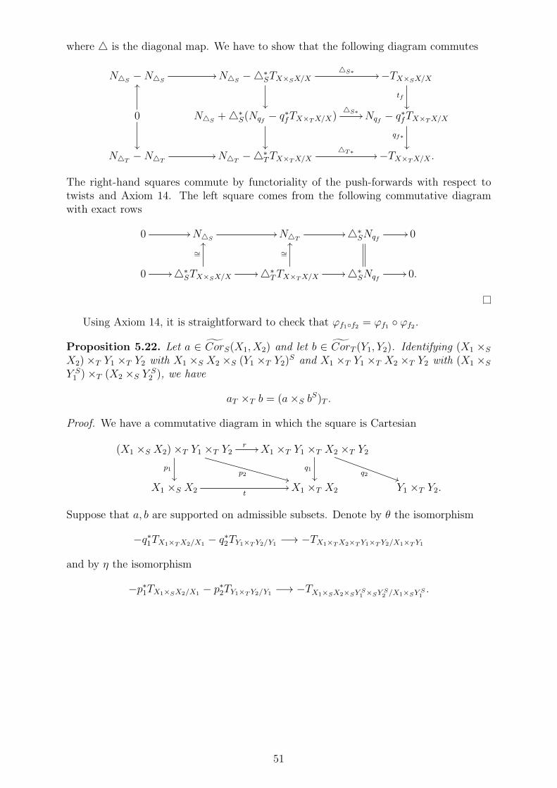
where is the diagonal map. We have to show that the following diagram commutes
NS−NS
// NS−∗
STX×SX/X
S∗ // −TX×SX/X
tf
0
OO
NS+∗
S(Nqf − q∗fTX×TX/X)
S∗ //
Nqf − q∗fTX×TX/X
qf∗
NT−NT
// NT−∗
TTX×TX/XT∗ // −TX×TX/X .
The right-hand squares commute by functoriality of the push-forwards with respect totwists and Axiom 14. The left square comes from the following commutative diagramwith exact rows
0 // NS// NT
//∗SNqf
// 0
0 //∗STX×SX/X
∼=
OO
//∗TTX×TX/X
∼=
OO
//∗SNqf
// 0.
Using Axiom 14, it is straightforward to check that ϕf1f2 = ϕf1 ϕf2 .
Proposition 5.22. Let a ∈ CorS(X1, X2) and let b ∈ CorT (Y1, Y2). Identifying (X1 ×SX2)×T Y1 ×T Y2 with X1 ×S X2 ×S (Y1 ×T Y2)
S and X1 ×T Y1 ×T X2 ×T Y2 with (X1 ×SY S1 )×T (X2 ×S Y
S2 ), we have
aT ×T b = (a×S bS)T .
Proof. We have a commutative diagram in which the square is Cartesian
(X1 ×S X2)×T Y1 ×T Y2r //
p1
p2
++
X1 ×T Y1 ×T X2 ×T Y2
q1
q2
))
X1 ×S X2 t// X1 ×T X2 Y1 ×T Y2.
Suppose that a, b are supported on admissible subsets. Denote by θ the isomorphism
−q∗1TX1×TX2/X1 − q∗2TY1×TY2/Y1 −→ −TX1×TX2×TY1×TY2/X1×TY1
and by η the isomorphism
−p∗1TX1×SX2/X1 − p∗2TY1×TY2/Y1 −→ −TX1×SX2×SY
S1 ×SY
S2 /X1×SY
S1.
51

Then
aT ×T b
=θ(q∗1t∗(tf (a)) · q∗2b)
by definition
=θ(r∗p∗1(tf (a)) · q
∗2b)
by Axiom 16 for the square in the diagram
=θ(r∗(p∗1(tf (a)) · p
∗2b))
by Proposition 18 for r and Axiom 10
=r∗r∗(θ)((p∗1(tf (a)) · p
∗2b, p
∗1Nt − p
∗1t
∗TX1×TX2/X1 − p∗2TY1×TY2/Y1))
by functoriality of push-forwards with respect to twists
=r∗(tf (η(p∗1(a) · p
∗2b)))
=(a×S bS)T
by definition.
Here the fifth equality comes from the following commutative diagram with exact rowsand columns
0
0
p∗2TY1×TY2/Y1
p∗2TY1×TY2/Y1
0 // r∗TX1Y1X2Y2/X1Y1//
TX1X2Y S1 Y
S2 /X1Y S
1
// Nr//
∼=
0
0 // r∗q∗1TX1×TX2/X1//
p∗1TX1×SX2/X1//
p∗1Nt// 0
0 0
and Theorem 3.1, (1).
Applying the same proof as in Proposition 5.19 to ϕf , we get the following result.
Proposition 5.23. There is an adjoint pair
f# : Sh(S) Sh(T ) : (f#)′,
where (f#)′F = F ϕf for F ∈ Sh(T ).
The next lemma is important when identifying (f#)′. See also [MVW06, Exercise
1.12].
Lemma 5.8. For any U ∈ Sm/S, X ∈ Sm/T , we have an adjoint pair:
CorS(U,XS) = CorT (U,X).
Proof. For any U ∈ Sm/S, X ∈ Sm/T , we have an isomorphism
θU,X : U ×S XS −→ U ×T X.
52

We can then define
λU,X : CorS(U,XS) −→ CorT (U,X)
W 7−→ θU,X∗(W ),
which is obviously an isomorphism.Let now U ∈ Sm/S, X1, X2 ∈ Sm/T , V ∈ CorT (X1, X2) and W ∈ CorS(U,X
S1 ). We
want to show thatλU,X2(V
S W ) = V λU,X1(W ).
We have a commutative diagram
X1 ×T X2 U ×T X1
XS1 ×S X
S2
p
OO
U ×S XS1
θU,X1
∼=
88
U ×S (XS1 ×S X
S2 )
p23
OO
p13//
p1266
q23
@@q12
00
q13
66U ×S X
S2
θU,X2
∼=// U ×T X2,
where we have identified U ×S (XS1 ×S X
S2 ) with U ×T X1 ×T X2 for convenience.
Suppose that V and W are supported on admissible subsets. We then have
λU,X2(VS W ) = θU,X2∗p13∗(p
∗23p
∗V · p∗12W )
by definition
= q13∗(q∗23V · p
∗12W )
by Axiom 12
= q13∗(q∗23V · q
∗12θU,X1∗W )
by Axiom 20 and Axiom 9
= V λU,X1(W )
by definition.
Suppose next that U1, U2 ∈ Sm/S,X ∈ Sm/T , V ∈ CorS(U1, U2) andW ∈ CorS(U2, XS).
We want to show thatλU1,X(W V ) = λU2,X(W ) VT .
We have a commutative diagram
U1 ×T U2 U1 ×T (U2 ×S XS)doo b //
q23
((
q13++
U2 ×S XSθU2,X // U2 ×T X
U1 ×S U2
qf
OO
U1 ×S (U2 ×S XS)
p12oo
p13//
p23
66
a
OO
U1 ×S XSθU1,X
// U1 ×T X
,
where we have identified U1×T (U2×SXS) with U1×T U2×TX. If V andW are supported
on admissible subsets and θ is the isomorphism
−TU1×SU2×SXS/U1×TX −→ Na − a∗TU1×T (U2×SXS)/U1×TX ,
53
we have
λU1,X(W V )
=θU1,X∗p13∗((p∗23W · p
∗12V,−TU1×SU2×SXS/U2×SXS − p∗12TU1×SU2/U1))
by definition
=q13∗a∗((a∗q∗23θU2,X∗W · θ(p
∗12V ),−a∗q∗23TU2×TX/U2 +Na − a
∗TU1×T (U2×SXS)/U1×TX))
by Axiom 20 and Axiom 19, (1)
=q13∗((q∗23θU2,X∗W · a∗θ(p
∗12V ),−q∗23TU2×TX/U2 − TU1×T (U2×SXS)/U1×TX))
by Axiom 18 for a
=q13∗((q∗23θU2,X∗W · d
∗qf∗ϕf (V ),−q∗23TU2×TX/U2 − d∗TU1×TU2/U1))
by Axiom 16 for the leftmost square in the diagram above
=λU2,X(W ) VT
by definition.
Proposition 5.24. Let f : S → T be a smooth morphism. Then
(f#)′ = f ∗.
Proof. For any Y ∈ Sm/S, γ(idY ) ∈ CorT (Y, Y ) = CorS(Y, YS) is the initial element of
CY in Lemma 5.7 by application of the above lemma to ϕf (see Definition 5.10). So for
any F ∈ PSh(T ), we have (f ∗F )(Y ) = FY = ((f#)′F )(Y ). This gives an isomorphism
between f ∗(F ) and (f#)′(F ) for any presheaf with E-transfers F by the lemma above. So
it also gives an isomorphism after sheafication.
Proposition 5.25. Let f : S −→ T be a smooth morphism. Then:
1. For any X ∈ Sm/S, we have
f#ZS(X) ∼= ZT (X).
as sheaves with E-transfers.
2. For any F ∈ Sh(T ) and Y ∈ Sm/T
f ∗(F Y ) ∼= (f ∗F )Y×TS
as sheaves with E-transfers.
3. For any F ∈ Sh(S) and G ∈ Sh(T )
HomT (f#F,H) ∼= f∗HomS(F, f∗H)
as sheaves with E-transfers.
4. For any F ∈ Sh(S) and G ∈ Sh(T )
f#(F ⊗S f∗G) ∼= f#F ⊗T G
as sheaves with E-transfers.
Proof. 1. The result follows from the fact that any F ∈ Sh(T ) we have
HomT (f#ZS(X), F ) ∼= HomS(ZS(X), f ∗F ) ∼= (f ∗F )(X) ∼= F (X)
by the previous proposition.
54

2. For any X ∈ Sm/S, we get
(f ∗(HY ))(X) = H(Y ×T X).
and(f ∗H)Y×TS(X) = H((Y ×T S)×S X)
by the above proposition. Then, we can use Proposition 5.22 to conclude.
3. For any Y ∈ Sm/T , we have
HomT (f#F,H)(Y ) = HomT (f#F,HY )
∼= HomS(F, f∗(HY ))
∼= HomS(F, (f∗H)Y×TS)
by (2)
= HomS(F, f∗H)(Y ×T S)
= (f∗HomS(F, f∗H))(Y ).
4. For any H ∈ Sh(T ), the following computation applies:
HomT (f#(F ⊗S f∗G), H) ∼= HomS(F ⊗S f
∗G, f ∗H)∼= HomS(f
∗G,HomS(F, f∗H))
∼= HomT (G, f∗HomS(F, f∗H))
∼= HomT (G,HomT (f#F,H))
by (3)∼= HomT (f#F ⊗T G,H).
55

Chapter 6
Motivic categories
In this chapter, we construct the categories of effective (resp. stabilized) motives asa localization of the bounded above complexes ([MVW06]) of sheaves with E-transfers(resp. symmetric spectra). We then compare our construction with the constructions in[CD09], [CD13] and [DF17], where they use unbounded complexes.
6.1 Complexes of Sheaves with E-Transfers
6.1.1 Derived Categories
Denote by D−(S) (resp. K−(S)) the derived (resp. homotopy) category of bounded above
complexes of objects in Sh(S). Our first aim is to define ⊗S and f# and f ∗ (Chapter 5)at the level of these categories. The method is inherited from [SV00, Corollary 2.2] and[MVW06, Lemma 8.15].
Definition 6.1. We call a presheaf with E-transfers free if it’s a direct sum of presheavesof the form cS(X). We call a presheaf with E-transfers projective if it’s a direct summandof a free presheaf with E-transfers. A sheaf with E-transfers is called free (resp. projective)if it’s a sheafication of a free (resp. projective) presheaf with E-transfers. A boundedabove complex of sheaves with E-transfers is called free (projective) if all its terms arefree (projective).
Remark 6.1. Note that a projective presheaf with E-transfers is a projective object inthe category of presheaves with E-transfers. On the other hand, this is not true anymorefor projective sheaves with E-transfers.
Definition 6.2. A projective resolution of a bounded above complex of sheaves K is aprojective complex (of sheaves) with a quasi-isomorphism P −→ K.
In the definition above, if K is already projective we may take P = K.
Now let S, T ∈ Sm/k and Y be a scheme with morphisms S Yf
oog
// T where gis smooth. In this section, we consider the functors
ϕ : CorS −→ CorTX 7−→ (XY )T ∼= X ×S Y
andψ : SmS −→ SmT
X 7−→ X ×S Y
56
determined by the triple (Y, S, T ). We have a commutative diagram
Sm/Sψ
//
γ
Sm/T
γ
CorSϕ
// CorT .
Recall from Lemma 5.7 the definitions of ϕ∗ and ϕ∗.
Lemma 6.1. For any X ∈ Sm/S, we have
ϕ∗(cS(X)) ∼= cT (ψ(X))
as presheaves with E-transfers.
Proof. For any F ∈ PSh(T ),
HomT (ϕ∗(cS(X)), F ) ∼= HomS(cS(X), ϕ∗F ) ∼= F (ψ(X)).
Lemma 6.2. The functor ϕ∗ maps sheaves with E-transfers to sheaves with E-transfers.
Proof. It suffices to show that for any finite Nisnevich covering Ui of X ∈ Sm/S, thefollowing sequence is exact
0 −→ G(X) −→ ⊕iG(Ui) −→ ⊕i,jG(Ui ×X Uj)
where G = ϕ∗F for some F ∈ Sh(T ). This follows easily.
The following lemma can be proved using a method similar to the one we used in theproof of Proposition 5.15.
Lemma 6.3. Let f : F −→ G be morphism in PSh(S) such that a(f) is an isomorphism,then a(ϕ∗(f)) is also an isomorphism.
Before stating the next result, recall that the category of presheaves with E-transfershas enough projective objects (see for instance Remark 6.1). In particular, it is possibleto derive any left-exact functor (say, to the category of abelian groups).
Proposition 6.1. For any F ∈ PSh(S),
a((Liϕ∗)a(F )) ∼= a((Liϕ
∗)F )
as sheaves with E-transfers for any i ≥ 0, where Liϕ∗ means the ith left derived functor
of ϕ∗.
Proof. We show first that for any presheaf with E-transfers F with a(F ) = 0 we have
a(Liϕ∗(F )) = 0
for any i ≥ 0. Suppose that the above statement is proved. For any presheaf withE-transfers F , we can then consider the natural morphism
θ : F −→ a(F ).
57
We havea(coker(θ)) = a(ker(θ)) = 0.
Hence for any i ≥ 0, we have
a(Liϕ∗a(F )) ∼= a(Liϕ
∗Im(θ)) ∼= a(Liϕ∗F )
by using long exact sequences. Hence the statement follows.Now we prove the first claim by induction on i. The claim is true for i = 0 and we
then suppose that it’s true for i < n. For any F ∈ PSh(S), we have a surjection
⊕x∈F (X)cS(X) −→ F
defined by each section of F on each X ∈ Sm/S. Since a(F ) = 0, there exists for anyX ∈ Sm/S and any x ∈ F (X) a finite Nisnevich covering Ux −→ X of X such thatx|Ua = 0. Then, the composite
⊕x∈F (X)cS(Ux) −→ ⊕x∈F (X)cS(X) −→ F
is trivial and we obtain a surjection
⊕x∈F (X)H0(C(Ux/X)) −→ F
with kernel K. Proposition 5.10 implies that
a(Hp(C(U/X))) = 0
for any Nisnevich covering U −→ X and any p ∈ Z and consequently a(K) = 0 as well.We have a hypercohomology spectral sequence
(Lpϕ∗)Hq(C(U/X)) =⇒ (Lp+qϕ
∗)C(U/X).
Hencea((Lnϕ
∗)C(U/X)) ∼= a((Lnϕ∗)H0(C(U/X)))
by induction hypothesis. But
a((Lnϕ∗)C(U/X)) ∼= a(Hn(ϕ
∗C(U/X)))
by definition of hypercohomology and the latter vanishes since we have
ϕ∗C(U/X) = C(ψU/ψX)
by the previous lemmas. So
a((Lnϕ∗)H0(C(U/X))) = 0
anda(Lnϕ
∗F ) ∼= a(Ln−1ϕ∗K) = 0
by the long exact sequence and the induction hypothesis.
Proposition 6.2. The functor ϕ∗ takes acyclic projective complexes to acyclic projectivecomplexes.
58

Proof. For any projective F ∈ Sh(S), F = a(G) for some projective G ∈ PSh(S) bydefinition. So
a((Liϕ∗)F ) ∼= a((Liϕ
∗)G) = 0
for any i > 0 by the proposition above. Let
0 −→ K −→ F −→ P −→ 0
be a short exact sequence of sheaves with E-transfers with a((Liϕ∗)P ) = 0 for any i > 0.
Then the sequence is still exact after applying ϕ∗ by the long exact sequence. Then thestatement follows easily.
Proposition 6.3. We have an exact functor
Lϕ∗ : D−(S) −→ D−(T )
which maps any K ∈ D−(S) to ϕ∗P , where P is a projective resolution K.
Proof. By the proposition above, the class of projective complexes is adapted (see [GM03,III.6.3]) to the functor ϕ∗. We may now apply [GM03, III.6.6].
In the sequel, we’ll write ϕ∗ in place of Lϕ∗ for convenience. We now apply the generalresults above to ⊗S, f# and f ∗.
Proposition 6.4. 1. The category D−(S) is endowed with a tensor product defined by
⊗S : D−(S) × D−(S) −→ D−(S)(K , L) 7−→ P ⊗S Q
,
where P,Q are projective resolutions of K,L respectively, and P ⊗S Q is the totalcomplex of the bicomplex Pi ⊗S Qj. Moreover, for any K ∈ D−(S), the functorK ⊗S − is exact.
2. Suppose that f : S −→ T is a smooth morphism in Sm/k. Then, there is an exactfunctor
f# : D−(S)→ D−(T )
defined on objects by K 7→ f#P , where P is a projective resolution of K.
3. Suppose that f : S −→ T is a morphism in Sm/k. There is an exact functor
f ∗ : D−(T )→ D−(S)
defined on objects by K 7→ f ∗P , where P is a projective resolution of K.
Proof. 1. Let Y ∈ Sm/S. In the definition of ϕ, we take (Y, S, T ) := (Y, S, S) and
then ϕ∗F ∼= F ⊗S ZS(Y ) for any F ∈ Sh(S) by Proposition 5.14.
Given an acyclic projective complex P and a projective sheaf F , the complex ofsheaves F ⊗S P is also acyclic by Proposition 6.2 and by definition of projectiveness.It follows that for any projective complex K the complex P ⊗S K is also acyclicby the spectral sequence of the bicomplex Pi ⊗S Kj. Then for any projectivecomplexes P,Q,R and quasi-isomorphism a : P −→ Q, the morphism a⊗SR is stilla quasi-isomorphism since we have
Cone(a⊗S R) ∼= Cone(a)⊗S R
and the latter one acyclic. The statement follows easily.
59

2. In the definition of ϕ, we take (Y, S, T ) := (S, S, T ) and apply Proposition 6.3.
3. In the definition of ϕ, we take (Y, S, T ) := (T, S, T ) and apply Proposition 6.3.
Proposition 6.5. Let f : S −→ T be a smooth morphism in Sm/k. We then have anadjoint pair
f# : D−(S) D−(T ) : f ∗.
Proof. By Proposition 5.23, it is easy to see that there is an adjunction
f# : K−(S) K−(T ) : f ∗.
Since f ∗ : Sh(T ) −→ Sh(S) has both a left adjoint and a right adjoint, it’s an exactfunctor and Lf ∗ ∼= f ∗ in this case. Suppose that K ∈ D−(S), L ∈ D−(T ) and thatp : P −→ K is a projective resolution of K. Note then that f#K = f#P by definition.
We now construct a morphism
θ : HomD−(S)(f#K,L) −→ HomD−(T )(K, f∗L)
as follows. Suppose that s ∈ HomD−(S)(f#K,L) is written as a right roof (see [GM03,III.2.9])
R
f#P
a
==
L.b
__
By adjunction, a induces a morphism a′ : P −→ f ∗R. Then we define θ(s) to thecomposite of the right roof
f ∗R
Pa′
==
f ∗Lf∗b
bb
with p−1. This morphism is well-defined since f ∗ is exact.Next, we construct a morphism
ξ : HomD−(T )(K, f∗L) −→ HomD−(S)(f#K,L)
as follows. Suppose that t ∈ HomD−(T )(K, f∗L) and that t p is written as a left roof
(see [GM03, III.2.8])R
a
b
!!
P f ∗L
where R is also projective. By adjunction, b induces a morphism b′ : f#R −→ L and wedefine ξ(t) to be the left roof
f#Rf#a
||
b′
!!
f#P L.
This morphism is well-defined by Proposition 6.2 applied to f#. To conclude, one checksthat θ and ξ are inverse to each other by direct computation.
60

In [CD09, Theorem 1.7], they put a model structure M on the category of unboundedcomplexes of sheaves with E-transfers over S. This is a cofibrantly generated modelstructure where the cofibrations are the I-cofibrations ([Hov07, Definition 2.1.7]) where I
consists of the morphisms Sn+1ZS(X) −→ DnZS(X) for any X ∈ Sm/S ([CD09, 1.9] fornotations) and weak equivalences are quasi-morphisms of complexes.
Proposition 6.6. Bounded above projective complexes are cofibrant objects in M.
Proof. Suppose that P is a bounded above projective complex and that we have an I-injective ([Hov07, Definition 2.1.7]) morphism f : A −→ B between unbounded complexeswith a morphism g : P −→ B. We have to show that g = f h for some h : P −→ A.
We construct h by induction. Suppose that for any m ≥ n we have constructed amorphism hm : Pm −→ Am such that gm = fm hm and dA hm = hm dP . AsP is bounded above, this is certainly the case for n large enough. We now constructhn−1 : P n−1 −→ An−1 satisfying the same property, that is, making the following diagramcommute
An−1 dA //
fn−1
An
fn
P n−1
hn−1
dd
gn−1zz
dP // P n
hnaa
gn
Bn−1 dB // Bn.
By definition, we have a split surjection F −→ P n−1 where F is a free sheaf with E-transfers. So, we may assume that P n−1 is free of the form ⊕iZS(Xi) where Xi ∈ Sm/S.For every i, we have two morphisms:
ui : ZS(Xi) −→ P n−1 −→ Bn−1 −→ Bn
andvi : ZS(Xi) −→ P n−1 −→ P n −→ An
which give a commutative square with a lifting since f is I-injective:
SnZS(Xi)vi //
A
f
Dn−1ZS(Xi)ui //
wi
::
B.
One checks directly that ⊕iwi : Pn−1 −→ An−1 is the required morphism.
The model structure M is stable and left proper so it induces a triangulated structureT′ on D(S) ([Ayo07, Theoreme 4.1.49]). The classical triangulated structure of D(S) orD−(S) is denoted by T.
Proposition 6.7. The natural functor
i : (D−(S),T) −→ (D(S),T′)
is fully faithful exact.
Proof. Any distinguished triangle T in (D−(S),T) is isomorphic in D−(S) to a distin-guished triangle in T of the form
Af
// B // Cone(f) // A[1] ,
61

where all arrows come from explicit morphisms between chain complexes ([GM03, III.3.3and III.3.4]). By [Hir03, Proposition 8.1.23], there exists a commutative diagram
A′ g//
a
B′
b
Af
// B
such that (A′, a) (resp. (B′, b)) is a fibrant cofibrant approximation of A (resp. B) andg is a cofibration in M. So the triangle T is isomorphic in D(S) to the distinguishedtriangle
A′ g// B′ // Cone(g) // A′[1]
in T. By [CD09, Lemma 1.10] and [Ayo07, Theoreme 4.1.38], the shift functors −[n] and−[n]′ in T and T′, respectively, coincide on cofibrant objects in M. So we have a naturalisomorphism η : −[n] −→ −[n]′ where ηK = idK[n] if K is cofibrant in M. It follows thatthe triangle above is distinguished in T′ by [Ayo07, Definition 4.1.45]. So the functor i isexact and it’s clearly fully faithful.
Observe now that we can define ⊗S, f∗ and f# on D(S) by [CD09, Theorem 1.18 and
Proposition 2.3].
Proposition 6.8. 1. We have a commutative diagram (up to a natural isomorphism)
D−(S)×D−(S)⊗S //
D−(S)
D(S)×D(S)⊗S // D(S).
2. Suppose that f : S −→ T is a morphism in Sm/k. We have a commutative diagram(up to a natural isomorphism)
D−(T )f∗
//
D−(S)
D(T )f∗
// D(S)
3. Suppose that f : S −→ T is a smooth morphism in Sm/k. We have a commutativediagram (up to a natural isomorphism)
D−(S)f#
//
D−(T )
D(S)f#
// D(T )
Proof. This follows by direct computation using Proposition 6.6.
6.1.2 Effective Motives
The following definition comes from [MVW06, Definition 9.2].
Definition 6.3. Define EA to be the smallest thick subcategory of D−(S) such that
62

1. Cone(ZS(X ×k A1) −→ ZS(X)) ∈ EA.
2. EA is closed under arbitrary direct sums if it exists in D−(S).
Set WA to be the class of morphisms in D−(S) whose cone is in EA. Define
DMeff,−
(S) = D−(S)[W−1A ]
to be the category of effective motives over S. The morphisms in D−(S) becoming iso-morphisms after localization by WA are called A1-weak equivalences.
Before proceeding further, we give an example of an A1-weak equivalence. Recall thata morphism p : E −→ X in Sm/S is an An-bundle if there is an open covering Ui of Xsuch that p−1(Ui) ∼= Ui ×k A
n for any i.
Proposition 6.9. Let p : E −→ X in Sm/S be an An-bundle. Then, ZS(p) : ZS(E) −→
ZS(X) is an A1-weak equivalence.
Proof. For any X ∈ Sm/S, the projection ZS(X ×k An) −→ ZS(X) is an A1-weakequivalence by definition. Suppose that we have two open sets U1 and U2 of X suchthat the statement is true over U1, U2 and U1 ∩ U2 and set Ei = p−1(Ui). We have acommutative diagram with exact rows
0 // ZS(E1 ∩ E2) //
ZS(E1)⊕ ZS(E2) //
ZS(p−1(E1 ∪ E2)) //
0
0 // ZS(U1 ∩ U2) // ZS(U1)⊕ ZS(U2) // ZS(U1 ∪ U2) // 0
by Proposition 5.12. So the statement is also true over U1 ∪ U2. To conclude, we pick afinite open covering Ui of X such that p−1(Ui) ∼= Ui ×k A
n for every i and proceed byinduction on the number of open sets.
Definition 6.4. ([MVW06, Definition 9.17]) A complex K ∈ D−(S) is called A1-local iffor every A1-equivalence f : A −→ B, the induced map
HomD−(S)(B,K) −→ HomD−(S)(A,K)
is an isomorphism.
Before stating the next result, recall that one can associate to any complex of sheavesK its Suslin complex C∗K ([MVW06, Definition 2.14]).
Proposition 6.10. Let K ∈ D−(S).
1. The natural map K −→ C∗K is an A1-weak equivalence.
2. If S = pt, the complex C∗K is A1-local.
3. If S = pt, the functor C∗ induces an endofunctor of D−(pt).
Proof. 1. The proof of [MVW06, Lemma 9.15] goes through in our setting.
2. Use Remark 5.1 and mimic the proof of [DF17, Theorem 3.2.9 and Corollary 3.2.11].
63

3. It’s easy to check that C∗ induces an endofunctor of K−(pt). If f : K −→ Lis a quasi-isomorphism, then Cone(f) is acyclic. By (1), the natural morphismCone(f) −→ C∗Cone(f) is an A1-equivalence. Hence it’s an quasi-isomorphism by(2) and [MVW06, Lemma 9.21]. So C∗Cone(f) = Cone(C∗f) is acyclic and C∗f isa quasi-isomorphism.
We now pass to the definition of motivic cohomology.
Definition 6.5. ([MVW06, Definition 14.17]) Let X ∈ Sm/k and let p, q ∈ Z, q ≥ 0.The groups
Hp,qE (X,Z) = Hom
DMeff,−
(pt)(Zpt(X), Zpt(q)[p])
are called E-motivic cohomology groups of X.
Proposition 6.11. The functor ϕ of Proposition 6.3 induces an exact functor
ϕ∗ : DMeff,−
(S) −→ DMeff,−
(T )
which is determined by the following commutative diagram
D−(S)ϕ∗
//
D−(T )
DMeff,−
(S)ϕ∗
// DMeff,−
(T ).
Proof. Let E be the full subcategory of D−(S) which consists of those complexes K ∈D−(S) who satisfy ϕ∗K ∈ EA. It’s a thick subcategory of D−(S). For any X ∈ Sm/S,ϕ∗ maps
ZS(X ×k A1) −→ ZS(X)
toZT ((ψX)×k A
1) −→ ZT (ψX).
Therefore EA ⊆ E by definition of EA and exactness of ϕ∗. It follows that ϕ∗ preservesobjects in EA. Hence ϕ∗ preserves A1-weak equivalences by exactness of ϕ∗. Then thestatement follows from [Kra10, Proposition 4.6.2].
Proposition 6.12. 1. There is a tensor product
⊗S : DMeff,−
(S)× DMeff,−
(S) −→ DMeff,−
(S)
which is determined by the following commutative diagram
D−(S)×D−(S)⊗S //
D−(S)
DMeff,−
(S)× DMeff,−
(S)⊗S // DM
eff,−(S).
Furthermore, for any K ∈ DMeff,−
(S), the functor K ⊗S − is exact.
2. Suppose that f : S −→ T is a smooth morphism in Sm/k. There is an exact functor
f# : DMeff,−
(S) −→ DMeff,−
(T )
64
which is determined by the following commutative diagram
D−(S)f#
//
D−(T )
DMeff,−
(S)f#
// DMeff,−
(T ).
3. Suppose that f : S −→ T is a morphism in Sm/k. There is an exact functor
f ∗ : DMeff,−
(T ) −→ DMeff,−
(S)
which is determined by the following commutative diagram
D−(T )f∗
//
D−(S)
DMeff,−
(T )f∗
// DMeff,−
(S).
Proof. 1. Suppose that Y ∈ Sm/S. In the definition of ϕ, we take (Y, S, T ) :=
(Y, S, S). Then ϕ∗F ∼= F ⊗S ZS(Y ) for any F ∈ Sh(S) by Proposition 5.14. Now,
given an A1-weak equivalence a, ZS(Y )⊗Sa is also an A1-weak equivalence by Propo-sition 6.11 (applied to ϕ). We may now apply the method used in the third para-graph of [MVW06, Lemma 9.5] to show that the functorK⊗S− : D−(S) −→ D−(S)preserves A1-weak equivalences for any K ∈ D−(S). Finally we apply [Kra10,Proposition 4.6.2] to the functor K ⊗S −.
2. In the definition of ϕ, we take (Y, S, T ) := (S, S, T ) and apply Proposition 6.11.
3. In the definition of ϕ, we take (Y, S, T ) := (T, S, T ) and apply Proposition 6.11.
Proposition 6.13. Let f : S −→ T be a smooth morphism in Sm/k. We have an adjointpair
f# : DMeff,−
(S) DMeff,−
(T ) : f ∗.
Proof. The same method as in Proposition 6.5 applies since ϕ∗ preserves EA by Proposition6.11.
Proposition 6.14. Let f : S −→ T be a morphism in Sm/k.
1. For any K,L ∈ DMeff,−
(T ), we have
f ∗(K ⊗S L) ∼= (f ∗K)⊗S (f∗L).
2. If f is smooth, then for any K ∈ DMeff,−
(S) and L ∈ DMeff,−
(T ), we have
f#(K ⊗S f∗L) ∼= (f#K)⊗S L.
Proof. This follows immediately from Proposition 5.20 and Proposition 5.25.
In [CD09, Proposition 3.5] and [DF17, Definition 3.2.1], the category DMeff
(S) isdefined as the the Verdier localization of D(S) with respect to the homotopy invariance
conditions. Now, this localization induces a triangulated structure on DMeff
(S) ([Kra10,Lemma 4.3.1]).
65

Proposition 6.15. The exact functor D−(S)→ D(S) of Proposition 6.7 induces an exact
functor DMeff,−
(S) −→ DMeff
(S) which is determined by the commutative diagram(Proposition 6.7)
D−(S) //
D(S)
DMeff,−
(S) // DMeff
(S).
This functor is fully faithful if S = pt.
Proof. For the first statement, we use [Kra10, Proposition 4.6.2]. For the second state-
ment, we note that we have for any K,L ∈ DMeff,−
(pt) a commutative diagram
HomDM
eff,−(pt)
(K,L) u //
α
HomDM
eff,−(pt)
(C∗K,C∗L)
HomD−(pt)(C∗K,C∗L)γ
oo
∼=
HomDM
eff(pt)
(K,L) v // HomDM
eff(pt)
(C∗K,C∗L)) HomD(pt)(C∗K,C∗L)β
oo
,
where u, v, γ and β are isomorphisms by Proposition 6.10. So α is an isomorphism.
To conclude this section, we note that the versions of ⊗S, f∗, f# in both categories
are compatible as in Proposition 6.8.
6.2 Symmetric Spectra
In this section, we introduce spectra in order to stabilize the category DMeff,−
(S). Themain reference is [CD13, 5.3].
6.2.1 Symmetric Spectra
Let A be a symmetric closed monoidal abelian category with arbitrary products. We candefine the category of symmetric sequences A S as in [CD13, Definition 5.3.5]. It is alsoa closed symmetric monoidal abelian category by [CD13, Definition 5.3.7] and [HSS00,Lemma 2.1.6]. Here, if we have two symmetric sequences A and B, we define A⊗S B by
(A⊗S B)n = ⊕pSn ×Sp×Sn−p (Ap ⊗ Bn−p).
Then we define HomS(A,B) by
HomS(A,B)n =∏
p
HomSp(Ap, Bn+p),
where HomSp(Ap, Bn+p) (with the obvious Sn-action) is the kernel of the map
Hom(Ap, Bn+p)(σ∗−(1×σ)∗)
//∏
σ∈SpHom(Ap, Bn+p) .
(see [HSS00, Definition 2.1.3] and [HSS00, Theorem 2.1.11])
Proposition 6.16. In the context above, for any symmetric sequences A, B, C, we have
Hom(A⊗S B,C) ∼= Hom(A,HomS(B,C))
naturally.
66

Proof. Giving a morphism from A⊗S B to C is equivalent to giving Sp × Sq-equivariantmaps
fp,q : Ap ⊗ Bq −→ Cp+q.
That is equivalent to giving Sp-equivariant maps
gp,q : Ap −→ Hom(Bq, Cp+q)
such that for any σ ∈ Sq,
Hom(σ,Cp+q) gp,q = Hom(Bq, idSp × σ) gp,q.
This just says that gp,q factor through HomSq(Bq, Cp+q).
The abelian structure of A S is just defined termwise. Moreover, we have adjunctions
i0 : A AS : ev0
and−−i : A
S A
S : −i(i ≥ 0)
as in [CD13, 5.3.5.1] and [CD09, 6.4.1].Now suppose that R ∈ A . Then Sym(R) ∈ A S is a commutative monoid object as in
[CD13, 5.3.8]. Define SpR(A ) to be the category of Sym(R)-modules in A S. Its objectsare called symmetric R-spectra. It’s also a symmetric closed monoidal abelian categoryby [HSS00, Theorem 2.2.10] and Proposition 6.16. (The corresponding tensor productand inner-hom are just denoted by ⊗ and Hom for convenience)
We have an adjunction
Sym(R)⊗S − : AS SpR(A ) : U,
where U is the forgetful functor. Thus we get an adjunction
Σ∞ : A SpR(A ) : Ω∞,
where Σ∞ = (Sym(R)⊗S −) i0, Ω∞ = ev0 U and Σ∞ is monoidal.
We have a canonical identification
A⊗S (B−i) = (A⊗S B)−i
and a morphismA⊗S (Bi) −→ (A⊗S B)i
defined by the composite
A⊗S (Bi) −→ (A⊗S (Bi))−ii = (A⊗S (Bi−i))i −→ (A⊗S B)i.
Restricting the functors −−i and −i on symmetric R-spectra, we get an adjunction
−−i : SpR(A ) SpR(A ) : −i,
where the module structure Sym(R) ⊗S (A−i) −→ A−i of A−i is obtained byapplying −−i to the module structure of A and the module structure Sym(R) ⊗S
(Bi) −→ Bi of Bi is obtained via the composite
Sym(R)⊗S (Bi) −→ (Sym(R)⊗S B)i −→ Bi,
where the last arrow is just the shift of the module structure of B. Moreover, we stillhave an isomorphism
A⊗S (B−i) ∼= (A⊗S B)−i
and a morphismA⊗S (Bi) −→ (A⊗S B)i
defined in the same way as above.
67
Definition 6.6. ([CD13, Definition 5.3.16]) For any S ∈ Sm/k, define
S1 = Sym(coker(ZS(S) −→ ZS(Gm)))
and′S1 = Sym(coker(cS(S) −→ cS(Gm))).
Then define Sp(S) to be SpS1(Sh(S)) and Sp′(S) to be Sp′
S1(PSh(S)).
We have an adjunction
a : PSh(S)S Sh(S)S : o
where both functors are defined termwise (see Proposition 5.11) and a is monoidal bydefinition. Restricting the above functors on modules, we also obtain an adjunction
a : Sp′(S) Sp(S) : o,
where the module structure S1⊗S
S a(A) −→ a(A) of a(A) is obtained via sheaficationand the module structure ′
S1 ⊗S
S o(B) −→ o(B) of o(B) is obtained via the modulestructure of B and the sheafication map
′S1 ⊗
S
S o(B) −→ S1 ⊗S
S B. The functor ais again monoidal.
Now, let f : S −→ T be a morphism in Sm/k. We have an adjunction
f ∗ : Sh(T )S Sh(S)S : f∗
where both functors are defined termwise (see Proposition 5.19) and f ∗ is monoidal byProposition 5.20, (4). Restricting the above functors on spectra, we also obtain an ad-junction
f ∗ : Sp(T ) Sp(S) : f∗,
where the module structure S1 ⊗S
S f∗A −→ f ∗A of f ∗A is induced by the module
structure of A via f ∗ and the module structure T1⊗S
T f∗B −→ f∗B of f∗B is obtainedusing the composite
T1 ⊗S
T f∗B −→ f∗(S1 ⊗S
S f∗f∗B) −→ f∗(S1 ⊗
S
S B) −→ f∗B.
The functor f ∗ is also monoidal by construction of the tensor product (see [HSS00, Lemma2.2.2]). The same construction gives an another adjunction
f ∗ : Sp′(T ) Sp′(S) : f∗.
Suppose further that f is smooth. We have an adjunction
f# : Sh(S)S Sh(T )S : f ∗
where both functors are defined termwise (see Proposition 5.23) and
f#(A⊗S
S f∗B) ∼= (f#A)⊗
S
T B
also holds by Proposition 5.25, (4). Restricting the above functors on spectra, we get anadjunction
f# : Sp(S) Sp(T ) : f ∗,
where the module structure T1 ⊗S f#A −→ f#A of f#A is as follows
T1 ⊗S
T f#A∼= f#(S1 ⊗
S
S A) −→ f#A.
68

Moreover, we also havef#(A⊗S f
∗B) ∼= (f#A)⊗T B
for spectra by construction of the tensor product (see [HSS00, Lemma 2.2.2]). The sameconstruction gives yet another adjunction
f# : Sp′(S) Sp′(T ) : f ∗.
One checks that when F=−⊗S A, f#, f∗, −−i, −i, Σ∞ or Ω∞, there is a natural
isomorphism a F ∼= F a.Let i ≥ 0. For any F ∈ Sh(S), we have
(Σ∞F )i ∼= Σ∞(Ztr(G∧1m )⊗i ⊗S F ).
Moreover, for any X ∈ Sm/S,
HomSp(S)((Σ∞ZS(X))−i, A) = Ai(X)
andHomSp′(S)((Σ
∞cS(X))−i, B) = Bi(X).
So (Σ∞ZS(X))−i (resp. (Σ∞cS(X))−i) are systems of generators of Sp(S) (resp.Sp′(S)) ([CD09, 6.7] and [CD13, 5.3.11]). This enables us to imitate the methods used inSection 6.1.
6.2.2 Derived Categories
We denote by D−Sp(S) (resp. DSp(S)) the derived category of bounded above (resp. un-
bounded) complex of spectra in Sp(S).
Proposition 6.17. Let X,U ∈ Sm/S and p : U −→ X be a Nisnevich covering. Forany i ∈ N, the complex (Σ∞C(U/X))−i (defined by termise application), is exact aftersheafifying as a complex of Sp(S).
Proof. One easily see that (Σ∞A)−i = Sym(Z′S1) ⊗
S
S (i0(A)−i) for any A ∈
PSh(S). Then the statement follows from the equality
C(U/X)⊗prS cS(Y ) = C(U ×S Y/X ×S Y )
for any Y ∈ Sm/S and Proposition 5.10.
Definition 6.7. We call a spectrum A ∈ Sp′(S) free if it’s a direct sum of spectra of theform (Σ∞cS(X))−i. We call A projective if it’s a direct summand of a free spectrum.A spectrum in Sp(S) is called free (resp. projective) if it’s the sheafication of a free (resp.projective) spectrum in Sp′(S). A bounded above complex of spectra in Sp(S) is called free(projective) if all its terms are free (projective).
Definition 6.8. A projective resolution of a bounded above spectrum complex K is aprojective complex with a quasi-isomorphism P −→ K.
Now let S, T ∈ Sm/k, j ≥ 0 and Y be a scheme with morphisms S Yf
oog
// Twhere g is smooth. Consider in this section the adjunctions
φ∗ = −j g# f∗ : Sp(S) Sp(T ) : φ∗ = f∗ g
∗ j
ϕ∗ = −j g# f∗ : Sp′(S) Sp′(T ) : ϕ∗ = f∗ g
∗ j
and the functorψ : SmS −→ SmT
X 7−→ X ×S Y.
They are determined by the quadruple (Y, S, T, j).
69

Proposition 6.18. For any F ∈ Sp′(S),
a((Liϕ∗)a(F )) ∼= a((Liϕ
∗)F )
as spectra in Sp(S) for any i ≥ 0, where Liϕ∗ means the ith left derived functor of ϕ∗.
Proof. Arguing as in the proof of Proposition 6.1, we see that it suffices to treat the caseof spectra F ∈ Sp′(S) satisfying a(F ) = 0. We prove it by induction on i. The claim istrue for i = 0 and we suppose that it’s also true for i < n.
For any F ∈ Sp′(S), we have a surjection
⊕x∈Ft(X),t≥0(Σ∞cS(X))−t −→ F
defined by each section of Ft on each X ∈ Sm/S. Since a(F ) = 0, there exists for anyx ∈ Ft(X) and X ∈ Sm/S a finite Nisnevich covering Ux −→ X such that x|Ux = 0.Then, the composite
⊕a∈Ft(X),t≥0(Σ∞cS(Ua))−t −→ ⊕a∈F (X),t≥0(Σ
∞cS(X))−t −→ F
is trivial and we have a surjection
⊕a∈F (X),t≥0H0((Σ∞C(Ua/X))−t) −→ F
with kernel K. Proposition 6.17 implies that
a(Hp((Σ∞C(U/X))−t)) = 0
for any Nisnevich covering U −→ X, t ≥ 0 and p ∈ Z and therefore a(K) = 0 as well.We have a hypercohomology spectral sequence
(Lpϕ∗)Hq((Σ
∞C(U/X))−t) =⇒ (Lp+qϕ∗)((Σ∞C(U/X))−t)
and consequently
a((Lnϕ∗)((Σ∞C(U/X))−t)) ∼= a((Lnϕ
∗)H0((Σ∞C(U/X))−t))
by induction hypothesis. But
a((Lnϕ∗)(Σ∞C(U/X))−t) ∼= a(Hn(ϕ
∗((Σ∞C(U/X))−t)))
by definition of hypercohomology and the latter vanishes since we have
ϕ∗((Σ∞C(U/X))−t) = (Σ∞C(ψU/ψX))−t− j.
So,a((Lnϕ
∗)H0((Σ∞C(U/X))−t)) = 0
anda(Lnϕ
∗F ) ∼= a(Ln−1ϕ∗K) = 0
by the long exact sequence and the induction hypothesis.
The same proofs as in Propositions 6.2 and 6.3 yield the following two propositions.
Proposition 6.19. Let functor φ∗ takes acyclic projective complexes to acyclic projectivecomplexes.
70

Proposition 6.20. We have an exact functor
Lφ∗ : D−Sp(S) −→ D−
Sp(T )
which maps any K ∈ D−Sp(S) to φ
∗P , where P is a projective resolution K.
According to our conventions, we’ll just write φ∗ in place of Lφ∗. We now apply thegeneral results above to the functors ⊗S, f# and f ∗.
Proposition 6.21. 1. There is a tensor product
⊗S : D−Sp(S) × D−
Sp(S) −→ D−Sp(S)
(K , L) 7−→ P ⊗S Q,
where P,Q are projective resolutions of K,L respectively and P ⊗S Q is the totalcomplex of the bicomplex Pi ⊗S Qj. Moreover, for any K ∈ D−
Sp(S), the functorK ⊗S − is exact.
2. Suppose that f : S −→ T is a smooth morphism in Sm/k. Then, there is an exactfunctor
f# : D−Sp(S) −→ D−
Sp(T )K 7−→ f#P
,
where P is a projective resolution of K.
3. Suppose that f : S −→ T is a morphism in Sm/k. There is then an exact functor
f ∗ : D−Sp(T ) −→ D−
Sp(S)K 7−→ f ∗P
,
where P is a projective resolution of K.
4. For i ≥ 0 there is an exact functor
−−i : D−Sp(S) −→ D−
Sp(S)K 7−→ P−i
,
where P is a projective resolution of K.
Proof. In (1), (2) and (3), take j = 0 in the definition of φ and proceed as in the proof ofProposition 6.4. For (4), take the quadruple (S, S, S, i) and use Proposition 6.20.
Proposition 6.22. 1. If f : S −→ T is a smooth morphism in Sm/k, we have anadjoint pair
f# : D−Sp(S) D−
Sp(T ) : f∗.
2. We have an adjoint pair
−−i : D−Sp(S) D−
Sp(S) : −i.
Proof. The same as Proposition 6.5 since −i is an exact functor.
Now we are going to compare D−Sp(S) with D
−(S) defined in Section 6.1.
Proposition 6.23. The functor Σ∞ : Sh(S) −→ Sp(S) takes acyclic projective complexesof sheaves to acyclic projective complexes of spectra.
71
Proof. Let P be a projective sheaf. Then
(Σ∞P )n = S1⊗n ⊗S Pn
by definition and a tensor product between projective sheaves is again projective. SoΣ∞P is projective.
Let Q be an acyclic projective complex of sheaves. Then Σ∞Q consists of complexesof the form S1
⊗n ⊗S Q. They are all acyclic by Proposition 6.2.
Proposition 6.24. There is an exact functor
LΣ∞ : D−(S) −→ D−Sp(S)
which maps K to Σ∞P , where P is a projective resolution of K.
Proof. The same as Proposition 6.3.
As usual, we will write Σ∞ instead of LΣ∞ for convenience.
Proposition 6.25. There is an adjoint pair
Σ∞ : D−(S) D−Sp(S) : Ω
∞.
Proof. The same as Proposition 6.5 since Ω∞ is an exact functor.
Proposition 6.26. The functor Σ∞ : D−(S) −→ D−Sp(S) is fully faithful.
Proof. Let K,L ∈ D−(S) with respective projective resolutions P,Q. Then, there is acommutative diagram
HomD−(S)(K,L)Σ∞
//
∼=
HomD−
Sp(S)(Σ∞K,Σ∞L)
∼=
HomD−(S)(P,Q)Σ∞
// HomD−
Sp(S)(Σ∞P,Σ∞Q)
∼=
HomD−(S)(P,Ω∞Σ∞Q).
Finally we observe that Ω∞Σ∞Q = Q.
Proposition 6.27. 1. We have a commutative diagram (up to a canonical isomor-phism)
D−(S)×D−(S)⊗S //
Σ∞×Σ∞
D−(S)
Σ∞
D−Sp(S)×D
−Sp(S)
⊗S // D−Sp(S)
.
2. Let f : S −→ T be a morphism in Sm/k. We have a commutative diagram (up toa canonical isomorphism)
D−(T )f∗
//
Σ∞
D−(S)
Σ∞
D−Sp(T )
f∗// D−
Sp(S).
72

3. Suppose that f : S −→ T is a smooth morphism in Sm/k. We then have a commu-tative diagram (up to a canonical isomorphism)
D−(S)f#
//
Σ∞
D−(T )
Σ∞
D−Sp(S)
f#// D−
Sp(T ).
Proof. This follows by direct computations.
In [CD09, Theorem 1.7], they define a model structure MSp on the category ofunbounded complexes of symmetric spectra over S. This is a cofibrantly generatedmodel structure where the cofibrations are the I-cofibrations ([Hov07, Definition 2.1.7])
where I consists of the morphisms Sn+1(Σ∞ZS(X)−i) −→ Dn(Σ∞ZS(X)−i) for anyX ∈ Sm/S and i ≥ 0 and weak equivalences are quasi-morphisms between complexes.The same proof as the one of Proposition 6.6 applies to give the following result.
Proposition 6.28. Bounded above projective complexes are cofibrant objects in MSp.
Now, MSp is stable and left proper so it induces a triangulated structure T′ on DSp(S)([Ayo07, Theoreme 4.1.49]). The classical triangulated structure of DSp(S) or D
−Sp(S) is
denoted by T.
Proposition 6.29. The natural functor
(D−Sp(S),T) −→ (DSp(S),T
′)
is fully faithful exact.
Proof. The same as for Proposition 6.7.
Finally, we note that the various versions of ⊗S, f∗, f#, Σ
∞, −−i, i ≥ 0 are com-patible as in Proposition 6.8.
6.2.3 Effective Motivic Spectra
Definition 6.9. ([CD13, 5.2.15]) Define EA to be the smallest thick subcategory of D−Sp(S)
such that
1. (Σ∞Cone(ZS(X ×k A1) −→ ZS(X)))−i ∈ EA, i ≥ 0.
2. EA is closed under arbitrary direct sums if it exists in D−Sp(S).
Set WA to be the class of morphisms in D−Sp(S) whose cone is in EA. Finally, define
DMeff,−
Sp (S) = D−Sp(S)[W
−1A ].
A morphism in D−Sp(S) is called a levelwise A1-equivalence if it becomes an isomorphism
in DMeff,−
Sp (S).
Definition 6.10. ([CD13, 5.3.20]) A complex K ∈ D−Sp(S) is called levelwise A1-local if
for every levelwise A1-equivalence f : A −→ B, the induced map
HomD−
Sp(S)(B,K) −→ HomD−
Sp(S)(A,K)
is an isomorphism.
73

Proposition 6.30. A complex K = (Kn) ∈ D−Sp(S) is levelwise A1-local if and only if for
every n ≥ 0, the complex Kn is A1-local in D−(S).
Proof. The proof of [MVW06, Lemma 9.20] applies. The complex K is levelwise A1-localif and only if for every X ∈ Sm/S, n ∈ Z and i ≥ 0, the map
HomD−
Sp(S)((Σ∞ZS(X))−i[n], K) −→ HomD−
Sp(S)((Σ∞ZS(X × A1))−i[n], K)
is an isomorphism. One uses Proposition 6.22 and Proposition 6.25 to conclude.
For every A = (An) ∈ Sp(S) and X ∈ Sm/S, we define AX by (An)X = (AXn ). The
module structure S1 ⊗S AX −→ AX is given by the composite
S1 ⊗S AX −→ (S1 ⊗
S A)X −→ AX .
The functor AX is contravariant with respect to morphisms in Sm/S. It follows that wecan define the Suslin complex C∗A of A by (C∗A)n = C∗An.
Proposition 6.31. Let K ∈ D−Sp(S).
1. The natural map K −→ C∗K is a levelwise A1-equivalence.
2. If S = pt, the complex C∗K is levelwise A1-local.
3. If S = pt, the functor C∗ induces an endofunctor of D−Sp(pt).
Proof. 1. We have a natural morphism Σ∞ZS(X) ⊗S AX −→ A defined by the com-posite
S1⊗p⊗SZS(X)⊗SA
Xq −→ ZS(X)⊗S(S1
⊗p⊗SAq)X −→ ZS(X)⊗SA
Xp+q −→ Ap+q
for every p, q ≥ 0. This morphism is compatible with module actions so it inducesa morphism
Σ∞ZS(X)⊗S AX −→ A.
We then obtain a morphism
AX −→ Hom(Σ∞ZS(X), A)
and we can use the same proof as in [MVW06, Lemma 9.15] to conclude.
2. By the proposition above and Proposition 6.10.
3. By Proposition 6.10 since quasi-isomorphisms in D−Sp(pt) are defined levelwise.
Proposition 6.32. A morphism f : A −→ B in D−Sp(pt) is a levelwise A1-equivalence if
and only if for every n ≥ 0, the morphism
fn = Ω∞(fn) : An −→ Bn
is an A1-equivalence in D−(pt).
Proof. The morphism f is a levelwise A1-equivalence if and only if C∗f is a quasi-isomorphism by Proposition 6.31. The latter property can be checked levelwise.
74

Proposition 6.33. Let φ be the functor as before. We have an exact functor
φ∗ : DMeff,−
Sp (S) −→ DMeff,−
Sp (T )
which is determined by the following commutative diagram
D−Sp(S)
φ∗//
D−Sp(T )
DMeff,−
Sp (S)φ∗
// DMeff,−
Sp (T )
Proof. For any X ∈ Sm/S, φ∗ maps
Σ∞(ZS(X ×k A1) −→ ZS(X))−i
toΣ∞(ZT ((ψX)×k A
1) −→ ZT (ψX))−i− j.
So the statement follows by the same method as in Proposition 6.11.
Proposition 6.34. 1. Then tensor product on D−Sp(S) induces a tensor product
⊗S : DMeff,−
Sp (S)× DMeff,−
Sp (S) −→ DMeff,−
Sp (S),
which is determined by the following commutative diagram
D−Sp(S)×D
−Sp(S)
⊗S //
D−Sp(S)
DMeff,−
Sp (S)× DMeff,−
Sp (S)⊗S // DM
eff,−
Sp (S).
Furthermore, for any K ∈ DMeff,−
Sp (S), the functor K ⊗S − is exact.
2. Letf : S −→ T be a smooth morphism in Sm/k. There is an exact functor
f# : DMeff,−
Sp (S) −→ DMeff,−
Sp (T ),
which is determined by the following commutative diagram
D−Sp(S)
f#//
D−Sp(T )
DMeff,−
Sp (S)f#
// DMeff,−
Sp (T ).
3. Suppose that f : S −→ T is a morphism in Sm/k. There is then an exact functor
f ∗ : DMeff,−
Sp (T ) −→ DMeff,−
Sp (S),
which is determined by the following commutative diagram
D−Sp(T )
f∗//
D−Sp(S)
DMeff,−
Sp (T )f∗
// DMeff,−
Sp (S).
75

4. For any i ≥ 0, there is an exact functor
−−i : DMeff,−
Sp (S) −→ DMeff,−
Sp (S),
which is determined by the following commutative diagram
D−Sp(S)
−−i//
D−Sp(S)
DMeff,−
Sp (S)−−i
// DMeff,−
Sp (S).
5. For any i ≥ 0, there is an exact functor
−i : DMeff,−
Sp (pt) −→ DMeff,−
Sp (pt),
which is determined by the following commutative diagram
D−Sp(pt)
−i//
D−Sp(pt)
DMeff,−
Sp (pt)−i
// DMeff,−
Sp (pt).
Proof. For (1), (2), (3), take j = 0 in the definition of φ and proceed as in Proposition6.12, using Proposition 6.33. For (4), take the quadruple (S, S, S, i) and use Proposition6.33. Finally, (5) holds by Proposition 6.32.
Proposition 6.35. 1. Let f : S −→ T be a smooth morphism in Sm/k. We have anadjoint pair
f# : DMeff,−
Sp (S) DMeff,−
Sp (T ) : f ∗.
2. We have an adjoint pair
−−i : DMeff,−
Sp (pt) DMeff,−
Sp (pt) : −i.
Proof. The same as in Proposition 6.5.
Proposition 6.36. 1. There is an exact functor
Σ∞ : DMeff,−
(S) −→ DMeff,−
Sp (S)
determined by the following commutative diagram
D−(S) Σ∞
//
D−Sp(S)
DMeff,−
(S) Σ∞
// DMeff,−
Sp (S).
2. There is an exact functor
Ω∞ : DMeff,−
Sp (pt) −→ DMeff,−
(pt)
determined by the following commutative diagram
D−Sp(pt)
Ω∞
//
D−(pt)
DMeff,−
Sp (pt) Ω∞
// DMeff,−
(pt).
76

Proof. 1. This follows from the fact that tensor products with ZS(G∧1m ) preserves A1-
equivalences, together with Proposition 6.32.
2. This follows by Proposition 6.32.
Proposition 6.37. There is an adjoint pair
Σ∞ : DMeff,−
(pt) DMeff,−
Sp (pt) : Ω∞.
Proof. The same as in Proposition 6.5.
Proposition 6.38. The functor Σ∞ : DMeff,−
(pt) −→ DMeff,−
Sp (pt) is fully faithful.
Proof. The same as in Proposition 6.26.
Proposition 6.39. 1. We have a commutative diagram (up to a canonical isomor-phism)
DMeff,−
(S)× DMeff,−
(S)⊗S //
Σ∞×Σ∞
DMeff,−
(S)
Σ∞
DMeff,−
Sp (S)× DMeff,−
Sp (S)⊗S // DM
eff,−
Sp (S).
2. Suppose that f : S −→ T is a morphism in Sm/k. We have a commutative diagram(up to a canonical isomorphism)
DMeff,−
(T )f∗
//
Σ∞
DMeff,−
(S)
Σ∞
DMeff,−
Sp (T )f∗
// DMeff,−
Sp (S).
3. Suppose that f : S −→ T is a smooth morphism in Sm/k. Then, we have acommutative diagram (up to a canonical isomorphism)
DMeff,−
(S)f#
//
Σ∞
DMeff,−
(T )
Σ∞
DMeff,−
Sp (S)f#
// DMeff,−
Sp (T ).
Proof. This follows by direct computations.
In [CD09, Proposition 3.5] and [CD13, Proposition 5.2.16], the category DMeff
Sp (S) isdefined as the the Verdier localization of DSp(S) with respect to the homotopy invariance
conditions. It follows that the localization induces a triangulated structure on DMeff
Sp (S)([Kra10, Lemma 4.3.1]).
Proposition 6.40. There is an exact functor DMeff,−
Sp (S) −→ DMeff
Sp (S) which is de-termined by the commutative diagram
D−Sp(S)
//
DSp(S)
DMeff,−
Sp (S) // DMeff
Sp (S).
It is fully faithful when S = pt.
77

Proof. The same as Proposition 6.15 by using Proposition 6.31.
As usual, there are compatibility results between the natural inclusion and ⊗S, f∗,
f#, Σ∞, −−i, i ≥ 0.
6.2.4 Stable Categories of Motives
Definition 6.11. ([CD13, 5.3.23]) Define EΩ to be the smallest thick subcategory of
DMeff,−
Sp (S) such that
1. Cone((Σ∞ZS(X)1−1 −→ Σ∞ZS(X))−i) ∈ EΩ for every X ∈ Sm/S, i ≥ 0.
2. EΩ is closed under arbitrary direct sums if it exists in DMeff,−
Sp (S).
Set WΩ to be the class of morphisms in DMeff,−
Sp (S) whose cone is in EΩ. Define
DM−(S) = DM
eff,−
Sp (S)[W−1Ω ]
to be the category of stable motives over S. A morphism in DMeff,−
Sp (S) is called a stable
A1-equivalence if it becomes an isomorphism in DM−(S).
Definition 6.12. A complex K ∈ DMeff,−
Sp (S) is called Ω-local if for every stable A1-equivalence f : A −→ B, the induced map
HomDM
eff,−
Sp (S)(B,K) −→ Hom
DMeff,−
Sp (S)(A,K)
is an isomorphism.
The same method as in the proof of Proposition 6.34 yields the following proposition.
Proposition 6.41. 1. The tensor product on DMeff,−
Sp (S) induces a tensor product
⊗S : DM−(S)× DM
−(S) −→ DM
−(S),
which is determined by the following commutative diagram
DMeff,−
Sp (S)× DMeff,−
Sp (S)⊗S //
DMeff,−
Sp (S)
DM−(S)× DM
−(S)
⊗S // DM−(S).
Furthermore, for any K ∈ DM−(S), the functor K ⊗S − is exact.
2. Suppose that f : S −→ T is a smooth morphism in Sm/k. Then, there is an exactfunctor
f# : DM−(S) −→ DM
−(T ),
which is determined by the following commutative diagram
DMeff,−
Sp (S)f#
//
DMeff,−
Sp (T )
DM−(S)
f#// DM
−(T ).
78

3. Let f : S −→ T be a morphism in Sm/k. There is an exact functor
f ∗ : DM−(T ) −→ DM
−(S),
which is determined by the following commutative diagram
DMeff,−
Sp (T )f∗
//
DMeff,−
Sp (S)
DM−(T )
f∗// DM
−(S).
4. For any i ≥ 0, there is an exact functor
−−i : DM−(S) −→ DM
−(S),
which is determined by the following commutative diagram
DMeff,−
Sp (S)−−i
//
DMeff,−
Sp (S)
DM−(S)
−−i// DM
−(S).
We denote by Σ∞,st the composite
DMeff,−
(S) Σ∞
// DMeff,−
Sp (S) // DM−(S) .
Lemma 6.4. Let C be a symmetric monoidal category and let T ∈ C . If there existsU ∈ C such that U ⊗ T ∼= , then there are isomorphisms
ev : U ⊗ T −→ , coev : −→ T ⊗ U
such that T is strongly dualizable ([CD13, 2.4.30]) with dual U under these two maps.
Proof. Let F = −⊗ U and G = −⊗ T . Then the condition gives an endoequivalence
F : C C : G
i.e. two natural isomorphisms a : FG −→ id and b : id −→ GF . We can then constructthe following two morphisms
θ : Hom(FX, Y ) G // Hom(GFX,GY ) b∗ // Hom(X,GY )
andη : Hom(X,GY ) F // Hom(FX,FGY )
a∗ // Hom(FX, Y )
for every X, Y ∈ C . Let θ1 be the composite
FidF×b
// FGFa×idF // F
and θ2 be
Gb×idG // GFG
idG×a// G .
Then (η θ)(f) = θ1(X) f and (θ η)(g) = g θ2(Y ). So θ is an isomorphism, hence Fis a left adjoint of G (vice versa).
79
As a straightforward consequence of the above lemma, we obtain the following result.
Proposition 6.42. The element Σ∞,st(ZS(G∧1m )) has a strong dual (Σ∞,st
S)−1 in
DM−(S) with the evaluation and coevaluation maps being isomorphisms.
As a consequence, we can define C(i) to be C⊗SΣ∞,st(S(i)) and C(−i) to be C−i[i]
for any C ∈ DM−(S) and any i ≥ 0.
Proposition 6.43. ([CD13, Proposition 5.3.25]) Suppose that E = CH. Then, thefunctor
Σ∞,st : DMeff,−
(pt) −→ DM−(pt)
is fully faithful.
Proof. We first prove that for every projective C ∈ DMeff,−
(pt), Σ∞C ∈ DMeff,−
Sp (pt) isΩ-local. Arguing as in [MVW06, Lemma 9.20], this is equivalent to the morphism
Hom(Σ∞Zpt(X)1−1−i,Σ∞(C[n])) −→ Hom(Σ∞Zpt(X)−i,Σ∞(C[n]))
being an isomorphism for any X ∈ Sm/S, any i ≥ 0 and any n ∈ Z. This follows fromthe following commutative diagram
Hom(Σ∞Zpt(X)1−1−i,Σ∞(C[n])) //
Hom(Σ∞Zpt(X)−i,Σ∞(C[n]))
Hom(Σ∞Zpt(X)1−1,Σ∞(C[n])i) //
Hom(Σ∞Zpt(X),Σ∞(C[n])i)
−1
rr
Hom(Σ∞Zpt(X)1,Σ∞(C[n])i+ 1)
Hom(ZS(X),pt1⊗i ⊗ (C[n]))
pt1⊗−
rr
Hom(pt1 ⊗ Zpt(X),pt1⊗i+1 ⊗ (C[n]))
and [FØ16, Theorem 5.0.1]. Let now K,L ∈ DMeff,−
(pt) be two projective resolutions ofP,Q respectively. The statement follows then from the following commutative diagram
HomDM
eff,−(pt)
(K,L) Σ∞,st//
∼=
HomDM
−
(pt)(Σ∞,stK,Σ∞,stL)
∼=
HomDM
eff,−(pt)
(P,Q) Σ∞,st//
Σ∞
**
HomDM
−
(pt)(Σ∞,stP,Σ∞,stQ)
HomDM
eff,−
Sp (pt)(Σ∞P,Σ∞Q)
∼=
OO
and Proposition 6.38.
Proposition 6.44. Let f : S −→ T be a smooth morphism in Sm/k. We have an adjointpair
f# : DM−(S) DM
−(T ) : f ∗.
Proof. The same as Proposition 6.5.
80

Proposition 6.45. Suppose that f : S −→ T is a morphism in Sm/k.
1. For any K,L ∈ DM−(T ), we have
f ∗(K ⊗S L) ∼= (f ∗K)⊗S (f∗L).
2. If f is smooth, then for any K ∈ DM−(S) and L ∈ DM
−(T ), we have
f#(K ⊗S f∗L) ∼= (f#K)⊗S L.
Proof. Everything can be checked termwise by the discussion in Section 6.2.1.
In [CD13, Proposition 5.3.23], the category DM(S) is defined as the the Verdier local-
ization of DMeff
Sp (S) with respect toWΩ. As usual, the localization induces a triangulated
structure on DM(S) ([Kra10, Lemma 4.3.1]). Here is a weak result which is enough forour purpose:
Proposition 6.46. There is an exact functor DM−(S) −→ DM(S) which is determined
by the commutative diagram
DMeff,−
Sp (S) //
DMeff
Sp (S)
DM−(S) // DM(S).
When E = CH and S = pt, the morphism
HomDM
−
(S)(X, Y ) −→ HomDM(S)(X, Y )
is an isomorphism if X and Y are of the form (Σ∞,stA)−i, i ≥ 0.
Proof. The first statement follows from [Kra10, Proposition 4.6.2]. We have thus a com-mutative diagram (up to a natural isomorphism)
DMeff,−
(S) //
Σ∞,st
DMeff
(S)
Σ∞,st
DM−(S) // DM(S).
Now let E = CH and S = pt. If the statement holds for X, Y , we say that P(X, Y )holds. If P(X, Y ) is true, then for any X ′ ∼= X and Y ′ ∼= Y , P(X ′, Y ′) is also true.It follows then from Proposition 6.42 and the fact that the natural inclusion is monoidalthat P(X−1, Y −1) is also true.
By Proposition 6.15, Proposition 6.43 and the diagram above, P(Σ∞,stA,Σ∞,stB) is
true for any A,B ∈ DMeff,−
(pt). Hence the statement follows.
To conclude, we note as usual that the various versions of ⊗S, f∗, f#, −−i, i ≥ 0
are compatible with the inclusion.
81

Chapter 7
Orientations on Symplectic Bundles
and Applications
7.1 Orientations on Symplectic Bundles
In this section, we consider E-correspondences with E = CH, i.e. MW-correspondences.We are going to prove the quaternionic projective bundle theorem and derive the existenceof a Gysin triangle over any smooth base S (under some conditions). We first recallthe comparison results between MW-motivic cohomology groups and Chow-Witt groupsestablished in [DF17].
Proposition 7.1. For any C ∈ D−(S) and any i ∈ N, we have an isomorphism offunctors Smop
k → Ab
HomD−(S)(ZS(−), C[i]) ∼= Hi(−, C).
Further, let X be a smooth scheme, Z ⊂ X be a closed subset and U = X \ Z. Then, wehave an isomorphism of functors D−(S)→ Ab
HomD−(S)(ZS(X)/ZS(U),−[i]) ∼= HiZ(X,−).
Proof. The first statement is obtained using the universal property of [GM03, page 188].For the second statement, one first proves that
HomSh(S)(ZS(X)/ZS(U),−) ∼= −Z(X),
where the right hand side denotes sections with support in Z, defined by the left exactsequence
0 −→ FZ(X) −→ F (X) −→ F (U).
Consequently, both terms have the same hypercohomology functor. Additionally, we haveExti(F,−) ∼= HomD−(S)(F,−[i]) for any sheaf with MW-transfers F , yielding the secondstatement.
Let now X ∈ Sm/S. For any two morphisms fi : ZS(X) −→ Ci, i = 1, 2 in
DMeff,−
(S), we denote by f1 ⊠ f2 the composite
ZS(X)
// ZS(X)⊗S ZS(X)f1⊗f2
// C1 ⊗S C2 .
In case we have two morphisms fi : ZS(X) −→ ZS(ni)[2ni] in DMeff,−
(S), we denote byf1f2 the composite
ZS(X)f1⊠f2
// ZS(n1)[2n1]⊗ ZS(n2)[2n2]⊗
// ZS(n1 + n2)[2(n1 + n2)] .
82

Proposition 7.2. Let X ∈ Sm/k, Z ⊆ X be a closed subset and i ≥ 0. Then
H2iZ (X,C∗Zpt(i)) ∼= CH
i
Z(X),
and in particular
H2i(−, C∗Zpt(i)) ∼= CHi(−)
functorially in X. Moreover, the following diagram commutes for any i, j ≥ 0 (here
DMeff
= DMeff,−
(pt))
HomDM
eff (Zpt(X), Zpt(i)[2i])×HomDMeff (Zpt(X), Zpt(j)[2j]) //
·
CHi(X)× CH
j(X)
·
HomDM
eff (Zpt(X), Zpt(i+ j)[2(i+ j)]) // CHi+j
(X)
where the right-hand map is the intersection product on Chow-Witt groups. Consequently,
we have isomorphisms HomDM
eff (Zpt(X), Zpt(i)[2i]) −→ CHi(X) which send id
Zptto 1
when i = 0 and X = pt.
Proof. See [DF17, Corollary 4.2.6].
7.1.1 Grassmannian Bundles and Quaternionic Projective Bun-
dles
In this section, we recall the basics on Grassmannian bundles and quaternionic projectivebundles. Although these are well-known objects, we include their definitions here for thesake of notations. The reader may refer to [KL72], [Sha94] for Grassmannians, [Kle69]for Grassmannian bundles and [PW10] for quaternionic projective bundles. Let S be ak-scheme.
Definition 7.1. Let k be a field, r be an integer and 1 ≤ n ≤ r. Consider the ring
A(n, r) = k[pi1,...,in |1 ≤ i1, . . . , in ≤ r]
and the ideal I(n, r) ⊆ A(n, r) generated by
∑n+1t=1 (−1)
t−1pi1...in−1jtpj1...jt−1,jt+1,...jn+1 with 1 ≤ i1, . . . , in−1, j1, . . . , jn+1 ≤ r,
pi1,...,in if the indices are not distinct,
pi1,...,in − sgn(σ)pσ(i1),...,σ(in) for σ ∈ Sn.
The schemeGr(n, r) = Proj(A(n, r)/I(n, r))
is the Grassmannian of rank n quotients of a k-vector space of rank r.
Definition 7.2. Let X be an S-scheme, E be locally free of rank r on X and 1 ≤ n ≤ r.Define a functor
F : X − Schop −→ Setf : T −→ X 7−→ F ⊆ f ∗E |f ∗E /F is locally free of rank n
with functorial maps defined by pull-backs.
83

Proposition 7.3. The functor F is representable by an X-scheme GrX(n,E ), the Grass-mannian bundle of rank n quotients of E . Further, if E ∼= O⊕r
X , then GrX(n,E ) ∼=Gr(n, r)×k X over X.
Proof. See [Kle69, Proposition 1.2].
Let p : GrX(n,E ) −→ X be the structure map. There is a universal element F ⊆ p∗Ewith quotient of rank n. The vector bundle (p∗E /F )∨ is called the tautological bundleof GrX(n,E ), denoted by U . Its dual is just called the dual tautological bundle, denotedby U ∨.
Definition 7.3. Let E 6= 0 be a locally free sheaf of rank n over a scheme X. Then E
is called symplectic if it’s equipped with a skew-symmetric (v · v = 0) and non degenerateinner product m : E × E −→ OX (hence n is always even).
Now, let f : X −→ Y be a morphism of schemes and (E ,m) be a symplectic bundleon Y . Then (f ∗E , f ∗(m)) is also a symplectic bundle, where f ∗(m) is the pull back of themap E −→ E ∨ induced by m.
The following is a basic tool when dealing with non degeneracy of inner products.
Proposition 7.4. Let f : X −→ Y be a morphism between schemes and E be a locallyfree sheaf of finite rank over Y with an inner product m : E × E −→ OX . Then for anyx ∈ X, m is non degenerate at f(x) if and only if f ∗(m) is non degenerate at x.
Proof. This is basically because f induces local homomorphisms between stalks.
The following proposition can be seen from the case of vector spaces.
Proposition 7.5. Suppose that we have an injection i : E1 −→ E2, where E2 is symplecticand mE2 |E1 is non degenerate. Define E ⊥
1 (U) := E1(U)⊥ for every U . Then E ⊥
1 is againa symplectic bundle with inner product inherited from E2 and there exists a unique p :E2 −→ E1 with p i = idE1 and Im(idE2 − i p) ⊆ E ⊥
1 .
Definition 7.4. Let X be an S-scheme and let (E ,m) be a symplectic bundle over X.Define a functor
H : X − Schop −→ Setf : T −→ X 7−→ F ⊆ f ∗E |f ∗(m)|F non degenerate, f ∗E /F v.b. of rank rk(E )− 2
with functorial maps defined by pull-backs.
Definition 7.5. Let
HP n = D+(n+1∑
i=1
pi,i+n+1) ⊆ Gr(2, 2n+ 2),
where pi,i+n+1 means the class of pi,i+n+1 in the quotient.
Proposition 7.6. The functor H is representable by a scheme HGrX(E ). Further, if
(E ,m) ∼=
(O⊕2n+2X ,
(I
−I
)), then HGrX(E ) ∼= HP n ×k X over X.
Proof. We have the structure map π : GrX(2n,E ) −→ X and the tautological exactsequence
0 −→ F −→ π∗E −→ U
∨ −→ 0.
DefineHGrX(E ) = x ∈ GrX(2n,E )|π∗(m)|F is non degenerate at x.
84

We prove that HomX(T,HGrX(E )) ∼= H(T ) for any X-scheme f : T −→ X. Bydefinition, HGrX(E ) is an open subset of GrX(2n,E ). Then, any X-morphism a : T −→HGrX(E ) induces an X-morphism b : T −→ GrX(2n,E ) and this gives an exact sequence
0 −→ K −→ f ∗E −→ C −→ 0
obtained by applying b∗ on the exact sequence in the beginning. By definition ofHGrX(E ),f ∗(m)|K is non degenerate. Conversely, given a morphism b : T −→ GrX(2n,E ) such thatf ∗(m)|K is non degenerate as above, so π∗(m)|F is non degenerate at every point in Im(b)by Proposition 7.4. So Im(b) ⊆ HGrX(E ).
For the second statement, consider an X-scheme f : T −→ X and an X-morphismb : T −→ Gr(2, 2n + 2) ×k X. Then b factors through HP n ×k X if and only if thecomposite
c : T −→ Gr(2, 2n+ 2)×k X −→ Gr(2, 2n+ 2)
factors through HP n. Denote the structure map Gr(2, 2n+2) −→ pt by p. Then we havethe tautological exact sequence
0 −→ F −→ p∗O⊕2n+2pt −→ U
∨ −→ 0
as in the beginning. Then one proves that c factor through HP n if and only if the inner
product
(p∗O⊕2n+2
pt ,
(I
−I
))is non degenerate after restriction to c∗U (taking the
dual of the exact sequence above). Considering morphisms Spec K −→ T where K is afield, we can assume T = Spec K. Then the non vanishing of the formula
∑n+1i=1 pi,i+n+1
in the Definition 7.5 is just equivalent to the non degeneracy required above.
Definition 7.6. We will call the scheme HGrX(E ) the quaternionic projective bundle ofE .
Let p : HGrX(E ) −→ X be the structure map. Then, there is a universal element F ⊆p∗E which is just obtained by the restriction of the universal element of the Grassmannianbundle to HGrX(E ). The vector bundle F itself is called the tautological bundle ofHGrX(E ), denoted by U . Its dual is just called the dual tautological bundle, denoted byU ∨. We will use the same symbol U for all tautological bundles defined above if thereis no confusion. Note that both U and U ∨ are symplectic by Proposition 7.5.
7.1.2 Quaternionic Projective Bundle Theorem
The following proposition can also be found in [MVW06, Corollary 15.3] and [SV00,Proposition 4.3].
Proposition 7.7. Let S ∈ Sm/k. For any correspondence theory E and n ≥ 1, we havean isomorphism
ZS((An \ 0)× S) ∼= ZS ⊕ ZS(n)[2n− 1]
in DMeff,−
(S).
Proof. We denote the point (1, . . . , 1) ∈ An by 1 for any n. Then it suffices to prove that
ZS((An \ 0)× S, 1) ∼= ZS(n)[2n− 1]
by induction. For n = 1 this is by definition.In general, write x1, . . . , xn for the coordinates of An and set U1 = D(x1), U2 =⋃n
i=2D(xi). Note that U1 = (A1 \ 0)×An−1×S, U2 = A1× (An−1 \ 0)×S and U1 ∩U2 =(A1 \ 0)× (An−1 \ 0)× S.
85

We have a commutative diagram in the category of sheaves with E-transfers:
ZS(U1 ∩ U2, 1) // ZS(U1, 1)⊕ ZS(U2, 1)
ZS(U1 ∩ U2, 1) // ZS((A1 \ 0)× S, 1)⊕ ZS((A
n−1 \ 0)× S, 1)
where the right-hand vertical map is the sum of the respective projections. Consideringthe relevant sheaves as complexes concentrated in degree 0 and taking cones, we obtain acommutative diagram of triangles in D−(S)
ZS(U1 ∩ U2, 1) // ZS(U1, 1)⊕ ZS(U2, 1)
// C
ZS(U1 ∩ U2, 1) // ZS((A1 \ 0)× S, 1)⊕ ZS((A
n−1 \ 0)× S, 1) // C ′
(7.1)
It follows from Proposition 5.10 that the map ZS(U1, 1)⊕ ZS(U2, 1)→ ZS((An \ 0)×S, 1)
induces a quasi-isomorphism C → ZS((An \ 0)× S, 1). Using now Lemma 5.6, we obtain
a morphism of complexes ZS(((A1 \ 0) × S, 1) ∧ ((An−1 \ 0) × S, 1))[1] → C ′ which is a
quasi-isomorphism.
Applying now the exact localization functor D−(S) → DMeff,−
(S) to (7.1) and us-
ing Proposition 6.9, we see that the map C → C ′ is an isomorphism in DMeff,−
(S).
Altogether, we have obtained an isomorphism in DMeff,−
(S) of the form
ZS((An \ 0)× S, 1)→ ZS(((A
1 \ 0)× S, 1) ∧ ((An−1 \ 0)× S, 1))[1].
Now, the wedge product on the right-hand side can be computed as
ZS(((A1\0)×S, 1))⊗S ZS(((A
n−1\0)×S, 1)) ∼= ZS(1)[1]⊗S ZS(n−1)[2n−3] ∼= ZS(n)[2n−2]
in DMeff,−
(S) by Proposition 5.16 and induction hypothesis. Hence we are done.
Recall now that for any smooth scheme X and any v ∈PX , we have groups
CHi(X, v) := CH
i(X, det(v))
for any i ∈ N. We now discuss the notion of orientation of a vector bundle.
Definition 7.7. Let X ∈ Sm/k and let E be a vector bundle over X. A section s ∈det(E )∨(X) is called an orientation of E if s trivializes det(E )∨. A vector bundle with anorientation is called orientable.
Definition 7.8. Let X ∈ Sm/k and E be an orientable vector bundle of rank n overX with an orientation s. Define e(E ) to be the map such that the following diagramcommutes (see [Fas08, Definition 13.2.1]):
CH0(X)
cn(E )//
e(E )
CHn(X,−E )
CHn(X)
s∼=
88
where cn(E ) is the Euler class of E . If n = 2, define the first Pontryagin class under
the orientation s of E to be −e(E )(1) ∈ CH2(X) (see [AF16, remark before Proposition
3.1.1]), which is denoted by p1(E ).
86

Definition 7.9. Let E be a vector bundle of rank n over X ∈ Sm/S and let s be anorientation of E . The map
e(E ) : CH0(X) −→ CH
n(X)
defined above gives an element
e(E )(1) ∈ HomDMeff,−(pt)(Zpt(X), Zpt(n)[2n]).
It induces a morphismθ : ZS(X) −→ ZS(n)[2n]
by Proposition 6.13, which is called the Euler class of E over S under the orientation s.If n = 2, then −θ is called the first Pontryagin class under the orientation s of E over
S, which is still denoted by p1(E ).
The following lemma is obvious.
Lemma 7.1. Let (E ,m) be a vector bundle of rank 2 over a scheme X with a skew-symmetric inner product. Then m is non degenerate iff the induced map
∧2E −→ OX is
an isomorphism.
Hence for any symplectic bundle of rank 2, there is a canonical orientation induced bythe dual of the isomorphism in the above lemma.
Definition 7.10. Let E1,E2 be two vector bundles over a scheme X with orientationss1, s2 respectively. An isomorphism f : E1 −→ E2 is called orientation preserving ifdet(f)∨(s2) = s1.
Proposition 7.8. Let E1,E2 be two orientable vector bundles of rank n over a smoothscheme X with orientations s1, s2, respectively. If there is an orientation preservingisomorphism f : E1 −→ E2, then e(E1) = e(E2).
Proof. Let Ej be the total space of Ej, pj : Ej −→ X be the structure map and zj : X −→Ej be the zero section for j = 1, 2. We have a diagram
CH0(X)
cn(E1)//
cn(E2) ''
CHn(X,−E1) CH
n(X)
s1oo
s2ww
CHn(X,−E2)
−f
OO
in which the right triangle commutes since f is orientation preserving. Hence we onlyhave to prove that the left triangle commutes. For this, use the following commutativediagrams which can be catenated:
CH0(X)
−s1+s1//
−s2+s2
""
CH0(X,E1 − E1)
CH0(X,E1 − E2)
idE1−f
OO
CH0(X,E2 − E2)
(f+idE2)−1
OO
87

CH0(X,E1 − E1)
z1∗ // CHn(E1,−p
∗1E1) CH
n(X,−E1)
p∗1oo
CH0(X,E1 − E2)
OO
z1∗ // CHn(E1,−p
∗1E2)
−p∗1(f)
OO
CH0(X,E2 − E2)
OO
z2∗ // CHn(E2,−p
∗2E2)
f∗
OO
CHn(X,−E2).
p∗2oo
p∗1hh
−f
OO
As an application, if two symplectic bundles of rank 2 are isomorphic (including theirinner products) then their first Pontryagin classes under the canonical orientations areequal. Note that if they are just isomorphic as vector bundles, the statement is not trueany more, since we can use automorphisms of trivial bundles.
Our next aim is to calculate the motive of HP n. Let x1, . . . , x2n+2 be the coordinatesof the underlying vector space of HP n. For any a = 1, . . . , n+1, set Va =
∑i 6=a+n+1 k ·xi,
Xa0 = HP n \Gr(2, Va). We have a diagram:
Spec k
HP n−1
v
OO
k$$
(∗)
(Xn+10 )c
π
99
j//
u
BB
HP n,
w
[[
where u, v, w are the structure maps, (Xn+10 )c is the closed complement of Xn+1
0 in HP n,
k
((x1, . . . , x2ny1, . . . , y2n
))=
(x1, . . . , xn, 0, xn+1, . . . , x2n, 0y1, . . . , yn, 0, yn+1, . . . , y2n, 0
),
j is the inclusion and
π
((x1, . . . , x2n+1, 0y1, . . . , y2n+1, 0
))=
(x1, . . . , xn, xn+2, . . . , x2n+1
y1, . . . , yn, yn+2, . . . , y2n+1
)
(here,
(v1v2
)means a two dimensional subspace written in its coordinates spanned by
v1, v2 in a k-vector space). Note that the lower diagram doesn’t commute, i.e. k π 6= j.
Proposition 7.9. The following results hold:
1.π∗(U ∨
HPn−1) ∼= j∗(U ∨HPn)
as symplectic bundles.
2. If z : HP n −→ U ∨ is the zero section of U ∨ then there is a section s of U ∨ suchthat we have a transversal cartesian square (see [AF16, Theorem 2.4.1]):
(Xn+10 )c
j//
j
HP n
z
HP ns
// U ∨HPn .
88

Proof. See [PW10, Theorem 4.1, (d), (e)].
Theorem 7.1. For any n ≥ 0, we have
Zpt(HPn) ∼= ⊕ni=0Zpt(2i)[4i]
in DMeff,−
(pt).
Proof. Set Uan =
⋃ai=1X
i0 ⊆ HP n. The normal bundle N(X1
0 )c/HPn is symplectic by re-
placing Xn+10 byX1
0 in Proposition 7.9. So the normal bundle Na := N(Ua\X10 )/Ua
is also
symplectic of rank 2 and has a canonical orientation sa. Moreover, we have an A2-bundleπ : (X1
0 )c −→ HP n−1 by [PW10, Theorem 3.2], and then Ua−1
n \X10 is also an A2-bundle
over Ua−1n−1 .
Now we prove by induction that
Zpt(Uan)∼= ⊕a−1
i=0 Zpt(2i)[4i].
This is true for a = 1 by [PW10, Theorem 3.4(a)] and Proposition 6.9. We thus supposeit’s true for some a ≥ 1 and prove the result for a+ 1. Let then
θ : Zpt(Uan) −→ ⊕
a−1i=0 Zpt(2i)[4i]
be such an isomorphism.
We claim that the inclusion j : Zpt(Uan) −→ Zpt(U
a+1n ) splits in DM
eff,−(pt). Indeed,
Proposition 7.2 yields a commutative diagram in which the vertical homomorphisms areisomorphisms
HomDM
eff,−(pt)
(Zpt(Ua+1n ), Zpt(U
an))
j//
θ
HomDM
eff,−(pt)
(Zpt(Uan), Zpt(U
an))
θ
HomDM
eff,−(pt)
(Zpt(Ua+1n ),⊕a−1
i=0 Zpt(2i)[4i])j
//
HomDM
eff,−(pt)
(Zpt(Uan),⊕
a−1i=0 Z(2i)[4i])
⊕a−1i=0 CH
2i(Ua+1
n )j∗
//⊕a−1
i=0 CH2i(Ua
n).
It suffices then to prove that for any i = 0, 2, . . . , 2a− 2, the pull-back
j∗ : CHi(Ua+1
n ) −→ CHi(Ua
n)
is an isomorphism since the first horizontal arrow in the above diagram will then also bean isomorphism.
We use induction on a again to prove the claim on j∗. The case i = 0 is easy.Hence, we may suppose that i > 0, which implies that a, n > 1. The result now followsby induction, using the following commutative diagrams (see [Fas08, Remarque 10.4.8],[Fas08, Corollaire 10.4.10] and [Fas08, Corollaire 11.3.2]) and noting that the exact rowsin the first one are split by [PW10, Theorem 3.4(a)]:
0 // CHi
Ua+1n \X1
0(Ua+1
n ) //
CHi(Ua+1
n ) //
CHi(X1
0 ) // 0
0 // CHi
Uan\X
10(Ua
n) // CHi(Ua
n) // CHi(X1
0 ) // 0
,
89

CHi−2
(Ua+1n \X1
0 )∼=
sa+1
//
CHi−2
(Ua+1n \X1
0 , Na+1)∼=
Thom//
CHi
Ua+1n \X1
0(Ua+1
n )
CHi−2
(Uan \X
10 )
∼=sa
// CHi−2
(Uan \X
10 , Na)
∼=
Thom// CH
i
Uan\X
10(Ua
n)
,
CHi−2
(Uan−1)
∼=
A2−bundle//
// CHi−2
(Ua+1n \X1
0 )
CHi−2
(Ua−1n−1)
∼=
A2−bundle//// CH
i−2(Ua
n \X10 ).
Now, we have an exact sequence of sheaves by Proposition 5.10
0 −→ Zpt(Uan ∩X
a+10 ) −→ Zpt(U
an)⊕ Zpt(X
a+10 ) −→ Zpt(U
a+1n ) −→ 0,
yielding an exact triangle in DMeff,−
(pt). Moreover, we have an A1-bundle p : A4n+1 −→Xa+1
0 (see [PW10, Theorem 3.4(a)]) and it follows that
Zpt(Uan ∩X
a+10 ) ∼= Zpt(A
2a \ 0× A4n−2a+1) ∼= Z⊕ Zpt(2a)[4a− 1]
by Proposition 7.7. Killing one point, we get a distinguished triangle in DMeff,−
(pt)
Zpt(2a)[4a− 1] −→ Zpt(Uan) −→ Zpt(U
a+1n ) −→ Zpt(2a)[4a].
We have proved that j splits and therefore
Zpt(Ua+1n ) ≃ Zpt(U
an)⊕ Zpt(2a)[4a]
completing the induction process.
Now we want to improve Theorem 7.1 and find an explicit isomorphism using the firstPontryagin class of the dual tautological bundle on HP n.
The following proposition has a very similar version in [PW10, Theorem 8.1], but thetwists are considered here.
Proposition 7.10. Let w : HP n → Spec(k) be the structure map. Then the map
fn,i : CH0(Spec(k)) −→ CH
2i(HP n)
x 7−→ w∗(x) · p1(U∨)i
is an isomorphism of abelian groups for i = 0, . . . , n. Here, U ∨ is endowed with itscanonical orientation.
Proof. We prove the result by induction on n and use the notation of Diagram (*) above.If n = 0, there is nothing to prove.
We first note that j∗(U ∨HPn) ∼= N(Xn+1
0 )c/HPn by Proposition 7.9. Now, we have a
commutative diagram with split exact row for any i ≥ 0 (as in Theorem 7.1)
0 // CH2i−2
((Xn+10 )c,−j∗UHPn)
j∗// CH
2i(HP n) // CH
2i(Xn+1
0 ) // 0
CH2i−2
((Xn+10 )c,−j∗UHPn + j∗UHPn)
t
OO
j∗// CH
2i(HP n,UHPn)
t′
OO
CH2i−2
((Xn+10 )c)
o
OO
CH2i−2
(HP n−1)π∗
oo CH0(Spec k)
fn−1,i−1
oo
,
90

where t (resp. t′) is induced (Definition 7.7) by the canonical orientation of j∗UHPn (resp.UHPn) and o is the cancellation map induced by the canonical orientation. On the otherhand, we have an A1-bundle
p : A4n+1 −→ Xa0
by [PW10, Theorem 3.4(a)]. It follows that the statement is true for i = 0. Moreover, it
follows that CH2i(Xn+1
0 ) = 0 if i > 0. Thus j∗ is an isomorphism if i > 0. In this case,the map −j∗ t o π
∗ fn−1,i−1 will also be an isomorphism. It suffices to show that itis equal to fn,i to conclude.
Pick s ∈ CH0(Spec k). Then
− j∗(t(o(π∗(fn−1,i−1(s)))))
=− j∗(t(o(π∗(v∗(s) · p1(U
∨HPn−1)i−1))))
by definition
=− t′(j∗(o(π∗(v∗(s)) · j∗(p1(U
∨HPn)i−1))))
by Axiom 10, Proposition 7.9 and the square in the diagram
=− t′(j∗(o(π∗(v∗(s)))) · p1(U
∨HPn)i−1)
by Axiom 18 for j
=− t′(j∗(o(j∗(w∗(s)))) · p1(U
∨HPn)i−1)
by Axiom 9
=− t′(j∗(j∗(w∗(s)) · o(1)) · p1(U
∨HPn)i−1)
by Axiom 7, Axiom 10 and functoriality of pull-back with respect to twists
=− t′(w∗(s) · j∗(o(1)) · p1(U∨HPn)i−1)
by Axiom 18 for j
=− w∗(s) · t′(j∗(o(1))) · p1(U∨HPn)i−1
by functoriality of products with respect to twists.
Denote the map
CH0(HP n) −→ CH
0(HP n,−UHPn + UHPn)
by o′. So we see that
t′(j∗(o(1))) = t′(j∗j∗(o′(1))) = t′(s∗(z∗(o
′(1)))) = t′((p∗)−1(z∗(o′(1)))) = e(U ∨
HPn)(1)
by Axiom 16, yielding the result.
Lemma 7.2. Let X be a smooth scheme and let i, j ≥ 0. Then
HomDM
eff,−(pt)
(Zpt(X)(i)[2i], Zpt(j)[2j]) =
0 if i > j.
CHj−i
(X) if i ≤ j.
Proof. If i ≤ j, the lemma follows from Proposition 7.2 and [FØ16, Theorem 5.0.1].Suppose then that i > j. The exact sequence of sheaves with MW-transfers
0→ Zpt(Ai \ 0)→ Zpt(A
i)→ Zpt(Ai)/Zpt(A
i \ 0)→ 0
yields an exact triangle in DMeff,−
(pt) of the form
Zpt(Ai \ 0)→ Zpt(A
i)→ Zpt(Ai)/Zpt(A
i \ 0)→ Zpt(Ai \ 0)[1]
91

As Zpt(Ai) ≃ Zpt(Spec(k)) by Proposition 6.9, we see that the first map is split. Conse-
quently, we get an isomorphism
Zpt(Ai)/Zpt(A
i \ 0) ≃ Zpt(Ai \ 0, 1)[1]
and it follows from Proposition 7.7 that Zpt(Ai)/Zpt(A
i \ 0) ≃ Zpt(i)[2i] in DMeff,−
(pt).Therefore,
Zpt(X)(i)[2i] ≃ Zpt(X × Ai)/Zpt(X × (Ai \ 0))
and it follows from Propositions 7.1 and 7.2 that
HomDM
eff,−(pt)
(Zpt(X)(i)[2i], Zpt(j)[2j]) ≃ CHj
X×0(X × Ai) = 0.
Corollary 7.1. For any i, j ≥ 0, we have
HomDM
eff,−(pt)
(Zpt(i)[2i], Zpt(j)[2j]) =
0 if i 6= j.
CH0(k) if i = j.
In other terms, the motives Zpt(i)[2i] are mutually orthogonal in the triangulated category
DMeff,−
(pt).
Lemma 7.3. Let C be an additive category. Let M , Mi, i = 1, . . . , n be objects in C suchthat HomC (Mi,Mj) = 0 if i 6= j. Suppose that there is an isomorphism ϕ :M −→ ⊕iMi.Then, a morphism ϕ′ :M −→ ⊕iMi is an isomorphism if and only if ϕ′
i is a free generatorof HomC (M,Mi) as left EndC (Mi)-module for any i, where ϕ′
i is the composite of ϕ′ andthe ith projection.
Proof. Suppose that ϕ′ is an isomorphism. We prove that ϕ′i a free generator ofHomC (M,Mi)
as a left EndC (Mi)-module. We note that the action is free since ϕ′i is surjective. Now,
suppose that ψ ∈ HomC (M,Mi). Since HomC (Mi,Mj) = 0 if i 6= j, we see thatψ = (ψ ϕ′−1 ii) (ϕ
′i) where ii is the natural map from Mi to the direct sum. Hence ψ
can be generated by ϕ′i and ϕ
′i is indeed a free generator.
Conversely, if we have a morphism ϕ′ :M −→ ⊕iMi such that ϕ′i is a free generator of
HomC (M,Mi), then ϕ′i = fiϕi for some isomorphism fi. Hence ϕ
′ is also an isomorphism.
Theorem 7.2. The map
Zpt(HPn)
∑p1(U ∨)i
// ⊕ni=0Zpt(2i)[4i]
is an isomorphism in DMeff,−
(pt). Here, U ∨ is endowed with its canonical orientation.
Proof. By Theorem 7.1, Corollary 7.1 and Lemma 7.3, it remains to prove that p1(U∨)i
is a free generator of HomDM
eff,−(pt)
(Zpt(HPn), Zpt(2i)[4i]). By [FØ16, Theorem 5.0.1],
the ring EndDM
eff,−(pt)
(Zpt(2i)[4i]) is commutative, so we only have to prove that p :=
p1(U∨)i generates Hom
DMeff,−
(pt)(Zpt(HP
n), Zpt(2i)[4i]).
Using the notation of Diagram (*), we see that the composite
HomDM
eff,−(pt)
(Zpt, Zpt)w // Hom
DMeff,−
(pt)(Zpt(HP
n), Zpt)
·pi
HomDM
eff,−(pt)
(Zpt(HPn), Zpt(2i)[4i])
92

is an isomorphism by Proposition 7.10. Now given a map
ψ ∈ HomDM
eff,−(pt)
(Zpt(HPn), Zpt(2i)[4i]),
we can find its preimage λ under the map above. So we have a commutative diagram:
Zpt(2i)[4i]
Zpt(HPn)
//
ψ --
pi
""
Zpt(HPn)⊗ Zpt(HP
n)id⊗w
//
pi⊗w
))
Zpt(HPn)⊗ Zpt
pi⊗λ// Zpt(2i)[4i]⊗ Zpt
OO
Zpt(2i)[4i]⊗ Zpt
id⊗λ55
uu
Zpt(2i)[4i]
showing that ψ is generated by pi. We are done.
For any S ∈ Sm/k, we have a projection pS : HP nS −→ HP n and we set U ∨
S = p∗SU∨.
Theorem 7.3. The map
ZS(HPnS )
p1(U ∨
S )i// ⊕ni=0ZS(2i)[4i]
is an isomorphism in DMeff,−
(S). Here, U ∨S is endowed with its canonical orientation.
Proof. We have a commutative diagram
p∗Zpt(HPn)
p∗(p1(U ∨))// p∗Zpt(2)[4]
ZS(HPnS )
∼=
OO
p1(U ∨
S )// ZS(2)[4].
∼=
OO
Hence the result follows by the commutative diagram
p∗Zpt(HPn)
p∗(p1(U ∨))i// ⊕ni=0p
∗Zpt(2i)[4i]
ZS(HPnS )
p1(U ∨
S )i//
∼=
OO
⊕ni=0ZS(2i)[4i],
∼=
OO
where the upper horizontal arrow is an isomorphism by the theorem above.
Theorem 7.4. Let X ∈ Sm/S and let (E ,m) be a symplectic vector bundle of rank 2n+2on X. Let π : HGrX(E )→ X be the projection. Then, the map
ZS(HGrX(E ))π⊠p1(U ∨)i
// ⊕ni=0ZS(X)(2i)[4i]
is an isomorphism in DMeff,−
(S) functorial for X in Sm/S. Here, U ∨ is endowed withits canonical orientation.
93

Proof. We first prove that the map
ZS(HGrX(E ))π⊠p1(U ∨)i
// ⊕ni=0ZS(X)(2i)[4i]
is functorial in X. Let then f : Y → X be a morphism of S-schemes. We have acommutative diagram
HGrY (f∗E ) //
π
HGrX(E )
π
Yf
// X
yielding a commutative diagram in DMeff,−
(S)
ZS(HGrY (f∗E )) //
π
ZS(HGrX(E ))
π
ZS(Y )f
// ZS(X).
On the other hand, we have a commutative diagram
ZS(HGrY (f∗E )) //
p1(U ∨)i
ZS(HGrX(E ))
p1(U ∨)i
ZS(2i)[4i] ZS(2i)[4i]
for any i by Proposition 7.2 and naturality of the first Pontryagin class (Proposition 7.8).Consequently, we get a commutative diagram
ZS(HGrY (f∗E )) //
π⊠p1(U ∨)i
ZS(HGrX(E ))
π⊠p1(U ∨)i
⊕iZS(Y )(2i)[4i]⊕if(2i)[4i]
// ⊕iZS(X)(2i)[4i]
proving that the map is natural.Let’s now prove the first statement. We pick a finite open covering Uα of X such
that
(E ,m)|Uα∼=
(O⊕2n+2Uα
,
(I
−I
))
for every α and we work by induction on the number of the open sets. If there is just oneopen set, HGrX(E ) ∼= HP n×kX and we conclude tensoring the isomorphism of Theorem
7.3 with ZS(X).Suppose next that X = U1 ∪ U2 and the argument holds for (E ,m)|U1 , (E ,m)|U2
and (E ,m)|U1∩U2 . Set Ei for the restrictions of E to Ui and E12 for its restriction to theintersection. Using Proposition 5.10, we obtain exact triangles
ZS(U1 ∩ U2)→ ZS(U1)⊕ ZS(U2)→ ZS(X)→ ZS(U1 ∩ U2)[1] (7.2)
and
ZS(HGr(E12))→ ZS(HGr(E1))⊕ ZS(HGr(E2))→ ZS(HGr(E ))→ (. . .)[1]. (7.3)
94

Tensoring with ZS(2i)[4i] being exact, we obtain shifted versions of (7.2) and a diagram
ZS(HGr(E12)) //
π⊠p1(U ∨)i
ZS(HGr(E1))⊕ ZS(HGr(E2)) //
π⊠p1(U ∨)i
ZS(HGr(E )) //
π⊠p1(U ∨)i
(. . .)[1]
⊕iZS(U1 ∩ U2)(2i)[4i] // ⊕i(ZS(U1)⊕ ZS(U2))(2i)[4i] // ⊕iZS(X)(2i)[4i] // (. . .)[1].
(7.4)The two left-hand squares commute by naturality, and we now prove that the third alsocommutes. We have a commutative diagram
ZS(HGr(E )) //
π
ZS(HGr(E12))[1]
π[1]
ZS(X) // ZS(U1 ∩ U2)[1].
Tensoring with the morphism corresponding to the i-th power of the first Pontryagin classZS(HGr(E ))→ ZS(2i)[4i], we obtain a commutative diagram
ZS(HGr(E ))⊗ ZS(HGr(E )) //
π⊗p1(U ∨)i
ZS(HGr(E12))⊗ ZS(HGr(E ))[1]
π⊗p1(U ∨)i[1]
ZS(X)⊗ Z(2i)[4i] // ZS(U1 ∩ U2)⊗ ZS(2i)[4i][1].
(7.5)
On the other hand, the open cover
(HGr(E1)×HGr(E )) ∪ (HGr(E2)×HGr(E )) = HGr(E )×HGr(E )
yields a Mayer-Vietoris triangle, and the commutative diagrams
HGr(Ei) //
HGr(E )
HGr(Ei)×HGr(E ) // HGr(E )×HGr(E ),
in which the first vertical arrow is the product of the identity and the inclusion and thesecond vertical arrow is the diagonal map, induce a morphism of Mayer-Vietoris trianglesand in particular a commutative diagram
ZS(HGr(E )) //
ZS(HGr(E12))[1]
ZS(HGr(E ))⊗ ZS(HGr(E )) // ZS(HGr(E12))⊗ ZS(HGr(E ))[1]
(7.6)
where the right-hand vertical map is the tensor of the identity with the morphism ZS(HGr(E12))→
ZS(HGr(E )).Concatenating Diagrams (7.5) and (7.6), we obtain that the third triangle in (7.4) also
commutes. Moreover, our induction hypothesis and the five lemma imply that the thirdmorphism in (7.4) is an isomorphism as well.
We conclude the proof of the theorem by observing that we may reduce the case ofa general covering Uα of X to the case of a covering by two open subschemes usinginduction again.
95

Arguing as in [PW10, Theorem 8.2], we can deduce a similar version of Pontryaginclasses for Chow-Witt rings.
Proposition 7.11. Let X ∈ Sm/k, E be a symplectic bundle of rank 2n+ 2 over X andk = min⌊ j
2⌋, n. Then the map
θj : ⊕ki=0CH
j−2i(X)
p∗·p1(U ∨)i// CH
j(HGrX(E ))
is an isomorphism, where j ≥ 0, p : HGrX(E ) −→ X is the structure map and U ∨ is thedual tautological bundle endowed with its canonical orientation.
Proof. Write DM in place of DMeff,−
(pt) for convenience. We applyHomDM(−, Zpt(j)[2j])to both sides of the isomorphism in Theorem 7.4. Note that we have an isomorphism fori ≤ ⌊ j
2⌋
HomDM(Zpt(X)(2i)[4i], Zpt(j)[2j]) −→ CHj−2i
(X)
by Proposition 7.2.
Now suppose that we have an element s ∈ CHj−2i
(X), i ≤ k, which corresponds
to a morphism ϕ : Zpt(X) −→ Zpt(j − 2i)[2j − 4i]. We conclude the proof using thecommutative diagrams
Zpt(HGrX(E ))
p⊠p1(U ∨)i
(ϕp)⊠p1(U ∨)i
**
Zpt(X)⊗ Zpt(2i)[4i]ϕ⊗id
// Z(j − 2i)[2j − 4i]⊗ Zpt(2i)[4i] // Zpt(j)[2j]
and
⊕ki=0HomDM(Zpt(X)(2i)[4i], Zpt(j)[2j])Hom(−,Zpt(j)[2j])
∼=//
∼=
HomDM(Zpt(HGrX(E )), Zpt(j)[2j])
∼=
⊕ki=0CHj−2i
(X)p∗·p1(U ∨)i
// CHj(HGrX(E )).
Definition 7.11. In the above proposition, set ζ := p1(U∨) and
θ−12n+2(ζ
n+1) := (ζi) ∈ ⊕n+1i=1 CH
2i(X).
Define p0(E ) = 1 ∈ CH0(X) and pa(E ) = (−1)a−1ζi for 1 ≤ a ≤ n + 1. The class pa(E )
is called the ath Pontryagin class of E . These classes are uniquely characterized by thePontryagin polynomial
ζn+1 − p∗(p1(E ))ζn + . . .+ (−1)n+1p∗(pn+1(E )) = 0.
Remark 7.1. We show that pi(E) = 0 for i > 0 if E is a trivial symplectic bundle. It
suffices to show that p1(U∨) = 0. If X = pt, this is clear since CH
2(pt) = 0. For general
cases, E is the pull-back of a trivial symplectic bundle over pt, hence p1(U∨) vanishes
also.
96

7.1.3 The Gysin Triangle
Definition 7.12. Let X ∈ Sm/S and Y ⊆ X be a closed subset. For any correspondencetheory E, consider the quotient sheaf with E-transfers
MY (X) := ZS(X)/ZS(X \ Y ).
Its image in DMeff,−
(S) will be called the relative motive of X with support in Y (see[D07, Definition 2.2] and the remark before [SV00, Corollary 5.3]). By abuse of notation,
we still denote it by MY (X).
Our aim in this section is to compute the relative motives in some situations. For this,we’ll need the following notion.
Definition 7.13. Suppose that X ∈ Sm/S and that E is a vector bundle over X. For
any correspondence theory, define ThS(E) = MX(E) where X ⊆ E is the zero section ofE. The motive ThS(E) is called the Thom space of E.
The following result is sometimes called homotopy purity.
Proposition 7.12. Let X ∈ Sm/S and Y ⊆ X be a smooth closed subscheme. Then forany correspondence theory, we have
MY (X) ∼= ThS(NY/X)
in DMeff,−
(S).
Proof. Use [P09, Theorem 2.2.8] and Proposition 7.13 below. Alternatively, one may use[MV98, §3, Theorem 2.23] and the sequence of functors of [DF17, §3.2.4.a].
Proposition 7.13. Let f : X −→ Y be an etale morphism in Sm/S, Z ⊆ Y be a closedsubset of Y such that the map f : f−1(Z) −→ Z is an isomorphism (here, the schemes
are endowed with their reduced structure). Then the map Mf−1(Z)(X) −→ MZ(Y ) is anisomorphism of sheaves with E-transfers for any correspondence theory E.
Proof. By the condition given, we get a Nisnevich covering f ∐ id : X ∐ (Y \Z) −→ Y ofY . So we have a commutative diagram with exact (after sheafication) rows and columnsby Proposition 5.10:
0
0
cS(Y \ Z)
cS(Y \ Z)
cS((X ∐ (Y \ Z))×Y (X ∐ (Y \ Z))) //
r
++
cS(X ∐ (Y \ Z))f∐id
//
cS(Y ) //
0
cS(X)q
//
cS(Y )/c(Y \ Z)
// 0
0 0.
We want to show that ker(q) = cS(X \ f−1(Z)) after sheafication, yielding the state-
ment. We clearly have cS(X \f−1(Z)) ⊆ ker(q) and r maps onto ker(q) after sheafication.
97

So it suffices to show that Im(r) ⊆ cS(X \ f−1(Z)). The sheaf cS((X ∐ (Y \Z))×Y (X ∐
(Y \ Z))) is decomposed into four direct components
cS(X ×Y X), cS(X ×Y (Y \ Z)), cS((Y \ Z)×Y X), cS((Y \ Z)×Y (Y \ Z))
via disjoint unions so we just have to calculate their images under r respectively. Thecalculations for the last three components are easy and we only explain the computationof the first one.
We have a Cartesian square
X ×Y Xp1
//
p2
π
$$
X
f
Xf
// Y.
Then for any x ∈ π−1(Z), p1(x) = p2(x) and the morphisms k(p1(x)) −→ k(x) inducedby p1 and p2 are equal since f−1(Z) ∼= Z. So by [Mil80, Corollary 3.13], p1 = p2 onthe connected component containing x. Hence p1 = p2 on a closed and open set Ucontaining π−1(Z). Now, cS(X×Y X) = cS(U)⊕ cS(U
c) and so r|cS(U) = 0. It follows thatIm(r|cS(Uc)) ⊆ cS(X \ f
−1(Z)). So we have proved that Im(r) ⊆ cS(X \ f−1(Z)).
As a consequence, we see that the study of relative motives (of smooth schemes)reduces to the study of Thom spaces. With this in mind, suppose that X is a smoothscheme and that (E ,m) is a symplectic vector bundle of rank 2n over X with total spaceE. We now study the Thom space of E. Recall first that, as in the discussion before[PW10, Theorem 4.1], OX⊕E ⊕OX is also a symplectic vector bundle with inner productgiven by the matrix
0 0 10 m 0−1 0 0
.
Definition 7.14. Let X and E be as above.
1. Define N− by the cartesian square
GrX(2n,E ⊕OX)i // GrX(2n,OX ⊕ E ⊕OX)
N−
OO
// HGrX(OX ⊕ E ⊕OX),
j
OO
where i is induced by the projection p23 : OX ⊕ E ⊕ OX −→ E ⊕ OX and j is theinclusion (see Proposition 7.6).
2. Set
N = x ∈ GrX(2n,OX⊕E⊕OX)| E′ −→ p∗(OX⊕E⊕OX) −→ p∗(OX⊕OX) iso. at x,
where p : GrX(2n,OX ⊕ E ⊕OX) −→ X is the structure map and
0 −→ E′ −→ p∗(OX ⊕ E ⊕OX) −→ E
′′ −→ 0
is the tautological exact sequence. Note that N is an open set of the GrassmannianGrX(2n,OX ⊕ E ⊕OX).
98

3. Set
V = x ∈ GrX(2n,E ⊕OX)|F′ −→ q∗(E ⊕OX) −→ q∗OX is an isomorphism at x,
where q : GrX(2n,E ⊕OX) −→ X is the structure map and
0 −→ F′ −→ q∗(E ⊕OX) −→ F
′′ −→ 0
is the tautological exact sequence. As above, note that V is an open set of GrX(2n,E⊕OX).
The notations of N− and N come from [PW10, Theorem 4.1], but our treatment isslightly different.
Lemma 7.4. 1) Let T be an X-scheme and let f : T −→ GrX(2n,OX ⊕ E ⊕ OX) be anX-morphism. Then
Im(f) ⊆ N ⇐⇒ f ∗E
′ −→ (pf)∗(OX⊕E⊕OX) −→ (pf)∗(OX⊕OX) is an isomorphism.
Consequently, N− ⊆ N ∩HGrX(OX ⊕ E ⊕OX).2) Let T be an X-scheme and let f : T −→ GrX(2n,E ⊕OX) be an X-morphism. Then
Im(f) ⊆ V ⇐⇒ f ∗F
′ −→ (q f)∗(E ⊕OX) −→ (q f)∗OX is an isomorphism.
Furthermore, N− = V .
Proof. 1) =⇒ Easy. For the ⇐= part, set
C = Coker(E ′ −→ p∗(OX ⊕ E ⊕OX) −→ p∗(OX ⊕OX)).
We see that N = Supp(C)c. Since f−1(Supp(C)) = Supp(f ∗C), f−1(Supp(C)) = ∅ hencef−1(N) = T . So Im(f) ⊆ N .
For the second statement, let v : N− −→ X be the structure map. The bundle N− hasa map ϕ towards GrX(2n,OX⊕E⊕OX) hence we have a subbundleK ⊆ v∗(OX⊕E⊕OX).Since ϕ factors through GrX(2n,E ⊕OX), the first inclusion v
∗OX −→ v∗(OX ⊕E ⊕OX)factors through K, which makes v∗OX a subbundle of K. Since ϕ also factors throughHGrX(OX ⊕ E ⊕ OX), the inner product is non degenerate on K. So for every x ∈ N−,there is an affine neighborhood U of x such that K(U) is a free ON−(U)-module with abasis (1, 0, 0) and (x1, x2, x3). Hence x3 ∈ ON−(U)∗ by non degeneracy. It follows thatthe map K −→ v∗(OX ⊕ E ⊕ OX) −→ v∗(OX ⊕ OX) is surjective on U . So we see thatN− ⊆ N by the first statement.
2) The first statement can be proved as in 1). For the second statement, we have acommutative diagram with exact rows:
0 // K ′ // v∗(OX ⊕ E ) // G // 0
0 // K ′ ⊕OX//
p1
OO
v∗(OX ⊕ E ⊕OX) //
p12
OO
G // 0
.
Hence there is a section in K ′(N−) which maps to (1, s, 0) in v∗(OX ⊕ E ⊕ OX). Thissection turns the map K ′ −→ v∗(OX ⊕ E ) −→ v∗OX into an isomorphism. So N− ⊆ V .The inclusion V ⊆ N− can be proved using a similar method.
Lemma 7.5. Let T be an X-scheme and f : T −→ GrX(2n,OX ⊕ E ⊕ OX) be an X-morphism. Let ϕ be the composite
(p f)∗OXi1 // (p f)∗(OX ⊕ E ⊕OX) // f ∗E ′′ .
Then
Im(f) ⊆ GrX(2n,E ⊕OX)c ⇐⇒ ϕ is injective and has a locally free cokernel.
99

Proof. We have
Im(f) ⊆ GrX(2n,E ⊕OX)c ⇐⇒ ∀g : Spec K −→ T, Im(f g) ⊆ GrX(2n,E ⊕OX)
c,
where K is a field. So let’s assume T = Spec K. In this case,
Im(f) ⊆ GrX(2n,E ⊕OX)c ⇐⇒ f does not factor through GrX(2n,E ⊕OX),
and the latter condition is equivalent to ϕ 6= 0. Hence
Im(f) ⊆ GrX(2n,E ⊕OX)c ⇐⇒ ∀g : Spec K −→ T, g∗(ϕ) 6= 0.
Now we may assume that T is affine and use the residue fields of T . Locally, the map ϕis of the form (ai) : A −→ A⊕2n and the condition just says that the ideal (ai) is the unitideal. This is equivalent to (ai) being injective and Coker((ai)) being projective. Thisjust says that ϕ is injective and has a locally free cokernel.
Consider next the following square
N− l //
v
N
u
X z// E
where l is given by N− ⊆ N and v is just the structure map (of N−). Let r : N −→ Xbe the structure map of N . We have the tautological exact sequence
0 −→ r∗(OX ⊕OX) −→ r∗(OX ⊕ E ⊕OX) −→ r∗E −→ 0(1, 0) 7−→ (1, s1, 0) (∗∗)(0, 1) 7−→ (0, s2, 1)
and u is induced by s1. Finally, z is the zero section of E.
Proposition 7.14. The above square is a Cartesian square.
Proof. The map l induces an exact sequence
0 −→ v∗(OX ⊕OX) −→ v∗(OX ⊕ E ⊕OX) −→ v∗E −→ 0.(1, 0) 7−→ (1, s, 0)
But (1, 0, 0) belongs to the kernel, so s = 0. Hence the square commutes and is Cartesian.
Now, we use the square
N w //
u
E
π
E π// X,
where w is induced by s2 in (**). We see right away that it’s a Cartesian square and itfollows that u is an A2n-bundle.
The third step in our calculation of ThS(E) is the following theorem. It has a similarversion in [PW10, Proposition 4.3], but we are not considering the same embedding asthere.
100

Proposition 7.15. For any correspondence theory,
ThS(E) ∼= MN−(N) ∼= MN−(HGrX(OX ⊕ E ⊕OX))
in DMeff,−
(S).
Proof. The first isomorphism comes from Proposition 7.14 and the fact that u : N −→ Eis an A2n-bundle. The second isomorphism follows from N− ⊆ N ∩HGrX(OX ⊕E ⊕OX)by Lemma 7.4 and Proposition 7.13.
By Lemma 7.5, the natural embedding HGrX(E ) −→ HGrX(OX ⊕ E ⊕ OX) factorsthrough (N−)c and thus we have a map i : HGrX(E ) −→ (N−)c.
Proposition 7.16. For any correspondence theory,
ZS(i) : ZS(HGrX(E )) −→ ZS((N−)c)
is an isomorphism in DMeff,−
(S).
Proof. Follows from the proof of [PW10, Theorem 5.2].
Finally, the following theorem completes the calculation. Its proof is similar to theproof of [D07, Lemma 2.12].
Theorem 7.5. Let X be a smooth S-scheme and let E be a symplectic bundle of rank 2nover X. Then
ThS(E) ∼= ZS(X)(2n)[4n]
in DMeff,−
(S).
Proof. By Proposition 7.16, MN−(HGrX(OX⊕E ⊕OX)) is just the cone of the embeddingi : HGrX(E ) −→ HGrX(OX⊕E⊕OX). By Theorem 7.4, we have a commutative diagramwhere the vertical arrows are isomorphisms
ZS(HGrX(E )) //
ZS(HGrX(OX ⊕ E ⊕OX))
⊕n−1i=0 ZS(X)(2i)[4i] // ⊕ni=0ZS(X)(2i)[4i].
Now, i pulls back the tautological bundle to the tautological bundle, giving the result.
Putting everything together, we obtain the following result. The triangle appearingin the statement is called the Gysin triangle.
Theorem 7.6. Let X ∈ Sm/S be a smooth scheme and let Y ⊆ X be a smooth closed sub-scheme of codimension 2n with a symplectic normal bundle. Then we have a distinguishedtriangle
ZS(X \ Y ) −→ ZS(X) −→ ZS(Y )(2n)[4n] −→ ZS(X \ Y )[1]
in DMeff,−
(S).
Proof. Follows from Theorem 7.5 and Proposition 7.12.
101

7.2 Duality for Proper Schemes and Applications
In this section, we are going to prove that Zpt(X) is strongly dualizable in DM−(pt)
for proper X ∈ Sm/k. Then, we explicitly calculate its dual by using orientations onsymplectic bundles. Finally we use our results to compute the group of morphisms in
DMeff,−
(pt) between smooth proper schemes over k. For this we need to involve thestable A1-derived category DA1(S) over S introduced in [CD13, Example 5.3.31] and usethe duality result on that category. For clarity, we describe our procedure using thefollowing picture:
Duality in DA1(S) =⇒ Duality in DM(S) =⇒ Duality in DM−(pt) =⇒ Theorem 7.7.
Let’s briefly review the construction of DA1(S), the reader may also refer to [CD13,Section 5] and [DF17a, Section 1].
Define Sh(S) to be category of Nisnevich sheaves of abelian groups on Sm/S. TheYoneda representative of the functor F 7−→ F (X) for any X ∈ Sm/S is denoted by
ZS(X). The functor γ : Sm/S −→ CorS in Proposition 5.6 and Lemma 5.7 gives us anadjunction
γ∗ : Sh(S) Sh(S) : γ∗.
The category Sh(S) is a symmetric monoidal category with ZS(X)⊗S ZS(Y ) ∼= ZS(X×SY ) and γ∗ is a monoidal functor. For any f : S −→ T in Sm/k, the same method as theone used in Proposition 5.19 yields an adjunction
f ∗ : Sh(T ) Sh(S) : f∗.
Further, f ∗γ∗ ∼= γ∗f ∗ since there is a similar equality for their right adjoints. If f issmooth, there is an adjunction
f# : Sh(S) Sh(T ) : f ∗
as in Proposition 5.23 and f#γ∗ ∼= γ∗f# by the same argument as above.
As in Section 6.2.1, we define SSp(S) to be the category of symmetric S1-spectraof Sh(S), where
S1 = Coker(ZS(S) −→ ZS(Gm)).
There are adjunctionsΣ∞ : Sh(S) SSp(S) : Ω∞
andγ∗ : SSp(S) Sp(S) : γ∗
and we can also define ⊗S, f∗, f∗, f#, −−i and −i (i ≥ 0) on SSp(S). Moreover, γ∗
commutes with f ∗ and f# and is monoidal as above.In [CD09, Theorem 1.7], they put a model structure MS on the category of unbounded
complexes of objects in Sh(S). This is a cofibrantly generated model structure where thecofibrations are the I-cofibrations where I consists of the morphisms Sn+1(ZS(X)) −→Dn(ZS(X)) for any X ∈ Sm/S and weak equivalences are quasi-morphisms betweencomplexes. The homotopy category of MS is denoted by DS(S). Moreover, MS is stableand left proper so it induces a triangulated structure on DS(S).
Localizing DS(S) with respect to the morphisms
ZS(X ×k A1) −→ ZS(X)
as in Section 6.1, we get a category DeffA1 (S) with the induced triangulated structure.
102

In [CD09, Theorem 1.7], they also define a model structure MSSp on the categoryof unbounded complexes of symmetric spectra in Sh(S). This is again a cofibrantlygenerated model structure where the cofibrations are the I-cofibrations where I consistsof the morphisms Sn+1(Σ∞ZS(X)−i) −→ Dn(Σ∞ZS(X)−i) for any X ∈ Sm/S andi ≥ 0 and weak equivalences are quasi-morphisms between complexes. The homotopycategory of MSSp is denoted by DSSp(S). Moreover, MSSp is stable and left proper so itinduces a triangulated structure on DSSp(S).
Localizing DSSp(S) with respect to the morphisms
(Σ∞ZS(X ×k A1) −→ Σ∞ZS(X))−i, i ≥ 0
as in Section 6.2.3, we get a category with the induced triangulated structure. Localizingfurther that category with respect to
(Σ∞ZS(X)1−1 −→ Σ∞ZS(X))−i
as in Section 6.2.3, we obtain the category DA1(S), with the induced triangulated struc-ture. Moreover, we have an exact functor
Σ∞,st : DeffA1 (S) −→ DA1(S).
The stage being set, we now calculate the inverse of the Thom space for any vectorbundle, using the methods of Section 7.1.
Proposition 7.17. For any correspondence theory, we have:
1. Suppose that f : S −→ T is a morphism in Sm/k, that X ∈ Sm/T and that E is avector bundle over X. Then we have
f ∗ThT (E) ∼= ThS(f∗E)
in DMeff,−
(S), where f ∗E is the vector bundle over XS induced by E.
2. Suppose that f : S −→ T is a smooth morphism in Sm/k, that X ∈ Sm/S and thatE is a vector bundle over X. Then we have
f#ThS(E) ∼= ThT (E)
in DMeff,−
(S).
3. ([CD13, Remark 2.4.15]) Suppose E1 and E2 are vector bundles over X ∈ Sm/k.Then
ThX(E1)⊗X ThX(E2) ∼= ThX(E1 ⊕ E2)
in DMeff,−
(X).
Proof. The proofs of (1) and (2) being easy, we only prove (3). The total space of E1⊕E2 isjust E1×XE2. By definition, for any vector bundle E over X, ThX(E) is quasi-isomorphicthe complex
ZS(E \X) −→ ZS(E).
Hence the left hand side is the total complex
ZS((E1\X)×X (E2\X)) −→ ZS((E1\X)×XE2)⊕ZS(E1×X (E2\X)) −→ ZS(E1×XE2).
By Proposition 5.10, the complex
ZS((E1 \X)×X (E2 \X)) −→ ZS((E1 \X)×X E2)⊕ ZS(E1 ×X (E2 \X))
103

is quasi-isomorphic to0 −→ ZS((E1 ×X E2) \X)
since(E1 ×X E2) \X = (E1 \X)×X E2 ∪ E1 ×X (E2 \X).
Hence we have a quasi-isomorphism
ZS((E1 \X)× (E2 \X)) //
ZS((E1 \X)× E2)⊕ ZS(E1 × (E2 \X)) //
ZS(E1 × E2)
0 // ZS((E1 × E2) \X) // ZS(E1 × E2).
Proposition 7.18. Let E be a vector bundle of rank n over X ∈ Sm/k. Then we have
(Σ∞,stThX(E))−1 ∼= (Σ∞,stThX(E
∨))(−2n)[−4n]
in DM−(X).
Proof. By Proposition 7.17 and Theorem 7.5, we have
ThX(E)⊗X ThX(E∨) ∼= ThX(E ⊕ E
∨) ∼= X(2n)[4n]
in DMeff,−
(X). Now the statement follows from Proposition 6.42 and the fact that Σ∞,st
is monoidal.
Since we have a monoidal exact functor DMeff,−
(X) −→ DMeff
(X), the same proofas above yields the following result.
Proposition 7.19. Let E be a vector bundle of rank n over X ∈ Sm/k. Then we have
(Σ∞,stThX(E))−1 ∼= (Σ∞,stThX(E
∨))(−2n)[−4n]
in DM(X).
We’ll need the following properties of the stable A1-derived category, which can be forinstance found in [DF17a, 1.1.7 and Theorem 1.1.10].
Proposition 7.20. 1. For any f : S −→ T in Sm/k, we have an adjoint pair of exactfunctors
f ∗ : DA1(T ) DA1(S) : f∗.
2. For any smooth f : S −→ T in Sm/k, we have an adjoint pair of exact functors
f# : DA1(S) DA1(T ) : f ∗
and for any A ∈ DA1(S) and B ∈ DA1(T ), we have
(f#A)⊗ B ∼= f#(A⊗ f∗B).
3. For any f : S −→ T in Sm/k, we have a functor
f! : DA1(S) −→ DA1(T ).
If f is proper, we havef! ∼= f∗.
If f is smooth, we have
f! ∼= f#(−⊗ (Σ∞,stThS(TS/T ))−1).
104

Proposition 7.21. Let S ∈ Sm/k and f : X −→ S be a smooth proper morphism. ThenΣ∞,stZS(X) ∈ DA1(S) is strongly dualizable with dual f#(Σ
∞,stThX(TX/S)−1).
Proof. For any A,B ∈ DA1(S), we have
HomDA1 (S)
(Σ∞,stZS(X)⊗S A,B)
∼=HomDA1 (S)
(f#f∗A,B)
by Proposition 7.20, (2)∼=HomD
A1 (S)(A, f∗f
∗B)
by Proposition 7.20, (1) and (2)∼=HomD
A1 (S)(A, f!f
∗B)
by Proposition 7.20, (3)∼=HomD
A1 (S)(A, f#(f
∗B ⊗X (Σ∞,stThX(TX/S))−1))
by Proposition 7.20, (3)∼=HomD
A1 (S)(A,B ⊗S f#(Σ
∞,stThX(TX/S)−1))
by Proposition 7.20, (2).
.
Proposition 7.22. Let S ∈ Sm/k and let f : X −→ S be a smooth proper morphism.
Then Σ∞,stZS(X) ∈ DM(S) is strongly dualizable with dual
(Σ∞,stThS(ΩX/S))(−2d)[−4d],
where d = dX − dS := dimX − dimS.
Proof. Since we have a monoidal exact functor γ∗ : DA1(S) −→ DM(S) which commutes
with f# up to a natural isomorphism, Σ∞,stZS(X) ∈ DM(S) is strongly dualizable withdual f#(Σ
∞,stThX(TX/Y )−1) by Proposition 7.21. Now, Proposition 7.19 yields
(Σ∞,stThX(TX/S))−1 ∼= (Σ∞,stThX(ΩX/S))(−2d)[−4d].
Finally, we have
f#((Σ∞,stThX(ΩX/S))(−2d)[−4d]) ∼= (Σ∞,stThS(ΩX/S))(−2d)[−4d].
Now we have a monoidal exact functor DM−(pt) −→ DM(pt) which commutes with
−−i, i ≥ 0 up to a natural isomorphism. Then by Proposition 6.46, we have thefollowing result.
Proposition 7.23. Let X ∈ Sm/k be a proper scheme. Then Σ∞,stZpt(X) ∈ DM−(pt)
is strongly dualizable with dual
(Σ∞,stThpt(ΩX/k))(−2dX)[−4dX ].
The following theorem gives a computation of the hom-groups in the category of(effective) MW-motives in case the objects are smooth proper.
Theorem 7.7. Let X, Y ∈ Sm/k with Y proper. Then
HomDM
eff,−(pt)
(Zpt(X), Zpt(Y )) ∼= CHdY(X × Y,−TX×Y/X).
105

Proof. Let p : Y −→ pt be the structure map of Y and let q : X×Y −→ Y be the secondprojection. We have
HomDM
eff,−(pt)
(Zpt(X), Zpt(Y ))
∼=HomDM
−
(pt)(Σ∞,stZpt(X),Σ∞,stZpt(Y ))
by Proposition 6.43
∼=HomDM
−
(pt)(Σ∞,stZpt(X)⊗ (Σ∞,stThpt(ΩY/k))(−2dY )[−4dY ],Σ
∞,stpt)
by Proposition 7.23
∼=HomDM
−
(pt)(Σ∞,stZpt(X)⊗ (Σ∞,stThpt(ΩY/k)),Σ
∞,stpt(2dY )[4dY ])
by Proposition 6.42
∼=HomDM
−
(pt)(Σ∞,st(Zpt(X)⊗ Thpt(ΩY/k)),Σ
∞,stpt(2dY )[4dY ])
∼=HomDM
eff,−(pt)
(Zpt(X)⊗ Thpt(ΩY/k),pt(2dY )[4dY ])
by Proposition 6.43
∼=HomDM
eff,−(pt)
(Zpt(X)⊗ p#ThY (ΩY/k),pt(2dY )[4dY ])
by Proposition 7.17
∼=HomDM
eff,−(pt)
(p#(p∗Zpt(X)⊗ ThY (ΩY/k)),pt(2dY )[4dY ])
by Proposition 6.14
∼=HomDM
eff,−(pt)
(p#(ZY (X × Y )⊗ ThY (ΩY/k)),pt(2dY )[4dY ])
∼=HomDM
eff,−(pt)
(p#(q#(X×Y )⊗ ThY (ΩY/k)),pt(2dY )[4dY ])
∼=HomDM
eff,−(pt)
(p#(q#q∗ThY (ΩY/k)),pt(2dY )[4dY ])
by Proposition 6.14∼=Hom
DMeff,−
(pt)(Thpt(ΩX×Y/X),pt(2dY )[4dY ])
by Proposition 7.17
∼=CHdY(X × Y,−TX×Y/X)
by the discussion after [DF17, Remark 4.2.7].
106

Chapter 8
MW-Correspondences as a
Correspondence Theory
In this section, we are going to sketch of the proof of Theorem 4.1. It’s incomplete andwill be completed in the future. We will always assume E = CH in this section.
For any scheme X and x ∈ X, set Ωx = mx/m2x and Λx = det(mx/m
2x).
Definition 8.1. Let G be an abelian group, and let M , N be G-sets. Define
M ×G N =M ×N/ ∼, (m,n) ∼ (m′, n′)⇐⇒ (m,n) = (gm′, g−1n′) for some g ∈ G.
The set M ×G N is endowed with the action of G defined by g(m,n) = (gm, n).
Definition 8.2. Let G be an abelian group and let M be a G-set. We denote the groupalgebra of G over Z by Z[G] and the free abelian group generated by M by Z[M ]. ThenZ[M ] is a Z[G]-module.
The following lemma is straighforward.
Lemma 8.1. 1. Let M , N be G-sets, then
Z[M ×G N ] ∼= Z[M ]⊗Z[G] Z[N ].
2. Let G −→ H be a morphism of abelian groups and let M be a G-set. Then
Z[M ×G H] ∼= Z[M ]⊗Z[G] Z[H]
as Z[H]-modules.
Definition 8.3. Let R be a commutative ring. We set Q(R) = R∗/(R∗)2 as an abeliangroup and for any one dimensional free R-module L we define
Q(L) = L∗/ ∼, x ∼ y ⇐⇒ x = r2y for some r ∈ R∗
as a Q(R)-sets.
The following lemma is straighforward.
Lemma 8.2. 1. Let L1, L2 be one dimensional free R-modules, then
Q(L1 ⊗R L2) ∼= Q(L1)×Q(R) Q(L2).
2. Let L be a one dimensional free R-module, then
Q(L∨) ∼= HomQ(R)(Q(L), Q(R)).
107
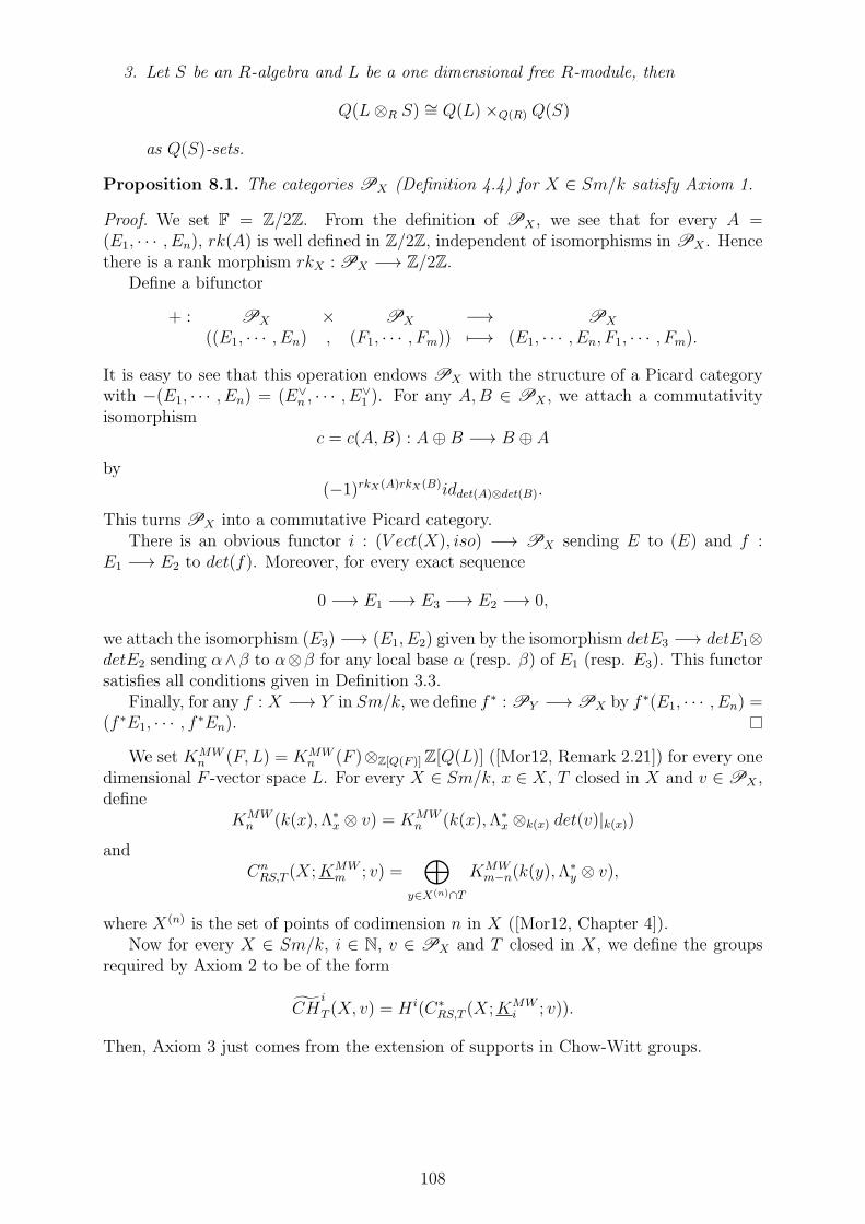
3. Let S be an R-algebra and L be a one dimensional free R-module, then
Q(L⊗R S) ∼= Q(L)×Q(R) Q(S)
as Q(S)-sets.
Proposition 8.1. The categories PX (Definition 4.4) for X ∈ Sm/k satisfy Axiom 1.
Proof. We set F = Z/2Z. From the definition of PX , we see that for every A =(E1, · · · , En), rk(A) is well defined in Z/2Z, independent of isomorphisms in PX . Hencethere is a rank morphism rkX : PX −→ Z/2Z.
Define a bifunctor
+ : PX × PX −→ PX
((E1, · · · , En) , (F1, · · · , Fm)) 7−→ (E1, · · · , En, F1, · · · , Fm).
It is easy to see that this operation endows PX with the structure of a Picard categorywith −(E1, · · · , En) = (E∨
n , · · · , E∨1 ). For any A,B ∈ PX , we attach a commutativity
isomorphismc = c(A,B) : A⊕ B −→ B ⊕ A
by(−1)rkX(A)rkX(B)iddet(A)⊗det(B).
This turns PX into a commutative Picard category.There is an obvious functor i : (V ect(X), iso) −→ PX sending E to (E) and f :
E1 −→ E2 to det(f). Moreover, for every exact sequence
0 −→ E1 −→ E3 −→ E2 −→ 0,
we attach the isomorphism (E3) −→ (E1, E2) given by the isomorphism detE3 −→ detE1⊗detE2 sending α∧β to α⊗β for any local base α (resp. β) of E1 (resp. E3). This functorsatisfies all conditions given in Definition 3.3.
Finally, for any f : X −→ Y in Sm/k, we define f ∗ : PY −→PX by f ∗(E1, · · · , En) =(f ∗E1, · · · , f
∗En).
We set KMWn (F, L) = KMW
n (F )⊗Z[Q(F )]Z[Q(L)] ([Mor12, Remark 2.21]) for every onedimensional F -vector space L. For every X ∈ Sm/k, x ∈ X, T closed in X and v ∈PX ,define
KMWn (k(x),Λ∗
x ⊗ v) = KMWn (k(x),Λ∗
x ⊗k(x) det(v)|k(x))
andCnRS,T (X;KMW
m ; v) =⊕
y∈X(n)∩T
KMWm−n(k(y),Λ
∗y ⊗ v),
where X(n) is the set of points of codimension n in X ([Mor12, Chapter 4]).Now for every X ∈ Sm/k, i ∈ N, v ∈ PX and T closed in X, we define the groups
required by Axiom 2 to be of the form
CHi
T (X, v) = H i(C∗RS,T (X;KMW
i ; v)).
Then, Axiom 3 just comes from the extension of supports in Chow-Witt groups.
108

8.1 Operations without Intersection
Lemma 8.3. Let f : X −→ X ′ be a smooth morphism in Sm/k, and let x ∈ X with[k(x) : k(f(x))] <∞. Then we have an isomorphism
Q(Λ∗x)∼= Q(ω∨
X/X′ |k(x))×Q(k(x)) Q(Λ∗f(x) ⊗ k(x))
(the Qs will be ignored in the sequel for convenience).
Proof. If k(x) is separable over k(f(x)), then we have a commutative diagram with exactrows and columns
0 0
ΩX/X′ |k(x)
OO
ΩX/X′ |k(x)
OO
0 // Ωx//
OO
ΩX/k|k(x) //
OO
Ωk(x)/k// 0
0 // Ωf(x) ⊗ k(x) //
OO
ΩX′/k|k(f(x)) ⊗ k(x) //
OO
Ωk(f(x))/k ⊗ k(x) //
∼=
OO
0
0
OO
0
OO
so we have an isomorphism
Λ∗x∼= ωX/X′ |∨k(x) ⊗ (Λ∗
f(x) ⊗ k(x))
which induces an isomorphism
Q(Λ∗x)∼= Q(ωX/X′ |∨k(x))×Q(k(x)) Q(Λ
∗f(x) ⊗ k(x)).
If the field extension is not separable, we only have the horizontal exact sequences and themiddle vertical arrows. But Q(ωk(x)/k) ∼= Q(ωk(f(x))/k ⊗ k(x)) still holds ([Mor12, Lemma4.1]), so we have isomorphisms
Q(Λ∗x)
−→Q(ωk(x)/k)×Q(k(x)) Q(ω∨k(x)/k)×Q(k(x)) Q(Λ
∗x)
−→Q(ωk(x)/k)×Q(k(x)) Q(ω∨X/k|k(x))
−→Q(ωk(x)/k)×Q(k(x)) Q(ω∨X/X′ |k(x))×Q(k(x)) Q(ω
∨X′/k|k(f(x)) ⊗ k(x))
−→Q(ωk(x)/k)×Q(k(x)) Q(ω∨X/X′ |k(x))×Q(k(x)) Q(ω
∨k(f(x))/k ⊗ k(x))×Q(k(x)) Q(Λ
∗f(x) ⊗ k(x))
−→Q(ωk(x)/k)×Q(k(x)) Q(ω∨X/X′ |k(x))×Q(k(x)) Q(ω
∨k(x)/k)×Q(k(x)) Q(Λ
∗f(x) ⊗ k(x))
−→Q(ω∨X/X′ |k(x))×Q(k(x)) Q(Λ
∗f(x) ⊗ k(x)).
This coincides with the isomorphism we obtained in the case of separable field extensionby applying Theorem 3.1, (2) to the digram above.
Lemma 8.4. Let f : X −→ X ′ be a closed immersion in Sm/k and let x ∈ X (so thatk(x) = k(f(x))). Then we have an isomorphism
Λ∗f(x)∼= Λ∗
x ⊗ detN∨X/X′ |k(x).
109

Proof. This follows by the following commutative diagram with exact rows and columns
0 0
0 // Ωx//
OO
ΩX/k|k(x) //
OO
Ωk(x)/k// 0
0 // Ωf(x)//
OO
ΩX′/k|k(f(x)) //
OO
Ωk(f(x))/k// 0
N∨X/X′ |k(x)
OO
N∨X/X′ |k(x)
OO
0
OO
0
OO
Lemma 8.5. Let f : X −→ X ′ be a smooth morphism in Sm/k, and let x ∈ X withcodim(x) = codim(f(x)). Then, we have an isomorphism
Ωx∼= Ωf(x) ⊗k(f(x)) k(x).
Proof. The cotangent mapΩf(x) ⊗k(f(x)) k(x) −→ Ωx
of f is injective and the two vector spaces have the same dimension codim(x).
Lemma 8.6. Let X1, X2 ∈ Sm/k, x1 ∈ X1, x2 ∈ X2 and let y be the generic point ofsome component of x1 × x2. Then we have an isomorphism
Ωy∼= Ωx1 ⊗k(x1) k(y)⊕ Ωx2 ⊗k(x2) k(y).
Proof. We have the following commutative diagram with exact rows and columns (sameif we exchange X1 and X2)
0
0
0
0 // Ωx1 ⊗ k(y) //
p∗1ΩX1/k|k(y) //
q∗1Ωx1/k|k(y) //
0
0 // Ωy//
ΩX1×X2/k|k(y) //
Ωx1×x2/k|k(y) //
0
0 // Ωx2 ⊗ k(y) //
p∗2ΩX2/k|k(y) //
q∗2Ωx2/k|k(y) //
0
0 0, 0
where pi : X1 ×X2 −→ Xi and qi : x1 × x2 −→ xi are the projections and Ωx1×x2/k|k(y) =Ωy/k|k(y).
Definition 8.4. (Axiom 8) Let f : X −→ X ′ be a smooth morphism, and let x ∈ X withcodim(x) = codim(f(x)). For any v ∈PX′, we have an obvious morphism
KMWn (k(f(x)),Λ∗
f(x) ⊗ v) −→ KMWn (k(x),Λ∗
x ⊗ f∗v)
110

by Lemma 8.5. This induces a pull-back morphism ([Fas08, Corollaire 10.4.2])
f ∗ : CHn
T (X′, v) −→ CH
n
f−1(T )(X, f∗(v))
for every T ∈ Zn(X). It is functorial with respect to v.
Remark 8.1. The pull-back along closed immersions is much more difficult and we willdiscuss this in Section 8.2.
The following proposition is obvious.
Proposition 8.2. (Axiom 9) The pull-back between smooth morphisms is functorial andf ∗(1) = 1.
Definition 8.5. (Axiom 11) Let f : X −→ X ′ be a smooth morphism and let C ∈Zi+df (X) be finite over X ′. We define the push-forward (Proposition 8.6)
f∗ : CHi+df
C (X, f ∗v − TX/X′) −→ CHi
f(C)(X′, v)
as the composite for every x ∈ C ∩X(i+df )
KMW0 (k(x),Λ∗
x ⊗ f∗v ⊗ ωX/X′) // KMW
0 (k(x), ω∨X/X′ ⊗ (Λ∗
f(x) ⊗ k(x))⊗ f∗v ⊗ ωX/X′)
Trk(x)k(f(x))
KMW0 (k(f(x)),Λ∗
f(x) ⊗ v)
where the horizontal arrow is induced by Lemma 8.3, while the vertical arrow is the tracemap composed with the isomorphism of virtual vector bundles cancelling the first and lastbundle. The push-forward for smooth morphisms is functorial with respect to v.
It’s clear by definition that Axiom 20 is satisfied.
Definition 8.6. (Axiom 13) Let f : X −→ X ′ be a closed immersion and let C ∈Zi+df (X). We define the push-forward (Proposition 8.7)
f∗ : CHi+df
C (X,NX/X′ + f ∗v) −→ CHi
f(C)(X′, v)
by the isomorphism induced by Lemma 8.4
KMW0 (k(x),Λ∗
x ⊗ detNX/X′ ⊗ f ∗v) // KMW0 (k(f(x)),Λ∗
f(x) ⊗ v)
for every x ∈ C ∩ X(i+df ). The push-forward for closed immersions is functorial withrespect to v.
Remark 8.2. Suppose that f : X −→ X ′ is a morphism of schemes and that C ∈Zi+df (X) is such that C = x for some x ∈ X. Suppose further that C is also closed inX ′. Then, we have an exact sequence
0 −→ TX/X′ |k(x) −→ Ω∗x −→ Ω∗
f(x) −→ 0;
if f is a closed immersion, we have an exact sequence
0 −→ Ω∗x −→ Ω∗
f(x) −→ NX/X′ |k(x) −→ 0.
111

So, we can identify Ω∗x with Nx/X |k(x) since the latter satisfies the same exact sequences
when C is smooth. Hence in the context above, the push-forward associated to f withsupport C is completely determined by the composite
NC/X + f ∗v|C − TX/X′ |C −→ TX/X′ |C +NC/Y + f ∗v|C − TX/X′ |C −→ NC/Y + f ∗v|C
in case f is smooth and by the isomorphism
NC/X +NX/X′ |C + f ∗v|C −→ NC/Y + f ∗v|C
if f is a closed immersion.This inspires us to convert equations of twisted Chow-Witt groups into equations of
virtual objects. Then use the method described in Chapter 3. This is the main idea wewill use in this chapter.
We now explain the differentials in the Rost-Schmid complex. Suppose thatX ∈ Sm/kand that Y = y for some y ∈ X. Let further Z = z for some z ∈ Y (1) and v ∈ PX . Wenow define the differential
∂yz : KMWn (k(y),Λ∗
y ⊗ v) −→ KMWn−1 (k(z),Λ
∗z ⊗ v).
Suppose at first that Y is normal. Then the exact sequence
IY /I2Y −→ ΩX/k|Y −→ ΩY/k −→ 0
is also left exact at the stalk of z, and we have a commutative diagram with exact rows
0 // IY /I2Y |k(z) //
i
ΩX/k|k(z) // ΩY/k|k(z) //
0
0 // IZ/I2Z |k(z) // ΩX/k|k(z) // ΩZ/k|k(z) // 0.
The map i is injective with cokernel mz/m2z, where mz is the maximal ideal of OY,z. Thus,
we have an exact sequence
0 −→ (mz/m2z)
∨ −→ (IZ/I2Z)
∨|k(z) −→ (IY /I2Y )
∨|k(z) −→ 0.
Now choose a free basis a of (IY /I2Y )
∨z , e of (mz/m
2z)
∨ and t of det(v)z. Hence a is alsoa free basis of Ω∗
y = (IY /I2Y )
∨|k(y) and (e, a) is a free basis of Ω∗z = (IZ/I
2Z)
∨|k(z) by thesequence above. We define the map ∂ by
KMWn (k(y),Λ∗
y ⊗ v) −→ KMWn−1 (k(z),Λ
∗z ⊗ v)
s⊗ a⊗ t 7−→ ∂ez(s)⊗ (e ∧ a)⊗ t,
where ∂ez is the usual partial map for Milnor-Witt groups. This map is independent ofthe choice of a, e, t.
In general, let Y be the normalization of Y with morphism π : Y −→ Y and letzi = π−1(z). We have an isomorphism (the same for z)
Λ∗y∼= ωk(y)/k ⊗ ω
∨X/k|k(y).
Now fix zi. We find that ΩOY ,zi
/k satisfies
ΩOY ,zi
/k ⊗ k(y) = Ωk(y)/k.
112

Also, we have an exact sequence
0 −→ mzi/m2zi−→ ΩO
Y ,zi/k ⊗ k(zi) −→ Ωk(zi)/k −→ 0.
So, choose a free basis ei of (mzi/m2zi)∨, ci of ΩO
Y ,zi/k, d of (Ω∨
X/k)z and l of det(v)z. We
define ∂i by the following composite
KMWn (k(y),Λ∗
y ⊗ v)
−→KMWn (k(y), ωk(y)/k ⊗ ω
∨X/k ⊗ v)
−→KMWn−1 (k(zi), (mzi/m
2zi)∨ ⊗ (ωO
Y ,zi/k ⊗ k(zi))⊗k(zi) (ω
∨X/k|k(z) ⊗k(z) v|k(z)))
−→KMWn−1 (k(zi), ωk(zi)/k ⊗k(zi) (ω
∨X/k|k(z) ⊗k(z) v|k(z)))
−→KMWn−1 (k(zi), (ωk(z)/k ⊗ k(zi))⊗k(zi) (ω
∨X/k|k(z) ⊗k(z) v|k(z)))
−→KMWn−1 (k(zi), (ωk(z)/k ⊗k(z) ω
∨X/k|k(z) ⊗k(z) v|k(z))⊗k(z) k(zi))
−→KMWn−1 (k(z), ωk(z)/k ⊗k(z) ω
∨X/k|k(z) ⊗k(z) v|k(z))
−→KMWn−1 (k(z),Λ
∗z ⊗ v),
where the second arrow is defined by
s⊗ ci ⊗ d⊗ l 7−→ ∂eizi (s)⊗ ei ⊗ (ci ⊗ 1)⊗ d⊗ l,
which is independent of the choice of ei. Then we define ∂yz =∑∂i. This definition
coincides with the definition just given when Y is normal by applying Theorem 3.1, (4)to the following commutative diagram with exact columns and rows
0
0
0 // TZ/k|k(z) // TY/k|k(z)
// (mz/m2z)
∨ //
0
0 // TZ/k|k(z) // TX/k|k(z) //
(IZ/I2Z)
∨|k(z) //
0
(IY /I2Y )
∨|k(z)
(IY /I2Y )
∨|k(z)
0 0.
Remark 8.3. Here we would like to treat a kind of linearity of ∂yz . Let s ∈ KMWn (k(y),Λ∗
y⊗v).
1. Suppose that f ∈ O∗Y,z and that n = 0, we want to show that
∂yz ([f ]s) = [f ]∂yz (s).
It suffices to show the formula for each ∂i. We see that ∂i = Trk(zi)k(z) ∂
eizi
and
∂eizi ([f ]s) = ǫ[f ]∂eizi (s). Suppose that ∂eizi (s) =< a > η. Then
Trk(zi)k(z) (ǫ[f ] < a > η)
=Trk(zi)k(z) ((< f > − < 1 >) < a >)
=(< f > − < 1 >)Trk(zi)k(z) (< a >)
=[f ]Trk(zi)k(z) (< a > η).
Then the claim is proved.
113

2. If we have another line bundle M over X and m is a free basis of Mz (so it’s alsoa free basis of My), we have
∂yz (s⊗m) = ∂yz (s)⊗m.
We note nevertheless that this doesn’t hold for a general free basis of My. indeed,if we replace m by λ ·m, where λ ∈ k(y)∗, then λ plays a role in the computation ofthe residue maps.
Remark 8.4. It’s obvious that any morphism v1 −→ v2 in PX will induce an isomor-phism between the corresponding Rost-Schmid complexes.
Definition 8.7. ([CF18]) Let Xa ∈ Sm/k and let xa ∈ Xa for a = 1, 2. Let y be thegeneric point of some component of x1 × x2. For every sa ∈ K
MWn (k(xa),Λ
∗xa ⊗ va), we
define
s1 × s2 =∑
y
c(p∗1(v1), p∗2(Λ
∗x2))(p∗1(s1)⊗ p
∗2(s2)) ∈ ⊕yK
MWn+m(k(y),Λ
∗y ⊗ (p∗1(v1) + p∗2(v2))),
where pi : y −→ xi is the projection (note the use of Lemma 8.6). It is called the exteriorproduct between s1 and s2. The exterior product is functorial with respect to twists andextension of supports.
We will denote p∗1(v1) + p∗2(v2) by v1 × v2 for convenience.Now we focus of a special case of the proof that the right exterior product with an
element in Chow-Witt groups (with support) is a chain complex map between Rost-Schmid complexes, while the left exterior product is not.
Proposition 8.3. Let X,X ′ ∈ Sm/k, v ∈PX , v′ ∈PX′ and let Y ∈ Zi(X), T ∈ Zj(X ′)
be smooth. Suppose that β ∈ CHj
T (X′, v′). Then the following diagram commutes
⊕s∈(Y×T )(0)KMWn (k(s),Λ∗
s ⊗ (v × v′)) ∂ // ⊕u∈(X×X′)(i+j+1)KMWn−1 (k(u),Λ
∗u ⊗ (v × v′))
⊕y∈Y (0)KMWn (k(y),Λ∗
y ⊗ v)∂ //
×β
OO
⊕z∈Y ∩X(i+1)KMWn−1 (k(z),Λ
∗z ⊗ v)
×β
OO.
That is, for every β ∈ CHj
T (X′, v′) and α ∈ ⊕y∈Y (0)KMW
n (k(y),Λ∗y ⊗ v), we have
∂(α× β) = ∂(α)× β.
Moreover, we have∂(β × α) =< −1 >j+rkX′ (v′) β × ∂(α).
Proof. We may assume that Y and T are irreducible. We check the commutativity afterprojecting to each u ∈ (X×X ′)(i+j+1). It suffices to let u be a generic point of z×T , wherez ∈ Y ∩X(i+1), since otherwise both terms vanish. Set Z = z. We have a commutative
114

diagram with exact columns and rows (we write X × Y by XY for short)
0
0
NZT/Y T
NZT/Y T
0 // NZT/XT//
NZT/XX′
// NXT/XX′ |ZT //
∼=
0
0 // NY T/XT |ZT //
NY T/XX′ |ZT //
NY T/Y X′ |ZT // 0
0 0.
We have projection maps p1 : ZT −→ Z and p2 : ZT −→ T . By Theorem 3.1, (1), wehave a commutative diagram
p∗1(NZ/Y +NY/X |Z + v|Z) + p∗2(NT/X′ + v′|T ) //
p∗1(NZ/Y ) +NY T/XX′ |ZT + p∗1(v|Z) + p∗2(v′|T )
p∗1(NZ/X + v|Z) + p∗2(NT/X′ + v′|T )
NZT/Y T +NY T/XX′ |ZT + p∗1(v|Z) + p∗2(v′|T )
NZT/XT + p∗1(v|Z) +NY T/Y X′ |ZT + p∗2(v′|T ) // NZT/XX′ + p∗1(v|Z) + p∗2(v
′|T ),
which gives the first equation. For the second one, we compute directly using the firstequation using Proposition 8.4 (which still holds in this context):
∂(β × α)
=∂(< −1 >(i+rkX(v))(j+rkX′ (v′)) c(q∗1v1, q∗2v2)(α× β))
= < −1 >(i+rkX(v))(j+rkX′ (v′)) c(q∗1v1, q∗2v2)(∂(α× β))
= < −1 >(i+rkX(v))(j+rkX′ (v′)) c(q∗1v1, q∗2v2)(∂(α)× β)
= < −1 >j+rkX′ (v′) β × ∂(α),
where q1, q2 are the respective projections of X ×X ′ on the corresponding factor.
Definition 8.8. The exterior product of Definition 8.7 induces a pairing
CHn1
T1(X1, v1)× CH
n2
T2(X2, v2) −→ CH
n1+n2
T1×T2(X1 ×X2, v1 × v2)
for every Xa ∈ Sm/k, Ta ∈ Zna(Xa) smooth and va ∈ PXa for a = 1, 2 by Proposition
8.3. It’s called the exterior product between Chow-Witt groups.
Proposition 8.4. (Axiom 5 and 6) In the context above, the exterior product is associativeand satisfies
s1 × s2 =< −1 >(codim(x1)+rkX1
(v1))(codim(x2)+rkX2(v2)) c(p∗2(v2), p
∗1(v1))(s2 × s1)
where sa ∈ CHna
Ta(Xa, va).
Proof. Associativity comes from Definition 3.3, (3) and the second statement follows fromthe definition of the commutativity isomorphism in Proposition 8.1.
115

Proposition 8.5. (Axiom 10) Let fa : Ya −→ Xa be smooth morphisms in Sm/k fora = 1, 2. Then, we have
(f1 × f2)∗(s1 × s2) = f ∗
1 (s1)× f∗2 (s2).
Proof. This follows from Lemma 8.5 and Lemma 8.6.
Now, we would like to prove a special case that the the push-forwards defined inDefinition 8.5 and Definition 8.6 form a chain complex morphism between Rost-Schmidcomplexes, just to explain how to treat the twists.
Proposition 8.6. Suppose that Z ⊆ Y ⊆ X are schemes with X and Y smooth. Supposethat Y = y in X and that Z = z in Y for some z ∈ Y (1). Suppose moreover thatf : X −→ X ′ is a smooth morphism, that v ∈ PX′ and that Y is also a closed subset ofX ′. Then we have a commutative diagram
KMWn (k(y),Λ∗
y ⊗ f∗v ⊗ ωX/X′) ∂ //
f∗
KMWn−1 (k(z),Λ
∗z ⊗ f
∗v ⊗ ωX/X′)
f∗
KMWn (k(f(y)),Λ∗
f(y) ⊗ v)∂ // KMW
n−1 (k(f(z)),Λ∗f(z) ⊗ v).
Proof. We have the following commutative diagram with exact rows and columns
0
0
NZ/Y
NZ/Y
0 // TX/X′ |Z // NZ/X
// NZ/X′//
0
0 // TX/X′ |Z // NY/X |Z //
NY/X′ |Z //
0
0 0.
Now the statement is to prove that the following diagram commutes
NZ/Y +NY/X |Z + f ∗v|Z − TX/X′ |Z //
NZ/Y + TX/X′ |Z +NY/X′ |Z + f ∗v|Z − TX/X′ |Z
NZ/X + f ∗v|Z − TX/X′ |Z
NZ/Y +NY/X′ |Z + f ∗v|Z
TX/X′ |Z +NZ/X′ + f ∗v|Z − TX/X′ |Z // NZ/X′ + f ∗v|Z .
We have the following commutative diagrams
TX/X′ |Z +NZ/X′ + f ∗v|Z − TX/X′ |Z // NZ/X′ + f ∗v|Z
TX/X′ |Z +NZ/Y +NY/X′ |Z + f ∗v|Z − TX/X′ |Z //
OO
NZ/Y +NY/X′ |Z + f ∗v|Z
OO
116
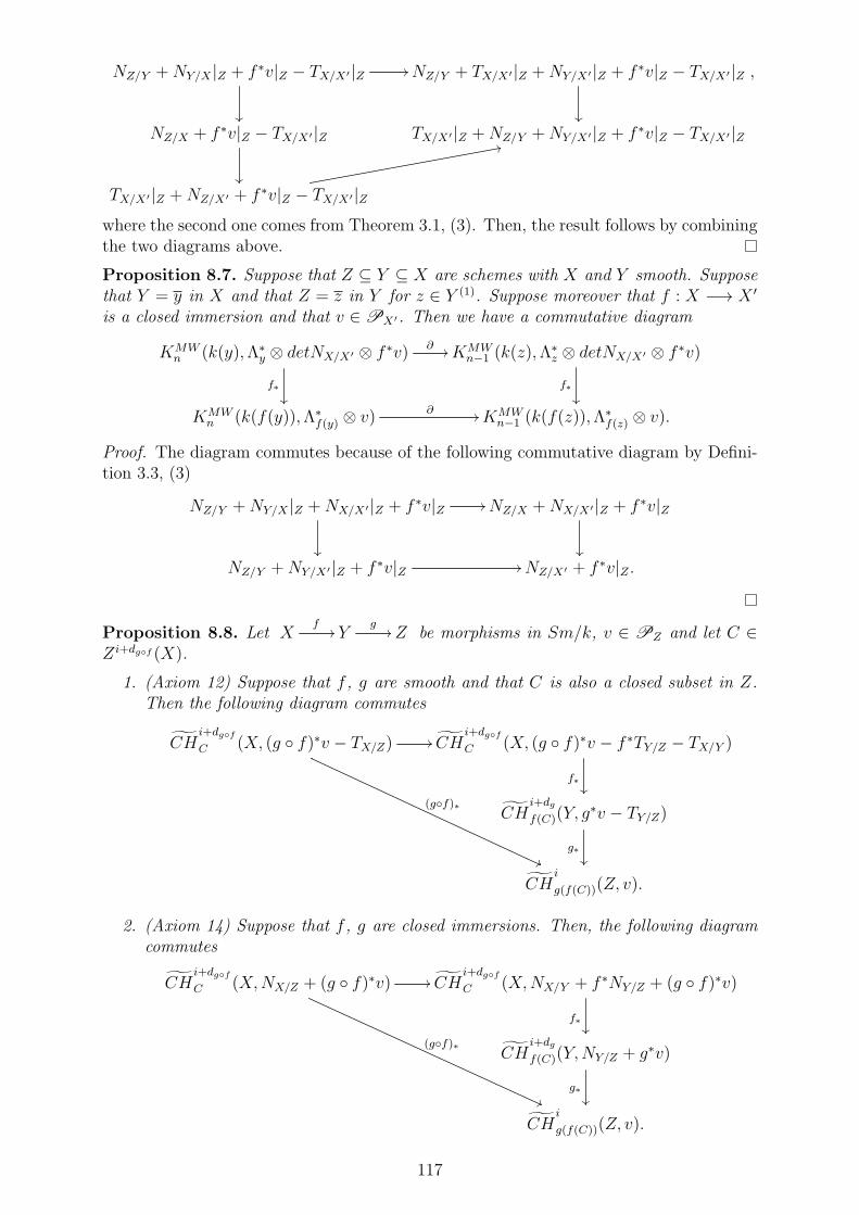
NZ/Y +NY/X |Z + f ∗v|Z − TX/X′ |Z //
NZ/Y + TX/X′ |Z +NY/X′ |Z + f ∗v|Z − TX/X′ |Z
NZ/X + f ∗v|Z − TX/X′ |Z
TX/X′ |Z +NZ/Y +NY/X′ |Z + f ∗v|Z − TX/X′ |Z
TX/X′ |Z +NZ/X′ + f ∗v|Z − TX/X′ |Z
22
,
where the second one comes from Theorem 3.1, (3). Then, the result follows by combiningthe two diagrams above.
Proposition 8.7. Suppose that Z ⊆ Y ⊆ X are schemes with X and Y smooth. Supposethat Y = y in X and that Z = z in Y for z ∈ Y (1). Suppose moreover that f : X −→ X ′
is a closed immersion and that v ∈PX′. Then we have a commutative diagram
KMWn (k(y),Λ∗
y ⊗ detNX/X′ ⊗ f ∗v) ∂ //
f∗
KMWn−1 (k(z),Λ
∗z ⊗ detNX/X′ ⊗ f ∗v)
f∗
KMWn (k(f(y)),Λ∗
f(y) ⊗ v)∂ // KMW
n−1 (k(f(z)),Λ∗f(z) ⊗ v).
Proof. The diagram commutes because of the following commutative diagram by Defini-tion 3.3, (3)
NZ/Y +NY/X |Z +NX/X′ |Z + f ∗v|Z //
NZ/X +NX/X′ |Z + f ∗v|Z
NZ/Y +NY/X′ |Z + f ∗v|Z // NZ/X′ + f ∗v|Z .
Proposition 8.8. Let Xf
// Yg
// Z be morphisms in Sm/k, v ∈ PZ and let C ∈Zi+dgf (X).
1. (Axiom 12) Suppose that f , g are smooth and that C is also a closed subset in Z.Then the following diagram commutes
CHi+dgf
C (X, (g f)∗v − TX/Z) //
(gf)∗
((
CHi+dgf
C (X, (g f)∗v − f ∗TY/Z − TX/Y )
f∗
CHi+dg
f(C)(Y, g∗v − TY/Z)
g∗
CHi
g(f(C))(Z, v).
2. (Axiom 14) Suppose that f , g are closed immersions. Then, the following diagramcommutes
CHi+dgf
C (X,NX/Z + (g f)∗v) //
(gf)∗
((
CHi+dgf
C (X,NX/Y + f ∗NY/Z + (g f)∗v)
f∗
CHi+dg
f(C)(Y,NY/Z + g∗v)
g∗
CHi
g(f(C))(Z, v).
117

3. (Axiom 19, (1)) Suppose that f is a closed immersion, that g and g f are smoothand that C is also a closed subset of Z. Then the following diagram commutes
CHi+dgf
C (X,NX/Y + f ∗g∗v − f ∗TY/Z)
f∗
// CHi+dgf
C (X, f ∗g∗v +NX/Y − f∗TY/Z)
CHi+dg
f(C)(Y, g∗v − TY/Z)
g∗
CHi+dgf
C (X, f ∗g∗v − TX/Z)
(gf)∗
ss
CHi
g(f(C))(Z, v).
4. (Axiom 19, (2)) Suppose that g is smooth, and that f and gf are closed immersions.Then the following diagram commutes
CHi+dgf
C (X,NX/Y + f ∗g∗v − f ∗TY/Z)
f∗
// CHi+dgf
C (X,−f ∗TY/Z +NX/Y + f ∗g∗v)
CHi+dg
f(C)(Y, g∗v − TY/Z)
g∗
CHi+dgf
C (X,NX/Z + f ∗g∗v)
(gf)∗
rr
CHi
g(f(C))(Z, v).
Proof. 1. This follows from the following commutative diagram
NC/X + f ∗g∗v|C − TX/Z |C //
NC/X + f ∗g∗v|C − f∗TY/Z |C − TX/Y |C
TX/Y |C +NC/Y + f ∗g∗v|C − f∗TY/Z |C − TX/Y |C
NC/Y + f ∗g∗v|C − f∗TY/Z |C
f ∗TY/Z |C +NC/Z + f ∗g∗v|C − f∗TY/Z |C
TX/Z |C +NC/Z + f ∗g∗v|C − TX/Z |C // NC/Z + f ∗g∗v|C
using Definition 3.3, (3).
2. Essentially the same as in (1).
118

3. We are going to prove that the following diagram commutes
NC/X +NX/Y |C + f ∗g∗v|C − f∗TY/Z |C //
NC/X + f ∗g∗v|C +NX/Y |C − f∗TY/Z |C
NC/Y + f ∗g∗v|C − f∗TY/Z |C
NC/X + f ∗g∗v|C +NX/Y |C −NX/Y |C − TX/Z |C
f ∗TY/Z |C +NC/Z + f ∗g∗v|C − f∗TY/Z |C
NC/X + f ∗g∗v|C − TX/Z |C
NC/Z + f ∗g∗v|C TX/Z |C +NC/Z + f ∗g∗v|C − TX/Z |Coo
.
Let A = TX/Z |C+NX/Y |C+NC/Z+f∗g∗v|C−NX/Y |C−TX/Z |C . We have commutative
diagrams
f ∗TY/Z |C +NC/Z + f ∗g∗v|C − f∗TY/Z |C //
A
NC/Z + f ∗g∗v|C // TX/Z |C +NC/Z + f ∗g∗v|C − TX/Z |C
NC/X +NX/Y |C + f ∗g∗v|C −NX/Y |C − TX/Z |C
++NC/X + f ∗g∗v|C − TX/Z |C
A
ss
TX/Z |C +NC/Z + f ∗g∗v|C − TX/Z |C .
Furthermore, there is a commutative diagram with exact rows and columns
0
0
0 // TX/Z |C //
NC/X
// NC/Z// 0
0 // f ∗TY/Z |C //
NC/Y//
NC/Z// 0
NX/Y |C
NX/Y |C
0 0
and by Theorem 3.1, (2), we have a commutative diagram
NC/X +NX/Y |C + f ∗g∗v|C − f∗TY/Z |C //
NC/X +NX/Y |C + f ∗g∗v|C − f∗TY/Z |C
NC/Y + f ∗g∗v|C − f∗TY/Z |C
TX/Z |C +NC/Z |C +NX/Y |C + f ∗g∗v|C − f∗TY/Z |C
f ∗TY/Z |C +NC/Z + f ∗g∗v|C − f∗TY/Z |C // A.
The proof follows easily.
119
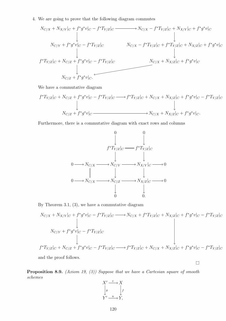
4. We are going to prove that the following diagram commutes
NC/X +NX/Y |C + f ∗g∗v|C − f∗TY/Z |C //
NC/X − f∗TY/Z |C +NX/Y |C + f ∗g∗v|C
NC/Y + f ∗g∗v|C − f∗TY/Z |C
NC/X − f∗TY/Z |C + f ∗TY/Z |C +NX/Z |C + f ∗g∗v|C
f ∗TY/Z |C +NC/Z + f ∗g∗v|C − f∗TY/Z |C
NC/X +NX/Z |C + f ∗g∗v|C
rr
NC/Z + f ∗g∗v|C .
We have a commutative diagram
f ∗TY/Z |C +NC/Z + f ∗g∗v|C − f∗TY/Z |C //
f ∗TY/Z |C +NC/X +NX/Z |C + f ∗g∗v|C − f∗TY/Z |C
NC/Z + f ∗g∗v|C // NC/X +NX/Z |C + f ∗g∗v|C .
Furthermore, there is a commutative diagram with exact rows and columns
0
0
f ∗TY/Z |C
f ∗TY/Z |C
0 // NC/X// NC/Y
// NX/Y |C //
0
0 // NC/X// NC/Z
//
NX/Z |C //
0
0 0.
By Theorem 3.1, (3), we have a commutative diagram
NC/X +NX/Y |C + f ∗g∗v|C − f∗TY/Z |C //
NC/X + f ∗TY/Z |C +NX/Z |C + f ∗g∗v|C − f∗TY/Z |C
NC/Y + f ∗g∗v|C − f∗TY/Z |C
f ∗TY/Z |C +NC/Z + f ∗g∗v|C − f∗TY/Z |C // f ∗TY/Z |C +NC/X +NX/Z |C + f ∗g∗v|C − f
∗TY/Z |C
and the proof follows.
Proposition 8.9. (Axiom 19, (3)) Suppose that we have a Cartesian square of smoothschemes
X ′ v //
g
X
f
Y ′ u // Y,
120

where u is smooth and f is a closed immersion: Let s ∈ PY and let C ∈ Zn+df+dv(X ′)be also closed in Y . Then the following diagram commutes
CHn+df+dv
C (X ′, NX′/Y ′ + g∗u∗s− g∗TY ′/Y )g∗
//
CHn+du
g(C) (X, u∗s− TY ′/Y )
u∗
CHn+df+dv
C (X ′, v∗NX/Y + u∗f ∗s− TX′/X)
v∗
CHn
u(g(C))(Y, s)
CHn+df
v(C) (X,NX/Y + f ∗s).
f∗
33
Proof. We are going to show that the following diagram commutes
NC/X′ +NX′/Y ′ |C + g∗u∗s|C − g∗TY ′/Y |C
// NC/Y ′ + g∗u∗s|C − g∗TY ′/Y |C
NC/X′ + v∗NX/Y |C + g∗u∗s|C − TX′/X |C
g∗TY ′/Y |C +NC/Y + g∗u∗s|C − g∗TY ′/Y |C
TX′/X |C +NC/X + v∗NX/Y |C + g∗u∗s|C − TX′/X |C
NC/Y + g∗u∗s|C
NC/X + v∗NX/Y |C + g∗u∗s|C .
22
We have a commutative diagram with exact rows and columns
0
0
TX′/X |C
∼= // g∗TY ′/Y |C
0 // NC/X′//
NC/Y ′
// NX′/Y ′ |C //
∼=
0
0 // NC/X//
NC/Y//
v∗NX/Y |C // 0
0 0.
So, we have a commutative diagram by Theorem 3.1, (1)
NC/Y ′//
NC/X′ +NX′/Y ′ |C
g∗TY ′/Y |C +NC/Y
TX′/X |C +NC/X +NX′/Y ′ |C
g∗TY ′/Y |C +NC/X + v∗NX/Y |C .
33
Then the statement follows easily from the data above.
121

Proposition 8.10. Suppose that we have a Cartesian square of smooth schemes
X ′ v //
g
X
f
Y ′ u // Y.
1. (Axiom 15) Suppose that f , u are smooth, that s ∈PY and that C ∈ Zn+df (X) isa closed subset of Y . Then the following diagram commutes
CHn+df
C (X, f ∗s− TX/Y )f∗
//
v∗
CHn
f(C)(Y, s)
u∗
CHn+df
v−1(C)(X′, v∗f ∗s− v∗TX/Y )
g∗// CH
n
g(v−1(C))(Y′, u∗s).
2. (Axiom 16) Suppose that f is a closed immersion, that s ∈ PY and that C ∈Zn+df (X). Suppose moreover that u is smooth. Then the following diagram com-mutes
CHn+df
C (X,NX/Y + f ∗s)f∗
//
v∗
CHn
f(C)(Y, s)
u∗
CHn+df
v−1(C)(X′, v∗NX/Y + v∗f ∗s)
g∗// CH
n
g(v−1(C))(Y′, u∗s).
Proof. 1. We have a commutative diagram by functoriality of v∗ with respect to twists
NC/X + f ∗v|C − TX/Y |C //
TX/Y |C +NC/Y + f ∗s|C − TX/Y |C
Nv−1(C)/X′ + v∗f ∗s|v−1(C) − TX′/Y ′ |v−1(C)
NC/Y + f ∗s|C
TX′/Y ′ |v−1(C) +Nv−1(C)/Y ′ + v∗f ∗s|v−1(C) − TX′/Y ′ |v−1(C)// Nv−1(C)/Y ′ + f ∗s|v−1(C).
2. We have a commutative diagram by functoriality of v∗ with respect to twists
NC/X +NX/Y |C + f ∗s|C //
NC/Y + f ∗s|C
Nv−1(C)/X′ +NX′/Y ′ |v−1(C) + v∗f ∗s|v−1(C)// Nv−1(C)/Y ′ + v∗f ∗s|v−1(C).
Proposition 8.11. 1. (Axiom 17) Suppose that f : X −→ Y is a smooth morphism inSm/k, that v ∈PY and that C ∈ Zn+df (X) is a smooth closed subset of Y . Then,for any Z ∈ Sm/k, any v′ ∈ PZ and any D ∈ Zm(Z), the following diagramscommute
CHn+df
C (X, f ∗v − TX/Y )× CHm
D(Z, v′)
×//
f∗×id
CHn+df+m
C×D (X × Z, (f ∗v − TX/Y )× v′)
c
CHn+df+m
C×D (X × Z, (f ∗v × v′)− TX×Z/Y×Z)
(f×id)∗
CHn
f(C)(Y, v)× CHm
D(Z, v′)
×// CH
n+m
f(C)×D(Y × Z, v × v′)
122

CHm
D(Z, v′)× CH
n+df
C (X, f ∗v − TX/Y )×
//
id×f∗
CHn+df+m
D×C (Z ×X, v′ × (f ∗v − TX/Y ))
(id×f)∗
CHm
D(Z, v′)× CH
n
f(C)(Y, v)×
// CHn+m
D×f(C)(Z × Y, v′ × v).
2. (Axiom 18) Suppose that f : X −→ Y is a closed immersion in Sm/k, that v ∈PY
and that C is a smooth closed subset of X. Then for any Z ∈ Sm/k, any v′ ∈PZ
and any D ∈ Zm(Z), the following diagrams commute
CHn+df
C (X,NX/Y + f ∗v)× CHm
D(Z, v′)
×//
f∗×id
CHn+df+m
C×D (X × Z, (NX/Y + f ∗v)× v′)
(f×id)∗
CHn
f(C)(Y, v)× CHm
D(Z, v′)
×// CH
n+m
f(C)×D(Y × Z, v × v′)
CHm
D(Z, v′)× CH
n+df
C (X,NX/Y + f ∗v)×
//
id×f∗
CHn+df+m
D×C (Z ×X, v′ × (NX/Y + f ∗v))
c
CHn+df+m
D×C (Z ×X, (v′ × f ∗v) +NX×Z/Y×Z)
(id×f)∗
CHm
D(Z, v′)× CH
n
f(C)(Y, v)×
// CHn+m
D×f(C)(Z × Y, v′ × v).
Proof. We have projections p1 : C ×D −→ C and p2 : C ×D −→ D.
1. For the first diagram, we are going to prove that the following diagram commutes
(NC/X + f ∗v|C − TX/Y |C , ND/Z + v′|D) //
f∗
p∗1(NC/X + f ∗v|C − TX/Y |C) + p∗2(ND/Z + v′|D)
(NC/Y + f ∗v|C , ND/Z + v′|D)
NC×D/X×Z + p∗1(f∗v|C) + p∗2(v
′|D)− TX×Z/Y×Z |C×D
(f×id)∗
p∗1(NC/Y + f ∗v|C) + p∗2(ND/Z + v′|D) // NC×D/Y×Z + p∗1(f∗v|C) + p∗2(v
′|D).
We have a commutative diagram
(NC/X + f ∗v|C − TX/Y |C , ND/Z + v′|D) //
f∗
p∗1(NC/X + f ∗v|C − TX/Y |C) + p∗2(ND/Z + v′|D)
p∗1(f∗)+p∗
2(id)
uu
(NC/Y + f ∗v|C , ND/Z + v′|D)
p∗1(NC/Y + f ∗v|C) + p∗2(ND/Z + v′|D)
and then we just have to show the following diagram commutes
p∗1(NC/X + f ∗v|C − TX/Y |C) + p∗2(ND/Z + v′|D)
p∗1(f∗)+p
∗
2(id)
ww
NC×D/X×Z + p∗1(f∗v|C) + p∗2(v
′|D)− TX×Z/Y×Z |C×D
(f×id)∗
p∗1(NC/Y + f ∗v|C) + p∗2(ND/Z + v′|D) // NC×D/Y×Z + p∗1(f∗v|C) + p∗2(v
′|D).
123

This follows from Theorem 3.1, (1) and the following commutative diagram withexact rows and columns
0
0
p∗1(TX/Y |C)
∼= // TX×Z/Y×Z |C×D
0 // p∗1NC/X//
NC×D/X×Z
// p∗2ND/Z// 0
0 // p∗1NC/Y//
NC×D/Y×Z//
p∗2ND/Z// 0
0 0.
For the second diagram, we suppose that α ∈ CHn+df
C (X, f ∗v − TX/Y ) and that
β ∈ CHm
D(Z, v′). Moreover, we have a commutative diagram
X
f
X × Zp1
oop2
//
f×id
D
Y Y × Z.q1
oo
q2
;;
Then
(id× f)∗(β × α)
=(f × id)∗(< −1 >(n+rkY (v))(m+rkZ(v′)) c(p∗1(f
∗v − TX/Y ), p∗2(v
′))(α× β))
by Proposition 8.4
= < −1 >(n+rkY (v))(m+rkZ(v′)) (f × id)∗(c(p∗1(f
∗v − TX/Y ), p∗2(v
′))(α× β))
= < −1 >(n+rkY (v))(m+rkZ(v′)) (f × id)∗((c(p∗1(f
∗v), p∗2(v′)) c(−p∗1TX/Y , p
∗2(v
′)))(α× β))
= < −1 >(n+rkY (v))(m+rkZ(v′)) c(q∗1(v), q∗2(v
′))((f × id)∗(c(−p∗1TX/Y , p
∗2(v
′))(α× β)))
by functoriality of push-forwards with respect to twists
= < −1 >(n+rkY (v))(m+rkZ(v′)) c(q∗1(v), q∗2(v
′))(f∗(α)× β))
by the first diagram
=β × f∗(α)
by Proposition 8.4.
2. For the first diagram, we are going to prove that the following diagram commutes
(NC/X +NX/Y |C + f ∗v|C , ND/Z + v′) //
p∗1(NC/X +NX/Y |C + f ∗v|C) + p∗2(ND/Z + v′)
(NC/Y + f ∗v|C , ND/Z + v′)
NC×D/X×Z +NX×Z/Y×Z |C×D + p∗1(f∗v|C) + p∗2(v
′)
p∗1(NC/Y + f ∗v|C) + p∗2(ND/Z + v′) // NC×D/Y×Z + p∗1(f∗v|C) + p∗2(v
′).
124

We have a commutative diagram
(NC/X +NX/Y |C + f ∗v|C , ND/Z + v′) //
p∗1(NC/X +NX/Y |C + f ∗v|C) + p∗2(ND/Z + v′)
p∗1(f∗)+p∗
2(id)
uu
(NC/Y + f ∗v|C , ND/Z + v′)
p∗1(NC/Y + f ∗v|C) + p∗2(ND/Z + v′).
Hence we just have to show that the following diagram commutes
p∗1(NC/X +NX/Y |C + f ∗v|C) + p∗2(ND/Z + v′)
p∗1(f∗)+p
∗
2(id)
xx
NC×D/X×Z +NX×Z/Y×Z |C×D + p∗1(f∗v|C) + p∗2(v
′)
p∗1(NC/Y + f ∗v|C) + p∗2(ND/Z + v′) // NC×D/Y×Z + p∗1(f∗v|C) + p∗2(v
′).
This follows fromTheorem 3.1, (2) together with the following commutative diagramwith exact rows and columns
0
0
0 // p∗1NC/X//
NC×D/X×Z
// p∗2ND/Z// 0
0 // p∗1NC/Y//
NC×D/Y×Z//
p∗2ND/Z// 0
p∗1(NX/Y |C)
∼= // NX×Z/Y×Z |C×D
0 0.
The second diagram follows by the same method as in the proof of the seconddiagram of (1).
8.2 Intersection with Divisors
In this section, we discuss a special case of intersection, namely pull-backs along a divi-sor with smooth support. The constructions here basically come from [CF18], but thetreatments of push-forwards are possibly different.
Definition 8.9. Let X ∈ Sm/k and let D = (Ui, fi) be a Cartier divisor on X. Suppose
that C ∈ Zn(X), s ∈ CHn
C(X, v) and that dim(C ∩ |D|) < dim(C). Let
s =∑
a
sa ⊗ ua ⊗ va ∈ ⊕ya∈X(n)KMW0 (k(ya),Λ
∗ya ⊗ v)
125

where sa ⊗ ua ⊗ va ∈ KMW0 (k(ya),Λ
∗ya ⊗ v) and ya ∈ X
(n). For every x ∈ ya ∩X(n+1),
suppose that x ∈ Ui for some i (and then ya ∈ Ui also). Then, fi ∈ O∗X,ya
since ya /∈ |D|
and consequently we have a well-defined element fi ∈ k(ya). Set
ordx(D ·s) =∑
x∈ya
∂yax (< −1 >codim(ya) [fi]sa⊗ua⊗fi⊗va) ∈ KMW0 (k(x),Λ∗
x⊗L (−D)⊗v).
Then define
D · s =∑
x∈X(n+1)
ordx(D · s) ∈ ⊕x∈X(n+1)KMW0 (k(x),Λ∗
x ⊗L (−D)⊗ v).
It’s functorial with respect to v by Remark 8.4.
Lemma 8.7. The definition of ordx(D · s) above is independent of the choice of i and fiand
D · s ∈ CHn+1
C∩|D|(X,L (−D) + v).
Proof. For any other j and fj with x ∈ Uj, we have fj/fi ∈ O∗X,x. Moreover, we have
∑
x∈ya
∂yax (sa ⊗ ua ⊗ va) = 0
since s ∈ CHn
C(X, v). So we have∑
x∈ya
∂yax (sa ⊗ ua ⊗ fi ⊗ va) = 0
and ∑
x∈ya
∂yax (sa ⊗ ua ⊗ fj ⊗ va) = 0
by Remark 8.3, (2). Moreover,
[fj]sa ⊗ ua ⊗ fj ⊗ va
=([fj/fi]+ < fj/fi > [fi])sa ⊗ ua ⊗ fj ⊗ va
=[fj/fi]sa ⊗ ua ⊗ fj ⊗ va + [fi]sa ⊗ ua ⊗ fi ⊗ va.
Hence∑
x∈ya
∂yax ([fj]sa ⊗ ua ⊗ fj ⊗ va)
=∂yax (∑
x∈ya
[fj/fi]sa ⊗ ua ⊗ fj ⊗ va) + ∂yax (∑
x∈ya
[fi]sa ⊗ ua ⊗ fi ⊗ va)
=∂yax (∑
x∈ya
[fi]sa ⊗ ua ⊗ fi ⊗ va),
which shows that ordx(D · s) is well-defined.If x /∈ |D|, then fi ∈ O
∗ya,x. So
ordx(D · s)
=∑
x∈ya
∂yax (< −1 >codim(ya) [fi]sa ⊗ ua ⊗ fi ⊗ va)
=∑
x∈ya
[fi]∂yax (< −1 >codim(ya) sa ⊗ ua ⊗ fi ⊗ va)
by Remark 8.3, (1)
=0.
126

Hence the support of D · s is contained in C ∩ |D|.Finally let’s prove that ∂(D · s) = 0, where for every z, we denote
∑y,z∈y ∂
yz by ∂z and
the differential map ∂ is then just (∂z). For this, we prove that
∂u(D · s) :=∑
x∈X(n+1),u∈x
∂xu(ordx(D · s)) = 0
for u ∈ X(n+2). If u ∈ Ui, then
ordx(D · s) =∑
x∈ya
∂yax (< −1 >codim(ya) [fi]sa ⊗ ua ⊗ fi ⊗ va)
by definition. So let t =∑
a < −1 >codim(ya) [fi]sa ⊗ ua ⊗ fi ⊗ va.
∑
x∈X(n+1),u∈x
∂xu(ordx(D · s)) =∑
x∈X(n+1),u∈x
∂xu(∂x(t)) = ∂u(∂(t)) = 0.
Definition 8.10. (Axiom 8) Let X ∈ Sm/k and let D be a smooth effective Cartierdivisor on X. Let i : |D| −→ X be the inclusion and let ND/X
∼= i∗L (D) be its normal
bundle. Suppose that v ∈ PX , that C ∈ Zn(X) and that s ∈ CHn
C(X, v) and thatdim(C ∩ |D|) < dim(C). We have a push-forward isomorphism
i∗ : CHn
C∩|D|(|D|, i∗L (D) + i∗L (−D) + i∗v) −→ CH
n+1
C∩|D|(X,L (−D) + v).
Denote by s(L (D)) the isomorphism i∗v −→ i∗L (D) + i∗L (−D) + i∗v and define
i∗(s) ∈ CHn
C∩|D|(|D|, i∗v)
to be the unique element such that
i∗(s(L (D))(i∗(s))) = D · s.
It’s functorial with respect to v.
Proposition 8.12. Let Xa ∈ Sm/k, va ∈PXa and Ca ∈ Zna(Xa) be smooth for a = 1, 2.
Further, let αa ∈ CHna
Ca(Xa, va), pa : X1 × X2 −→ Xa be the projections and let Da be
smooth effective Cartier divisors on Xa. Then
(D1 · α1)× α2 = p∗1(D1) · (α1 × α2)
andc(p∗1v1, p
∗2L (−D2))(α1 × (D2 · α2)) = p∗2(D2) · (α1 × α2).
Proof. We prove the first assertion. Since both sides live in the group
CHn1+n2+1
p−11 (|D1|∩C1)∩p
−12 (C2)
(X1 ×X2, p∗1L (−D1) + (v1 × v2)),
it suffices to check their components at any generic point u in t1 × t2 where t1 ∈ (|D1| ∩
C1)(0), t2 ∈ C
(0)2 . Suppose that D1 = (Ui, fi) and that t1 ∈ Ui. At u, we then have
(D1 · α1)× α2
=∂t1(< −1 >n1 [fi]⊗ fi ⊗ α1)× α2
=∂(< −1 >n1 [fi]⊗ fi ⊗ α1)× α2
=∂(< −1 >n1 ([fi]⊗ fi ⊗ α1)× α2)
by Proposition 8.3.
=∂u(< −1 >n1 ([fi]⊗ fi ⊗ α1)× α2)
=∂u(< −1 >n1 ([p∗1(fi)]⊗ p
∗1(fi)⊗ (α1 × α2))
=p∗1(D1) · (α1 × α2).
127

For the second assertion, we exchange the role of X1 and X2 as before:
c(p∗1v1, p∗2L (−D2))(α1 × (D2 · α2))
= < −1 >(n1+rkX1(v1))(n2+rkX2
(v2)) c(p∗2v2, p∗1v1)((D2 · α2)× α1)
by Proposition 8.4
= < −1 >(n1+rkX1(v1))(n2+rkX2
(v2)) c(p∗2v2, p∗1v1)(p
∗2(D2) · (α2 × α1))
by the first equation
= < −1 >(n1+rkX1(v1))(n2+rkX2
(v2)) p∗2(D2) · c(p∗2v2, p
∗1v1)(α2 × α1)
by the functoriality of intersections with respect to twists
=p∗2(D2) · (α1 × α2)
by Proposition 8.4.
Proposition 8.13. 1. (Axiom 17) Let f : X −→ Y be a smooth morphism in Sm/k,C ∈ Zi+df (X) be smooth and closed in Y , D be a Cartier divisor over Y with
dim(|D| ∩ f(C)) < dim(f(C)) and α ∈ CHi+df
C (X, f ∗v − TX/Y ). Then
D · f∗(α) = f∗(f∗(D) · α).
2. (Axiom 18) Let f : X −→ Y be a closed immersion in Sm/k, C ∈ Zi+df (X) besmooth, D be a Cartier divisor over Y with dim(|D| ∩ f(C)) < dim(f(C)) and let
α ∈ CHi+df
C (X,NX/Y + f ∗v). Then
D · f∗(α) = f∗(c(L (−f ∗D), NX/Y )(f∗(D) · α)).
Proof. 1. Both sides live in the same Chow-Witt group, so we check their componentsat any generic point y of f(C)∩ |D|. Suppose that D = (Ui, fi), y ∈ Ui. We havea commutative diagram
(L (−D)|C , NC/X + f ∗v|C − TX/Y |C)(id,f∗)
//
(L (−D)|C , NC/Y + f ∗v|C)
L (−D)|C +NC/X + f ∗v|C − TX/Y |Cid+f∗
//
L (−D)|C +NC/Y + f ∗v|C
NC/X + L (−D)|C + f ∗v|C − TX/Y |Cf∗
// NC/Y + L (−D)|C + f ∗v|C .
At y, we then have
D · f∗(α)
=∂y(< −1 >i [fi]⊗ fi ⊗ f∗(α))
=∂y(< −1 >i+df f∗([f ∗(fi)]⊗ f
∗(fi)⊗ α))
by the diagram above
=f∗∂y(< −1 >i+df [f ∗(fi)]⊗ f
∗(fi)⊗ α)
by Proposition 8.6
=f∗(f∗(D) · α).
128

2. Both sides live in the same Chow-Witt group, so we check their components at anygeneric point y of f(C) ∩ |D|. Suppose that D = (Ui, fi), y ∈ Ui. We then havea commutative diagram
(L (−D)|C , NC/X +NX/Y |C + f ∗v|C)(id,f∗)
//
(L (−D)|C , NC/Y + f ∗v|C)
L (−D)|C +NC/X +NX/Y |C + f ∗v|Cid+f∗
//
L (−D)|C +NC/Y + f ∗v|C
NC/X +NX/Y |C + L (−D)|C + f ∗v|Cf∗
// NC/Y + L (−D)|C + f ∗v|C .
At y, we then have
D · f∗(α)
=∂y(< −1 >i [fi]⊗ fi ⊗ f∗(α))
=∂y(< −1 >i+df f∗([f ∗(fi)]⊗ f
∗(fi)⊗ α))
by the diagram above
=f∗∂y(< −1 >i+df [f ∗(fi)]⊗ f
∗(fi)⊗ α)
by Proposition 8.7
=f∗(c(L (−f ∗D), NX/Y )(f∗(D) · α)).
Now we are ready for basic formulas concerning pull-backs along divisors. We will usethe notation of Definition 8.10.
Proposition 8.14. (Axiom 10) For a = 1, 2, let Xa ∈ Sm/k, Da be effective smoothdivisors over Xa, va ∈ PXa, Ca ∈ Z
na(Xa) be smooth with dim(Ca ∩ |Da|) < dim(Ca),
αa ∈ CHna
Ca(Xa, va) and ia : |Da| −→ Xa be inclusions. Then we have
i∗1(α1)× α2 = (i1 × id)∗(α1 × α2)
α1 × i∗2(α2) = (id× i2)
∗(α1 × α2).
Proof. We denote the projection X1×X2 −→ Xa by pa. For the first assertion, it sufficesto check the equation after application of the isomorphism (i1 × id)∗ s(L (p∗1D1)) onboth sides. We have
(i1 × id)∗(s(L (p∗1D1))(i∗1(α1)× α2))
=(i1 × id)∗((s(L (D1))i∗1(α1))× α2)
by bifunctoriality of exterior products with respect to twists
=i1∗(s(L (D1))i∗1(α1))× α2
by Proposition 8.11
=(D1 · α1)× α2
=p∗1(D1) · (α1 × α2)
by Proposition 8.12
=(i1 × id)∗(s(L (p∗1D1))((i1 × id)∗(α1 × α2))).
129

The second equation follows by exchanging the roles of X1 and X2:
α1 × i∗2(α2)
= < −1 >(n1+rkX1(v1))(n2+rkX2
(v2)) c(q∗2i∗2v2, q
∗1v1)(i
∗2(α2)× α1)
= < −1 >(n1+rkX1(v1))(n2+rkX2
(v2)) c(q∗2i∗2v2, q
∗1v1)((i2 × id)
∗(α2 × α1))
= < −1 >(n1+rkX1(v1))(n2+rkX2
(v2)) (i2 × id)∗(c(p∗2v2, p
∗2v1)(α2 × α1))
by functoriality of pull-backs with respect to twists
=(id× i2)∗(α1 × α2).
Proposition 8.15. Suppose that we have a Cartesian square of smooth schemes
X ′ v //
g
X
f
Y ′ u // Y,
where u is a closed immersion, dim(X ′) = dim(X)− 1 and dim(Y ′) = dim(Y )− 1.
1. (Axiom 16) If f is a closed immersion , s ∈ PY , C ∈ Zn+df (X) is smooth anddim(u−1(f(C))) < dim(f(C)), the following diagram commutes
CHn+df
C (X,NX/Y + f ∗s)f∗
//
v∗
CHn
f(C)(Y, s)
u∗
CHn+df
v−1(C)(X′, v∗NX/Y + v∗f ∗s)
g∗// CH
n
g(v−1(C))(Y′, u∗s).
2. (Axiom 15) If f is smooth, s ∈PY and C ∈ Zn+df (X) is smooth and closed in Y ,the following diagram commutes
CHn+df
C (X, f ∗s− TX/Y )f∗
//
v∗
CHn
f(C)(Y, s)
u∗
CHn+df
v−1(C)(X′, v∗f ∗s− v∗TX/Y )
g∗// CH
n
g(v−1(C))(Y′, u∗s).
Proof. The conditions give us a unique effective smooth divisor D (resp. D′) over Y (resp.X) such that |D| = Y ′ (resp. |D′| = X ′). Moreover, we have D′ = f ∗(D). It suffices tocheck the equation after application of u∗ s(L (D)) on both sides.
1. Suppose that α ∈ CHn+df
C (X,NX/Y + f ∗s). We then have
u∗(s(L (D))(u∗f∗(α)))
=D · f∗(α)
=f∗(c(L (−D′), NX/Y )(D′ · α))
by Proposition 8.13, (2)
=f∗(c(L (−D′), NX/Y )(v∗(s(L (D′))(v∗(α)))))
=f∗v∗((c(v∗L (−D′), v∗NX/Y ) s(L (D′)))(v∗(α)))
=u∗g∗((c(v∗L (D′) + v∗L (−D′), v∗NX/Y ) s(L (D′)))(v∗(α)))
by Proposition 8.8
=u∗(s(L (D))(g∗(v∗(α))))
by functoriality of push-forwards with respect to twists.
130

2. Suppose that α ∈ CHn+df
C (X, f ∗s− TX/Y ). We then have
u∗(s(L (D))(u∗f∗(α)))
=D · f∗(α)
=f∗(D′ · α)
by Proposition 8.13, (1)
=f∗(v∗((s(L (D′))(v∗(α)), v∗L (D′)− v∗L (D′) + v∗f ∗s− v∗TX/Y )))
=u∗(g∗((g∗s(L (D))(v∗(α)), g∗u∗L (D)− g∗u∗L (D) + v∗f ∗s− TX′/Y ′)))
by Proposition 8.9
=u∗(s(L (D))(g∗v∗(α)))
by functoriality of push-forwards with respect to twists.
131

Bibliography
[Ayo07] J. Ayoub, Les Six Operations de Grothendieck et le Formal-isme des Cycle Evanescents dans le Monde Motivique, Available atuser.math.uzh.ch/ayoub/PDF-Files/THESE.PDF
[AF16] A. Asok, J. Fasel, Comparing Euler Classes, Q. J. Math. 67, no.4 (2016), 603-635.
[CD09] D. C. Cisinski, F. Deglise, Local and Stable Homological Algebra in GrothendieckAbelian Categories, Homology Homotopy Appl., Volume 11, Number 1 (2009), 219-260.
[CD13] D. C. Cisinski, F. Deglise, Triangulated Categories of Mixed Motives, preprint,(2013).
[CF14] B. Calmes, J. Fasel, The Category of Finite Chow-Witt Correspondences,arXiv:1412.2989v2 (2017).
[CF18] B. Calmes, J. Fasel, A Primer for Milnor-Witt K-Theory Sheaves and Their Co-homology, in preparation (2018).
[D07] F. Deglise, Finite Correspondences and Transfers over a Regular Base, Algebraiccycles and motives, Vol.1, 138-205. London Math. Soc. Lecture Note Ser., 343, Cam-bridge university press, 2007.
[Del87] P. Deligne, Le determinant de la cohomologie, Current Trends in Arithmetic Al-gebraic Geometry (K. A. Ribet, ed.), Contemporary Mathematics, vol. 67, AMS, 1987.
[DF17] F. Deglise, J. Fasel, MW-Motivic Complexes, arXiv:1708.06095, (2017).
[DF17a] F. Deglise, J. Fasel, The Milnor-Witt Motivic Ring Spectrum and its AssociatedTheories, arXiv:1708.06102v1 (2017).
[Fas08] J. Fasel, Groupes de Chow-Witt Mem. Soc. Math. Fr. (N.S.) (2008), no.113,viii+197.
[Fas07] J. Fasel, The Chow-Witt Ring, Doc. Math. 12 (2007), 275-312.
[Fas13] J. Fasel, The Projective Bundle Theorem for Ij-cohomology, J. K-Theory 11, no.2(2013), 413-464.
[FØ16] J. Fasel, P. A. Østvær, A cancellation theorem for Milnor-Witt correspondences,arXiv:1708.06098 (2016).
[FV00] E. M. Friedlander, V. Voevodsky, Bivariant Cycle Cohomology, in Cycles, trans-fers and motivic homology theories by V. Voevodsky, A. Suslin and E. M. Friedlander,(2000).
[Ful98] W. Fulton, Intersection theory, Second edition, Ergebnisse der Mathematik undihrer Grenzgebiete. 3. Folge. A Series of Modern Surveys in Mathematics, Springer-Verlag (1998).
132

[GP14] G. Garkusha, I. Panin, Framed motives of algebraic varieties (after V. Voevodsky),arXiv:1409.4372v1 (2014).
[GM03] S. I. Gelfand, Y. Manin, Methods of Homological Algebra (Second Edition),Springer-Verlag Berlin Heidelberg, (2003).
[Har77] R. Hartshorne, Algebraic Geometry, Springer-Verlag New York Inc. (1977).
[Hir03] P. S. Hirschhorn, Model Categories and Their Localizations, American Mathemat-ical Society, (2003).
[Hov07] M. Hovey, Model Categories, American Mathematical Society, (2007).
[HSS00] M. Hovey, B. Shipley, J. Smith, Symmetric Spectra, J. Amer. Math. Soc. 13(2000), no. 1, 149–208.
[Kle69] S. L. Kleiman, Geometry on Grassmannians and Applications to Splitting Bundlesand Smoothing Cycles, Publ. Math. IHES 36 (1969), 281-297.
[Kra10] H. Krause, Localization Theory for Triangulated Categories, in: T. Holm, P.Jørgensen and R. Rouquier (eds.), Triangulated categories, 161–235, London Math.Soc. Lecture Note Ser. 375, Cambridge Univ. Press, Cambridge 2010.
[KL72] S. L. Kleiman, D. Laksov, Schubert Calculus, The American MathematicalMonthly 79, no.10 (1972), 1061-1082.
[Mil80] J. S. Milne, Etale Cohomology, Princeton University Press, Princeton, New Jer-sey, (1980).
[Mac63] S. MacLane, Natural Assciativity and Commutativity, Rice Institute Pamphlet -Rice University Studies, 49, no. 4 (1963).
[Mor12] F. Morel, A1-Algebraic Topology over a Field, volume 2052 of Lecture Notes inMath. Springer, New York (2012).
[MV98] F. Morel, V. Voevodsky, A1-Homotopy Theory of Schemes, Publ. Math. IHES 90(1999), 45-143.
[MVW06] C. Mazza, V. Voevodsky, C. Weibel, Lecture Notes on Motivic Cohomology,American Mathematical Society, Providence, RI, for the Clay Mathematics Institute,Cambridge, MA (2006).
[PW10] I. Panin, C. Walter, Quaternionic Grassmannians and Pontryagin Classes inAlgebraic Geometry, arXiv:1011.0649 (2010).
[P09] I. Panin, Push-forwards in Oriented Cohomology Theories of Algebraic Varieties:II, Homology Homotopy Appl., Volume 11, Number 1 (2009), 349-405.
[Ro96] M. Rost, Chow groups with coefficients, Documenta Mathematica, Volume: 1,page 319-393, (1996).
[Sha94] I. R. Shafarevich, Basic Algebraic Geometry, Second Edition, Springer-VerlagBerlin Heidelberg (1994).
[S00] J. P. Serre, Local Algebra, Springer-Verlag Berlin Heidelberg, (2000).
[Pro] Stacks Project, Limit of Schemes, Available atstacks.math.columbia.edu/download/limits.pdf
133

[SV00] A. Suslin, V. Voevodsky, Bloch-Kato Conjecture and Motivic Cohomology withFinite Coefficients, The Arithmetic and Geometry of Algebraic Cycles (B. Gordon, J.Lewis, S. Muller-Stach, S. Saito, N. Yui, ed.), Nato ASI series C, Vol. 548, Kluwer,2000, pp. 117-189.
[V02] V. Voevodsky, Motivic Cohomology Groups Are Isomorphic to Higher Chow Groupsin Any Characteristic, International Mathematics Research Notices, 2002, No. 7.
[V01] V. Voevodsky, Notes on Framed Correspondences, unpublished, Available atwww.math.ias.edu/vladimir/files/framed.pdf
[W94] C. Weibel, An introduction to homological algebra, Cambridge University Press(1994).
134