IZA DP No. 3411

Motivating Politicians: The Impacts of MonetaryIncentives on Quality and Performance

Claudio FerrazFrederico Finan

DI

SC

US

SI

ON

PA

PE

R S

ER

IE

S

Forschungsinstitutzur Zukunft der ArbeitInstitute for the Studyof Labor

March 2008

Motivating Politicians:

The Impacts of Monetary Incentives on Quality and Performance

Claudio Ferraz IPEA, Brazil

Frederico Finan

University of California, Los Angeles and IZA

Discussion Paper No. 3411 March 2008

IZA

P.O. Box 7240 53072 Bonn

Germany

Phone: +49-228-3894-0 Fax: +49-228-3894-180

E-mail: iza@iza.org

Any opinions expressed here are those of the author(s) and not those of IZA. Research published in this series may include views on policy, but the institute itself takes no institutional policy positions. The Institute for the Study of Labor (IZA) in Bonn is a local and virtual international research center and a place of communication between science, politics and business. IZA is an independent nonprofit organization supported by Deutsche Post World Net. The center is associated with the University of Bonn and offers a stimulating research environment through its international network, workshops and conferences, data service, project support, research visits and doctoral program. IZA engages in (i) original and internationally competitive research in all fields of labor economics, (ii) development of policy concepts, and (iii) dissemination of research results and concepts to the interested public. IZA Discussion Papers often represent preliminary work and are circulated to encourage discussion. Citation of such a paper should account for its provisional character. A revised version may be available directly from the author.

IZA Discussion Paper No. 3411 March 2008

ABSTRACT

Motivating Politicians: The Impacts of Monetary Incentives on Quality and Performance*

Recent studies have emphasized the importance of the quality of politicians for good government and consequently economic performance. But if the quality of leadership matters, then understanding what motivates individuals to become politicians and perform competently in office becomes a central question. In this paper, we examine whether higher wages attract better quality politicians and improve political performance using exogenous variation in the salaries’ of local legislators across Brazil’s municipal governments. The analysis exploits discontinuities in wages across municipalities induced by a constitutional amendment defining caps on the salary of local legislatures according to municipal population. Our main findings show that increases in salaries not only attracts more candidates, but more educated ones. Elected officials are in turn more educated and stay in office longer. Higher salaries also increase legislative productivity as measured by the number of bills submitted and approved, and the provision of public goods. JEL Classification: D72, D78, J33 Keywords: politician salary, quality, political agency Corresponding author: Frederico Finan Department of Economics UCLA Bunche Hall 9353 Box 951477 Los Angeles, CA 90095-1477 USA E-mail: ffinan@econ.ucla.edu

* We thank Telma Venturelli for making the legislative census data available and Miguel Foguel, Jinyong Hahn and seminar participants at EPGE-FGV, IPEA-Rio, and University of Southern California for comments and suggestions. We are grateful to Diana Bello, Marcio Nery, Julia Ramos, and Livia Schneider for research assistance.

1 Introduction

Governments that secure property rights, regulate entry less, and curb corruption are thought to

create the right incentives for economies to prosper.1 But while the virtues of good government

for economic development and growth are widely acknowledged, what determines the quality of

government is much less clear. One predominant view in the literature argues that political institu-

tions that restrict rent-seeking and promote electoral accountability shape the necessary incentives

for good policy-making. However, political institutions can only partially explain the variation in

the quality of government both across countries and over time.2 A complementary view is that

the quality of policy-making depends on the honesty and competence of the political class (Besley

(2006)). Recent empirical evidence suggests that leaders play an important role in enacting the

right policies and affecting economic performance (Besley, Persson, and Sturm 2007; Jones and

Olken 2005). But if the characteristics of policy-makers matter, then it is important to understand

what attracts high quality politicians into office and what provides them with the incentives to

perform according to voters preferences.

Politicians have a variety of motivations for holding public office. Some derive personal satis-

faction from being in power or experience an intrinsic benefit based on a sense of civic duty; others

desire to implement their preferred policies because of ideology or to satisfy special interest groups.3

For many, however, monetary rewards are the principal motivation. In effect, a growing theoretical

literature has shown that increases in monetary incentives affect both the type of politician that

run for office as well as their performance. Yet, in contrast to the standard efficiency wage model,

which justifies higher levels of compensation as a way to align incentives and encourage positive

selection into firms, the benefits of increasing monetary rewards are not as clear in a political set-1See North (1981); De Long and Schleifer (2003); Knack and Keefer (1995).2In their account of the success story of Botswana, Acemoglu, Johnson, and Robinson (2003) conjecture that good

institutions played an important role in Botswana’s performance. Nevertheless, they also attribute a key role to “anumber of important and farsighted decisions by the post-independence political leaders, in particular Seretse Khamaand Quett Masire”.

3Witman (1977), Calvert (1985), and Alesina (1988) provide examples of models where politicians are motivatedby the desire to influence policy. The question of whether intrinsic motivations affect political behavior has receiveda lot of recent attention. For instance Besley and Ghatak (2005) develop a model where incentives depend on theextent to which agents agree with the cause. Callander (2007) use a game-theoretical model of electoral competitionto distinguish between office-motivated politicians versus policy-motivated politicians. Besley (2006) and Perssonand Tabellini (2000) provide excellent discussions of these various models of political motivations.

1

ting where monitoring and accountability may be weak. For instance, using a citizen-candidate

model, Caselli and Morelli (2004) show that the competence of the elected body is increasing in the

political rewards from office. An opposite prediction emerges from the Matozzi and Merlo (2007)

where an increase in the salary a politician receives while in office decreases the average quality of

individuals who become politicians. Thus, the question is ultimately an empirical one.

In this paper, we use exogenous variation in the salaries of local politicians across Brazil’s

municipal governments to study the effects of wages on political selection and performance. In

particular, we examine whether salaries affect who enters politics, the quality of elected politicians,

and their legislative performance. We overcome two existing obstacles to identify these effects.

First, previous studies have had to limit their analysis to elected politicians, which is a selected

group with unobserved skills (e.g. ability, valence) that may not only affect their probability

of winning but also their performance while in office.4 We gather data on all candidates that

ran for office, and thus we are able estimate the effects of wages on the number of candidates

and their characteristics. Second, and more importantly, wages are not set randomly, but often

by the politicians themselves, which introduces several identification concerns. Politicians that

perform better may be able to demand higher wages (Di Tella and Fisman 2004). We address

this identification issue by exploiting a quasi-experimental source of variation in local legislators’

salaries. A 2000 constitutional amendment introduced a cap on the maximum salary that could be

paid to local legislators. This cap, which varies according to the municipality’s population, induces

discontinuities in wages across municipalities. We use these discontinuities to estimate the causal

effects of salaries on political selection and performance using a two-stage least squares estimator

motivated by the fuzzy regression-discontinuity design (Campbell 1969; Van Der Klaauw 2002).

Our findings indicate that increases in the salary of legislators not only attract more individuals

to run for political office, but also attracts more educated ones. A 10 percent increase in wages

increases political competition by 0.13 candidates per seat and the share of candidates with a high

school degree by 1.5 percent. Moreover, these effects are not limited to the pool of candidates.

Higher salaries also affect the composition of politicians that get elected. Among municipalities4Existing studies do not have information on political candidates, only on those elected for office. See for example

Besley (2004) and Diermeier, Keane, and Merlo (2005).

2

that offer higher salaries, the legislative body is more educated and has more political experience.

A 10 percent increase in wage increases the share of legislators with more than 3 terms of experience

by 0.12 percentage points

In addition to these effects on political selection, we also find that salaries affect political

performance. Legislators can influence local policy-making by submitting bills (formal requests for

project that are then passed into law) and petitions (requests for targeted public works). We find

that higher wages increase both the number of bills submitted by the legislators and those approved,

as well as, the likelihood of existing legislative commissions – a measure internal organization of

the legislature. Moreover, higher salaries also increase the number of health clinics, the number of

schools and improve school infrastructure.

While these effects on legislative performance are consistent with a political agency model,

where changes in the value of holding office affects political behavior, it is difficult to separate out

this effect from a selection effect. We do however provide suggestive evidence that the increase in

legislative productivity is not entirely driven by the positive selection of politicians. Instead, our

results indicate that legislators do put effort in policy-making due to an increase in the future value

of holding office.

This paper presents the first empirical evidence that exploits exogenous variation in politicians’

wage to identify its effects on political selection and performance. Existing studies have simulated

the effects of politician wages using structural models. Diermeier, Keane, and Merlo (2005) esti-

mate a dynamic model of career decisions of U.S. congressmen to quantify the returns to a career in

congress. The paper shows that a 20 percent increase in the wages of House members increases the

likelihood of running for re-election from 91.2 percent to 94.2 percent. Using the same framework,

Keane and Merlo (2007) examines the effects of a 20 percent reduction in salaries. This policy sim-

ulation leads to not only a 14 percent reduction in the average duration of congressional careers,

but also induces skilled politicians to exit disproportionately more. These findings are consistent

with our results that higher wages decrease turnover and increase the education level of the leg-

islature. Our paper complements these empirical studies in several ways. It examines the effects

of wages, not only political selection, but also on candidate entry. With data only on members

3

of Congress, these previous studies cannot evaluate the effects of wages on the composition of the

pool of potential candidates. Moreover, our study also focuses on legislative productivity and the

provision of public goods.

Our results lend further empirical support for the citizen-candidate models of Besley and Coate

(1997) and Osborne and Slivinski (2004), which highlight the importance of politicians’ identity

for policy choices.5 Our results are thus consistent with Besley, Pande, and Rao (2005), who use

data from Indian villages and show that education increases the chances of selection to public

office and reduces politicians’ opportunism. Our paper is also related to a large body of work in

political agency models that focus on the role of electoral accountability in disciplining incumbent

politicians.6 Our findings suggest that increases in wages are likely to make incumbent politicians

more accountable because it makes the value of holding office in the future higher. Politicians

respond by increasing their legislative effort in order to boost their chances of re-election.

The rest of the paper is organized as follows. Section 2 provides a theoretical framework that

will help in interpreting our empirical findings. Section 3 provides the institutional background and

describes the data used for the analysis. Section 4 presents the empirical strategy, followed by the

results shown in section 5 and the conclusions in section 6.

2 Theoretical Framework

The citizen-candidate models of Besley and Coate (1997) and Osborne and Slivinski (2004) provide

a natural framework to examine how politicians’ remuneration affects the decision of citizens to

become political candidates. Several recent studies have built upon this framework to analyze the

effects of monetary incentives on the average quality of politicians, and as we discuss in this section,

the theoretical predictions tend to be ambiguous. Moreover, because the citizen-candidate model

focuses on political entry, it provides few insights on politicians’ behavior. For predictions about

the effects of monetary incentives on political behavior, we discuss a political agency model that5See Lee, Moretti, and Butler (2004) and Chattopadhyay and Dufflo (2004) for other empirical evidence in support

of these models.6See Barro (1970) and Ferejohn (1986) for original work focusing exclusively on hidden cations. More recently,

Besley (2006) and Smart and Sturm (2006) build models with both unobserved types and actions. Empirical evidenceis provided by Besley and Case (1995) and Ferraz and Finan (2007).

4

incorporates uncertainty about the politician’s type as well as his actions. In this model, politicians

are more likely to behave in accordance with the voters’ preferences as the benefits of office increase.

2.1 Citizens’ Quality and Political Selection

The basic theoretical framework used to study the decision to enter politics is the citizen-candidate

model [Besley and Coate (1997); Osborne and Slivinski (2004)]. In this class of models, citizens’

decide whether or not to run for public office in an environment where running for office is costly and

candidates cannot fully commit to policy implementation. Without full commitment, candidate

heterogeneity in preferences ultimately determines the policy that is then implemented. Recent

models have adopted this framework to understand how differences in the quality of citizens, as

opposed to preferences, might affect policy choices.7

Caselli and Morelli (2004) present a model where individuals differ with respect to their quality

as politicians.8 The population is composed of high and low ability individuals. High ability

individuals have better policymaking skills and are also more productive in the private sector.

Voters, however, do not observe the quality of the candidates, but do receive a signal from each

candidate that has a probability larger than 0.5 of being correct. Candidates cannot control the

signal they emit, but know their signal before deciding to run for office. In equilibrium, voters will

only select high-signal candidates. Low-ability citizens who happen to emit a high signal will require

a lower remuneration to run for office because their outside options are lower. As the monetary

returns from office decrease, high quality individuals are less likely to run and the proportion of

low quality-high signal candidates increases. Thus this model predicts that the competence of the

elected body is increasing in the political rewards from office.

In a related paper, Messner and Polborn (2004) also use a citizen-candidate framework to

analyze the effect of remuneration on political entry. Their model generates, however, a different

comparative static result. The expected quality of candidates may decrease as the benefits of7In their original, Besley and Coate (1997) present an example where candidates differ with respect to policy-

making abilities. Their focus, however, is on the Pareto Optimality of the political equilibrium rather than theresulting quality of government.

8The term quality is used in most of these models as the ability to provide public goods at low costs. Caselli andMorelli (2004) emphasize that quality is mostly determined by two factors: competence and honesty.

5

holding office increase. With higher wages, more individuals enter politics thus increasing the

incentive for more-competent candidates to free-ride on the other candidates and thus not run for

office.

A similar result is obtained by Matozzi and Merlo (2007) using a dynamic equilibrium overlap-

ping generations model. In their model politicians are heterogeneous with respect to market ability

and political skills. They assume that while individuals can detect their political skills early in life,

discovering market ability entails some experimentation (this assumption allows them to focus on

a signaling game with only one dimension). In the first period of life, individuals decide whether

to become politicians or enter the private sector. If they become politicians, their political skill

becomes public information. In the second period, politicians decide whether to remain in politics,

or move to the private sector. The market ability is then revealed with a positive probability (less

than one). In their model, an increase in the salary of politicians induces two effects: an entry effect,

which affects the average quality of persons that become politicians, and a retention effect given

by the turnover in the political sector. An increase in the return to the political profession makes

it more attractive compared to private sector activities. Hence lower quality individuals enter the

political sector lowering the average quality of entering politicians. In addition, it also increases

the second-period earnings relative to the market wage making it more desirable for politicians to

stay in office for a second-term instead of moving to the private sector.

While these papers provide interesting insights into the effects of wages on political selection,

they do not provide any predictions on how wages will affect the behavior of politicians once in

office. Since the basic citizen-candidate model is static, post-election actions are not modeled.

Nonetheless, changes in politician remuneration affect the value of holding office in the future and,

if politicians can get reelected, it is likely to affect their behavior. Political agency models provide

a useful framework to understand these additional effects.

6

2.2 Honesty, Quality, and Political Behavior

Besley (2004) examines the effects of wages on the selection and behavior of politicians using a po-

litical agency model where voters are unable to observe either the politician’s type or his actions.9

In the model, there are two-types of politicians: congruent and dissonant politicians. Congruent

politicians always act in accordance with voters’ objectives, whereas dissonant politicians receive

additional rents from taking an action that is different from voter’s preferred action. But, as Besley

(2004) shows, given the possibility of re-election, as the value of holding office increases, dissonant

politicians are much more likely to refrain from rent-seeking and behave according to voters’ pref-

erences. Hence, this model predicts that an increase in remuneration increases average politician’s

performance (as dissonant politician take voters’ preferred action) and, thus also decreases turnover

of incumbent politicians.

Besley (2004) also generates predictions about the effects of monetary incentives on political

selection. Given that congruent politicians always take the voters’ preferred action and will get

re-elected for doing so, they will run for office as long as the salary is at least as high as their outside

option (the private sector wage). For dissonant politicians, the value of entering politics includes

both the remuneration and the expected gains from taking the dissonant action. Among dissonant

politicians, those with higher salaries in the private sector are less likely to take the congruent

action. This is because the value of holding office in the future (if reelected) is lower. The model

predicts that as the wages of politicians increase, the quality of politicians in the pool improves

and the fraction of elected congruent politicians also increases.

One of the main differences between the Besley (2004) model and those cited above lies in the

source of heterogeneity among candidates. While the citizen-candidate models focus on differences

in competency (good versus bad politicians), Besley (2004) emphasizes congruency which is more

related to the honesty dimension of candidate quality. When the model is extended to incorporate

competency, the average level of competency in the population is not necessarily increasing in wages.

Instead, there are two competing effects as remuneration increases: the quality of participants from

each group increases (more competent congruent and dissonant politicians enter the pool), and9See Banks and Sundaram (1993) for an early agency model with both adverse selection and moral hazard.

7

entry by relatively less competent politicians in the congruent group. The net effect of wages on

the average quality of politicians depends on which effect dominates.

To summarize, the models discussed above provide four main hypotheses. An increase in the

salary of politicians will:

1. Increase or decrease the quality in the pool of candidates.

2. Increase or decrease the quality of elected politicians.

3. Decrease turnover of incumbent politicians.

4. Increase the effort put forth by incumbent politicians.

These are the predictions we take to the data using the variation in the wages and characteristics

of candidates and elected politicians in Brazil’s local legislatures.

3 Institutional Background and Data

3.1 Local Governments and the Camara de Vereadores

Brazil is one of the most decentralized countries in the world. Local governments receive large

sums of resources to provide a significant share of public services.10 The decision on how to

spend these resources is made by an elected mayor in conjunction with the local legislature – the

Camara de Vereadores.11 These camaras consist of a council of legislators elected from an open list,

proportional representation system every four years. Its size varies from 9-55 members depending

on the municipality’s population. According to Brazil’s constitution, the legislature is responsible

for enacting laws and monitoring the executive for its use of public resources. Specifically, legislators

are in charge of proposing bills consisting of programs and budgetary projects that would become

laws, creating commissions designed to discuss local problems, and encouraging public hearings to

learn about the needs of the community.10Differently from local governments in other countries, Brazil’s municipalities are responsible for providing edu-

cation, health care, transportation, and local infrastructure. The 5,560 Brazilian municipalities receive on average$35 billion per year from the federal government, which represents approximately 15 percent of federal government’srevenue.

11Brazil’s Camaras de Vereadores, date back to the 1800s. They were established by the Portuguese crown in themajor Vilas and were in charge of all local decision-making including administrative, police, and judiciary acts. SeeLeal (1975) for details on its historical evolution.

8

Legislators can influence local spending and the quality of public policy in three ways. First,

legislators must approve the municipal budget. The legislature receives a detailed budget proposal

from the mayor with spending items on all programs and public work projects. The legislature

(or a specific finance commission) analyzes the budget proposal and then returns it to the mayor

with or without line-items vetoes.12 Despite the fact the legislators must approve the budget and

can introduce line items, local mayors are not obligated to spend on any approved items and have

significant discretion over local spending. The budget, as approved by legislators, does impose

however a limit on the amounts that can be spent by the mayor for specific items.13

In effect, local legislators influence local policy-making mainly by submitting bills (projetos de

lei) and petitions (indicacoes). Bills consist of formal projects that are submitted for considera-

tion to the legislature in order to become municipal laws. They can be submitted by individual

legislators, a legislative committee, or the mayor himself. While most bills submitted by mayors

focus on obtaining funds for extra spending and the hiring of public employees, bills formulated by

legislators focus on the adoption of new programs or the creation of local councils to monitor the

executive for its implementation of social programs. Some examples will help to illustrate the use

of these bills. In the municipality of Brumado, in Bahia, the legislator Gilberto Dias Lima, elected

in 2004, proposed two bills that directly affect the quality of education and health provided. The

first project established direct elections for municipal school directors and a second project obliges

municipal health clinics to test newborns for hearing difficulties. Bills are also used to establish new

social programs. Rosinere Franca Abbud, a legislator from Juiz de Fora, Minas Gerais, presented

a bill aimed at creating an emergency unemployment program. In Santa Cruz do Capibaribe,

Pernambuco, legislator Rui Jose Medeiros Silva proposed a bill to create a municipal council of

economic and social development.

Petitions, on the other hand, consist of explicit requests made individually by legislators to the

mayor, for geographically targeted public works and services. Most petitions consist of infrastruc-12See Pereira and Mueller (2002) for an analysis of the budget process and the executive-legislative relations in

Brazil.13Differently from the federal congress, however, amendments play a small role in the bargaining process between

the local executive and legislative (Melo 2005). See Ames (1995) for a detailed description on the use of EmendasParlamentares in Brazil.

9

ture projects such as road building, construction of health clinics and schools. But it is also common

to see legislators request such items as additional doctors in local clinics or teachers and computers

for schools. For instance, in the municipality of Sao Manuel, Sao Paulo, a legislator sent a petition

to the mayor to build a primary school in the neighborhood of Conquista e Bela Vista. In Itabela,

Bahia, the legislator Genilda Farias requested resources to train primary school teachers, while

another legislator, Agnaldo Santos, proposed the hiring of doctors to attend the growing number of

patients in the Itabela health center. In the municipality of Taquari, Rio Grande do Sul, petition

no.140/06, from legislator Celso Goethel, asked for the acquisition of computers for the municipal

school “Soror Joana Angelica”, located in Passo do Juncal. In addition to submitting bills and

public work requests, local legislators are also in charge of monitoring the executive for its use of

public resources. The quality of legislators (competence and honesty) is likely to affect whether

they overlook corruption, irregular public hires, and irregularities in the public administration.14

Differently from mayors who face a two term-limit, legislators can get reelected indefinitely.

Hence, politicians that desire a career in local politics have strong incentives to perform according

to voters expectations. Moreover, for some politicians, the local legislature is just a first step

towards a higher level political position. A large number of mayors, governors and congressmen

started their careers as local legislators. For all these reasons, increases in legislators salaries are

likely to induce vereadores to put more effort into signaling high productivity to voters in order to

get reelected or build a future career.

We measure this effort by examining the number of bills submitted and approved by legislators

and the variation in public services using data for the number of schools, health clinics, teachers

and doctors. In order to illustrate how legislators inform voters about the bills and petitions

(indicacoes) they have submitted, we present in Appendix B three examples extracted from the

personal web sites of legislators. Each example includes the name of the legislator, the municipality

they got elected for, and the internet address of the web site that provides information on their

accomplishments.

In the first example, legislator Ana Selma, from Cabo de Santo Agostinho, Pernambuco, de-14See Lopez (2004) for a detailed case study of the executive-legislative relation at the municipal level.

10

scribes her visit to the city of Garapu, where she informed its citizens about her petitions to benefit

the region. She requested the construction of a primary school, a health clinic for the Health

Family Program and the intensification of police escorts to control crime. In the second example,

legislator Romerio, from Resende in the state of Rio de Janeiro, highlights his petitions for educa-

tional improvements. His website claims the acquisition of magazines and newspapers for school

libraries, and the construction of computer and science labs in the local schools. The third example

illustrated by Jose Damaso, from Palmas, informs his constituents about his requests for the con-

struction of new classrooms in the municipal school of Tiago Barbosa, as well as the construction

of a local police station in the community of Taquari.15

3.2 Constitutional Rules and the Salary of Legislators

The salary of federal deputies, as determined by Brazil’s constitution, serves as the basis for the

wages of all other legislators. State legislators are free to set their own salary subject to a maximum

of 75 percent of what federal deputies earn and until 2000 local legislators were subject to a

maximum salary of 75 percent of state deputies’ earnings. This restriction, although aimed at

limiting spending in local legislatures, was not enough to control the rent-seeking behavior of local

legislators. Legislative spending exploded during the nineties and at the end of 2000 a constitutional

amendment was established to further limit the maximum salary of local legislators. It defined caps

on the salary of legislators and the share of revenues that could be spent on the local legislature as

a function of municipal population.

Table 1 summarizes the main features of this law. There are 6 population thresholds defining the

maximum salary of legislators. In smaller municipalities, up to 10,000 inhabitants, local legislators

can get as much as 20 percent of the state deputy salary. This share increases to 30 percent in

municipalities with a population between 10,000 and 50,000 residents. For larger municipalities,

those above 500,000 inhabitants, the maximum value is set at 75 percent of state deputy salaries.

Column 3 displays the maximum allowed wages estimated for 2004/2005, given that federal deputies15These three examples are just a sample of many webpages and blogs used to disseminate the information about

the actions being taken by legislators. In effect, several legislators list the bills and petitions submitted on their webpages or blogs as a way to signal productivity to voters.

11

had a salary of R$12,847.2 and state deputies had a salary capped at R$9,635.4.16 For municipalities

with less than 10,000 inhabitants, the maximum salary of a legislature can receive is R$1,927

per month versus R$7,227 per month for legislators residing in municipalities with a population

above 500,000 inhabitants. The constitutional amendment also capped the amount of legislative

spending as a percent of total revenues, but these percentages only vary for the municipalities with

a population above 100,000, which represents only 3 percent of the sample (see column 4).

Although some municipalities do set their salaries at the upper limit, this is generally not the

case. Figure 1 shows a histogram with the frequency of municipalities in each wage group. The

vertical lines indicate the maximum salary that could be paid. Two things are clear from the

figure. First, although there is some bunching at the maximum salary, there is also a large number

of municipalities that set salaries below that maximum permitted by law. Second, the largest share

of municipalities belongs to the first two cutoffs (population less than 50,000).

3.3 Data and Descriptive Statistics

The main data source used in this study comes from a new Census of Brazil’s Municipal Legisla-

tures. It was collected in 2005 by the Interlegis, a sub-secretary of the Brazilian Senate, for 5,414

municipalities. Approximately 260 surveyors collected data on physical facilities (e.g. building

ownership, existence of telephone lines, and access to the internet); institutional characteristics

(e.g. administrative structure, existence of legislative commissions, wage paid to legislators); and

personal characteristics of legislators (e.g. education, gender, age, term in office). A novel feature

of this census is the availability of municipal level data on the legislators’ wages, and measures of

legislative output (number of bills submitted and approved).17

To study the effects of wages on political entry and selection, we construct a complementary

dataset with the characteristics of legislative candidates that ran in the 2004 election. Using the

electronic files available from the Tribunal Superior Eleitoral (TSE), we calculate for each munic-16There is almost no variation in the salaries of state deputies across Brazil. Most of the variation comes from the

perks from office.17We also have data on total compensation (wages plus perks from office such as gas for their cars and mobile

phones) but there is considerable measurement error associated with these figures. We use wages in the analysis thatfollows but our results are similar if instead we use total compensation.

12

ipality, the number of candidates, the proportion of female candidates, their age, the distribution

of candidates by schooling levels, and their political parties.

For the purpose of the analysis, it is important to account for any differences in municipal

characteristics and to test whether these characteristics are discontinuous at the wage cutoffs. As

such, we gathered information from several additional sources.18 The Brazilian Institute of Geogra-

phy and Statistics (Instituto Brasileiro de Geografia e Estatıstica(IBGE)) 2000 population census

provides us with socio-economic characteristics such as the percentage of urban population, Gini

coefficient, income per capita and a measure of infrastructure availability (percentage of households

with electricity). In addition, we use the IBGE inter-census population estimates to obtain data on

the 2003 municipal population. To control for different institutional features of the municipality, we

use the 2002 and 2005 Perfil dos Municıpios Brasileiros: Gestao Publica. This survey characterizes

various aspects of the public administration, such as budgetary and planning procedures, the num-

ber of public employees. It also provides us with structural features such as the existence of local

radio and the presence of a judge and public prosecutors. Public finance data was obtained from

the National Treasury (Secretaria do Tesouro) through the FINBRA dataset. It contains municipal

spending by categories and revenues by sources (i.e. local taxes, intergovernmental transfers). The

differences in legislators’ wages across municipalities might, in part, reflect differences in living costs

across regions. In order to control for this we also gathered data on average municipal wages from

the RAIS, which includes information on all workers in the public sector and formal private sector.

Descriptive statistics for the main variables used in the analysis are shown in Table 2. The

average size of the legislature is about 9 legislators (which is equal to the minimum size) and the

average wage for a legislator is R$1740, which is approximately 2.6 times the average wage for

workers. In a large number of municipalities, the legislature is in session for only part of the week,

on average 10 hours. During 2005, there were approximately 0.91 bills submitted per legislator

and 0.73 got approved. The legislatures are mainly composed of male legislators (approximately 87

percent) and legislators that are either in their first or second mandate (72 percent). Approximately

one third are less than 40 years old and the average years of schooling of legislators is 9.7 (median18See the data appendix A for a detailed description of data sources.

13

is 10.6), which is equivalent to a high school drop-out. Elected legislators seem to be slightly more

educated than the average candidate (9.08 years of schooling) and a smaller proportion of woman

get elected (women are, on average, 21 percent of candidates). There are, on average, 6.2 candidates

per seat, but this number drops to 3.4 for the first quartile of municipalities.

As for municipalities in Brazil, they are, on average, small (26,500 inhabitants), largely urban

(61% or urban population), highly unequal (average Gini coefficient of 0.56), and approximately a

quarter of the population is illiterate.

4 Empirical Strategy

Our analysis estimates the effects of wages on politician selection and performance. To identify

these effects, we exploit discontinuities in the wages that local legislators receive due to particular

population restrictions. In this section, we discuss the econometric models used to estimate these

wage effects and the assumptions needed for a causal interpretation of the parameters of interest.

Consider the following cross-sectional relationship between wages and politician performance:

yi = β0 + β1 log(w)i + x′iδ + εi (1)

log(w)i = α + x′iθ + νi

where yi measures of the average performance of politicians in municipality i (e.g. the average

number of projects approved by the legislative council), wi is the wage that members of the local

legislature receive, xi is a vector of observed municipal characteristics, and εi and νi are unob-

served determinants of politician performance and wages, respectively. Under the assumption that

E[εiνi] = 0, the least squares estimator of β1 will be a consistent estimate of the causal effect of

wages on politician performance.

Unfortunately, there are several potential omitted factors that covary with both wages and

politician performance. For instance, municipalities that offer higher wages presumably attract

more able politicians who are also more productive in submitting bills in the legislature. Other

potential omitted factors may also arise from the demand-side. Municipalities with higher levels of

14

economic or political activity may not only offer higher wages but also demand more action from

their public figures (see Di Tella and Fisman (2004)).

To overcome these identification concerns, we use an instrumental variables approach that ex-

ploits the discontinuities in politician wages created by federally-mandated population cutoffs.19

Using a fuzzy regression discontinuity framework (Van Der Klaauw 2002), we use the cutoff indi-

cators as excluded instruments and rewrite equation (1) as follows:

yi = β0 + β1E[log(w)i|Pi, xi] + f(Pi) + x′iδ + εi (2)

E[log(w)i|Pi, xi] = α0 +5∑

k=1

αk1{Pi > Pk} + g(Pi) + x′iθ

where Pi is the population of municipality i, 1{·} is an indicator function that equals one if the

municipality’s population is above the kth cutoff Pk. The functions f(·) and g(·) are flexible

functions of population.

In the context of equation (2), consistent estimation of β1 relies on the assumptions that, at the

population cutoffs, wages are discontinuous (which is testable), and that f(·) and g(·) are locally

continuous (Hahn, Todd, and Van der Klaauw 2001). If f(·) and g(·) are specified correctly, then

using the cutoffs indicators as the excluded instruments will provide a consistent estimate of β1. In

our preferred specification, we use five population cut-offs and estimate f(·) and g(·) as piecewise

linear splines (i.e. separate regressions on both sides of each discontinuity). We also show that our

results are robust to relaxing this functional form assumption.20

5 Empirical Results

In this section, we provide evidence that politicians’ salaries affect both the the composition of

politicians that run for and get elected into office, as well as their behavior. These results are

robust to various specifications and are consistent with the models of Caselli and Morelli (2004)19Angrist and Lavy (1999) uses a similar strategy to study the effects of class size on test scores.20Alternatively, the fuzzy-regression discontinuity estimator could be implemented using a non-parametric ap-

proach. A local linear regression could be used to estimate the outcome and treatment regressions. See Imbens andLemieux (2008) for an overview of different alternatives for estimating the Regression Discontinuity.

15

and Besley (2004).

5.1 The Effects of Wages on Candidate Entry and Characteristics

OLS Estimates

We begin our analysis by documenting the relationship between the characteristics of politicians

that ran for the local legislative office in the 2004 elections and legislators’ wages. Column 1 of

Table 3 reports the estimated slope coefficient from an OLS regression where the dependent variable

is the number of candidates per seat. In the first specification, which adjusts for the population

of the municipality, the number of assistants per legislator, and the number of hours for which the

legislature functions per week, we find a strong positive association suggesting that a 10 percent

increase in wages is associated with a 0.3 increase in the number of candidates. In column 2, we

present our full specification that, in addition to the controls presented in column 1, adjusts for

other characteristics of the municipality such as income and urbanization, but also includes average

wage which captures differences in a politician’s opportunity costs across municipalities. Under our

full specification, the coefficient on log wages deceases by 0.3, but it remains highly statistically

significant. Higher wages may not only attract more political competition, but also a different

composition of candidates. In columns 3 and 4, we re-estimate the specifications reported in the

first two columns but use as the dependent variable, the candidate’s years of schooling. We find that

higher wages are associated with candidates with more years of education (point estimate 0.719;

robust standard error = 0.043). Much of this effect appears to come from the fact that among

municipalities that offer higher wages, the share of candidates with at least a high school degree is

higher (see columns 7 and 8).21 Interestingly, however, the average wages in the municipality which

would proxy for the candidate’s opportunity cost, is not a strong predictor of quality. In addition

to education levels, wages are associated with a higher share of female candidates (see columns 9

and 10) and older candidates (see columns 11 and 12); although in the former, the point estimates

are quite small in magnitude.

Overall, the results presented in Table 3 suggest that higher remuneration is associated with21In some specifications, we also find that the literacy rate of the population is a strong predictor of the candidates’

education levels.

16

increased competition and more educated candidates. One should, however, be cautious to interpret

these results as causal, as there are several omitted factors that could be confounding these results.

We address these identification concerns in the next section.

Population Thresholds and Politicians’ Salaries

As we discussed in Section 3, the federal government stipulated a ceiling for the wage of local

politicians that depends on various population thresholds. The innovation of our empirical approach

is to use this exogenous variation in wage determination to identify the effects of wages on politician

selection and performance. The effects of the federal mandate on politicians’ wages can be seen in

the 3 panels presented in Figure 3, which plots politician wages in 2005 against the municipality’s

population in 2003.22 Each panel presents unadjusted population-cell means of wages (depicted by

the small circles) along with the fitted values of a locally weighted regression calculated within each

population segment (as denoted by the vertical lines).23 With perhaps the exception of the first

cutoff, the data exhibit a discernable step function at each segment. For instance, municipalities

between 50,000 and 100,000 inhabitants (i.e. the third segment) display a cluster of wages set at

around R$ 4,000 per month (approximately $2,200). In the fourth segment, the wages appear to

cluster at just below R$5,000. The figure also highlights the fact that several municipalities do not

set their politician wages to the maximum allowance (perhaps due to budget constraints).

The general patterns presented in the figure are also borne out in the adjusted regression results.

In Table 4, column 1 presents the first-stage regression of log wages on indicators for whether

population is above the first five cutoffs along with a piecewise linear spline for population. The

coefficients on the cutoff indicators estimate the average increase in log wages at each threshold

point. For instance, the indicator for the first cutoff suggests that wages in municipalities just

above the population threshold pay politicians 21 percent more than municipalities immediately

below the cutoffs. The other cutoffs display a similar pattern to the one presented in Figure 3,22We use the 2003 population because the wages in 2005, the first year of the legislature, had to be set by the

previous legislature in power between 2001 and 2004. Since wage changes are usually done during the last year ofthe legislature and population estimates are only available in the end of the year, legislators choosing wages in 2004were likely to be regulated based on the 2003 population.

23The average wage is computed for a 200 person bin.

17

except for the second cutoff where the discontinuity is close to zero and not statistically significant.

The results remain very similar when we control for municipal characteristics in column 2.

Interestingly, when we only allow for differential slopes in the first two cut-offs (which are the

ones that are significant in the second specification) the regression does not lose any explanatory

power and the cutoff indicators have more predictive power.24 Overall, the regressions fit the data

fairly well as the cut-off indicators and the population function explain almost 70 percent of the

variation in wages generating a joint F-statistic of 29.10 on the excluded instruments.

Instrumental Variable Estimates of Candidate Characteristics

Table 5 presents the IV estimates for the effects of wages on the characteristics of politicians that

were reported in Table 3. For each dependent variable, we estimate equation (2) which in addition

to the controls presented in Table 3, also adjusts for a piecewise linear spline in population. The

excluded instruments are the indicator variables for the five cutoff points, and the joint test of their

significance is reported for each sample.

In column 1, we present the IV results for the effect of wages on the number of candidates per

seat that ran for election in 2004. The estimated coefficient on wages is 1.463 (robust standard

error = 0.598) which is approximately half the size of the OLS estimate (see Table 3), and suggests

that a 10 percent increase in wages increase political competition by 0.15 candidates per seat. In

column 2, we report our full specification and find that the point estimate is virtually unchanged

with additional controls.

In columns 3-12 we report the effects of wages on the characteristics of candidates. The results

are consistent with the OLS estimates. For instance, the pool of candidates tend be more educated:

one more unit of log wages are associated with 0.63 more years of school (robust standard error =

0.318). Again, the effects on education are mostly due to an increase in the share of candidates with

at least a high school education. A 10 percent increase in wages increases the share of candidates

with at least a high school degree by 1.5 percent. We also find evidence that higher wages attract

more females and younger candidates (contrary to the OLS estimates), but the estimated effects are24For all of our subsequent results, we use the second specification presented in Table 4 as the first stage. Using

the third specification provides similar results that given the higher F-statistic are more precise.

18

rather minimal. In general, the estimated coefficients in the IV specifications are smaller than the

OLS estimates suggesting that the presence of unobserved characteristics over-estimate the effects

of salaries on candidate characteristics.

5.2 The Effects of Wages on the Selection of Candidates

Thus far, we have shown that the wages politicians receive affect the pool of legislator candidates.

But, this does not necessarily imply a change in the composition of elected politicians. Table 6

presents the effects of wages on various characteristics of the 2004 elected legislative body. Panel A

reports the IV coefficients from estimating model (2), whereas Panel B presents the OLS estimates

for comparison. As with previous tables, the odd columns presents our basic specification and the

even columns add municipal characteristics.

In columns 1 and 2, we see that higher wages increase legislators’ tenure. The estimated effect

of log wages on average number of terms is 0.395 (see column 1 of panel A) and highly significant

(robust standard error = 0.150). Consistent with this effect, higher wages increase the share

of legislator with 3-7 terms of tenure by approximately 0.12 percentage points (robust standard

error=0.04), while decreasing the share of legislators with no more than 2 terms of experience by

-0.074 percentage points (robust standard error = 0.056). These results support the theoretical

prediction that higher wages decrease turnover rates of politicians and echo the empirical findings

of Diermeier, Keane, and Merlo (2005).25

As with the pool of candidates, the results also indicate that wages affect the average education

level of the legislative body. The estimates reported in columns 7 and 8 suggest that a 10 percent

increase in wages will increase the average education the legislature by 0.10 years, although the

estimates are not statistically significant. We do however find significant effects on the share of

legislatures with at least a high school degree. A 10 percent increase in wages is associated with a

4 percent increase in the share of legislators with at least a high school degree (see column 12 of

Panel A). Columns 13-14 and 15-16 report the effects of wages on the share of female legislators and

the average age respectively. Although the point estimates are positive in both of these categories,25Admittedly, our measure of tenure does not exactly capture turnover rates. To measure turnover precisely, we

would need individual data matched across the two electoral terms, which we are currently working on.

19

they are relatively small in magnitude and measured imprecisely.

In sum, exploiting discontinuities in the wages that local legislators receive, the findings indicate

that higher wages not only attract a better pool of potential candidates (more educated) but also

affect the composition of elected legislators. Given the positive selection, a natural question to

ask is whether or not wages also affect politicians’ behavior and performance. As we discussed in

the theoretical framework, there are many theoretical reasons why legislative performance might

be affected. First, as the monetary benefits from holding office increase, elected officials will exert

more effort in order to signal productivity to voters and get re-elected. Second, as we change the

composition and type of legislators that are elected, we would expect performance and effort to

change. Next, we investigate whether higher salaries affect legislative performance using indicators

of bills submitted and approved, and measures of the provision of local public goods.

5.3 The Effects of Wages on Politician Performance

Although there are several potential indicators of politician performance, it is not easy to obtain

an objective measure for local legislatures. We use the data available in the legislative census to

measure performance as the number of bills submitted and the number of bills approved by the

legislators in 2005. Although these measures do not account for the quality of the bills and projects

submitted, we would expect the number of bills to be a function of legislators’ effort.26

Table 7 presents estimates for the effects of wages on the various measures of legislative per-

formance. The IV results are displayed in panel A while the OLS results are shown in panel B for

comparison. For each dependent variable, we estimate equation (2) with municipal controls and a

piecewise linear spline in population (not shown in results). The excluded instruments are again

the indicator variables for the five cutoff points.

Column 1 of Panel A reports the estimated slope coefficient from an IV regression where the

dependent variable is the log of the number of bills submitted per legislator.27 In the first specifica-

tion, which adjusts for the population of the municipality, the number of assistants per legislator,26See for example Clinton and Lapinski (2006) for a discussion on measuring legislative accomplishment.27Before taking the log, we add a one to the total number of bills submitted to avoid losing the municipalities that

had zero bill in 2005. To do so, does not affect our results in the slightest.

20

and the number of hours the legislature is in session, we find a strong positive association suggesting

that a 10 percent increase in wages increases the number of bills submitted by 5 percent. The esti-

mated effect is approximately 0.07 percentage points lower than the OLS estimate. In column 2, we

report our full specification and find that the point estimate is virtually unchanged with additional

controls. Even though the number of bills submitted does capture a measure of politician’s effort,

perhaps more important for society is whether these bills get approved. In columns 3 and 4, we

re-estimate the specifications reported in the first two columns but use the log number of approved

bills per legislator. We find a significant and positive relationship between wages and the number

bills approved, with an elasticity of 0.51 (robust standard error = 0.264). Moreover, when we divide

the number of bills approved by the bills submitted and compute a share of bills approved, we find

that higher wages also increase this share (see columns 5 and 6). For instance, a 10 percent increase

in wages increases the share of bills approved by about 3 percentage points. This point estimate

lies in contrast to the OLS estimates which suggest that share actually decreases.

In addition to bills, we use another measure of the organization of the legislative process –

the functioning of the committee system. Several scholars argue that in legislatures, the existence

of committees reduce the possibility of opportunistic behavior by legislators (e.g. Weingast and

Marshall 1988 suggest that committees improve ex post enforceability). Even though most mu-

nicipalities only have one or two committees, their existence induces gains from specialization and

improvements in the quality of decision-making. In columns 7 and 8, we report the estimated

effects of wages on an indicator for whether the legislature has a functioning legislative commis-

sion. We find that legislatures with higher wages have a higher probability of having a functioning

commission, but the effect is small (a 10 percent increase in wages increase the chances of having

a commission by .02 percentage points).

5.4 The Effects of Wages on Public Goods

Overall, the estimates presented in Table 7 suggest that wages have an important effect on legisla-

tive productivity. Local legislatures that pay their elected officials higher wages have more bills

submitted and approved and are more likely to have functioning commissions. But whether these

21

legislative acts map into improvements in public goods provision is not entirely obvious, especially

given that we are unable to distinguish the type of bills in our data. Moreover, as we mention in

Section 3, legislators affect policy both through formal bills as well as informal requests (petitions).

These informal requests are a common way for legislators to provide patronage to their constituents

and as depicted in Appendix B consist of various types of public works.

Unfortunately without data on petitions, we cannot test whether wages also affect the number

of petitions that legislators submitted. If bills and petitions are viewed as substitutes then it is

quite possible that higher wages may have even lowered the number petitions. There are, however,

at least two reasons why this unlikely to be the case. First, we collect detailed information on

the number of petitions and bills that were submitted in 2005-2007 by legislator for a sample of

14 municipalities.28 For 148 legislators, we estimate a positive correlation coefficient between the

number of petitions and bills that a legislator submitted of 0.151 (bootstrap standard error=0.083).

Second, as we will discuss in the next table, municipalities that offer higher wages also provide more

of precisely the types of public goods that are presented in these petitions, e.g. schools, clinics, etc.

Table 8 presents the relationship between wages and the provision of various public goods. For

each dependent variable, we estimate equation (2) controlling for our full set of covariates. Columns

1-4 present the effects of wages on various education inputs, and columns 5-7 present the effects

on the supply of health inputs. With the exception of teachers with a college degree, each of these

public inputs is found in the petitions presented in Appendix B.

In order to identify the supply of new public goods resulting from the 2005 petitions, we use the

change in the stock of public of goods from 2004-2006. Column 1 reports the effects of log wages on

the change from 2004-2006 in the number of primary and secondary schools. A 10 percent increase

in wages increased the number of schools by 0.22 over the two year period.29 Moreover, among

municipalities that offer higher wages, there was an increase from 2004-2006 in the share of schools

with a science lab (column 2) and a computer lab (column 3). As reported in column 4, wages did28Unfortunately this is not based on a random sample of municipalities. We could only gather this information for

a subset of the municipalities that posted this information on the legislatures’ websites.29Although wages were only affected during the 2004-2008 administration, the constitutional amendment was

announced in 2000. By comparing the change in public goods from 2004-2006, we could be underestimating theseeffects if legislators increased their efforts in 2001-2004 in order to get re-elected.

22

not affect the change in the share of teachers with a college degree, but then these types of inputs

are much less affected by legislators.

In columns 5-7, we also find that higher wages affect the provision of health services. For

instance, a 10 percent increase in wages increases the number of health clinics by 0.17 per 10,000

inhabitants (column 5). There is also an effect on the number of doctors per capita (point estimate

= 0.642; robust standard error=0.278), and the change from 2004-2006 in the average number of

doctor visits (point estimate 0.522; robust standard error= 0.236).

5.5 Discussion

As discussed in Section 4, the principal assumption underlying our estimation results is that other

determinants of legislative performance and selection do not exhibit discontinuous jumps at the

population cutoffs. In this section, we demonstrate that other characteristics of the municipality

do exhibit this smoothness property and that our results are robust to controlling for flexible

functional forms of the other variables. We also provide suggestive evidence that the effects of

wages are not entirely driven by positive selection and that higher wages induced legislators to

exert more effort.

Behavior versus Selection

Thus far the findings are consistent with the standard political agency models where higher salaries

increase the value of holding office in the future and induce more effort. Unfortunately at least

two other models provide similar predictions. One possible interpretation of our results would arise

from a simple model of adverse selection. If politicians are heterogeneous in ability (or motivation)

and reservation wages were positively correlated with ability then higher wages would attract higher

quality politicians.30 This basic insight is formalized in some of the original efficiency wages models

(e.g. Weiss (1980)) and provides the intuition behind the predictions provided in model of Caselli

and Morelli (2004). Another potential interpretation is the possibility that higher wages increases

worker morale or dedication, as discussed by Akerlof (1982). Unfortunately, our research design30Higher quality politicians may also induce positive social interactions that leads to more productivity.

23

does not allow us to separately distinguish these various models. In this section, we do however

provide suggestive evidence that the productivity effects are not entirely due to positive selection.

In Table 9, we re-estimate the effects of wages on our measures of politician performance con-

trolling for the observable differences in the composition of the legislative body. Assuming that

the observed characteristics of the politicians are correlated with their unobserved characteristics,

then this approach attributes to the observed characteristics of the legislature all the effects of the

unobserved variables. Thus, if politician productivity is largely due to changes in the pool of local

legislators, then we would expect that accounting for these differences should attenuate the wage

effects.31

We find that some characteristics of the legislative body have significant power in predicting

legislative performance. More educated and male-dominated legislative bodies are associated with

higher performance.32 We do however find that adjusting for the observable differences has only a

minimal effect on the wage coefficient; in most cases, attenuating the effects only slightly. Thus, if

the politicians’ unobserved abilities are correlated with their measured characteristics, then selection

alone does not explain our results.

Table 10 provides further suggestive evidence that the benefits of office may have induced

more effort. One implication of the political agency model is that in municipalities where political

competition is lower, we might expect the effects of wages to diminish. In Table 10, we report the

specifications presented in Table 9, but compare the effects among municipalities in bottom quartile

of political competition to those in the top quartile of our measure of political competition.33 In

general, we find that the effects of wages on the various measures of legislative productivity are much

more pronounced among municipalities where there was more political competition in the previous

elections. For instance, a 10 percent increase in wages increase the number of bills approved by

10.4 percent.31An obvious concern with this test is that we can only capture observable differences in politician characteristics,

and controlling for these difference may not be sufficient to partial out all the effects of the unobserved variables. Forinstance, higher wages may have encouraged for instance more able politicians and if ability is no captured in theobservable differences, we are not fully accounting for the selection effect.

32The negative coefficient on the share of female legislators while difficult to interpret is not unprecedented. Jeydeland Taylor (2003) provides a discussion of these issues.

33Our measure of political competition is effective of number of political parties that ran for mayor in the 2000elections.

24

Overall, the results suggest that salaries play a significant role in politician performance. While

we cannot definitely rule out a selection effect, we take these results as suggestive evidence that

higher salaries induce both selection and behavioral effects.

Smoothness condition and other potential confounds

The general concern with any regression discontinuity design is the possibility that some unobserved

determinant is also discontinuous at the various cutoff points. Although we cannot directly test

this assumption, we can gain some insights by examining whether other observable characteristic

have discontinuous breaks at the cutoffs. Figure 4, panels A-D, present a series of municipal char-

acteristics plotted again population. Each figure depicts population cell means of the municipal

characteristic for the first three population thresholds (which represents 96 percent of the observa-

tions) along with the fitted values of a locally weighted regression calculated with each segment.34

Consider, for example, log income per capita, which is a strong predictor of both the number of

bills that were submitted and approved in a municipality’s legislative branch. As Figure 4 depicts,

income per capita is smooth across each of the three cutoff points. We also graph the following

pre-determined characteristics: literacy rate, average private sector wage, and income inequality.35

In general, the figures show small differences at each threshold points.

Table 11 illustrates a similar point by testing whether the population cutoffs are significant for

a larger set of municipal and mayor characteristics. The table reports a series of regressions where

the dependent variable listed in each column is fit to equation (2). Overall, the table confirms that

there are no significant differences at cutoff points for various characteristics of the municipality.

The only exception is income inequality as measured by the Gini coefficient.

The results presented in Table 11 address two other potential concerns. If the legislatures that

offered higher wages also provided other non-wage job attributes that directly affect the utility of

politicians, then we might be overestimating the effects of wages on performance and selection. But34We excluded the 4th and 5th cutoffs for presentational purposes. To include these additional observations does

not affect the results.35Gagliarducci, Nannicini, and Naticchioni (2008) find that members of the Italian parliament who have higher

wages outside of Parliament submit less bills. The plot of average private sector wages suggest that this is not aconcern, even though it would imply that our estimates are lower bounds.

25

as columns 16 and 17 demonstrate, there are no discontinuities in the two principal non-pecuniary

features of the legislature: number assistants and number hours the legislature is open.36

Another concern, which would lead us to overestimate the effects of wages, is if the discontinu-

ities in the salaries also created discontinuities in the returns to holding office either in the private

sector or in higher public offices. While it is difficult to test this hypothesis without wage for politi-

cians who have left office, it appears unlikely given the smoothness in private sector wages and

income per capita for municipalities near the threshold. Moreover, Diermeier, Keane, and Merlo

(2005) find that the effects of an increase in wages on the value of a congressional seat are actually

quite small.

Specification Tests

Given the differences in income inequality across the third population threshold and some of the

other slight differences in the observable characteristics, we re-estimate all the models presented

in Tables 3-8 including a flexible-functional form for each of our control variables (a fourth-order

polynomial). The results are presented in column 1 of Table 12, where each coefficient is the IV

estimate of the dependent variables listed in each row on log wages. As column 1 reports, the

estimates are not only similar, but in some cases measured with more precision.

The other columns of Table 12 test whether our results are sensitive to the functional form

assumption of a linear spline. In columns 2-5 we present IV estimates of a model where instead of

allowing different slopes in each side of the discontinuities we control for a fourth degree polynomial

in population (i.e. in model 2, f(P ) = g(P ) =∑

i = 14P i), and again use the cutoffs as the excluded

instruments. In this model, unlike the linear spline where the identification is limited to the cutoff

points, it imposes additional structure by assuming a constant treatment effect.37

As seen in Column 2, virtually all of the results are qualitatively similar. In general the point

estimates are slightly larger and more precisely estimated.38 In the remaining columns of Table

12, we re-estimate this model restricting the sample to the set of observations that are 5 and 1036Each regression that has been presented has controlled for these features of the legislature.37See Card, Mas, and Rothstein (2008) and Lee (2008) for the application of such models.38Only in the case of estimating the effects of salaries on the share of female legislators do we find contradictory

results. Under this alternative model, one might conclude that higher wages decreased the share of female legislators.

26

percent above and below the cutoff points. The point estimates are consistent with the previous

results, although as expected, with few observations we lose quite a bit of precision.

6 Conclusions

Despite the general consensus that good governance matters for economic development, there is

much less agreement on which aspects of governance are important or how it can be improved. The

existing political economy literature has mostly focused on how incentives shape the quality of gov-

ernment. But recent studies have introduced an important role for political selection. Institutions

and policies are shaped by those holding power, so improvements in governance may require good

leaders, persons of character and wisdom (Besley 2006).

While there has been a growing theoretical literature that examines how monetary rewards to

politicians affect political selection (Caselli and Morelli (2004), Matozzi and Merlo (2007)), data

limitations and identification concerns have limited the empirical tests of these models. Moreover,

little is know about how monetary rewards affect politicians’ performance (Besley 2006). In this

paper, we estimate the effects of monetary rewards on political selection and legislative performance

using an identification strategy that overcomes many prevailing limitations. The empirical analysis

exploits discontinuities in the wages of local politicians across Brazil’s municipal governments that

are based on population thresholds. We find that among municipalities that offer higher wages more

educated candidates run for office, and this leads to an increase in the share of elected legislators

with at least a high school education. Higher wages also encourages politicians to stay in office

longer resulting in a higher share of experienced legislators. The findings that higher wages attract

better quality politicians are consistent with the theoretical predictions of Caselli and Morelli (2004)

and Besley (2004).

In addition to the positive selection of candidates, we find that wages also affect politicians’

performance. Among municipalities that offer higher wages, politicians submit and approve more

legislative bills. This is consistent with an increase in effort induced by the higher future value

of holding office. In Brazil, legislators also signal effort by providing petitions for public works

and improvement in public services for their voters. We find that in municipalities with higher

27

salaries, there is an increase in the number of schools, local clinics and an improvement in their

infrastructure.

In sum, this paper provides evidence that improving financial incentives can improve the quality

of government, at least in a local context. Higher wages attract better politicians, induces more

effort, which ultimately leads to more public good provision. This occurs even in an environment

where agents are motivated by other aspects of the position they hold: ego-rents, ideology, intrin-

sic motivations (Benabou and Tirole (2003); (Besley and Ghatak 2005)). However, whether this

increase in performance is due to the positive selection of politicians or the incentive effects of

higher wage is difficult to identify. The effects of wages on politicians’ performance are robust to

changes in the composition of the observable characteristics of the legislature, suggesting that the

effects are not exclusively due to selection. Future research should focus on the complementarity

of improvements in selection and the adoption of appropriate incentives for elected politicians to

improve public service provision.

28

References

Acemoglu, Daron, Simon Johnson, and James A. Robinson. 2003. “An African Success Story:Botswana.” In In Search of Prosperity: Analytical Narrative on Economic Growth, edited byDani Rodrik. Princeton, NJ: Princeton University Press.

Akerlof, George A. 1982. “Labor Contracts as Partial Gift Exchange.” Quarterly Journal ofEconomics, November, 543–69.

Alesina, Alberto. 1988. “Credibility and Policy Convergence in a Two-Party System with RationalVoters.” American Economic Review 78 (4): 796–805.

Ames, Barry. 1995. “Electoral Strategy under Open-List Proportional Representation.” AmericanJournal of Political Science 39 (2): 406–433 (May).

Angrist, Joshua D., and Victor Lavy. 1999. “Using Maimonides Rule to Estimate the Effect ofClass Size on Scholastic Achievement.” Quarterly Journal of Economics 114:533–575.

Banks, Jeffrey, and R. Sundaram. 1993. “Adverse Selection and Moral Hazard in a RepeatedElections Model.” In Political Economy: Institutions, Information, Competition, and Rep-resentation, edited by et al W. Barnett. Cambridge and New York: Cambridge UniversityPress.

Barro, Robert. 1970. “The Control of Politicians: An Economic Model.” Public Choice 14:19–42.

Benabou, Roland, and Jean Tirole. 2003. “Intrinsic and Extrinsic Motivation.” Review of Eco-nomic Studies 70 (3): 489520.

Besley, Tim, Torsten Persson, and Daniel Sturm. 2007. “Political Competition, Policy and Growth:Theory and Evidence from the United States.” NBER Working Paper No. 11484.

Besley, Timothy. 2004. “Paying Politicians: Theory and Evidence.” Journal of the EuropeanEconomic Association 2:193–215.

. 2006. Principled Agents? The Political Economy of Good Government. Oxford, UK: TheLindahl Lectures, Oxford University Press.

Besley, Timothy, and Anne Case. 1995. “Does Electoral Accountability Affect Economic PolicyChoices? Evidence from Gubernatorial Term Limits.” The Quarterly Journal of Economics110 (3): 769–798 (August).

Besley, Timothy, and Stephen Coate. 1997. “An Economic Model of Representative Democracy.”Quarterly Journal of Economics 112:85–114.

Besley, Timothy, and Maitreesh Ghatak. 2005. “Competition and Incentives with MotivatedAgents.” American Economic Review 95 (3): 616–636.

Besley, Timothy, Rohini Pande, and Vijayendra Rao. 2005. “Political Selection and the Qualityof Government: Evidence from South India.” Mimeo, Yale University.

29

Callander, Steven. 2007. “Political Motivations.” Review of Economic Studies, forthcoming.

Calvert, R. L. 1985. “Robustness of the Multi-dimensional Voting Model: Candidate Motivations,Uncertainty and Convergence.” American Journal of Political Science, vol. 29.

Campbell, D.T. 1969. “Reforms as Experiments.” American Psychologist 24:409–429.

Card, David, Alexandre Mas, and Jesse Rothstein. 2008. “Tipping and the Dynamics of Segrega-tion.” Quarterly Journal of Economics 123 (1): 177218.

Caselli, Francesco, and Massimo Morelli. 2004. “Bad Politicians.” Journal of Public Economics88:759–782.

Chattopadhyay, Raghabendra, and Esther Dufflo. 2004. “Women as Policy Makers: Evidencefrom a India-Wide Randomized Policy Experiment.” Econometrica 72 (5): 1409–1443.

Clinton, Joshua D., and John S. Lapinski. 2006. “Measuring Legislative Accomplishment, 1877-1994.” American Journal of Political Science 50 (1): 232–249.

De Long, J. B., and A. Schleifer. 2003. “Princes or Merchants? City Growth before the IndustrialRevolution.” Journal of Law and Economics, pp. 153–177.

Di Tella, Rafael, and Ray Fisman. 2004. “Are Politicians Really Paid Like Bureaucrats?” TheJournal of Law and Economics 47:477–513.

Diermeier, Daniel, Michael Keane, and Antonio Merlo. 2005. “A Political Economy Model ofCongressional Careers.” American Economic Review 95:347–373.

Ferejohn, J. 1986. “Incumbent Performance and Electoral Control.” Public Choice 50:5–25.

Ferraz, Claudio, and Frederico Finan. 2007. “Electoral Accountability and Corruption in LocalGovernments: Evidence from Audit Reports.” IZA Working Paper XX.

Gagliarducci, Stefano, Tommaso Nannicini, and Paolo Naticchioni. 2008. “Outside Incomeand Moral Hazard: The Elusive Quest for Good Politicians.” IZA Discussion Paper Series,no. 3295.

Hahn, J., P. Todd, and W. Van der Klaauw. 2001. “Identification and Estimation of TreatmentEffects with a Regression Discontinuity Design.” Econometrica 69:201–209.

Imbens, Guido W., and Thomas Lemieux. 2008. “Regression Discontinuity Designs: A Guide toPractice.” Journal of Econometrics 142 (2): 611–850.

Jeydel, Alana, and Andrew J. Taylor. 2003. “Are Women Legislators Less Effective? Evidencefrom the U.S. House in the 103rd-105th Congress.” Political Research Quarterly 56 (1): 19–27.

Jones, Ben, and Ben Olken. 2005. “Do Leaders Matter? National Leadership and Growth sinceWorld War II.” Quarterly Journal of Economics 120 (3): 835–864 (August).

Keane, Michael P., and Antonio Merlo. 2007. “Money, Political Ambition, and the Career Decisionsof Politicians.” PIER Working Paper 07-016.

30

Knack, Stephen, and Philip Keefer. 1995. “Institutions and Economic Performance: Cross-Country Tests Using Alternative Institutional Measures.” Economics and Politics 7 (3): 207–227.

Leal, Victor Nunes. 1975. Coronelismo, Enxada e Voto. Sao Paulo: Alfa-Omega.

Lee, David. 2008. “Randomized Experiments from Non-random Selection in U.S. House Elections.”Journal of Econometrics 142 (2): 675–697.

Lee, D.S., E. Moretti, and M. Butler. 2004. “Do Voters Aect or Elect Policies? Evidence fromthe U.S. House.” Quarterly Journal of Economics 119:807–859.

Lopez, Felix G. 2004. “A Polıtica Cotidiana dos Vereadores e as Relacoes entre Executivo eLegislativo am Ambito Municipal: o Caso do Municıpio de Araruama.” Revista de SociologiaPolıtica 22:153–177.

Matozzi, Andrea, and Antonio Merlo. 2007. “Political Careers or Career Politicians?” PIERWorking Paper 07-009.

Melo, Marcus. 2005. “Instituicoes Orcamentarias Municipais e o Processo Legislativo em Recife-1988-2000.” In Desenho Institucional e Participacao Polıtica, edited by Catia Lubambo, De-nilson B. Coelho, and Marcus A. Melo. Petropolis: Editora Vozes.

Messner, Matthias, and Mattias Polborn. 2004. “Paying Politicians.” Journal of Public Economics88:2423–2445.

North, Douglas. 1981. Structure and Change in Economic History. New York: Norton.

Osborne, Martin J., and Al Slivinski. 2004. “A Model of Political Competition with Citizen-Candidates.” Quarterly Journal of Economics 88:2423–2445.

Pereira, Carlos, and Bernardo Mueller. 2002. “Comportamento Estrategico em Presidencialismode Coalizao.” Dados 45 (2): 265–301.

Persson, Torsten, and Guido Tabellini. 2000. Political Economics: Explaining Economic Policy.Cambridge, Massachussets: MIT Press.

Smart, Michael, and Daniel M. Sturm. 2006. “Term Limits and Electoral Accountability.” CEPRDiscussion Paper 4272, July.

Van Der Klaauw, W. 2002. “Estimating the Effect of Financial Aid Offers on College Enrollment:A Regression Discontinuity Approach.” International Economic Review 43:1249–1287.

Weingast, Barry R., and William J. Marshall. 1988. “The Industrial Organization of Congress; or,Why Legislatures, Like Firms, Are Not Organized as Markets.” Journal of Political Economy96 (1): 132–163.

Weiss, Andrew. 1980. “Job Queues and Layoffs in the Labor Markets with Flexible Wages.”Journal of Political Economy, vol. 88.

31

Witman, Donald A. 1977. “Candidates with Policy Preferences: A Dynamic Model.” Journal ofEconomic Theory 14 (1): 180–89.

32

Appendix A: Data Sources

The data used in the paper comes from a variety of sources. The data is at the level of themunicipality, the lowest government unit below a state in Brazil. The main data source is thelegislative census collected during 2005 by the Interlegis, a branch of Brazil’s senate. AlthoughBrazil’s had 5,564 municipalities recorded as of 2005 by Brazil’s Statistical Office (IBGE), thelegislative census only recorded information from 5,414 municipalities. Next, we describe the sourceof each variable used in the analysis.

Legislature characteristics: Characteristics of the legislature come from the 2005 legislativecensus. Next to the answers to the questions on the wages there was a question to whether theperson answering the question was sure about the wages. We restricted our analysis to answerswhere the informant was sure about the wage and removed some remaining outliers that representedless than 1 percent of the sample. The variables used in the analysis are as follows: Legislator’s

salary – monthly salary paid to local legislators, expressed in Reais; Number of legislators – thesize of the legislature in 2005; Weekly hours – the number of hours per week the legislature is open;Assistants per legislator – the average number of assistants each legislator has; Bills submitted per

legislator – the number of bills submitted in 2005 divided by the size of the legislature; Bills approved

per legislator – the number of bills approved divided by the size of the legislature; Functioning

Commission – an indicator variable for whether the legislature has a commission that functions;% female legislator – the number of female legislators divided by the size of the legislature; %

legislators age < 40 – share of the legislature that is less than 40 years old;% legislators age 40− 49– share of the legislature that is between 40 − 49 years old;% legislators age > 49 – share of thelegislature that is older than 40 years old;% legislators in 1-2 mandate – share of the legislaturewith 1-2 terms of experience; % legislators in 3-7 mandate – share of the legislature with 3-7 termsof experience; Years of schooling – the average years of schooling of legislators.

Politician’s Characteristics: the Tribunal Superior Eleitoral (TSE) provides basic demo-graphic information on each candidate that ran in the 2004 municipal elections. These data isavailable at www.tse.gov.br. We use this information to create the following municipal level in-dicators: Number of candidates per seat – the number of candidates that ran for local legislatordivided by the size of the legislature; Age – the average age of the candidates that ran for office in2004; % female – the share of candidates that were female; Years of Schooling – the average yearsof schooling for the candidates.

Municipal demographic characteristics: Demographic characteristics of the municipalitycome from 2000 population census, available at IBGE (www.ibge.gov.br). The estimate for the 2003population was obtained from the IBGE inter-census population estimates. The variables used inthe analysis are: % Urban population – the number of inhabitants that live in urban areas dividedby the population; Gini coefficient – income inequality based on household income in 2000; Literacy

Rate – share of the population that is literate; % households with electricity – share of households

33

with access to electricity; Household income per capita – Total household income divided by thenumber of persons residing in the household.

Municipal institutional and public management characteristics: the 2002 and 2005surveys of the Perfil dos Municıpios Brasileiros: Gestao Publica provide information on variousaspects of the public administration, such as budgetary and planning procedures, the number ofpublic employees. It also provides us with structural features such as the existence of local radioand the presence of a judge and public prosecutors.

Municipal public finance information: the National Treasury (Secretaria do Tesouro)provides information of spending and revenues through the FINBRA dataset. It contains municipalspending by categories and revenues by sources (i.e. local taxes, intergovernmental transfers). Seewww.tesouro.com.br

Private sector wages: the RAIS provides information of public and private sector wages forall (formal) firms in Brazil. We use this data to construct a measure of the average wage of privatesector employees in municipalities.

School data: information on the number of primary schools (Ensino fundamental), theircharacteristics (whether they have a science or computer lab), and their teacher’s characteristics isavailable from Edudata (www.edudata.gov.br), based on yearly school census undertaken by INEP.

Health data: information on the number of clinics managed by the municipal governmentand the number of doctors was taken from the Cadastro Nacional de Estabelecimentos de Saude(CNES). The information is only available at www.datasus.gov.br for 2006. Data on the averagenumber of medical visits for 2004 and 2006, was obtained from the Indicadores do Pacto de AtencaoBasica 2006 and are available at www.datasus.gov.br.

34

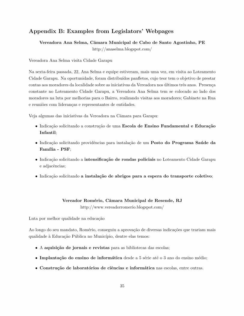
Appendix B: Examples from Legislators’ Webpages

Vereadora Ana Selma, Camara Municipal de Cabo de Santo Agostinho, PE

http://anaselma.blogspot.com/

Vereadora Ana Selma visita Cidade Garapu

Na sexta-feira passada, 22, Ana Selma e equipe estiveram, mais uma vez, em visita ao LoteamentoCidade Garapu. Na oportunidade, foram distribuıdos panfletos, cujo teor tem o objetivo de prestarcontas aos moradores da localidade sobre as iniciativas da Vereadora nos ultimos tres anos. Presencaconstante no Loteamento Cidade Garapu, a Vereadora Ana Selma tem se colocado ao lado dosmoradores na luta por melhorias para o Bairro, realizando visitas aos moradores; Gabinete na Ruae reunioes com liderancas e representantes de entidades.

Veja algumas das iniciativas da Vereadora na Camara para Garapu:

• Indicacao solicitando a construcao de uma Escola de Ensino Fundamental e Educacao

Infantil;

• Indicacao solicitando providencias para instalacao de um Posto do Programa Saude da

Famılia - PSF;

• Indicacao solicitando a intensificacao de rondas policiais no Loteamento Cidade Garapue adjacencias;

• Indicacao solicitando a instalacao de abrigos para a espera do transporte coletivo;

Vereador Romerio, Camara Municipal de Resende, RJ

http://www.vereadorromerio.blogspot.com/

Luta por melhor qualidade na educacao

Ao longo do seu mandato, Romerio, conseguiu a aprovacao de diversas indicacoes que trariam maisqualidade a Educacao Publica no Municıpio, dentre elas temos:

• A aquisicao de jornais e revistas para as bibliotecas das escolas;

• Implantacao do ensino de informatica desde a 5 serie ate o 3 ano do ensino medio;

• Construcao de laboratorios de ciencias e informatica nas escolas, entre outras.

35

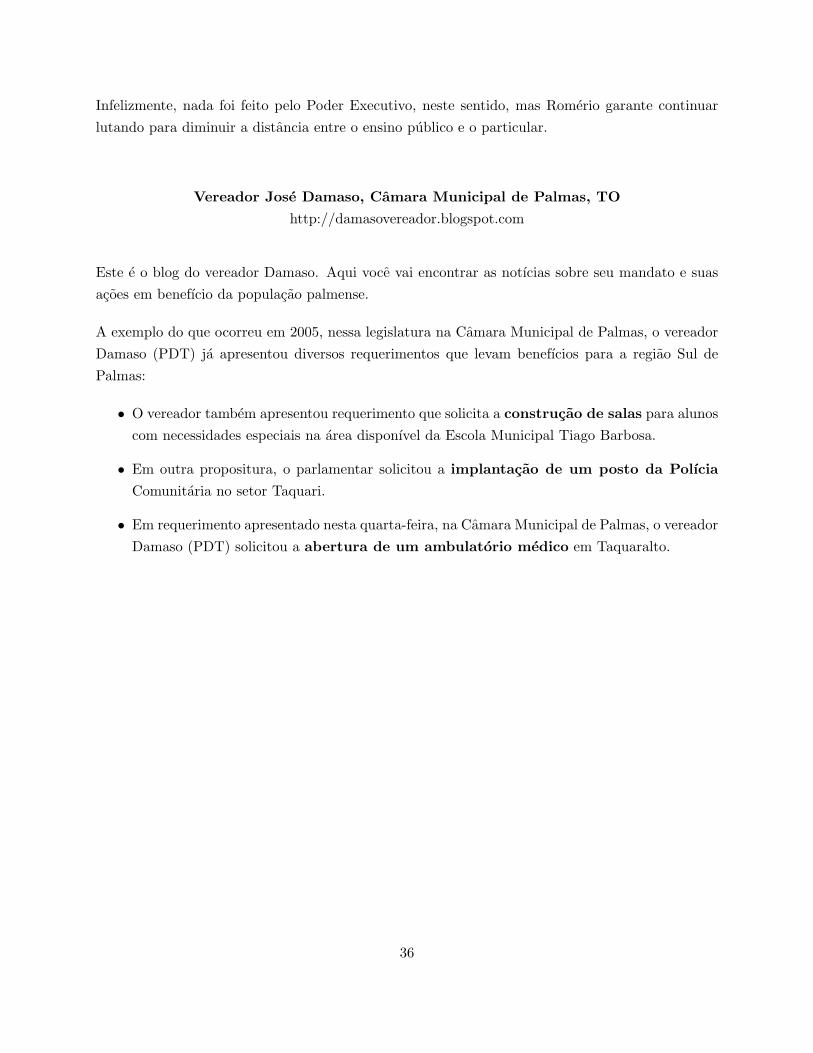
Infelizmente, nada foi feito pelo Poder Executivo, neste sentido, mas Romerio garante continuarlutando para diminuir a distancia entre o ensino publico e o particular.

Vereador Jose Damaso, Camara Municipal de Palmas, TO

http://damasovereador.blogspot.com

Este e o blog do vereador Damaso. Aqui voce vai encontrar as notıcias sobre seu mandato e suasacoes em benefıcio da populacao palmense.

A exemplo do que ocorreu em 2005, nessa legislatura na Camara Municipal de Palmas, o vereadorDamaso (PDT) ja apresentou diversos requerimentos que levam benefıcios para a regiao Sul dePalmas:

• O vereador tambem apresentou requerimento que solicita a construcao de salas para alunoscom necessidades especiais na area disponıvel da Escola Municipal Tiago Barbosa.

• Em outra propositura, o parlamentar solicitou a implantacao de um posto da Polıcia

Comunitaria no setor Taquari.

• Em requerimento apresentado nesta quarta-feira, na Camara Municipal de Palmas, o vereadorDamaso (PDT) solicitou a abertura de um ambulatorio medico em Taquaralto.

36

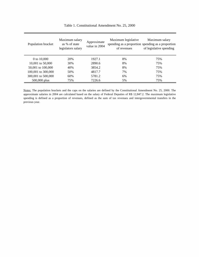
Table 1. Constitutional Amendment No. 25, 2000

0 to 10,000 20% 1927.1 8% 75%10,001 to 50,000 30% 2890.6 8% 75%50,001 to 100,000 40% 3854.2 8% 75%100,001 to 300,000 50% 4817.7 7% 75%300,001 to 500,000 60% 5781.2 6% 75%

500,000 plus 75% 7226.6 5% 75%

Maximum salary spending as a proportion of legislative spending

Population bracketMaximum salary

as % of state legislators salary

Approximate value in 2004

Maximum legislative spending as a proportion

of revenues

Notes: The population brackets and the caps on the salaries are defined by the Constitutional Amendment No. 25, 2000. The approximate salaries in 2004 are calculated based on the salary of Federal Deputies of R$ 12,847.2. The maximum legislative spending is defined as a proportion of revenues, defined as the sum of tax revenues and intergovernmental transfers in the previous year.

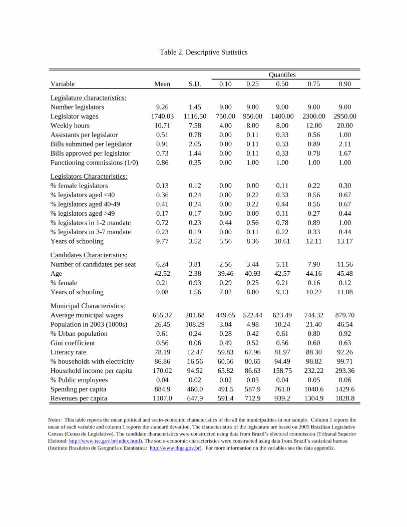
Table 2. Descriptive Statistics

QuantilesVariable Mean S.D. 0.10 0.25 0.50 0.75 0.90

Legislature characteristics:Number legislators 9.26 1.45 9.00 9.00 9.00 9.00 9.00Legislator wages 1740.03 1116.50 750.00 950.00 1400.00 2300.00 2950.00Weekly hours 10.71 7.58 4.00 8.00 8.00 12.00 20.00Assistants per legislator 0.51 0.78 0.00 0.11 0.33 0.56 1.00Bills submitted per legislator 0.91 2.05 0.00 0.11 0.33 0.89 2.11Bills approved per legislator 0.73 1.44 0.00 0.11 0.33 0.78 1.67Functioning commissions (1/0) 0.86 0.35 0.00 1.00 1.00 1.00 1.00

Legislators Characteristics:% female legislators 0.13 0.12 0.00 0.00 0.11 0.22 0.30% legislators aged <40 0.36 0.24 0.00 0.22 0.33 0.56 0.67% legislators aged 40-49 0.41 0.24 0.00 0.22 0.44 0.56 0.67% legislators aged >49 0.17 0.17 0.00 0.00 0.11 0.27 0.44% legislators in 1-2 mandate 0.72 0.23 0.44 0.56 0.78 0.89 1.00% legislators in 3-7 mandate 0.23 0.19 0.00 0.11 0.22 0.33 0.44Years of schooling 9.77 3.52 5.56 8.36 10.61 12.11 13.17

Candidates Characteristics:Number of candidates per seat 6.24 3.81 2.56 3.44 5.11 7.90 11.56Age 42.52 2.38 39.46 40.93 42.57 44.16 45.48% female 0.21 0.93 0.29 0.25 0.21 0.16 0.12Years of schooling 9.08 1.56 7.02 8.00 9.13 10.22 11.08

Municipal Characteristics:Average municipal wages 655.32 201.68 449.65 522.44 623.49 744.32 879.70Population in 2003 (1000s) 26.45 108.29 3.04 4.98 10.24 21.40 46.54% Urban population 0.61 0.24 0.28 0.42 0.61 0.80 0.92Gini coefficient 0.56 0.06 0.49 0.52 0.56 0.60 0.63Literacy rate 78.19 12.47 59.83 67.96 81.97 88.30 92.26% households with electricity 86.86 16.56 60.56 80.65 94.49 98.82 99.71Household income per capita 170.02 94.52 65.82 86.63 158.75 232.22 293.36% Public employees 0.04 0.02 0.02 0.03 0.04 0.05 0.06Spending per capita 884.9 460.0 491.5 587.9 761.0 1040.6 1429.6Revenues per capita 1107.0 647.9 591.4 712.9 939.2 1304.9 1828.8

Notes: This table reports the mean political and socio-economic characteristics of the all the municipalities in our sample. Column 1 reports the mean of each variable and column 1 reports the standard deviation. The characteristics of the legislature are based on 2005 Brazilian Legislative Census (Censo do Legislativo). The candidate characteristics were constructed using data from Brazil’s electoral commission (Tribunal Superior Eleitoral: http://www.tse.gov.br/index.html). The socio-economic characteristics were constructed using data from Brazil’s statistical bureau (Instituto Brasileiro de Geografia e Estatistica: http://www.ibge.gov.br). For more information on the variables see the data appendix.

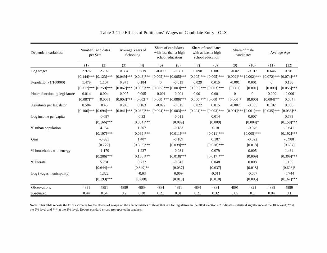
Table 3. The Effects of Politicians’ Wages on Candidate Entry - OLS

(1) (2) (3) (4) (5) (6) (7) (8) (9) (10) (11) (12)Log wages 2.976 2.702 0.834 0.719 -0.099 -0.081 0.098 0.081 -0.02 -0.013 0.646 0.819 [0.144]*** [0.123]*** [0.049]*** [0.043]*** [0.005]*** [0.005]*** [0.005]*** [0.005]*** [0.002]*** [0.002]*** [0.072]*** [0.074]***Population (1/100000) 1.479 1.107 0.375 0.184 0 -0.015 0.029 0.015 -0.001 0.001 0 0.166 [0.317]*** [0.259]*** [0.062]*** [0.033]*** [0.005]*** [0.003]*** [0.005]*** [0.003]*** [0.001] [0.001] [0.000] [0.055]***Hours functioning legislature 0.014 0.004 0.007 0.005 -0.001 -0.001 0.001 0.001 0 0 -0.009 -0.006

[0.007]** [0.006] [0.003]*** [0.002]* [0.000]*** [0.000]*** [0.000]*** [0.000]*** [0.000]* [0.000] [0.004]** [0.004]Assistants per legislator 0.584 0.45 0.245 0.163 -0.022 -0.015 0.022 0.015 -0.007 -0.005 0.102 0.086 [0.106]*** [0.094]*** [0.041]*** [0.032]*** [0.004]*** [0.003]*** [0.004]*** [0.003]*** [0.001]*** [0.001]*** [0.035]*** [0.036]**Log income per capita -0.697 0.33 -0.011 0.014 0.007 0.733 [0.166]*** [0.084]*** [0.009] [0.009] [0.004]* [0.150]***% urban population 4.154 1.507 -0.183 0.18 -0.076 -0.641

[0.197]*** [0.099]*** [0.011]*** [0.011]*** [0.005]*** [0.192]***Gini -0.861 1.407 -0.189 0.187 -0.022 -0.988

[0.722] [0.353]*** [0.039]*** [0.038]*** [0.018] [0.637]% households with energy -1.179 1.237 -0.081 0.079 0.005 1.434

[0.286]*** [0.166]*** [0.018]*** [0.017]*** [0.009] [0.309]***% literate 5.781 0.772 -0.043 0.048 0.008 1.139

[0.644]*** [0.349]** [0.037] [0.037] [0.018] [0.608]*Log (wages municipality) 1.322 -0.03 0.009 -0.011 -0.007 -0.744

[0.193]*** [0.088] [0.010] [0.010] [0.005] [0.167]***

Observations 4891 4891 4889 4889 4891 4891 4891 4891 4891 4891 4889 4889R-squared 0.44 0.54 0.2 0.38 0.21 0.31 0.21 0.32 0.05 0.1 0.04 0.1

Dependent variables: Share of male candidates Average AgeNumber Candidates

per SeatAverage Years of

Schooling

Share of candidates with less than a high

school education

Share of candidates with at least a high school education

Notes: This table reports the OLS estimates for the effects of wages on the characteristics of those that ran for legislature in the 2004 elections. * indicates statistical significance at the 10% level, ** at the 5% level and *** at the 1% level. Robust standard errors are reported in brackets.

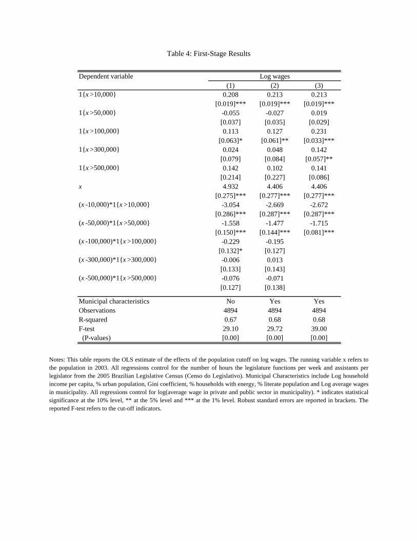
Table 4: First-Stage Results

Dependent variable(1) (2) (3)

1{x >10,000} 0.208 0.213 0.213 [0.019]*** [0.019]*** [0.019]***1{x >50,000} -0.055 -0.027 0.019 [0.037] [0.035] [0.029]1{x >100,000} 0.113 0.127 0.231 [0.063]* [0.061]** [0.033]***1{x >300,000} 0.024 0.048 0.142 [0.079] [0.084] [0.057]**1{x >500,000} 0.142 0.102 0.141

[0.214] [0.227] [0.086]x 4.932 4.406 4.406 [0.275]*** [0.277]*** [0.277]***(x -10,000)*1{x >10,000} -3.054 -2.669 -2.672 [0.286]*** [0.287]*** [0.287]***(x -50,000)*1{x >50,000} -1.558 -1.477 -1.715 [0.150]*** [0.144]*** [0.081]***(x -100,000)*1{x >100,000} -0.229 -0.195 [0.132]* [0.127](x -300,000)*1{x >300,000} -0.006 0.013 [0.133] [0.143](x -500,000)*1{x >500,000} -0.076 -0.071 [0.127] [0.138]

Municipal characteristics No Yes YesObservations 4894 4894 4894R-squared 0.67 0.68 0.68F-test 29.10 29.72 39.00 (P-values) [0.00] [0.00] [0.00]

Log wages

Notes: This table reports the OLS estimate of the effects of the population cutoff on log wages. The running variable x refers to the population in 2003. All regressions control for the number of hours the legislature functions per week and assistants per legislator from the 2005 Brazilian Legislative Census (Censo do Legislativo). Municipal Characteristics include Log household income per capita, % urban population, Gini coefficient, % households with energy, % literate population and Log average wages in municipality. All regressions control for log(average wage in private and public sector in municipality). * indicates statistical significance at the 10% level, ** at the 5% level and *** at the 1% level. Robust standard errors are reported in brackets. The reported F-test refers to the cut-off indicators.

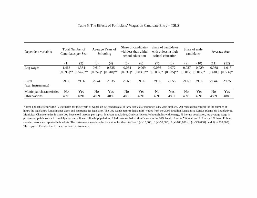
Table 5. The Effects of Politicians’ Wages on Candidate Entry – TSLS

 

Dependent variable:

(1) (2) (3) (4) (5) (6) (7) (8) (9) (10) (11) (12)Log wages 1.463 1.334 0.619 0.625 -0.064 -0.069 0.066 0.072 -0.027 -0.029 -0.988 -1.015

[0.598]** [0.547]** [0.352]* [0.318]** [0.037]* [0.035]** [0.037]* [0.035]** [0.017] [0.017]* [0.601] [0.586]*

F-test 29.66 29.56 29.44 29.35 29.66 29.56 29.66 29.56 29.66 29.56 29.44 29.35(exc. instruments)

Municipal characteristics No Yes No Yes No Yes No Yes No Yes No YesObservations 4891 4891 4889 4889 4891 4891 4891 4891 4891 4891 4889 4889

Total Number of Candidates per Seat

Average Years of Schooling

Share of candidates with less than a high

school education

Share of candidates with at least a high school education

Share of male candidates Average Age

Notes: The table reports the IV estimates for the effects of wages on the characteristics of those that ran for legislature in the 2004 elections. All regressions control for the number of hours the legislature functions per week and assistants per legislator. The Log wages refer to legislators' wages from the 2005 Brazilian Legislative Census (Censo do Legislativo). Municipal Characteristics include Log household income per capita, % urban population, Gini coefficient, % households with energy, % literate population, log average wage in private and public sector in municipality, and a linear spline in population. * indicates statistical significance at the 10% level, ** at the 5% level and *** at the 1% level. Robust standard errors are reported in brackets. The instruments used are the indicators for the cutoffs at 1{x>10,000}, 1{x>50,000}, 1{x>100,000}, 1{x>300,000} and 1{x>500,000}. The reported F-test refers to these excluded instruments.

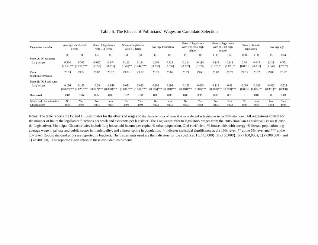
Table 6. The Effects of Politicians’ Wages on Candidate Selection

Dependent variable:

(1) (2) (3) (4) (5) (6) (7) (8) (9) (10) (11) (12) (13) (14) (15) (16)Panel A: IV estimates

Log Wages 0.364 0.395 -0.067 -0.074 0.113 0.124 1.009 0.913 -0.114 -0.114 0.145 0.141 0.04 0.045 1.011 0.551[0.153]** [0.150]*** [0.057] [0.056] [0.045]** [0.044]*** [0.857] [0.836] [0.077] [0.074] [0.076]* [0.073]* [0.031] [0.031] [2.847] [2.787]

F-test 29.83 29.72 29.83 29.72 29.83 29.72 29.79 29.65 29.79 29.65 29.83 29.72 29.83 29.72 29.83 29.72(excl. instruments)

Panel B: OLS estimatesLog Wages 0.176 0.185 -0.05 -0.049 0.051 0.053 0.805 0.696 -0.123 -0.093 0.113 0.09 -0.004 -0.009 -0.892 -0.521

[0.022]*** [0.025]*** [0.007]*** [0.008]*** [0.006]*** [0.007]*** [0.116]*** [0.118]*** [0.010]*** [0.009]*** [0.010]*** [0.010]*** [0.003] [0.004]** [0.381]** [0.398]

R-squared 0.02 0.06 0.02 0.06 0.02 0.08 0.03 0.06 0.09 0.19 0.06 0.13 0 0.02 0 0.03

Municipal characteristics No Yes No Yes No Yes No Yes No Yes No Yes No Yes No YesObservations 4894 4894 4894 4894 4894 4894 4893 4893 4893 4893 4893 4893 4894 4894 4894 4894

Average Number of Terms

Share of legislators with 1-2 terms

Share of legislators with 3-7 terms Average Education

Share of legislators with less than high

school

Share of legislators with at least high

school

Share of female legislators Average age

Notes: The table reports the IV and OLS estimates for the effects of wages on the characteristics of those that were elected as legislators in the 2004 elections. All regressions control for the number of hours the legislature functions per week and assistants per legislator. The Log wages refer to legislators' wages from the 2005 Brazilian Legislative Census (Censo do Legislativo). Municipal Characteristics include Log household income per capita, % urban population, Gini coefficient, % households with energy, % literate population, log average wage in private and public sector in municipality, and a linear spline in population. * indicates statistical significance at the 10% level, ** at the 5% level and *** at the 1% level. Robust standard errors are reported in brackets. The instruments used are the indicators for the cutoffs at 1{x>10,000}, 1{x>50,000}, 1{x>100,000}, 1{x>300,000} and 1{x>500,000}. The reported F-test refers to these excluded instruments.

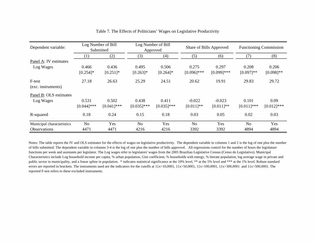
Table 7. The Effects of Politicians’ Wages on Legislative Productivity

(1) (2) (3) (4) (5) (6) (7) (8)Panel A: IV estimates

Log Wages 0.466 0.436 0.495 0.506 0.275 0.297 0.208 0.206[0.254]* [0.251]* [0.263]* [0.264]* [0.096]*** [0.099]*** [0.097]** [0.098]**

F-test 27.18 26.63 25.29 24.51 20.62 19.91 29.83 29.72(exc. instruments)

Panel B: OLS estimatesLog Wages 0.531 0.502 0.438 0.411 -0.022 -0.023 0.101 0.09

[0.044]*** [0.041]*** [0.035]*** [0.035]*** [0.011]** [0.011]** [0.011]*** [0.012]***

R-squared 0.18 0.24 0.15 0.18 0.03 0.05 0.02 0.03

Municipal characteristics No Yes No Yes No Yes No YesObservations 4471 4471 4216 4216 3392 3392 4894 4894

Dependent variable: Log Number of Bill Submitted

Log Number of Bill Approved Share of Bills Approved Functioning Commission

Notes: The table reports the IV and OLS estimates for the effects of wages on legislative productivity. The dependent variable in columns 1 and 2 is the log of one plus the number of bills submitted. The dependent variable in columns 3-4 is the log of one plus the number of bills approved. All regressions control for the number of hours the legislature functions per week and assistants per legislator. The Log wages refer to legislators' wages from the 2005 Brazilian Legislative Census (Censo do Legislativo). Municipal Characteristics include Log household income per capita, % urban population, Gini coefficient, % households with energy, % literate population, log average wage in private and public sector in municipality, and a linear spline in population. * indicates statistical significance at the 10% level, ** at the 5% level and *** at the 1% level. Robust standard errors are reported in brackets. The instruments used are the indicators for the cutoffs at 1{x>10,000}, 1{x>50,000}, 1{x>100,000}, 1{x>300,000} and 1{x>500,000}. The reported F-test refers to these excluded instruments.

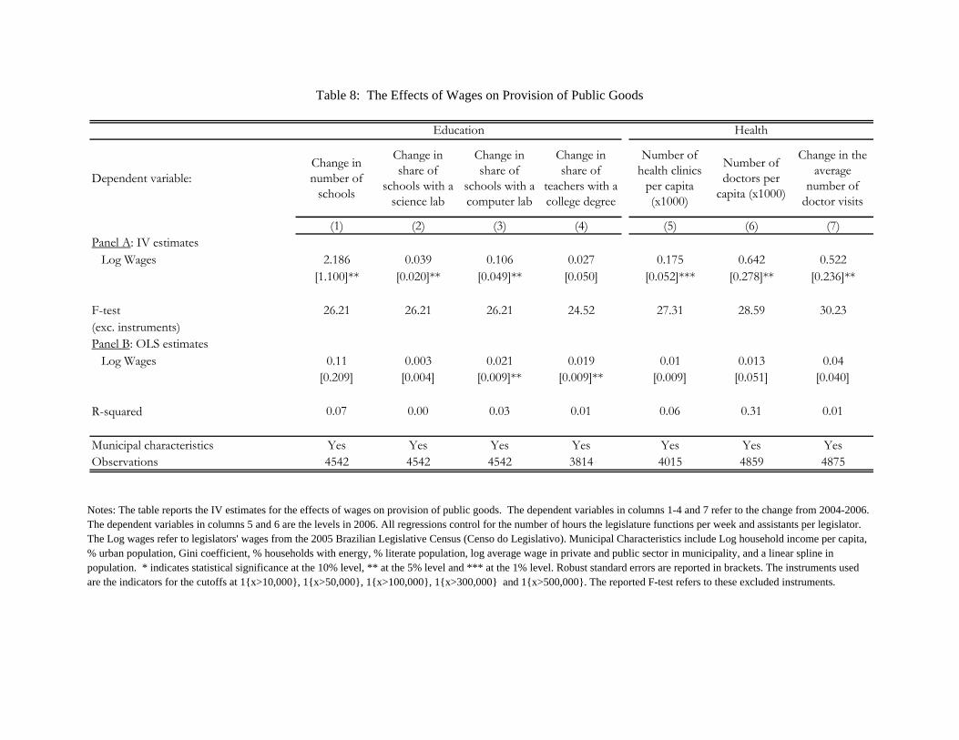
Table 8: The Effects of Wages on Provision of Public Goods

Dependent variable:Change in number of

schools

Change in share of

schools with a science lab

Change in share of

schools with a computer lab

Change in share of

teachers with a college degree

Number of health clinics

per capita (x1000)

Number of doctors per

capita (x1000)

Change in the average

number of doctor visits

(1) (2) (3) (4) (5) (6) (7)Panel A: IV estimates

Log Wages 2.186 0.039 0.106 0.027 0.175 0.642 0.522[1.100]** [0.020]** [0.049]** [0.050] [0.052]*** [0.278]** [0.236]**

F-test 26.21 26.21 26.21 24.52 27.31 28.59 30.23(exc. instruments)Panel B: OLS estimates

Log Wages 0.11 0.003 0.021 0.019 0.01 0.013 0.04[0.209] [0.004] [0.009]** [0.009]** [0.009] [0.051] [0.040]

R-squared 0.07 0.00 0.03 0.01 0.06 0.31 0.01

Municipal characteristics Yes Yes Yes Yes Yes Yes YesObservations 4542 4542 4542 3814 4015 4859 4875

Education Health

Notes: The table reports the IV estimates for the effects of wages on provision of public goods. The dependent variables in columns 1-4 and 7 refer to the change from 2004-2006. The dependent variables in columns 5 and 6 are the levels in 2006. All regressions control for the number of hours the legislature functions per week and assistants per legislator. The Log wages refer to legislators' wages from the 2005 Brazilian Legislative Census (Censo do Legislativo). Municipal Characteristics include Log household income per capita, % urban population, Gini coefficient, % households with energy, % literate population, log average wage in private and public sector in municipality, and a linear spline in population. * indicates statistical significance at the 10% level, ** at the 5% level and *** at the 1% level. Robust standard errors are reported in brackets. The instruments used are the indicators for the cutoffs at 1{x>10,000}, 1{x>50,000}, 1{x>100,000}, 1{x>300,000} and 1{x>500,000}. The reported F-test refers to these excluded instruments.

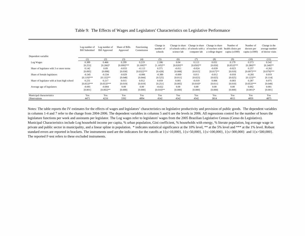
Table 9: The Effects of Wages and Legislators' Characteristics on Legislative Performance

Dependent variable:

Log number of Bill Submitted

Log number of Bill Approved

Share of Bills Approved

Functioning Commission

Change in number of

schools

Change in share of schools with a

science lab

Change in share of schools with a

computer lab

Change in share of teachers with a college degree

Number of health clinics per capita (x1000)

Number of doctors per

capita (x1000)

Change in the average number of doctor visits

(1) (2) (3) (4) (5) (6) (7) (8) (9) (10) (11)Log Wages 0.389 0.466 0.299 0.219 2.186 0.04 0.113 0.031 0.179 0.573 0.542

[0.253] [0.266]* [0.099]*** [0.100]** [1.105]** [0.020]** [0.050]** [0.050] [0.053]*** [0.280]** [0.240]**Share of legislator with 3 or more terms 0.142 0.09 -0.033 -0.113 0.571 -0.011 -0.024 -0.039 -0.023 0.257 -0.262

[0.095] [0.098] [0.030] [0.032]*** [0.428] [0.008] [0.015] [0.017]** [0.019] [0.097]*** [0.079]***Share of female legislators -0.345 -0.334 -0.029 -0.006 -0.389 -0.009 0.011 -0.012 -0.018 -0.281 0.019

[0.119]*** [0.132]** [0.048] [0.044] [0.525] [0.011] [0.023] [0.025] [0.025] [0.123]** [0.114]Share of legislator with at least high school 0.231 0.217 0.015 0.012 0.059 0.001 -0.019 0.006 -0.003 0.287 0.075

[0.053]*** [0.053]*** [0.019] [0.019] [0.251] [0.005] [0.010]* [0.011] [0.010] [0.053]*** [0.049]Average age of legislators -0.001 -0.004 0.00 0.00 -0.022 0.00 0.00 0.00 0.00 0.002 0.001

[0.001] [0.002]** [0.000] [0.000] [0.010]** [0.000] [0.000] [0.000] [0.000] [0.001]* [0.001]

Municipal characteristics Yes Yes Yes Yes Yes Yes Yes Yes Yes Yes YesObservations 4471 4216 3392 4894 4542 4542 4542 3814 4015 4859 4875

Notes: The table reports the IV estimates for the effects of wages and legislators’ characteristics on legislative productivity and provision of public goods. The dependent variables in columns 1-4 and 7 refer to the change from 2004-2006. The dependent variables in columns 5 and 6 are the levels in 2006. All regressions control for the number of hours the legislature functions per week and assistants per legislator. The Log wages refer to legislators' wages from the 2005 Brazilian Legislative Census (Censo do Legislativo). Municipal Characteristics include Log household income per capita, % urban population, Gini coefficient, % households with energy, % literate population, log average wage in private and public sector in municipality, and a linear spline in population. * indicates statistical significance at the 10% level, ** at the 5% level and *** at the 1% level. Robust standard errors are reported in brackets. The instruments used are the indicators for the cutoffs at 1{x>10,000}, 1{x>50,000}, 1{x>100,000}, 1{x>300,000} and 1{x>500,000}. The reported F-test refers to these excluded instruments.

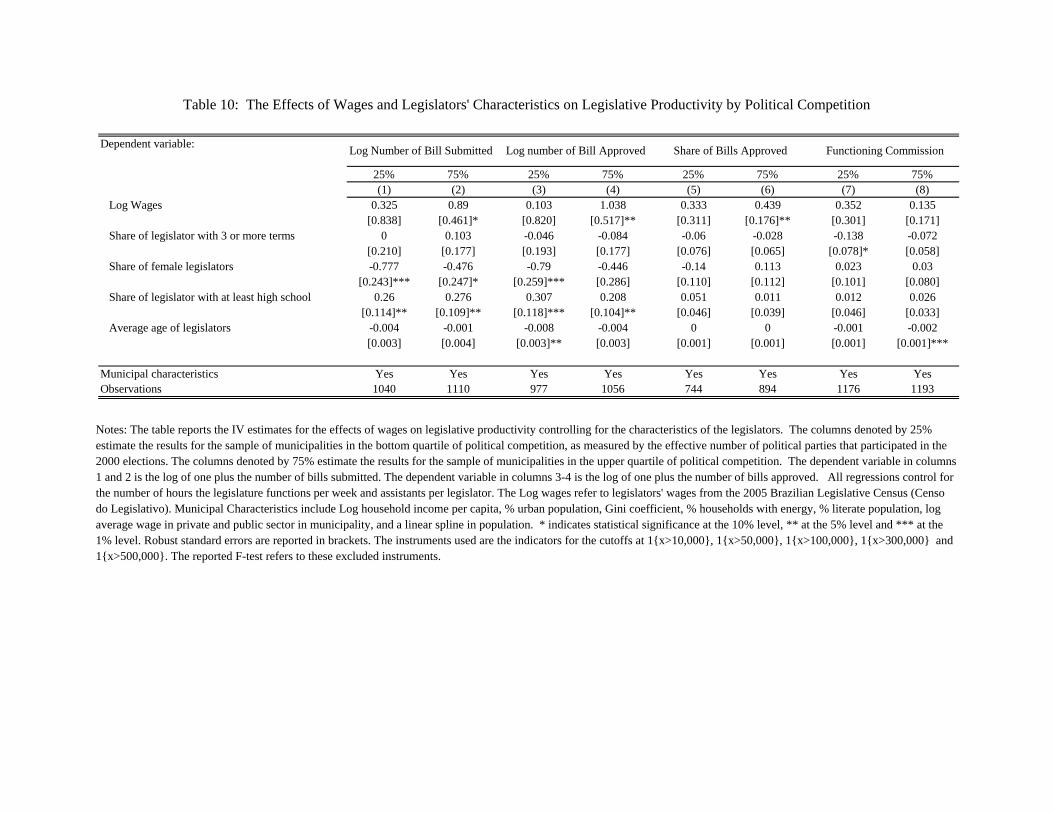
Table 10: The Effects of Wages and Legislators' Characteristics on Legislative Productivity by Political Competition

Dependent variable:

25% 75% 25% 75% 25% 75% 25% 75%(1) (2) (3) (4) (5) (6) (7) (8)

Log Wages 0.325 0.89 0.103 1.038 0.333 0.439 0.352 0.135[0.838] [0.461]* [0.820] [0.517]** [0.311] [0.176]** [0.301] [0.171]

Share of legislator with 3 or more terms 0 0.103 -0.046 -0.084 -0.06 -0.028 -0.138 -0.072[0.210] [0.177] [0.193] [0.177] [0.076] [0.065] [0.078]* [0.058]

Share of female legislators -0.777 -0.476 -0.79 -0.446 -0.14 0.113 0.023 0.03[0.243]*** [0.247]* [0.259]*** [0.286] [0.110] [0.112] [0.101] [0.080]

Share of legislator with at least high school 0.26 0.276 0.307 0.208 0.051 0.011 0.012 0.026[0.114]** [0.109]** [0.118]*** [0.104]** [0.046] [0.039] [0.046] [0.033]

Average age of legislators -0.004 -0.001 -0.008 -0.004 0 0 -0.001 -0.002[0.003] [0.004] [0.003]** [0.003] [0.001] [0.001] [0.001] [0.001]***

Municipal characteristics Yes Yes Yes Yes Yes Yes Yes YesObservations 1040 1110 977 1056 744 894 1176 1193

Log Number of Bill Submitted Log number of Bill Approved Share of Bills Approved Functioning Commission

Notes: The table reports the IV estimates for the effects of wages on legislative productivity controlling for the characteristics of the legislators. The columns denoted by 25% estimate the results for the sample of municipalities in the bottom quartile of political competition, as measured by the effective number of political parties that participated in the 2000 elections. The columns denoted by 75% estimate the results for the sample of municipalities in the upper quartile of political competition. The dependent variable in columns 1 and 2 is the log of one plus the number of bills submitted. The dependent variable in columns 3-4 is the log of one plus the number of bills approved. All regressions control for the number of hours the legislature functions per week and assistants per legislator. The Log wages refer to legislators' wages from the 2005 Brazilian Legislative Census (Censo do Legislativo). Municipal Characteristics include Log household income per capita, % urban population, Gini coefficient, % households with energy, % literate population, log average wage in private and public sector in municipality, and a linear spline in population. * indicates statistical significance at the 10% level, ** at the 5% level and *** at the 1% level. Robust standard errors are reported in brackets. The instruments used are the indicators for the cutoffs at 1{x>10,000}, 1{x>50,000}, 1{x>100,000}, 1{x>300,000} and 1{x>500,000}. The reported F-test refers to these excluded instruments.

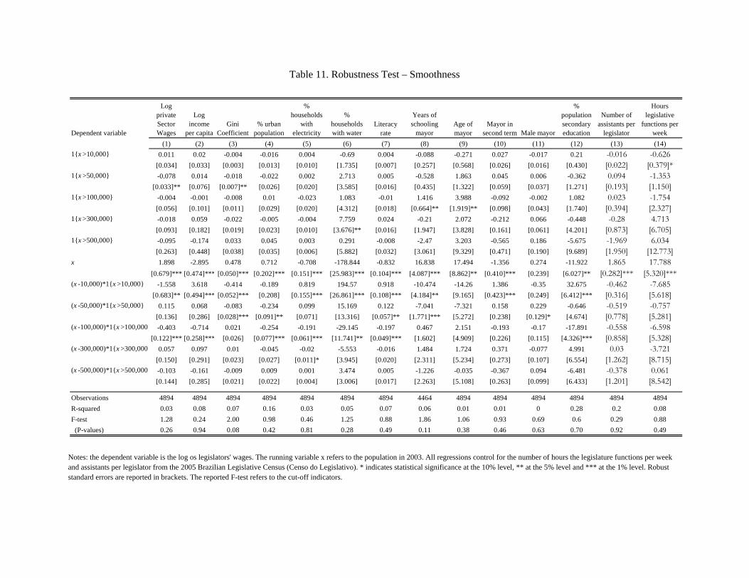
(1) (2) (3) (4) (5) (6) (7) (8) (9) (10) (11) (12) (13) (14)1{x >10,000} 0.011 0.02 -0.004 -0.016 0.004 -0.69 0.004 -0.088 -0.271 0.027 -0.017 0.21 -0.016 -0.626 [0.034] [0.033] [0.003] [0.013] [0.010] [1.735] [0.007] [0.257] [0.568] [0.026] [0.016] [0.430] [0.022] [0.379]*1{x >50,000} -0.078 0.014 -0.018 -0.022 0.002 2.713 0.005 -0.528 1.863 0.045 0.006 -0.362 0.094 -1.353 [0.033]** [0.076] [0.007]** [0.026] [0.020] [3.585] [0.016] [0.435] [1.322] [0.059] [0.037] [1.271] [0.193] [1.150]1{x >100,000} -0.004 -0.001 -0.008 0.01 -0.023 1.083 -0.01 1.416 3.988 -0.092 -0.002 1.082 0.023 -1.754 [0.056] [0.101] [0.011] [0.029] [0.020] [4.312] [0.018] [0.664]** [1.919]** [0.098] [0.043] [1.740] [0.394] [2.327]1{x >300,000} -0.018 0.059 -0.022 -0.005 -0.004 7.759 0.024 -0.21 2.072 -0.212 0.066 -0.448 -0.28 4.713 [0.093] [0.182] [0.019] [0.023] [0.010] [3.676]** [0.016] [1.947] [3.828] [0.161] [0.061] [4.201] [0.873] [6.705]1{x >500,000} -0.095 -0.174 0.033 0.045 0.003 0.291 -0.008 -2.47 3.203 -0.565 0.186 -5.675 -1.969 6.034

[0.263] [0.448] [0.038] [0.035] [0.006] [5.882] [0.032] [3.061] [9.329] [0.471] [0.190] [9.689] [1.950] [12.773]x 1.898 -2.895 0.478 0.712 -0.708 -178.844 -0.832 16.838 17.494 -1.356 0.274 -11.922 1.865 17.788 [0.679]*** [0.474]*** [0.050]*** [0.202]*** [0.151]*** [25.983]*** [0.104]*** [4.087]*** [8.862]** [0.410]*** [0.239] [6.027]** [0.282]*** [5.320]***(x -10,000)*1{x >10,000} -1.558 3.618 -0.414 -0.189 0.819 194.57 0.918 -10.474 -14.26 1.386 -0.35 32.675 -0.462 -7.685 [0.683]** [0.494]*** [0.052]*** [0.208] [0.155]*** [26.861]*** [0.108]*** [4.184]** [9.165] [0.423]*** [0.249] [6.412]*** [0.316] [5.618](x -50,000)*1{x >50,000} 0.115 0.068 -0.083 -0.234 0.099 15.169 0.122 -7.041 -7.321 0.158 0.229 -0.646 -0.519 -0.757 [0.136] [0.286] [0.028]*** [0.091]** [0.071] [13.316] [0.057]** [1.771]*** [5.272] [0.238] [0.129]* [4.674] [0.778] [5.281](x -100,000)*1{x >100,000} -0.403 -0.714 0.021 -0.254 -0.191 -29.145 -0.197 0.467 2.151 -0.193 -0.17 -17.891 -0.558 -6.598 [0.122]*** [0.258]*** [0.026] [0.077]*** [0.061]*** [11.741]** [0.049]*** [1.602] [4.909] [0.226] [0.115] [4.326]*** [0.858] [5.328](x -300,000)*1{x >300,000} 0.057 0.097 0.01 -0.045 -0.02 -5.553 -0.016 1.484 1.724 0.371 -0.077 4.991 0.03 -3.721 [0.150] [0.291] [0.023] [0.027] [0.011]* [3.945] [0.020] [2.311] [5.234] [0.273] [0.107] [6.554] [1.262] [8.715](x -500,000)*1{x >500,000} -0.103 -0.161 -0.009 0.009 0.001 3.474 0.005 -1.226 -0.035 -0.367 0.094 -6.481 -0.378 0.061 [0.144] [0.285] [0.021] [0.022] [0.004] [3.006] [0.017] [2.263] [5.108] [0.263] [0.099] [6.433] [1.201] [8.542]

Observations 4894 4894 4894 4894 4894 4894 4894 4464 4894 4894 4894 4894 4894 4894R-squared 0.03 0.08 0.07 0.16 0.03 0.05 0.07 0.06 0.01 0.01 0 0.28 0.2 0.08F-test 1.28 0.24 2.00 0.98 0.46 1.25 0.88 1.86 1.06 0.93 0.69 0.6 0.29 0.88 (P-values) 0.26 0.94 0.08 0.42 0.81 0.28 0.49 0.11 0.38 0.46 0.63 0.70 0.92 0.49

Dependent variableLiteracy

rate

% population secondary education

Age of mayor

Mayor in second term

Number of assistants per

legislator

Hours legislative

functions per week

Log private Sector Wages

Log income

per capitaGini

Coefficient% urban

population

% households

with electricity

% households with water

Years of schooling

mayor Male mayor

Notes: the dependent variable is the log os legislators' wages. The running variable x refers to the population in 2003. All regressions control for the number of hours the legislature functions per week and assistants per legislator from the 2005 Brazilian Legislative Census (Censo do Legislativo). * indicates statistical significance at the 10% level, ** at the 5% level and *** at the 1% level. Robust standard errors are reported in brackets. The reported F-test refers to the cut-off indicators.

Table 11. Robustness Test – Smoothness

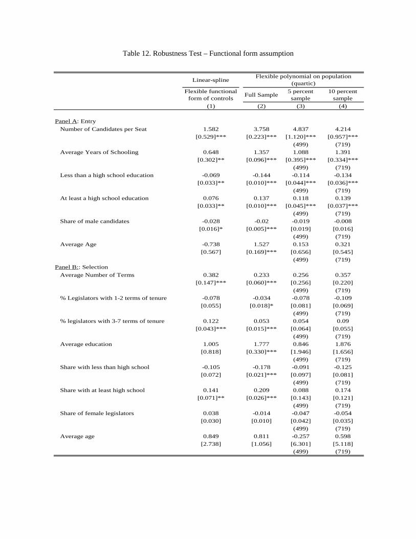
Table 12. Robustness Test – Functional form assumption

Linear-spline

Flexible functional form of controls Full Sample 5 percent

sample10 percent

sample(1) (2) (3) (4)

Panel A: EntryNumber of Candidates per Seat 1.582 3.758 4.837 4.214

[0.529]*** [0.223]*** [1.120]*** [0.957]***(499) (719)

Average Years of Schooling 0.648 1.357 1.088 1.391[0.302]** [0.096]*** [0.395]*** [0.334]***

(499) (719)Less than a high school education -0.069 -0.144 -0.114 -0.134

[0.033]** [0.010]*** [0.044]*** [0.036]***(499) (719)

At least a high school education 0.076 0.137 0.118 0.139[0.033]** [0.010]*** [0.045]*** [0.037]***

(499) (719)Share of male candidates -0.028 -0.02 -0.019 -0.008

[0.016]* [0.005]*** [0.019] [0.016](499) (719)

Average Age -0.738 1.527 0.153 0.321[0.567] [0.169]*** [0.656] [0.545]

(499) (719)Panel B:: Selection

Average Number of Terms 0.382 0.233 0.256 0.357[0.147]*** [0.060]*** [0.256] [0.220]

(499) (719)% Legislators with 1-2 terms of tenure -0.078 -0.034 -0.078 -0.109

[0.055] [0.018]* [0.081] [0.069](499) (719)

% legislators with 3-7 terms of tenure 0.122 0.053 0.054 0.09[0.043]*** [0.015]*** [0.064] [0.055]

(499) (719)Average education 1.005 1.777 0.846 1.876

[0.818] [0.330]*** [1.946] [1.656](499) (719)

Share with less than high school -0.105 -0.178 -0.091 -0.125[0.072] [0.021]*** [0.097] [0.081]

(499) (719)Share with at least high school 0.141 0.209 0.088 0.174

[0.071]** [0.026]*** [0.143] [0.121](499) (719)

Share of female legislators 0.038 -0.014 -0.047 -0.054[0.030] [0.010] [0.042] [0.035]

(499) (719)Average age 0.849 0.811 -0.257 0.598

[2.738] [1.056] [6.301] [5.118](499) (719)

Flexible polynomial on population (quartic)

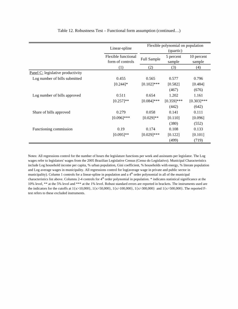
Table 12. Robustness Test – Functional form assumption (continued…)

Linear-spline

Flexible functional form of controls Full Sample 5 percent

sample10 percent

sample(1) (2) (3) (4)

Panel C: legislative productivityLog number of bills submitted 0.455 0.565 0.577 0.796

[0.244]* [0.102]*** [0.582] [0.484](467) (676)

Log number of bills approved 0.511 0.654 1.202 1.161[0.257]** [0.084]*** [0.359]*** [0.303]***

(442) (642)Share of bills approved 0.279 0.058 0.141 0.111

[0.096]*** [0.029]** [0.110] [0.096](380) (552)

Functioning commission 0.19 0.174 0.108 0.133[0.095]** [0.029]*** [0.122] [0.101]

(499) (719)

Flexible polynomial on population (quartic)

Notes: All regressions control for the number of hours the legislature functions per week and assistants per legislator. The Log wages refer to legislators' wages from the 2005 Brazilian Legislative Census (Censo do Legislativo). Municipal Characteristics include Log household income per capita, % urban population, Gini coefficient, % households with energy, % literate population and Log average wages in municipality. All regressions control for log(average wage in private and public sector in municipality). Column 1 controls for a linear-spline in population and a 4th order polynomial in all of the municipal characteristics list above. Columns 2-4 controls for 4th order polynomial in population. * indicates statistical significance at the 10% level, ** at the 5% level and *** at the 1% level. Robust standard errors are reported in brackets. The instruments used are the indicators for the cutoffs at 1{x>10,000}, 1{x>50,000}, 1{x>100,000}, 1{x>300,000} and 1{x>500,000}. The reported F-test refers to these excluded instruments.

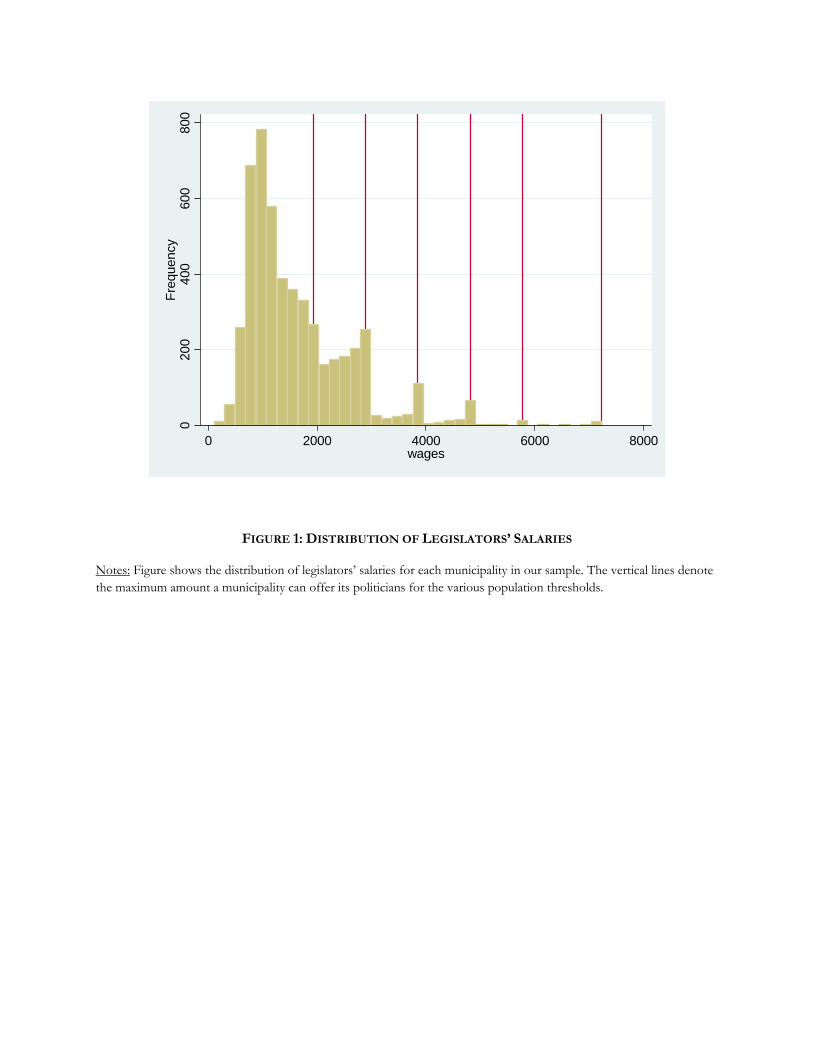
020

040

060

080

0Fr

eque

ncy

0 2000 4000 6000 8000wages

FIGURE 1: DISTRIBUTION OF LEGISLATORS’ SALARIES

Notes: Figure shows the distribution of legislators’ salaries for each municipality in our sample. The vertical lines denote the maximum amount a municipality can offer its politicians for the various population thresholds.

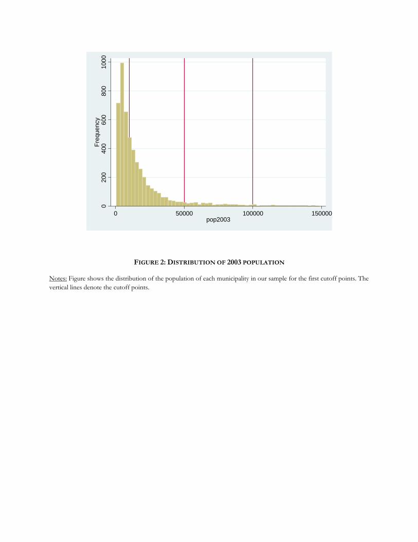
020

040

060

080

010

00Fr

eque

ncy

0 50000 100000 150000pop2003

FIGURE 2: DISTRIBUTION OF 2003 POPULATION

Notes: Figure shows the distribution of the population of each municipality in our sample for the first cutoff points. The vertical lines denote the cutoff points.

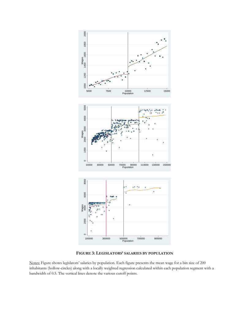
1000

1200

1400

1600

1800

2000

Wag

es

5000 7500 10000 12500 15000Population

010

0020

0030

0040

0050

00W

ages

10000 30000 50000 70000 90000 110000 130000 150000Population

020

0040

0060

0080

00W

ages

100000 300000 500000 700000 900000Population

FIGURE 3: LEGISLATORS’ SALARIES BY POPULATION

Notes: Figure shows legislators’ salaries by population. Each figure presents the mean wage for a bin size of 200 inhabitants (hollow-circles) along with a locally weighted regression calculated within each population segment with a bandwidth of 0.5. The vertical lines denote the various cutoff points.

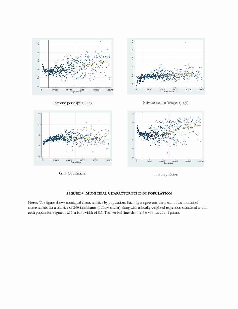
Income per capita (log)

Private Sector Wages (logs)

Gini Coefficient

Literacy Rates

44.

55

5.5

66.

5

0 20000 40000 60000 80000 100000Population

66.

57

7.5

88.

5

0 20000 40000 60000 80000 100000Population

.4.5

.6.7

.8

0 20000 40000 60000 80000 100000Population

.5.6

.7.8

.91

0 20000 40000 60000 80000 100000Population

FIGURE 4: MUNICIPAL CHARACTERISTICS BY POPULATION

Notes: The figure shows municipal characteristics by population. Each figure presents the mean of the municipal characteristic for a bin size of 200 inhabitants (hollow-circles) along with a locally weighted regression calculated within each population segment with a bandwidth of 0.5. The vertical lines denote the various cutoff points.