motor control - project research cit

8/10/2019 Motor Control - Project Research CIT

http://slidepdf.com/reader/full/motor-control-project-research-cit 1/28

DC MOTOR CONTROL



Table of Contents

1. Abstract ...................................................................................................................................................1

2. Objectives ...............................................................................................................................................2

3.

Introduction .............................................................................................................................................3

3.1. DC Machine Features .....................................................................................................................3

3.2. Mathematical Description ..............................................................................................................4

3.3. The DR300 DC Motor by Amira ....................................................................................................7

4. Materials & Methods ............................................................................................................................10

4.1. Calibration Curve .........................................................................................................................10

4.2. System Modelling ........................................................................................................................11

4.3. System Modelling Validation .......................................................................................................13

5. Results & Discussion ............................................................................................................................15

5.1. System Permanence .....................................................................................................................15

5.2. Control Design .............................................................................................................................16

5.3. Model and controller improvement ..............................................................................................17

5.4. Integral Absolute Error (IAE) ......................................................................................................20

6. Conclusion ............................................................................................................................................22

7. References .............................................................................................................................................23

Appendix .......................................................................................................................................................24



1

1.

Abstract

DC motors have many advantages in relation to other machines. The high torque and

simple speed control are good conditions for many applications. For this reason, the study of

controllability of DC motors is very important for the control engineer.

The electrical scheme is studied in order to figure out a model for the rig. The linearity of

the system was studied to analyze its controllability. Some experimental models were figured

out and continuously improved as new speed controllers were designed. Eventually, the

quality of the model was assessed using integral absolute error.

Keywords: DC motor; control; root locus; amira 300; PI controller.



2

2. Objectives

This project aims to analyze the features, implement a model and a controller for the

DR300 DC Motor produced by Amira. Some experiments must to be carried out for

analyzing the machine features in order to understand its operation. A model is to be

evaluated based on technical data from datasheet and experimentally using external control.

Finally, a speed controller must be implemented for controlling the machine with PC -Motor

interface using the software Simulink.



3

3. Introduction

3.1.

DC Machine Features

DC machines can be used as a motor as well as a generator. Currently, the

development of Drive Engineering with alternating current (AC) and economic viability have

favored the replacement of DC motors (DC) by induction motors driven by frequency

inverters. Nevertheless, due to its characteristics and advantages, the DC motor still shows

the best choice in many applications, such as:

Paper Machines

Winders and Unwinders

Laminator

Printing Machinery Extruders

Presser

Lift

Charge Handling and Lifting

by Roller Mills

Rubber Industry

Many industrial processes need to operate with variable speeds. It is possible to

engage gears or friction systems. However these solutions imply the process stalling to make

the change besides a low yield operation. Among the types of engines, the DC motor was the

first to be used in industry and stands out for simplicity in speed control and big torque. The

DC motor is divided into two distinct parts: a fixed (stator or field) and the other movable

(rotor or armature).

The Stator is the fixed part, has pole pieces formed by silicon steel blades juxtaposed.

There is a wire winding the pole pieces forming coils. The Rotor is the moving part of the

motor connected to the drive shaft. The rotor has a silicon steel lamination stack with grooves

where the rotor coils lies. These coils terminals are electrically connected to the collector.



4

Figure 1 – Stator and Rotor

The collector or commutator electrically connects the rotor coils through carbon

brushes to power source in order to allow rotor movement without causing short circuits.

Figure 2 – Collector

The Brushes are made of carbon graphite or carbon. The brushes conduct current from

external source to the collector contacts and the rotor coils. Due to continuous friction, the

brushes require periodic maintenance by replacing the pair of brushes.

Figure 3 - DC Motor and its Brushes

The initial condition for a DC Motor operation is the stator magnetic flux production.

This magnetic flux is obtained by applying direct current in the stator coils. Hence, it the

magnetic poles come up, which become electromagnets with fixed polarity poles. A direct

current from an external source flows through the brushes, commutator and rotor coils, thus

creating magnetic poles on the rotor. The rotor poles are attracted by the stator poles resulting

in a magnetic force. It is mounted over bearings that allow it to spin. Due to magnetic forces

between stator and rotor, the rotor seeks a new equilibrium condition hence moves angularly.

As the rotor coils are powered electrically through the collector and brushes, after

displacement the other coils are fed thus producing magnetic forces again.

3.2. Mathematical Description

The electrical circuit of a motor can be represented by the figure below .



5

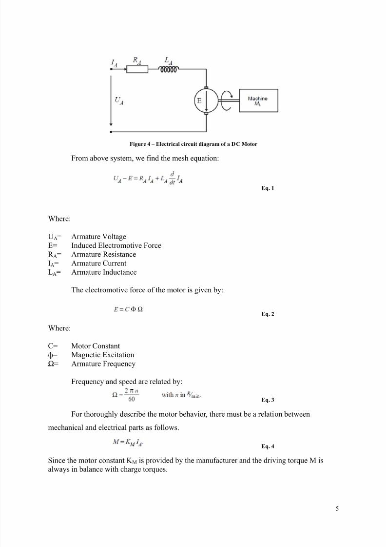
Figure 4 – Electrical circuit diagram of a DC Motor

From above system, we find the mesh equation:

Eq. 1

Where:

UA= Armature Voltage

E= Induced Electromotive Force

R A= Armature Resistance

IA= Armature Current

LA= Armature Inductance

The electromotive force of the motor is given by:

Eq. 2

Where:

C= Motor Constant

ф= Magnetic Excitation

Ω= Armature Frequency

Frequency and speed are related by:

Eq. 3

For thoroughly describe the motor behavior, there must be a relation between

mechanical and electrical parts as follows.

Eq. 4

Since the motor constant K M is provided by the manufacturer and the driving torque M is

always in balance with charge torques.



6

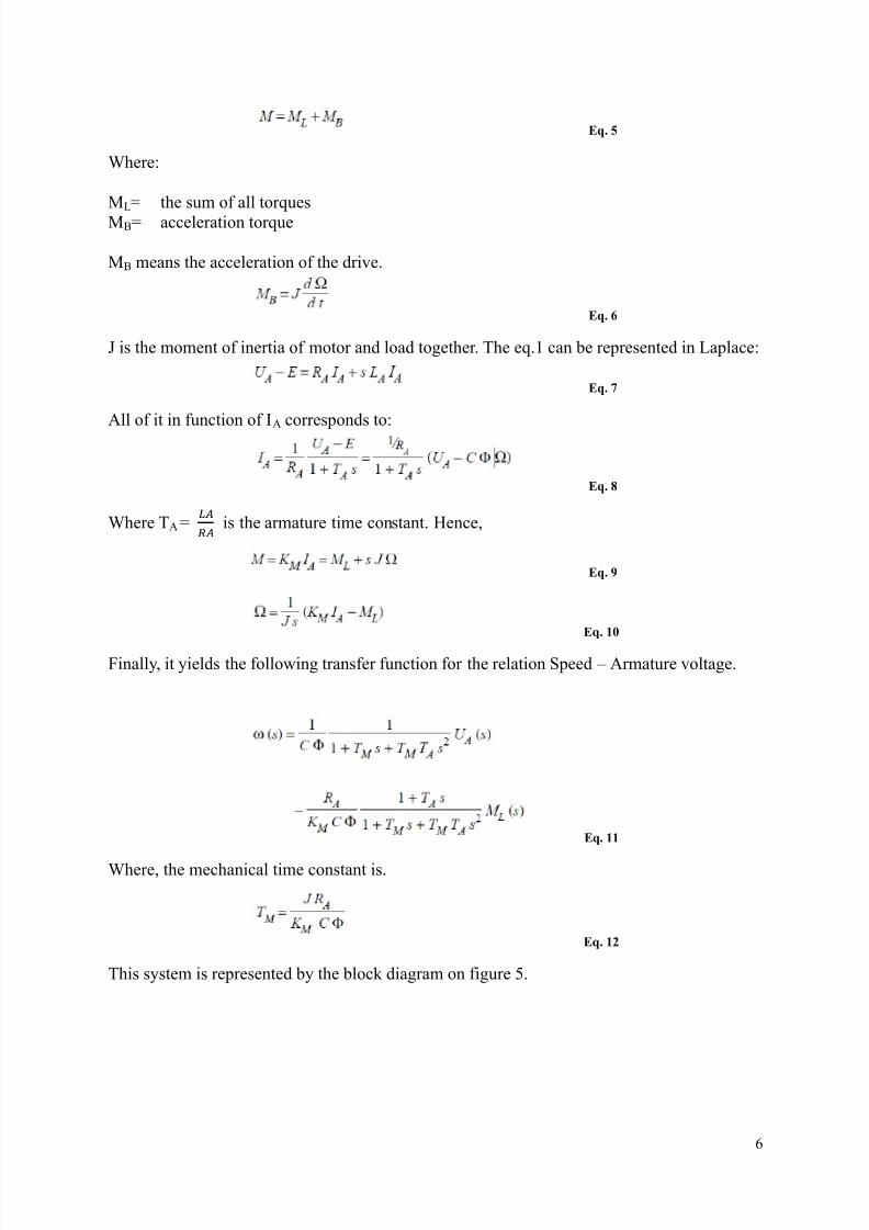
Eq. 5

Where:

ML= the sum of all torques

MB= acceleration torque

MB means the acceleration of the drive.

Eq. 6

J is the moment of inertia of motor and load together. The eq.1 can be represented in Laplace:

Eq. 7

All of it in function of IA corresponds to:

Eq. 8

Where TA =

is the armature time constant. Hence,

Eq. 9

Eq. 10

Finally, it yields the following transfer function for the relation Speed – Armature voltage.

Eq. 11

Where, the mechanical time constant is.

Eq. 12

This system is represented by the block diagram on figure 5.



7

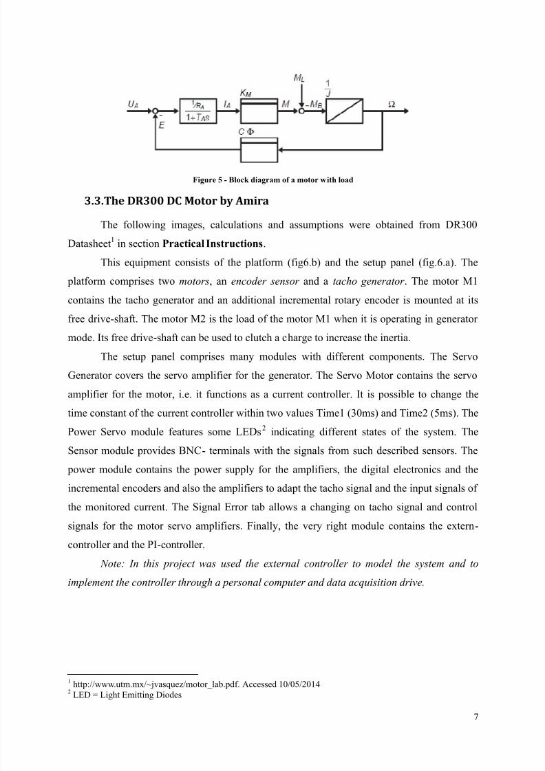
Figure 5 - Block diagram of a motor with load

3.3.

The DR300 DC Motor by Amira

The following images, calculations and assumptions were obtained from DR300

Datasheet1 in section Practical Instructions.

This equipment consists of the platform (fig6.b) and the setup panel (fig.6.a). The

platform comprises two motors, an encoder sensor and a tacho generator . The motor M1

contains the tacho generator and an additional incremental rotary encoder is mounted at its

free drive-shaft. The motor M2 is the load of the motor M1 when it is operating in generator

mode. Its free drive-shaft can be used to clutch a charge to increase the inertia.

The setup panel comprises many modules with different components. The Servo

Generator covers the servo amplifier for the generator. The Servo Motor contains the servo

amplifier for the motor, i.e. it functions as a current controller. It is possible to change the

time constant of the current controller within two values Time1 (30ms) and Time2 (5ms). The

Power Servo module features some LEDs2 indicating different states of the system. The

Sensor module provides BNC- terminals with the signals from such described sensors. The

power module contains the power supply for the amplifiers, the digital electronics and the

incremental encoders and also the amplifiers to adapt the tacho signal and the input signals of

the monitored current. The Signal Error tab allows a changing on tacho signal and control

signals for the motor servo amplifiers. Finally, the very right module contains the extern-

controller and the PI-controller.

Note: In this project was used the external controller to model the system and to

implement the controller through a personal computer and data acquisition drive.

1 http://www.utm.mx/~jvasquez/motor_lab.pdf. Accessed 10/05/2014

2 LED = Light Emitting Diodes

http://www.utm.mx/~jvasquez/motor_lab.pdf

http://www.utm.mx/~jvasquez/motor_lab.pdf



9

Therefore the Current controller is represented as follows.

Figure 9 – Current control loop

As usually TM >>TA, the feedback will have a large delay in comparison to the

armature loop. So this feedback can be neglected for an evaluation of the dynamic behavior.

Figure 10 - Current control loop simplified

Since the plant includes no integral portion, a PI controller was chosen to reach a

steady state precision. The motor M1 is controlled by a servo amplifier and has input range

from -10 to 10volt with an amplification of 0.4A/V. It behaves like a first order lag with time

constants Time1 (0.03s) or Time2 (0.005s).

Eq. 13

From figure 8, there is a gain

Cф after this control loop. Hence, eq.11 turns the

following.

Eq. 14

The open loop system is eventually represented by figure 11.

Figure 11 - Open loop System



10

4. Materials & Methods

In this project was utilized the following materials:

Amira DR300 DC Motor

Tektronix TDS 410A Digitizing Oscilloscope National Instruments TBX-68 DAQ Driver

TTi El302 Single power Supply

TTi TG215 2Mhz Function Generator

Male to Male 50Ω BNC Cables

Male to Alligator 50Ω BNC Cables

1mm Threads

Matlab 2011a and Simulink Software

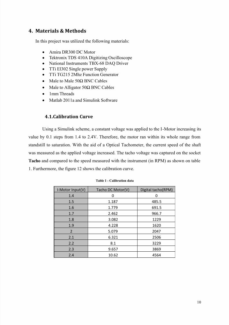
4.1.

Calibration Curve

Using a Simulink scheme, a constant voltage was applied to the I-Motor increasing its

value by 0.1 steps from 1.4 to 2.4V. Therefore, the motor ran within its whole range from

standstill to saturation. With the aid of a Optical Tachometer, the current speed of the shaft

was measured as the applied voltage increased. The tacho voltage was captured on the socket

Tacho and compared to the speed measured with the instrument (in RPM) as shown on table

1. Furthermore, the figure 12 shows the calibration curve.

Table 1 - Calibration data

I-Motor Input(V) Tacho DC Motor(V) Digital tacho(RPM)

1.4 0 0

1.5 1.187 485.5

1.6 1.779 691.5

1.7 2.462 966.7

1.8 3.082 1229

1.9 4.228 1620

2 5.079 2047

2.1 6.321 2506

2.2 8.1 3229

2.3 9.657 3869

2.4 10.62 4564



11

Figure 12 - Calibration curve

4.2.

System Modelling

In order to find out the region of linearity of the DC motor, the steady state output

voltage from the Tacho was measured while applying voltage on I – Motor (IM) input. The

figure 12 shows the motor’s response for a respective voltage application on No Load

operation.

Figure 13 - Linearity Curve

The figure shows the system is linear on the region [1.55, 2.21] (V) applied to the I-

Motor socket, i.e. the system’s response is predictable inside this region and is controllable.

RPM = 415.4V - 55.17

-1000

0

1000

2000

3000

4000

5000

0 2 4 6 8 10 12

T a c h o R P

M

Tacho Voltage(V)



12

The data acquisition is performed with a DAQ3 driver 68 pins manufactured by

National Instruments. The Servo Motor was set to Time2, which is the optimal response, with

about 0.005s delay (according to datasheet). The BNC cables are arranged on DAQ as

follows.

Figure 14 - NI DAQ TBX-68 arrangement for System Modelling

A 0.2 V step with 1.6V offset, i.e. 1.8 to 2V was applied to the system in order to

obtain its response within the linear region. The data was treated on MATLAB and the open

loop response has the characteristics shown on figure 15.

Figure 15 - Open-loop Response

The amplitude of response is in Volts for better presentation of characteristics. Using

the tool ident() on Matlab, the first and second order transfer functions were found out.

The first order model represented by G1a has gain kss = 11.44, time constant τ =

1.67s and time delay τd = 0.028s.

3 DAQ = Data Acquisition



13

() = .

.+−.

Eq. 15

The time delay represents less than 2% of the system’s time constant, thereby it is

negligible.

The second order model is represented by G2a.

() = .

.+.+ Eq. 16

The normalized transfer function is shown.

() = .

+.+. Eq. 17

Whose gain is kss=11.44, natural frequency ωn=1.4 and damping coefficient ξ=1.37.

4.3.

System Modelling Validation

In order to validate the models, the system was tried on closed loop with proportional

controller K=2. Applied 2000RPM offset for 20 seconds followed by 1000RPM step, in order

to put the motor on the linear region. Therefore, the region analyzed is on step 2000 to

3000RPM. The same was done with the open loop models and compared to the real system

with Matlab, as shown on figure 16.

Figure 16 - Open Loop Validation

The responses diverges dramatically thereby those transfer functions cannot describe properly



14

the motor. Then, the parameters for the first and second order transfer function were changed

manually to turn them better suitable to the real response. Eventually, the transfer functions

which better describe the DC motor on closed loop are G1b and G2b as follows.

() =

.

.+ −.

Eq. 18

The first order model represented by G1b has gain kss = 8.44, time constant τ = 1.47s

and time delay τd = 0.006s.

() =

+.+ Eq. 19

Whose gain is kss=337, natural frequency ωn= 6.32 and damping coefficient ξ=4.26.

The first and second order models were compared as shown on figure 17. The functions

represent the conversion between RPM to Volt (Fcn3) and back from Volt to RPM (Fcn, Fcn1

and Fcn2). The constant 1.5 is the minimal voltage necessary to put the engine on motion, as

shown on figure 13. This value is subtracted from the models in order to have the responses

matched.

Figure 17 - Closed loop models comparison on Simulink

The figure 18 presents the closed loop validation for the models G1b and G2b.

Figure 18 - Closed loop validation



15

5. Results & Discussion

5.1. System Permanence

The motor has many variables that can change its behavior over time. The friction

coefficient, for example, has different values when cold and when warm. Also, the output

sockets can get out of calibration as devices get older. To test the systems “permanence” or

“continuity over time”, the motor was put on operation continuously for different periods in

closed loop with a proportional controller K=2. The figure 19 shows the scheme.

Figure 19 – Permanence experiment Simulink scheme

A constant 8V (or 3323RPM) offset was applied for 20 seconds followed by 1V (or

415RPM) step for more 20 seconds. The whole cycle lasts 40 seconds and was repeated

several times, so that the 30th test is after 30*40= 1200s = 20 min motor running. The tacho

output for 6 different times are shown on figure 20.

Figure 20 - Output for different times



16

The figure 21 shows the change on control signal for the same reference step.

Figure 21 - Control Signal for different times

The system’s behavior changes over time, so that its gain goes from 11.44

(4700RPM/V) on cold state to 14.3 V/V (5850 RPM/V) after 20 minutes. A better transfer

function is to be worked out to describe the system. Using the average response on 9 th test,

the new model G2c was figured out.

() =

+.+. Eq. 20

Whose gain is kss=10.17, natural frequency ωn = 5.34 and damping coefficient ξ = 5.76.

5.2.

Control Design

The BNC cables are arranged on DAQ as follows.

Figure 22 - NI DAQ TBX-68 arrangement for System Control

To design a controller, it is necessary to set requirements. As the settling time for this

system is about 8.4s and the time delay is negligible, a more demanding settling time can be

required. The system has to be precise, i.e. with no steady state error and have a reasonable

overshoot. Therefore, the requirements for the controlled system are:

-

Steady-state error = 0

-

Percentage overshoot< 10% -

Settling time =1s



17

The desirable time constant of response under these requirements is about τd=1/3 =

0.33s. Therefore, for a first order response the closed loop pole should be placed at nearly p d.

In this case, there are 3 poles, but the one closest to the origin will overrule the others.

=

=

. = Eq. 21

The controller is to be designed through sisotool on Matlab. A real zero and an

integrator are added to the compensator in order to obtain a PI controller. Firstly, the zero has

to be placed on a manner to permit the closed loop poles to be in the position desirable. Then

the poles can be moved to get a better overshoot performance. The figure 23 shows the Root

Locus.

Figure 23 - Root Locus for C1 and G2c

Eventually, the closed loop poles were placed at p1=-42.08, p2=-17.5 and p3=-1.92.

The PI controller designed is C1.

1() = 2.836 4.88

The system would have 1 second settling time and 8.7% maximum overshoot.

5.3.

Model and controller improvement

Controller C1

Using the scheme of figure 24 in Simulink, the motor was controlled with C1 and its

response compared to the evaluated model. A 2000RPM offset is kept for 20 seconds to take



18

the motor out of standstill and stabilize it on linear region. Then a 500 RPM step is applied

for more 20 seconds. The function Fcn3 converts the reference speed from RPM to voltage

which feed the motor by the I-Motor socket. The current shaft speed is acquired from the

Tacho socket in volts. The functions Fcn and Fcn1 convert back the voltage to RPM and

show the value on the virtual scope.

Figure 24 - Control scheme for the DC motor

The response is shown on figure 25.

Figure 25 - Response for the controller C1

The motor’s response is good. Settling time of 0.62 seconds and 5% overshoot.However, if the response is much better than expected that means the model is not good

enough and more aggressive response can be required.

A new model was acquired by changing manually the previous model G2c and

making it suitable to the real response. A new model was attained G2d.

2() =390

6230

Whose gain is kss= 13, natural frequency ωn= 5.48 and damping coefficient ξ=5.65.



19

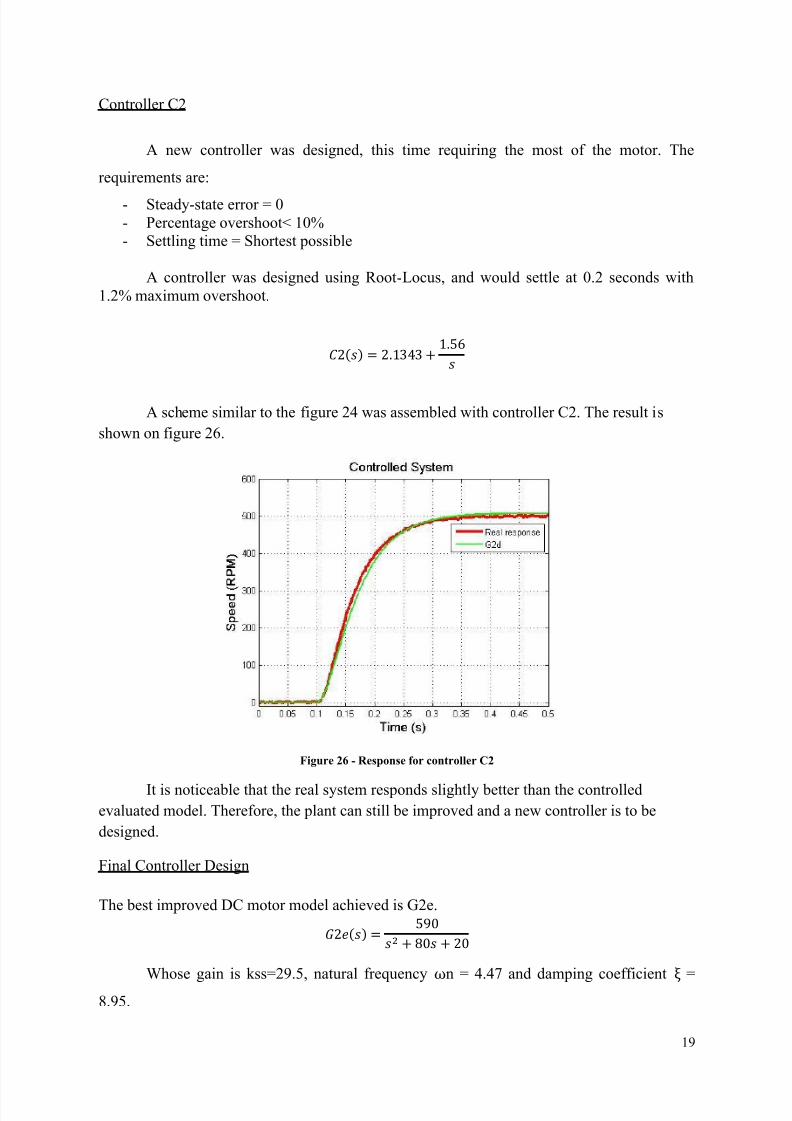
Controller C2

A new controller was designed, this time requiring the most of the motor. The

requirements are:

-


- Percentage overshoot< 10%

-

Settling time = Shortest possible

A controller was designed using Root-Locus, and would settle at 0.2 seconds with

1.2% maximum overshoot.

2() = 2.1343 1.56

A scheme similar to the figure 24 was assembled with controller C2. The result is

shown on figure 26.

Figure 26 - Response for controller C2

It is noticeable that the real system responds slightly better than the controlled

evaluated model. Therefore, the plant can still be improved and a new controller is to be

designed.

Final Controller Design

The best improved DC motor model achieved is G2e.

2() =590

80 20

Whose gain is kss=29.5, natural frequency ωn = 4.47 and damping coefficient ξ =

8.95.



20

A new controller was designed to demand the most of the equipment. The

requirements are as follows:

-


- Percentage overshoot< 10%

-

Settling time = Shortest possible

The controller would make the system to settles at about 0.1s with maximum 10% overshoot.

3() = 5.9916 7.67

The system was controlled with C3 and the result is shown on figure 27.

Figure 27 - Response for C3

The response has 9.87% overshoot and 0.11 seconds settling time. Therefore, the

controlled system has a reasonable response.

5.4. Integral Absolute Error (IAE)

The controlled system and the model diverge differently in different speeds.

Therefore, it is necessary to know how good the model represents the motor. The Integral

Absolute Error is the sum of the absolute of differences between real response and

simulation. This equation quantifies the amount of error.

= ∑| | Eq. 22

Using Simulink, the motor was controlled with the C3 controller and its response

compared to the model G2e. The reference speed was changed from 0 to 4200 RPM in

200RPM steps every 5 seconds, so that the motor had enough time to stabilize. Afterwards,

the IAE was calculated on the transient region for every setpoint, as shown on figure 28.



21

Figure 28 - IAE region of calculation

The result is shown as a bar chart on figure 29.

The plant model was figured out on the region 2000 to 2500 RPM, so it is expected

small error on this region. Good results are achieved on between 600 to 4000 RPM, what is

sensible since the motor is nearly linear on this region. Therefore, the IAE chart describes

well what is expected for the DC motor.



22

6. Conclusion

The electrical scheme was to be comprehended in order to work out a model for the rig.

However, the current controller and measuring system linked to the motor turns the processmore difficult to be controlled. Besides, the manual does not provide enough information and

explanation to some assumptions taken. Although the electrical components of the motor

were not all calculated, the box can still be controlled. And it opens a path to understand the

characteristics of the machine.

Some experimental models were figured out and continuously improved as new speed

controllers were designed. As the mechanical time constant is much bigger than the electrical

one, a second order model may be a good representation to the system. Eventually, a pretty

satisfying speed controller was designed along with a model to represent the overall system.



23

7. References

[1] National instruments NI TBX-68 Datasheet

[2] National instruments PCI 6221 Datasheet

[3] Hill, Martin. Control Fundamentals Real Time Simulink Setup Tutorial

[4] Amira.DR300 – Laboratory Setup Speed Control with Variable Load. ©Copyright

Amira 1999/2000

[5] Fuentes, Rodrigo Cardozo. Apostila de Automação Industrial. UFSM. Santa Maria –

RS, 2005.

[6] Siemens. Motores de corrente continua – Guia Rápido para uma especificação

precisa. Edição 01.2006.©Copyright Siemens LTDA.



24

Appendix

This section presents theories for the model representation of the DR 300 DC motor

by Amira. The controlled variable of the motor is the armature current, what makes the model

evaluation a challenge. Using the DR 300 Manual, it was found out two paths to represent the

plant: Block diagram and Time delay elements

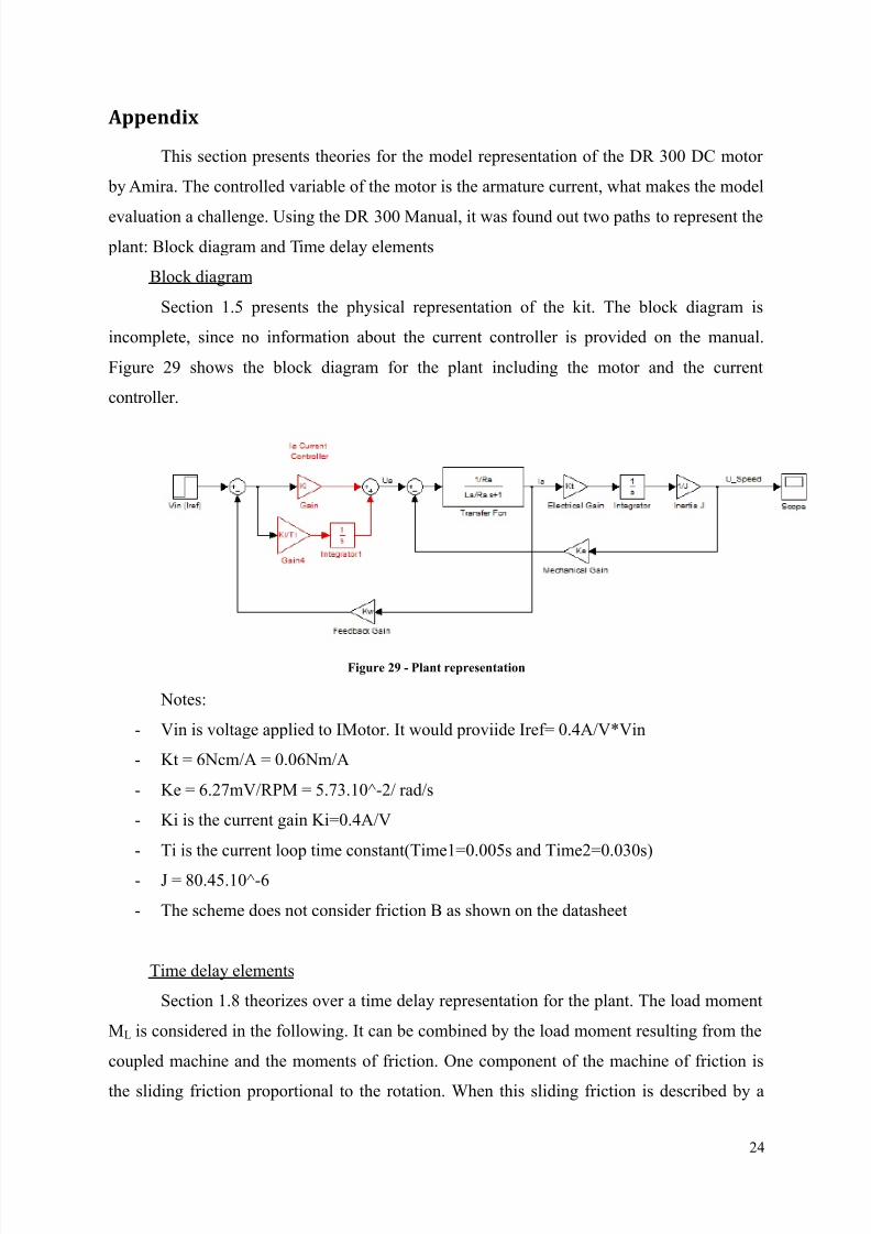
Block diagram

Section 1.5 presents the physical representation of the kit. The block diagram is

incomplete, since no information about the current controller is provided on the manual.

Figure 29 shows the block diagram for the plant including the motor and the current

controller.

Figure 29 - Plant representation

Notes:

- Vin is voltage applied to IMotor. It would proviide Iref= 0.4A/V*Vin

-

Kt = 6Ncm/A = 0.06Nm/A

- Ke = 6.27mV/RPM = 5.73.10^-2/ rad/s

- Ki is the current gain Ki=0.4A/V

- Ti is the current loop time constant(Time1=0.005s and Time2=0.030s)

- J = 80.45.10^-6

- The scheme does not consider friction B as shown on the datasheet

Time delay elements

Section 1.8 theorizes over a time delay representation for the plant. The load moment

ML is considered in the following. It can be combined by the load moment resulting from the

coupled machine and the moments of friction. One component of the machine of friction is

the sliding friction proportional to the rotation. When this sliding friction is described by a



25

feedback (K fric) of the integrator with the machine time constant TM its transfer function is

stated as

() =

1 .

= 1

. 1

. 1

The amplification factors of the current controller (Ki) and the measuring system are

known. So the overall transfer function of the current controller, the motor and the measuring

system is given by:

() =1

1 .

1

.

1

. 1

1

1

The amplification

is measurable in the open control loop. So the new machine

time constant can be determined using the measured amplification Vreal by:

=.

Then the transfer function of the open speed control loop is:

() =

(1 )(1 )(1 )

All parameters have to be calculated, as follows:

The Eq.12 give us:

= .

Ф =

80.45. 10−3.13

0.06.0.06 = 70

From Eq.15, the plant amplification is Vreal= 11.44V/V = 11.44*(415.4)-50.13

RPM/V= 4700RPM/V, with time constant.

=0.07.4700

200 = 1.645

The meaning of Tmess was not explained, so it was assumed to be the old time

constant. Tmess=0.07s



The resulting transfer function of the system is:

() =4700

0.01353 2. 722 3.295 1

The model Go was compared to G2a from Eq.17 on Simulink. The result is shown on

figure 30.

Figure 30 - Comparison between theoretical and experimental models

motor control - project research cit

Documents