motor gasoline model - energy information administration

U.S. Energy Information Administration— November 2011 Motor Gasoline Consumption Module - Short-Term Energy Outlook Model Documentation

1

Motor Gasoline Consumption Module

Short‐Term Energy Outlook Model

Table of Contents

1. Overview .................................................................................................................................. 2

2. Data sources ............................................................................................................................. 4

3. Variable naming convention ................................................................................................. 6

4. Motor gasoline consumption module equations ................................................................ 8

A. Highway‐related motor gasoline consumption ............................................................ 8

1. Vehicle miles traveled .................................................................................................... 9

2. Fuel efficiency ................................................................................................................ 10

3. Highway travel cost per mile ...................................................................................... 11

B. Non‐highway‐related motor gasoline consumption ................................................... 11

5. Forecast evaluations ............................................................................................................. 12

Appendix A. Variable definitions ........................................................................................... 17

Appendix B. Eviews motor gasoline consumption module code ...................................... 18

Appendix C. Regression Results ............................................................................................. 19


2

1. Overview

The motor gasoline consumption module of the Short‐Term Energy Outlook (STEO)

model is designed to provide forecasts of domestic motor gasoline consumption. The

frequency of the STEO model is monthly and the model equations are used to produce

monthly forecasts over a 13‐to‐24 month horizon (every January the STEO forecast is

extended through December of the following year).

The STEO model contains over 2,000 equations, of which about 450 are estimated

regression equations. The regression equations are estimated and the forecast models

are solved using EViews Econometric Software (Quantitative Micro Software, LLC).

The motor gasoline consumption module, which is documented in this report, contains

12 equations, of which 3 are estimated regression equations. Some input variables to

the motor gasoline consumption module are exogenous, coming from other modules in

the STEO model or forecasts produced by other organizations (e.g., weather forecasts

from the National Oceanic and Atmospheric Administration).

Gasoline ʺconsumptionʺ refers to deliveries from primary suppliers, which include

refineries, blenders, pipelines, and bulk terminals. 1 Deliveries therefore differ from

retail sales. Between 1999 and 2010, total motor gasoline consumption growth averaged

0.7 percent per year. Motor gasoline consumption is highly seasonal, as shown in

Figure 1. Total gasoline consumption, which averaged 8.99 million barrels per day

(bbl/d) during 2010, ranged from a low of 8.52 million bbl/d in January 2010 to a high of

9.36 million bbl/d in August 2010.

1 In EIA terminology, deliveries are also referred to as “products supplied,” “shipments,” and

“disappearance from supply.”


3

Figure 1. Motor gasoline consumption, January 1994 – December 2010.

The motor gasoline consumption module derives total gasoline consumption from

separate estimates of highway‐related and non‐highway‐related gasoline consumption

(Figure 2). Highway‐related consumption, which accounted for 97 percent of the total

in 2009, includes usage by households; public transportation systems; and commercial,

institutional, and government entities. Non‐highway consumption includes usage by

recreational boats and agricultural and industrial (including construction) entities.

6

7

8

9

10

Jan‐94 Jan‐96 Jan‐98 Jan‐00 Jan‐02 Jan‐04 Jan‐06 Jan‐08 Jan‐10

Source: EIA, Petroleum Supply Monthly.

Million barrels per day


4

Figure 2. Flow chart of motor gasoline consumption module.

2. Data sources

The sources for monthly total motor gasoline consumption are:

the EIA Weekly Petroleum Status Report for estimated monthly‐from‐weekly

volumes for the two most recent months;

the EIA Petroleum Supply Monthly for preliminary monthly data;

the EIA Petroleum Supply Annual for revised final monthly data.

Separate series for highway and non‐highway motor gasoline consumption are not

available at a monthly frequency. Annual highway and non‐highway data are

published in Highway Statistics, Table MF24, Federal Highway Administration (FHwA),

Department of Transportation. For each calendar year, monthly highway and non‐

highway motor gasoline consumption figures are derived by multiplying their

respective annual shares by the monthly total gasoline consumption. Because of the

impacts of winter weather, spring‐time crop planting, fall‐season harvesting, and

summer recreational activity, seasonal patterns for non‐highway usage are assumed to


5

be similar to those for highway consumption. For example, the highway share of total

motor gasoline consumption for 2003 was 97 percent. In August 2003 total gasoline

consumption according to the Petroleum Supply Annual was 9.411 million bbl/d. Thus,

highway demand for that month is estimated to be 9.129 million bbl/d (= 0.97 x 9.411).

Non‐highway demand, 0.282 million bbl/d, accounts for the remaining 3 percent of total

demand.

The Federal Highway Administration reports total vehicle miles traveled in the

monthly Traffic Volume Trends report

(http://www.fhwa.dot.gov/ohim/tvtw/tvtpage.cfm). Traffic volume trends are based on

hourly traffic count data collected at approximately 4,000 continuous traffic counting

locations nationwide, which are used to determine the percent change in traffic for the

current month compared with the same month in the previous year. This percent

change is applied to the travel for the same month of the previous year to obtain an

estimate of travel for the current month. Because of the limited sample sizes and the

inclusion of both gasoline‐ and diesel‐fueled vehicles in the traffic counts, vehicle miles

traveled should only be interpreted as a proxy for gasoline‐fueled vehicle travel.

Average gasoline‐vehicle highway fuel efficiency, in miles per gallon, is calculated as

total vehicle miles traveled divided by highway gasoline consumption (Equation 1):

MPG (MVVMPUS / MGHCPUS) / 42 (1)

where,

MPG = gasoline‐related highway fuel efficiency, miles per gallon;

MVVMPUS = vehicles miles traveled, million miles per day;

MGHCPUS = highway consumption of motor gasoline, million barrels per day.

Retail motor gasoline prices are published in the EIA Weekly Petroleum Status Report.

Monthly prices are calculated as a simple average of the weekly prices.

The gasoline consumption module uses macroeconomic variables such as real personal

disposable income, unemployment, and the Consumer Price Index as explanatory

variables in the generation of forecasts. The macroeconomic forecasts are generated

using models developed by IHS Global Insight Inc. (GI). GI updates its national

macroeconomic forecasts monthly using its model of the U.S. economy. EIA re‐runs the

GI model to produce macroeconomic forecasts that are consistent with the STEO energy

price forecasts.


6

Historical data for heating degree‐days are obtained from the National Oceanic and

Atmospheric Administration (NOAA).2 NOAA also publishes forecasts of population‐

weighted regional heating degree‐days up to 14 months out. In cases where the STEO

forecast horizon goes beyond the NOAA forecast period, “normal” values are used.

NOAA reports normal heating degree‐days as the average of the 30‐year period 1971‐

2000. However, the STEO model uses a corrected degree‐day normal that adjusts for

the warming trend that began around 1965 (The Impact of Temperature Trends on Short‐

Term Energy Demand).

3. Variable naming convention

Over 2,000 variables are used in the STEO model for estimation, simulation, and report

writing. Most of these variables follow a similar naming convention. The following

table shows an example of this convention using total motor gasoline consumption:

Characters MG TC P US

Positions 1 and 2 3 and 4 5 6 and 7

Categories Energy or energy‐

related concept

Energy activity

or consumption

end‐use sector

Type of data

Geographic area

or special

equation factor

In this example, MGTCPUS is the identifying code for motor gasoline (MG) total

consumption (TC) in physical units (P) in the United States (US). A more detailed

breakdown of naming classifications for the motor gasoline consumption module is

shown below:

Energy or energy‐related concepts:

MG = motor gasoline

MV = motor vehicles

ZW = weather

Energy activity or consumption end‐use sectors:

2 Heating degree‐days (HDD), a measure of the relative coldness of a location, is calculated as the

deviation of daily average temperature below 65 degrees; HDD = 0 if average temperature exceeds 65.


7

HC = highway consumption

NC = non‐highway consumption

TC = total consumption

RA = regular grade gasoline

HD = heating degree days

VM = vehicle miles traveled

Type of data:

D = deviations from normal (e.g., heating degree days)

P = physical units

R = nominal retail price per standardized physical unit, including taxes

Geographic identification or special equation factor:

US = United States

Some series may be seasonally adjusted using the Census X‐11 method. The seasonally

adjusted series has an “_SA” appended to the end of the variable name, such as

MGTCPUS_SA for seasonally‐adjusted motor gasoline consumption. The seasonal

factor series has an “_SF” appended to the end of the variable name, such as

MGTCPUS_SF for motor gasoline consumption seasonal factors.

Regression equations with series that are not seasonally adjusted may include monthly

dummy variables to capture the normal seasonality in the data series. For example,

JAN equals 1 for every January in the time series and is equal to 0 in every other month.

Dummy variables for specific months may also be included in regression equations

because the observed data may be outliers because of infrequent and unpredictable

events such as hurricanes, survey error, or other factors. Generally, dummy variables

are introduced when the absolute value of the estimated regression error is more than 2

times the standard error of the regression (the standard error of the regression is a

summary measure based on the estimated variance of the residuals). No attempt was

made to identify the market or survey factors that may have contributed to the

identified outliers.

Dummy variables for specific months are generally designated Dyymm, where yy = the

last two digits of the year and mm = the number of the month (from “01” for January to

“12” for December). Thus, a monthly dummy variable for March 2002 would be D0203

(i.e., D0203 = 1 if March 2002, = 0 otherwise).


8

Dummy variables for specific years are designated Dyy, where yy = the last two digits

of the year. Thus, a dummy variable for all months of 2002 would be D02 (i.e., D02= 1 if

January through December 2002, 0 otherwise). A dummy variable might also be

included in an equation to show a structural shift in the relationship between two time

periods. Generally, these type of shifts are modeled using dummy variables designated

DxxON, where xx = the last two digits of the years at the beginning of the latter shift

period. For example, D03ON = 1 for January 2003 and all months after that date, = 0 for

all months prior to 2003.

4. Motor gasoline consumption module equations

Total motor gasoline consumption is the sum of highway and non‐highway

consumption (Equation 2):

MGTCPUS MGHCPUS + MGNCPUS (2)

Where,

MGHCPUS = highway motor gasoline consumption, million barrels per day;

MGNCPUS = non‐highway motor gasoline consumption, million barrels per day;

MGTCPUS = total motor gasoline consumption, million barrels per day.

A. Highway‐related motor gasoline consumption

Projections for highway motor‐gasoline consumption require forecasts of both vehicle

miles traveled and average vehicle fuel efficiencies. These forecasts are calculated

according to the identity in equation (3), which uses forecasts generated from the

regression equations (4) and (5):

MGHCPUS MVVMPUS / (MPG * 42) (3)

Where,

MGHCPUS = highway motor gasoline consumption, million barrels per day;

MPG = average vehicle fuel efficiency, miles per gallon;

MVVMPUS = vehicle miles traveled, million miles per day.


9

1. Vehicle miles traveled

Estimates for seasonally‐adjusted per‐capita vehicle miles traveled are derived from

regression equation (4), which is estimated using ordinary least squares:

log(MVVMPUS_ SA/POP ) = a0 + a1 log(YD87OUS/POP) (4)

+ a2 log(CPM_SA)

+ a3 log(XRUNR)

+ a4 log(ZWHDDUS1/ZSAJQUS

Where,

CPM_SA = inflation‐adjusted motor gasoline cost, cents per mile, seasonally

adjusted;

MVVMPUS_SA = vehicle miles traveled, million miles per day seasonally

adjusted;

POP = total U.S. population, millions;

YD87OUS = real personal disposable income, billion chained 2005 dollars;

XRUNR = rate of unemployment, percent;

ZWHDDUS1 = population‐weighted heating‐degree day deviations from normal

for December, January and February that have positive values and 0

otherwise for all months;

ZSAJQUS = number of days in each month.

Highway travel per capita is a positive function of real personal disposable income

(YD87OUS) per capita. Because the equation is in logs, the estimated coefficient is an

approximate measure of the short‐run income elasticity of highway‐related travel and

real income. However, some of the travel response to income may also be captured by

the negative relationship between travel and the unemployment rate (XRUNR).

Highway travel is also a negative function of the seasonally‐adjusted real cost of

gasoline (CPM_SA), expressed in cents per mile (equation 6). Again, because the

equation is in logs, the estimated coefficient is an approximation of the short‐run price

elasticity of highway‐related travel and price. However, the elasticity implied by this

estimated coefficient may be understated because prices may affect real household

income and some of the elasticity may be captured by the income coefficient.

The ZWHDDUS1/ZSAJQUS weather term captures the effects of colder‐than‐normal

weather during the winter months, which may depress highway travel.


10

2. Fuel efficiency

Estimates for seasonally‐adjusted motor gasoline‐related fuel efficiency are derived

from regression equation (5), which is estimated using ordinary least squares:

MPG_SA = b0 + b1 (EOTCPUS_SA/MGTCPUS_SA) (5)

+ b2 (ZWHDDUS1/ZSAJQUS)

+ b3 TREND Where,

EOTCPUS_SA = ethanol blended into gasoline, million barrels per day,

seasonally adjusted;

MPG_SA = motor gasoline‐related fleet‐wide fuel efficiency, miles per gallon,


TREND = vector of integers starting at 1 for the first observation of the estimation

period (January, 1998), incrementing by 1 for each subsequent

observation;

ZWHDDUS1 = population‐weighted heating‐degree day deviations from normal

for December, January and February observations which have positive

values and 0 otherwise;

ZSAJQUS = number of days in each month.

The equation includes a trend variable, which captures the trend in increasing average

fuel efficiency, such as related to increasing corporate average fuel economy (CAFE)

standards.

Average vehicle fuel efficiency is negatively related to the ethanol volumetric share in

the gasoline pool. Ethanol contains about 70 percent of the energy content of

conventional gasoline. Consequently, we might expect a 0.3 percent reduction in

average fuel efficiency with each 1 percent increase in the volumetric share of ethanol in

the gasoline pool. The ethanol consumption forecast comes from the oxygenates

module of the STEO model. Note that caution should be exercised in setting the

estimation period of this equation because of the possible strong multicollinearity

between the ethanol share and the time trend variable

The ZWHDDUS1/ZSAJQUS weather term captures the effects of colder‐than‐normal

weather episodes.


11

3. Highway travel cost per mile

The inflation‐adjusted cost per mile, CPM, is calculated using equation (6):

CPM (MGRARUS / CICPIUS) / MPG (6)

Where,

CPM = inflation‐adjusted motor gasoline cost, cents per mile;

MGRARUS = monthly average retail regular‐grade motor gasoline price

including taxes, cents per gallon;

CICPIUS = consumer price index for all urban consumers, 1982‐1984=1.00;

MPG = motor gasoline‐related highway fuel efficiency, miles per gallon.

The seasonally‐adjusted cost per mile (CPM_SA) is calculated by dividing the nominal

cost by the seasonal factor (CPM_SF) derived from the Census X‐11 procedure (equation

7):

CPM_SA = CPM / CPM_SF (7)

B. Non‐highway‐related motor gasoline consumption

Forecasts for seasonally‐adjusted per‐capita non‐highway motor gasoline consumption

are derived from regression equation (8), which is estimated using ordinary least

squares

log(MGNCPUS_ SA/POP) = c0 + c1 log(YD87OUS/POP) (8)

+ c2 MGNCPUS_SA(‐1)/POP(‐1)

+ dummy variables

Where,

MGNCPUS_SA = non‐highway motor gasoline usage, million barrels per day,


POP = total U.S. resident population, millions;


12

YD87OUS = inflation‐adjusted real personal disposable income, billion chained

2005 dollars.

5. Forecast evaluations

In order to evaluate the reliability of the forecasts, we generated out‐of‐sample forecasts

and calculated forecast errors. Each equation was estimated through December 2008.

Dynamic forecasts were then generated for the period January 2009 through December

2010 using each regression equation. The forecasts are then compared with the actual

outcomes.

Table 3 reports the differences between the annual averages of the out‐of‐sample

dynamic forecasts and actual values for 2009 and 2010. A forecast for total gasoline

consumption is derived from the forecasts of highway‐related consumption (from miles

traveled and average vehicle fuel efficiency) and non‐highway‐related consumption.

The out‐of‐sample forecast of total gasoline consumption for 2009 was about 0.4 percent

lower than actual consumption, while the forecast for 2010 was about 0.6 percent higher

than actual consumption. The primary source of forecast error in 2009 was vehicle

miles traveled, while the primary source of error in the 2010 forecast was average

vehicle fuel efficiency.

Table 1. Actual versus out‐of‐sample consumption forecasts, annual averages.

2009 2010

Equation Actual Forecast Actual Forecast

MVVMPUS_SA 8,159 8,103 8,212 8,220

MPG_SA 22.13 22.10 22.18 22.11

MGHCPUS * 8.767 8.720 8.784 8.849

MGNCPUS 0.230 0.232 0.251 0.243

MGTCPUS * 8.997 8.958 9.034 9.092

* MGHCPUS forecast calculated based on forecasts of MVVMPUS_SA and MPG_SA.

MGTCPUS forecast calculated based on forecasts of MGHCPUS and MGNCPUS.

Source: EIA, Short‐Term Energy Outlook model.

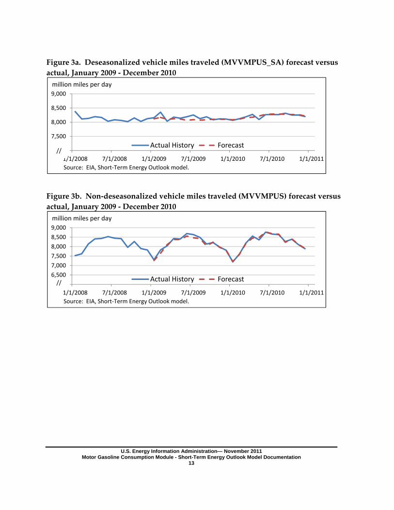
The differences between the monthly out‐of‐sample forecasts and actual values are

shown in Figures 3 through 6. The forecast of highway‐related gasoline consumption

can be derived from the forecasts of vehicle miles traveled and average vehicle fuel

efficiency and are compared with actual consumption in Figure 5.


13

Figure 3a. Deseasonalized vehicle miles traveled (MVVMPUS_SA) forecast versus

actual, January 2009 ‐ December 2010

Figure 3b. Non‐deseasonalized vehicle miles traveled (MVVMPUS) forecast versus


7,000

7,500

8,000

8,500

9,000

1/1/2008 7/1/2008 1/1/2009 7/1/2009 1/1/2010 7/1/2010 1/1/2011

Actual History Forecast

million miles per day


//

6,000

6,500

7,000

7,500

8,000

8,500

9,000

1/1/2008 7/1/2008 1/1/2009 7/1/2009 1/1/2010 7/1/2010 1/1/2011


million miles per day


//


14

Figure 4a. Deseasonalized average vehicle fuel efficiency (MPG_SA) forecast versus


Figure 4b. Non‐deseasonalized average vehicle fuel efficiency (MPG_SA) forecast

versus actual, January 2009 ‐ December 2010

19

20

21

22

23

24

1/1/2008 7/1/2008 1/1/2009 7/1/2009 1/1/2010 7/1/2010 1/1/2011


miles per gallon


19

20

21

22

23

24

1/1/2008 7/1/2008 1/1/2009 7/1/2009 1/1/2010 7/1/2010 1/1/2011


miles per gallon



15

Figure 5. Non‐deseasonalized highway‐related motor gasoline consumption

(MGHCPUS) forecast versus actual, January 2009 – December 2010.

Figure 6. Non‐deseasonalized non‐highway motor gasoline consumption

(MGNCPUS) forecast versus actual, January 2009 ‐ December 2010.

Table 5 reports summary forecast error statistics for each regression equation. The Root

Mean Squared Error and the Mean Absolute Error depend on the scale of the dependent

variable. These are generally used as relative measures to compare forecasts for the

same series using different models; the smaller the error, the better the forecasting

ability of that model.

The mean absolute percentage error (MAPE) and the Theil inequality coefficient are

invariant to scale. The smaller the values the better the model fit. The Theil inequality

coefficient always lies between zero and one, where zero indicates a perfect fit. The

Theil inequality coefficient is broken out into bias, variance, and covariance

7.88.08.28.48.68.89.09.29.4

1/1/2008 7/1/2008 1/1/2009 7/1/2009 1/1/2010 7/1/2010 1/1/2011


million barrels per day


0.00

0.05

0.10

0.15

0.20

0.25

0.30

0.35

1/1/2008 7/1/2008 1/1/2009 7/1/2009 1/1/2010 7/1/2010 1/1/2011


million barrels per day



16

proportions, which sum to 1. The bias proportion indicates how far the mean of the

forecast is from the mean of the actual series signaling systematic error. The variance

proportion indicates how far the variation of the forecast is from the variation of the

actual series. This will be high if the actual data fluctuates significantly but the forecast

fails to track these variations from the mean. The covariance proportion measures the

remaining unsystematic forecasting errors. For a “good” forecast the bias and variance

proportions should be small with most of the forecast error concentrated in the

covariance proportion.

The bias proportion for each forecast series is small. The variance proportions for

vehicle miles traveled and average vehicle fuel efficiency are large because the errors

are calculated for deseasonalized series that have significant seasonal swings (Figures

3b and 4b).

Table 2. Regional Consumption Out‐of‐Sample Simulation Error Statistics

Highway miles

traveled

Average

vehicle

fuel

efficiency

Off‐highway

gasoline

consumption

MVVMPUS_SA MPG_SA MGNCPUS_SA

Root Mean Squared Error 69.2 0.196 0.029

Mean Absolute Error 52.4 0.161 0.022

Mean Absolute Percentage Error 0.642 0.725 9.89

Theil Inequality Coefficient 0.0042 0.004 0.061

Bias Proportion 0.063 0.065 0.006

Variance Proportion 0.312 0.262 0.735

Covariance Proportion 0.625 0.673 0.258

Forecast period = January 2009 – December 2010


17

Appendix A. Variable definitions

Table A1. Variable definitions, units, and sources Sources

Variable Name Units Definition History Forecast

CICPIUS Index Consumer price index, all urban consumers (1982‐1984=1.00) GI GI

CPM CPG Real cost per mile STEO STEO

CPM_SA CPG Real cost per mile, seasonally adjusted STEO STEO

CPM_SF Index Real cost per mile, seasonal adjustment factor STEO STEO

Dyy Integer = 1 if year (yy), 0 otherwise ‐‐ ‐‐

Dyymm Integer = 1 if month (mm) and year (yy), 0 otherwise ‐‐ ‐‐

DyyON Integer = 1 if year (yy) or later, 0 otherwise ‐‐ ‐‐

EOTCPUS_SA MMBD Ethanol consumption, seasonally adjusted PSM STF

MGHCPUS MMBD Highway‐related gasoline consumption STEO STEO

MGHCPUS_SA MMBD Highway‐related gasoline consumption, seasonally adjusted STEO STEO

MGHCPUS_SF Index Highway‐related gasoline consumption, seasonal adjustment factor STEO STEO

MGNCPUS MMBD Non‐highway‐related gasoline consumption STEO STEO

MGNCPUS_SA MMBD Non‐highway‐related gasoline consumption, seasonally adjusted STEO STEO

MGNCPUS_SF Index Non‐highway‐related gasoline consumption, seasonal adjustment factor STEO STEO

MGTCPUS MMBD Total motor gasoline consumption WPSR/PSM STEO

MGTCPUS_SA MMBD Total motor gasoline consumption, seasonally adjusted STEO STEO

MGTCPUS_SF Index Total motor gasoline consumption, seasonal adjustment factor STEO STEO

MPG MPG Average vehicle fuel efficiency STEO STEO

MPG _SA MPG Average vehicle fuel efficiency, seasonally adjusted STEO STEO

MPG _SF Index Average vehicle fuel efficiency, seasonal adjustment factor STEO STEO

MVVMPUS MPG Vehicle miles traveled FHWA STEO

MVVMPUS _SA MPG Vehicle miles traveled, seasonally adjusted STEO STEO

MVVMPUS _SF Index Vehicle miles traveled, seasonal adjustment factor STEO STEO

POP MM U.S. resident population GI GI

TREND Integer Time trend variable ‐‐ ‐‐

YD87OUS Real Disposable Personal Income GI GI

ZSAJQUS Integer Number of days in a month ‐‐ ‐‐

ZWHDDUS1 HDD Population‐weighted heating‐degree day deviations from normal for

December, January and February observations which have positive

values, 0 otherwise

NOAA NOAA

Table A2. Units key Table A3. Sources keyCPG Cents per gallon FHWA Federal Highway Administration

HDD Heating degree‐days GI IHS‐Global Insight macroeconomic model

Index Index value NOAA

National Oceanic and Atmospheric

Organization

Integer Number = 0 or 1 PSM Petroleum Supply Monthly

MMBD Million barrels per day STEO Short‐term Energy Outlook Model

WPSR EIA Weekly Petroleum Status Report


18

Appendix B. Eviews motor gasoline consumption module code

@IDENTITY CPM = (MGRARUS / CICPIUS) / MPG

@IDENTITY CPM_SA = CPM / CPM_SF

:EQ_MVVMPUS ‘ regression equation

@IDENTITY MVVMPUS = MVVMPUS_SA * MVVMPUS_SF

:EQ_MPG ‘ regression equation

@IDENTITY MPG = MPG_SA * MPG_SF

@IDENTITY MGHCPUS = MVVMPUS / (MPG * 42)

@IDENTITY MGHCPUS_SA = MGHCPUS / MGHCPUS_SF

:EQ_MGNC ‘ regression equation

@IDENTITY MGNCPUS = MGNCPUS_SA * MGNCPUS_SF

@IDENTITY MGTCPUS = MGHCPUS + MGNCPUS

@IDENTITY MGTCPUS_SA = MGTCPUS / MGTCPUS_SF


19

Appendix C. Regression Results

C1. Seasonally‐adjusted per‐capita motor‐gasoline‐related highway travel (million

miles per day)

Dependent Variable: LOG(MVVMPUS_SA/POP) Method: Least Squares Date: 03/18/11 Time: 16:42 Sample: 2000M01 2010M12 Included observations: 132

Variable Coefficient Std. Error t-Statistic Prob.

C 1.496890 0.158404 9.449816 0.0000 LOG(YD87OUS/POP) 0.542833 0.050203 10.81282 0.0000

LOG(CPM_SA) -0.016477 0.007421 -2.220395 0.0283 LOG(XRUNR) -0.013685 0.006421 -2.131266 0.0351

LOG(ZWHDDUS1/ZSAJQUS)*(DEC+JAN+FEB) -0.003707 0.000760 -4.874486 0.0000

D0001+D0002 -0.027045 0.007161 -3.776637 0.0002 D0003 0.025164 0.009215 2.730851 0.0073 D0402 -0.029281 0.009024 -3.244643 0.0015 D0501 -0.027150 0.009392 -2.890817 0.0046 D0712 -0.050832 0.009605 -5.291989 0.0000

D06+D07 -0.020615 0.003635 -5.671005 0.0000 D08ON -0.058540 0.004032 -14.51877 0.0000

R-squared 0.817493 Mean dependent var 3.296848 Adjusted R-squared 0.800763 S.D. dependent var 0.019979 S.E. of regression 0.008918 Akaike info criterion -6.514976 Sum squared resid 0.009544 Schwarz criterion -6.252903 Log likelihood 441.9884 Hannan-Quinn criter. -6.408481 F-statistic 48.86450 Durbin-Watson stat 1.804822 Prob(F-statistic) 0.000000


20

C2. Seasonally‐Adjusted Motor Gasoline‐Related Fuel Efficiency (miles per gallon) Dependent Variable: MPG_SA Method: Least Squares Date: 04/15/11 Time: 08:59 Sample: 1998M01 2010M12 Included observations: 156


C 21.27670 0.039129 543.7605 0.0000 EOTCPUS_SA/(MGTCPUS_SA) -5.065209 1.635948 -3.096192 0.0024

ZWHDDUS1/ZSAJQUS -0.067481 0.020809 -3.242869 0.0015 @TREND(1997:12) 0.009087 0.001013 8.970018 0.0000

D9901 -0.630684 0.219886 -2.868236 0.0048 D9911 0.672634 0.218955 3.072022 0.0025 D9912 -0.934413 0.218840 -4.269845 0.0000 D0002 -0.912622 0.218582 -4.175200 0.0001 D0106 0.560589 0.218055 2.570860 0.0112 D0402 -0.749336 0.218278 -3.432939 0.0008 D0501 -0.571338 0.218419 -2.615788 0.0099 D0712 -0.688515 0.218230 -3.155003 0.0020 D0809 0.810672 0.219855 3.687299 0.0003

R-squared 0.733598 Mean dependent var 21.77362 Adjusted R-squared 0.711243 S.D. dependent var 0.403187 S.E. of regression 0.216657 Akaike info criterion -0.141343 Sum squared resid 6.712484 Schwarz criterion 0.112811 Log likelihood 24.02477 Hannan-Quinn criter. -0.038117 F-statistic 32.81522 Durbin-Watson stat 1.574358 Prob(F-statistic) 0.000000


21

C3. Seasonally‐Adjusted Per‐Capita Non‐Highway

Motor Gasoline Demand (million barrels per day) Dependent Variable: LOG(MGNCPUS_SA/POP) Method: Least Squares Date: 04/15/11 Time: 09:14 Sample (adjusted): 1994M02 2010M12 Included observations: 203 after adjustments


C -9.125570 0.474893 -19.21605 0.0000 LOG(YD87OUS/POP) 1.196773 0.064122 18.66410 0.0000

D99 -0.174820 0.010159 -17.20844 0.0000 D00 -0.229814 0.012936 -17.76607 0.0000 D07 -0.118528 0.008367 -14.16617 0.0000 D08 -0.263087 0.014114 -18.63969 0.0000

D09ON -0.259931 0.014107 -18.42539 0.0000 LOG(MGNCPUS_SA(-1)/POP(-1)) 0.281182 0.037180 7.562675 0.0000

R-squared 0.985598 Mean dependent var -7.178820 Adjusted R-squared 0.985081 S.D. dependent var 0.162731 S.E. of regression 0.019876 Akaike info criterion -4.959962 Sum squared resid 0.077038 Schwarz criterion -4.829392 Log likelihood 511.4362 Hannan-Quinn criter. -4.907139 F-statistic 1906.441 Durbin-Watson stat 1.365461 Prob(F-statistic) 0.000000

motor gasoline model - energy information administration

Documents