APPENDIX:EPIC MRF MODEL FOR ASSESSINGMRF OPERATIONS AND COSTS

Table of ContentsTable of ContentsTable of ContentsTable of ContentsTable of Contents

Introduction A-1Model Organization A-1Model Terminology A-2Getting Started A-5Requirements for Installation A-5Navigating the Model A-5Entering Data A-6Printing A-6Saving Model Results A-6Conclusion A-6How To Read Each Table A-7Processing - Introduction A-8Background Input Table: facility Information A-8Input Table 1: Recovered Materials A-8Input Table 2: Sorting A-10Input Table 3a: Allocation of Sorting Labor A-11Input Table 3b: Allocation of Automated Sorting Station Resources A-12Input Table 4: Maximum Sustainable Sorting Rates A-13Input Table 5: Available Sorting Time A-14Input Table 6: Sorting Conveyor Belt Parameters A-15Input Table 7: Baling A-16Input Table 8: Incoming Material Storage A-17Input Table 9: Bale Storage A-18Output Table 1: Materials Received A-19Output Table 2: Establishing Processing Streams and Sort Rates A-21Output Table 3: Processing Streams A-21Output Table 4: Sorters and Sorting Stations A-22Output Table 5: Compaction and Post-processing Storage A-24Costs: Introduction A-26Input Table 1: Capital Costs A-26Input Table 2: Labor Costs A-27Input Table 3: Operating and Administrative Costs A-28Output Table 1: Unit Cost Summary A-29Cost Allocation: Introduction A-31Input/Output Table 1: Cost Allocation by Material A-31Output Table 2: Allocation by Material Groupings A-33

TABLE OF CONTENTS

A-1

INTRODUCTION

The Sorting Plastic Bottles for Recy-cling Guide was designed to identifyand summarize the factors that result inefficient and cost-effective recovery ofplastics. There are reference tables andcomparisons of operating and cost pa-rameters observed at each of the MRFsevaluated as part of the study. Thesesummaries are designed to allow facil-ity operators to compare their facilitieswith the facilities in that report.

HOWEVER, you may wish to go a stepfurther in analyzing the operations atyour MRF. Specifically, you may wishto take advantage of the EPIC MRFModel (Model), which was used as ananalytical tool during preparation of theGuide. The EPIC MRF Model is aMicrosoft Excel 5.0 spreadsheet toolthat helps you systematically analyzecertain operating and cost parametersat your MRF. A copy of the Model canbe downloaded from APC’s website atwww.plasticsresource.com/recycle, or adisk containing the model can be mailedto you by calling 1-800-2HELP-90.

As with any spreadsheet, the MRF Modelcan be divided into two components:

l Input is the data that you must col-lect to enter into the Model. To uti-lize the full capabilities of theModel, you may need to gather in-puts from plant operating reports,from accounting or financial state-ments, or from real-time measure-ments or operational tests per-formed at your MRF.

l Output is the information that iscalculated by the spreadsheetModel, based on the inputs yougather and formulas or calculationsbuilt into the Model. Output fromthe Model will highlight critical op-erating or cost parameters and shedinsight on some aspect of yourMRF’s performance.

This Guide describes the data you willneed to use the Model effectively, andexplains the Model’s input and outputtables. Note that the Model will helpyou assess not only plastics processing,but also the processing of all materialshandled at your entire facility.

MODEL ORGANIZATION

Although the Model is a simple spread-sheet with pre-programmed tables andformulas, it is quite comprehensive. Tomake most effective use of all compo-nents of the Model, and to take advan-tage of its flexibility, you must first un-derstand how it is organized.

The Model can be divided into threebroad sections:

l Processing: The sections dealingwith processing enable you to ana-lyze a variety of operational factorsthat impact the receiving, sorting,baling, storage and shipping of ma-terial at your MRF. For example,the Model assesses sorter utilizationrates, sorting conveyor belt speeds,required storage space, and otheroperating characteristics.

l Cost: In this section of the Model,you have the ability to compile capi-tal and operating costs of your fa-cility and to generate per-ton andother unit costs on a plant-wide ba-sis. The inputs for this section maybe obtained from your financialrecords, depending on how costs areaccounted for at your facility.

l Cost Allocation: This section takesthe Cost section one step further,and allows you to analyze the costsof processing each recovered ma-terial, or groups of recovered mate-rials (such as all plastics), individu-ally.

A-2

Within each of these three sectionsthere are multiple input and outputtables. In the Processing section of theModel, separate input tables have beencreated to help you identify the data re-quired to use the Model. In the Costand Cost Allocation sections of theModel, all input and output data appearon the same table; the tables are all, ineffect, both input and output tables.

How can you follow this organizationin the Excel spreadsheet? The answeris simple. For clarity, each discrete in-put and output table of the Model hasbeen located on a separate tab, or sheet,within the Excel spreadsheet. By us-ing the tabs at the bottom of the screen,you will be able to quickly peruse eachof the tables in the Model.

Figure A-1 summarizes the 22 input andoutput tables that make up the entireModel. Keep in mind that although this

flow chart may look daunting, the in-put and output tables have been de-signed as separate, independent units.That is, you can look at each one inde-pendently of the others and understandthe required input or the meaning of theoutput.

You may want to take a moment to openthe Model on your computer and tabthrough each of the sheets. This stepwill help you to clearly understand theModel organization as depicted in Fig-ure A-1.

MODEL TERMINOLOGY

Before beginning to work with theModel, you must understand how tomost effectively “talk to” the Model.This section describes some of the con-ventions and terminology used in theProcessing section of the Model; the

FIGURE A-1: EPIC MRF MODEL ORGANIZATION

A-3

Cost and Cost Allocation sections useconventional terms that should be selfexplanatory.

To use the Model to quantitatively as-sess processing and sorting at yourMRF, it is necessary to define certaincomponents of your MRF in a way thatcan be interpreted and analyzed by theModel. To do so, you must begin toquantify your MRF according to thefour terms below:

l Material Streams - From the timean incoming load of mixed materi-als enters your MRF, up to the timeit is sorted into the appropriate binsor bunkers, material flows throughthe MRF in different materialstreams.

l Recovered Materials - Once anyitem has entered the MRF and pro-ceeded through all processing intoa final resting place (in a bunker orother storage area), this item is clas-sified as a recovered material. Notethat, as far as the Model is con-cerned, both recyclable materialsand residues are considered to berecovered materials. In otherwords, the physical requirementsand costs necessary to separate resi-dues are conceptually no differentthan the physical requirements andcosts necessary to separate recy-clables. As such, the Model is basedon a mass balance consisting of theweight of all incoming materialwhich must be equaled by the sumof the weight of product outputs andresidue.

l Sorters - The individuals whomanually pull or throw a materialstream as it proceeds through yourMRF are sorters. Obviously, sort-ers most commonly pull out recy-clables. However, sorters may also

be cleaning a material stream bypulling residues or unwanted mate-rial, or splitting time between sort-ing and some other task (such asequipment operation). Essentially,any individual who touches mate-rial for the purpose of separation isconsidered a sorter.

l Automated Sorting Stations -With improvements in technology,today’s MRF may employ a vari-ety of automated sorting stationsto separate and process incomingmaterial streams. Obvious ex-amples include magnets (for fer-rous), eddy currents (for alumi-num), air classifiers, screens andtrommels. In addition, new tech-nologies, such as optical scannerscombined with blowers, may takethe place of manual sorting for plas-tics in some MRFs.

Figure A-2 shows a visual summary ofthe first three terms above. The “BasicMRF” in Figure A-2 is very simple,using manual sorters to process an in-coming material stream that is entirelyplastics. Incoming mixed plastic bottleloads are tipped (left side), and mate-rial is pushed onto the receiving con-veyor. The mixed bottle stream pro-ceeds across a single sorting conveyor,where sorters positively sort bottles intotheir respective resin. Unwanted ma-terials (as well as recyclable bottles thatwere missed) drop off of the end of theconveyor belt into a separate residue bin(this is the negative sort).

The Basic MRF depicted in Figure A-2depicts a single material stream,sorted by six sorters into three recov-ered materials and residue. Note that,when using the Model, residues aretreated as any other recovered material.Therefore, in Model lingo, there are a

A-4

total of four recovered materials at thisMRF. By listing residues as a separaterecovered material in the Model, youmay allocate staff and equipment to theprocessing of residues to more accu-rately understand the associated costs.

Figure A-3 illustrates a more “Compre-hensive MRF,” where other containersare processed in addition to plasticbottles. Although this MRF is morecomplex, it can still be described in thesame terms as the Basic MRF shown inthe previous figure. In the Comprehen-sive MRF, after material is tipped andpushed onto the infeed conveyor, thecommingled container material streamundergoes an initial sort where filmbags are opened and pulled off the line,rejects (garbage, rigid non-containerplastics, yard waste, etc.) are removedfrom the stream, and steel is pulled us-ing a magnet. At this point the remain-ing material is separated via an air clas-sifier into two streams, the light frac-tion material stream (plastic and alumi-num) and the heavy fraction materialstream (glass), where manual sorters

positively pull material. (An eddy cur-rent is used at the end of the light frac-tion line to sort aluminum.)

While there are more elements in theComprehensive MRF than in the BasicMRF, it can still be described in simpleterms. Where the Basic MRF had onematerial stream for sorting four recov-ered materials (including residue), thereare three material streams in the Com-prehensive MRF (initial sort line, lightfraction sort line, heavy fraction sortline). There are 13 recovered materi-als and nine sorters. In addition, thereare two automated sorting stations(the magnet for ferrous and the eddycurrent for aluminum).

As you begin to use the Processing sec-tion of the Model, you will need to thinkof your MRF in terms of materialstreams, recovered materials, sortersand automated sorting stations.

FIGURE A-2: THE BASIC MRF, SINGLE STREAM PROCESSING EXAMPLE

A-5

GETTING STARTED

Now that you have an overview of theModel’s organization, you are ready tobegin hands-on use. This section de-scribes the mechanics of using theModel in Microsoft Excel.

REQUIREMENTS FOR INSTALLATION

There are no fancy installation instruc-tions or setup programs that must be ex-ecuted to run the Model, nor will therebe a special “EPIC MRF Model” iconon your computer. The only require-ment for running the Model is that youmust have Microsoft Excel (version 4.0or higher) already installed on yourcomputer.

Note that before opening Excel, youshould use the File Manager to imme-diately copy the Model from the en-

closed diskette into an appropriatesubdirectory on your hard drive or net-work drive. Then, once in Excel, usethe File...Open command from themenu bar to select and open the Modelfrom the new subdirectory.

Note that the Model takes up most ofthe storage space on a 1.4 Mb, 3.5" dis-kette. Therefore, if you want to saveyour results to a diskette rather than thehard drive, you will need an empty diskfor each iteration of Model results.

NAVIGATING THE MODEL

Anyone familiar with spreadsheets ingeneral, or Excel specifically, will haveno trouble navigating around theModel’s input and output tables.

Each individual table in the Model oc-cupies its own sheet, or tab. On any

FIGURE A-3: THE COMPREHENSIVE MRF, MULTIPLE STREAM PROCESSING EXAMPLE

A-6

sheet, you may use the arrow, page-upand page-down keys to maneuveraround. To move between sheets, usethe mouse to click on the name of thedesired sheet at the bottom left of theExcel screen. (Upon opening theModel, you will see that the tab entitled“Background” is selected, and that othertables are listed on adjoining tabs.)Alternatively, you may hold down theCtrl key and hit the Page-up and Page-down keys to move between sheets.

You may wish to take a moment tomaneuver around in the sheet, and tabthrough several sheets to get a feel forthe Model organization.

ENTERING DATA

The Model is color-coded to help youidentify where to enter Model input:

l All columns and rows are labeledin pink. Those column and rownumbers that are followed by an “x”signify an input requirement.

l The actual data that you enter ineach table will show on the screenas blue.

l All other text in the Model — in-cluding column headers and outputranges — are in black.

The first time you proceed through themodel, you will probably want to stepthrough each input table and enter theappropriate data in each of the pink-coded columns or rows. This one-step-at-a-time approach will help you to un-derstand the individual components ofthe Model. Note that every input youenter will also be displayed on an out-put table, so you can see the source ofeach of the output calculations.

Although you are provided with stand-alone input tables, you have the option

to enter data directly into the outputtables. Once you get comfortable withthe organization of and informationcontained in the Model, you may opt toforego using the input tables.

PRINTING

Printing is very simple. Each table fitson one 8 1/2" by 11" page, so you mayuse Excel’s print capability to print anytable in the Model. Simply move to thesheet containing the table you wish toprint, and press the print button on theExcel toolbar (or use the File...Printoption from the menu bar). There areover 20 pages in the Model that can beprinted, but only eight output pages thatyou may need to print for detailed re-view.

SAVING MODEL RESULTS

The benefits of the Model will becomeapparent after you have entered thebaseline data about your facility, andyou want to project the impact ofchanges to your existing configuration(e.g., add a new material, go from oneto two shifts, etc.). So that you can com-pare baseline results with projectedchanges, you will need to save the pro-jected changes to a new filename.

CONCLUSION

The basic descriptions above regardingthe navigation and use of the Model as-sume that all Model users will have atleast a basic familiarity with Excel or acomparable spreadsheet package. Evenif you are not familiar with Excel, youshould be able to work through theModel with the help of someone whois.

A-7

For more experienced Excel users, theModel organization and color coding isvery straightforward and easy to follow.These more ambitious (or perhaps moreimpatient!) users may even wish tojump straight into running the Model,and use the remainder of this Appendixstrictly for reference purposes. Oneword of caution: if you do decide toforego reading the rest of the Appendixin total, you should at least review the“Material Stream” section.

HOW TO READ EACH TABLE

The rest of this Guide describes eachof the input and output tables for theentire model. Each table has been de-signed to focus on only a small compo-nent of your MRF. In this way, it willbe easier to understand, fill out and in-terpret each table. The instructions forevery table will include the followingsections:

Table Objective: Each table will in-clude a short description of the data re-quired to complete (for input tables) orinterpret (for output tables) each table.

Data Description: Each relevant col-umn or row will be delineated and de-scribed. For the input tables, all col-umns and inputs will be described. Foroutput tables, only the output columnsor rows will be described, (since modelinput will have already been discussedon the appropriate table).

Data Source: Every piece of informa-tion you enter on one of the input tableswill be included on the appropriate out-put table, so that you can see the pa-rameters used in each calculation. Foroutput tables, this section will highlightthe input tables from which all data hasoriginated.

Helpful Hints: Whenever possible,additional helpful hints will be listed toimprove your understanding of the par-ticular table or the Model as a whole.

Throughout the rest of this Appendix,actual data and model output from oneof the MRFs described in the Guide willbe used as an example of how to usethe model. Proprietary information hasbeen changed to protect the MRF.

You are now ready to begin using theEPIC MRF Model!

A-8

PROCESSING - INTRODUCTION

The first 16 tables of the model ana-lyze the processing at a MRF. Elevenof the 16 tables require input only. Theremaining five tables show Model out-put pertaining to the operations at yourMRF.

The Processing section of the model ad-dresses the following topics:

l Facility background information

l Characterization of materials enter-ing the MRF;

l Unit characteristics (weight, vol-ume, density) of incoming material;

l Sorting methods (manual, auto-mated, negative) for each material;

l Sorting rates;

l Sorting time;

l Sorter and sorting station utiliza-tion;

l Baling time requirements; and

l Incoming and post-processing stor-age requirements.

Of the 16 tables in this section, 11 arestrictly for accepting input from theuser, while the remaining five tablesshow both the input and output. If youwish, you may enter input directly intothe five output tables. Note that doingso will erase the formula that links theinput and output tables. While moreadvanced users may wish to utilize theModel in this way and avoid going backand forth between input and outputtables, at first you should probably usethe input tables in their intended man-ner.

If you do decide to use only the outputtables, it is advised that you keep a blankcopy of the model with the links intact.

BACKGROUND INPUT TABLE:FACILITY INFORMATION

Table Objective: The first input tablesimply asks you to enter some generalinformation aboutyour MRF. Thetable on the facingpage is self-ex-planatory.

Helpful Hints:On this table, theonly input linesyou must enter are5x (operatingweeks per year) and 6x (receiving daysper week). Additionally, if you are in-terested in the processing cost perhousehold, you must enter the numberof households here.

INPUT TABLE 1: RECOVERED

MATERIALS

Table Objective: In this table, you willinput the materials that are recoveredat your MRF (including residues), aswell as the average density and weightof each individual recovered material.The recovered material data is the ba-sis for most of the calculations in theremainder of the Model.

Data Description:

Materials Managed: The far-left col-umn lists the specific materials you re-cover at your MRF. The first table onthe facing page shows the default listof recovered materials that will appearwhen you open the Model for the firsttime. However, as shown in the sec-ond table, you may customize the listof recovered materials to correspondwith those recovered at your MRF. Inaddition to listing the recovered recy-clables, be sure to include a line item

A-9

for residue as a separate recovered ma-terial (e.g., lines 4, 18 and 19 in the sec-ond table).

Quantity, Residential (15x) and Indus-trial, Commercial and Institutional(IC&I) (16x): In these columns youshould enter the quantity of each mate-rial that you receive from each genera-tor type. Ideally, these quantities shouldbe incoming quantities; however, ex-cept in cases where a MRF receivessource-separated material and has scaleweights for individual recovered mate-rials, you will most likely have to rely

on monthly or annual material shipmentreports.

If you have no way to separate out in-coming material from different gener-ating sectors (as is the case at manyMRFs), enter the residential and IC&Irecovered material quantities in column15x.

Percent Residues (13x): Different op-erators may make different assumptionsin calculating residues at their MRFs.Because of this, the Model provides twoseparate ways to enter residues. In thiscolumn, you may enter the estimatedpercentage of residue in each of the re-covered material streams. This is gen-erally only possible for materials thatare source-separated prior to arriving atthe MRF.

Alternatively, you may enter the actualquantity of residues as one or severalseparate line items. In the second tableat right, residues are listed separatelyas lines 4, 18 and 19. Note that if youenter each residue as a separate recov-ered material, you MUST enter the to-tal quantity of residues in the box at thelower right of the table.

Density of Material (20x): Enter theaverage pre-sorting density of each ma-terial in this column. Default densitieshave been provided in the Model, andthe Guide provides material densitiesbased on data collected by APC.

NOTE: You must enter a non-zero den-sity for every line item, regardless as towhether it is a true recovered materialor just a space-holder line item. As longas no recovered material tonnage hasbeen entered for the dummy line items,there will be no impact on the resultsof the Model. Failure to enter a non-zero density for every line item willcause future calculations to return anerror.

A-10

Estimated Average Weight per Piece(21x): Enter the average weight perpiece of each recovered material. Notethat a “piece” is defined as the averageunit of material that a sorter or auto-mated sorting station will handle in theprocess of sorting. For plastic and othercommingled containers, one bottle orcan would equal a piece. However, forother materials such as office paper, apiece may be a handful of smallerpages. Default weight-per-piece esti-mates have been provided in the Model.

Helpful Hints: As shown in the ex-ample on the facing page, you can cus-tomize the Model to fit your MRF, byentering specific recovered materials inthe first column from top to bottom.Empty lines should be filled with aplace-holder such as “blank” or“dummy”. If you make this change inthe Model, the line items will filterthrough all of the remaining tables inthe Model. Before continuing, you maywish to open the Model, enter your spe-cific materials in Table 1, and then printthe remaining tables, which will reflectthe customized recovered material list.

INPUT TABLE 2: SORTING

Table Objective: Table 2 requires youto identify the material stream fromwhich each of the recovered materialshave been sorted. Before completingTable 2, take a moment to review Fig-ures A-2 and A-3, paying special atten-tion to the “Material Streams” in eachFigure. To illustrate the assignment ofrecovered materials to material streams,the material streams shown in FigureA-3 have been assigned to streams 1through 4 on the facing page. By as-signing each recovered material to oneor more material stream, the Model can

analyze certain characteristics of all ma-terial streams at your MRF.

Take a moment to assign each recov-ered material in your MRF to materialstreams before continuing. Note thatsome recovered materials (especiallythose that are sorted last) may be as-signed to more than one materialstream.

Data Description:

Sort Stream (25x): Now that you haveassigned the recovered materials to dif-ferent material streams, you must enterthis material stream assignments intothe Model so that the Model can inter-pret your input. To do this, number thematerial streams you have created, and

A-11

enter the stream number in column 25xfor each of the recovered materials.

Sorting Function, Manually (27x) andBy Machine (28x): Each of the recov-ered materials may be sorted (i.e., re-moved from further processing) in oneof three ways. If the material is sortedmanually, enter “Yes” in column 27x.If the recovered material is sorted byan automated piece of equipment (suchas an eddy current or magnet), enter“Yes” in column 28x.

Is Material Negatively Sorted? (24x):While most recovered materials arephysically sorted from a moving con-veyor belt, it is also possible that nosorting will occur and that a recoveredmaterial will fall off the end of a con-veyor belt (e.g., mixed cullet on thecommingled sort line). Enter “Yes” incolumn 24x for those recovered mate-rials that are negatively sorted.

Helpful Hints: There are only threeways in which a recovered material maybe sorted — manually, automated, or

negatively — and when you completeTable 2 you should have indicated“Yes” in only one of the three columns(24x, 27x, and 28x) for each recoveredmaterial and “No” in the other two.

Also, note that while a recovered mate-rial may be assigned to more than onematerial stream, you may specify thematerial stream in Table 2 just once foreach recovered material. This meansyou will have to run the model morethan once (typically two or three times)to generate certain stream-by-streamresults. Iterative uses of the Model willbe discussed in greater detail with thediscussion of Output Table 3.

INPUT TABLE 3A: ALLOCATION

OF SORTING LABOR

Table Objective: Table 3a forces youto do two things: (1) clearly identifyevery laborer at your MRF who sortsmaterial either as a primary or second-ary responsibility, and (2) estimate the

A-12

percentage of each sorter’s time spentsorting each recovered material.

Data Description:

List Sorters: Across the top row ofTable 3a, you will need to list every la-borer on an average shift who sortsmaterial as a primary or ancillary re-sponsibility (up to 17 sorters). You maywish to enter actual surnames in thisrow, or you may use some other identi-fying label specific to your MRF.

Allocate Sorter Time: Now that youhave entered each sorter on the top row,go back through the list and allocate thepercentage time each laborer spendssorting each material. To check yourwork, verify that the total time allocatedfor each sorter totals to 1.00 (100%), orless (e.g., a sweeper who helps withsorting when slugs of material hit thesorting line).

Helpful Hints: To get as accurate aninsight as possible, you will need tophysically observe each of the indi-

vidual sorters at your MRF by walkingaround the facility during operatinghours and estimating the time spent de-voted to each recovered material. Mostsorters are assigned a primary recoveredmaterial, and many have secondary ma-terials that they may be pulling andplacing into a small storage bin to theside of the primary recovered materialbin.

The Total Sorters Allocated in the farright column should reflect the actualnumber of laborers who are actuallyperforming some sorting duties at yourMRF during an average shift. (You mayneed to refer back to this table afterreading the discussion of an averageshift under Table 5.)

INPUT TABLE 3B: ALLOCATION

OF AUTOMATED SORTING

STATION RESOURCES

Table Objective: Table 3b is the sameas Table 3a, but it focuses on allocating

A-13

automated sorting equipment, ratherthan manual sorters, to each recoveredmaterial(s).

Data Description:

List Automated Sorting Equipment:As with the preceding table, list eachpiece of automated sorting equipmentacross the top row of Table 3b.

Allocate Automated Sorting Equip-ment: For each piece of equipment, al-locate the time spent separating each re-covered material. In most cases, asingle piece of machinery will be usedentirely for one recovered material (e.g.,eddy current for aluminum), but thereare some cases where one piece of ma-chinery would be allocated across sev-eral recovered materials (e.g., the MSSPlastic Bottle sorting system).

Helpful Hints: Automated sortingequipment really serves two purposes.First, it is used to separate a specific re-covered material from the materialstream, such as a magnet used for fer-rous or an eddy current used for alumi-num. Second, it is also used to sepa-rate material streams into different frac-tions (thereby creating additional ma-terial streams). Air classifiers and cer-tain screens are examples of the lattertype of automated equipment. In Table3b, you should focus only on the auto-mated sorting equipment that separatesindividual recovered materials from thematerial stream.

INPUT TABLE 4: MAXIMUM

SUSTAINABLE SORTING RATES

Table Objective: In this table you willidentify the maximum sustainable sort-ing rate for each recovered materialThis is the rate at which manual sortersand automated sorting equipment can

pull the maximum quantity of recoveredmaterial from the material stream. Asdiscussed in the accompanying PlasticsSorting Guide, maximum sustainablesorting rates assume a steady flow ofmaterial, even presentation of materi-als on the sorting conveyor, and no linestoppages or material slugs hitting thebelt.

Data Description:

Benchmark Sorting Rates, Sorters(27x): For each recovered material, fillin the maximum sorting rate that couldbe sustained by each individual sorter,measured in terms of pounds of mate-

A-14

rial sorted per hour as depicted in Table4.

There are several ways to do this. First,you may refer to the section of theGuide which discusses sorting rates atdifferent facilities included in this study.Conversely, you may wish to videotapeyour own sorters during peak operat-ing hours, and estimate the maximumrate by slowing down the video tape andanalyzing the quantity of material sortedby each sorter.

Benchmark Sorting Rates, Machines(28x): The concept for determiningmaximum sorting rate for automatedequipment is the same as manual sort-ers. However, there should be less es-timation involved, since the design rateis usually specified by the manufacturerof the equipment. Capacity specifica-tions provided by the manufacturermust be translated into pounds-per-hourof material sorted.

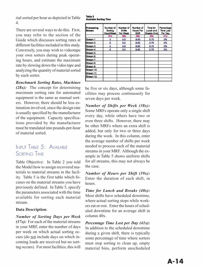
INPUT TABLE 5: AVAILABLE

SORTING TIME

Table Objective: In Table 2 you toldthe Model how to assign recovered ma-terials to material streams in the facil-ity. Table 5 is the first table which fo-cuses on the material streams you havepreviously defined. In Table 5, specifythe parameters associated with the timeavailable for sorting each materialstream.

Data Description:

Number of Sorting Days per Week(37x): For each of the material streamsin your MRF, enter the number of daysper week on which actual sorting oc-curs (do not include days on which in-coming loads are received but no sort-ing occurs). For most facilities, this will

be five or six days, although some fa-cilities may process continuously forseven days per week.

Number of Shifts per Week (38x):Some MRFs operate only a single shiftevery day, while others have two oreven three shifts. However, there maybe other MRFs where an extra shift isadded, but only for two or three daysduring the week. In this column, enterthe average number of shifts per weekneeded to process each of the materialstreams in your MRF. Although the ex-ample in Table 5 shows uniform shiftsfor all streams, this may not always bethe case.

Number of Hours per Shift (39x):Enter the duration of each shift, inhours.

Time for Lunch and Breaks (40x):Most shifts have scheduled downtime,where actual sorting stops while work-ers eat or rest. Enter the hours of sched-uled downtime for an average shift incolumn 40x.

Percentage Time Lost per Day (41x):In addition to the scheduled downtimeduring a given shift, there is typicallysome percentage of time where sortersmust stop sorting to clean up, emptymaterial bins, perform unscheduled

A-15

maintenance, or are otherwise pre-vented from sorting recovered material.Estimate the percentage of each shiftthat is lost due to scheduled and un-scheduled suspensions in sorting.

Helpful Hints: The Model assumesthat all shifts are roughly the same induration and in terms of the responsi-bilities of sorters from one shift to thenext, but this is not always the case. Forexample, the day crew may spend themajority of the time sorting, while thenight crew only sorts for four hours andthen performs other non-sorting dutiesin preparation for the next day. In thiscase, you would have to “define” a shiftas the sum of both day and night shifts,and estimate sorting time, break time,and number of hours for the combinedshift.

Be honest about equipment downtime.To the extent equipment downtime isunderestimated, the Model will assumesorters and automated sorting stationscould be sorting. By underestimatingdowntime, you will also underestimateactual sorting rates.

INPUT TABLE 6: SORTING

CONVEYOR BELT PARAMETERS

Table Objective: In this table, enter rel-evant parameters for analyzing thespeed and capacity of the sorting con-veyor belts in your MRF. MRFs use avariety of ways to move materialstreams through a MRF, but conveyorbelts are by far the most common. Thevolume and weight of material will dic-tate the capacity of each conveyor belt.Capacity, in turn, can be measured bythe depth of material on each conveyorbelt, as that belt moves at a certainspeed. Enter these data points in theappropriate column. Note that densitywill vary over time. If you are sam-pling to estimate density, samples mustbe taken over time to develop an aver-age density.

Data Description:

Conveyor Belt Used for Sorting (43x):For each of the material streams youdefined in Table 2, enter “Yes” for thosethat are being processed via a conveyorbelt.

Different Method Used for Sorting(44x): Indicate “Yes” for each streamwhere some other sorting method isused. For example, material may besorted directly on the floor.

Density Adjustment factor (45a): Insome cases, material does not cover theentire width of the belt (for example,the outer edges may not actually bemoving any material). In this column,enter the percent of the belt width thatactually moves material. If the entirebelt is covered by material ready forsorting, enter 100 percent.

Conveyor Belt Specifications, Width(46x) and Depth (47x): For the con-veyor belt on which each stream is

A-16

sorted, enter the width of the belt(inches) and the average depth of ma-terial (inches) sitting on the belt. Beltwidths can be measured easily. Mate-rial depth should be measured duringoperating hours at the MRF.

Conveyor Belt Specifications, BeltSpeed (48x): Enter the average beltspeed for each of the material streamconveyor belts. You will most likelyhave pre-selected a belt speed for eachof the sorting conveyors at your MRF.The Model will calculate the optimalsorting speed to compare to the actualbelt speeds you enter. Optimal sortingspeed is defined as the minimum beltspeed necessary to move the dailythroughput through the sorting lines ona given day.

Helpful Hints: The conveyor beltwidth and depth drive several impor-tant results, most notably the estimatedmaterial density and optimal conveyorbelt speed for each material stream. Itis important to note that small changesin the conveyor belt width or depth canhave significant impacts on these re-sults, and that you must be as accurateas possible in measuring and estimat-ing these inputs. Since there is high sen-sitivity to changes in these inputs, youmay need to try several inputs to testthe Model’s sensitivity.

Similarly, if you are not sure of the beltspeed, you should measure it. This canbe accomplished simply by measuringa length of the conveyor that is easy tosee, and then timing how long it takes apoint on the belt to move this length.The belt splice could serve as a usefulmeasuring point for measuring beltspeed.

INPUT TABLE 7: BALING

Table Objective: Sorting material isonly part of the function of a MRF.Sorted material will usually be densi-fied prior to shipping. For commingledcontainers (other than glass), and forpaper, baling represents the most effec-tive means of densifying material.Table 7 requires you to enter certain pa-rameters associated with the baling ofeach of the recovered materials at yourMRF.

Data Description:

Is Material Baled (32x): Not all re-covered materials are baled prior to

A-17

shipping. Enter “Yes” only for thoserecovered materials that are baled.

Is Material Sent Straight to Baler(31x): Most recovered materials arestored in temporary storage bins priorto baling. However, in many MRFs themost voluminous material will be sortednegatively off the end of a particularline, and will proceed directly to thebaler throughout the day. Indicate“Yes” for any recovered material thatproceeds directly to a baler.

Bale Size (65x): Enter the average vol-ume of a bale of each of the recoveredmaterials. For best results, you shouldprobably measure the dimensions of 5to 10 bales of each recovered materialtype, and convert your measurementsto cubic yards, and take the average.

Bale Weight (66x): Enter the averageweight of a bale of each of the recov-ered materials.

Baling Time per Bale (64x): Recov-ered materials differ in density, strength,and air space. Use a stopwatch to mea-sure the average time it takes to form acomplete bale of each of the recoveredmaterials at your MRF. Once again,

averaging the baling time for five or tensamples will provide the most accurateresults.

Helpful Hints: Most of these inputscan be determined via real-time mea-surements made at your facility on anormal operating day. However, notethat a larger sample will provide moreaccurate results. That is, measuring ortiming one or two bales will certainlyprovide a ballpark figure. But an aver-age of five, ten, or even twenty baleswill provide a more accurate figure.Since this model helps you to evaluateprocessing on an annual basis, youshould not rely on one measurementmade on a single day of the year, whichcould inadvertently skew the Model re-sults.

INPUT TABLE 8: INCOMING

MATERIAL STORAGE

Table Objective: You will need at leastsome space on your tip floor or in anadjacent storage area to receive incom-ing loads of material. This table helpsyou to estimate the square footageneeded for incoming material undernormal material receiving levels. (Inreality, you will need some overflowspace, since inclement weather andholidays can significantly impact thequantity of incoming materials.)

Data Description:

Number of Days of Storage Required(34x): If you clear your MRF’s tipfloor(s) at the end of each day, youshould enter one day in this column.However, if you store material on thetip floor or in an adjacent storage areafor more than one day, enter the num-ber of days.

A-18

Average Material Depth (35x): Enter,in feet, the average height of the pile ofeach of the incoming streams of mate-rial. You will address the shape of thepile in the next column. Once again,an average of multiple samples is bet-ter than a one-time measurement.

Shape of Pile (unlabeled): Each MRFwill have different storage areas for in-coming material. To most accuratelyestimate the storage space needed forincoming material, you can specify theshape of the storage pile. Enter thenumber below that most closely corre-sponds with the shape of each incom-ing material stream pile:

l Half Cone: Enter 1 for a pile ofmaterial that is stored against asingle wall.

l Quarter Cone: Enter 2 for a pile ofmaterial that is stored in a corner.

l Half Cube: Enter 3 for a pile that isstored in a three-walled bunker.

l Loose: Enter 4 for a pile of mate-rial in the center of the storage area.

l Cube: Enter 5 for material that isstored in a four-walled container orbunker.

Helpful Hints: The issue of incomingmaterial storage is more important forMRFs that are currently in the designstage. If your MRF is operational, youcan estimate the storage requirementssimply by assessing the overflow (orexcess space) on a daily basis. If youare using the Model to analyze opera-tions at an existing MRF, you probablywould use this section to verify yourexisting incoming material storage ca-pacity.

INPUT TABLE 9: BALE STORAGE

Table Objective: You will also needstorage space on the back end of pro-cessing. The Model uses the input onTable 9 to estimate the floor area andvolume needed for storing baled mate-rial prior to shipping.

Data Description:

Material Storage Height (70x): Be-cause bales are cubic, it is easy to esti-mate the volume of material given acertain height. You have already en-tered the average weight and volume of

A-19

a single bale of each recovered mate-rial (Table 7). Enter in column 70x theaverage height off the floor of bales ofeach of the recovered materials.

Number of Days of Storage Required(74x): Shipping a load of recoveredmaterial is dependent upon the sched-ule of haulers and the availability ofmarkets, as well as on having enoughmaterial to make a full load. Therefore,each recovered material may need to bestored inside or on the grounds of yourMRF for some period of time beforeshipping. Enter the average number ofdays needed to store each recoveredmaterial prior to shipping.

Number of Bales in a Load Shipped(72x): You may use several means oftransporting baled material to market.Enter the number of bales in a typicalload of each recovered material.

Helpful Hints: Once again, the issueof storage is often addressed early inthe planning stages of a MRF. If youare using this Model to analyze an ex-isting MRF, the results you generatewill probably only verify the amount ofstorage space you currently have at yourMRF. However, if you are consideringdesigning and building a new MRF, youmay be able to use this section to gainsome insight on the baled material stor-age requirements.

OUTPUT TABLE 1: MATERIALS

RECEIVED

Table Objective: Output Table 1 sum-marizes background information andrecovered material quantities processedat your MRF.

Data Description:

A-20

Miscellaneous (1x through 10): At thetop and to the right of Output Table 1there are several background tables.These background tables summarize thename and location of the MRF, and thepopulation and number of householdsserved by the MRF. Additionally, thesetables show some general MRF oper-ating parameters.

Tons Received (11): Column 11 sum-marizes the total tons of incoming ma-terial that was received at the facility.This is the sum of columns 15x through18x, plus any residues in column 14.

Percent Composition (12): Column 12shows composition of the incoming ma-terial stream.

Material Residue, Tons (14): Based onthe percent residue entered in Column13x, this column shows the estimatedtons of residue produced at the facility.Alternatively, the material residue ton-

nage may be entered as a separate lineitem.

Total Tons Marketed, All Sources (19):This column represents the actualamount of recovered material that ismarketed by your MRF. This columnis calculated by netting out the residues(column 14) from column 11.

Data Source: See Background Table(Columns 1x through 7x, 10x) andTable 1 (Columns 13x, 15x, 16x, and18x)

Helpful Hints: You should verify thetotals in columns 11 and 19, “Tons Re-ceived” and “Tons Marketed,” respec-tively. If the totals shown in the Modeldo not closely or even exactly matchthe data taken from your plant operat-ing reports for Model input, you mayneed to return to Table 1 and verify thatyou have entered annual summary dataaccurately and in the correct columns.

A-21

OUTPUT TABLE 2: ESTABLISHING

PROCESSING STREAMS AND

SORT RATES

Table Objective: Your MRF must pro-cess and sort all of the listed recoveredmaterials. This Output Table shows thequantity of recovered material to besorted, as well as the benchmark sort-ing rate for each material.

Data Description:

Estimated Average Volume per Piece(22): Based on the density of each re-covered material (column 20x) and theaverage weight per piece (column 21x),this column shows the estimated aver-age volume of each piece of sortedmaterial.

Quantity of Material per Year (23):You have already input the quantity ofmaterial to be sorted for one year, mea-sured in tons (column 11). This col-

umn converts material quantities intovolume, based on material density.

Standard Sorting Rate (29): Based onthe average weight per piece (column21x) and on the benchmark sorting rateper hour (column 27 or column 28), thiscolumn estimates the standard sortingrate in terms of the number of piecesthat can be sorted in an hour.

Average Sorting Rate (30): In this col-umn, the average sorting rate (column29) is converted into pieces per second.

Data Sources: See Table 1 (Columns20x and 21x), Table 2 (Columns 24x,25x, 27x, and 28x) and Table 7 (Col-umns 31x and 32x)

OUTPUT TABLE 3: PROCESSING

STREAMS

Table Objective: The first two OutputTables focused on the recovered mate-rials at your MRF. Based on the recov-

A-22

ered material data, the Model aggre-gates each material back into its origi-nal material stream. In this OutputTable, there are really two separatetables analyzing each of the materialstreams (processing streams) at yourMRF. The top table looks at the incom-ing material storage requirements foryour facility, while the bottom tableestablishes certain parameters related tosorting each material stream.

Data Description:

Volume per Sort Stream per Day (33):Based on the total quantity of each re-covered material type, the Model cal-culates the cubic yardage of storagespace needed for each material stream.

Storage Area per Stream (36): Thiscolumn estimates the approximate floorarea needed, based on the number ofdays of storage required before incom-ing material is processed.

Time/Week for Sorting Streams (42):Based on the time parameters in col-umns 37x through 41x, the Model cal-culates the total time available per weekwhen actual sorting of material occurs.

Average Density on Belt Pre-1st Sort(45): This column calculates the den-sity of material on the conveyor belt foreach material stream, prior to sorting.You may wish to verify this density bytaking material samples from the streamduring actual operations.

Belt Speed Req’d to Meet MinimumSorting Requirements (49): This col-umn shows the minimum belt speedrequired to process all incoming mate-rial, given the conveyor belt specifica-tions and the quantity of material to besorted. Note that this output is verysensitive to the belt specifications, andthat small changes to those inputs will

cause significant swings in the mini-mum belt speed.

Data Sources: See Table 8 (Columns34x and 35x), Table 5 (Columns 37x,38x, 39x, 40x, and 41x), and Table 6(Columns 43x, 44x, 46x, 47x and 48x)

Helpful Hints: The primary piece ofuseful information on this table is theminimum conveyor belt speed neededto sort all incoming material. Youshould compare this calculated numberwith the actual belt speed at your facil-ity as a test of current processing effi-ciency.

l If your actual belt speed is muchhigher than the minimum beltspeed, material may be moving toorapidly for sorters to sort at maxi-mum efficiency.

l Conversely, if actual belt speeds arelower than minimum, this suggeststhat you are not keeping pace withincoming material.

OUTPUT TABLE 4: SORTERS AND

SORTING STATIONS

Table Objective: Output Table 4 ana-lyzes the sorting throughput and sorterutilization for each of the recoveredmaterials at your MRF.

Data Description:

Required Sorting Throughput: Weightper Week (50),Weight per Shift-Hour(51), Pieces per Week (52), Pieces perShift-Hour (53), and Volume per Shift-Hour (54): Based on the quantity ofeach recovered material, and theamount of time available over thecourse of a year for processing, thesecolumns display the amount of eachmaterial that must be sorted per hour ofprocessing.

A-23

Number of Sorters/Sorting StationsRequired, Based on Minimum WeightRequirement (55 and 56): These col-umns estimate the minimum number ofsorters or automated sorting stationsneeded to keep pace with incomingmaterial. The calculation is based onthe weight of material to be sorted, andon the benchmark sorting rate fromTable 4, columns 27x and 28x. For re-covered materials that are sorted nega-tively, “-ve sort” is displayed. If thematerial is not sorted, or if it is sentstraight to the baler, these columns willremain blank.

Number of Sorters/Sorting StationsRequired, Based on Belt Speed (57 and58): These columns estimate the mini-mum number of sorters needed, basedon the sorting conveyor belt parametersin Table 6, and on the benchmark sort-ing rates from columns 27x and 28x.

Actual Sort Rate (61): This columncalculates the actual sorting rate basedon the quantity (weight) of material be-ing processed over the course of a fullyear of processing.

Sorter Utilization Rate (62): By com-paring the actual sorting rate in column61 with the benchmark sorting ratesfrom columns 27x and 28x, the Modelestimates the “utilization rate.” Thisrate shows you how busy your sortersand sorting stations are relative to maxi-mum efficiency.

Data Source: See Table 3a (Column59x) and Table 3b (Column 60x).

Helpful Hints: This table is designedto suggest ways to optimize your MRF.An optimized MRF would (theoreti-cally) have the following characteris-tics:

l All sorters would be on or about 100percent utilization (column 62), sig-

A-24

nifying that they spend all of theirtime sorting; and

l The calculated minimum number ofsorters and sorting stations (col-umns 55-58) would be equal to theactual number of sorters and sort-ing stations (column 59x, 60x), sig-nifying that no laborers have anysignificant lulls in productivity onthe sorting line.

You may wish to fine-tune the recov-ered material assignments of each sorterto bring actual processing more in linewith optimized processing.

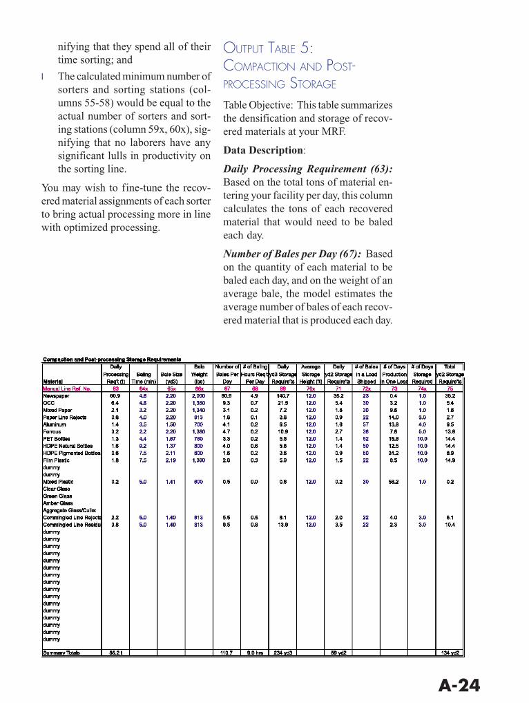
OUTPUT TABLE 5:COMPACTION AND POST-PROCESSING STORAGE

Table Objective: This table summarizesthe densification and storage of recov-ered materials at your MRF.

Data Description:

Daily Processing Requirement (63):Based on the total tons of material en-tering your facility per day, this columncalculates the tons of each recoveredmaterial that would need to be baledeach day.

Number of Bales per Day (67): Basedon the quantity of each material to bebaled each day, and on the weight of anaverage bale, the model estimates theaverage number of bales of each recov-ered material that is produced each day.

A-25

Number of Baling Hours Req’d perDay (68): This column shows theamount of time required to bale eachrecovered material each day.

Daily Volume Storage Requirements(69): Column 69 shows the volume ofbaled material produced each day foreach recovered material.

Daily Floor Area Storage Require-ments (71): In this column the dailyvolume requirement is re-stated in termsof square yardage of floor space.

No. of Days Production in One Load(73): Given the average number ofbales produced per day, and the totalbales that can be accommodated in oneload, this column estimates how manydays of processing is required for eachmaterial to obtain one full load of a re-covered material for shipment.

Total Floor Area Storage Require-ments (75): Because many of the re-covered materials will not be shippedon a daily basis, the Model also esti-mates the total quantity of floor spaceneeded for materials until they areshipped.

Data Source: See Table 7 (Columns64x, 65x, and 66x) and Table 9 (Col-umns 70x, 72x, and 74x)

Helpful Hints: While the output in thistable is done on a material-by-materialbasis, you may be most interested in thetotals at the bottom of the table. Thesetotals let you see, on a plant-wide ba-sis, the time and floor space that mustbe devoted to the baling and storage ofrecovered materials.

As discussed for Tables 7 and 9, thisOutput Table has different uses. If yourfacility is currently operational, youshould use the results in this table toverify the existing time and storage

space requirements. However, if youare planning a new facility, you may usethe results in this table to help in thedesign of the facility, to plan for amplebaler capacity and recovered materialstorage space.

A-26

COSTS: INTRODUCTION

The next four tables in the Model as-sess the costs of operating your MRF.Although the first three tables containboth input and output, they will betreated primarily as input tables. Thelast table in this section of the Modelsummarizes total and unit costs of op-erating your MRF.

In order, the tables in this section ad-dress:

l Capital costs for building and equip-ment

l Labor costs

l Operating and administrative costs(not including labor)

l Total and unit costs (per-ton, percubic yard, per household served)

Helpful Hints: When first opening thespreadsheet and looking at the tables inthis section of the Model, you will see

a range of different line item costs. Forexample, in the Capital Costs section,the Model will show a default list ofcapital cost line items such as “Land andServices,” “Buildings,” “Leasehold Im-provements,” etc. However, if you lookat each of the example tables in thisAppendix, you will see that each of thecost tables has been customized to showline items that are meaningful to theMRF we have used as an example. Asyou progress through the cost sectionof the Model, you may also wish to cus-tomize the expense line items to moreclosely conform to your accounting sys-tem.

INPUT TABLE 1: CAPITAL COSTS

Table Objective: On these two tables,you should enter the capital costs forthe buildings and equipment for yourMRF.

A-27

Data Description:

Capital Costs - Buildings and Land:On the top table, enter the total cost,amortization period, and mortgage ratefor each of the line items in the table.The Model will calculate an averageprincipal and interest payment using themortgage rate and amortization periodyou enter. Note that the resulting an-nual cost is not specific to any year.

Capital Costs - Equipment: For eachof the equipment line items, enter thetotal cost, the year purchased, the lifeexpectancy, amortization period, scrapvalue (if any), and the interest rate.Based on these inputs, the far right col-umn of this table shows the resultingannual cost for each line item.

Unit Cost Summary (81-84; 105-108):At the bottom of each of the two capi-tal cost tables, there are several unit cost

line items. Unit costs are shown on aper-square-foot, per-month and per-tonbasis.

Helpful Hint: The Model treats equip-ment capital costs differently depend-ing on the interest rate that is used. Ifyou plan on borrowing money to fi-nance the purchase of a piece of equip-ment, you should enter a positive inter-est rate. Alternatively, you may wish tosave money over a period of years toreplace old equipment (i.e., capital re-placement). In this case, use a negativeinterest rate. Entering a zero interestrate will cause the Model to use straight-line depreciation.

The capital cost tables at right are notintended to step you through the deci-sion points for capital budgeting at yourMRF. Rather, the annualized costs cal-culated by the table are meant only toapproximate the actual annual expen-diture at your MRF. For this reason, allannualized costs are rounded to thenearest $1,000.

INPUT TABLE 2: LABOR COSTS

Table Objective: On this table, youshould tabulate the supervisory, sortingand non-sorting labor costs (includingbenefits) at your MRF. Additionally,summarize the staffing levels of sort-ing and non-sorting staff.

Data Description:

Labor Costs (109x - 113): On the firstfour lines of the table, enter all regularand overtime earnings for both full-timeand part-time sorters. If possible, de-lineate sorting labor and non-sortinglabor.

Benefits (114x - 123): On these lines,enter the cost of benefits for all labor-ers at the MRF.

A-28

Staff Levels (125x - 129): After enter-ing labor costs, enter the actual numberof employees at your MRF. You shouldseparate sorting and non-sorting labor,as well as supervisory staff.

Unit Cost Summary (130 - 133): Atthe bottom of the table, there are sev-eral unit cost line items. Unit costs areshown on a per-employee, per-monthand per-ton basis.

Helpful Hint: As discussed previously,you may customize the line items on thelabor cost table. In the example at right,total labor costs plus benefits have beenaggregated. You may choose to entercosts in as detailed a manner as suitsyour need.

When entering the staffing levels at thebottom of the table, you may want tocross-reference your responses with thenumber of sorters entered in Table 3a.(Table 3a focuses on only one shift, so

if there a multiple shifts at your MRF,you will have to multiply the total num-ber of sorters in Table 3a with the num-ber of shifts. This should be equal tothe number of sorters entered in line128x in the Labor Cost Table.)

You should NOT enter the cost of anyadministrative staff in this table. Ad-ministrative staff will be tabulated onInput Table 3.

INPUT TABLE 3: OPERATING

AND ADMINISTRATIVE COSTS

Table Objective: On these two tables,enter the operating and administrativecosts associated with your MRF. Op-erating costs include such items as fueland utilities, supplies, repair and main-tenance, and other miscellaneous costs.Administrative costs include both labor(administrative staff) and office-related

A-29

expenses not associated with the actualprocessing of material.

Data Description:

Operating Costs (146x - 174): The left-hand table provides a default list of op-erating cost line items. Enter the ap-propriate amounts, or create your ownline-item labels. In the example at right,all operating costs have been aggregatedinto one line item.

Administrative Staff Earnings (183x- 187): In this section of the secondtable, enter the regular and overtimeearnings of both full and part-time ad-ministrative staff.

Administrative Staff Benefits (188x -196): Enter the cost of benefits for alladministrative staff at your MRF.

Office Expenses (197x - 213): In thissection, enter the office expenses (i.e.,expenses not associated with the pro-cessing of material) at your MRF.

Unit Cost Summary (172 - 174; 214 -216): At the bottom of each table, thereare several unit cost line items. Unitcosts are shown on a per-month and per-ton basis.

OUTPUT TABLE 1: UNIT COST

SUMMARY

Table Objective: This table summarizesthe total costs and unit costs associatedwith your MRF. Additionally, the tablesummarize the total weight and volumeof material received and processed atthe facility.

Data Description:

Material Summary (223-225): The topsection summarizes the weight and vol-ume of material processed per year, aswell as the number of householdsserved by the MRF.

A-30

Capital Cost Summary (226-231):Building and equipment capital costsare shown in total, and also on a per-ton and per-cubic-yard basis.

Operating Cost Summary (232-239):Operating costs, including labor andequipment/maintenance, are shown intotal, as well as on a unit cost basis.Labor costs are delineated by sortersand non-sorters.

Administrative Cost Summary (240-242): Administrative costs are summa-rized at the bottom of the table.

Total Gross Cost Summary (243-254):At the top right of the facing page, totalcapital and operating costs are shownfor your MRF.

Data Source: See Tables 1, 2 and 3.

Helpful Hints: Gross total and unitcosts (as opposed to net) are shown onthis Table. That is, any revenues asso-ciated with the sale of recovered mate-rial or with the receipt of processingfees has not been shown. You may wishto assess material revenues in a sepa-rate spreadsheet (or add a sheet to theModel) to estimate net cost.

A-31

COST ALLOCATION:INTRODUCTION

If you completed the Processing Sec-tion and the Cost Section of the Model,you are prepared to take the final step,and allocate costs to the recovered ma-terials at your MRF. The last section ofthe EPIC MRF Model allows you toallocate costs in several different ways.

There are two pages of tables in thissection. The first page requires you totell the Model how to allocate costs, andis both an input and an output table. Thelast page aggregates the allocated costsinto material groupings. In summary,the cost allocation section contains thefollowing tables:

l Cost allocation by recovered mate-rial (e.g., #1 PET bottles, #2 HDPEnatural bottles, etc.)

l Allocation by material type (e.g.,plastic, glass, metals, etc.)

l Allocation by material stream (e.g.,light fraction line, glass line, etc.)

INPUT/OUTPUT TABLE 1: COST

ALLOCATION BY MATERIAL

Table Objective: On this table, you willallocate the capital, operating and ad-ministrative costs to the individual re-covered materials at your MRF. Afterallocating costs, you can compare therelative cost of processing each recov-ered material.

A-32

Data Description:

Material Allocation Stream (255x):There are ten pre-defined “materialgroups” into which each recoveredmaterial may be classified:

F- Fibers

O1 - Other Miscellaneous

Al - Aluminum

O2 - Other Miscellaneous

Fe - Ferrous

O3 - Other Miscellaneous

Pl - Plastics

O4 - Other Miscellaneous

Gl - Glass

O5 - Other Miscellaneous

In column 255x, enter the appropriateMaterial Group Code from above nextto each recovered material. You havefive miscellaneous material group codesto assign, if needed.

Cost Centers: There are five cost cen-ters, listed across the top of the table:(1) Buildings and Land; (2) EquipmentCapital Cost; (3) Operating Labor; (4)Operating Equipment; and (5) Admin-istration. You can allocate costs foreach cost center independently.

Allocate Costs Automatically (256x,258x, 260x, 262x, 264x): There are twoseparate cells for each cost center youmust fill out to allocate costs automati-cally:

l Input Appropriate Letter: In theappropriate cell, you may allocatecosts in one of three ways: 1) byweight (enter “W” in the appropri-ate cost center); 2) by volume (en-ter “V”); and 3) by unit, or numberof pieces (enter “U”). The Modelwill automatically allocate costsusing the methods you specify.

l Input Amount to Be Allocated: Re-fer to the table at the bottom of thepage. This table lists the total costof each cost center. Enter the ap-propriate dollar amount of the totalcost to be allocated automatically.For example, you may wish to allo-cate all administrative costs auto-matically; in this case, you wouldenter the balance of administrativecosts in this cell.

Allocate Costs By Hand (257, 259, 261,263, 265): In some cases, to get an ac-curate snapshot of the cost of process-ing each material at your MRF, you willpotentially need to allocate some costline items to their appropriate recoveredmaterial by hand. Once again, you willneed to fill out two cells to do so:

l Input Appropriate Letter: If youchoose to allocate costs manually,use the columns labeled “A”, for“Activity.”

l Input Amount to Be Allocated:Once again, refer to the table at thebottom of the page, and enter theappropriate amount from this tableto be allocated by hand. For ex-ample, if you purchase a magnet forsteel and an eddy current separatorfor aluminum, enter the total annu-alized cost of the two pieces ofequipment at the top of the column,and enter the individual annualizedcost of each piece next to the ap-propriate recovered material.

Helpful Hints: While the Model is notdesigned to be a comprehensive activ-ity-based costing (ABC) tool, you cancertainly gain some insight into the rela-tive cost of each different recoveredmaterial.

A-33

l To get a broad brush view of therelative costs of each recoveredmaterial at your MRF, you maywant to allocate all costs automati-cally.

l For a detailed activity-based analy-sis, you can use the manual alloca-tion method.

The flexible design of the Model givesyou multiple options.

OUTPUT TABLE 2: ALLOCATION

BY MATERIAL GROUPINGS

Table Objective: The two tables on thispage utilize the material-by-materialcost allocation table to summarize thecost of different recovered materialgroupings. Each table is described be-low:

Data Description:

Total Costs Allocated by MaterialGroup: In the previous table, you as-signed material group codes to each ofthe recovered materials at your MRF.This table aggregates each materialgroup and shows the total and the totalcost, total tons managed, and the result-ing cost-per-ton. Note that on row272x, you may note what each materialgroup code signifies (in the example atright, material group ‘O1’ has been la-beled “Rejects”).

Total Costs Allocated by ProcessingStreams: Back in the Processing Sec-tion of the Model, you defined indi-vidual material streams at your MRF.This table aggregates material-by-ma-terial costs into each of the materialstreams you defined. Row 276x allowsyou to note what each material streamnumber signifies.

Data Sources: See the previous tablefor material group codes, and Process-ing Section Table 2 (Column 25x) formaterial stream definitions.

Helpful Hints: These tables are use-ful to help you gauge the relative costsof different recovered materials at yourMRF. For example, in the case of aMRF that has separate paper and com-mingled container processing, you mayuse this table to compare the relativecosts of each.

34