mri course textbook
TRANSCRIPT
MRI Physics for Biomedical Researchers
GORDON E. SARTY
University of Saskatchewan
Department of Psychology
9 Campus Drive, Saskatoon, Saskatchewan
Canada S7N 5A5
June 6, 2014

A Course in MRI 2

Contents
1 Overview of the MRI Machinery 9
2 Quantum Mechanics 132.1 Hilbert Space . . . . . . . . . . . . . . . . . . . . . . . . . . . . . . . . . . . . . . . . . 132.2 The Schrodinger and Heisenberg Pictures of Quantum Mechanics . . . . . . . . . . . . . 142.3 Spin in Atomic Nuclei . . . . . . . . . . . . . . . . . . . . . . . . . . . . . . . . . . . . 162.4 The Heisenberg Equations for Spin . . . . . . . . . . . . . . . . . . . . . . . . . . . . . . 192.5 Number of Up and Down Spins in an MRI . . . . . . . . . . . . . . . . . . . . . . . . . . 19
3 Magnetization 213.1 Physically Understanding the Simple Bloch Equation . . . . . . . . . . . . . . . . . . . . 223.2 Mathematically Understanding the Simple Bloch Equation . . . . . . . . . . . . . . . . . 24
4 Radio Frequency (RF) 294.1 The Nature of Light . . . . . . . . . . . . . . . . . . . . . . . . . . . . . . . . . . . . . . 294.2 Decomposition of RF into Circularly Polarized Components . . . . . . . . . . . . . . . . 314.3 The Rotating Frame . . . . . . . . . . . . . . . . . . . . . . . . . . . . . . . . . . . . . . 314.4 The Bloch Equations in the Rotating Frame . . . . . . . . . . . . . . . . . . . . . . . . . 324.5 90o and 180o RF Pulses . . . . . . . . . . . . . . . . . . . . . . . . . . . . . . . . . . . . 334.6 Chemical Shift . . . . . . . . . . . . . . . . . . . . . . . . . . . . . . . . . . . . . . . . 344.7 Inhomogeneities and Magnetic Gradients . . . . . . . . . . . . . . . . . . . . . . . . . . 344.8 Hard and Soft RF Pulses . . . . . . . . . . . . . . . . . . . . . . . . . . . . . . . . . . . 344.9 RF Reception . . . . . . . . . . . . . . . . . . . . . . . . . . . . . . . . . . . . . . . . . 35
5 Slice Selection 395.1 Gradient Fields . . . . . . . . . . . . . . . . . . . . . . . . . . . . . . . . . . . . . . . . 405.2 Slice Selection . . . . . . . . . . . . . . . . . . . . . . . . . . . . . . . . . . . . . . . . 435.3 Slice Profile . . . . . . . . . . . . . . . . . . . . . . . . . . . . . . . . . . . . . . . . . . 435.4 Partial Volume Effect . . . . . . . . . . . . . . . . . . . . . . . . . . . . . . . . . . . . . 44
6 Relaxation 476.1 The Complete Bloch Equation . . . . . . . . . . . . . . . . . . . . . . . . . . . . . . . . 476.2 T ∗2 Decay . . . . . . . . . . . . . . . . . . . . . . . . . . . . . . . . . . . . . . . . . . . 49
7 Pulse Sequences I 537.1 The Spin Echo Sequence . . . . . . . . . . . . . . . . . . . . . . . . . . . . . . . . . . . 547.2 Repeating Basic Sequences . . . . . . . . . . . . . . . . . . . . . . . . . . . . . . . . . . 567.3 Weighting and Image Contrast . . . . . . . . . . . . . . . . . . . . . . . . . . . . . . . . 577.4 Slice Selection in a Pulse Sequence . . . . . . . . . . . . . . . . . . . . . . . . . . . . . . 597.5 Acquiring Signal from Multiple Slices . . . . . . . . . . . . . . . . . . . . . . . . . . . . 607.6 Multiple Echo T2 or Multiple Spin Echo . . . . . . . . . . . . . . . . . . . . . . . . . . . 62
3

A Course in MRI 4
8 K-Space 658.1 Complex Numbers: Magnitude and Phase . . . . . . . . . . . . . . . . . . . . . . . . . . 658.2 Complex Valued Functions . . . . . . . . . . . . . . . . . . . . . . . . . . . . . . . . . . 66
8.2.1 1D real-valued functions . . . . . . . . . . . . . . . . . . . . . . . . . . . . . . . 668.2.2 2D real-valued functions . . . . . . . . . . . . . . . . . . . . . . . . . . . . . . . 678.2.3 1D complex-valued functions . . . . . . . . . . . . . . . . . . . . . . . . . . . . 678.2.4 2D complex valued functions . . . . . . . . . . . . . . . . . . . . . . . . . . . . 68
8.3 Transverse Spin as a Complex Number . . . . . . . . . . . . . . . . . . . . . . . . . . . . 688.4 There is a Transverse Magnetization Complex Number at Every Point in Space in MRI . . 688.5 1D Integral Fourier Transform . . . . . . . . . . . . . . . . . . . . . . . . . . . . . . . . 698.6 2D and 3D Fourier Transforms . . . . . . . . . . . . . . . . . . . . . . . . . . . . . . . . 708.7 Encoding Spatial Information Through Frequency: 1D. . . . . . . . . . . . . . . . . . . . 718.8 The MRI Signal . . . . . . . . . . . . . . . . . . . . . . . . . . . . . . . . . . . . . . . . 748.9 Sampling and Aliasing . . . . . . . . . . . . . . . . . . . . . . . . . . . . . . . . . . . . 778.10 Encoding Spatial Information Through Frequency: 2D . . . . . . . . . . . . . . . . . . . 798.11 Motion Artifact . . . . . . . . . . . . . . . . . . . . . . . . . . . . . . . . . . . . . . . . 838.12 k-Space Heuristics . . . . . . . . . . . . . . . . . . . . . . . . . . . . . . . . . . . . . . 848.13 3D MRI . . . . . . . . . . . . . . . . . . . . . . . . . . . . . . . . . . . . . . . . . . . . 868.14 Advanced k-Space Methods . . . . . . . . . . . . . . . . . . . . . . . . . . . . . . . . . 87
8.14.1 Echo Planar Imaging . . . . . . . . . . . . . . . . . . . . . . . . . . . . . . . . . 878.14.2 Spiral . . . . . . . . . . . . . . . . . . . . . . . . . . . . . . . . . . . . . . . . . 888.14.3 STAR (Single TrAjectory Radial) Acquisition . . . . . . . . . . . . . . . . . . . . 898.14.4 Rosette and Lissajous Imaging . . . . . . . . . . . . . . . . . . . . . . . . . . . . 89
9 Pulse Sequences II 919.1 Inversion Recovery . . . . . . . . . . . . . . . . . . . . . . . . . . . . . . . . . . . . . . 919.2 Turbo Spin Echo: Speeding up the data acquisition . . . . . . . . . . . . . . . . . . . . . 949.3 Using the Steady State to Speed up MRI data acquisition . . . . . . . . . . . . . . . . . . 959.4 FISP Imaging . . . . . . . . . . . . . . . . . . . . . . . . . . . . . . . . . . . . . . . . . 969.5 PSIF Imaging . . . . . . . . . . . . . . . . . . . . . . . . . . . . . . . . . . . . . . . . . 979.6 “True FISP” Imaging . . . . . . . . . . . . . . . . . . . . . . . . . . . . . . . . . . . . . 979.7 FLASH Imaging . . . . . . . . . . . . . . . . . . . . . . . . . . . . . . . . . . . . . . . 989.8 Transient State Imaging . . . . . . . . . . . . . . . . . . . . . . . . . . . . . . . . . . . . 989.9 Using the Ernst Angle . . . . . . . . . . . . . . . . . . . . . . . . . . . . . . . . . . . . . 989.10 Diffusion Imaging . . . . . . . . . . . . . . . . . . . . . . . . . . . . . . . . . . . . . . . 99
10 TRASE Imaging 10510.1 TRASE RF Coils . . . . . . . . . . . . . . . . . . . . . . . . . . . . . . . . . . . . . . . 10510.2 How to use a TRASE NMR signal to reconstruct an image . . . . . . . . . . . . . . . . . 107
10.2.1 k-space origin of a TRASE coil . . . . . . . . . . . . . . . . . . . . . . . . . . . 10710.2.2 TRASE imaging pulse sequences . . . . . . . . . . . . . . . . . . . . . . . . . . 10910.2.3 TRASE slice selection . . . . . . . . . . . . . . . . . . . . . . . . . . . . . . . . 113
11 Image Post Processing: Maps 11511.1 Diffusion Maps . . . . . . . . . . . . . . . . . . . . . . . . . . . . . . . . . . . . . . . . 11511.2 Windowing . . . . . . . . . . . . . . . . . . . . . . . . . . . . . . . . . . . . . . . . . . 11711.3 T1 Maps . . . . . . . . . . . . . . . . . . . . . . . . . . . . . . . . . . . . . . . . . . . . 11811.4 T2 Maps . . . . . . . . . . . . . . . . . . . . . . . . . . . . . . . . . . . . . . . . . . . . 119

5
12 Diffusion Tensor Imaging 12312.1 Diffusion Tensor Weighting . . . . . . . . . . . . . . . . . . . . . . . . . . . . . . . . . . 12412.2 Reducing the Number of Necessary Diffusion Gradient Directions . . . . . . . . . . . . . 12712.3 Elements and Measures of Diffusion Anisotropy . . . . . . . . . . . . . . . . . . . . . . . 12812.4 Other Diffusion Methods . . . . . . . . . . . . . . . . . . . . . . . . . . . . . . . . . . . 129
13 Spectroscopic Imaging 13113.1 From One Spin Isocromat to Many . . . . . . . . . . . . . . . . . . . . . . . . . . . . . . 13213.2 Chemical Shift Artifact in MRI . . . . . . . . . . . . . . . . . . . . . . . . . . . . . . . . 13313.3 Chemical Shift Frequency . . . . . . . . . . . . . . . . . . . . . . . . . . . . . . . . . . 13313.4 J Coupling . . . . . . . . . . . . . . . . . . . . . . . . . . . . . . . . . . . . . . . . . . . 13413.5 The Really Important Molecules . . . . . . . . . . . . . . . . . . . . . . . . . . . . . . . 134
13.5.1 Water (H2O) . . . . . . . . . . . . . . . . . . . . . . . . . . . . . . . . . . . . . 13413.5.2 Lipid (fat) . . . . . . . . . . . . . . . . . . . . . . . . . . . . . . . . . . . . . . . 135
13.6 Suppressing the Water Signal . . . . . . . . . . . . . . . . . . . . . . . . . . . . . . . . . 13513.7 The Other Important Molecules . . . . . . . . . . . . . . . . . . . . . . . . . . . . . . . . 135
13.7.1 Lactate . . . . . . . . . . . . . . . . . . . . . . . . . . . . . . . . . . . . . . . . 13613.7.2 Choline . . . . . . . . . . . . . . . . . . . . . . . . . . . . . . . . . . . . . . . . 13713.7.3 Creatine . . . . . . . . . . . . . . . . . . . . . . . . . . . . . . . . . . . . . . . . 13913.7.4 N-Acetylaspartate (NAA) . . . . . . . . . . . . . . . . . . . . . . . . . . . . . . 140
13.8 Single Voxel Spectroscopy . . . . . . . . . . . . . . . . . . . . . . . . . . . . . . . . . . 14113.9 Spectroscopic Imaging . . . . . . . . . . . . . . . . . . . . . . . . . . . . . . . . . . . . 14313.10Non-Chemical-Shift Spectroscopic Dimensions . . . . . . . . . . . . . . . . . . . . . . . 145
13.10.1 J coupling and the Nuclear Overhauser Effect (nOe) . . . . . . . . . . . . . . . . 14513.11COSY (COrrelation SpectroscopY) . . . . . . . . . . . . . . . . . . . . . . . . . . . . . 147
14 Functional MRI 14914.1 FAIR . . . . . . . . . . . . . . . . . . . . . . . . . . . . . . . . . . . . . . . . . . . . . 15014.2 BOLD . . . . . . . . . . . . . . . . . . . . . . . . . . . . . . . . . . . . . . . . . . . . . 15014.3 Sources of BOLD Signal . . . . . . . . . . . . . . . . . . . . . . . . . . . . . . . . . . . 15314.4 The Hemodynamic Response . . . . . . . . . . . . . . . . . . . . . . . . . . . . . . . . . 154
14.4.1 Neuro-hemodynamic Physiology and the Balloon Model . . . . . . . . . . . . . . 15614.5 Activation Maps and fMRI Experimental Design . . . . . . . . . . . . . . . . . . . . . . 15714.6 Computing and Interpreting Activation Maps . . . . . . . . . . . . . . . . . . . . . . . . 159
14.6.1 The General Linear Model . . . . . . . . . . . . . . . . . . . . . . . . . . . . . . 16114.6.2 BOLDfold . . . . . . . . . . . . . . . . . . . . . . . . . . . . . . . . . . . . . . 161
14.7 More About the Source of the fMRI Signal . . . . . . . . . . . . . . . . . . . . . . . . . 16314.7.1 Neuron Physiology – In Brief . . . . . . . . . . . . . . . . . . . . . . . . . . . . 16314.7.2 The Relationship Between Neural Activity and BOLD . . . . . . . . . . . . . . . 16414.7.3 EEG and MEG . . . . . . . . . . . . . . . . . . . . . . . . . . . . . . . . . . . . 164
15 Flow and Perfusion Imaging 16915.1 Modulus Based Flow Imaging . . . . . . . . . . . . . . . . . . . . . . . . . . . . . . . . 169
15.1.1 Display of angiograms . . . . . . . . . . . . . . . . . . . . . . . . . . . . . . . . 17115.2 Phase-based Flow Imaging . . . . . . . . . . . . . . . . . . . . . . . . . . . . . . . . . . 17115.3 Perfusion . . . . . . . . . . . . . . . . . . . . . . . . . . . . . . . . . . . . . . . . . . . 173
A Math Needed for this Book 177A.1 Vectors . . . . . . . . . . . . . . . . . . . . . . . . . . . . . . . . . . . . . . . . . . . . 177A.2 Inner Products . . . . . . . . . . . . . . . . . . . . . . . . . . . . . . . . . . . . . . . . . 179A.3 Matrices . . . . . . . . . . . . . . . . . . . . . . . . . . . . . . . . . . . . . . . . . . . . 180A.4 Matrix Multiplication . . . . . . . . . . . . . . . . . . . . . . . . . . . . . . . . . . . . . 181

A Course in MRI 6
A.5 Finite Dimensional Operators . . . . . . . . . . . . . . . . . . . . . . . . . . . . . . . . . 181A.6 Cross Products . . . . . . . . . . . . . . . . . . . . . . . . . . . . . . . . . . . . . . . . 182
A.6.1 Determinants . . . . . . . . . . . . . . . . . . . . . . . . . . . . . . . . . . . . . 182A.7 Multiplication of Scalars and Vectors . . . . . . . . . . . . . . . . . . . . . . . . . . . . . 183A.8 Complex Numbers . . . . . . . . . . . . . . . . . . . . . . . . . . . . . . . . . . . . . . 183
A.8.1 Addition of Complex Numbers . . . . . . . . . . . . . . . . . . . . . . . . . . . . 184A.8.2 Multiplication of Complex Numbers . . . . . . . . . . . . . . . . . . . . . . . . . 184
A.9 Complex Vectors and Matrices . . . . . . . . . . . . . . . . . . . . . . . . . . . . . . . . 184
B Statistics Needed for this Book 185
Preface
This small textbook has been used as the basis for a single term graduate level course that I have aimedgenerally at students in the life sciences, particularly psychologists. The material could also be taught ata senior undergraduate level if the students had some background in matrix algebra. The course has beenoffered, beginning in 1999, as an introductory level graduate course in the Division of Bioengineering at theUniversity of Saskatchewan where the Bioengineering students may primarily have either an engineering orbiology background. The mathematics background required to complete the course is elementary for thosewith an engineering background but rather advanced for most life sciences students. To make the course fairand useful to both types of students, one approach that I have used was to assign a major essay requirement– a task that is usually more difficult for the engineers – to complement the quantitative work. Suggestedessays are given in the main text. With that approach, the course has been taught to fit a 12 week term asfollows:Week 1: Quantum Mechanics (Chapter 2)Week 2: Magnetization (Chapter 3)Week 3: RF (Chapter 4)Week 4: Slice Selection and Relaxation (Chapter 5 and 6)Week 5: Pulse Sequences I (Chapter 7)Weeks 6 and 7: k-Space (Chapter 8)Week 8: Pulse Sequences II (Chapter 9)Week 9: Diffusion Weighting and Maps (End of Chapter 9 and Chapter 11)Week 10: Maps, Diffusion Tensors and Spectroscopy (End of Chapter 11, Chapters 12 and 13)Week 11: The Basis of BOLD Contrast (Chapter 14)Week 12: Introduction to fMRI Experimental Design (Chapter 14)
More recently, because of my position in the Psychology department, the course has been aimed pri-marily at students interested in fMRI. In that case I have assigned an fMRI data analysis project, outlinedat the end of Chapter 14, as the term project instead of an essay (and I give an introduction to fMRI at thebeginning of the course). In that case, I cover the material in Chapter 14 first so that student can begin theproject as soon as possible. Thus, depending on how the course is structured, material from this text can beused to teach students from a wide range of backgrounds, from engineering to psychology, have found thecourse useful.
At the end of the book is an appendix on math. The mathematics covered in the appendix representsa raw minimum that I require my students to understand to pass the exams I set. Therefore, not everymathematical topic touched upon in the text is reviewed in the appendix. For example there is no review ofeigenvectors and eigenvalues, nor of differential equations. The students who already have a more advancedmathematical background will get more from the course. But the students with the minimium backgroundcan still understand the necessary physical concepts behind MRI – they will just have fewer points of viewfrom which to think about things.
At the end of the chapters are some suggested exercises. The exercises marked with a star requirebackground math knowledge above the minimum level. Again, it has not been necessary to be able to solvethe starred questions in order to pass the course as I have taught it.
The feedback of all the students who have taken my course is gratefully acknowledged. In particular,Jennifer Hilton needs special thanks because the math appendix was written using her classroom notes.
7

A Course in MRI 8
Thanks are also due to my former lab technician Jennifer Hadley who typed an early draft of the manuscriptand drew many of the figures by computer.
Chapter 1
Overview of the MRI Machinery
When you walk into a clinical or experimental MRI suite, you will generally find three rooms of equipment.One room for the console and operator, one room for the MRI itself and one room for electronics. Theelectronics room is generally behind closed doors and not visible when you walk into the suite.
There typically is a window between the MRI room and the console room so that the operator can seethe person in the MRI. The MRI room itself will be electrically sheilded so that external radio waves cannotenter and ruin the MRI measurement. This sheilding will also be visible as a wire grid in the windowbetween the console and MRI rooms.
It generally takes three computers to run an MRI. One for the operator console, one for running the pulsesequences and one for image reconstruction. Only the console computer is connected to the outside world.The other two computers process data in real time and need to be isolated so that nothing interfers with theirtiming. When a new imaging sequence is written, software must be written for all three computers.
The pulse sequence computer will turn on ampifiers and data receiver channels in the correct orderwith (typically) sub-microsecond accuracy. The amplifiers it controls are the RF amplifier (see Chapter 4)and the gradient amplifiers (see Chapter 8). These amplifiers drive current through the transmitter RF andgradient coils as shown in Figure 1.1. The receiver RF coil picks up the signal from the body being imaged.The received signal passes through an analog-to-digital (ADC) receiver and is stored on the computer priorto image reconstruction.
The heart of the MRI is the main magnetic field. The main field is produced by current flowing inthe main field coils. The main field coils are typically superconducting coils when the filed strength is 1Tesla or greater. A superconducting coil a keep at a temperature that is approximately 4oC above absolutezero (which is −273oC). At that low temperature, the coil has no electrical resistance through a quantummechanical effect in which electrons pair up. Since there is no electrical resistance the coils are chargedwith current once and then the power source is disconnected. The current will then continue to flow virtuallyforever, so the main magnet is always “on”.
To fine tune the main magnetic field, to make it as uniform as possible, the MRI will also contain shimcoils (not shown in Figure 1.1). There will usually be two sets of shim coils, one set is superconducting andthe other set consists of conventional electromagnets. The superconducting shims are adjusted once, whenthe magnet is commissioned while the electromagmet shims are adjusted with each new imaging subject(everyone’s magnetic properties are different!).
MRI is based on the phenomenon of Nuclear Magnetic Resonance (NMR). NMR instruments have beenaround since the late 1940’s but MRI (actually NMRI, Nuclear Magnetic Resonance Imaging) has only beenaround since the early 1980’s. The piece of hardware that sets an NMR instrument apart from an NMRI arethe gradient field coils. Without the gradient field coils, imaging is not possible.
9

A Course in MRI 10
Main field coils(4 total)
��������
X gradient field coils(Two more in front)
�������������������
?
Z gradient coils
6
�������������������
Receiver coil(RF transmitter insimilar location)
�������������9
@@I
-
6
Y
XZ
���
���
���
Y gradient field coils(4 total)
Figure 1.1: The arrangement of magnets in a nuclear magnetic resonance imager.

11
Suggested Essay ProjectsAt the beginning of every course, I assign a project. On possible project is to review the literature and writean essay on one of the following topics:
1. Write a 10 to 15 page review of a recently developed engineering aspect of MRI, e.g. k-space tech-niques, inhomogeneity correction algorithms, motion correction algorithms, RF coil design, the chal-lenges of high field MRI, etc.
2. Write a 10 to 15 page review of a particular biological application of MRI, e.g epilepsy and strokediffusion imaging, measurement of hippocampal volumes, fMRI studies, etc.
If the course is aimed at students whose primary interest in in fMRI then I assign the data analysisproject given at the end of Chapter 14. To get started on an fMRI data analysis project, you will shouldreview some material from Chapter 14 and then learn how to use a data analysis program in parallel withlearning the physics beginning with Chapter 2.

A Course in MRI 12

Chapter 2
Quantum Mechanics
Most introductory books about the physics of magnetic resonance imaging (MRI) written for people inthe life sciences don’t mention quantum mechanics1. This is unfortunate because MRI works through theexploitation of the quantum mechanical spin of the Hydrogen, or other, nuclei. While it is true that abasic working knowledge of MRI can be had by using a heuristic mental image of the magnetization of anatomic nucleus, an appreciation of the nature of that magnetization would then be lost. In addition, a basicknowledge of quantum mechanics is required to understand more complicated nuclear magnetic resonance(NMR) phenomenon (especially on the spectroscopy side). As the science and art of MRI progresses, moreand more of these advanced NMR techniques will be used. The scientist with at least a passing familiaritywith the quantum mechanics of spin will have an advantage over their colleagues when the time comesto apply new techniques to the study of their favorite biological system. So let us begin our study of thephysics of MRI with an introduction to the quantum world.
Quantum mechanics describes the physical world at the scale of atoms and molecules and smaller.Unlike Newtonian mechanics, quantum mechanics does not make definite, deterministic predictions; itonly predicts outcomes in terms of probabilities. But, when large numbers of individual quantum systemsare gathered together, in an ensemble, the behaviour of the ensemble can be predicted determinstically andthe overall behaviour can be described using classical (Newtonian) physical laws.
The basic mathematical objects required for the formulation of quantum mechanics are state vectorsand operators. The vectors are members of a set called Hilbert space and the operators act on or transformthe vectors in the Hilbert space.
2.1 Hilbert SpaceThe mathematical arena of quantum mechanics is Hilbert space. Hilbert space is purely mathematical, itdoesn’t directly represent anything physical, it is only used to compute the probability of a physical event.You can’t travel to Hilbert space except in your mind. Conceptually you can think of Hilbert space asmetaphysical to remove it, in your mind, from physical quantities that can be measured.
Hilbert space is a vector space with definite properties2. The most important property, for us, is the factthat there is an inner product defined on Hilbert space. In complicated quantum mechanical systems, likethe electron orbitals of an atom, the Hilbert space is infinite dimensional; it is a space of functions (i.e. thevectors are functions). Fortunately for us, spin systems, like the spin of the Hydrogen nucleus, are describedvia finite dimensional Hilbert spaces.
1Quantum mechanics is now over 100 years old. The birth of quantum mechanics occured when Max Planck announced hissolution to the “ultraviolet catastrophe” in a talk to the German Physical Society in Berlin on December 14, 1900. Until then, no onehad been able to come up with an explanation of observed black body radiation; classical physics predicted infinite amplitude at higherfrequencies – a catastrophe. Planck solved the problem with the introduction of the famous equation E = hν.
2Explicitly, a Hilbert space is an inner product vector space that is complete; all convergent sequences in the Hilbert space convergeto an element of the Hilbert space. See the slim volume by P.R. Halmos [9] for a nice mathematical introduction to Hilbert space.
13

A Course in MRI 14
A finite dimensional Hilbert space is just an ordinary (complex) vector space made up of n-tuples ofnumbers from C, the set of complex numbers, and is denoted by Cn where n is the dimension of the vectorspace. For the spin of a Hydrogen nucleus, n = 2. So C2 is the Hilbert space relevant to MRI. This is assimple as quantum mechanics gets!
Let’s explore the nature of the inner product concretely in C2. A 2-tuple in C2 is written as a columnvector:
a =
(a1
a2
)=
(a1R + ia1I
a2R + ia2I
)The components of the vector, a1 and a2, are complex numbers with real and imaginary parts. The real partof component a1 is a1R and the imaginary part is a1I and can be identified by the preceding i =
√−1. The
inner product on C2 (or any Hilbert space) is written as 〈a | b〉 = aT b, where the T stands for transpose,and is computed as
〈a | b〉 = aT b =(a1 a2
)( b1b2
)= (a1R + ia1I)(b1R − ib1I) + (a2R + ia2I)(b2R − ib2I)= (a1Rb1R + a1Ib1I + a2Rb2R + a2Ib2I) + i(a1Ib1R − a1Rb1I + a2Ib2R − a2Rb2I).
In computing the inner product the relation i2 = −1 is used. Also note that the bar over the components ofb denotes complex conjugation; an operation that changes the +i to −i in a complex number.
The inner product 〈a | a〉 = ‖a‖2 is the square of the norm or length of the vector a. The complexconjugation in the definition of the inner product guarantees that the inner product of a vector with itselfwill be a real number; there will be no imaginary part in the result. Therefore it makes sense to talk aboutthe length of a vector and distance in Hilbert space. The inner product, via the norm, gives a metric on theHilbert space3.
Let’s return now from C2 to the discussion about generic Hilbert spaces. Denote a general Hilbert spacewith H and a generic vector as ψ, so ψ ∈ H in terms of sets. The final Hilbert space objects we need toconsider are operators. A generic operator G is a “bounded linear transformation on H”. G maps a vectorψ to another vector φ in a linear way4. We write
G : ψ 7→ φ or G(ψ) = φ.
The set of all operators onH is denoted by L(H).In finite dimesional Hilbert spaces, operators are given by matrices; in the case of C2 the operators are
2×2 matrices with complex entries. In infinite dimensions, operators can be thought of as matrices but onehas to restrict the values of the matrix entries so that the resulting operator is “bounded” 5.
2.2 The Schrodinger and Heisenberg Pictures of Quantum Mechan-ics
We now will relate the vectors ψ ∈ H and the operators G ∈ L(H) to physical quantities.Vectors ψ represent the state of a quantum mechanical system. Operators G are associated with a
physical observable g. For example, the energy of a quantum mechanical system E is represented by theHamiltonian operator H 6.
The expectation value of an observable g is denoted by 〈g〉 or 〈G〉 and is calculated from
〈G〉 = 〈ψ | Gψ〉3In the terms of advanced mathematical analysis, a Hilbert space is a metric space.4A linear transformation G is one that satisfies G(cψ + dφ) = cG(ψ) + dG(φ) where c, d ∈ C are scalars.5A bounded operator is one that satisfies ‖Gψ‖ < k‖ψ‖ for some fixed real number k ∈ R and for all ψ ∈ H.6Ideally, to maintain consistent notation, we would represent energy by h but the historical precedent is to use E instead of h.
15
In other words, if you know that a quantum mechanical system is in the state ψ and you wanted to knowwhat the result of a measurement of the physical quantity g would be, the rules of quantum measurementtheory tells you that, on average, the value of g will be 〈ψ | Gψ〉. Quantum mechanics will not give aprecise, definite answer.
The state ψ represents the set of all possible outcomes of a measurement and has information aboutthe probabilities of the outcomes (i.e. some outcomes will be more probable than others). The vector ψrepresents unrealized possibilities. A possibility is selected, or realized, when a measurement is taken.
Quantum mechanics makes precise predictions about how the expectation value of a measurable quan-tity evolves in time when it is not being measured. This process can be described by assuming that thestate ψ evolves in time - the Schrodinger picture - or by assuming that the operator G evolves in time - theHeisenberg picture. Quantum mechanics from Schrodinger’s point of view is known as “wave mechanics”;quantum mechanics from Heisenberg’s point of view is known as “matrix mechanics”7. In either case,quantum mechanics describes the evolution of unrealized possibilities. The evolution in interrupted wheng is measured because the unrealized possibilities then become a realized quantity8. The evolution can alsobe started by a preparation, which, in the language of the Schrodinger picture, forces the system into a welldefined state ψ(0).
The process of putting a sample or patient into the strong magnetic field of an MRI prepares the quantummechanical spin system of interest – the spins of the Hydrogen nuclei.
The evolution of a quantum mechanical system is described via the Hamiltonian, H . In fact the defini-tion of the Hamiltonian completely defines the quantum mechanical system. Once the energy configurationof the system is defined, everything is defined. Everything in physics can be considered as some aspect ofenergy9!
In the Schrodringer picture the state ψ evolves according to the Schrodringer equation:
Hψ(t) = i~d
dtψ(t) (2.1)
where ~ = 1.05457266 × 10⁻³⁴ J·s (Joule seconds) is h/2π where h is Planck’s constant10. The solutionto Schrodringer’s equation11 is
ψ(t) = exp
(− it~H
)ψ(0). (2.2)
In the Heisenberg picture, the operator G evolves according to the Heisenberg equation:
d
dtG(t) =
i
~[H,G(t)] (2.3)
where [·, ·] is the commutator defined by
[H,G(t)] = H G(t)−G(t)H
Note that the commutator is not in general equal to zero because operators, or matrices, do not in generalcommute; that is for operators A and B it will generally (but not always!) be true that AB 6= BA. Thesolution to Heisenberg’s equation is given by
G(t) = exp
(it
~H
)G(0) exp
(− it~H
). (2.4)
7Heisenberg came up with his approach first, in 1925. Schrodinger followed with his method in 1926 and it was soon realized thatthe two approaches were mathematically equivalent.
8It is a philosophical point of contention among physicists about when a measurement can be said to have occurred. In thelaboratory it is quite clear that a measurement has occurred when a number is obtained. But it is not so clear when the “measurementprocess” can be said to have occured in general. Some, like Roger Penrose [16, 17], believe that new physics are required to solve theproblem and that such new physics may even shed some light on the mystery of our consciousness!
9It appears possible that information instead of energy can be used to give a mathematical description of physics, but informationmodels of physics aren’t as widely taught as energy models.
10In the limit as h→ 0 the predictions of quantum theory match the predictions of classical or Newtonian theory.11The exponential of an operatorG is given by the Taylor series exp(G) = I+(1/2!)G2 +(1/3!)G3 + . . . where I is the identity
operator or, in finite dimensional Hibert space, the identity matrix.

A Course in MRI 16
Using Equations (2.2) and (2.4), it can be shown that
〈ψ(0) | G(t)ψ(0)〉 = 〈ψ(t) | G(0)ψ(t)〉.
The left side is a Heisenberg picture calculation, the right side is a Schrodinger picture calculation. The twopictures are physically equivalent in that they predict the same expectation value for physical observables.
2.3 Spin in Atomic NucleiAs a physical particle, the atomic nucleus is modeled in quantum mechanics as a mere point in space12.Since the point is without diameter, it makes no sense to talk about its angular momentum. And yet, whenthe nucleus is placed within a magnetic field, it behaves as if it had some angular momentum. This intrinsicangular momentum is called spin 13. This quantum mechanical spin is described by a set of spin operators14:
~I = (Ix, Iy, Iz)
These operators are finite dimensional, represented by finite matrices that act on vectors in Cn. Thespin operators satisfy the following commutation relations:
[Ix, Iy] = iIz
[Iy, Iz] = iIx (2.5)[Iz, Ix] = iIy
(Recall that [Ix, Iy] = IxIy − IyIx, etc..)The dimension of Cn is determined by the spin quantum number I , which is a “half-interger”; that is
I ∈ {0, 12 , 1,
32 , 2, . . .}. The dimension of the relevant Hilbert space is given by n = 2I + 1. The nucleus
of a Hydrogen atom, a proton, has “spin 1/2”; that is I = 1/2. Therefore n = 2 · 12 + 1 = 2 so the Hilbert
space is C2 and Ix, Iy and Iz are 2× 2 matrices for the proton.Solving the communtation relations (2.5) for n = 2 gives:
Ix =1
2
[0 11 0
], Iy =
1
2
[0 −ii 0
], Iz =
1
2
[1 00 −1
](2.6)
Mathematically the commutation relations can be shown to be related to rotations (spinning) but show-ing that would require the introduction of the mathematical objects of Lie algebras and groups15. So we’llskip that derivation and simply accept the commutation relations as given.
The all-important Hamiltonian of an intrinsic spin system is given by
H = −γ~ ~B · ~I
where ~B is a magnetic field16. If ~B = B0~k as in the main magnetic field of an MRI,
H = −γ~B0 · Iz12Actually, in string theory the nucleus is modeled as more than a point. But knowlwdge of string theory is definitely not required
to understand MRI! See B. Greene’s book [6] for a non-mathematical description of string theory.13The phenomenon of spin can be shown to arise from the consideration of the laws of special relativity at the atomic, quantum,
level.14 Most physics texts define ~J = ~~I as the vector of spin operators because it is more directly related to angular momentum. Thanks
to my student Somaie Salajeghe for pointing that out to me.15This works by considering spin operators to be representations of the spin group SU(2) which can be shown to be a “double
cover” of the rotation group SO(3). SU(2) and SO(3) are examples of Lie groups which are a set of mathematical objects with amultiplication operation of some sort along with some kind of geometry. The multiplication rules of groups define symmetries. Thephysical laws that we know about are the way they are because of their symmetries. From symmetries given by Lie groups, one canderive laws of motion from the related Lie algebras. An algebra is another kind of mathematical set with its own rules of multiplication.Multiplication in Lie algebras is given by the commutator brackets [·, ·]. Equations (2.5) define the Lie algebra su(2) which can begenerated from the Lie group SU(2) through a process that involves the exponentiation of the Lie group objects (which are matriceshere).
16Or H = −γ ~B · ~J , see footnote 14.

17
(γ is the gyromagnetic ratio; more about that below). This Hamiltonian describes the energy of the spinsystem.
Let’s back-up now to get a more concrete idea of what the spin operators ~I are all about.The fundamental physical quantity of concern to us in the study of MRI is the magnetic moment associ-
ated with the intrinsic spin of the nucleus. We can visualize the magnetic moment of a nucleus by imagingthe nucleus to be a finite-size ball instead of just a point. It is important to rememeber that attempting todo classical Newtonian-type calculations with a finite size nucleus will lead to wrong answers17. But theformulation of a quantum theory can be done by analogy with the classical (Newtonian) theory. Specificallythe procedure is to set up a corresponance between the classical, actually measurable, physical quantity, gand its operator 〈G〉.
Here, for spin, we need to set up a corresponance between the classical magnetic moment ~µ and theoperators for magnetic moment ~U .
So, first note that our spinning nucleus ball is charged, it has a charge of +1 as you will recall frombasic physics or chemistry. In our imagination we could think of something like the spinning ball shown inFigure 2.1.
Figure 2.1: Spinning charged ball model of the nucleus.
Current is defined as moving charge and that is exactly what we have on the surface of our ball nucleus.If you integrate all the moving charges you get an equivalent current loop. A current loop is a well-defined current flowing in a well-defined circle in space. If that circle encloses an area of A we have in ourimagination a picture that looks like Figure 2.2.
Figure 2.2: The nuclear current in an abstract representation.
In Figure 2.2 j is the total effective current generated by the spinning, charged, nucleus. The magneticmoment associated with any current loop is defined by a vector ~µ whose length is ‖~µ‖ = jA and directionis perpendicular to the current loop in the direction given by the right hand rule18, so we can add magneticmoment to our abstract picture of the atomic nucleus as shown in Figure 2.3. It is this magnetic moment
17With a given spin, s, charge, q, and mass, m, classical physics predicts that γ = sq/mc for a finite-size ball nucleus where c isthe speed of light. But that answer is wrong by a factor of 2! So the quantum mechanical spin of a nucleus must be regarded as anintrinsic property of the nucleus. In reality γ = gsq/mc where g is the “nuclear g factor” that has a value of approximately 2. Theexact value of g actually depends on the number of different types of particles the universe contains; so the measurement of g can beused to test theories of physics [26]! For practical calculations we take g = 2 so for the proton s = 1
2, γ = q/mc where m and q are
the mass and charge of the proton respectively18The magnetic moment is a short-hand way of representing the magnetic field associated with the current loop.

A Course in MRI 18
vector that people are implicitly talking about when they describe a nuclear spin as being like a “little barmagnet”.
~µ
Figure 2.3: Magnetic moment added using the right hand rule. With the right hand rule, curl the fingers ofyour right hand in the direction of the current j, then your thumb will point in the direction of ~µ.
We will have more to say about ~µ in Chapter 3 but for now we note that classical electrodynamics tellsus that the energy of a magnetic moment19 in a magnetic field is
E = −~µ · ~B. (2.7)
The operator ~U associated with the classical ~µ is~U = γ~~I.
(This is the simplest definition for the units of measurement to work out. We could also use ~J as defined infootnote 14 to get ~U = γ ~J which fits better with the units of measurement and which more clearly shows γas the ratio of magnetic moment to angular momentum; see also Equation (3.10) in Chapter 3.)
The classical energy E is associated with the Hamiltonian operator so
H = −~U · ~B = −γ~~I · ~B
as we had before.One final important point about quantum mechanics: physical quantities can only take on discrete val-
ues: physics is quantized. The allowed discrete values for a physical quantity are given by the eigenvaluesof the associated operator. In particular, the eigenvalues of the Hamiltonian give the allowed energy levelsfor the quantum system.
For the spin Hamiltonian H = −γ~ ~B · ~I , the eigenvalues, or allowed energy levels, are given by:
Em = −γ~B0m
where m ∈ {−I, I + 1, . . . , I − 1, I}.So for protons, where I = 1/2, m ∈ {−1
2 ,12}. Only 2 energy states are allowed, one “going with the
magnetic field” or “spin up” and one “going against the magnetic field” or “spin down”. To define the upand down proton spins more specifically, take the magnetic field to be in the z direction (along the bore ofa clinical MRI) so that ~B = (0, 0, B0). Then H = −γ~B0Iz with energy levels Eup = E− 1
2= γ~B0/2
and Edown = E 12
= −γ~B0/2. These energy levels (divided by −γ~B0) are the eigenvalues of the twoeigenvectors20 of the 2×2 Iz matrix given by
ψup =|↑〉 =
[10
]and ψdown =|↓〉 =
[01
]. (2.8)
19It takes energy to move the magnetic moment in a magnetic field because the magnetic field of the current loop will attract orrepel the external magnetic field.
20These eigenvectors are “normalized” meaning that they are scaled so that their length is 1. In general, if some vector ~v is aneigenvalue of a matrix A, that is if A~v = m~v where m is an eigenvalue, then any multiple c~v of that vector is also an eigenvector.Prove that by multiplying both sides of A~v = m~v by c. In quantum mechanics, only state vectors of length 1 have any meaningbecause of their ultimate relationship to probability which must have values between 0 and 1.
19
These are the up and down states of the proton spin as represented in the abstract Hilbert space of states C2.
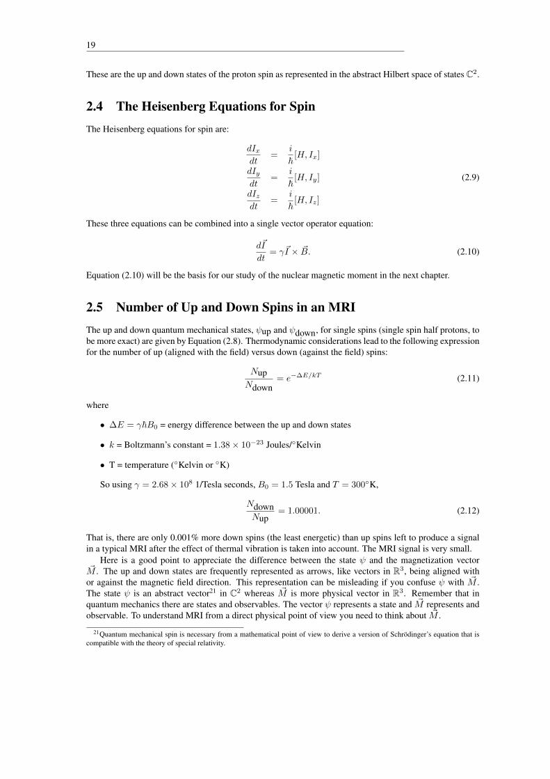
2.4 The Heisenberg Equations for SpinThe Heisenberg equations for spin are:
dIxdt
=i
~[H, Ix]
dIydt
=i
~[H, Iy] (2.9)
dIzdt
=i
~[H, Iz]
These three equations can be combined into a single vector operator equation:
d~I
dt= γ~I × ~B. (2.10)
Equation (2.10) will be the basis for our study of the nuclear magnetic moment in the next chapter.
2.5 Number of Up and Down Spins in an MRIThe up and down quantum mechanical states, ψup and ψdown, for single spins (single spin half protons, tobe more exact) are given by Equation (2.8). Thermodynamic considerations lead to the following expressionfor the number of up (aligned with the field) versus down (against the field) spins:
NupNdown
= e−∆E/kT (2.11)
where
• ∆E = γ~B0 = energy difference between the up and down states
• k = Boltzmann’s constant = 1.38× 10⁻²³ Joules/◦Kelvin
• T = temperature (◦Kelvin or ◦K)
So using γ = 2.68× 10⁸ 1/Tesla seconds, B0 = 1.5 Tesla and T = 300◦K,
NdownNup
= 1.00001. (2.12)
That is, there are only 0.001% more down spins (the least energetic) than up spins left to produce a signalin a typical MRI after the effect of thermal vibration is taken into account. The MRI signal is very small.
Here is a good point to appreciate the difference between the state ψ and the magnetization vector~M . The up and down states are frequently represented as arrows, like vectors in R3, being aligned with
or against the magnetic field direction. This representation can be misleading if you confuse ψ with ~M .The state ψ is an abstract vector21 in C2 whereas ~M is more physical vector in R3. Remember that inquantum mechanics there are states and observables. The vector ψ represents a state and ~M represents andobservable. To understand MRI from a direct physical point of view you need to think about ~M .
21Quantum mechanical spin is necessary from a mathematical point of view to derive a version of Schrodinger’s equation that iscompatible with the theory of special relativity.

A Course in MRI 20
Exercises1. Compute the inner product of
a =
(5 + i67 + i8
)and b =
(1 + i52 + i4
)Also compute 〈a | a〉 and 〈b | b〉.
2. *By differentiating Equation (2.2), show that it is a solution to Schrodinger’s Equation (2.1).
3. *By differentiating Equation (2.4), show that it is a solution to Heisenberg’s Equation (2.3). Hintfor this and the previous exercise: (d/dt) exp(ctG) = cG exp(ctG) = c exp(ctG)G where c is anarbitrary complex number and G is an arbitrary operator.
4. *Using Equations (2.2) and (2.4), show that
〈ψ(0) | G(t)ψ(0)〉 = 〈ψ(t) | G(0)ψ(t)〉
5. Show that the matrices of Equation (2.6) satisfy the commutation relations (2.5).
6. Using Equation (2.7), compute the energy of a magnetic moment in the magnetic field ~B = B0~k for
the following orientations of ~µ:
(a) ~µ = µ0~k (aligned with the magnetic field)
(b) ~µ =√
2µ0(~ı+ ~k)
(c) ~µ = µ0~ı (perpendicular to the magnetic field)
(d) ~µ =√
2µ0(~ı− ~k)
(e) ~µ = −µ0~k (aligned against the magnetic field)
Which orientation has the least energy? Which orientation has the most energy?
7. *With ~B = Bz~k show that the Heisenberg Equations (2.9) for spin are equivalent to the vectoroperator Equation (2.10). Hint: UseH = −γ~ ~B·~I , the commutation relations (2.5) and the definitionof the cross product as given by the determinant
~A× ~B =
∣∣∣∣∣∣~i ~j ~kAx Ay AzBx By Bz
∣∣∣∣∣∣ .

Chapter 3
Magnetization
Section 2.4 concluded with a Heisenberg vector (operator) equation for the evolution of spin operators.Specifically:
d~I
dt= γ~I × ~B. (3.1)
We are interested in the evolution of the expectation value of the magnetic moment or, as it is more com-monly known, the magnetization.
Recall that ~U = γ~~I . So the Heisenberg equation for the magnetic moment is obtained by multiplyingboth sides of Equation (3.1) by γ~ which gives
d~U
dt= γ~U × ~B. (3.2)
The magnetization is 〈~µ〉 = 〈ψ | ~Uψ〉 whenever the state of the system is ψ. So to obtain an equation forthe magnetization, first let Equation (3.2) act on ψ:
d~U
dtψ = (γ~U × ~B)ψ. (3.3)
ord
dt~Uψ = γ~Uψ × ~B. (3.4)
Now form the inner product of Equation (3.4) with ψ:
〈ψ | ddt~Uψ〉 = 〈ψ | γ~Uψ × ~B〉. (3.5)
ord
dt〈ψ | ~Uψ〉 = γ〈ψ | ~Uψ〉 × ~B. (3.6)
ord〈~µ〉dt
= γ〈~µ〉 × ~B. (3.7)
So, if we let ~M = 〈~µ〉 where ~M represents the behavior of an ensemble of nuclear spins, then we have
d ~M
dt= γ ~M × ~B. (3.8)
This is Bloch’s Equation without relaxation terms. Many introductory texts on MRI begin with Equation(3.8) but now you have an idea of where Bloch’s Equation really comes from!
We will spend the rest of the chapter understanding the solution of the simple Bloch equation.
21

A Course in MRI 22
3.1 Physically Understanding the Simple Bloch EquationVisualize, now, the ensemble of nuclear spins as a magnetic moment as shown in Figure 3.1.
������������������������
������������������������
����
A
~M
i
or
z
y
x
~M
Figure 3.1: Our familiar abstraction of the magnetic moment of a single atomic nucleus carries over anensemble of nuclei (left). The ensemble magnetic moment M consisting of the sum of the individualmagnetic moments is equivalent to some current i enclosing some area A. We can further abstract ourrepresentation of the ensemble magnetic moment to just the vector ~M (right).
If the magnetization ~M is placed in a magnetic field ~B, it experiences a torque1 ~T :
~T = ~M × ~B. (3.9)
Recall that the cross product of two vectors ~A and ~B is a vector that is perpendicular to ~A and ~B in adirection given by the “right hand rule”2 as illustrated in Figure 3.2.
~AX ~B (out of page)
~B
~A ~A
~AX ~B (into page)
~B
Figure 3.2: The geometrical relationship between ~A, ~B and ~A and ~B. The vectors ~A and ~B define a planeand ~A and ~B is perpendicular to that plane.
So, if ~B is a magnetic field in the z direction and we tried to move ~M away from the z direction alongthe z–y plane, the result is a torque vector along the x direction as shown in Figure 3.3.
The torque generated by moving ~M away from ~B is trying to force ~M back to alignment with ~B. When~M is finally aligned with ~B there will be no torque since the cross product of parallel vectors is zero.
The ensemble of spinning nuclei also has mass and therefore a collective value (expectation value) ofangular momentum ~J . The angular momentum ~J is related to ~M by the gyromagnetic ratio γ:
~M = γ ~J. (3.10)1Note that, quantum mechanically, the magnetic moment does not even exist until the nucleus is placed in a magnetic field. Placing
the nucleus in the magnetic field causes a Zeeman spliting of the overall energy levels of the nucleus. The new energy levels, bythemselves, are described by the quantum mechanics of spin outlined in Chapter 2.
2Take a pen and, on your right hand, write ~A on your thumb, ~B on your pointing finger and ~A × ~B on your middle finger. Thenyou will be able to align your fingers with the drawings in Figure 3.2.

23
x
y
z
~T
~B
~M
implied twist on ~M
Figure 3.3: Geometrical representation of ~T = ~M × ~B. Representing a torque with a vector means that thetwist of the torque is given by the right hand rule, this time with the thumb pointing with the torque vectorT and the fingers curling in the direction of the implied twist.
For hydrogen nuclei:
γ = 2.68× 10⁸ T−1s−1
or, in, perhaps, more familiar terms:
γ
2π= 42.7 MHz/T
where the unit T is the Tesla, a measure of magnetic field strength and MHz is MegaHertz or one millioncycles per second.
The angular momentum aspect of ~M makes the system dynamic. Now when you knock the magne-tization away from the main magnetic field, the gyroscopic forces caused by the angular momentum willprevent the magnetization from quietly returning to alignment with the magnetic field. Instead, the magne-tization will precess around the magnetic field as shown in Figure 3.4.
x
y
z
~B ~M
Figure 3.4: The magnetization vector ~M precesses around the magnetic field ~B.

A Course in MRI 24
The change in angular momentum associated with torque is3
d ~J
dt= ~T . (3.11)
Since ~J = 1γ~M and ~T = ~M × ~B,
d ~J
dt=
d
dt
(1
γ~M
)= ~M × ~B
ord ~M
dt= γ ~M × ~B
which is Bloch’s equation.
3.2 Mathematically Understanding the Simple Bloch EquationLet’s simplify the Bloch equation by setting
~B = B0~K
so thatd ~M
dt= γ ~M × ~B
becomesd
dt(Mx~ı+My~+Mz
~k) = γ(Mx~ı+My~+Mz~k)×B0
~k.
Using the determinant as a computational aid (see Appendix A) the cross product is:
~M × ~B =
∣∣∣∣∣∣~ı ~ ~kMx My Mz
0 0 B0
∣∣∣∣∣∣ = MyB0 ~ı−MxB0 ~
sod
dt(Mx ~ı+My ~+Mz
~k) = γMyB0 ~ı− γMxB0 ~
or in component form, equating the~ı term on the left side with~ı term on the right side, the left ~ term withright ~ term and the left ~k term with right ~k term:
dMx
dt= γB0My
dMy
dt= −γB0Mx
dMz
dt= 0
The component equations have the solution
Mx(t) = Mx(0) cos(ω0t)−My(0) sin(ω0t)
My(t) = Mx(0) sin(ω0t) +My(0) cos(ω0t) (3.12)Mz(t) = Mz(0)
3This is the rotational equivalent of Newton’s third law, m~a = ~F or ddtm~v = ~F which says the rate of change of momentum is
equal to the force. The torque equation says that the rate of change of angular momentum is equal to torque.

25
where
~M(0) = Mx(0)~ı+My(0)~+Mz(0)~k
is the initial value of the magnetization at time t = 0, and ω0 = −γB0.What does this solution mean?First, the z component, Mz , does not change; it stays at Mz(0) forever. What about the x and y com-
ponents? To simplify the view, assume, without loss of generality4, that My(0) = 0. With this simplifyingassumption the initial magnetization vector ~M(0) is as shown in Figure 3.5.
x
y
z
Mx(0)
~M(0)
Mz(0)
or viewed from the top:
x
y
Mx(0)
Figure 3.5: The initial magnetization ~M(0) when My(0) = 0.
4This just amounts to rotating the x,y,z frame about the z-axis so that the intital magnetization vector ~M is lined up with the xaxis. In doing that rotation, we do not change any physics, just the artificial, mathematical, way of labeling spatial directions.

A Course in MRI 26
The solution of the Bloch equations is simplified to:
Mx(t) = Mx(0) cosω0t = Mx(0) cos[−γB0t]
My(t) = Mx(0) sinω0t = Mx(0) sin[−γB0t] (3.13)
with Mz staying constant. Let’s look at the solution given by Equations (3.13) at times t where:
t ∈{
0,− π
4ω0,− π
2ω0,− 3π
4ω0,− π
ω0,− 5π
4ω0,− 3π
2ω0,− 7π
4ω0,−2π
ω0
}or
−ω0t ∈{
0,π
4,π
2,
3π
4, π,
5π
4,
3π
2,
7π
4, 2π
}Note that ω0 is a negative number so that all the times t above are positive numbers. The Bloch equationsolutions are:
Mx(0) = Mx(0)My(0) = 0
Mx(− π4ω0
) = 1√2Mx(0)
My(− π4ω0
) = − 1√2Mx(0)
Mx(− π2ω0
) = 0
My(− π2ω0
) = −Mx(0)
Mx(− 3π4ω0
) = − 1√2Mx(0)
My(− 3π4ω0
) = − 1√2Mx(0)
Mx(− πω0
) = −Mx(0)
My(− πω0
) = 0
Mx(− 5π4ω0
) = − 1√2Mx(0)
My(− 5π4ω0
) = 1√2Mx(0)
Mx(− 3π2ω0
) = 0
My(− 3π2ω0
) = Mx(0)
Mx(− 7π4ω0
) = 1√2Mx(0)
My(− 7π4ω0
) = 1√2Mx(0)
Mx(− 2πω0
) = Mx(0)
My(− 2πω0
) = 0
Graphically these solutions at the nine selected times are represented by the cartoons shown in Figure 3.6.The x–y component of the magnetization is rotating about the z-axis while the z component stays
constant. That is, the magnetization ~M is precessing about the z-axis. Note that, because of the minus signin ω0, the precession is in the clockwise direction.5
The frequency of the precession is ω0 = −γB0. This is the Larmor frequency. It depends on thestrength of the magnetic fieldB0. The units of ω0 are radians/second. A more convenient unit for frequencyis η = ω
2π which has units of cycles/second or Hertz. So, in Hertz, the Larmor frequency is
η0 = − γ
2πB0
which for Hydrogen nuclei is
η0 = −42.7
(MHz
T
)×B0(T)
and for a 1.5 T magnet
|η0| = 42.7MHz
T× 1.5 T = 64 MHz.
5In math, positive rotation is counterclockwise in the usual right-handed x–y coordinate system.

27
x
y
Mx = Mx(0)
t = 0
x
y
−Mx(0)√2
Mx(0)√2
t = − π4ω0
x
y
t = − π2ω0
My = −Mx(0)
x
y
t = − 3π4ω0
My = −Mx(0)√2
Mx = −Mx(0)√2
x
y
t = − πω0
Mx = −Mx(0)
x
y
t = − 5π4ω0
Mx = −Mx(0)√2
My = Mx(0)√2
x
y
t = − 3π2ω0
My = Mx(0)
x
y
t = − 7π4ω0
Mx = Mx(0)√2
My = Mx(0)√2
x
y
t = − 2πω0
Mx = Mx(0)
Figure 3.6: Plugging in a few specific time points into the solution to the Bloch equation given by Equations3.13 reveals a precessing magnetization vector.

A Course in MRI 28
Exercises1. *By using the definitions of derivative and cross product, show that Equation (3.4) follows from
Equation (3.3). Hint: The derivative of an operator is defined in exactly the same way as an ordinaryderivative:
dG
dt= lim
∆t→0
G(t+ ∆t)−G(t)
∆t.
2. *Show that Equation (3.6) follows from Equation (3.5).

Chapter 4
Radio Frequency (RF)
RF is Radio Frequency. Radio waves are light waves at a much lower frequency than visible light. Thefull spectrum of light, from long wavelengths (low energy) to short wavelengths (high energy) is shown inFigure 4.1.
Figure 4.1: The Electromagnetic Spectrum. This figure was ripped off from reference [1].
The RF system of an MRI is the main method for influencing the nuclear spins or magnetization. Froma purely energy point of view, RF energy is pumped into the nuclear spins in the body being imaged via theRF transmitter. The body then re-radiates the energy which is picked up by the RF receiver.
To understand the details of RF transmission and reception in the MRI we need to go back to the Blochequation and see how RF, or “light”, affects its solution and the motion of the magnetization.
4.1 The Nature of Light
Light is an electromagnetic wave that consists of interacting electric, ~E, and magnetic, ~M , fields at rightangles to each other as shown in Figure 4.2.
The electric and magnetic fields rise and fall together, when the electric field collapses, so does themagnetic field and when the electric field rises so does the magnetic field. This continual collapsing andrising continues indefinitely and the ~E and ~M field propagate each other at the speed of light.
If you bathe a point in space with RF you will see and electric field oscillating in one direction and amagnetic filed oscillating in a direction 90o to the electric field. As far as the Bloch equation is concerned,only the magnetic field matters.
29

A Course in MRI 30
Figure 4.2: The electric, ~E, and magnetic, ~B, field vectors are perpendicular to each other in a propogatingelectromagnetic wave – a light wave.
The drawing in Figure 4.3 schematically shows ~B1 oscillating in time which is mathematically ex-pressed as:
~B1(t) = 2B1(t) cos(ωt)~ı (4.1)
x
z
y~B1
Figure 4.3: When an RF wave passes a fixed point in space, the fixed point experiences an oscillatingmagnetic field.
Things to notice about Equation (4.1) are:
A. The magnitude 2B1 is a function of time too. This is so we can model turning the RF off and on.
B. The frequency is ω which we can make whatever we want. We will want to make the frequencyω = ω0, the Larmor frequency of the main field which we now write as
~B0 = B0~k
to distinguish it from the ~B1 RF field.
C. The factor 2, which is there because we want to do a mathematical trick.
31
4.2 Decomposition of RF into Circularly Polarized Components
The mathematical trick is the decomposition of the RF field into two circularly polarized components. Itworks like this. Set:
~B1(t) = B1(t)[cos(ωt)~ı+ sin(ωt) ~] +B1(t)[cos(ωt)~ı− sin(ωt) ~] (4.2)
Adding the two terms of Equation (4.2) together gives (4.1). The two terms represent two circularlypolarized components, one rotating clockwise, the other counterclockwise. The component we are inter-ested in is the one with the plus sign. We can ignore the other component for the following reason. We willfix ω at ω0, which is the frequency of the precessing magnetization, so the B1(t)[cos(ωt) ~ı + sin(ωt) ~]term will be rotating in sync with the magnetization and therefore will have the most effect on it. TheB1(t)[cos(ωt) ~ı − sin(ωt) ~] term will be rotating against the magnetization and this totally out of syncwith it.
The situation where the RF frequency ω is equal to the precession frequency ω0 and therefore in syncwith the precessing magnetization is called resonance.
4.3 The Rotating Frame
When the resonant circularly polarized component of the RF is combined with the main magnetic field, thetotal magnetic field seen by the magnetization is
~B = ~B1 + ~B0 = B1(t) cos(ω0t)~ı+B1(t) sin(ω0t) ~+B0~k (4.3)
Mathematically we could solve Bloch’s equation
d ~M
dt= γ ~M × ~B
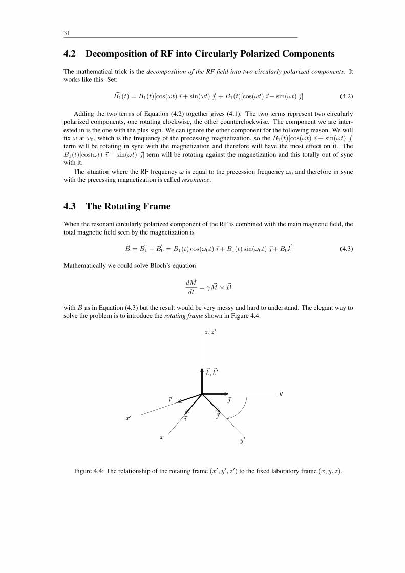
with ~B as in Equation (4.3) but the result would be very messy and hard to understand. The elegant way tosolve the problem is to introduce the rotating frame shown in Figure 4.4.
x′
xy′
y
z, z′
~ı′
~ı ~′
~
~k,~k′
Figure 4.4: The relationship of the rotating frame (x′, y′, z′) to the fixed laboratory frame (x, y, z).
A Course in MRI 32
Mathematically, the rotating frame’s x′–y′ unit vectors, ~ı′ and ~′, are related to the fixed frame’s x–yunit vectors,~ı and ~ by
~ı′(t) = ~ı cosω0t+ ~ sinω0t
~′(t) = −~ı sinω0t+ ~ cosω0t
(z and z′ are aligned). Visually, imagine a merry-go-round with the x–y axes painted on the ground under-neath it and the x′–y′ axes painted on the merry-go-round itself. Shrinking the merry-go-round to nuclearsize should give you an idea of what the rotating frame is all about.
The rotating coordinate frame rotates with the magnetization vector when it is precessing. From thepoint of view of the rotating frame the effective magnetic field looks very simple:
~Beff = B1(t)~ı′.
The effective field is along the x′ direction and all other components are zero. The effect of the mainfield,B0, is gone because, in the resonant rotating frame the magnetization has no angular momentum aboutthe z′ axis – it is cancelled out by centrifical force1. The form of the applied RF magnetic field therefore issimplified greatly in the rotating frame. This shows the point of applying a resonant frequency RF pulse.Physically, one of the circularly polarized components of the RF follows the magnetization around so that,as we’ll see next, the magnetic field B1 can affect ~M even though B1 is much, much smaller than B0.
Some readers may be uncomfortable with the disappearance of the B0 field in the rotating frame. Solet’s consider a frame that is rotating at a frequency not necessarily at the resonant frequency ω0. In thatcase
~Beff = B1(t)~ı′ + (B0 − ω/γ)~k′. (4.4)
The ω/γ term is the centrifugal force term. It cancels B0 when ω = ω0 = γB0. The centrifugal force termis there because the magnetization is intertwined with its angular momentum through γ. (See Exercise 1 atthe end of the chapter for the details.)
4.4 The Bloch Equations in the Rotating Frame
If we define the magnetization in the rotating frame by ~m = mx′~ı′ +my′
~′ +mz′~k′ then
Mx = mx′ cos(ω0t)−my′ sin(ω0t)
My = my′ sin(ω0t) +my′ cos(ω0t)
Mz = mz′
and the Bloch equation components in the rotating frame are:
dmx′
dt= 0
dmy′
dt= γB1(t) mz′ (4.5)
dmz′
dt= −γB1(t) my′
If B1(t) = B1, a constant, then the solution is:
mx′(t) = mx′(0)
my′(t) = my′(0) cos(ω1t)−mz′(0) sin(ω1t) (4.6)mz′(t) = my′(0) sin(ω1t) +mz′(0) cos(ω1t)
1The laws of physics, like Newton’s second law, are stated with respect to an inertial frame which is a reference frame that isneither accelerating nor rotating. The rotating frame is not an inertial frame and generates an artificial angular momemtum that mustbe subtracted to make the laws of physics correct. At the resonance frequency, this correction for the artificial angular momentumcancels the B0 term.

33
where ω1 = −γB1. Compare the solution (4.6) with the solution of the Bloch equation given by Equation(3.12). If you replace x′ by z and y′ and z′ by x and y respectively, you get the same solution, whichwe know to be a precessing solution. So in the rotating frame the magnetization precesses about the ~B1
magnetic field along the x′ axis as shown in Figure 4.5.
x′
y′
z′
~B1
~m
Figure 4.5: In the rotating frame, an RF field in the x′ direction causes the precession of ~m about the x′
axis.
4.5 90o and 180o RF Pulses
By turning the RF on and off, i.e. by having B1(t) = 0 before t = 0 and after t = T , we can control theangle through which ~M precesses. This is angle, α , is called the flip angle or tip angle and is given by
α = −γ∫ T
0
B1(t) dt. (4.7)
It happens that the only signal generated in an MRI comes from the x–y (or x′–y′) component of themagnetization.
When the patient or volunteer is first loaded into the MRI, all the magnetization is along the z direction.The application of a short RF pulse such that α = 90o will tip the magnetization vector completely into thex–y plane and a signal will be generated in the RF pick-up or receive coil.
In the case that B1 can be sharply turned on and off, its shape will look like that shown in Figure 4.6.So Equation(4.7) becomes α = −γbT for such a square pulse.
By either doubling the amplitude b or duration T one gets a 180o pulse that will tip the magnetizationfrom the +z direction to the −z direction.
Since there is no signal after a 180o pulse, the magnetization is said to be saturated. The magnetizationwill not stay oriented along the −z axis forever when relaxation is taken into account; the magnetizationwill recover to the +z axis and will be available for signal generation later.
To kill the magnetization for a longer time, imagers use what is called a saturation pulse. A saturationpulse precesses the magnetization vector around many, many times. Then, because of factors that wehaven’t incorporated into our simple model (the magnetization will be completely dephased), it will take awhile for the magnetization to recover to the +z direction again.
So, beware, there are two meanings for the word saturation in MRI.

A Course in MRI 34
B1
b
0 tT
Figure 4.6: The envelope B1(t) when it can be turned sharply on and off.
4.6 Chemical ShiftOur model for magnetization has, so far, considered that only one Larmor frequency was present. In realitythere will be many proton Larmor frequencies even if the main field B0 is perfectly uniform. This isbecause the protons will be the nuclei of hydrogen atoms that are part of different molecules. The mostabundant molecules in the human body are water and lipids. Different molecules have different electronicconfigurations that shield and modify B0 as seen by the hydrogen nucleus. Therefore the protons in thedifferent molecules will have slightly different Larmor frequencies. The resulting shift of frequencies iscalled chemical shift.
4.7 Inhomogeneities and Magnetic GradientsTwo other factors can contribute to a spread of Larmor frequencies. Both involve direct modification of B0.Those factors are:
1. Inhomogenities: variations in B0 over the volume of the body being imaged due to imperfections inthe field as actually built.
2. Gradients: these are linear variations in B0 introduced on purpose for imaging or slice selection.More will be said about gradients in Chapter 5.
4.8 Hard and Soft RF PulsesUsing a more complicated model that takes into account a magnetization population with varying Larmorfrequencies one can come the following conclusions:
1. Hard RF pulses, that is those of very short duration T and high amplitude b, tend to tip all of theLarmor frequencies equally. So a hard RF pulse can bring both water and lipid proton magnetizationto the x–y plane at the same time.
2. Soft RF pulses, that is those of longer duration T and smaller or softer amplitude b, tend to only tipmagnetization of a specific Larmor frequency.
With soft RF pulses, the shape of the function B1(t) becomes very important. So that if we have twofunctions with the same area under the curve, the tip angle will be different for different Larmor frequencymagnetizations. For example, the two functions for B1 shown in Figure 4.7 have (roughly) the same areaunder the curve (same integral) but the tip angles will be the same only for spins precessing at ω0.

35
����������������������������������������������������������������������������������������������������������������
����������������������������������������������������������������������������������������������������������������
����������
����������
B1
t
Figure 4.7: A hard RF pulse (left) and a soft RF pulse (right) having the same integral. The tip angles atω0 will be the same for both pulses, but at increasing off resonance frequencies the tip angles will fall offfaster for the soft RF pulse than for the hard RF pulse.
The pulses will only turn all the different Larmor frequency magnetization through the same angle only ifthey are “hard”. Some common RF shapes used in MRI are shown in Figure 4.8.
Sinc(∼ sin(Bt)
Bt
)
Gaussian(∼ Be−At2
)
Hyperbolic Secant
Figure 4.8: Some common RF (B1(t)) envelopes.
4.9 RF ReceptionWe mentioned that signal can only be generated by magnetization in the xy plane. This is because the signalis picked up only by a coil placed perpendicular to the xy plane as shown in Figure 4.9.
The magnetic field of the magnetization ~M then “cuts” the coil continuously, generating a voltageacross the open ends. The principle involved is exactly the same principle used by generators to generateelectricity for our homes. The principle is called Faraday’s Law and states that magnetic fields whose lines

A Course in MRI 36
z
x
y
coil in zy plane
~M
Figure 4.9: An RF coil is only sensitive to magnetization in the transverse, xy, plane.
of force move relative to a conduction medium (a wire) will generate a voltage in that conducting medium.In the case of an electrical generator, the wire moves while the magnetic field remains stationary. In MRI,the magnetic field of ~M moves while the voltage is generated in the stationary coil wires.
In practice, a loop such as that shown above won’t be very useful because it would block the patient’sentry into the MRI. A more typical configuration, say for a head coil, might use a saddle configuration thatlooks more like that shown in Figure 4.10.
x
y
z
two “saddle” coils
Figure 4.10: Saddle coil configuration. With saddle-type designs, the precessing magnitization will cut thewires that are parallel to the z axis.

37
Exercises1. *In an inertial frame, Newton’s law applied to rotation is
d ~J
dt= ~T
where ~J is angular momentum and ~T is torque (see Equation (3.11)). But a rotating frame is notinertial and we must add in the effects of centrifugal and Coriolis “forces”. We are not consideringany translational motion of the spins in a rotating frame so we only need to worry about (gyroscopic)centrifugal effects. In a frame with rotation given by ~ω (right rand rule), Newton’s law becomes
d ~J
dt= ~T − ( ~J × ~ω).
Using ~T = ~M × ~B and ~M = γ ~J , show that we may write the equation of motion for ~M as
1
γ
d ~M
dt= ~M × ~Beff
where~Beff = ~B − 1
γ~ω.
So that, in particular, if the z component of ~B is B0 and ~ω = ω~k then the z component of ~Beff isB0 − ω/γ as given in Equation (4.4). Hint: This exercise is very easy if you use the linear propertiesof the cross product: ~A× ~B + ~A× ~C = ~A× ( ~B + ~C) and ~A× (b ~B) = b( ~A× ~B).

A Course in MRI 38
Chapter 5
Slice Selection
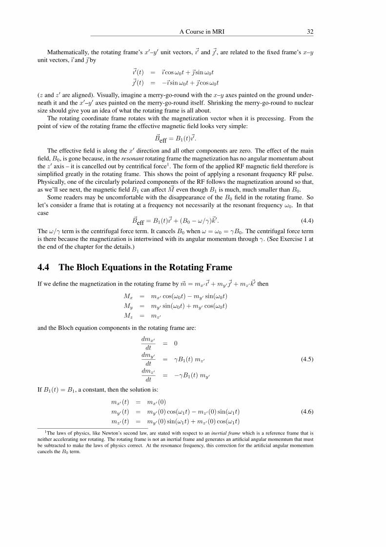
Slice selection is the excitation of magnetization only in a thin slice through a body as shown in Figure 5.1.
x
z
y
Only spins in thisslice will be tippedinto the xy planeafter the slice isselected.
Figure 5.1: The idea of an imaging slice.
The orientation of a slice may be arbitrarily chosen1. Anatomically, there are 3 principal, orthogonal sliceorientations in the body: axial (or transverse), saggital and coronal. Figure 5.2 illustrates MRI brain imagestaken in the three principal slice orientations.
axial sagittal coronal
Figure 5.2: MRI images in the three principal anatomical directions.
To understand slice selection and imaging, we now have to consider the magnetization as a functionin space (R3) instead of as a single vector at the origin of R3. We write ~M(~p) instead of just ~M . ~M(~p)
1The ability to choose slices in any direction makes MRI more flexible than an x-ray Computer Aided Tomography (CAT) scanwhich can only give axial slices.
39

A Course in MRI 40
represents a magnetization vector at the point ~p = (x, y, z) in space. For every ~p in space, there is amagnetization vector as shown in Figure 5.3.
x
z
y
~M(0, 0, 0)
~M(1, 1, 1)
Figure 5.3: A magnetization vector field.
So ~M is now a vector field instead of just a single vector. ~M is a collection, now, of the vectors ~M(~p) for all~p ∈ R3 (of course, the magnetization of points outside the body will be zero). Each ~M(~p) are individuallygoverned by the Bloch equation so, more completely, we need to consider magnetization as a function ofboth space and time: ~M(~p, t).
Fine point: Recall that the magnetization ~M is the expectation value 〈~µ〉 of magnetic moment andthat ~M represents the deterministic behavior of an ensemble of billions of nuclear spins. The atom is sosmall that our Bloch equation model considers that these billions of nuclei exist all at one point ~p in space.The reason for considering that the ensemble for 〈~µ〉 occupies a mathematical point is so calculus can theused to analyze the physics. The vector field model for ~M is called a continuum model and is actuallyan approximation made to make the math easier. The continuum magnetization model works because theactual resolution available in MRI is billions of times larger than the effective size of atoms.
5.1 Gradient Fields
The construction of an MRI includes 3 gradient field coil sets, one for each of the x, y and z directions.Their effect on the magnetic field is as follows.

41
1. x-direction — The x-gradient coil produces a linear variation of the magnetic field in the x-direction.When the x-gradient, Gx, is on the magnetic field is:
~B(x) = (Gx x+B0) ~k (5.1)
It makes the magnetic field a linear function of space in the x-direction. Graphically, Equation (5.1)defines a vector field that looks like that shown in Figure 5.4.
2. y-direction — The y-gradient, Gy , produces the field
~B(y) = (Gy y +B0) ~k (5.2)
which looks like that shown in Figure 5.5.
3. z-direction — The z-gradient, Gz , produces the field:
~B(z) = (Gz z +B0) ~k (5.3)
which looks like that shown in Figure 5.6.
4. all directions — The x,y and z gradients can all be turned on at once; then the magnetic field willbe:
~B(~p) = ( ~G · ~p+B0) ~k (5.4)
where the dot product (inner product) of ~G and ~p is indicated and
~G = (Gx, Gy, Gz)
is a vector that summarizes the gradient field contributions. Equation (5.4) describes a magnetic fieldin the z direction that varies linearly in the direction of ~G.
Physically, each of Gx, Gy and Gz are numbers that are directly proportional to the current flowingthrough the x, y and z gradient coils, respectively. Note that in all cases the magnetic field direction isalways in the z direction, but the magnitude varies as a function of spatial position.
When used in concert with a soft RF pulse, a slice perpendicular to ~G will be excited.
x
y
z
linearly varying with x
Figure 5.4: An x gradient field.

A Course in MRI 42
x
z
y
linearly varying with y
Figure 5.5: A y gradient field.
x
y
z
linearly varying in the z direction
B0
Figure 5.6: A z gradient field.

43
5.2 Slice Selection
Slice selection is accomplished by applying soft RF pulses, typically as a 90o pulse, while the gradients areon. With the soft RF pulse, the tip angle will be a strong function of the resonant frequency γB. The spinson the plane where ~B = B0
~k will tip as commanded. The spins away from that plane will not tip sincetheir resonant, Larmor, frequency will be different from the frequency of the RF pulse. The slice planewill be perpendicular to the vector ~G and the position of the slice plane can be moved by changing the RFfrequency as shown in Figure 5.7.
slice if RF ω < γB0 slice if RF ω = γB0 slice if RF ω > γB0
~G
Figure 5.7: Changing the RF frequency changes the position of the selected slice along the ~G direction.
5.3 Slice Profile
If we map the magnitude of the transverse (xy) component of the magnetization after a 90o “slice-select”RF pulse in the direction perpendicular to the slice plane, we get the slice profile shown in Figure 5.8.
Mxy
Here Mxy =√M2x +M2
y .
~G
Figure 5.8: A slice profile.

A Course in MRI 44
It turns out that there is a well-defined relationship between the slice profile and the RF pulse shape. Therelationship is called the Bloch transform and (to first order) can be approximated by the Fourier transform.So one can design a desired profile through the specfication of the RF pulse shape or, more precisely,through the specfication of the RF’s envelope shape.
Bloch Transform
MxyB1
~Gt
Figure 5.9: The slice profile is the Bloch transform of the RF envelope. To first order the Bloch transformis a Fourier transform.
When it comes to determining slice thickness, the mathematical properties of the Bloch transform2 arevery similar to the Fourier transform. So one can think about the properties of the Fourier transform tobuild up an intuition of the factors that influence slice thickness. The Fourier transform converts a functionwith a wide base or support to a function with a narrow support and vice versa. So, for example, an RFpulse envelope with small support (a hard RF pulse, with short temporal duration) leads to a slice profilewith a wide support – a thick slice. This is why a hard RF pulse will tip spins with a larger range ofLarmor frequecies than a soft RF pulse, which has large support (long duration). Mathematically speaking,functions of short duration have high frequency components. If you have something that happens quickly,you need short duration (high frequency) sinusoidal functions to describe it. We’ll have more to say aboutFourier transforms in Chapter 8.
Another way to make slices thinner is to increase the gradient field amplitude. The higher the gradient,the more rapidly the Larmor frequency changes as a function of distance. So there are two ways to make aslice thinner, use a higher gradient or use a softer RF pulse (or a combination of both). And there are twoways to make a slice thicker, use a lower gradient or use a harder RF pulse.
5.4 Partial Volume EffectWhen several slices are imaged sequentually, the overlapping slice profiles can cause the signal from oneslice to appear in the signal for another slice as shown in Figure 5.10.
The cross talk between slices is known as the partial volume effect because part of the volume from aneighboring slice can affect the signal in the slice of interest. The cross-talk can be minimized by acquiringthe slices in the order 1-3-5-2-4 in the above example instead of 1-2-3-4-5. This interleaving allows moretime for the magnetization in the neighboring signal to relax or decay so that it won’t have any signal leftfor cross-talk.
2The Bloch transform is derived from solutions to the vector field version of the Bloch equation as given by Equation (4.5) withgradient terms such as that given in Equation (5.4) added. The selection of an input B1(t) and ~G(t) (which, for simple cases isconstant) leads to an output mxy . The Bloch transform is approximated by the Fourier transform when the gradient field is heldconstant. References [7] and [8] have more information about the Bloch transform from a mathematical point of view.

45
overlapping slice profiles
~G
1 2 3 4 5
Figure 5.10: The slice profiles from nearby slices can overlap if the slice thickness is large relative to theslice spacing.

A Course in MRI 46
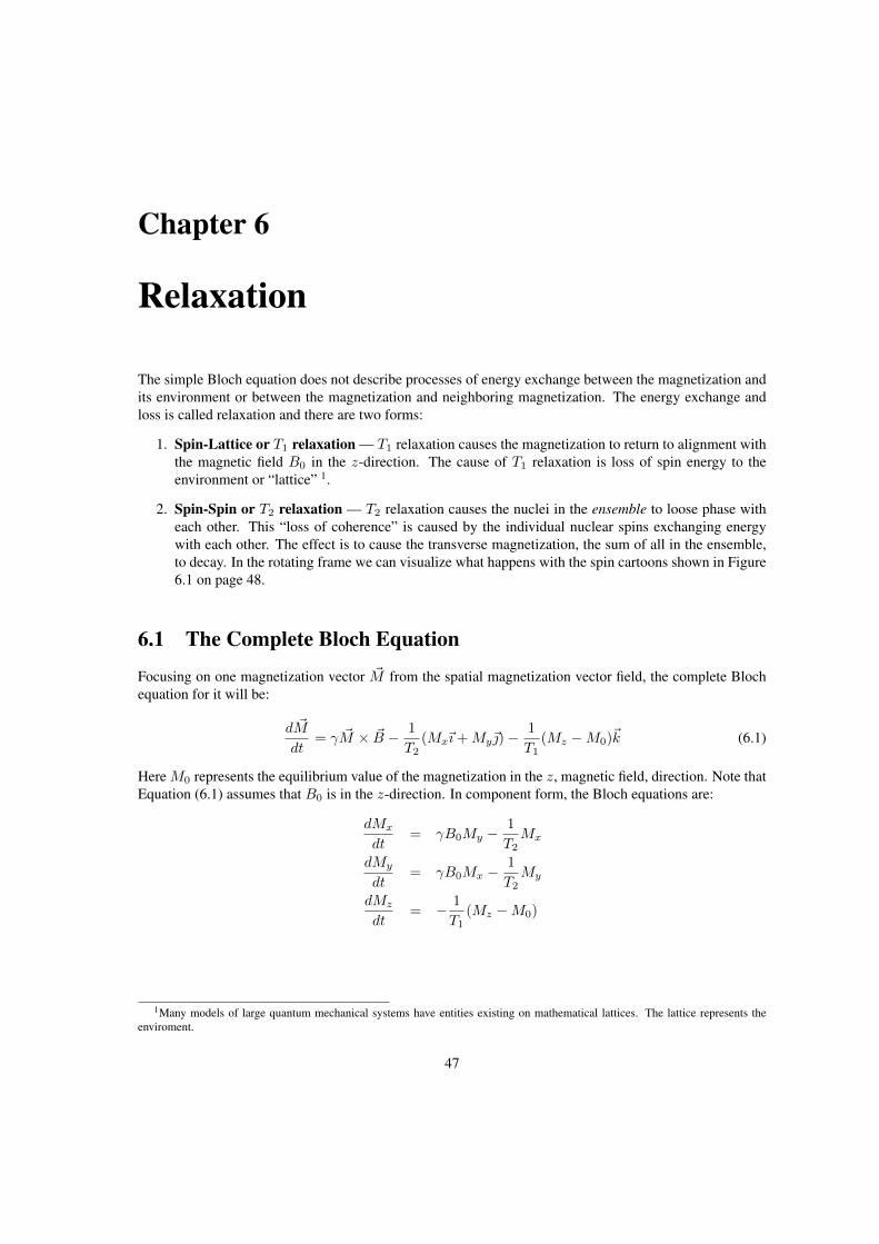
Chapter 6
Relaxation
The simple Bloch equation does not describe processes of energy exchange between the magnetization andits environment or between the magnetization and neighboring magnetization. The energy exchange andloss is called relaxation and there are two forms:
1. Spin-Lattice or T1 relaxation — T1 relaxation causes the magnetization to return to alignment withthe magnetic field B0 in the z-direction. The cause of T1 relaxation is loss of spin energy to theenvironment or “lattice” 1.
2. Spin-Spin or T2 relaxation — T2 relaxation causes the nuclei in the ensemble to loose phase witheach other. This “loss of coherence” is caused by the individual nuclear spins exchanging energywith each other. The effect is to cause the transverse magnetization, the sum of all in the ensemble,to decay. In the rotating frame we can visualize what happens with the spin cartoons shown in Figure6.1 on page 48.
6.1 The Complete Bloch Equation
Focusing on one magnetization vector ~M from the spatial magnetization vector field, the complete Blochequation for it will be:
d ~M
dt= γ ~M × ~B − 1
T2(Mx~ı+My~)−
1
T1(Mz −M0)~k (6.1)
Here M0 represents the equilibrium value of the magnetization in the z, magnetic field, direction. Note thatEquation (6.1) assumes that B0 is in the z-direction. In component form, the Bloch equations are:
dMx
dt= γB0My −
1
T2Mx
dMy
dt= γB0Mx −
1
T2My
dMz
dt= − 1
T1(Mz −M0)
1Many models of large quantum mechanical systems have entities existing on mathematical lattices. The lattice represents theenviroment.
47

A Course in MRI 48
1. Original state after 90o RF pulse. 2. After some time the individual ~µ makingup ~M dephase because energy givenfrom one nucleus to another causesone to speed up and the other to slow.The resultant vector sum of ~µ,~M , is therefore smaller.
x
z
y
x
z
y~M
~µ
~M
3. Eventually the nuclear spins will be completelyout of phase and there is no transverse ~M .
~µ
x
y
z
Figure 6.1: With (x, y, z) representing coordinates in the rotating frame we can visualize the T2, or spin-spin, relaxation process as irreversible energy exchange between the individual magnetizations ~µ that makeup the (“microscopic” – see section 6.2) ensemble ~M . ~M is the vector sum of all the individual ~µ whichrandomly exchange energy with each other. The exchange of energy between two spins will increase theLarmor frequency of one ~µ spin while equally decreasing the Larmor frequency of the other because energyis conserved.

49
Note the extra relaxation terms over the simple Bloch equation. It is a very involved matter to derivethe relaxation terms from quantum mechanical principles2. But these equations were not originally derivedfrom theory. Bloch originally proposed his equations as phenomnological; they are based on experimentalobservation.
The solutions of Bloch’s equations are given by:
Mx(t) = e−tT2 (Mx(0) cosω0t−My(0) sinω0t)
My(t) = e−tT2 (Mx(0) sinω0t+My(0) cosω0t)
Mz(t) = Mz(0)e−tT1 +M0(1− e−
tT1 )
The behavior of the transverse (xy) component is still to precess about the z-axis as with the simpleBloch equation, but now its magnitude decays according to e−
tT2 . So, suppose the initial transverse mag-
netization isMxy(0) =
√Mx2(0) +My2(0)
then the decay looks like the graph plotted in Figure 6.2.
Mxy
Mxy(0)
0.37Mxy(0)
T2
t
Figure 6.2: The magnitude of the transverse magnetization, Mxy , under T2 decay.
Notice that, after a time of T2 ms, the magnetization is reduced by 63% (since e−1 ∼= 0.37). T2 is knownmathematically as the characteristic time of the exponential decay. Without the T1 term, the z componentMz stays constant at Mz(0). With the T1 term the z-component recovers to M0. This T1 recovery lookslike the graph plotted in Figure 6.3 on page 50.
Again, T1 is the characteristic time of the exponential recovery and Mz has recovered by 63% after atime T1. Note that after a 90o RF pulse, Mz(0) = 0. After a 180o RF pulse, Mz(0) = −M0. A usefulconvention is to take time t = 0 as occurring immediately after an RF pulse when applying the Blochequations.
6.2 T ∗2 DecayThe difference in size between the world of the atom and the everyday world, even under the microscope(at a scale of micrometers), is very large. So, for the purposes of our model for magnetization at a point,~M(~p), we can consider it as being composed of many ensembles of nuclei; an ensemble of ensembles. The
2The concept of density matrices in quantum mechanics is useful for that derivation. Details may be found in Slichter’s book [21]which gives an excellent overview of the physics of NMR.

A Course in MRI 50
T1
Mz(0)
M0
Mz
t
Figure 6.3: The value of the z-component of the magnetization, Mz , under T1 recovery.
behavior of a “single ensemble” of transverse spins is given by T2 relaxation. The dephasing of spins at the“single ensemble” level is not reversible.
However, consider that the magnetization ~M is composed of several smaller ensembles of magnetization~m. The population of ~m magnetizations can be put out of phase with each other by variations in B0 sincethe ~m’s now cover more that an infinitesimal region of space. The sum of ~m’s, ~M , can then be modeled as
decaying roughly by e− tT∗2 (see Figure 6.4). But, the T ∗2 decay can be reversed as we’ll see in Chapter 7.
Thus, T ∗2 , is not technically relaxation since relaxation is irreversible.
~M
~m
~M
x
y
z
x
y
z
t = 0 t > 0
Figure 6.4: T ∗2 decay is visualized in the rotating frame exactly as T2 decay but with ~M being the vectorsum from a mesoscopic ensemble that is large enough for inhomogenieties in the main magnetic field B0 tocause a Larmor frequency variation across the ensemble. The dephasing caused by those inhomogeneitiesare reversible by flipping the spins through 180◦. This is what the spin-echo sequence, discussed in Chapter7 does.
It is helpful to think of three levels of scale:
1. “microscopic” — The level of the individual ensemble. It is so small that there can be no variationof magnetic field within the ensemble. The spins in the ensemble exchange energy with each otherrandomly in quantum mechanical processes. The energy exchange causes a dephasing which could

51
only be reversed by exactly undoing the random energy exchange. Since the reversal of a randomsequence of events by chance is impossible, the dephasing at the single ensemble, or microscopic,level is irreversible. T2 relaxation happens at the microscopic level.
2. “mesoscopic” – The level of an ensemble of ensembles. Still unimaginably small but now variationsin the magnetic field are important. Magnetic field variations will cause the ensembles to get out ofphase with each other, but reversing the magnetic field varations will cause the spins to rephase. Thedecay caused by dephasing at the mesoscopic, ensemble of ensembles, level is therefore reversible.T ∗2 decay happens at the mesoscopic level.
3. “macroscopic” — The scale at the size of image pixels, roughly a square millimeter. You need allthe spins at this level (roughly around Avagadro’s number, 623) to produce a measureable signal.

A Course in MRI 52

Chapter 7
Pulse Sequences I
The process of producing an MR image requires the application of RF and gradient pulses in the correctorder. There are many combinations of pulses that can produce an image of a desired contrast. Such pulsesequences are best described graphically through timing diagrams structured as shown in Figure 7.1.
ADC
RxRF
TxRF
Gz
Gy
Gx
Preparation Measurement
Figure 7.1: A skeleton timing diagram. Here Gx = x-gradient, Gy = y-gradient, Gz = z-gradient, TxRF =RF Transmit, RxRF = RF Receive, ADC = Analog to Digital Conversion. The horizontal axis representstime. TxRF is essentially the B1 function of Equation (4.1) and its amplitude is a complex valued functionbecause the phase of the RF determines the tip precession axis in the rotating frame. The ADC is either on oroff. When it is on, the received RF (RxRF ) is digitized and stored on computer disk. By convention, we’llsay that an MRI signal exists when the ADC is on. Another convention would be to consider the voltagein the RxRF coil to be the signal. A pulse sequence program is a computer program written to producefunctions for each line in the timing diagram. These functions are provided as input to the appropriateamplifier via a digital signal processor (the computer program physically controls digital signal processorsor DSPs). The output of an amplifier is an amplified (much amplified in the case of the gradient amplifiers)version of the input.
As shown in Figure 7.1, pulse sequences can, generally, be divided into a preparation and measurementphase. Most imaging sequences intermix the preparation and measurement phases but they can still beseparated conceptually.
53
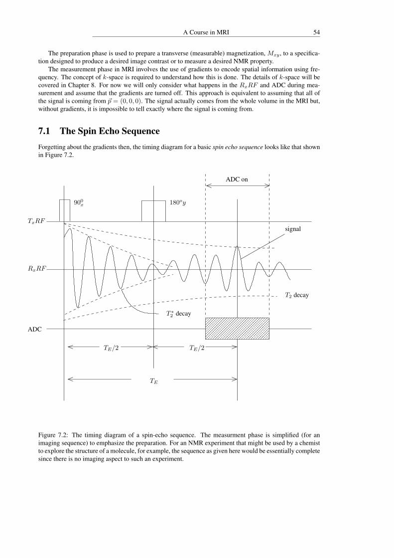
A Course in MRI 54
The preparation phase is used to prepare a transverse (measurable) magnetization, Mxy , to a specifica-tion designed to produce a desired image contrast or to measure a desired NMR property.
The measurement phase in MRI involves the use of gradients to encode spatial information using fre-quency. The concept of k-space is required to understand how this is done. The details of k-space will becovered in Chapter 8. For now we will only consider what happens in the RxRF and ADC during mea-surement and assume that the gradients are turned off. This approach is equivalent to assuming that all ofthe signal is coming from ~p = (0, 0, 0). The signal actually comes from the whole volume in the MRI but,without gradients, it is impossible to tell exactly where the signal is coming from.
7.1 The Spin Echo SequenceForgetting about the gradients then, the timing diagram for a basic spin echo sequence looks like that shownin Figure 7.2.
���������������
���������������
������������������������������
������������������������������
���������������������
���������������������
ADC
RxRF
TxRF
900x 180oy
signal
T2 decay
T ∗2 decay
ADC on
TE/2 TE/2
TE
Figure 7.2: The timing diagram of a spin-echo sequence. The measurment phase is simplified (for animaging sequence) to emphasize the preparation. For an NMR experiment that might be used by a chemistto explore the structure of a molecule, for example, the sequence as given here would be essentially completesince there is no imaging aspect to such an experiment.

55
~M
(1) t < 0,before 90ox RF pulse.
x
y
z
~M
(2) t = 0,just after 90ox RF pulse.
“individual ensemble”magnetizations, ~m
x
y
z
slower ~m
~M
faster ~m
(3) t slightly less than TE/2,just before 180oy RF pulse.
x
y
z
180o flip about y-axisfaster ~m
~M
slower ~m
(4) t just after TE/2,just after the 180oy RF pulse.
x
y
z
x
y
z
~m ~M
(5) t = TE .
In frame (5), magnetization that has dephaseddue to T ∗2 has rephased. Note that
~M(TE) = e−TE/T2 ~M(0); only the irreversibledecay due to T2 relaxation remains in ~M .
Figure 7.3: The main events in a spin echo sequence in terms of “spin cartoons”. The essential idea is tothink of a spin ensemble ~M as being composed of many sub ensembles ~m.

A Course in MRI 56
90x 180y 90x 180y 90x 180y 90x 180y
TE TE TE TE
TxRF
RxRF
ADC
TR TR TR
Figure 7.4: The “repetition time” between repeats of a spin echo sequence is TR. The spin echo sequenceneeds to be repeated to acquire spatial frequency information along different lines in k-space as explainedin Chapter 8.
The sequence contains a 90o RF pulse, a wait of time TE/2, a 180o pulse, and finally the signal is measured,centered at a time TE/2 after the 180o pulse. The time TE is known as the echo time because the RxRF“echoes” or reaches a local maximum TE ms after the 90o pulse. Notice that the RF pulses are written 90oxand 180oy; that means that the 90o tip angle is about the x-axis in the rotating frame and the 180o tip angleis about the y-axis in the rotating frame. (Note: the prime rotation, x′ and y′, used in Chapter 4 has beendropped. Similarly, we will use M instead of m to denote magnetization in the rotating frame.)
In the rotating frame, Fig. 7.3 shows what happens during a spin echo sequence.
7.2 Repeating Basic SequencesImaging sequences can require that a signal be acquired over and over again. In the case of a spin echosequence, for example, the repeated pulse sequence looks like that shown in Fig. 7.4.
The time between signal measurements, TR, is known as the repeat time. The length of TR affects theamount of Mz magnetization available for the 90o RF tip. Just after the 90o RF pulse, at t = 0, Mz(0) = 0.After a time TR, the z-magnetization will have recovered to
Mz(TR) = (1− e−TR/T1)M0. (7.1)
So, except for the very first 90ox degree RF pulse, the transverse magnetization immediately after a 90ox RFpulse is
My(0) = Mz(TR) = (1− e−TR/T1)M0 (7.2)
and, when the signal is measured,
My(TE) = e−TE/T2Mz(TR) = e−TE/T2(1− e−TR/T1)M0. (7.3)

57
The signal, which is proportional to the transverse magnetization at the measurement time, is a function ofT2 via TE , T1 via TR and the proton density, via M0. In Equations (7.1) – (7.3) the convention of resettingthe clock to t = 0 after every 90o RF pulse is used.
7.3 Weighting and Image ContrastA close inspection of Equation 7.3 shows that the effects of T1 relaxation or T2 relaxation, or both, may beremoved by appropriately selecting TR and TE . Explicitly:
• if TE is short then e−TE/T2 ∼= e0 = 1
• if TR is long then (1− e−TR/T1) ∼= 1− e−∞ = 1− 0 = 1.
So if TE is short, the effect of T2 on the signal will be small. If TR is long, the effect of T1 on the signalwill be small. And, of course, the converse is true. If TE is long, the effect of T2 on the signal will be largeand if TR is short, the effect of T1 on the signal will be large. With the values of T1 and T2 found in humantissue, a TR of more than 2000 ms or so is considered long, while a TE of less than 15 ms is consideredshort.
Different tissues have different values of T1, T2 and M0 because of differences in the tissue densityand in the tissue’s chemical and physical environment. As a general rule, tissues that are more watery havelonger relaxation times (both T1 and T2). In the brain, for example, white matter has a short T1 and T2 incomparison to grey matter. In comparison to both the white and grey matter, cerebral spinal fluid (CSF),being very “watery” or fluid, has very long relaxation times. A fluid enviroment allows less time for eachspin to exchange energy with something else – the spin is more separated from its environment and otherspins than in would be if it were held in place by a more solid environment. The differences in relaxationrates and proton density between tissues provides the basis for contrast in MRI. With the two variablesof TR and TE to play with in the pulse sequence, we can make images whose contrast is predominatelydetermined by T1, T2 or M0. Such images are called T1 weighted, T2 weighted or proton density weightedimages respectively and each will show different tissue contrasts.
To obtain T1, T2 or proton density weighted images, we simply choose the TR and TE in the pulsesequence so that one desired effect is larger than the other two. The approach can be summarized as shownin Table 7.1.
Short TR Long TR
Short TE T1 weighted proton density weighted
Long TE useless contrast mixture T2 weighted
Table 7.1: The effects of different combinations of TE and TR.
The appearance of the human brain with various contrast weighting can be seen in the images in Fig. 7.5,all of the same brain slice.

A Course in MRI 58
T1 weighted image
TR = 525 ms, TE = 15 ms
T2 weighted image
TR = 2500 ms, TE = 95 ms
Proton density weighted image
TR = 2000 ms, TE = 15 ms
Figure 7.5: Changing TR and TE to achieve T1, T2 and proton density weighted images leads to differentcontrasts between brain tissue types.

59
In the T1 weighted image, the short T1 of the white matter gives the highest signal because the zcomponent of the magnetization has almost completely recovered before each successive 90o RF pulse.The grey matter, having a longer T1 gives less signal and therefore appears darker. The CSF has the longestT1, being fluid, and so appears darkest. Grey matter is grey, white matter is white and CSF is black.
In the T2 weighted image, the short T2 of the white matter gives the lowest signal because the transverse(x–y) component of the magnetization has almost completely decayed by the time the signal is measured.The grey matter, having a longer T2 gives more signal and therefore appears brighter. The CSF has thelongest T2, being fluid, and so appears brightest. Grey matter is grey, white matter is black and CSF iswhite.
The proton density weighted image directly shows the density of water molecules in the brain, wherethe hydrogen nuclei are located. Grey matter is denser than white matter which is denser than CSF. Greymatter is white, white matter is grey and CSF is black. Actually, a closer comparison of the proton densityimage with the T1 image shows that not all of the white matter shows up as grey in the proton density image.Only a particular aspect of the white matter gives contrast in the proton density image. With the TR of 2000ms used the make the image above, there is still some T1 contrast in the CSF. At a longer TR, say 3000 ms,there will be no contrast between the CSF and grey matter.
As a rough rule of thumb, radiologists typically use T1 weighted images to see structural anatomicaldetail and T2 weighted images to look for abnormal tissue contrast (e.g. tumors).
7.4 Slice Selection in a Pulse SequenceRecall that slice selection is the result of applying soft RF pulses in the presence of gradients. In the caseof the spin echo sequence, one or the other or both of the 90o or 180o pulses may be slice-selective. Whenacquiring multiple slices, both pulses should be slice selective. For a slice perpendicular to the x-axis,the slice selective timing diagram for a spin echo sequence, with two slice selective pulses, looks like thatshown in Fig. 7.6.
Gx
TxRF
RxRF
ADC
90x 180y
t = 0 t = TE/2 t = TE
Figure 7.6: Slice selection is achieved with a combination of soft RF pulses in the presence of magneticfield gradients.
Note that there is a negative Gx pulse immediately following the 90o RF/gradient application. Thepurpose of the negative Gx pulse is to “refocus” magnetization at the top and bottom of the slice profile.The magnetization at the top of the profile will have a Larmor frequency higher than the middle of the sliceand the magnetization at the bottom of the slice profile will have a Larmor frequency lower than the middle

A Course in MRI 60
of the slice. So, during the time it takes for the magnetization to tip through 90o, the magnetization at thetop will be ahead, and the magnetization at the bottom of the slice profile will be behind, the magnetizationat the middle of the profile, see Fig. 7.7.
~M from bottomof slice profile
~M from middleof rf slice profile
~M from top ofslice profile
After 90oRF pulse, before negative Gx pulse.
~M
After negative Gx.
x
y
z
x
y
z
Figure 7.7: Spins perpendicular to the intended slice precess at different Larmor frequencies, so they needto be refocused after a 90◦ RF pulse.
The negative Gx pulse makes the Larmor frequencies at the top of the slice profile slow and the ones at thebottom fast to allow all the spins in the profile to re-align with each other.
7.5 Acquiring Signal from Multiple SlicesIn order to have enough Mz to generate a signal, the TR must be a large fraction of T1. This may mean, forexample, that TR has to be as a long as 2 or 3 seconds (2000 to 3000 ms) when a proton density image isdesired. A single spin echo acquisition only requires a time of TE which is, perhaps, only 15 ms. There is alot of dead time between acquisitions caused by a long TR. The dead time can be used to acquire signal fromother slices. For example, suppose we want to image 4 slices in the x-direction. Then the timing diagramwould look like that shown in Fig. 7.8. The different slices are defined by using different RF frequencies,as we saw before. Note that with a longer the TR, more slices can be obtained. The maximum number ofslices, Nmax, that can be acquired for a given sequence is
Nmax < TR/TE . (7.4)
Since the 90o RF pulse and the ADC events do not occur instantaneously, it will require a few moremilliseconds over TE to acquire the signal from one slice. So we can’t quite have equality in Equation (7.4).Recall, also, that we need to worry about partial volume effect when setting up a multiple slice sequence.The slices 1, 2, 3 and 4 in the sequence could be acquired sequentially as a stack. That is, they could bearranged as shown in Fig. 7.9, top left. But, as we saw in Chapter 5, if the slices are close together, theirprofiles could overlap as shown in Fig. 7.9, bottom. The signal from a slice will die off due to T2 relaxationif you wait long enough. So, to minimize the cross-talk, the signal in the neighboring slice should be giventime to die out. As we saw before, instead of stacking slices, a better scheme is to interleaf them as shownin Fig. 7.9, top right. Switching from stacked to interleaved slices is accomplished by changing the order ofRF frequencies used during slice selection. In this example, the interference in slice 1 from the neighboringslice is reduced because the magnetization in the neighboring slice has had twice the time to decay thanit would have with the stack scheme. With a small number of slices, it may be impossible to completely

61
slice 1 2 3 4 1 2 3 4 1 2 3 4
Gx
TxRF
RxRF
ADC
TR TR
TR TR
TR TR
TR TR
Figure 7.8: Multiple slices can be acquired during the TR interval.
avoid the partial volume effect. For example, there is still some interference between slices 2 and 3 inthe interleaved scheme illustrated above. In such cases, one could try to add another slice or increase thespacing between the slices so that slice cross-talk is no longer a problem.

A Course in MRI 62
x
y
z
slice 1
slice 2slice 3
slice 4
slice 1
slice 3slice 2
slice 4
x
y
z
slice 4 slice 3 slice 2 slice 1
y
x
Figure 7.9: Top Left: Acquiring the slices in simple sequence can lead to cross-talk because the transversemagnetization from the last slice hasn’t completely decayed and contributes to the signal of the new slice.Top Right: Interleaving the slice acquisition gives time for the transverse magnetization from the last sliceto decay. Bottom: Signal in the slice profile overlaps causes slice cross-talk if the transverse magneti-zation from the previous acquisitions hash’t had a chance to decay. Interleaving gives more time for themagnetization in a slice to decay before the spatially neighbouring slice is acquired.
7.6 Multiple Echo T2 or Multiple Spin EchoBy adding a series of 180o RF pulses to the basic spin echo sequence, the transverse magnetization can bemade to refocus over and over again. With each refocusing, however, the signal will be lower and lowerbecause of T2 relaxation. The multiple echo T2 sequence, for an example with four spin echoes, looks likethat shown in Fig. 7.10.
• It is not necessary for TE1 = TEA = TEB = TEC . The effective echo times for each RF echo can bechosen arbitrarily.
• Each echo can be used to make an MR image.
• With the multi-echo sequence, T2 can be measured by finding the best, least squares, exponentialcurve fit through the signal points at the echo times.

63
90ox 180oy 180oy 180oy 180oy
TxRF
RxRF
ADCTE1 TEA TEB TEC
TE2
TE3
TE4
envelope ofT2 decay
Figure 7.10: A multiple spin echo sequence with 4 echoes.
Exercises1. Suppose you are acquiring some T1 weighted MRI images with TR = 525 ms and TE = 15 ms.
What is the maximum number of slices that can be obtained with the sequence?
2. Why is a negative gradient application not required after the 180o RF pulse?

A Course in MRI 64

Chapter 8
K-Space
The concept of k-space is required to understand how an image can be made from an NMR signal. k-spaceis a mathematical concept related to Fourier transforms, so a brief review of Fourier transforms is requiredbefore we can understand k-space. Fourier transforms, in turn, transform one complex-valued function intoanother. So we begin with a review of complex numbers and complex-valued functions.
8.1 Complex Numbers: Magnitude and PhaseRecall that a complex number, a, is a two-dimensional number with a real and imaginary part, a = aR+iaI ,and can be represented as a point on the Argand plane as shown in Fig. 8.1.
Imaginary
Real
aI
α
|a|
aR
Figure 8.1: A complex number a, shown here as a big dot plotted on the Argand plane, has a real compo-nent, aR, and an imaginary component, aI . On the Argand plane, the usual x direction is the real direction,and represents the number line where all real numbers live. The usual y direction is the imaginary direc-tion where i =
√−1 lives where y = 1 usually lives. A complex number may also be represented by
its magnitude |a| and its phase α instead of its real and imaginary parts. A complex number is a two-dimensional number that requires two real numbers, real and imaginary parts or magnitude and phase parts,to completely represent it.
A complex number can also be represented by magnitude and phase, a = |a| eiα, as shown in the diagram
65

A Course in MRI 66
of Fig. 8.1. The phase, α, is also known as the argument of a. |a| is the magnitude of a. The relationshipbetween the two representations of a complex number is given by
|a| =√a2R + a2
I α = tan−1(aIaR
)aR = |a| cosα aI = |a| sinα
The notation eiα can be therefore written
eiα = cosα+ i sinα
soa = |a| eiα = |a| cosα+ i |a| sinα.
The magnitude and phase representation is useful for multiplying and dividing complex numbers:
ab = |a|eiα · |b|eiβ = |a| · |b|ei(α+β)
a/b = (|a|eiα)/(|b|eiβ) = (|a|/|b|)ei(α−β).
The real and imaginary notation is useful for adding and subtracting complex numbers.
8.2 Complex Valued FunctionsBefore we introduce complex valued functions, a quick review of real-valued functions may be useful.
8.2.1 1D real-valued functions1D real-valued functions may be characterized from abstract to concrete as follows:
• A 1D real-valued function, f , is a map from the set of real numbers, R, to the set of real numbers, R,written symbolically as
f : R→ R.
• The function f maps the real number x to the real number y, with the value y being given symbolicallyby
y = f(x), x ∈ R, y ∈ R.
• A 1D real-valued function can be represented graphically, for example, as the familiar graph shownin Fig. 8.2.
y
f
x
Figure 8.2: A real-valued function, f , can be represented as a graph with the y co-ordinate of the line abovea point on the x-axis representing the value of the function f(x).

67
8.2.2 2D real-valued functionsSimilar to 1D real-valued functions, 2D real-valued functions may be characterized from abstract to con-crete as follows:
• A 2D real-valued function, f , is a map from the plane, R2, to the set of real numbers, R, writtensymbolically as
f : R2 → R.
• The function f maps the point ~p = (x, y) to z, with the value z being given symbolically by
z = f(x, y) = f(~p), where ~p = (x, y) ∈ R2, z ∈ R.
That is, f maps the point in the plane ~p to the real number z.
• A 2D real-valued function can also be represented graphically, for example as shown in Fig. 8.3.
x
y
z
Figure 8.3: A 2D real-valued function, f , can be represented as a surface in 3D space. The independentvariable in the domain is a point (x, y) in a plane, the value f(x, y) of the function is the z height of thesurface above (x, y).
3D real-valued functions are similar except that ~p ∈ R3 is a point in 3D space instead of a point on the 2Dplane R2. Since four dimensions are involved for a 3D real-valued function, a graph is difficult to draw.But it can be done by using color to represent the real value of the function. Now we can consider complexvalued functions.
8.2.3 1D complex-valued functions1D complex-valued functions may be characterized from abstract to concrete as follows:
• A 1D complex-valued function, f , is a map from the set of real numbers, R, to the set of complexnumbers, C, written symbolically as
f : R→ C.
• The function f maps the point x to y, with the value y being given symbolically by
y = f(x), x ∈ R, y ∈ C.
Note now that y = yR + iyI = |y| eiαy is a complex number. So f maps the real number x to thecomplex number y.

A Course in MRI 68
• It is difficult to draw a graph. One approach would be to draw a curve on the Argand plane thatrepresented the real number line (the domain1).
8.2.4 2D complex valued functions2D complex-valued functions may be characterized from abstract to concrete as follows:
• A 2D complex-valued function, f , is a map from the plane, R2 to the set of complex numbers, C,written symbolically as
f : R2 → C.
• The function f maps the point ~p = (x, y) to z, with the value z being given symbolically by
z = f(x, y) = f(~p), where ~p = (x, y) ∈ R2, z ∈ C
The number z is a complex number: z = zR + izI = |z| eiαz . So f maps the point in the plane ~p tothe complex number z.
• Since four dimensions altogether are involved two each in the domain and range it is impossible todraw a graph directly, although a vector field kind of drawing shows what is going on.
3D complex-valued functions are similar except that ~p ∈ R3 is a point in 3D space instead of a point on the2D plane R2.
8.3 Transverse Spin as a Complex NumberIn the rotating frame, a generic transverse magnetization will have both x and y components. The com-ponents can be expressed as the real and imaginary parts of a complex number. Let Mt be the transversemagnetization. Then
Mt = Mx + iMy = |Mt| eiθ = Mxyeiθ
where θ = tan−1(My
Mx
)and |Mz| = Mxy =
√M2x +M2
y .
8.4 There is a Transverse Magnetization Complex Number at EveryPoint in Space in MRI
The measured signal in MRI is solely due to the Mt complex numbers (vectors) at every point in space. SoMt is a complex-valued function on R3 (a 3D complex-valued function):
Mt : R3 → C.
Mt(~p) is the value of the transverse magnetization, as a complex number, at the point ~p = (x, y, z) in abody.
If only a slice has been excited then we may consider ~p ∈ R2 so that Mt : R2 → C. In this case, beaware that the R2 coordinates x and y are on the slice and that they do not have to match the global x, y, zcoordinates in which z is the main field direction.
1Recall that a function maps objects from a domain into a range.

69
As an example where the local slice coordinates are different from the global coordinates, we couldhave the situation shown in Fig. 8.4.
������������������
������������������
��������������������������������������������
x
z
local to slicey
x
y
Figure 8.4: If an obliquely oriented slice has been excited, it is convenient to define x and y coordinates onthe slice, when talking about slice sequences and Fourier transforms, instead of using the global co-ordinatesdefined by the z-axis of the B0 magnetic field.
Note that, as a complex valued function or as a vector field, the transverse magnetization (and the threecomponent ~M itself) is frequently referred to as a magnetization density. With that point of view, you haveto integrate over a small volume to get an actual magnetization. It is helpful to think in terms of densitywhen adding up the effect of all Mt(~p), by integration, to compute the MRI signal2.
8.5 1D Integral Fourier TransformA Fourier transform, F , is a function of functions. It maps one complex valued function f to anotherfunction f . Symbolically, F : f → f .
Let’s consider that f , a 1D complex-valued function, is a function of time, t. Then the Fourier transformof f , f , will be a function of frequency, η. The 1D integral Fourier transform of f is defined by:
f(η) =
∫ ∞−∞
f(t) e−2πiηt dt (8.1)
or, breaking it into real and imaginary parts (assuming f is real-valued; fI = 0):
f(η) =
∫ ∞−∞
f(t) cos(2πηt) dt− i∫ ∞−∞
f(t) sin(2πηt) dt. (8.2)
Instead of time t and frequency η, we can also have Fourier transforms of functions of distance or space,x. The corresponding spatial frequency is denoted with k. In that case, the integral Fourier transform iswritten:
f(k) =
∫ ∞−∞
f(x) e−2πixk dx.
What does the Fourier transform mean? It means that all functions (with some technical, mathematicalrestrictions) are composed of a weighted sum (the integration) of combinations of sines and cosines of every
2The density concept is an abstraction invented for mathematical convenience. In the abstraction, an individual spin is ~M(~p) d~pand is imagined as being infinitely small so that it only occupies a mathematical point. The magnetization associated with an ensemblewould then be
∫∫∫∆~M(~p) d~p where ∆ is the spatial volume occupied by the ensemble.

A Course in MRI 70
possible frequency. The weighting is given by the function itself! The Fourier transform is the mathematicalexpression of the Tao or Hindu idea that everything is composed of cycles.
A function f and its integral Fourier transform f together are known as a Fourier transform pair. Thebest known example of a Fourier transform pair is between the sinc function (the sinx/x function) and the“boxcar” function (which is equal to one on a finite interval and zero everywhere else), see Fig. 8.5.
f(x) = 2A sin(2πAx)2πAx
x
f(x)
F
F−1
f(k) =
{1 if −A ≤ x ≤ A0 otherwise
f(k)
−A A
k
f(x) =
{1 if −A ≤ x ≤ A0 otherwise
−A A
f(x)
F
F−1
f(k)
f(k) = 2A sin(2πAk)2πAk
Figure 8.5: The sinc function (sinx/x) and the boxcar function are a Fourier transform pair.
As hinted in Fig. 8.5, the Fourier transform is invertable. That is, if Ff = f , then F−1f = f whereF−1 denotes the inverse Fourier transform. We write F−1f = f . The inverse integral Fourier transform is
f(x) =
∫ ∞−∞
f(k) e2πikx dk. (8.3)
The difference in the formula for the Fourier transform and the formula for its inverse is the minus sign inthe exponent.
8.6 2D and 3D Fourier TransformsIf the spatial coordinate ~p is in R2 (so that ~p = (x, y)) or in R3 (so that ~p = (x, y, z)) then the spatialfrequency ~k will be in R2 (so that ~k = (kx, ky)) or R3 (so that ~k = (kx, ky, kz)) respectively.
In the R2 case, the integral Fourier transform is given by
f(~k) =
∫ ∞−∞
∫ ∞−∞
f(~p) e−2πi~k·~pd~p (8.4)
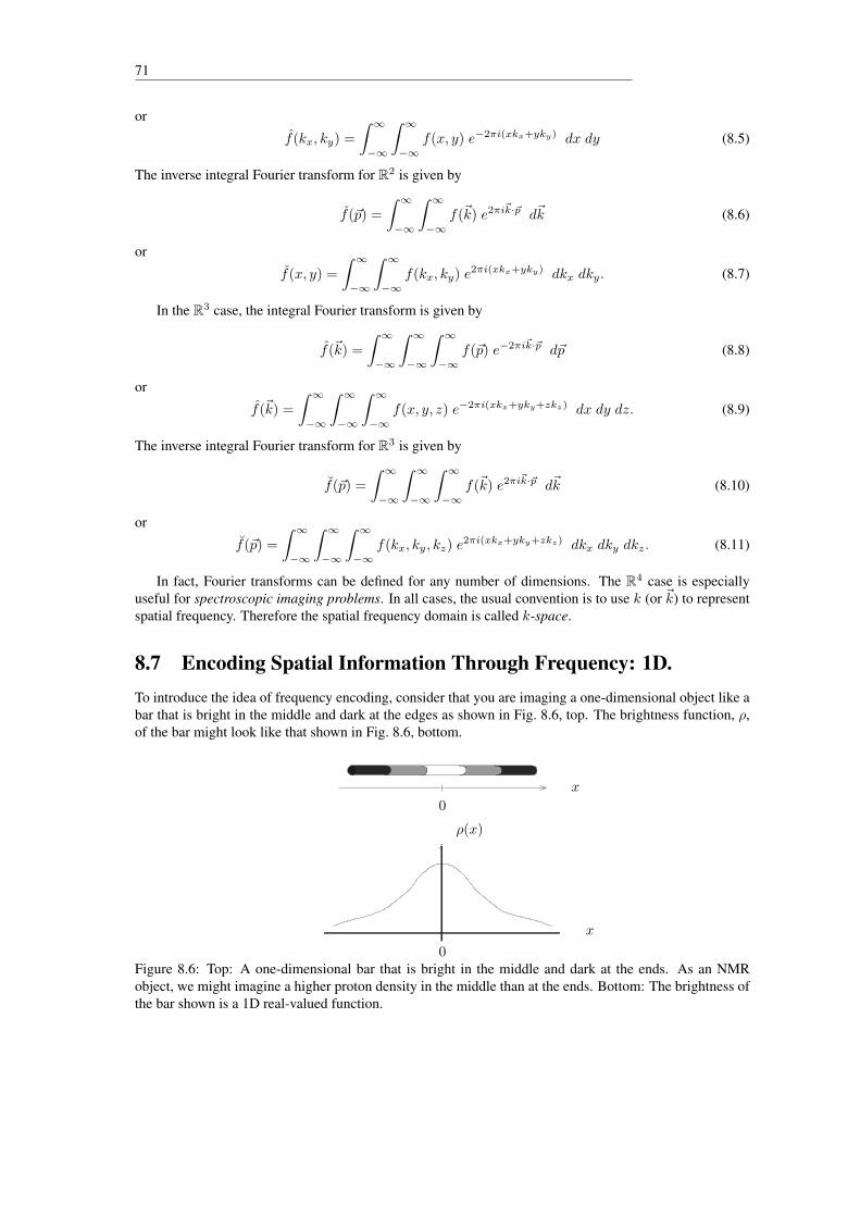
71
or
f(kx, ky) =
∫ ∞−∞
∫ ∞−∞
f(x, y) e−2πi(xkx+yky) dx dy (8.5)
The inverse integral Fourier transform for R2 is given by
f(~p) =
∫ ∞−∞
∫ ∞−∞
f(~k) e2πi~k·~p d~k (8.6)
or
f(x, y) =
∫ ∞−∞
∫ ∞−∞
f(kx, ky) e2πi(xkx+yky) dkx dky. (8.7)
In the R3 case, the integral Fourier transform is given by
f(~k) =
∫ ∞−∞
∫ ∞−∞
∫ ∞−∞
f(~p) e−2πi~k·~p d~p (8.8)
or
f(~k) =
∫ ∞−∞
∫ ∞−∞
∫ ∞−∞
f(x, y, z) e−2πi(xkx+yky+zkz) dx dy dz. (8.9)
The inverse integral Fourier transform for R3 is given by
f(~p) =
∫ ∞−∞
∫ ∞−∞
∫ ∞−∞
f(~k) e2πi~k·~p d~k (8.10)
or
f(~p) =
∫ ∞−∞
∫ ∞−∞
∫ ∞−∞
f(kx, ky, kz) e2πi(xkx+yky+zkz) dkx dky dkz. (8.11)
In fact, Fourier transforms can be defined for any number of dimensions. The R4 case is especiallyuseful for spectroscopic imaging problems. In all cases, the usual convention is to use k (or ~k) to representspatial frequency. Therefore the spatial frequency domain is called k-space.
8.7 Encoding Spatial Information Through Frequency: 1D.To introduce the idea of frequency encoding, consider that you are imaging a one-dimensional object like abar that is bright in the middle and dark at the edges as shown in Fig. 8.6, top. The brightness function, ρ,of the bar might look like that shown in Fig. 8.6, bottom.
0
x
0
ρ(x)
x
Figure 8.6: Top: A one-dimensional bar that is bright in the middle and dark at the ends. As an NMRobject, we might imagine a higher proton density in the middle than at the ends. Bottom: The brightness ofthe bar shown is a 1D real-valued function.
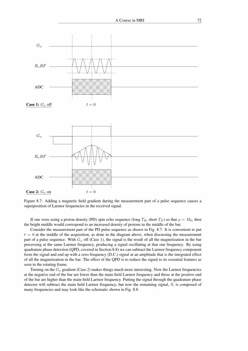
A Course in MRI 72
��������������
��������������
��������������������������������������������������
��������������������������������������������������
����������������������������������������
����������������������������������������
��������������������
����
����
Case 2: Gx on t = 0
ADC
RxRF
Gx
Case 1: Gx off t = 0
ADC
RxRF
Gx
Figure 8.7: Adding a magnetic field gradient during the measurement part of a pulse sequence causes asuperposition of Larmor frequencies in the received signal.
If one were using a proton density (PD) spin echo sequence (long TR, short TE) so that ρ = M0, thenthe bright middle would correspond to an increased density of protons in the middle of the bar.
Consider the measurement part of the PD pulse sequence as shown in Fig. 8.7. It is convenient to putt = 0 at the middle of the acquisition, as done in the diagram above, when discussing the measurementpart of a pulse sequence. With Gx off (Case 1), the signal is the result of all the magnetization in the barprecessing at the same Larmor frequency, producing a signal oscillating at that one frequency. By usingquadrature phase detection (QPD, covered in Section 8.8) we can subtract the Larmor frequency componentfrom the signal and end up with a zero-frequency (D.C.) signal at an amplitude that is the integrated effectof all the magnetization in the bar. The effect of the QPD is to reduce the signal to its essential features asseen in the rotating frame.
Turning on the Gx gradient (Case 2) makes things much more interesting. Now the Larmor frequenciesat the negative end of the bar are lower than the main field Larmor frequency and those at the positive endof the bar are higher than the main field Larmor frequency. Putting the signal through the quadrature phasedetector will subtract the main field Larmor frequency, but now the remaining signal, S, is composed ofmany frequencies and may look like the schematic shown in Fig. 8.8.

73
0t
S(t)
Figure 8.8: A generic NMR signal received in the presence of a magnetic field gradient. There is a “gradientecho” at t = 0 that represents low spatial frequency information.
The negative frequencies (representing transverse magnetization precessing counter-clockwise in therotating frame) come from the negative end of the bar. The positive frequencies (representing the transversemagnetization precessing clockwise in the rotating frame) come from the positive end of the bar. If weknew how much of each frequency was present in the signal, we would know the brightness distributionin the bar. The presence of the magnetic field gradient puts the frequency components of the signal intoone-to-one correspondence with position on the bar.
The problem now is to uncombobulate the frequency contributions to the signal from the signal. Theanswer: use the Fourier transform! As a function of time, the signal is composed of all temporal frequenciesη:
S(t) =
∫ ∞−∞
S(η) e−2πiηt dη (8.12)
So we can extract the frequency components, S(η), from the signal through inverse integral Fourier trans-form:
S(η) =
∫ ∞−∞
S(t) e2πiηt dt. (8.13)
It now remains to explicitly state what the one-to-one correspondence between temporal frequency, η,and position, x, is.
Recall that the (clockwise) precession frequency of the transverse magnetization is η = γ2πB. When
the gradient field is on, B = B0 + xGx so η = γ2π (B0 + xGx). After the main field Larmor frequency has
been removed by the QPD, the frequencies in the signal will be:
η =γ
2πxGx
Note that η describes the temporal frequency components of the time signal S(t) and that η has units ofcycles/sec (Hz).
We actually don’t care about S and its Fourier transform S directly; we want to know what ρ is. Wewant an image of our bar. Recall that all functions have Fourier transforms. In the case of our function ρof space x, the dual Fourier variable is spatial frequency kx which has units of cycles/meter. In terms ofspatial frequencies, the integral Fourier transform of ρ is
ρ(kx) =
∫ ∞−∞
ρ(x) e−2πixkx dx.
The trick to finding the relationship between ρ and S is to think of time, t, as encoding spatial frequency,kx. Explicitly, put
kx =γ
2πGxt (8.14)

A Course in MRI 74
then
ρ(kx) =
∫ ∞−∞
ρ(x) e−2πi( γ2πGxt)x dx.
Using η = γ2πxGx, and dη = γGx
2π dx gives
ρ(kx(t)) =
∫ ∞−∞
ρ
(2π
Gxγη
)e−2πiηt 2π
γGxdη. (8.15)
So if we put
S(η) =2π
γGxρ
(2π
Gxγη
)we get
ρ(kx(t)) =
∫ ∞−∞
S(η) e−2πiηt dη = S(t) (8.16)
(see Equation (8.12)).The factor 2π
γGxin Equation (8.15) is actually inconsequential because the signal has been amplified by
an unknown amount by the time it reaches the QPD. So you can think in one of two ways:
1. Find the temporal Fourier transform of the signal S and find ρ via
ρ(x) = S
(γGx2π
η
).
2. Think of time t as encoding spatial frequency kx through Equation (8.14) and compute ρ directly.
The second way is the better way of thinking, especially when more than one gradient is used, as when ρ isa 2D or 3D function.
8.8 The MRI SignalIn this section, the process of converting the voltage produced in the RxRF coil onto a signal is described.It is not absolutely necessary to understand all the details of how an MRI signal is produced to understandhow MRI works. The most important detail is to remember that the QPD removes the main field Larmorfrequency from the signal to give a rotating frame version of the signal.
A block diagram for a somewhat an old-style approach to MRI signal detection technology is shownin Fig. 8.9. Modern “digital receivers” place the ADC before the QPD. Referring to the block diagram,the voltage as it comes from the preamplifier, which is physically located in the RF receiver coil, and theamplifier is given by Faraday’s law as
V (t) = − d
dt
∫∫∫V
CMy(~p, t) d~p (8.17)
where V is the sensitive volume of the RF coil and C is a constant3 that represents the, generally un-known, amplification. It is assumed that the coil is sensitive only to signal from the y component of themagnetization4 which is given by
My(~p, t) = |Mt(~p)| sin[θ(~p, t)]. (8.18)
3The sensitive volume is assumed to be uniform. This is a good assumption for volume coils like a head coil, a bad assumption fora surface coil. In the case of a non-uniform sensitive volume, the constant C must be replaced by a spatial function that describes thenon-uniformity.
4There are coils which are sensitive to both components.

75
Matching
Network
Preamplifier
and Amplifier
Phase−Sensitive
Detector
Low−Pass
Filter
Analog to digital
Converter
Low−Pass
Filter
Phase−Sensitive
Detector
o90
Shift
Phase
Analog to Digital
Converter
V(t)
S (t)A
To
Computer
Quadrature Phase Detector
Reference
signal
S (t)
Coil
Receiver
B
A cos(ω0t)
Figure 8.9: A quadrature phase detection scheme for MRI.
The function θ in Equation (8.18) describes the angle that the transverse magnetization makes with theglobal x-axis as a function of time and is given by
θ(~p, t) = θ0(~p)− ω0t− γ∫ t
0
~p · ~G(τ) dτ
where θ0(~p) is the angle at time t = 0 which, for the discussion in this Section, is the time when the gradientfields are first turned on after spin preparation.
Substituting Equation (8.18) into Equation (8.17) gives
V (t) = − d
dt
∫∫∫V
C|Mt(~p)| sin
[θ0(x)− ω0t− γ
∫ t
0
~p · ~G(τ) dτ
]d~p
= C
∫∫∫V
|Mt(~p)| [ω0 + γ~p · ~G(t)] cos
[θ0(x)− ω0t− γ
∫ t
0
~p · ~G(τ) dτ
]d~p.
(8.19)
Now ω0 is very large compared to γ~p · ~G(t) (T vs. mT in terms of magnetic field strength), so ω0 + γ~p ·~G(τ) ≈ ω0 and this term can be absorbed into the constantC. Therefore, Equation (8.19) may be simplified

A Course in MRI 76
to
V (t) = Cω0
∫∫∫V
|Mt(~p)| cos
[θ0(x)− ω0t− γ
∫ t
0
~p · ~G(τ) dτ
]d~p
= C
∫∫∫V
|Mt(~p)| cos
[θ0(~p)− ω0t− γ
∫ t
0
~p · ~G(τ) dτ
]d~p. (8.20)
Mixing with A cosω0t in the QPD gives:
V (t) cosω0t = C
∫∫∫V
Mt(~p) cos
[θ0(~p)− ω0t− γ
∫ t
0
~p · ~G(τ) dτ
]d~p
= C
∫∫∫V
|Mt(~p)|1
2cos
[ω0t+ θ0(~p)− ω0t− γ
∫ t
0
~p · ~G(τ) dτ
]+
1
2cos
[ω0t− θ0(~p) + ω0t+ γ
∫ t
0
~p · ~G(τ) dτ
]d~p.
The low pass filter removes the high frequency part, so:
SA(t) = C
∫∫∫V
|Mt(~p)| cos
[θ0(~p)− γ
∫ t
0
~p · ~G(τ) dτ
]d~p.
Similarly, mixing with A sinω0t in the QPD followed by low pass filtering gives:
SB(t) = C
∫∫∫V
|Mt(~p)| sin
[θ0(~p)− γ
∫ t
0
~p · ~G(τ) dτ
]d~p.
Let S(t) = SA(t) + iSB(t), so that SA is taken to be the real part of the signal and SB is taken to bethe imaginary part, then
S(t) = C
∫∫∫V
|Mt(~p)| eiθ0(~p) eiγ∫ t0~p·~G(τ) dτ d~p. (8.21)
If we put ~k(t) = γ2π
∫ t0~G(τ) dτ then Equation (8.21) becomes
S(t) = C
∫∫∫V
|MT (~p)| eiθ0(~p)e−2πi~k(t)·~p d~p. (8.22)
If we now putρ(~p) = |MT (~p)| eiθ0(~p) (8.23)
we see that, up to the unimportant constant C, Equation (8.22) says
S(t) =
∫∫∫V
ρ(~p) e−2πi~k(t)·~p d~p. (8.24)
Fourier transforming the signal with respect to the spatial frequency ~k will give the complex-valued functionρ whose magnitude is proportional to the magnitude of the transverse spin density at t = 0 and whose phaseis the phase of the transverse spin density at t = 0. With careful pulse sequence design, it is possible toencode flow properties (e.g. blood flow velocities) into the phase of ρ and to thus obtain another way togenerate image contrast in MRI – in the case of flow imaging, the image contrast is proportional to flowvelocity.

77
8.9 Sampling and AliasingThe ideal way to get the image of our bar ρ is to compute
ρ(x) =
∫ ∞−∞
S(t) e2πikx(t)x γ
2πGx dt (8.25)
since S(t) = ρ(kx(t)), kx(t) = γ2πGxt and dkx = γ
2πGx dt.But to compute Equation (8.25), we’d need an infinitely long signal and we’d have to know its value
at every point in time. The fact that only a finite period of time is available to measure the signal (a fewtens of milliseconds at best) means that we only have spatial frequency information out to a finite radius ink-space. As we shall see, the finite k-space radius limits our resolution. Also, we don’t know S(t) for everyt in the finite time interval. We only have samples of S(t) as given to us by the ADC. That is, the analogsignal S(t) is converted into a finite number of samples S(tn) for 1 ≤ n ≤ N where N is the total numberof samples.
So, instead of integrating (digital computers don’t integrate very well), we need to sum. The sum to useis the Riemann sum approximation of the integral of Equation (8.25) as given by
ρ(x) =
N∑n=1
S(tn) e2πikx(tn)x γ
2πGx ∆t. (8.26)
The constant γ2πGx∆t term doesn’t affect the final image except in overall brightness, so we can drop that
term. Also, we will only need the values of x that correspond to the middle of our “pixels” or computerpicture elements. For reasons of computational efficiency (i.e. when the fast Fourier transform (FFT)5
is used) the image, ρ, is usually computed at only N (the same as the number of signal samples) pixellocations, x`:
ρ(x`) =
N∑n=1
S(t) e2πikx(tn)x` , 1 ≤ ` ≤ N. (8.27)
The right hand side of Equation (8.27) is a Fourier sum that is a special kind of Fourier series. It is a finiteFourier series, that is, the sum has only a finite number of terms as opposed to the infinite number of termsthat a general Fourier series contains.
Just as arbitrary functions can be represented exactly by an integral Fourier transform, periodic functionscan be represented exactly by a Fourier series. To understand the phenomenon of aliasing, we need to reviewa little of the theory of Fourier series.
If f is a function on the interval [−L/2, L/2] then it can be made periodic by extension as shown inFig.8.10.
−L2− 5L2 −2L − 3L
2 −L 0 L2 L 3L
2 2L 5L2
f(x)
x
Figure 8.10: A function f defined on an interval [−L/2, L/2] can be extended to the whole real linethrough periodic extension.
The extended f is represented exactly by its Fourier series:
f(x) =
∞∑n=1
Cne2πinα0x (8.28)
5Computing the sum of Equation (8.27) directly could take several minutes to several hours for a typical MRI image and a typical(2001) computer. The FFT uses a mathematical trick to compute the same sum in a fraction of a second.

A Course in MRI 78
where
Cn =2
L
∫ L2
−L2f(x) e−2πinα0x dx
and α0 = 1L is the fundamental frequency, the lowest possible frequency that is represented in the extended,
periodic, function.We see that the sum of Equation (8.27) used to compute the MR image of our bar is just a truncated
Fourier series. We can see this explicitly if we put
kx(tn) = n∆kx
in Equation (8.28) and compare to Equation (8.27). The k-space interval ∆k and the ∆t between the ADC’ssampling events are related by ∆kx = γ
2πGx∆t as implied by Equation (8.14).So, the truncation of the series eliminates the high frequencies (which reduces the resolution), and the
term ∆k represents a fundamental frequency. The function
ρ(x) =
N∑n=1
S(tn) e2πin∆kxx
has a fundamental period of V = 1/∆k. V represents the field of view that can be imaged with MRI. If ourbar is longer than V in length, then strange things will happen in the Fourier sum reconstruction of the bar.
The strange thing that happens is called aliasing. With aliasing, parts of the bar outside the field of viewV will be folded into the bar inside the field of view. To avoid aliasing we must have ∆k > 1/V . Thismeans that the larger the field of view that we want, the smaller ∆k must be.
In order to efficiently compute the image of our bar, the FFT requires that a power of two number ofpixel values be computed. So the number of pixels in our bar image can typically be 26 = 64, 27 = 128,28 = 256 or 29 = 512. In clinical MRI, an image is typically composed of 256× 256 pixels.
Suppose our bar was 200 mm long and we wanted a 256 pixel image, then
∆kx =1
V=
1
0.2= 5 cycles/meter.
The total k-space diameter covered during signal acquisition will be
B = N∆kx = 256× 5 = 1280 cycles/meter.
If we want to acquire the data in T = 10 ms then ∆t, the time between signal samples, will be
∆t =T
N=
0.01
256= 3.906× 10⁻³ sec = 39 µs.
Since ∆kx = γ2πGx∆t,
Gx =2π
γ
∆kx∆t
=1
42.7× 10⁶ cycles/(sec · Tesla)× 5 cycles/meter
3.906× 10⁻⁵ sec= 0.003 Tesla/meter= 3 mT/meter
which would be well within a typical6 maximum gradient strength of 10 mT/meter.In Fig. 8.11, on the left, is an MRI image of a pumpkin acquired with a field of view that is larger than
the pumpkin. On the right is an image of the same pumpkin acquired with a field of view smaller than6Since this text was originally written in 1998, it is more common for a clinical MRI to have a maximum gradient strength of 25
mT/meter.

79
the pumpkin. Note the aliasing; parts of the pumpkin from outside the field of view have folded into theimage. The Fourier sum is unable to distinguish between signal from within the field of view and signalfrom outside the field of view. Frequencies that are higher than those legitimately represented in the Fouriersum come from outside the field of view. The correspondence between frequency, as represented in theFourier sum of Equation (8.27), and position is no longer one-to-one.
Figure 8.11: If the gradient field strength is too high, too much dwell time occurs between signal samplesand the field of view becomes smaller than the object (a pumpkin here) being imaged. When this happens,the parts of the object outside the field of view get folded into the image. The phase of the transverse spinsoutside the field of view match the phase of spins inside the field of view so the Fourier transform puts themat the same image spot. It is like wagon wheels in a movie. If the frame rate (sampling rate) is too slow, awheel position (phase) of 270◦ looks like it is at phase -90◦. The 270◦ phase is “outside the field of view”of 0◦ to 180◦ phase wagon wheels that we see as going in the right direction.
8.10 Encoding Spatial Information Through Frequency: 2D
To encode images we need to add a dimension to what we had for the bar. Let ~p = (x, y) be a point on animage defined by a slice as shown in Fig. 8.12.
������������������������
������������������������
����������������������
��������������������
��������������������
x
y
x
y
Figure 8.12: An excited slice will give rise to a two-dimensional image.

A Course in MRI 80
Then the relevant spatial frequency encoding formula (see also Equation (8.24)) is
~k(t) = (kx(t), ky(t))
=γ
2π
∫ t
t0
~G(τ) dτ (8.29)
where ~G(τ) = (Gx(τ), Gy(τ)) describes the decomposition of the gradient fields relative to the x and ycoordinates of the slice (i.e. not relative to the main field coordinates). The time t = t0 corresponds to thetime when the gradients are first turned on. So
(kx(t), ky(t)) =
(γ
2π
∫ t
t0
Gx(τ) dτ,γ
2π
∫ t
t0
Gy(τ) dτ
).
The trick in imaging is to pick the right series of functions ~G. There are several methods of specifying ~Gleading to several ways of constructing the measurement part of the pulse sequence.
The spin warp method of MRI is to scan (two dimensional) k-space as shown in Fig. 8.13. The collectionof M lines of N samples gives an M ×N matrix of k-space data samples.
��������������������������
��������������������������
��������������������������
��������������������������
��������������������������
��������������������������
��������������������������
M lines
N samples per line
ky
kx
Figure 8.13: In spin warp MRI data acquisition, one line in k-space is acquired with each individual NMRsignal.
For the spin warp scheme, the x gradient fields are as in Fig. 8.14.
������������������������
������������������������
������������������������
GM
Gxt0 tI 0 tF
−GMT2 T
the integral underthe gradient curvesgives the kx position
Figure 8.14: This Gx gradient waveform moves the NMR signal first to half a k-space diameter in thenegative kx direction when Gx(t) = −GM . Then with Gx(t) = −GM , the signal moves from one side ofk-space to the other as the signal is being acquired and sampled.

81
Each line in k-space is acquired separately with a TR delay between each acquisition, so thatM acquisitionsare required to obtain enough data to reconstruct or Fourier transform into an image. The gradient field Gx,as illustrated above, is the same for every acquisition line. Using Equation (8.29), we can show
kx(t) =γ
2π
∫ tI
t0
−GM dt+γ
2π
∫ t
tI
GM dt = k0 +γ
2π
∫ t
tI
GM dt
=γ
2πGM t. (8.30)
In order to change the ky coordinate for each spin warp acquisition or line, the Gy function must bedifferent for each line. For the example 8 line case illustrated above, Gy for each line, acquired fromnegative ky to positive ky (from bottom to top) is given by the sequence shown in Fig. 8.15.
������������������������������������
������������������������������������
���������������������������
���������������������������
���������������������������
���������������������������
������������������
������������������
���������������������������
���������������������������
������������������������������������
������������������������������������
������������������������������������
−GM
GM
Gy line 1
Gy line 2
Gy line 3
Gy line 4
Gy line 5
Gy line 6
Gy line 7
Gy line 8
t = t0
= −Tt = tI
= −T2
t = 0 t = T2
Figure 8.15: The sequence of phase encoding gradients required to move in the ky direction before the startof acquiring a line of data in the kx direction.
Note that Gy is not on during data acquisition which occurs in the time interval [−T/2, T/2]. Gx is ononly before data acquisition to set the initial position of the sampling in k-space. The time between eachk-space line is TR. It is common to refer to the kx-space encoding scheme as frequency encoding and theky-space encoding scheme as phase encoding7. The phase encoding terminology comes from the form of
7The Gy gradient produces a phase difference between spins in the y direction that is greater with increasing Gy magnitude as
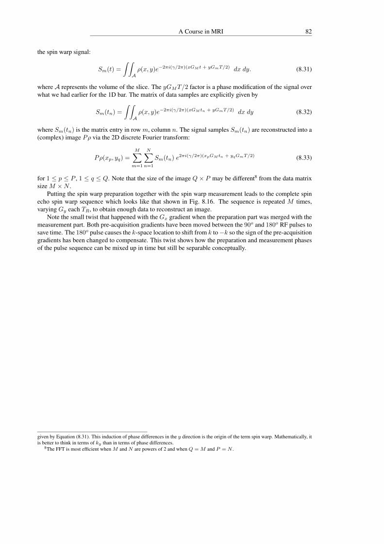
A Course in MRI 82
the spin warp signal:
Sm(t) =
∫ ∫Aρ(x, y)e−2πi(γ/2π)(xGM t + yGmT/2) dx dy. (8.31)
where A represents the volume of the slice. The yGMT/2 factor is a phase modification of the signal overwhat we had earlier for the 1D bar. The matrix of data samples are explicitly given by
Sm(tn) =
∫ ∫Aρ(x, y)e−2πi(γ/2π)(xGM tn + yGmT/2) dx dy (8.32)
where Sm(tn) is the matrix entry in row m, column n. The signal samples Sm(tn) are reconstructed into a(complex) image Pρ via the 2D discrete Fourier transform:
Pρ(xp, yq) =
M∑m=1
N∑n=1
Sm(tn) e2πi(γ/2π)(xpGM tn + yqGmT/2) (8.33)
for 1 ≤ p ≤ P , 1 ≤ q ≤ Q. Note that the size of the image Q× P may be different8 from the data matrixsize M ×N .
Putting the spin warp preparation together with the spin warp measurement leads to the complete spinecho spin warp sequence which looks like that shown in Fig. 8.16. The sequence is repeated M times,varying Gy each TR, to obtain enough data to reconstruct an image.
Note the small twist that happened with the Gx gradient when the preparation part was merged with themeasurement part. Both pre-acquisition gradients have been moved between the 90o and 180o RF pulses tosave time. The 180o pulse causes the k-space location to shift from k to−k so the sign of the pre-acquisitiongradients has been changed to compensate. This twist shows how the preparation and measurement phasesof the pulse sequence can be mixed up in time but still be separable conceptually.
given by Equation (8.31). This induction of phase differences in the y direction is the origin of the term spin warp. Mathematically, itis better to think in terms of ky than in terms of phase differences.
8The FFT is most efficient when M and N are powers of 2 and when Q = M and P = N .
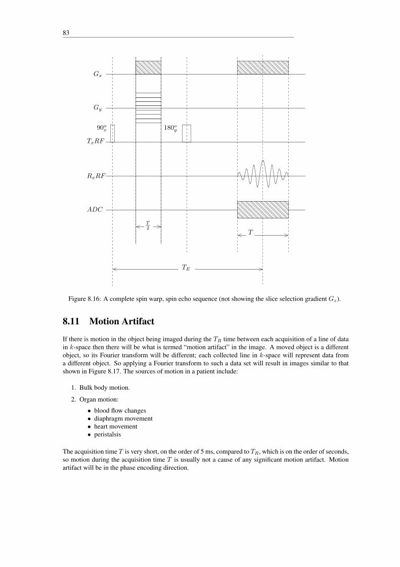
83
������������������������������������������������������������
������������������������������������������������������������
������������������������������������������������������������
������������������������������������������������������������
����������������
��������������������������������
������������������������
������������������������
90ox
T2
180oy
TE
T
Gx
Gy
TxRF
RxRF
ADC
Figure 8.16: A complete spin warp, spin echo sequence (not showing the slice selection gradient Gz).
8.11 Motion Artifact
If there is motion in the object being imaged during the TR time between each acquisition of a line of datain k-space then there will be what is termed “motion artifact” in the image. A moved object is a differentobject, so its Fourier transform will be different; each collected line in k-space will represent data froma different object. So applying a Fourier transform to such a data set will result in images similar to thatshown in Figure 8.17. The sources of motion in a patient include:
1. Bulk body motion.
2. Organ motion:
• blood flow changes• diaphragm movement• heart movement• peristalsis
The acquisition time T is very short, on the order of 5 ms, compared to TR, which is on the order of seconds,so motion during the acquisition time T is usually not a cause of any significant motion artifact. Motionartifact will be in the phase encoding direction.
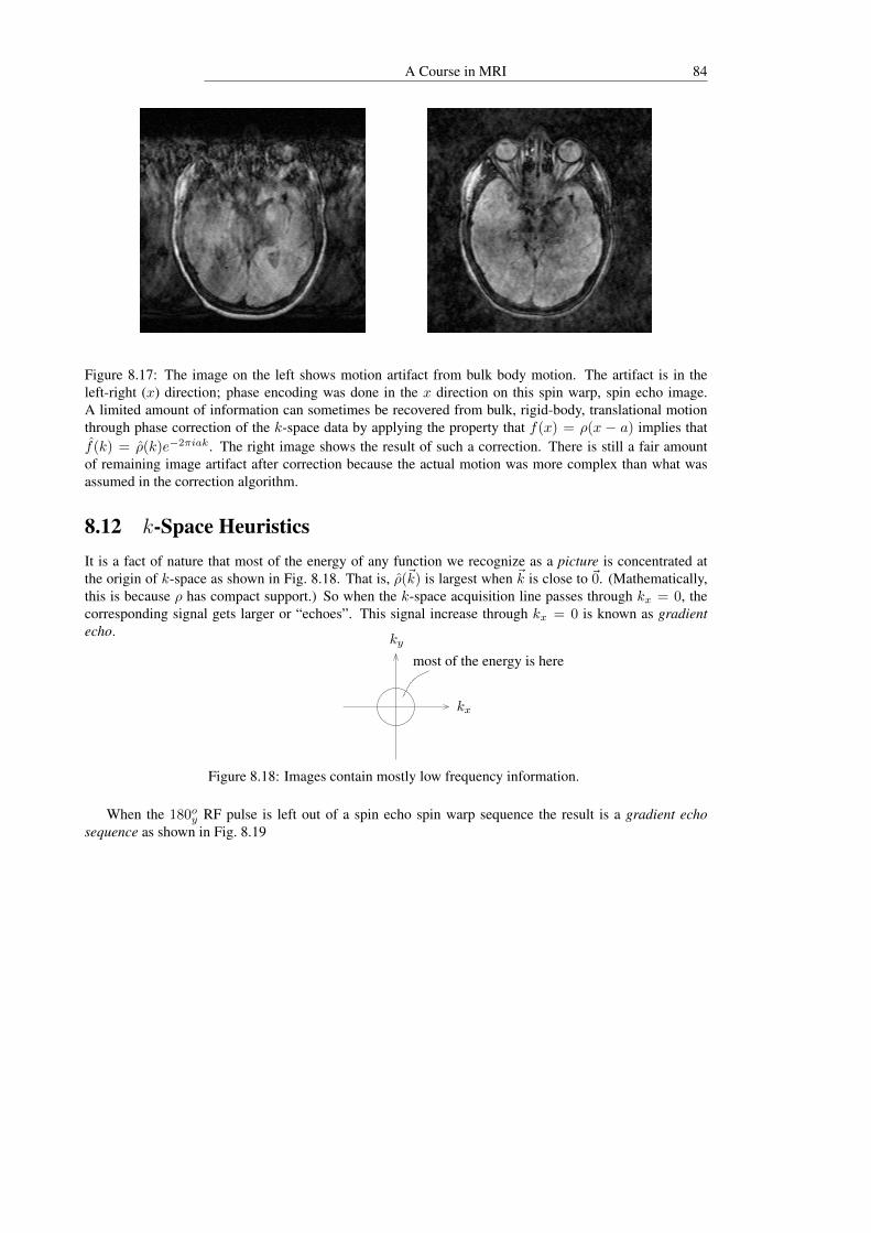
A Course in MRI 84
Figure 8.17: The image on the left shows motion artifact from bulk body motion. The artifact is in theleft-right (x) direction; phase encoding was done in the x direction on this spin warp, spin echo image.A limited amount of information can sometimes be recovered from bulk, rigid-body, translational motionthrough phase correction of the k-space data by applying the property that f(x) = ρ(x − a) implies thatf(k) = ρ(k)e−2πiak. The right image shows the result of such a correction. There is still a fair amountof remaining image artifact after correction because the actual motion was more complex than what wasassumed in the correction algorithm.
8.12 k-Space HeuristicsIt is a fact of nature that most of the energy of any function we recognize as a picture is concentrated atthe origin of k-space as shown in Fig. 8.18. That is, ρ(~k) is largest when ~k is close to ~0. (Mathematically,this is because ρ has compact support.) So when the k-space acquisition line passes through kx = 0, thecorresponding signal gets larger or “echoes”. This signal increase through kx = 0 is known as gradientecho.
ky
most of the energy is here
kx
Figure 8.18: Images contain mostly low frequency information.
When the 180oy RF pulse is left out of a spin echo spin warp sequence the result is a gradient echosequence as shown in Fig. 8.19

85
��������������������������������
����������������
��������������������������������
��������������������������������
������������������������������������������������������������
������������������������������������������������������������
������������������������������������������������������������
������������������������������������������������������������������������������������
������������������������
������������������������������������������
������ ������
Gx
Gy
TxRF
RxRF
ADC
90o
TE
T
Figure 8.19: Leaving out the 180◦ RF pulse give a “gradient echo” imaging sequence.
While a spin echo sequence produces T2 weighted image (Pρ ∼ ρe−TE/T2 ), a gradient echo sequenceproduces T ∗2 weighted images (Pρ ∼ ρe−TE/T∗2 ), when TR is long.
High spatial frequencies represent fine detail and low spatial frequencies (near ~K = ~0) represent coarsedetail (overall contrast) as illustrated in Fig. 8.20. So collecting data at a large k-space radius theoreticallywill increase resolution, the fact that the signal is lower there means that noise will eventually prevent thecollection of high spatial frequency information.
Some Terminology:
• ∆t = dwell time, time between samples (µs).
• Bw = γ2πGMV = bandwidth of acquisition (KHz). Bandwidth is important because the RF receiver
must be equally sensitive all the frequencies in the bandwidth. Sequence authors frequently report the“bandwidth per pixel” which is just Bw/P . Also, because of the way digital signals are processed, itis true that ∆t = 1
Bw.
Bandwidth and dwell time are parameters that you will encounter if you ever need to write pulse sequencesor have to evaluate the merits of pulse sequences. Note that the signal acquisition time may be derived fromthe bandwidth:
T = N∆t = N/Bw. (8.34)
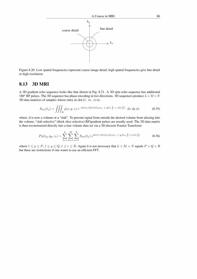
A Course in MRI 86
fine detailcoarse detail
ky
kx
Figure 8.20: Low spatial frequencies represent coarse image detail; high spatial frequencies give fine detailor high resolution.
8.13 3D MRIA 3D gradient echo sequence looks like that shown in Fig. 8.21. A 3D spin echo sequence has additional180o RF pulses. The 3D sequence has phase encoding in two directions. 3D sequences produce L×M×N3D data matrices of samples whose entry in slot (`, m, n) is:
S`m(tn) =
∫∫∫Aρ(x, y, z) e−2πi(γ/2π)(xGM tn + yGn
T2 + zG`
T2 ) dx dy dz (8.35)
where A is now a volume or a “slab”. To prevent signal from outside the desired volume from aliasing intothe volume, “slab selective” (thick slice selective) RF/gradient pulses are usually used. The 3D data matrixis then reconstructed directly into a true volume data set via a 3D discrete Fourier Transform:
Pρ(xp, yq, zr) =
L∑`=1
M∑m=1
N∑n=1
S`m(tn) e2πi(γ/2π)(xpGM tn + yqGmT2 +zrG`
T2 ) (8.36)
where 1 ≤ p ≤ P , 1 ≤ q ≤ Q, 1 ≤ r ≤ R. Again it is not necessary that L×M ×N equals P ×Q× Rbut there are restrictions if one wants to use an efficient FFT.
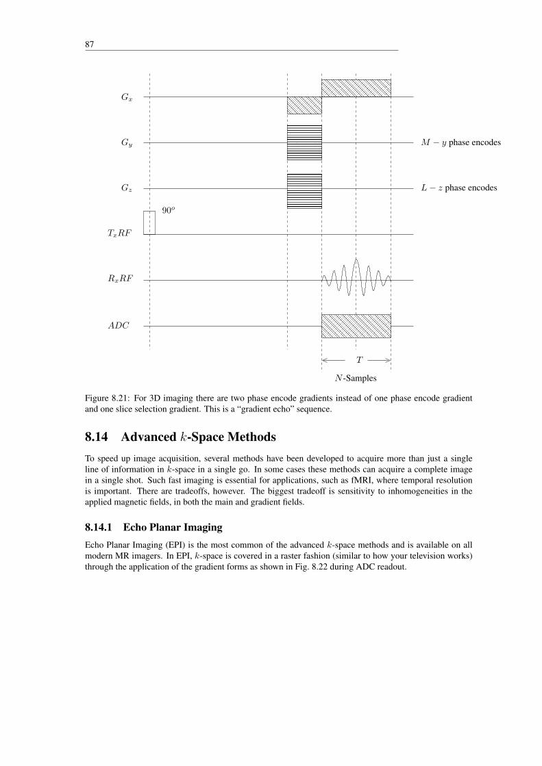
87
������������������������������������������������������������
������������������������������������������������������������
������������������������������������������������������������
������������������������������������������������������������
������������������������������������������������������������
��������������������������������
����������������
��������������������������������
��������������������������������
��������������������������������
��������������������������������
������������������������
������������������������
Gx
Gy
Gz
TxRF
RxRF
ADC
M − y phase encodes
L− z phase encodes
T
N -Samples
90o
Figure 8.21: For 3D imaging there are two phase encode gradients instead of one phase encode gradientand one slice selection gradient. This is a “gradient echo” sequence.
8.14 Advanced k-Space MethodsTo speed up image acquisition, several methods have been developed to acquire more than just a singleline of information in k-space in a single go. In some cases these methods can acquire a complete imagein a single shot. Such fast imaging is essential for applications, such as fMRI, where temporal resolutionis important. There are tradeoffs, however. The biggest tradeoff is sensitivity to inhomogeneities in theapplied magnetic fields, in both the main and gradient fields.
8.14.1 Echo Planar ImagingEcho Planar Imaging (EPI) is the most common of the advanced k-space methods and is available on allmodern MR imagers. In EPI, k-space is covered in a raster fashion (similar to how your television works)through the application of the gradient forms as shown in Fig. 8.22 during ADC readout.

A Course in MRI 88
k y
k x
t
...
...
Gx
Gy
t
No signal collection
Figure 8.22: Rapid switching of the gradients in EPI enables one to sample all of k-space in one-shot.
8.14.2 SpiralThe next most common advanced k-space method after EPI is the spiral. Currently spiral is an experimentalmethod and is not yet standardly available on commercial MR equipment. In spiral imaging, k-space iscovered in a spiral fashion through the application of the following gradient forms during ADC readout asshown in Fig. 8.23.
0.2 0.4 0.6 0.8 1
-1000
-500
500
1000
0.2 0.4 0.6 0.8 1
-1000
-500
500
1000
-10 10 20
-20
-15
-10
-5
5
10
15
t
t
Gy
Gxky
kx
Figure 8.23: k-space can be covered in a spiral fashion with oscillating gradients of increasing amplitude.Starting the data acquisition at the center of k-space makes the image less susceptible to motion artifacts.

89
8.14.3 STAR (Single TrAjectory Radial) AcquisitionThe STAR is my invention and has yet to find a niche application. In STAR imaging, k-space is covered ina spiral fashion through the application of the gradient forms during ADC readout as shown in Fig. 8.24.
Figure 8.24: STAR imaging scheme. (The gradient waveform image is taken from a software implementa-tion on an old Siemens MRI.)
The spiral, and to a lesser extent, the STAR, have the advantage over EPI of starting data acquisitionat the origin of k-space. This reduces the effective TE . Also the radial nature of the acquisition reducesmotion artifact in the reconstructed image.
8.14.4 Rosette and Lissajous ImagingThese two methods are useful for spectroscopic imaging (see Chapter 13) because off-resonance signals“blur out”. Therefore one can reconstruct at a predefined chemical shift and get a sharp image from onlythe frequency of interest.
In rosette and Lissajous imaging, k-space is covered in the fashion shown in Fig.8.25.
−600 −400 −200 0 200 400 600
−600
−400
−200
0
200
400
600
-20 -10 10 20kx
-20
-10
10
20
ky
Rosette Lissajous
Figure 8.25: There are many ways to travel through k-space, based on Equation (8.29).
The gradient waveforms required for rosette imaging are sums of two sine waves at slightly different fre-quencies. The gradient waveforms required for Lissajous imaging are two sine waves, one for Gx and onefor Gy , that are at different frequencies and out of phase with each other.

A Course in MRI 90
Exercises1. Referring to Equation (8.2), write the real and imaginary parts of f if f is complex-valued. That is,
if f = fR + ifI .
2. *Show that the integral Fourier transform of the boxcar function is a sinc function. Hint: computef(k) =
∫ A−A e
−2πikxdx.
3. If, in a 1D imaging situation similar to that covered in Sections 8.7 and 8.9, the bar was 100mm longand we wanted to image it in 5ms with a resolution of 256 pixels, what gradient strength is required?(State your answer in mT/meter.)
4. Derive Equation (8.30) explicitly. Use t0 = −T and tI = −T2 . What is k0?
5. Show that the Nyquist criterion of ∆k = 1V is equivalent to ∆t = 1
Bw.
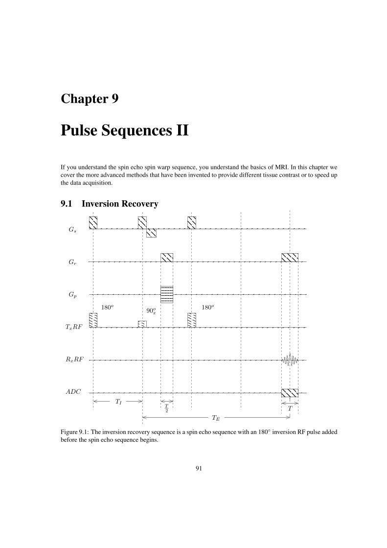
Chapter 9
Pulse Sequences II
If you understand the spin echo spin warp sequence, you understand the basics of MRI. In this chapter wecover the more advanced methods that have been invented to provide different tissue contrast or to speed upthe data acquisition.
9.1 Inversion Recovery
Gs
Gr
Gp
TxRF
RxRF
ADC
180o90ox
180o
TIT2
TE
T
Figure 9.1: The inversion recovery sequence is a spin echo sequence with an 180◦ inversion RF pulse addedbefore the spin echo sequence begins.
91

A Course in MRI 92
Besides the spin echo sequence, another relatively common sequence is the inversion recovery sequenceshown above. The inversion recovery sequence existed for NMR in the days before imaging because itwas useful for bulk T1 measurement. The sequence is actually obtained through the minor modification ofadding a 180o RF pulse at the beginning of a spin echo sequence. In the timing diagram above, we haveused Gs, Gr, and Gp for slice, read and phase gradients instead of our usual Gx, Gy , Gz to reflect the factthat the relevant coordinates are on the slice.
The inversion recovery sequence has an extra parameter, TI , the inversion time to add to TR and TE . Byremoving the second 180o RF pulse and sliding the two gradient pieces together, a gradient echo version ofthe inversion recovery sequence is possible.
In terms of rotating frame cartoons the effect of the 180o inversion pluse is as shown in Figures 9.2.
z
y
x
M0
just before 180o pulse
z
y
x
−M0
just after 180o pulse
Figure 9.2: Spin cartoon showing the effect of the 180◦ inversion RF pulse.
At TI one of three cases can happen, as shown in Figure 9.3, depending on the value of T1.case 1
long T1
z
y
x
case 2
2e−TIT1 = 1
z
y
x
case 3
Short T1
z
y
x
Figure 9.3: The longitudinal magnetization available after TI depends on the value of T1 of the object beingimaged.

93
Then, after the 90o pulse we get the situation as shown in Figure 9.4.case 1
z
y
x
A “negative” transversemagnetization if T1 is long.[Real, as opposed to modulus,reconstruction can recover thisnegativeness.]
case 2z
y
x
Nothing if e−TIT1 = 1
2 .
case 3z
y
x
A transverse magnetizationless than M0 if T1 is short.
Figure 9.4: The transverse magnetization produced after the 90◦ RF pulse in an inversion recovery sequencedepends on the value of T1.
This behavior is due to the solution of the Bloch equation as shown in Figure 9.5.
Mz
M0
−M0
t = 0case
1 2 3
Differentchoices for
TI
Figure 9.5: The longitudinal magnetization available before the 90◦ RF pulse depends on the relative mag-nitudes of TI and T1. The time t = 0 here is the time just after the 180◦ inversion RF pulse.
The zero crossing of the recovery curve means that the signal from a selected tissue, like fat, can bemade equal to zero and eliminated from the image. The sequence also gives more dynamic range than theregular spin echo sequence; from −M0 to +M0 instead of from 0 to +M0.

A Course in MRI 94
9.2 Turbo Spin Echo: Speeding up the data acquisitionBy modifying the multiple echo T2 sequence with the addition of phase gradients, a bunch, say F , ofk-space lines can be collected in one TR.
��������
������������
������������
������������
����
������������
������������
������
������
������
������
������
������
������
������
������������������������������������������������������������������������������������������������
����������������
��������
�������� ��
������
������
������
������
������
������
������
������
������
TE TE TE TE
Gs
Gr
Gp
TxRF
RxRF
ADC
90ox 180oy 180oy 180oy 180oy
Figure 9.6: Using a different amplitude for the phase gradient for each echo in a multiple echo T2 sequencegives multiple lines in k-space. Such a sequence is called “turbo spin echo” by Siemens and ”fast spinecho” (FSE) by General Electric.
In the example shown in Figure 9.6, F = 4 is the “turbo factor”. With this sequence the data acquisitionis sped up by F = 4 times. That is, F = 4 lines in k-space are acquired where normally only one linewould be collected. But each line is collected at a different TE . The effective TE is that experienced by thecentral k-space lines (which define the contrast). So one strategy is to collect a central k-space line at thefirst TE and use the other echos to collect the higher frequency k-space lines. Then the effective TE is thefirst TE for the central k-space line.
To compute the imaging time for a particular generic sequence, compute:
Tim =N · TR ·Av
F
where
N = number of phase space lines,
TR = repeat time,
Av = number of signal averages, used to reduce noise,
F = “turbo factor” = 1 for ordinary sequences.
The maximum number of slices, S, that can be obtained in a single TR is
S <TR
FTE + TI.

95
9.3 Using the Steady State to Speed up MRI data acquisition
The problem with the SE approach to MRI is the long TR required between each k-space line acquisition.It would be nice to be able to reduce TR to the 10 to 30 ms range. Setting up a steady state magnetizationin the presence of a long string of RF and gradient pulses provides a way of drastically reduing the TR.Speeding up the acquisition through the use of gradient echos from magnetization in a steady state makes3D MRI practical.
If we combine TxRF , RxRF and Gr of the timing diagram into one line, the basic approach to steadystate imaging is given by the scheme shown in Figure 9.7.
θ θ θ θ θ θ θ
α α α α α α
Repeated RF pulses with α tip angle
FID ECHO
Gr that producean overall phase dispersionof the transverse magnetizationof θ degrees.
Figure 9.7: Steady state sequences are composed of a mix of RF and gradient pulses.
Two types of received RF signal are created:
1. The FID just after the α RF pulse.
2. The ECHO just before the α RF pulse.
In NMR, FID stands for Free Induction Decay and refers to transverse magnetization that is produced,and decays, just after rotating magnetization into the transverse plane with an RF pulse. Here we call thesignal just after an α RF pulse an FID because it will contain the influences of all the α pulses that occurredbefore, and the influence of the ECHO signal from just before the α RF pulse. But, primarily, the behaviorof the FID is like a simple fid and will be influenced largely by T1 effects because it will be caused bylongitudinal magnetization that has just been tipped into the transverse plane.
The ECHO has its primary influence the echo from two α RF pulses ago. The echo is the spin echocaused by a sequence of two α pulses. In this case a dispersion of θ degrees is deliberately caused in thetransverse magnetization by essentially always having the gradients turned on. Note that a regular spin echois caused by a 90o – 180o RF pulse sequence. This is just the most efficient way of producing a spin echo.You still get echoes from an α – α RF pulse sequence. The ECHO is caused, in total, by all the previouspulse sequence activity.
The idea with steady-state is to allow the periodic sequence of RF and gradient pulses to run for a periodof time so that the FID and ECHO signals are the same for each repetition. When this occurs, a steady statemagnetization has been achieved.
It is very difficult to try and deduce what the steady state will be if you try to follow the individual αRF and θ gradient pulses and what they do to relaxing magnetization. Fortunately, it is relatively straightforward to figure out what the steady state will be mathematically. In what follows we will only give theresults of the steady state computations.
To get an image from the steady state approach, the gradient must have a shape conducive to k-spaceencoding. Then we have a choice of making an image from either the FID or the ECHO.
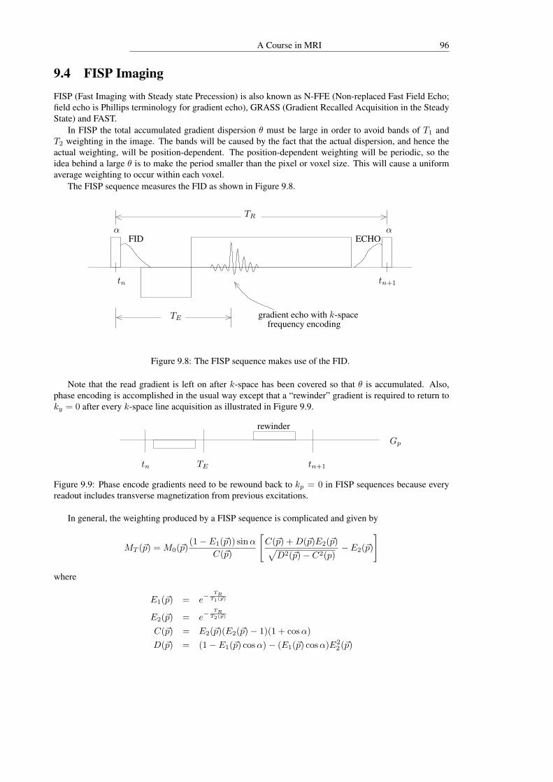
A Course in MRI 96
9.4 FISP Imaging
FISP (Fast Imaging with Steady state Precession) is also known as N-FFE (Non-replaced Fast Field Echo;field echo is Phillips terminology for gradient echo), GRASS (Gradient Recalled Acquisition in the SteadyState) and FAST.
In FISP the total accumulated gradient dispersion θ must be large in order to avoid bands of T1 andT2 weighting in the image. The bands will be caused by the fact that the actual dispersion, and hence theactual weighting, will be position-dependent. The position-dependent weighting will be periodic, so theidea behind a large θ is to make the period smaller than the pixel or voxel size. This will cause a uniformaverage weighting to occur within each voxel.
The FISP sequence measures the FID as shown in Figure 9.8.
TR
α αFID ECHO
tn tn+1
TE gradient echo with k-spacefrequency encoding
Figure 9.8: The FISP sequence makes use of the FID.
Note that the read gradient is left on after k-space has been covered so that θ is accumulated. Also,phase encoding is accomplished in the usual way except that a “rewinder” gradient is required to return toky = 0 after every k-space line acquisition as illustrated in Figure 9.9.
tn TE tn+1
rewinder
Gp
Figure 9.9: Phase encode gradients need to be rewound back to kp = 0 in FISP sequences because everyreadout includes transverse magnetization from previous excitations.
In general, the weighting produced by a FISP sequence is complicated and given by
MT (~p) = M0(~p)(1− E1(~p)) sinα
C(~p)
[C(~p) +D(~p)E2(~p)√D2(~p)− C2(p)
− E2(~p)
]
where
E1(~p) = e− TRT1(~p)
E2(~p) = e− TRT2(~p)
C(~p) = E2(~p)(E2(~p)− 1)(1 + cosα)
D(~p) = (1− E1(~p) cosα)− (E1(~p) cosα)E22(~p)

97
But, if TR << T2 and α >> αE where αE is the “Ernst angle” (defined later) then this simplifies to
MT (~p) = M0(~p)sinα
1− cosα
T2(p)
2T1(p)
so that FISP gives a T2/T1 contrast.
9.5 PSIF ImagingPSIF measures the ECHO and looks like a “time-reversed” FISP:
TR
TE
FID ECHO
tn tn+1
PSIF gradient echo with k-space frequency encoding
Figure 9.10: The PSIF sequence makes use of the ECHO.
Again, the contrast from PSIF, which must also have large θ, is complicated in general:
MT (~p) = M0(~p)(1− E1(~p))E2(~p)
C(~p)sinα
(1− D(~p) + C(~p)E2(~p)√
D2(~p)− C2(~p)
)
When TR is short and α >> αE PSIF also tends to produce T2
T1constrast images.
9.6 “True FISP” ImagingBy setting the gradient pulses up so that θ = 0, the contrast banding problem can be avoided and thegradient echo associated with the FID and the ECHO will be identical. This sequence is called “true FISP”.True FISP is very sensitive to flow with slow flow material (e.g. CSF) appearing brighter than fast flowmaterial (e.g. blood).

A Course in MRI 98
9.7 FLASH ImagingBy cycling the phase of the α RF pulses, as shown in Figure 9.11, the ECHO can be destroyed or “spoiled”leaving only a T1 weighted FID signal. Such “RF spoiled” steady state sequences are called FLASH(FastLow Angle SHot) sequences.
z
x
y
α
phase = 0◦
B1 axis
z
x
y
α
60o
phase = 60◦
B1 axis
z
x
y
α
120o
phase = 120◦
B1 axis
Figure 9.11: FLASH works similarly to FISP except that the phase of the α RF pulse is cycled througha series of angles, each one 60◦ more than the previous excitation in the sequence illustrated here. Thetipping angle α is in the plane perpendicular to ~B1.
With FLASH (or any other T1 sequence) the maximum signal is obtained at the Ernst angle αE givenby:
cosαE = e−TR/T1
Tissues whose T1 gives an Ernst angle that matches the tip angle of the sequence will be brightest in theimage.
9.8 Transient State ImagingThe steady state approach requires a few cycles of α and θ pulses to pass before the steady state is reached.The period before steady state is a transient state in which the contrast (weighting) after every excitation isdifferent.
Images can be made during the transient phase if the sequence is set up so that the central k-space linesend up with the overall weighting desired. this is exactly what was done with TSE (turbo spin echo) inselecting an effective TE .
With transient imaging, the state of magnetization can be “prepared” before the train of α and θ pulsesbegin. Such preparation and transient phase measurement leads to images that have contrast or weightingthat is impossible to obtain with steady state imaging. The most widely used “magnetization preparation”used is the addition of a 180o RF inversion pulse before the α, θ train. This leads to the enhanced T1 inver-sion recovery contrast that is useful, for example, for differentiating fine structures around the hippocampus.
The MP-RAGE (Magnetization Prepared - RApid Gradient Echo) is an example of an inversion recoverytransient state imaging sequence.
9.9 Using the Ernst AngleWhen using the steady state or transient state FFE imaging methods there is a trade-off between speed andsignal-to-noise ratios (SNR). A larger flip angle α will give a higher SNR because it flips more longitudinalmagnetization into the transverse plane. But larger α means that TR will have to be longer to obtain thesame T1 constrast. This reasoning applies mostly to FLASH type imaging but also applies to SE imagingwhere an α pulse is used in place of a 90o pulse.

99
So suppose you have sequence A with αA and TRA and a sequence B with αB and TRB . If we want animage with the same T1 contrast, αA and TRA must have specific relationships to αB and TRB . To find therelationships, assume that αA, TRA and αB , TRB correspond to the T1 tissue that produces the brightestgrey-scale value. In other words, αA and αB are both Ernst angles for that tissue. So
cosαA = e−TRA/T1 and cosαB = e−TRB /T1
Solving for T1 gives
T1 =−TRA
ln(cosαA)=
−TRBln(cosαB)
.
Suppose we are given αA, TRA and αB then the TRB required to have the same T1 contrast in bothsequences is:
TRB = TRAln(cosαB)
ln(cosαA).
If we have αA, TRA and TRB then the αB to have the same T1 contrast in both sequences is:
αB = arccos[eln(cosαA)TRB /TRA
].
9.10 Diffusion ImagingIf, in the rotating frame, we write the transverse magnetization as a complex number:
MT (~p, t) = Mx(~p, t) + iMy(~p, t)
then we can write the Bloch equation for the transverse magnetization as one complex equation:
dMT
dt(~p, t) = −iγ ~G · ~p MT (~p, t)− MT (~p, t)
T2(~p). (9.1)
Equation (9.1) describes what happens ifMT (~p) doesn’t move. With diffusion (and flow) the magnetizationmoves around (the water molecules diffuse through tissues). To account for the motion, an extra term mustbe added to Equation (9.1). The extra term summarizes the net “diffusive” flux of MT and, if we onlyconsider diffusion in the z direction, the extra term is
Da∂2MT
∂z2(~p, t)
where Da is the apparent diffusion coefficient. So Equation (9.1) becomes
∂MT
∂t(~p, t) = −iγ ~G · ~p MT (~p, t)− MT (~p, t)
T2(~p)+Da
∂2MT
∂z2(~p, t). (9.2)
The solution to Equation (9.2), assuming that ~G = Gz , is
MT (~p, t) = MT (~p, 0) exp
[−Daγ
2
∫ t
0
(∫ τ
0
Gz(ζ)dζ
)2
dτ
]exp
[−iγz
∫ t
0
Gz(τ)dτ − t
T2
]The second exponential term describes T2 relaxation and precession under the gradients. The first
exponential term gives diffusion weighting. The idea is to set up the gradients during preparation so that∫ TE
0
Gz(t) dt = 0.

A Course in MRI 100
Then the second exponential term will only give T2 weighting at t = TE and the first exponential termbecomes
exp
[−Daγ
2
∫ TE
0
(∫ τ
0
Gz(ζ)dζ
)2
dτ
]at t = TE . Let
b = γ2
∫ TE
0
(∫ τ
0
Gz(ζ)dζ
)2
dτ. (9.3)
Then the solution to Equation (9.2) is
MT (~p, t) = MT (~p, 0) e−bDa e−TE/T2 .
The term e−bDa adds diffusion weighting to the transverse magnetization and the term e−TE/T2 adds theusual T2 weighting.
The MR image is made sensitive to diffusion by adding gradients during the preparation stage. Theusual gradients added are bipolar gradients that look like those shown in Figure 9.12.
Gz
δ
∆
δ
t
Figure 9.12: Timing diagram for bipolar diffusion gradients.
It is easy to see that∫ TE
0Gzdt = 0 for bipolar gradients and that
b = γ2δ2
(∆− 1
3δ
)G2z (9.4)

101
So, a diffusion weighted spin echo sequence will look like that shown in Figure 9.13.
��������������������������������������������������
��������������������������������������������������
��������������������������������������������������
��������������������������������������������������
��������������������������������������������������
��������������������������������������������������
��������������������������������������������������������������
������������
Gz
Gs
Gr
Gp
TxRF
RxRF
ADC
δ δ
∆
90ox 180o
TE
Figure 9.13: Bipolar diffusion gradients inserted into a spin echo sequence.
In the timing diagram of Figure 9.13, note thatGz is used to show the diffusion gradients for z-directiondiffusion sensitivity andGs,Gr andGp are used for slice, read and phase gradients. Keep in mind, however,that Gs, Gr and Gp are physically functions of Gx, Gy and Gz .
The requirement that TE > ∆ means that diffusion images will always have T2 weighting along withthe diffusion weighting.
The effect of the diffusion gradients is to attenuate the T2-weighted image by a factor of e−bDa . Thatis, an attenuation of A is accomplished with
(1−A) = e−bDa (9.5)
Equation 9.5 is useful for determining what b needs to be for a given attenuation:
b = − ln(1−A)/Da.
Example. At room temperature, the diffusion coefficient for water is approximately D = 2.2 ×10⁻⁹ m2/s. So to achieve an attenuation of 10% we need b = − ln(0.9)/2.2 × 10−9 m2/s = 4.789 ×10⁷ s/m2. Suppose TE = 40 ms so that δ = 10 ms, ∆ = 15 ms are possible. Then with bipolar gradients,

A Course in MRI 102
Equation (9.4) gives
Gz =
√b
γ2δ2(∆− 13δ)
=
√4.789× 10⁷ s/m2
(2.68× 10⁸ T−1)2 × (0.01 s)2 ×(0.015− 0.01
3
)s
= 0.0239 T/m = 23.9 mT/m.
Which is quite large! This is typical of diffusion imaging requirements.Note that perfect bipolar gradients are not possible because it takes some time to build up current in the
gradient coils. In addition to a maximum gradient strength, an MRI will also have a maxium gradient slewrate (mT/m/s) that limits how fast the gradients can rise. So instead of ideal rectangular gradient profiles,the profiles will be trapezoidal. The bipolar gradients will really look like that shown in Figure 9.14.
risetime
falltime.
there is a and a
Figure 9.14: Real gradient pulses have to be ramped up and down.
A more accurate computation of b needs to take into account the trapezoidal shape of the gradient when∫ TE0
G(t) dt is calculated. Nevertheless, Equation (9.4) for b is still a good approximation because the riseand fall times will be small compared to δ.
Exercises
1. In an inversion recovery sequence, show that the longitudinal magnetization equals zero when 2e−TIT1 =
1. Use the longitudinal Bloch equation.
2. How long does it take to acquire an ordinary spin echo T1 weighted image with TR = 400 ms,TE = 15 ms, an acquisition matrix of 256×256 and 2 signal averages? If a turbo spin echo sequencethat collects 4 k-space lines at a go is used, what is acquisition time for the same T1-weighted image?How many slices can be obtained in each case?
3. Suppose a FLASH sequence with α = 10o and TR = 40 ms give the right image contrast that youwanted but the SNR was too low (the image is too grainy). You want to increase the SNR by doublingα to 20o. If you do that, what TR is required for the new imaging sequence? If the data matrix is256 × 256 × 64 (a 3D sequence) and 1 signal average is used, how long does it take to acquire theMRI data using the first sequence? How long for the second sequence? How long will it take toacquire the data for the first sequence by doubling the number of signal acquisitions? If acquisitiontime was important, which approach would you use to improve the SNR, increasing α or increasingthe number of signal averages?
4. *Using Equation 9.3, show that b for bipolar gradients is as given in Equation 9.4. (The derivation islong but straightforward.)

103
5. Suppose our MRI limits us to 10 mT/m maximum gradient strength. Assuming that δ = 10 ms and∆ = 15 ms what are b and the attenuation factor A?

A Course in MRI 104

Chapter 10
TRASE Imaging
In Chapter 8 we showed how to encode image information into the MRI signal by using B0 magnetic fieldgradients. The hardware, the gradient coil set, needed to create theB0 magnetic field gradients is significant,especially when they are required to be switched rapidly in EPI sequences. Gradient coils, and the powerelectronics feeding them, are required to handle current changes of hundreds of amps in under a millisecond.If we could encode image information into the NMR signal without expensive gradient hardware thenMRI could become a much more accessible medical imaging modality. Without gradient coils, imageinformation would need to be encoded through manipulation of the RF transmission. Two methods ofdoing this have emerged since the invention of MRI. They are 1. Rotating frame zeugmatography [11] and2. TRansmit Array Spatial Encoding (TRASE) [12, 19, 20]. In turns out that rotating frame zeugmatographyrequires too much RF energy from the point of view of Specific Absorption Rate (SAR) for it to be useful.SAR is a measure of how much RF energy is absorbed by the patient being imaged; if it is too high,the patient’s temperature increases. We will not cover rotating frame zeugmatography here. The TRASEmethod has much lower SAR and is a very promising method for future MRI. The basic Idea behind TRASEis that instead of using gradient magnetic fields, we use spatial phase variation in the RF transmission toencode spatial information in the NMR signal.
To make TRASE work we have to understand how accomplish two objectives:
1. How to create a spatially varying RF phase.
2. How to use the NMR signal created by a TRASE RF coil to reconstruct an image.
We will consider each aspect of TRASE in turn.
10.1 TRASE RF CoilsAssuming that the main magnetic field ~B0 is in the z direction, ~k, the three required TRASE ~B1 fields inthe rotating frame are given by
~B1x = B1
[sin(Gxx)~i+ cos(Gxx)~j
](10.1)
~B1y = B1
[sin(Gyy)~i+ cos(Gyy)~j
](10.2)
~B1z = B1
[sin(Gzz)~i+ cos(Gzz)~j
]. (10.3)
Equations (10.1), (10.2), and (10.3) describe ~B1 fields with phase gradients, of magnitudeGi (radians/meter),in the x, y, and z directions respectively. (Of course, a constant phase can be added to these expressions.)Figures 10.1 and 10.2 illustrate the B1 fields of Equations (10.1) and (10.2).
105

A Course in MRI 106
Figure 10.1: TRASE B1 field in the x direction as given by Equation (10.1).
Figure 10.2: TRASE B1 field in the y direction as given by Equation (10.2).
Figures 10.3 and 10.4 show some ways that the ideal TRASE fields may be obtained, to a level ofapproximation that is useful for producing images. Of these cases, the spiral birdcage design is the easiestto understand, see Figure 10.5. The regular birdcage coil gives a good engineering approximation of sheetof cylindrical current density flowing in the z (cylinder axis) direction. The continuous case produces auniformB1 field (in the rotating frame) inside the cylinder if the current varies sinusoidally in the cylindricalangular direction. The birdcage coil, with a finite number of conductors instead of a continuous cylindricalsurface, produces a practically uniform B1 field inside the coil. By twisting the birdcage coil, the B1 fieldwill be given a phase variation in the z direction.
Figure 10.3: Illustrated here are two ways to build an RF coil to produce TRASE ~B1 phase gradient fieldsin the x and y directions, assuming that ~B0 is in the z direction. A combination of Maxwell and Helmholtzcoil pairs are used. These images are taken from [19].

107
Figure 10.4: Illustrated here are two ways to build an RF coil to produce TRASE ~B1 phase gradient fields inthe z direction, assuming that ~B0 is in the z direction. On the left is shown a spiral birdcage RF coil whosez direction is along the cylindrical axis of the coil. On the right, a combination large and small Helmholtzcoil pairs are used. These images are taken from [12].
Figure 10.5: Twisting a regular birdcage coil is one way to produce a B1 field with a phase variation alongthe cylindrical z direction.
10.2 How to use a TRASE NMR signal to reconstruct an image
10.2.1 k-space origin of a TRASE coil
As with B0 gradient fields, more than one TRASE RF coil may be used at the same time. So it is useful todefine a TRASE phase gradient vector ~G = Gx~i + Gy~j + Gz~k. With ~p = x~i + y~j + z~k, the transversecomponents of the ~B1 field (the x and y components of ~B1 perpendicular to ~B0) may be described by acomplex number B1 as follows:
B1(~p) = |B1|(~p)eiΦ(~p) = |B1|(~p)ei~G·~p = |B1|(~p)e2πi~k·~p = B1x(~p) + iB1y(~p) (10.4)
where ~k = ~G/2π, Φ(~p) = ~G.~p is the transverse B1 phase at ~p and |B1|(~p) =√B2
1x(~p) +B21y(~p) is
the transverse magnitude of B1. Do not confuse B1x and B1y in Equation (10.4) with ~B1x and ~B1y inEquations (10.1) and (10.2).
To fix ideas, set ~G = (1, 0, 0) (using row vector notation) and consider the effect of a 90◦ TRASE
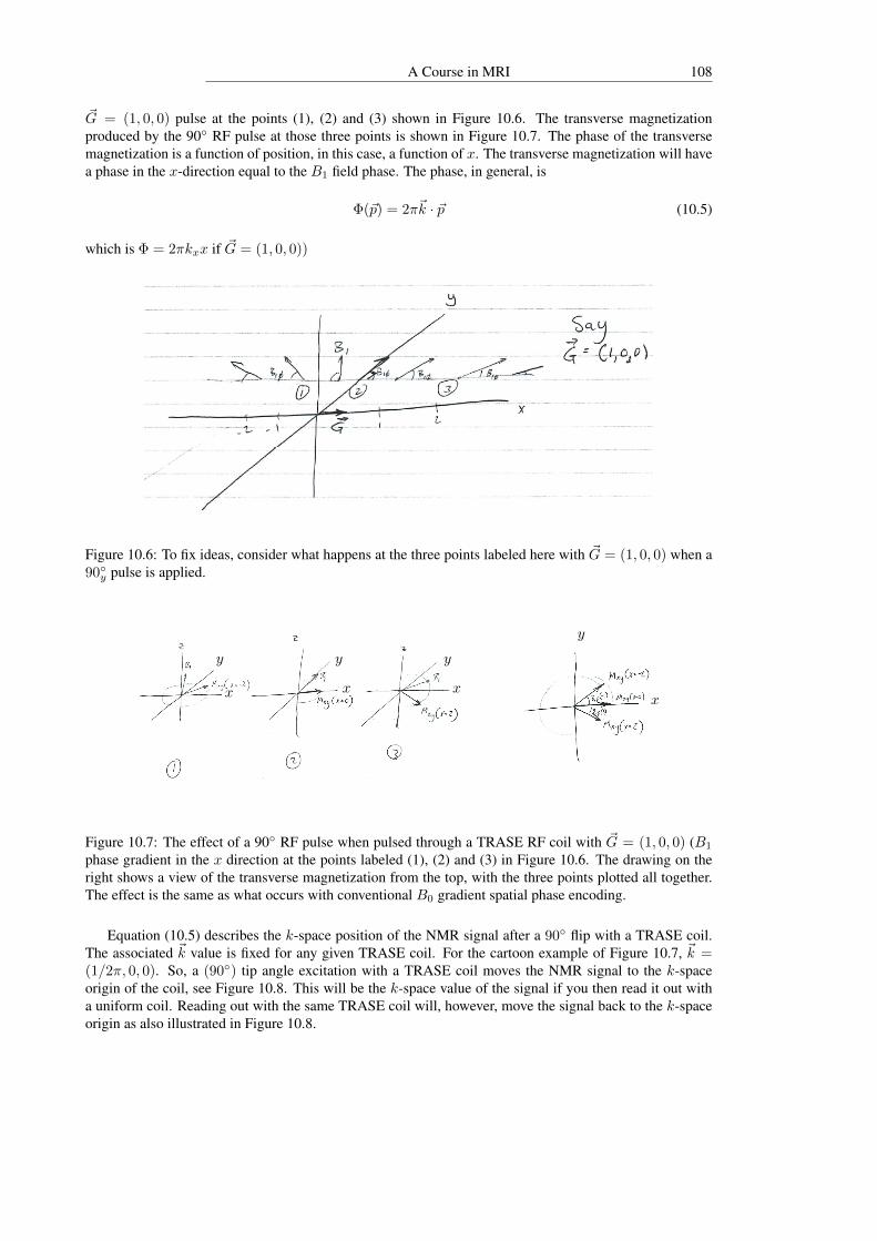
A Course in MRI 108
~G = (1, 0, 0) pulse at the points (1), (2) and (3) shown in Figure 10.6. The transverse magnetizationproduced by the 90◦ RF pulse at those three points is shown in Figure 10.7. The phase of the transversemagnetization is a function of position, in this case, a function of x. The transverse magnetization will havea phase in the x-direction equal to the B1 field phase. The phase, in general, is
Φ(~p) = 2π~k · ~p (10.5)
which is Φ = 2πkxx if ~G = (1, 0, 0))
Figure 10.6: To fix ideas, consider what happens at the three points labeled here with ~G = (1, 0, 0) when a90◦y pulse is applied.
x x xx
y y y
y
Figure 10.7: The effect of a 90◦ RF pulse when pulsed through a TRASE RF coil with ~G = (1, 0, 0) (B1
phase gradient in the x direction at the points labeled (1), (2) and (3) in Figure 10.6. The drawing on theright shows a view of the transverse magnetization from the top, with the three points plotted all together.The effect is the same as what occurs with conventional B0 gradient spatial phase encoding.
Equation (10.5) describes the k-space position of the NMR signal after a 90◦ flip with a TRASE coil.The associated ~k value is fixed for any given TRASE coil. For the cartoon example of Figure 10.7, ~k =(1/2π, 0, 0). So, a (90◦) tip angle excitation with a TRASE coil moves the NMR signal to the k-spaceorigin of the coil, see Figure 10.8. This will be the k-space value of the signal if you then read it out witha uniform coil. Reading out with the same TRASE coil will, however, move the signal back to the k-spaceorigin as also illustrated in Figure 10.8.

109
Figure 10.8: Left: A 90◦ RF pulse applied through a TRASE coil moves the NMR signal to the k-spaceorigin of the coil. Right: If you read out that signal with the same TRASE coil without further RF manipu-lation, the NMR signal will be rephased to the origin of k-space.
10.2.2 TRASE imaging pulse sequencesThe RF manipulation that we must do to avoid rephasing the NMR signal back to the k-space origin andalso to move the signal to other locations in k-space different from the TRASE coil’s k-space origin is touse a series of 180◦ RF pulses. So let’s examine the effect of a series of 180◦ RF TRASE pulses. Writetransverse magnetization as a complex number:
Mxy = Mx + iMy. (10.6)
Let M−xy be the transverse magnetization just before the 180◦ TRASE RF pulse and M+xy be the transverse
magnetization just after the 180◦ TRASE RF pulse.We will be considering the effect of two TRASE coils, A and B, each with their own K-space origins,
~kA and ~KB . These k-space origins correspond to the position dependent phase angles:
ΦA(~p) = 2π~kA · ~p (10.7)
andΦB(~p) = 2π~kB · ~p. (10.8)
The effect of a 180◦ TRASE RF pulse is
M+xy(~p) = M−xy(~p) ei2Φ(~p) (10.9)
where M−xy is the complex conjugate of M−xy . See Figure 10.9 for a derivation of Equation (10.9).
~B1~B1
M−xy
M+xy
x x
y y
Figure 10.9: The origin of the complex conjugate and the factor of 2 in the phase of Equation (10.9).Let M−xy = Meiα and let Φ be the angle that ~B1 makes with the x axis – the phase of ~B1. So theangle between the ~B1 direction and the Mxy direction, both before and after the flip is Φ − α. ThenM+xy = Mei(Φ+[Φ−α]) = Me−iαei2Φ = M−xy ei2Φ.

A Course in MRI 110
Measurement with the A TRASE coil results in
Mmeas(~p) = Mactual(~p)e−iΦA(~p) (10.10)
as per the situation shown in Figure 10.8.Now let’s consider the sequence shown in Figure 10.10.
Figure 10.10: A TRASE imaging sequence. A labels RF pulses through the coil with k-space origin kAand B labels RF pulses through the coil with k-space origin kB . The Mi denote measurements with the Acoil.
Adopting the convention that ~B1 is along the y axis at ~p = 0, the first 90◦ TRASE RF pulse at thebeginning of the sequence shown in Figure 10.10, from the TRASE coil with k-space origin ~kA, results inthe transverse magnetization:
Mxy = M0 eiΦA (10.11)
where ΦA = ~GA · ~p = 2π ~kA · ~p. To fix ideas with a concrete example, let ~kA = (1/4, 0, 0) and ~kB =(−1/4, 0, 0) and let
• 90i denote a 90◦ flip with TRASE coil i; this is governed by Equation (10.11).
• 180i denote 180◦ flip with TRASE coil i; this is governed by Equation (10.9).
• ROi = ADC read out i with value Mi; this is governed by Equation (10.10).
Then the effect of the sequence shown in Figure 10.10 is as listed in Table 10.1.The basic sequence of 180◦ flips as shown in Figure 10.10 can be run out to i = 64 or 128 or 256 to
cover a line in k-space. Each 180◦ TRASE RF pulse flips the spins and further disperses their positiondependent phase to achieve this k-space coverage.
In general, with Φi(~p) = 2π~ki · ~p, the pattern (sequence) of moving through k-space is 0, −2∆~kAB ,2∆~kAB , −4∆~kAB , 4∆~kAB , −6∆~kAB , . . . where ∆~kAB = ~kA − ~kB (∆~kAB = (1/2,0,0) in the example ofTable 10.1).
If ~ki is the k-space position of ROi for Mi then
~ki = −i∆~kAB for i even (10.12)~ki = (i− 1)∆~kAB for i odd. (10.13)
With two TRASE coils A and B, ∆~kAB defines one direction in k-space. To get another direction, so wecan cover 2D k-space, introduce a third TRACE coil C whose k-space origin is ~kC is not co-linear with ~kAand ~kB ; ideally it will be perpendicular to them as shown in Figure 10.11.

111
Event Mxy = Mactual or Mi = Mmeas kx
90A Mxy = M0eiΦA
180A Mxy = (M0e−iΦA)ei2ΦA = M0e
iΦA
RO1 M1 = M0 0
180B Mxy = (M0e−iΦA)ei2ΦB = M0e
i(−ΦA+2ΦB)
RO2 M2 = M0ei(−2ΦA+2ΦB) −1
180A Mxy = (M0ei(ΦA−2ΦB))ei2ΦA = M0e
i(3ΦA−2ΦB)
RO3 M3 = M0ei(2ΦA−2ΦB) 1
180B Mxy = (M0ei(−3ΦA+2ΦB))ei2ΦB = M0e
i(−3ΦA+4ΦB)
RO4 M4 = M0ei(−4ΦA+4ΦB) −2
180A Mxy = (M0ei(3ΦA−4ΦB))ei2ΦA = M0e
i(5ΦA−4ΦB)
RO5 M5 = M0ei(4ΦA−4ΦB) 2
180B Mxy = (M0ei(−5ΦA+4ΦB))ei2ΦB = M0e
i(−5ΦA+6ΦB)
RO6 M6 = M0ei(−6ΦA+6ΦB) −3
180A Mxy = (M0ei(5ΦA−6ΦB))ei2ΦA = M0e
i(7ΦA−6ΦB)
RO7 M7 = M0ei(6ΦA−6ΦB) 3
180B Mxy = (M0ei(−7ΦA+6ΦB))ei2ΦB = M0e
i(−7ΦA+8ΦB)
RO8 M8 = M0ei(−8ΦA+8ΦB) −4
Table 10.1: The effect of the pulse sequence of Figure 10.10 with ~kA = (1/4, 0, 0) and ~kB = (−1/4, 0, 0).M0 is the initial longitudinal magnetization.
Figure 10.11: To cover 2D k-space, a third TRASE coil, C, with k-space origin ~kC perpendicular to ∆~kABcan be added. Physically, this set-up frequently requires only two TRASE coils if ~kB = −~kA can beachieved by reversing the current direction in the coil.

A Course in MRI 112
With three k-space origins (e.g. ~kA = (1/4, 0, 0), ~kB = (−1/4, 0, 0), ~kC = (0, 1/4, 0) and alwaysstarting with a 90◦A RF pulse and detecting with A for example), we can move first in the ky direction with asequence of AC 180◦ pairs then in the kx direction with AB 180◦ pairs. Thus we can move through k-spacein the manner shown in Figure 10.12.
Figure 10.12: Two dimensional k-space can be covered by using the right combination of AC and AB 180◦
TRASE RF pulse pairs.
With a 2D TRASE imaging sequence, each echo train gets half of a positive kx line and half of anegative ky line. By reversing the order of the AC 180◦ pairs to CA pairs the other half of the kx lines canbe acquired.
Adding a fourth TRASE coil D whose k-space origin ~kD is not co-planar with ~kA, ~kB and ~kC will allowus to run a 3D volume encoding sequence.
Before taking a brief look at how to do slice selection using only TRASE RF, we note that TRASEk-space acquisition may be accelerated by having more than one receive coil on at the same time. Forexample, in the sequence described above, the TRASE A coil was used to receive the signal. But theTRASE B coil could be also used at the same time. As a result, 2 k-space points, instead of 1, could beacquired at the same time, leading to half the imaging time.
TRASE k-space navigation rules
Equations (10.11), (10.9) and (10.10) for a 90◦ flip, a 180◦ flip and a read-out, respectively, lead to thek-space navigation rules as given in Table 10.2. Using the relationship ΦJ(~p) = 2π~kJ · ~p for a TRASEcoil with k-space origin ~kJ makes it clear which way each RF operation, or pulse, moves the magnetizationthrough 3D k-space. Using these rules, basic TRASE imaging sequences may be mapped out. To compen-sate for the effects of imperfect 180◦ RF pulses, the phase of the transmitted RF pulse at the RF amplifier(the direction of B1 in the rotating frame) should be cycled as it is in turbo spin-echo sequences.
The effect of a 2D sequence as shown in Figure 10.10 for arbitrary ~kA and ~kB with read outs in coil Ais to move along a discrete line in k-space as defined by integer multiples of the vector ∆~kAB = 2~kB−~kA.
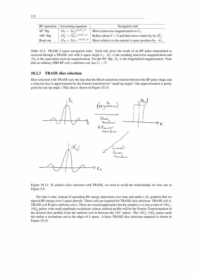
113
RF operation Governing equation Navigation rule90◦ flip MT = Mze
2πi~kJ ·~p Move transverse magnetization to ~kJ .180◦ flip M+
T = M−T e4πi~kJ ·~p Reflect about ~k = ~0 and then move relatively by 2~kJ .
Read out MR = MT e−2πi~kJ ·~p Move relative to the current k-space position by −~kJ .
Table 10.2: TRASE k-space navigation rules. Each rule gives the result of an RF pulse transmitted orreceived through a TRASE coil with k-space origin kJ . MT is the resulting transverse magnetization andMR is the equivalent read out magnetization. For the 90◦ flip, Mz is the longitudinal magnetization. Notethat an ordinary MRI RF coil, a uniform coil, has ~kJ = ~0.
10.2.3 TRASE slice selectionSlice selection with TRASE uses the idea that the Bloch transform relation between the RF pulse shape anda selected slice is approximated by the Fourier transform for “small tip angles” (the approximation is prettygood for any tip angle.) This idea is shown in Figure 10.13.
Figure 10.13: To achieve slice selection with TRASE, we need to recall the relationships we first saw inFigure 5.9.
The idea is that, instead of spreading RF energy deposition over time and under a B0 gradient that wedeposit RF energy over k-space directly. Three coils are required for TRASE slice selection: TRASE coil A,TRASE coil B and a uniform coil u. There are several approaches but the simplest is to run a train of 180◦A–180◦B pulses with small amplitude excitations (whose ordered profile will be the Fourier Transformation ofthe desired slice profile) from the uniform coil in between the 180◦ pulses. The 180◦A–180◦B pulses pushthe earlier u excitations out to the edges of k-space. A basic TRASE slice selection sequence is shown inFigure 10.14.

A Course in MRI 114
Figure 10.14: To achieve slice selection with TRASE, excitations from the uniform coil u are pushed out ink-space with 180◦A–180◦B TRASE RF pulse pairs.

Chapter 11
Image Post Processing: Maps
11.1 Diffusion MapsA diffusion-weighted MR image contains T2 and Da information as given by
Pρ(~p) = KMT (~p) e−TE/T2(~p) e−bDa(~p) (11.1)
where K is an (unknown) constant of proportionality and MT (~p), the transverse magnetization at point ~p,also contains T1(~p) information due to the effect of TR in the imaging sequence.
In many studies we desire to know the distribution of water self-diffusion coefficient as given byDa(~p).One way of obtaining Da(~p) is to do two measurements with the same sequence, one with the diffu-sion gradients turned off (b = 0) and one with them on (b 6= 0). By using the same sequence, the termKMT (~p) e−TE/T2(~p) will be the same for both measurements. Specifically, the unweighted sequence (se-quence 1) produces the image
Pρ1(~p) = KMT (~p) e−TE/T2(~p)
and the weighted sequence (sequence 2) produces
Pρ1(~p) = KMT (~p) e−TE/T2(~p) e−bDa(~p).
Taking the ratio of these two images gives
Pρ2(~p)
Pρ1(~p)= e−bDa(~p)
so
ln
(Pρ2(~p)
Pρ1(~p)
)= −bDa(~p)
Da(~p) = −1
bln
(Pρ2(~p)
Pρ1(~p)
).
The function Da is the diffusion map. Specifically, if ~pmn represents the coordinates of the center ofpixel mn, 1 ≤ m ≤M , 1 ≤ n ≤ N in an N ×M image, then each pixel in the map is computed from
Da(~pmn) =1
bln
(Pρ1(~pmn)
Pρ2(~pmn)
)or, simplifying the notation:
Da(m,n) =1
bln
(Pρ1(m,n)
Pρ2(m,n)
). (11.2)
115

A Course in MRI 116
n = 1 n = 2 n = 1 n = 2
m = 1
m = 2
m = 1
m = 2
100 150
200 170
91 97
148 139
Pρ1 (unweighted) Pρ2 (weighted)
Figure 11.1: Pixel values in example unweighted and weighted diffusion four pixel images.
Example. Suppose we obtain two 2× 2 MR images, one unweighted and one weighted as illustrated inFigure 11.1.where the numbers represent the greyscale values. Typically greyscale values will be 12-bit, that is they willbe between 0 and 4095 = 212 − 1. Zero is black, 4095 is white if the image is not windowed. Windowing,though, only affects the display of the image, the data in the computer are not affected. (Windowing is dis-cussed in Section 11.2.) Calculating the diffusion coefficients pixel by pixel, supposing b = 20, 000s/cm2,gives:
Da(1, 1) =1
20, 000ln
(100
91
)= 47× 10−7cm2/s
Da(1, 2) =1
20, 000ln
(150
97
)= 218× 10−7cm2/s
Da(2, 1) =1
20, 000ln
(200
148
)= 151× 10−7cm2/s
Da(2, 2) =1
20, 000ln
(170
139
)= 101× 10−7cm2/s
resulting in the diffusion map shown in Figure 11.2.
47 218
151 101
Da(×10−7cm2/s)
Figure 11.2: The diffusion map resulting from the data given in Figure 11.1.
Mathematically speaking, two measurements, an unweighted and a weighted, are all that are requiredto produce a diffusion coefficient map. In practice, noise in the images will affect the accuracy of themaps. In fact, noise can sometimes produce a greyscale value in the weighted image that is higher than theunweighted image. When this happens, no Da can be computed for that pixel. (In my research computerprogram, I put Da = 0 when that happens so that any subsequent analysis of the image needs to take intoaccount that Da = 0 means no data are available about Da at that point.) By using more measurementswith different b, and using a least square curve fit, as illustrated in Figure 11.3, a more accurate map can becomputed.

117
Least squares curve for Me−bDaM
Pρ
0 b1 b2 b3 b4
b
data
Figure 11.3: Better diffusion maps can be computed from a series of images with different values of diffu-sion weighting.
11.2 Windowing
Maps can be displayed as images by mapping the range, or a subrange, of the map values into the greyscalerange that can be shown on a computer.
A typical computer display can show 8 bit greyscale (black and white) images. That is, greyscale willvary from 0 to 255 = 28 − 1 and 0 will be black, 255 white and 254 shades of grey will be in between.
Suppose that the maximum diffusion map value was M , then multiplying all the map values by 255/Mwill make the largest Da appear white in the image.
Example. The map of the example in Section 11.1 becomes an image via the scaling shown in Figure11.4 where the maximum map value of 218 was set equal to M .
27 218
151 101
× 255218 =
55 255
177 118
Figure 11.4: Windowing the map of Figure 11.3 so that the maximum value is set to white = 255.
In general, windowing can map or transform the values of a map to arbitrary greyscale values. But themost useful transformation is a linear transformation. The parameters that characterize the linear transform1
are window center, or level, (denoted on Siemens MRI by C) and window width (denoted by W ). Theparameters W and C can typically be adjusted by a couple of dials or via a mouse2. Graphically W and Cspecify the linear transform as follows:
Note that linear windowing with W and C can be, and is, applied to any image, not just maps. So maxis 4095 for standard 12 bit MR images and 0 ≤W,C ≤ 4095.
In the example above, the process of multiplying by 255/M corresponds to W = M , C = M/2.The explicit linear transformation is given by y = ax + b where x is the original image data, y is the
windowed image data and
255 = a
(C +
W
2
)+ b
1Strictly speaking, the transformation is only linear within the window width.2Windowing is typically done automatically for first presentation.
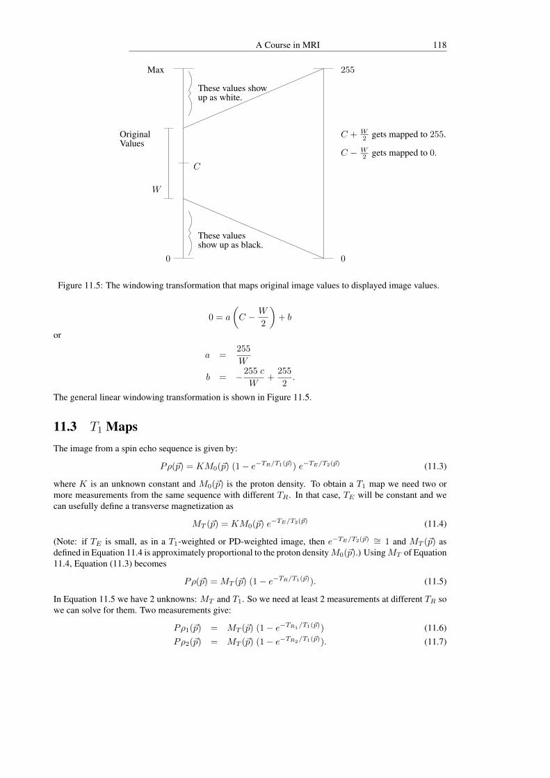
A Course in MRI 118
Max
OriginalValues
W
0
These values showup as white.
These valuesshow up as black.
255
0
C
C + W2 gets mapped to 255.
C − W2 gets mapped to 0.
Figure 11.5: The windowing transformation that maps original image values to displayed image values.
0 = a
(C − W
2
)+ b
or
a =255
W
b = −255 c
W+
255
2.
The general linear windowing transformation is shown in Figure 11.5.
11.3 T1 MapsThe image from a spin echo sequence is given by:
Pρ(~p) = KM0(~p) (1− e−TR/T1(~p)) e−TE/T2(~p) (11.3)
where K is an unknown constant and M0(~p) is the proton density. To obtain a T1 map we need two ormore measurements from the same sequence with different TR. In that case, TE will be constant and wecan usefully define a transverse magnetization as
MT (~p) = KM0(~p) e−TE/T2(~p) (11.4)
(Note: if TE is small, as in a T1-weighted or PD-weighted image, then e−TE/T2(~p) ∼= 1 and MT (~p) asdefined in Equation 11.4 is approximately proportional to the proton densityM0(~p).) UsingMT of Equation11.4, Equation (11.3) becomes
Pρ(~p) = MT (~p) (1− e−TR/T1(~p)). (11.5)
In Equation 11.5 we have 2 unknowns: MT and T1. So we need at least 2 measurements at different TR sowe can solve for them. Two measurements give:
Pρ1(~p) = MT (~p) (1− e−TR1/T1(~p)) (11.6)
Pρ2(~p) = MT (~p) (1− e−TR2/T1(~p)). (11.7)

119
Solving for MT in Equation (11.6) gives
MT (~p) =Pρ1(~p)
(1− e−TR1/T1(~p))
(11.8)
Substituting Equation (11.8) into Equation (11.7) gives
Pρ2(~p) =Pρ1(~p)
(1− e−TR1/T1(~p))
(1− e−TR2/T1(~p))
orPρ2(~p)
Pρ1(~p)=
(1− e−TR2/T1(~p))
(1− e−TR1/T1(~p))
. (11.9)
There is no closed form solution for T1(~p) from Equation (11.9) and T1(~p) must be solved for from Equation(11.9) via a numerical technique like bisection or Newton’s method.
As with the diffusion maps, noise can cause a problem when only two images are used to compute aT1 map. Better maps can be obtained with a least squares fit to data from more than one TR as shownschematically in Figure 11.6.
Pρ
MT ∝M0
MT (1− e−TR/T1)
TR1TR2
TR3TR4
TR
Figure 11.6: Better T1 maps can be made from more than two images.
11.4 T2 MapsIf we usefully define another transverse magnetization quantity,
MT (~p) = KM0(~p) (1− e−TR/T1(~p)),
then Equation (11.3) becomesPρ(~p) = MT (~p) e−TE/T2(~p). (11.10)
To obtain a T2 map we need at least two measurements from the same sequence with different TE . InEquation (11.10) there are two unknowns, MT and T2. MT will be a mixture of T1 and PD weighting so itis of no quantitative use. Two measurements give:
Pρ1(~p) = MT (~p) e−TE1/T2(~p) (11.11)
Pρ2(~p) = MT (~p) e−TE2/T2(~p). (11.12)
Solving for MT in Equation (11.11) gives
MT (~p) =Pρ1(~p)
e−TE1/T2(~p)
. (11.13)
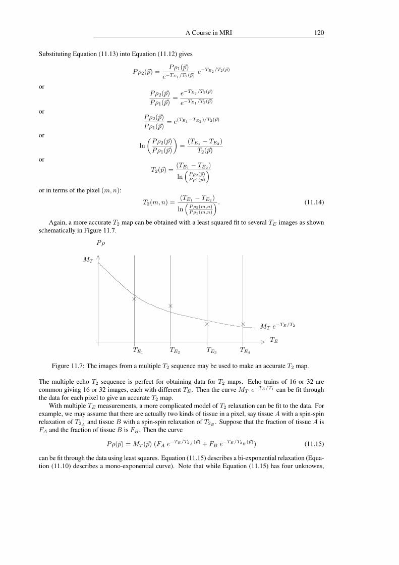
A Course in MRI 120
Substituting Equation (11.13) into Equation (11.12) gives
Pρ2(~p) =Pρ1(~p)
e−TE1/T2(~p)
e−TE2/T2(~p)
orPρ2(~p)
Pρ1(~p)=e−TE2
/T2(~p)
e−TE1/T2(~p)
orPρ2(~p)
Pρ1(~p)= e(TE1
−TE2)/T2(~p)
or
ln
(Pρ2(~p)
Pρ1(~p)
)=
(TE1− TE2
)
T2(~p)
or
T2(~p) =(TE1
− TE2)
ln(Pρ2(~p)Pρ1(~p)
)or in terms of the pixel (m,n):
T2(m,n) =(TE1 − TE2)
ln(Pρ2(m,n)Pρ1(m,n)
) . (11.14)
Again, a more accurate T2 map can be obtained with a least squared fit to several TE images as shownschematically in Figure 11.7.
MT
Pρ
MT e−TE/T2
TE1 TE2 TE3 TE4
TE
Figure 11.7: The images from a multiple T2 sequence may be used to make an accurate T2 map.
The multiple echo T2 sequence is perfect for obtaining data for T2 maps. Echo trains of 16 or 32 arecommon giving 16 or 32 images, each with different TE . Then the curve MT e−TE/T1 can be fit throughthe data for each pixel to give an accurate T2 map.
With multiple TE measurements, a more complicated model of T2 relaxation can be fit to the data. Forexample, we may assume that there are actually two kinds of tissue in a pixel, say tissue A with a spin-spinrelaxation of T2A and tissue B with a spin-spin relaxation of T2B . Suppose that the fraction of tissue A isFA and the fraction of tissue B is FB . Then the curve
Pρ(~p) = MT (~p) (FA e−TE/T2A
(~p) + FB e−TE/T2B(~p)) (11.15)
can be fit through the data using least squares. Equation (11.15) describes a bi-exponential relaxation (Equa-tion (11.10) describes a mono-exponential curve). Note that while Equation (11.15) has four unknowns,

121
T2A , T2B , FA and FB , a minimum of only three measurements are required because FB = (1−FA). Morecomplicated models with more tissue types per pixel are also possible.
Similarly, diffusion models that are more complicated that that of Equation (11.1) can be fit to measure-ments made with multiple b values.
Exercises1. Suppose b = 20, 000 s/cm2 and the two unweighted and weighted diffusion images shown in Figure
11.8 are obtained.
150 150
150 150
112 120
97 130
Pρ1 (unweighted) Pρ2 (weighted)
Figure 11.8: Data for question 1.
Compute the diffusion map using Equation (11.2).
Answer: Shown in Figure 11.9.
146 112
218 72
Da(×10−7 cm2/s)
Figure 11.9: The answer to question 1.
2. Scale (window) the map of the previous exercise to an image where the largest Da is displayed aswhite (255 greyscale).
3. Suppose you have two 2× 2 T2-weighted images with TE as shown in Figure 11.10.
115 120
200 50
TE = 15
70 94
144 41
TE = 40
Figure 11.10: Data for question 3.
Compute the T2 map using Equation (11.14).

A Course in MRI 122
Answer: Shown in Figure 11.11.
50 102
76 126
Figure 11.11: Answer for question 3.

Chapter 12
Diffusion Tensor Imaging
The phenomenon of diffusion usually refers to mass transfer under a concentration gradient as given byFick’s Law:
∂C
∂t= D
(∂2C
∂x2+∂2C
∂y2+∂2C
∂z2
)where C is the concentration and D is the diffusion coefficient. In the case of self-diffusion we are talkingabout Brownian motion. In that case, if the Brownian motion is isotropic, the governing equation is
∂P
∂t= D
(∂2P
∂x2+∂2P
∂y2+∂2P
∂z2
)where P (~q, t) is the probability that a molecule (water) travels a distance ~q in time t.
When the medium is non-isotropic the situation is more complex and cannot be described by a singlediffusion coefficient. In that case correlations, Dab, between velocities can describe the motion:
Dab =
∫ ∞0
〈va(0)vb(t)〉 dt (12.1)
where the 〈〉 denotes average value and a, b are each one of x, y or z. In Brownian motion1, the particlepath looks like that shown in Figure 12.1.
~v(t) = (vx(t), vy(t), vz(t))
Figure 12.1: The path of a particle in Brownian motion. The velocity of the particle is tangent to the pathas shown.
1An ideal Brownian motion path is an example of a curve that is continuous but nowhere differentiable – for all you fans ofnon-intuitive mathematical objects.
123

A Course in MRI 124
The velocity correlations, or diffusion coefficients, of Equation (12.1) lead to a matrix called the diffu-sion tensor:
D =
Dxx Dxy Dxz
Dyx Dyy Dyz
Dzx Dzy Dzz
.Mathematically, D is a second rank tensor. From an abstract point of view, D maps a pair of vectors
(e.g. ~v and ~w in R3 × R3) to a number in R. Explicitly, ~vTD~w is known as a bilinear form2 or generalizedinner product. It generalizes the inner product 〈~v, ~w〉, in fact 〈~v, ~w〉 = ~vT I~w where I is the identity matrix
I =
1 0 00 1 00 0 1
.When ~v = ~w, we have a bilinear form and a distance measure on R3 given by d = ~vTD~v. Again, if D = Iwe have oridinary Euclidian distance on R3: the set of all points at a distance d from the origin is the surfaceof a sphere. When d = ~vTD~v, the set of all points at a distance of d from the origin forms the surface ofan ellipse. This is why D gives such a good description of anisotropic3 diffusion. The surface of an ellipserepresents how far a water molecule can travel in a given interval of time.
12.1 Diffusion Tensor WeightingIf we apply a bipolar gradient in any direction (not just z like before) then it can be shown that the transversemagnetization or image pixel value will be
Pρ(~p) = KMT (~p) e−TE/T2(~p) e−γ2δ2(∆−δ/3)~GTD~G (12.2)
where δ and ∆ are as given in Figure 9.12 and
~GTD~G = [GxGyGz]
Dxx Dxy Dxz
Dyx Dyy Dyz
Dzx Dzy Dzz
GxGyGz
= [GxGyGz]
DxxGx +DxyGy +DxzGzDyzGx +DyyGy +DyzDz
DzxGx +DzyGy +DzzGz
= DxxGxGx +DxyGxGy +DxzGxGz +DyxGyGx +DyyGyGy +DyzGyGz
+ DzxGzGx +DzyGzGy +DzzGzGz.
The diffusion matrix is symmetric. That is Dxy = Dyx, Dxz = Dzx and Dyz = Dzy . So there are only6 distinct diffusion coefficients in the diffusion tensor. To determine these 6 values, and to make a map foreach value, we need a minimum of 7 measurements, one unweighted and 6 weighted with the weightinggradient vector ~G different (non-colinear) in each case. The 6 weighted/unweighted ratios provide sixequations with which to solve for the 6 diffusion coefficients. Of course, more than 6 weighted images withdifferent ~G can be used with least squares methods to get more accurate maps.
It takes a lot of time to obtain 7 MR images. However, many times all that is required is some basicanisotropy information. Before we can talk about anisotropy, recall the basic fact from linear algebra thatyou can always find a rotational transformation R from the original coordinate system (x, y, z) to anothercoordinate system (x′, y′, z′) where a symmetric matrix becomes diagonal. For our diffusion tensor wehave
DD = RTDR2Higher rank tensors are multilinear forms.3Isotropic means “the same in all directions”, anisotropic means “not he same in all directions”.
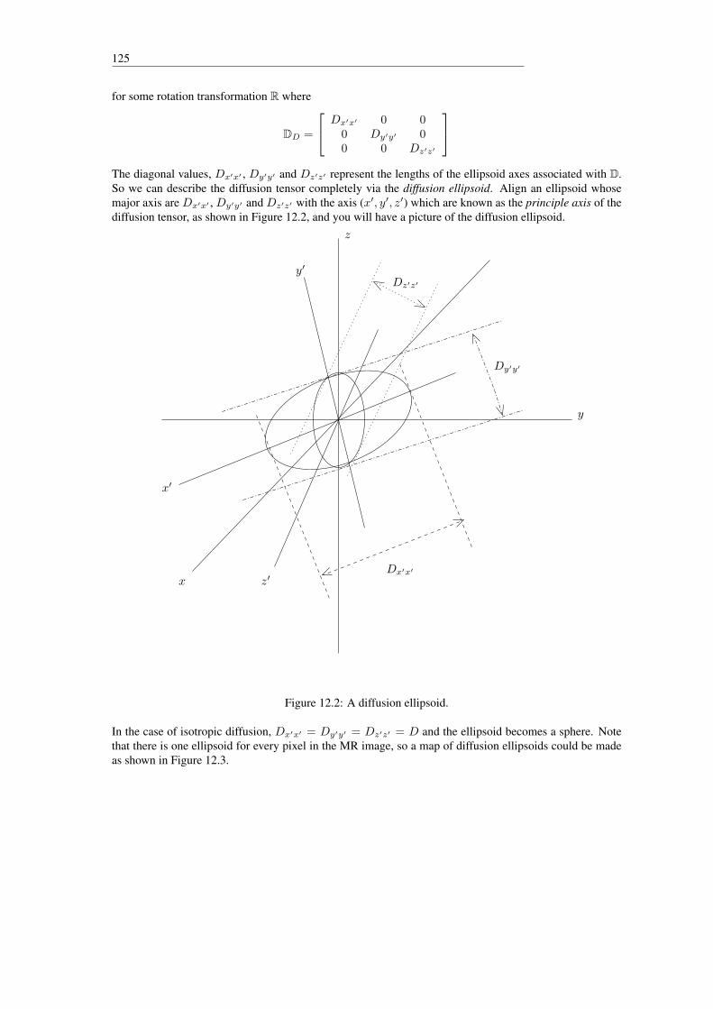
125
for some rotation transformation R where
DD =
Dx′x′ 0 00 Dy′y′ 00 0 Dz′z′
The diagonal values, Dx′x′ , Dy′y′ and Dz′z′ represent the lengths of the ellipsoid axes associated with D.So we can describe the diffusion tensor completely via the diffusion ellipsoid. Align an ellipsoid whosemajor axis are Dx′x′ , Dy′y′ and Dz′z′ with the axis (x′, y′, z′) which are known as the principle axis of thediffusion tensor, as shown in Figure 12.2, and you will have a picture of the diffusion ellipsoid.
������������������������������
������������������������������
������������������������������������������������������������
������������������������������������������������������������������������������������������������������������������������������������������������������������������������������������������������������������������������������������������������������������������������������������������������������������������������������������������������������������������������������������������������������������������������������������������������������������������������������������������������������������������������������������������������������������������������
������������������������������������������������������������������������������������������������������������������������������������������������������������������������������������������������������������������������������������������������������������������������������������������������������������������������������������������������������������������������������������������������������������������������������������������������������������������������������������������������������������������������������������������������������������������������
������������������������������������������������������������������������������������������������������������������������������������������������
������������������������������������������������������������������������������������������������������������������������������������������������
������������������������������������������������������������������������������������������������������������������������������������������������������������������������������������������������������������������
������������������������������������������������������������������������������������������������������������������������������������������������������������������������������������������������������������������
x
y
z
z′
x′
y′
Dz′z′
Dy′y′
Dx′x′
Figure 12.2: A diffusion ellipsoid.
In the case of isotropic diffusion, Dx′x′ = Dy′y′ = Dz′z′ = D and the ellipsoid becomes a sphere. Notethat there is one ellipsoid for every pixel in the MR image, so a map of diffusion ellipsoids could be madeas shown in Figure 12.3.

A Course in MRI 126
Figure 12.3: An example diffusion tensor map. Note the little cylinders that represent the diffusion ellip-soids. This illustration was taken from some Siemens promotional literature.
As mentioned earlier, the diffusion ellipsoid can be thought of as the surface that a water molecule willmost likely end up on if it were placed at the center of the ellipsoid and allowed to diffuse for a fixed amountof time. So, in general, if each dot in Figure 12.4 represents where the water molecule actually is after afixed time period, the result of several such “thought experiments” will be as shown in Figure 12.4.
Figure 12.4: The dots represent the posible positions of a water molecule that started out at the origin andwas allowed to diffuse for a fixed period of time. Note that the diffusion ellipsoid represents the averagelocation of a whole bunch of water molecules after they have been allowed to diffuse for a fixed time periodfrom the origin. This illustration was ripped off from some unidentified web site.
A long diffusion ellipsoid like that shown in Figure 12.4 will result if there is more restriction to waterdiffusion in one direction than in another. For example, in a neuron there is relatively little restriction towater diffusion along the axon, but there is no easy way for the water to get out of the cell perpendicular tothe axon.
In the case that there are no restrictions to diffusion, the diffusion ellipsoid becomes a sphere and theresults of our “thought experiment” will look like Figure 12.5.
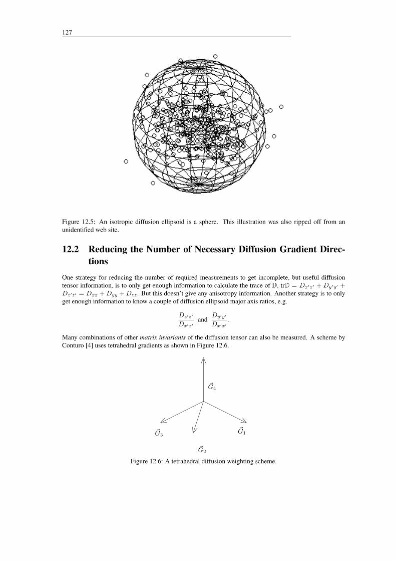
127
Figure 12.5: An isotropic diffusion ellipsoid is a sphere. This illustration was also ripped off from anunidentified web site.
12.2 Reducing the Number of Necessary Diffusion Gradient Direc-tions
One strategy for reducing the number of required measurements to get incomplete, but useful diffusiontensor information, is to only get enough information to calculate the trace of D, trD = Dx′x′ + Dy′y′ +Dz′z′ = Dxx +Dyy +Dzz . But this doesn’t give any anisotropy information. Another strategy is to onlyget enough information to know a couple of diffusion ellipsoid major axis ratios, e.g.
Dz′z′
Dx′x′and
Dy′y′
Dx′x′.
Many combinations of other matrix invariants of the diffusion tensor can also be measured. A scheme byConturo [4] uses tetrahedral gradients as shown in Figure 12.6.
~G1
~G2
~G3
~G4
Figure 12.6: A tetrahedral diffusion weighting scheme.

A Course in MRI 128
The use of tetrahedral gradients reduces the total number of measurements from 7 to 5 and gives trD,D‖ and D⊥ where D‖ and D⊥ represent apparent diffusion coefficients that would be obtained if thediffusion gradients were aligned parallel and perpendicular to the diffusion ellipsoid’s axes. The assumptionto make the computation of D⊥ possible is that the diffusion ellipsoid exhibits cylindrical symmetry. Thatis, Dy′y′ = Dz′z′ for the smaller axes.
12.3 Elements and Measures of Diffusion AnisotropyTo recap, a water molecule diffusing in water will follow a random walk path due to Brownian motionand if we look at the end point of all the random walks that start at the origin we will get a diffusionellipsoid. The diffusion ellipsoid may be thought of as representing the one standard deviation surface of amultivariate normal distribution whose axis lengths are given by σx′ =
√2Dx′x′∆, σy′ =
√2Dy′y′∆ and
σz′ =√
2Dz′z′∆ where ∆ is the time between bipolar gradient pulses (see Figure 9.12).If the direction of the bipolar gradient is ~G then, rewriting Equation (12.2) using the difinition of b from
Equation (9.4) or (9.3) gives a diffusion weighted image
Pρ(~p) = KMT (~p)e−TET2(~p) e−b
~GTD~G.
With 6 gradient directions we obtain 6 images Pρ1 , Pρ2 , ... , Pρ6 , each with different diffusion weighting.If we also obtain an unweighted image Pρ0 then we can compute 6 ratio (attenuation) images
Pρ1Pρ0
,Pρ2Pρ0
, . . . ,Pρ6Pρ0
.
From these ratios, 6 diffusion coefficient images can be computed, by taking the natural log of each ratioand dividing by b, and subsequently the D matrix can be computed for each pixel. The D matrix for eachpixel can be transformed to the principle direction by a suitable rotation D = RTDR giving a diagonalmatrix
DD =
Dx′x′ 0 00 Dy′y′ 00 0 Dz′z′
=
λx 0 00 λy 00 0 λz
for each pixel.
From the diffusion matrix we can compute the widely used fractional anisotropy, FA, using
FA =
√3√
(λx − λ)2 + (λy − λ)2 + (λz − λ)2
√2√λ2x + λ2
y + λ2z
(12.3)
whereλ =
1
3(λx + λy + λz) =
1
3(Dxx +Dyy +Dzz)
is the 13 the trace of the diffusion tensor. The trace of the diffusion tensor is another widely used measure
and is given byTr(D) = λx + λy + λz = Dxx +Dyy +Dzz. (12.4)
Note that trace is invariant under rotation transformations – a basic fact from linear algebra. We can alsocompute two elements of anisotropy:
η =1
3(λx −
λy + λz2
) (12.5)
which measures how long the ellipsoid is and
ε =λy − λz
2(12.6)

129
which measures how round the ellipsoid is. In Equations (12.5) and (12.6) we have assumed that λx >λy > λz . If ε = 0 then we say that the diffusion ellipsoid is cylindrically symmetrical. In that case λy = λzand we’d only need 5 measurements instead of 7 to get diffusion tensor data as discussed in Section 12.2.Neural tissue generally produces cylindrically symmetrical diffusion tensors.
By plotting an oriented line matched to the direction of the major axis of the diffusion ellipsoid, we canfollow fibre tracts in the brain.
A single diffusion weighted image (along with an unweighted image) will give rise to the map:
D = −1
bln
(PρweightedPρunweighted
)
The value of D will vary with the direction of ~G. A plot of the magnitude of D with direction gives, in
general, a peanut-shaped surface as shown in Figure 12.7 where D =
4 0 00 1 00 0 1
.
-4-3
-2-1
0 1
2 3
4-2-1.5
-1-0.5
0 0.5
1 1.5
2
-2
-1.5
-1
-0.5
0
0.5
1
1.5
2
z
xy
z-4
-3-2
-1 0
1 2
3 4-1-0.8-0.6-0.4-0.2 0
0.2 0.4 0.6 0.8 1
-1
-0.5
0
0.5
1
z
x
y
z
Figure 12.7: A plot of D is shown on the left that results from the diffusion tensor D described in the text.The associated diffusion ellipsoid is shown on the right.
The surface shown in Figure 12.7, left, is called by some the diffusion tensor. But that is not mathemat-ically correct language. The bilinear map that the diffusion matrix represents is the mathematical diffusiontensor. The ”D-surface” of Figure 12.7 is explicitly the surface ~s = (~vTD~v)~v where ~v ∈ S2, the unit sphere.The diffusion ellipsoid is ~s = D~v. The vector ~v represents the direction of ~G.
There may be more than one diffusion ellipsoid in a given voxel. In that case many measurements (morethan six ~G directions) at varying b levels are required to measure several D-surfaces (they change with b)and ultimately to solve for the underlying diffusion ellipsoids in the voxel. This approach is necessary toresolve crossed white matter fibres in the brain.
12.4 Other Diffusion MethodsOther approaches to diffusion imaging include the following.
• Multi-compontent models – a simplification of multi diffusion ellipsoid models that assume isotropicdiffusion. For example, a two compartment model give the following image [14]:
Pρ(~ρ) = KMT (~ρ)(νae−bDa + νbe
−bDb) (12.7)
In addition to unweighted Pρ0, four weighted measurements would be required (all at different b) tosolve for νa, νb, Da and Db in the isotropic two compartment model.
• q-space. This method is essentially Fourier transformation with respect to b to reveal a spectrum ofD values. Many measurements at multiple b are required.

A Course in MRI 130
• Single-shot ADC. A method that uses EPI to acquire one unweighted and two weighted (two valuesof b) in short TE has been reported by Song et al. [22]. The single-shot ADC acquisition can berepeated at a set TR and give functional brain maps with a contrast based on functionally relatedADC changes instead of the usual BOLD changes (see Chapter 14) which are suppressed by usingshort TE .
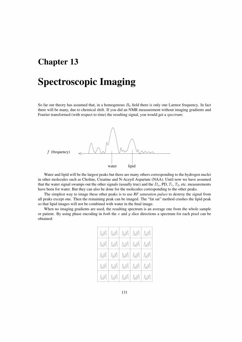
Chapter 13
Spectroscopic Imaging
So far our theory has assumed that, in a homogenous B0 field there is only one Larmor frequency. In factthere will be many, due to chemical shift. If you did an NMR measurement without imaging gradients andFourier transformed (with respect to time) the resulting signal, you would get a spectrum:
water lipid
f (frequency)
Water and lipid will be the largest peaks but there are many others corresponding to the hydrogen nucleiin other molecules such as Choline, Creatine and N-Aceytl Aspartate (NAA). Until now we have assumedthat the water signal swamps out the other signals (usually true) and the Da, PD, T1, T2, etc. measurementshave been for water. But they can also be done for the molecules corresponding to the other peaks.
The simplest way to image these other peaks is to use RF saturation pulses to destroy the signal fromall peaks except one. Then the remaining peak can be imaged. The “fat sat” method crushes the lipid peakso that lipid images will not be combined with water in the final image.
When no imaging gradients are used, the resulting spectrum is an average one from the whole sampleor patient. By using phase encoding in both the x and y slice directions a spectrum for each pixel can beobtained:
131
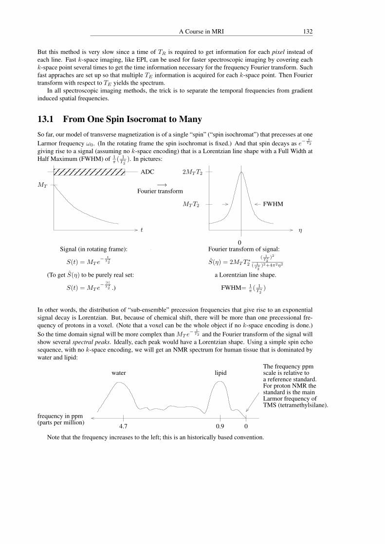
A Course in MRI 132
But this method is very slow since a time of TR is required to get information for each pixel instead ofeach line. Fast k-space imaging, like EPI, can be used for faster spectroscopic imaging by covering eachk-space point several times to get the time information necessary for the frequency Fourier transform. Suchfast appraches are set up so that multiple TE information is acquired for each k-space point. Then Fouriertransform with respect to TE yields the spectrum.
In all spectroscopic imaging methods, the trick is to separate the temporal frequencies from gradientinduced spatial frequencies.
13.1 From One Spin Isocromat to ManySo far, our model of transverse magnetization is of a single “spin” (“spin isochromat”) that precesses at oneLarmor frequency ω0. (In the rotating frame the spin isochromat is fixed.) And that spin decays as e−
tT2
giving rise to a signal (assuming no k-space encoding) that is a Lorentzian line shape with a Full Width atHalf Maximum (FWHM) of 1
π ( 1T∗2
). In pictures:
MT
ADC
t
−→Fourier transform
2MTT2
MTT2 FWHM
0
η
Signal (in rotating frame):
S(t) = MT e− tT∗2
(To get S(η) to be purely real set:
S(t) = MT e− |t|T∗2 .)
Fourier transform of signal:
S(η) = 2MTT∗2
( 1T∗2
)2
( 1T∗2
)2+4π2η2
a Lorentzian line shape.
FWHM= 1π ( 1
T∗2)
In other words, the distribution of “sub-ensemble” precession frequencies that give rise to an exponentialsignal decay is Lorentzian. But, because of chemical shift, there will be more than one precessional fre-quency of protons in a voxel. (Note that a voxel can be the whole object if no k-space encoding is done.)So the time domain signal will be more complex than MT e
− tT2 and the Fourier transform of the signal will
show several spectral peaks. Ideally, each peak would have a Lorentzian shape. Using a simple spin echosequence, with no k-space encoding, we will get an NMR spectrum for human tissue that is dominated bywater and lipid:
4.7 0.9 0
frequency in ppm(parts per million)
water lipidThe frequency ppmscale is relative toa reference standard.For proton NMR thestandard is the mainLarmor frequency ofTMS (tetramethylsilane).
Note that the frequency increases to the left; this is an historically based convention.
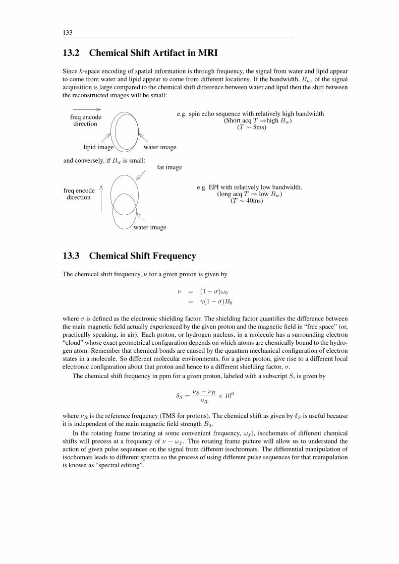
133
13.2 Chemical Shift Artifact in MRI
Since k-space encoding of spatial information is through frequency, the signal from water and lipid appearto come from water and lipid appear to come from different locations. If the bandwidth, Bw, of the signalacquisition is large compared to the chemical shift difference between water and lipid then the shift betweenthe reconstructed images will be small:
freq encodedirection
lipid image water image
and conversely, if Bw is small:
freq encodedirection
fat image
water image
e.g. spin echo sequence with relatively high bandwidth(Short acq T ⇒high Bw)
(T ∼ 5ms)
e.g. EPI with relatively low bandwidth.(long acq T ⇒ low Bw)
(T ∼ 40ms)
13.3 Chemical Shift Frequency
The chemical shift frequency, ν for a given proton is given by
ν = (1− σ)ω0
= γ(1− σ)B0
where σ is defined as the electronic shielding factor. The shielding factor quantifies the difference betweenthe main magnetic field actually experienced by the given proton and the magnetic field in “free space” (or,practically speaking, in air). Each proton, or hydrogen nucleus, in a molecule has a surrounding electron“cloud” whose exact geometrical configuration depends on which atoms are chemically bound to the hydro-gen atom. Remember that chemical bonds are caused by the quantum mechanical configuration of electronstates in a molecule. So different molecular environments, for a given proton, give rise to a different localelectronic configuration about that proton and hence to a different shielding factor, σ.
The chemical shift frequency in ppm for a given proton, labeled with a subscript S, is given by
δS =νS − νRνR
× 106
where νR is the reference frequency (TMS for protons). The chemical shift as given by δS is useful becauseit is independent of the main magnetic field strength B0.
In the rotating frame (rotating at some convenient frequency, ωf ), isochomats of different chemicalshifts will precess at a frequency of ν − ωf . This rotating frame picture will allow us to understand theaction of given pulse sequences on the signal from different isochromats. The differential manipulation ofisochomats leads to different spectra so the process of using different pulse sequences for that manipulationis known as “spectral editing”.

A Course in MRI 134
13.4 J CouplingProton spins in one section of a molecule can interact with proton spins in another section of molecule be-cause the spins, or magnetic moments, generate magnetic fields of their own. The magnetic field associatedwith one spin can affect the precession frequency of a nearby spin and vice versa. The effect of this “Jcoupling” is to split spectral lines:
splits to
The peaks will be separated by J Hz independent of B0, so in a ppm diagram the spacing between peaksdepends on B0 while the position of the peaks does not.
If you pick ωf to be the middle frequency between a pair of coupled lines:
ωf
the isochromats for each line will precess at ±J2 frequency in the rotating frame:z
J2
J2
y
x
13.5 The Really Important Molecules
13.5.1 Water (H2O)The most abundant molecule in the human body is water with the familiar chemical structure:
O
HH
chemically equivalent protons
As indicated in the diagram, the two hydrogen atoms are “chemically equivalent” because the local elec-tronic environment is the same for both atoms. Therefore the chemical shift for each proton will be thesame at 4.7 ppm.
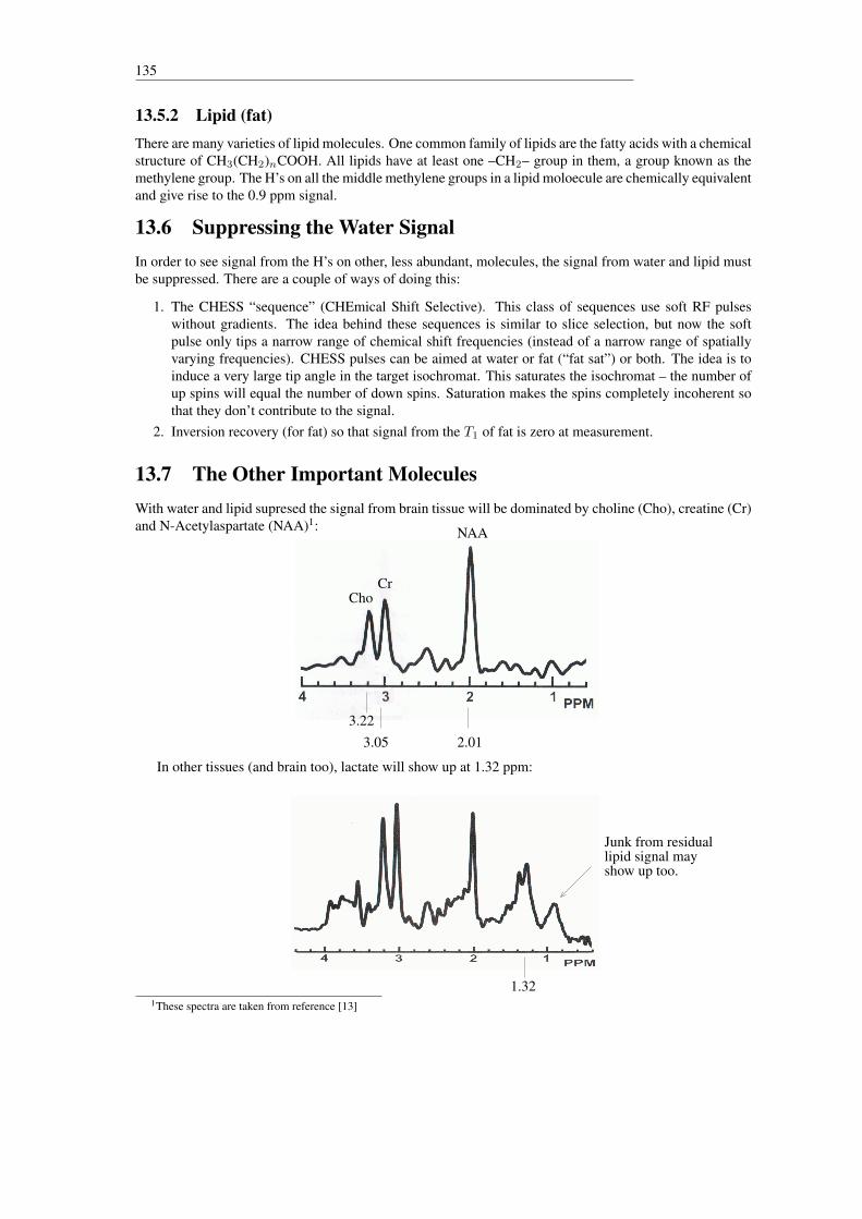
135
13.5.2 Lipid (fat)There are many varieties of lipid molecules. One common family of lipids are the fatty acids with a chemicalstructure of CH3(CH2)nCOOH. All lipids have at least one –CH2– group in them, a group known as themethylene group. The H’s on all the middle methylene groups in a lipid moloecule are chemically equivalentand give rise to the 0.9 ppm signal.
13.6 Suppressing the Water SignalIn order to see signal from the H’s on other, less abundant, molecules, the signal from water and lipid mustbe suppressed. There are a couple of ways of doing this:
1. The CHESS “sequence” (CHEmical Shift Selective). This class of sequences use soft RF pulseswithout gradients. The idea behind these sequences is similar to slice selection, but now the softpulse only tips a narrow range of chemical shift frequencies (instead of a narrow range of spatiallyvarying frequencies). CHESS pulses can be aimed at water or fat (“fat sat”) or both. The idea is toinduce a very large tip angle in the target isochromat. This saturates the isochromat – the number ofup spins will equal the number of down spins. Saturation makes the spins completely incoherent sothat they don’t contribute to the signal.
2. Inversion recovery (for fat) so that signal from the T1 of fat is zero at measurement.
13.7 The Other Important MoleculesWith water and lipid supresed the signal from brain tissue will be dominated by choline (Cho), creatine (Cr)and N-Acetylaspartate (NAA)1:
ChoCr
NAA
3.223.05 2.01
In other tissues (and brain too), lactate will show up at 1.32 ppm:
1.32
lactate Junk from residuallipid signal mayshow up too.
1These spectra are taken from reference [13]

A Course in MRI 136
The signals associated with each spectral peak don’t come from the molecules per se, but from specificH’s in the molecules. Each molecule generally has several chemically inequivalent protons and so will beassociated with several lines in a tissue spectrum.
There are several computer software packages that can compute the all chemical shift frequencies of theprotons in a given molecule based on the chemical structure that each H atom is a part of. Below, for eachmolecule discussed, we give the output of one such computer program: NUTS – NMR Utility TransformSoftware which is available on the World Wide Web at URL http:\\ www.acornnmr.com.
13.7.1 LactateThe predictions for the proton frequencies in lactate given by NUTS are:
Node Shift Base + Inc. Comment (ppm rel. to TMS)CH 4.27 1.50 methine
0.17 1 alpha -C1.73 1 alpha -O0.87 1 alpha -C(=O)O
CH3 1.34 0.86 methyl0.25 1 beta -O0.23 1 beta -C(=O)O
OH 2.0 2.00 alcoholOH 11.0 11.00 carboxylic acid
The second column is labeled “Shift”; this is the chemical shift in ppm relative to TMS. The third columnis labeled “Base + Inc.”, to be read with the “Comment” column, and shows how NUTS arrived at thechemical shift frequency. For example, the protons in the CH3 methyl group would have a base chemicalshift of 0.86 ppm on the basis of the magnetic sheilding provided by an electron cloud around a “freefloating” CH3 group; the base electron cloud is modified by the electron cloud of nearby chemically boundatoms which are, for the methyl group, a nearby “beta” oxygen atom (add 0.25 ppm to the base 0.86 ppm)and a nearby beta carbon atom (the one with two oxygen atoms stuck to it, one via a double bond - addanother 0.23 ppm). Adding 0.86 + 0.25 + 0.23 gives the prediction of 1.34 for lactate’s methyl group’shydrogen nuclei. Detailed information on how to compute NMR chemical shifts may be found in [23](basic) and [25] (more detailed). With those predictions, let’s take a look at the chemical structure of lactateto see where the proton “Nodes” are.
The “skeleton” formula (a chemist’s shorthand) for lactate may be seen in chemistry books written aseither
H C3 CO2ï
OHH C3
O
OHOH
or
Skeleton formulae are missing implied C’s and H’s that every chemist considers obvious (because carbonhas 4 covalent bonds). I find it helpful to fill in the implied C’s and H’s:
OHHH
C C C
OH
H
O H
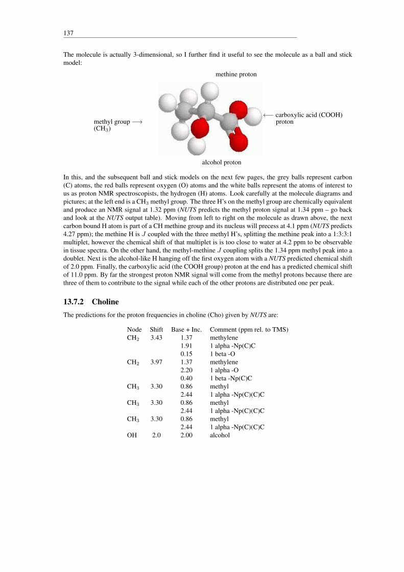
137
The molecule is actually 3-dimensional, so I further find it useful to see the molecule as a ball and stickmodel:
methyl group −→(CH3)
methine proton
←− carboxylic acid (COOH)proton
alcohol proton
In this, and the subsequent ball and stick models on the next few pages, the grey balls represent carbon(C) atoms, the red balls represent oxygen (O) atoms and the white balls represent the atoms of interest tous as proton NMR spectroscopists, the hydrogen (H) atoms. Look carefully at the molecule diagrams andpictures; at the left end is a CH3 methyl group. The three H’s on the methyl group are chemically equivalentand produce an NMR signal at 1.32 ppm (NUTS predicts the methyl proton signal at 1.34 ppm – go backand look at the NUTS output table). Moving from left to right on the molecule as drawn above, the nextcarbon bound H atom is part of a CH methine group and its nucleus will precess at 4.1 ppm (NUTS predicts4.27 ppm); the methine H is J coupled with the three methyl H’s, splitting the methine peak into a 1:3:3:1multiplet, however the chemical shift of that multiplet is is too close to water at 4.2 ppm to be observablein tissue spectra. On the other hand, the methyl-methine J coupling splits the 1.34 ppm methyl peak into adoublet. Next is the alcohol-like H hanging off the first oxygen atom with a NUTS predicted chemical shiftof 2.0 ppm. Finally, the carboxylic acid (the COOH group) proton at the end has a predicted chemical shiftof 11.0 ppm. By far the strongest proton NMR signal will come from the methyl protons because there arethree of them to contribute to the signal while each of the other protons are distributed one per peak.
13.7.2 CholineThe predictions for the proton frequencies in choline (Cho) given by NUTS are:
Node Shift Base + Inc. Comment (ppm rel. to TMS)CH2 3.43 1.37 methylene
1.91 1 alpha -Np(C)C0.15 1 beta -O
CH2 3.97 1.37 methylene2.20 1 alpha -O0.40 1 beta -Np(C)C
CH3 3.30 0.86 methyl2.44 1 alpha -Np(C)(C)C
CH3 3.30 0.86 methyl2.44 1 alpha -Np(C)(C)C
CH3 3.30 0.86 methyl2.44 1 alpha -Np(C)(C)C
OH 2.0 2.00 alcohol
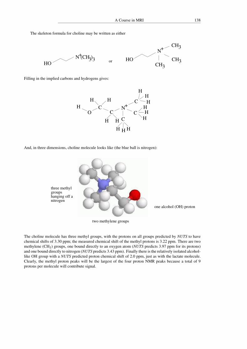
A Course in MRI 138
The skeleton formula for choline may be written as either
N (CH )33+
HO
N+CH3
CH3CH3HOor
Filling in the implied carbons and hydrogens gives:
N+H H
OCH
CC
CHHH HH
HHH
C
HHH
And, in three dimensions, choline molecule looks like (the blue ball is nitrogen):
three methylgroupshanging off anitrogen
two methylene groups
one alcohol (OH) proton
The choline molecule has three methyl groups, with the protons on all groups predicted by NUTS to havechemical shifts of 3.30 ppm; the measured chemical shift of the methyl protons is 3.22 ppm. There are twomethylene (CH2) groups, one bound directly to an oxygen atom (NUTS predicts 3.97 ppm for its protons)and one bound directly to nitrogen (NUTS predicts 3.43 ppm). Finally there is the relatively isolated alcohol-like OH group with a NUTS predicted proton chemical shift of 2.0 ppm, just as with the lactate molecule.Clearly, the methyl proton peaks will be the largest of the four proton NMR peaks because a total of 9protons per molecule will contribute signal.

139
13.7.3 CreatineThe predictions for the proton frequencies in creatine (Cr) given by NUTS are:
Node Shift Base + Inc. Comment (ppm rel. to TMS)CH2 3.49 1.37 methylene
1.22 1 alpha -N-C0.90 1 alpha -C(=O)O
CH3 2.47 0.86 methyl1.61 1 alpha -N
NH2 2.0 2.00 amineNH ? n.a. not estimatedOH 11.0 11.00 carboxylic acid
The skeleton formula for creatine may written as either
H N2N H+ 2
H C3CO2
ï
NHO
ON
NH
NH2
CH3or
Filling in the implied carbons and hydrogens gives:
OH C C N C N HH
N H
C
H HH
H
H
O
And, in three dimensions, creatine molecule looks like:
methyl group
carboxylic acid −→(COOH) proton
methylene group amine group
The creatine molecule has one methyl group and NUTS predicts that its chemically equivalent hydrogenswill have a chemical shift of 2.47 ppm; they show up at 2.47 ppm on the spectrum on page 135. For theremaining protons, NUTS predicts the following frequencies. The methylene protons are at 3.49 ppm, thecarboxylic acid protons are at 11.0 ppm (as with the lactate molecule), the amine proton is at 2.0 ppm andthe chemical shift frequency of the H in the NH group is not estimated.
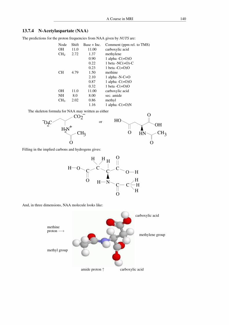
A Course in MRI 140
13.7.4 N-Acetylaspartate (NAA)The predictions for the proton frequencies from NAA given by NUTS are:
Node Shift Base + Inc. Comment (ppm rel. to TMS)OH 11.0 11.00 carboxylic acidCH2 2.72 1.37 methylene
0.90 1 alpha -C(=O)O0.22 1 beta -NC(=O)-C0.23 1 beta -C(=O)O
CH 4.79 1.50 methine2.10 1 alpha -N-C=O0.87 1 alpha -C(=O)O0.32 1 beta -C(=O)O
OH 11.0 11.00 carboxylic acidNH 8.0 8.00 sec. amideCH3 2.02 0.86 methyl
1.16 1 alpha -C(=O)N
The skeleton formula for NAA may written as either
O C2ï
CO2ï
H N2+
CH3O
HO
O
O
OH
HN CH3O
or
Filling in the implied carbons and hydrogens gives:
HHH
H O CC C CO H
HOH H
NO H C C
O
And, in three dimensions, NAA molecule looks like:
methyl group
carboxylic acid
carboxylic acid
methylene group
methineproton −→
amide proton ↑
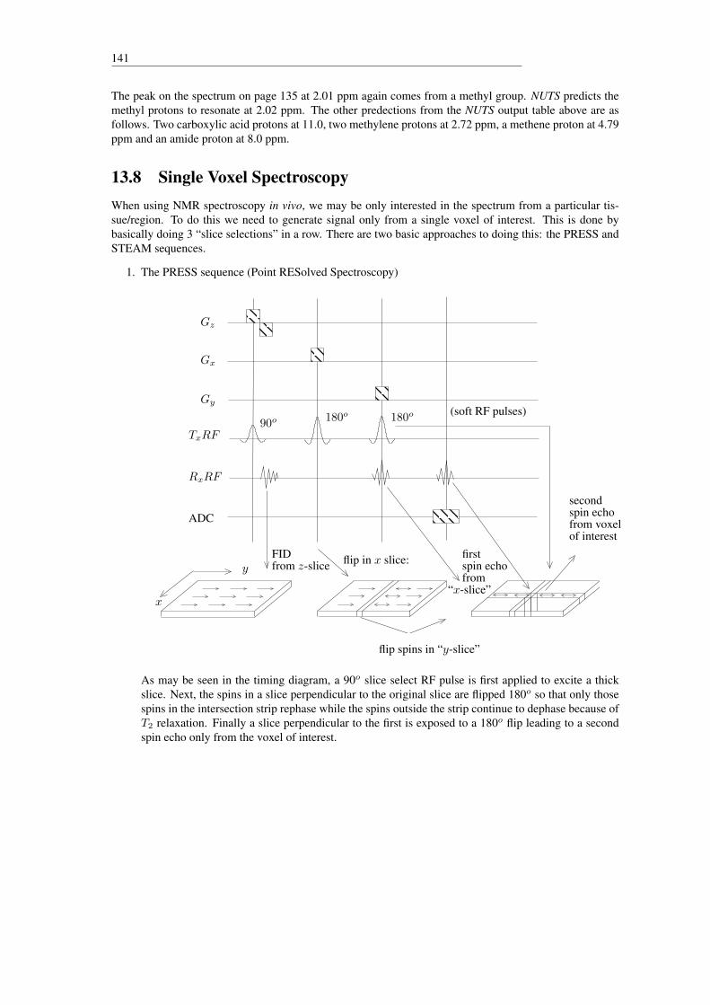
141
The peak on the spectrum on page 135 at 2.01 ppm again comes from a methyl group. NUTS predicts themethyl protons to resonate at 2.02 ppm. The other predections from the NUTS output table above are asfollows. Two carboxylic acid protons at 11.0, two methylene protons at 2.72 ppm, a methene proton at 4.79ppm and an amide proton at 8.0 ppm.
13.8 Single Voxel SpectroscopyWhen using NMR spectroscopy in vivo, we may be only interested in the spectrum from a particular tis-sue/region. To do this we need to generate signal only from a single voxel of interest. This is done bybasically doing 3 “slice selections” in a row. There are two basic approaches to doing this: the PRESS andSTEAM sequences.
1. The PRESS sequence (Point RESolved Spectroscopy)
Gz
Gx
Gy
TxRF
RxRF
ADC
90o 180o 180o (soft RF pulses)
x
yFIDfrom z-slice flip in x slice: first
spin echofrom
“x-slice”
flip spins in “y-slice”
secondspin echofrom voxelof interest
As may be seen in the timing diagram, a 90o slice select RF pulse is first applied to excite a thickslice. Next, the spins in a slice perpendicular to the original slice are flipped 180o so that only thosespins in the intersection strip rephase while the spins outside the strip continue to dephase because ofT2 relaxation. Finally a slice perpendicular to the first is exposed to a 180o flip leading to a secondspin echo only from the voxel of interest.
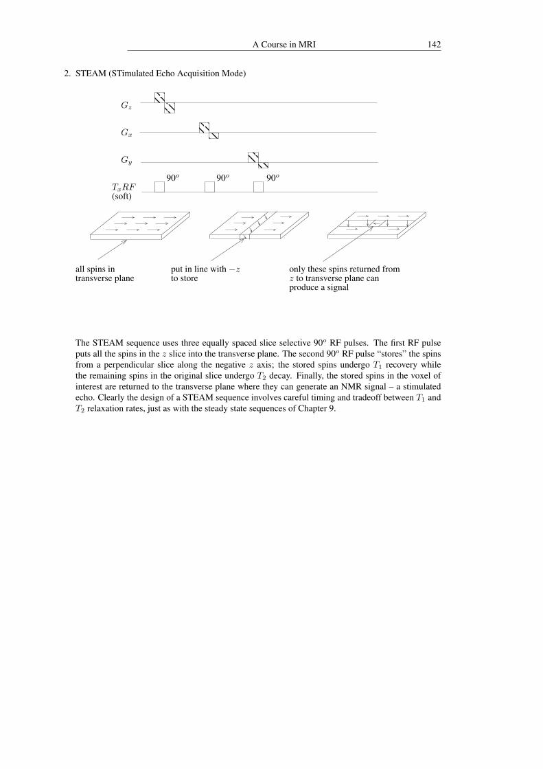
A Course in MRI 142
2. STEAM (STimulated Echo Acquisition Mode)
Gz
Gx
Gy
TxRF(soft)
90o 90o 90o
all spins intransverse plane
put in line with −zto store
only these spins returned fromz to transverse plane canproduce a signal
The STEAM sequence uses three equally spaced slice selective 90o RF pulses. The first RF pulseputs all the spins in the z slice into the transverse plane. The second 90o RF pulse “stores” the spinsfrom a perpendicular slice along the negative z axis; the stored spins undergo T1 recovery whilethe remaining spins in the original slice undergo T2 decay. Finally, the stored spins in the voxel ofinterest are returned to the transverse plane where they can generate an NMR signal – a stimulatedecho. Clearly the design of a STEAM sequence involves careful timing and tradeoff between T1 andT2 relaxation rates, just as with the steady state sequences of Chapter 9.

143
13.9 Spectroscopic ImagingBasic spin echo spectroscopic imaging is accomplished with the a sequence whose timeing diagram lookslike:
Gz
Gx
Gy
TxRF
RxRF
ADC
τi
j
k
90o 180o
water (and/or fat)saturation pulse
TE
Phase encode all k-space info.Acquire signal without gradients.
Acquisitions will be indexed by i, j and k (corresponding to the value of Gx, Gy and Gz phase encodinggradients, respectively); giving signals Sijk(t), one for each 1 ≤ i ≤ I , 1 < j ≤ J and 1 ≤ k ≤ K. Thek-space postition associated with each acquisition is
~ki,j,k =
kx;i,j,k
ky;i,j,k
kz;i,j,k
=γ
2π
Gx;i,j,kτGy;i,j,kτGz;i,j,kτ
Each voxel, centered on ~p, then yields a time domain signal
T (~p, t`) =
K∑k=1
J∑j=1
I∑i=1
Sijk(t`)e−2πi(~p·~ki,j,k
A fourth Fourier Transform gives a spectrum for each voxel:
T (~p, ηm) =
L∑`=1
T (~p, t`)e−2πit`ηm
With phase encoded spectroscopic imaging, each k-space data point requires TR time (minimum –with one signal averaging) to acquire. This is essentially an order of magnitude slower than the singleisochromat imaging techniques we have seen before. Therefore the total number of phase encodes must be

A Course in MRI 144
kept relatively small to reduce acquisition time. An acquisition matrix of 16× 16× 8 (I × J ×K) wouldbe a relatively large acquisition. Also the voxels have to be large because signal coming from each voxel isalot less when the water and fat signals are eliminated.
A faster way to accomplish spectrocsopic imaging is to use EPI. An EPI spectroscopic imaging sequencetiming diagram looks like:
Gz
Gx
Gy
TxRF
RxRF
ADC
90o H20 Sat 180o
frequency
“phase”
slice
(TE)i (variable TE)
This sequence will give a series of EPI images, one for each 1 ≤ i ≤ I , each with slightly different TE .From each pixel (voxel) we get a “time series”, or time domain signal, in which TE is the time:
Intensity
TE
A Fourier transform with respect to TE will give an NMR spectrum for that pixel.

145
13.10 Non-Chemical-Shift Spectroscopic Dimensions
13.10.1 J coupling and the Nuclear Overhauser Effect (nOe)A proton spin may be J coupled to another proton as we’ve seen, causing a line split. A proton (H nucleus)may also be coupled to other species of nuclei like carbon (C). The J coupling effects may be manipulatedby saturating the spin that an H of interest is coupled to. If the coupled spin is another type of nucleus (e.g.C) then RF transmission at that nucleus’s frequency is needed to saturate it. (the gyromagnetic ratios, λ,for different nuclei are different – see the table below.) Saturating one nucleus effectively transfers energyto another, formerly J coupled, nucleus in a process called polarization transfer or magnetization transfer.The phenomenon of polarization transfer may be quantified by using a “compartment model” [10] in whichspin energy may be transferered from a compartment occupied by one nuclear species to a compartmentoccupied by another nuclear species.
For reference, the following table gives the gyromagnetic ratios and quantum spin number I of nucleithat have been used for MRI of the human body.
Nucleus Spin Number γ/2π (MHz/T)1H 1/2 42.6
23Na 3/2 11.331P 1/2 17.2
Of course, with the RF hardware operating at the appropriate frequency, NMR signal from these other (farless abundant than H) nuclear species may be generated. Current clinical MRIs only have RF equipmentcapable of generating radio waves at frequencies in a narrow band around the proton resonance frequencyat the design B0 of the MRI.
When one of the spin sytems in a coupled spin system is saturated, it’s quantum mechanical energylevels are essentially removed from the scene. The effect is to increase the strength of the remaining signalby a factor of η. This increase is the nOe. There are two basic forms of nOe:
• Homonuclear nOe where the saturation nuclear spin species same as signal spin species.
• Heteronuclear nOe where the saturation spin species is different from signal spin species.
The technique of “proton decoupling” or saturating proton spins is almost universally used when obtain-ing NMR spectra from nuclei other than H so that heteronuclear nOe will increase the received NMR signal.The exact mechanism of nOe in each case depends on the number of available T1 “relaxation pathways”.
The basic sequence for polarization transfer is the INEPT (Insensitive Nuclei Enhanced by PolarizationTransfer). An INEPT sequence for 1H and 13C would have the following basic structure:
1H RF frequency: (π2 )x – tD – πx – tD – (π2 )y13C RF frequency: π – tD – (π2 ) – Acquire
where tD = 14J in order for each coupled isochromat to move 90o in the transverse plane. In spin cartoons,
the effect of the inept sequence is:

A Course in MRI 146
1H M0
(π2 )x tD
1H isochromatsJ coupled to 13C
x
y
1H 1H
1H 1H 1H
Simultaneous π RF pulses.
πx
x
y tD
x
y
isochromatshave moved 90o
(π2 )y
H cannot becoupled with C
13C 13C 13Cπ
C now decoupledfrom H
tD
some T1 decay
(π2 )
C signalenhanced because
it’s decoupled from H

147
13.11 COSY (COrrelation SpectroscopY)COSY is essentially 2D spectroscopy. Instead of a 1D NMR spectrum, a 2D spectrum is produced2:
In a spectroscopic imaging set-up, one could produce a 2D NMR spectrum for each voxel. The diagonalof a cosy spectrum is euqal to an ordinary 1D NMR spectrum. The cross peaks show which nuclei arecorrelated with each other (i.e. which nuclei exchange energy).
2These spectra were taken from reference [25]
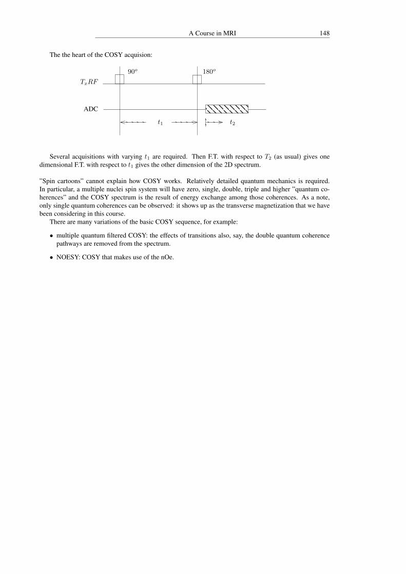
A Course in MRI 148
The the heart of the COSY acquision:
TxRF
ADC
90o 180o
t1 t2
Several acquisitions with varying t1 are required. Then F.T. with respect to T2 (as usual) gives onedimensional F.T. with respect to t1 gives the other dimension of the 2D spectrum.
”Spin cartoons” cannot explain how COSY works. Relatively detailed quantum mechanics is required.In particular, a multiple nuclei spin system will have zero, single, double, triple and higher ”quantum co-herences” and the COSY spectrum is the result of energy exchange among those coherences. As a note,only single quantum coherences can be observed: it shows up as the transverse magnetization that we havebeen considering in this course.
There are many variations of the basic COSY sequence, for example:
• multiple quantum filtered COSY: the effects of transitions also, say, the double quantum coherencepathways are removed from the spectrum.
• NOESY: COSY that makes use of the nOe.

Chapter 14
Functional MRI
Functional MRI (fMRI) refers to the use of MRI for the purpose of detecting active regions in the brain.The detected active regions are often displayed as colors on top of the brain image itself as shown in Figure14.1.
Figure 14.1: Typical fMRI activation maps. The first two images show auditory cortex activation and thethird image shows motor cortex activation. These images are made from EPI BOLD data (explained in thischapter) and the activation maps are overlaid on high resolution T1-weighted spin echo images that wereacquired separately from the BOLD images.
There are two basic approaches to doing measuring brain activation using MRI:
1. Direct measurement of cerebral blood flow (CBF)
(a) by using a gadolinium tracer which is a paramagnetic substance that is given by injection.
(b) the FAIR (Flow Sensitive Alternating Inversion Recovery) technique.
2. The Blood Oxygenation Level Dependent (BOLD) method.
A few experiments were tried with gadolinium before BOLD was discovered. But since it is invasiveand less flexible than BOLD, the method has since been abandoned. (Gadolinium is, however, widely usedto enhance vascularized tumor images in clinical practice.)
FAIR is not as sensitive to activation as BOLD in terms of contrast-to-noise ratio but it is more quanti-tative than BOLD in terms of giving a number for blood flow rates. So it is useful to understand how FAIRworks. Contrast-to-noise (CNR) is defined as
CNR =“max” signal - “min” signal
noise
149
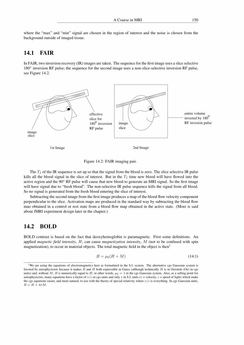
A Course in MRI 150
where the “max” and “min” signal are chosen in the region of interest and the noise is chosen from thebackground outside of imaged tissue.
14.1 FAIR
In FAIR, two inversion recovery (IR) images are taken. The sequence for the first image uses a slice selective180◦ inversion RF pulse; the sequence for the second image uses a non-slice-selective inversion RF pulse,see Figure 14.2.
effective
slice for
RF pulse
o180 inversion
entire volume
inverted by 180
RF invesion pulse
o
������������������
������������������
���������������
���������������
��������������������������������������������������
��������������������������������������������������
����������������������������������������
����������������������������������������
1st Image
sliceimage
2nd Image
image
slice
Figure 14.2: FAIR imaging pair.
The TI of the IR sequence is set up so that the signal from the blood is zero. The slice selective IR pulsekills all the blood signal in the slice of interest. But in the TI time new blood will have flowed into theactive region and the 90o RF pulse will cause that new blood to generate an MRI signal. So the first imagewill have signal due to “fresh blood”. The non-selective IR pulse sequence kills the signal from all blood.So no signal is generated from the fresh blood entering the slice of interest.
Subtracting the second image from the first image produces a map of the blood flow velocity componentperpendicular to the slice. Activation maps are produced in the standard way by subtracting the blood flowmao obtained in a control or rest state from a blood flow map obtained in the active state. (More is saidabout fMRI experiment design later in the chapter.)
14.2 BOLD
BOLD contrast is based on the fact that deoxyhemoglobin is paramagnetic. First some definitions. Anapplied magnetic field intensity, H , can cause magnetization intensity, M (not to be confused with spinmagnetization), to occur in material objects. The total magnetic field in the object is then1
B = µ0(H +M) (14.1)
1We are using the equations of electromagnetics here as formulated in the S.I. system. The alternative cgs Gaussian system isfavored by astrophysicists because it makes B and H both expressible in Gauss (although technically H is in Oersteds (Oe) in cgsunits) and, without M , B is numerically equal to H; in other words, µ0 = 1 in the cgs Gaussian system. Also, as a selling point forastrophysicists, many equations have a factor of v/c in cgs units and only v in S.I. units (v = velocity, c = speed of light) which makethe cgs equations easier, and more natural, to use with the theory of special relativity where v/c is everything. In cgs Gaussian units,B = H + 4πM .

151
where µ0 = 4π× 10−7 Henries/meter (a Henry is a unit of induction in the S.I. system) is the permeabilityof free space2. The amount of magnetization is determined by the suseptibility χ as given by3
M = χH. (14.2)
HereH , M (and laterB) refer to the magnitudes of the vector fields. Note that the magnetic field induction,B, (the quantity that we have been using so far) is related to magnetic field intensity by the permeability µ:
B = µH (14.3)
where µ = µ0µr with µr being the relative permeability. Substituting the definition of suseptibility, Equa-tion (14.2), into Equation (14.1) gives4
B = µ0(1 + χ)H. (14.4)
Note that the definition of permeability in Equation (14.3) leads to µr = (1 + χ). In air, to a high level ofaccuracy5, the applied MRI magnetic field is H = µ0B0. So in the body
B = (1 + χ)B0 (14.5)
and the corresponding spin Larmor frequency is changed by a factor of (1 + χ). So variation of χ overspace leads to T ∗2 MRI signal decay.
Materials may be classified according to their suseptibility:
1. diamagnetic. χ < 0: these materials repel magnetic fields (reduce the intensity). A rod-shaped pieceof diamagnetic material would line up perpendicular to the magnetic field. Most body tissues areslightly diamagnetic.
2. paramagnetic. χ > 0: these materials attract (enhance) magnetic fields. A rod shaped piece ofparamagnetic material will line up parallel to the magnetic field.
3. ferromagnetic. χ� 0 (typically χ > 1000): these materials are composed of magnetized clusters ofatomic magnets that easily line up with the external magnetic field. They stick to magnets.
A “susceptibility gradient” will surround the paramagnetic deoxyhemoglobin molecule. That is, themagnetic field near the deoxyhemoglobin will be higher than it will be further away. So the Larmor fre-quency of the proton spins (usually in water) will be higher near the deoxyhemoglobin than farther away.Suppose we had an infinitely long blood vessel with geometry as shown in Figure 14.3.If Y represents the fraction of oxygenated blood present, then it can be shown that the change in Larmorfrequency from ω0 is given by
∆ωinB = 2π ∆χ0 (1− Y ) ω0
(cos2 θ − 1
3
)(14.6)
inside the cylinder and
∆ωoutB = 2π ∆χ0 (1− Y ) ω0 (rb/r)
2 sin2 θ cos 2φ (14.7)
outside the cylinder where ∆χ0 is the maximum suseptibility difference expected in the presence of fullydeoxygenated blood. The effect of the ∆ωB is to cause spins within a voxel to dephase, thus causing T ∗2signal decay.
2The S.I. unit for B is T (Tesla) while the cgs Gaussian unit is G (Gauss), 1 T = 10000 G. The S.I. unit for H is Amp(turns)/meterwhile the cgs unit is the Oersted; it is apparent why the S.I. unit is favored by engineers: the units of H tell you how many turns ofwire, given some amps, you need to make an electromagnet of a given strength. In S.I. units M still has units of Am−1 but in cgsunits, M has units of emu/cm3 (1 Am−1 = 103 emu/cm3) but 4πM has the units of Gauss. Finally, in the S.I. system, the magneticpolarization is sometimes defined as J = µ0M , so that Equation (14.1) becomes B = µ0H + J .
3The definitions of χ and µ as given in Equations (14.2) and (14.3) are the same in both the S.I. and cgs Gaussian systems.4In cgs Gaussian units, Equation (14.4) is B = (1 + 4πχ)H .5The suseptibility of air is essentially zero.

A Course in MRI 152
Figure 14.3: Blood vessel geometry.
To look at the BOLD phenomenon more closely, remember that the water molecules, and hence thespins, move or diffuse. This motion can lead to “irreversible T ∗2 ”. The effect of diffusion can be classedinto two regemes: dynamic and static averaging.
Dynamic averaging occurs when the diffusive path length during TE is long compared to the susepti-bility gradient, ∂∆ωB
∂r . This occurs, for example, in blood vessels around red blood cells as shown in Figure14.4 or around capillaries or venuoles as shown in Figure 14.5. (Note that there is no BOLD from fullyoxygenated arterial blood.) Dynamic averaging produces irreversible T ∗2 .
Figure 14.4: The diffusion path of a water molecule around and through a red blood cell. The long diffusionpath length relative to the suseptibility gradient leads to dynamic averaging.
Static averaging occurs when the diffusive path length is small compared to the suseptibility gradient,which happens around large blood vessels as shown in Figure 14.6. Static averaging produces reversibleT ∗2 .
Signal loss due to reversible T ∗2 may be recovered as usual with the 180o RF pulse of a spin echosequence.
The definition of what constitutes a large blood vessel increases with increasing field strength, B0,because the suseptibility gradient, represented by ∆ωB , is a function of ω0 = γB0 (see Equation (14.7)).At higher field strengths, static averaging should diminish and be replaced by more sensitive dynamicaveraging around smaller blood vessels.
A third type of BOLD signal is from the so-called “type-2” mechanism. In this case, the blood vesselsand surrounding tissue occupy a similar volume within a voxel. The bulk Larmor frequencies of the protons

153
Figure 14.5: The diffusion path of a water molecule near a capillary. The long diffusion path length relativeto the suseptibility gradient leads to dynamic averaging.
Figure 14.6: The diffusion path of a water molecule near a large blood vessel. The short diffusion pathlength relative to the suseptibility gradient leads to static averaging.
in the blood will be different from the bulk Larmor frequencies in the tissue. So they will go out of andinto phase as shown in Figure 14.7. Type-2 BOLD signal loss is reversible (recoverable) with a spin echosequence.
14.3 Sources of BOLD SignalBOLD signal may come from water molecules in two sources: intravascular and extravascular. And we’veseen that there are reversible and irreversible T ∗2 phenomenon associated with each source:
• Extravascular
– reversible T ∗2 around large blood vessels– irreversible T ∗2 around small blood vessels
• Intravascular
– reversible T ∗2 caused by type-2 BOLD effect– irreversible T ∗2 caused by water molecules moving in and out of red blood cells
Recall that the addition of bipolar diffusion gradients to a sequence attenuated the signal from diffusingwater. These same gradients will kill signal from flowing water. Therefore, a “diffusion sequence” can beused to eliminate intravascular BOLD signal.

A Course in MRI 154
optimal TE
TE
signal sum
in pixel
surrounding tissue
signal
pixel
blood vessel
Figure 14.7: The type-2 BOLD mechanism.
In a similar vein, spin echo sequences may be used to eliminate the BOLD signal from reversible T ∗2effects.
Using a diffusion sequence at 1.5T kills all the BOLD signal which shows that the BOLD signal at 1.5Tmust be intravascular. At higher fields, there is still some BOLD signal from a spin echo experiment andthus some extravascular signal. At very high fields (∼9T) a diffusion sequence doesn’t affect the BOLDsignal at all, implying that all signal at very high Tesla is extravascular.
Using a spin echo sequence for BOLD at 1.5T results in almost no signal showing that most of theBOLD signal at 1.5T is type-2 BOLD. So the BOLD “spatial resolution” at 1.5T is smaller than the pixelsize – no really large blood vessels affect the image.
14.4 The Hemodynamic ResponseThe BOLD signal, being dependent on the amount od deoxyhemoglobin present, depends on 3 factors:
• CBV – Cerebral Blood Volume
• CBF – Cerebral Blood Flow
• CMRO2 – Cerebral Metabolic Rate of O2 consumption
Conceptually, the CBV component appears to be a relatively minor factor, showing itself mostly in its effecton the type-2 BOLD mechanism.
The thing to remember is that the less deoxyhemoglobin present (the more the oxygenated blood) thenthe more the BOLD signal. The presense of deoxyhemoglobin causes suseptibility gradients which de-creases T ∗2 (because of spin dephasing). And, at a fixed TE , the smaller (or shorter) T ∗2 is, the less MRI

155
signal there will be. So the higher the ratio CBF/CMRO2, the higher the BOLD signal. At the begin-ning of the BOLD response, it is believed that the CMRO2 increases at first but that an increase in CBF isresponsible for most of the BOLD signal, see Figure 14.8.
Figure 14.8: The factors in play at the beginning of the BOLD response. The ratio of effects fromCBF/CMRO2 leads to an initial dip in the BOLD signal but, after the dip, the BOLD signal increasesbecause of the large increase in CBF relative to CMRO2.
The system of neurons, their oxygen consumption rate and the resulting smooth muscle response inthe feeding blood vessels may be modeled mathematically with a system of differential equations. Thesedifferential could potentially be used to model the underlying neural system activity that led to the observedhemodynamics. BOLD response functions typically have the general characteristics shown in Figure 14.9.
time
peakto
negative responseEarly
maximumresponse
BOLDresponse
8 to 12 secondswidth
undershoot
Figure 14.9: A typical BOLD response.
The early negative response is generally not seen, but can be detected at higher fields (4T or so). Theundershoot is caused by the elasticity of the blood vessel. It “balloons” up with increased blood flow thenrecoils when the flow is reduced.
The BOLD response is linear with respect to task length up to a saturation point. That is, if the task istwice as long, the width and maximum response will be twice as large. Note that the BOLD, or hemody-namic response, lags behind the actual neural response by a number of seconds and requires a number ofadditional seconds to recover.
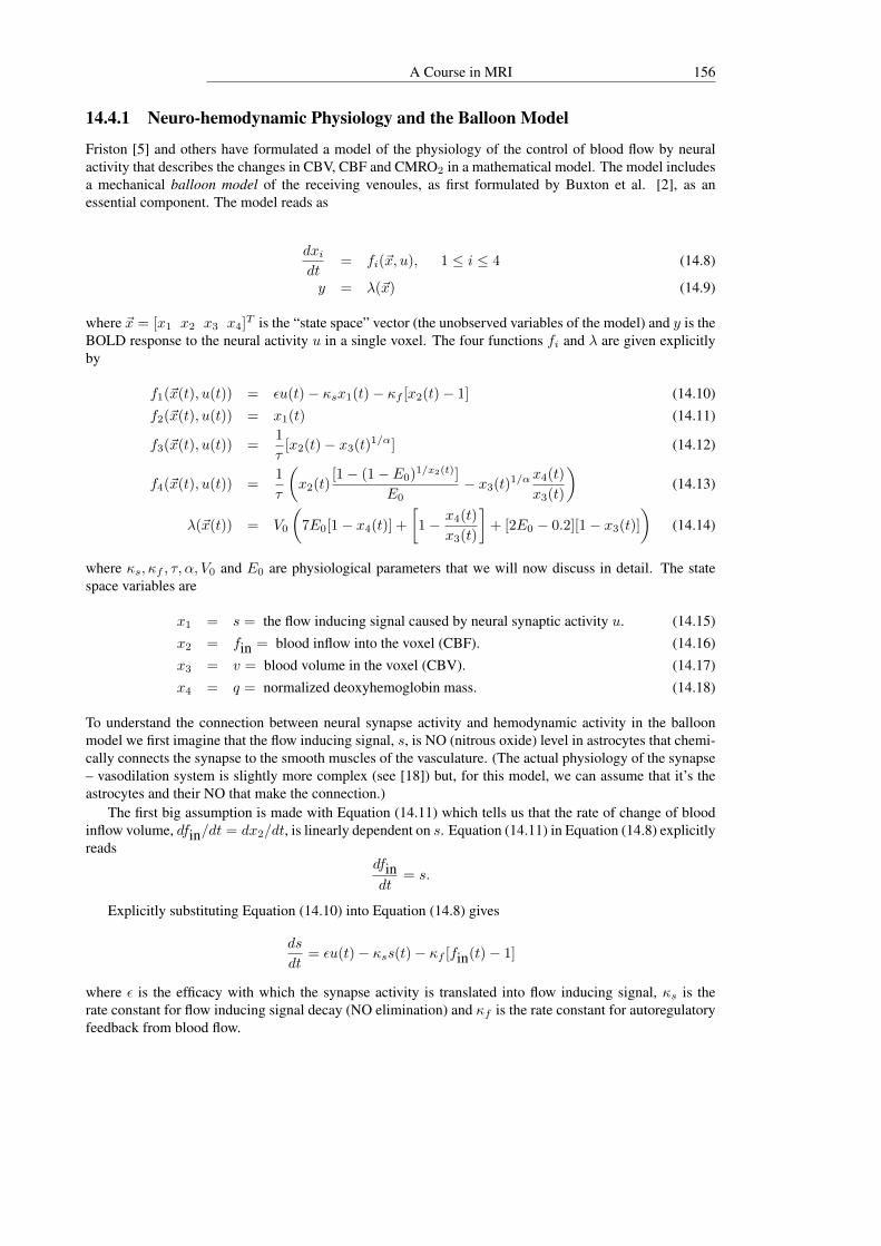
A Course in MRI 156
14.4.1 Neuro-hemodynamic Physiology and the Balloon Model
Friston [5] and others have formulated a model of the physiology of the control of blood flow by neuralactivity that describes the changes in CBV, CBF and CMRO2 in a mathematical model. The model includesa mechanical balloon model of the receiving venoules, as first formulated by Buxton et al. [2], as anessential component. The model reads as
dxidt
= fi(~x, u), 1 ≤ i ≤ 4 (14.8)
y = λ(~x) (14.9)
where ~x = [x1 x2 x3 x4]T is the “state space” vector (the unobserved variables of the model) and y is theBOLD response to the neural activity u in a single voxel. The four functions fi and λ are given explicitlyby
f1(~x(t), u(t)) = εu(t)− κsx1(t)− κf [x2(t)− 1] (14.10)f2(~x(t), u(t)) = x1(t) (14.11)
f3(~x(t), u(t)) =1
τ[x2(t)− x3(t)1/α] (14.12)
f4(~x(t), u(t)) =1
τ
(x2(t)
[1− (1− E0)1/x2(t)]
E0− x3(t)1/αx4(t)
x3(t)
)(14.13)
λ(~x(t)) = V0
(7E0[1− x4(t)] +
[1− x4(t)
x3(t)
]+ [2E0 − 0.2][1− x3(t)]
)(14.14)
where κs, κf , τ, α, V0 and E0 are physiological parameters that we will now discuss in detail. The statespace variables are
x1 = s = the flow inducing signal caused by neural synaptic activity u. (14.15)x2 = fin = blood inflow into the voxel (CBF). (14.16)x3 = v = blood volume in the voxel (CBV). (14.17)x4 = q = normalized deoxyhemoglobin mass. (14.18)
To understand the connection between neural synapse activity and hemodynamic activity in the balloonmodel we first imagine that the flow inducing signal, s, is NO (nitrous oxide) level in astrocytes that chemi-cally connects the synapse to the smooth muscles of the vasculature. (The actual physiology of the synapse– vasodilation system is slightly more complex (see [18]) but, for this model, we can assume that it’s theastrocytes and their NO that make the connection.)
The first big assumption is made with Equation (14.11) which tells us that the rate of change of bloodinflow volume, dfin/dt = dx2/dt, is linearly dependent on s. Equation (14.11) in Equation (14.8) explicitlyreads
dfindt
= s.
Explicitly substituting Equation (14.10) into Equation (14.8) gives
ds
dt= εu(t)− κss(t)− κf [fin(t)− 1]
where ε is the efficacy with which the synapse activity is translated into flow inducing signal, κs is therate constant for flow inducing signal decay (NO elimination) and κf is the rate constant for autoregulatoryfeedback from blood flow.
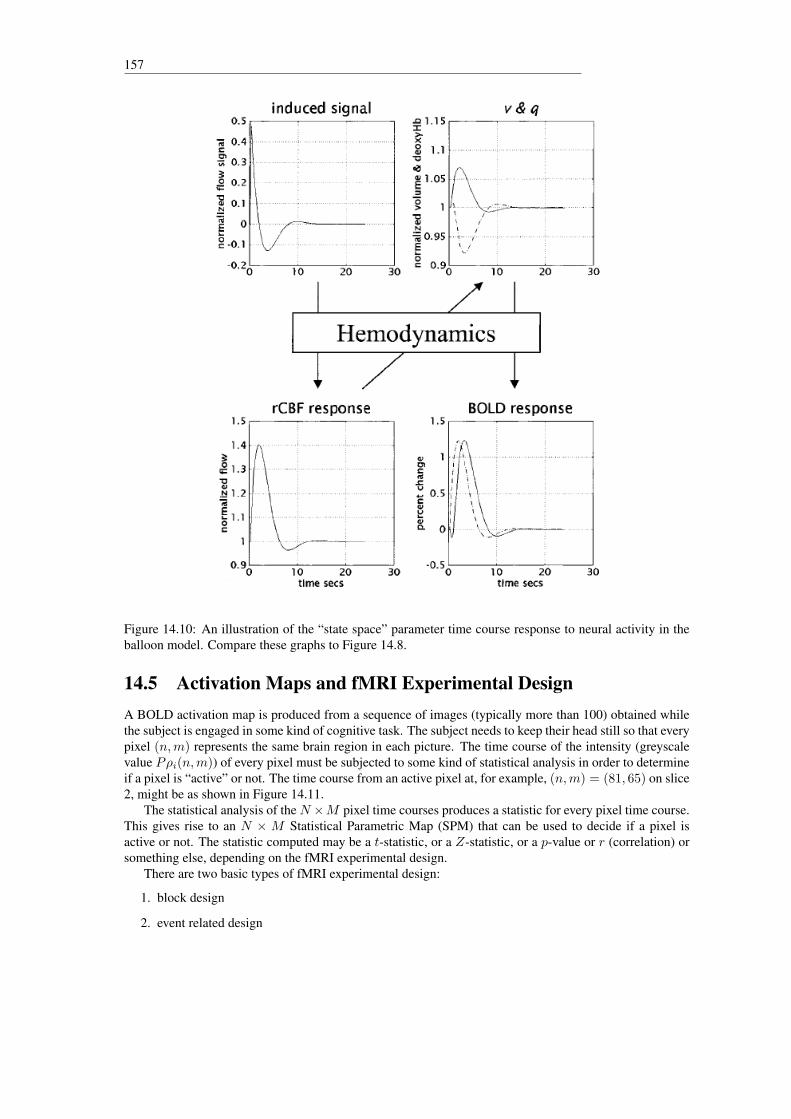
157
Figure 14.10: An illustration of the “state space” parameter time course response to neural activity in theballoon model. Compare these graphs to Figure 14.8.
14.5 Activation Maps and fMRI Experimental DesignA BOLD activation map is produced from a sequence of images (typically more than 100) obtained whilethe subject is engaged in some kind of cognitive task. The subject needs to keep their head still so that everypixel (n,m) represents the same brain region in each picture. The time course of the intensity (greyscalevalue Pρi(n,m)) of every pixel must be subjected to some kind of statistical analysis in order to determineif a pixel is “active” or not. The time course from an active pixel at, for example, (n,m) = (81, 65) on slice2, might be as shown in Figure 14.11.
The statistical analysis of the N ×M pixel time courses produces a statistic for every pixel time course.This gives rise to an N × M Statistical Parametric Map (SPM) that can be used to decide if a pixel isactive or not. The statistic computed may be a t-statistic, or a Z-statistic, or a p-value or r (correlation) orsomething else, depending on the fMRI experimental design.
There are two basic types of fMRI experimental design:
1. block design
2. event related design

A Course in MRI 158
Figure 14.11: An example active pixel time course. The top graph shows when the task is on (e.g. touchingthe fingers of your right hand to your thumb). The time course (from an actual fMRI experiment) is shownon the bottom graph. Note how the signal is very high at first. This is because the spin system is not yetin steady state. As the images are acquired every TR, the spin system will reach a steady state and signalchange will no longer be caused by T1 effects, only by BOLD (and noise sources). The units of the graphare greyscale units.
With the block design, the experimental time course is divided into alternating task and control phases.The signals from the task phase are averaged together (for each pixel) and the signals from the controlphase are averaged together as the first step in activation map computation. Then an unpaired t-test is usedto determine if the signal is significantly different from the signal in the control phase. If it is, then anattribute, such as the average signal difference between task and control, is coded according to a colorbarscheme and the corresponding pixel colored to produce an activation map. A typical colorbar scheme mightbe as shown in Figure 14.12.
The block design is a carryover from old PET6 designs where several minutes are required to make aPET image and typically only one image from each task and control period could be obtained.
When fast measurement techniques like EPI are used, it is possible to obtain an image as fast as every50 ms. (The time between images is the TR for those single shot methods.) So the temporal resolution offMRI is considerably better than the old PET studies.
With the event related design, the temporal resolution of the fMRI experiment may be used to acquiredetailed information about the hemodynamic response. There are two types of event related designs:
1. averaged event related
2. true single event related
With the averaged event related experiment, several blocks of the same event related task are repeated,then averaged together to improve the signal-to-noise ratio. By dividing the event related task into an activephase and a rest phase, the t-test may be used to produce an activation map similarly to the block-design.With this approach, some a priori knowledge of the hemodynamic response must be used to define the twophases.
Another approach to map computation for event related experiments is to correlate an a priori assumedhemodynamic response, as given by a gamma function for example, to the measured response and usethe resulting SPM{r} (SPM of correlation r) to define the activation map. “Gamma functions”, f , that
6Positron Emission Tomography
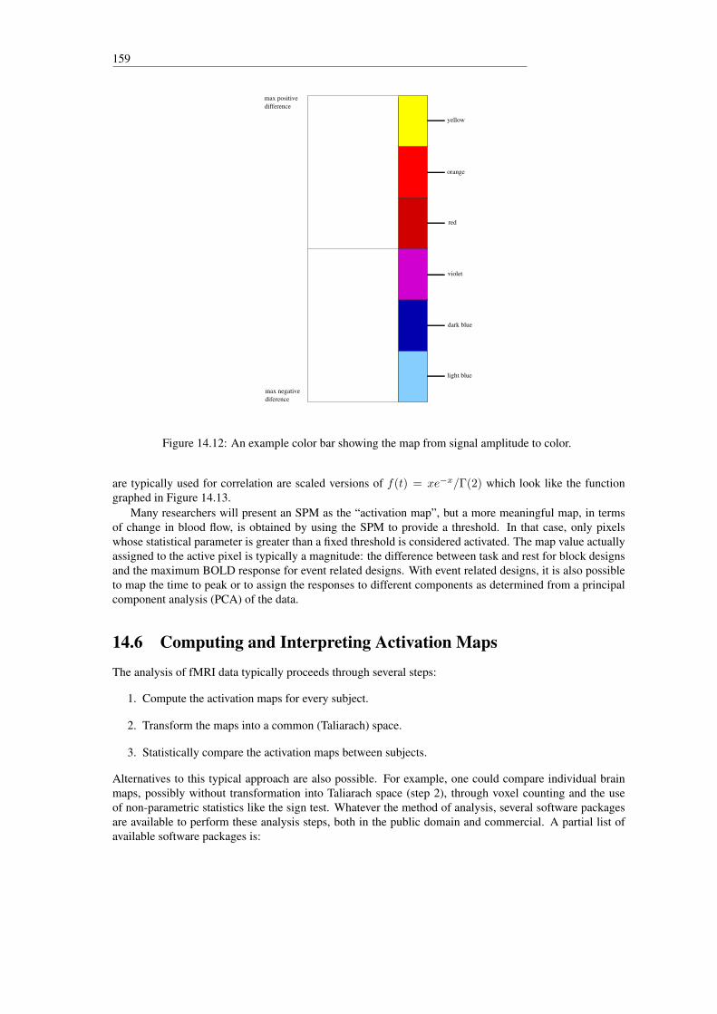
159
orange
yellow
red
violet
dark blue
light blue
difference
max positive
max negative
diference
Figure 14.12: An example color bar showing the map from signal amplitude to color.
are typically used for correlation are scaled versions of f(t) = xe−x/Γ(2) which look like the functiongraphed in Figure 14.13.
Many researchers will present an SPM as the “activation map”, but a more meaningful map, in termsof change in blood flow, is obtained by using the SPM to provide a threshold. In that case, only pixelswhose statistical parameter is greater than a fixed threshold is considered activated. The map value actuallyassigned to the active pixel is typically a magnitude: the difference between task and rest for block designsand the maximum BOLD response for event related designs. With event related designs, it is also possibleto map the time to peak or to assign the responses to different components as determined from a principalcomponent analysis (PCA) of the data.
14.6 Computing and Interpreting Activation Maps
The analysis of fMRI data typically proceeds through several steps:
1. Compute the activation maps for every subject.
2. Transform the maps into a common (Taliarach) space.
3. Statistically compare the activation maps between subjects.
Alternatives to this typical approach are also possible. For example, one could compare individual brainmaps, possibly without transformation into Taliarach space (step 2), through voxel counting and the useof non-parametric statistics like the sign test. Whatever the method of analysis, several software packagesare available to perform these analysis steps, both in the public domain and commercial. A partial list ofavailable software packages is:

A Course in MRI 160
Figure 14.13: The “gamma function” f(t) = xe−x/Γ(2) that is frequently used as an a priori model ofhemodynamic response to an “impulse”.
1. Stimulate. Basic public domain fMRI software. Capable of computing activation maps using a simplet-test or correlation.
2. AFNI. More advanced public domain fMRI software. Uses correlation with an a priori defined hemo-dynamic response function for map computation. It is also effective when used in combination withthe BOLDfold method of computing activation maps.
3. SPM99. Fairly advanced public domain fMRI software based on General Linear Model (GLM)analysis of the timecourse data. Almost every major paper on fMRI reports the use of SPM99 for theanalysis of the data. SPM99 runs on top of Matlab, a commercial software product. The dependenceon Matlab makes SPM99 run slow because many of the routines depend on interpreted, as opposedto compiled, code.
4. EvIdent. Commercial fMRI software from the National Research Council of Canada. It computesmaps using a technique called fuzzy clustering.
5. Brain Voyager. Deluxe commercial fMRI software. Map computation is based on the GLM.
More information, including documentation, on these software packages is available on the University ofSaskatchewan’s fMRI web page at http://prana.usask.ca/∼fMRI. The best way to understandhow the software packages work is to use them (see project at the end of this chapter).
Next, the theory behind the BOLDfold method of map computation, developed by myself and RonBorowsky, is presented. Future versions of this text may give detail on other methods, particularly theGLM approach.
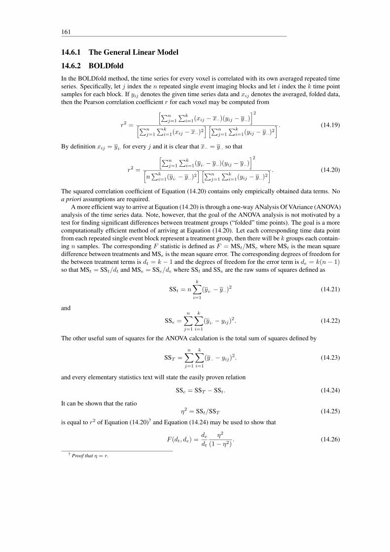
161
14.6.1 The General Linear Model
14.6.2 BOLDfoldIn the BOLDfold method, the time series for every voxel is correlated with its own averaged repeated timeseries. Specifically, let j index the n repeated single event imaging blocks and let i index the k time pointsamples for each block. If yij denotes the given time series data and xij denotes the averaged, folded data,then the Pearson correlation coefficient r for each voxel may be computed from
r2 =
[∑nj=1
∑ki=1(xij − x··)(yij − y··)
]2[∑n
j=1
∑ki=1(xij − x··)2
] [∑nj=1
∑ki=1(yij − y··)2
] . (14.19)
By definition xij = yi· for every j and it is clear that x·· = y·· so that
r2 =
[∑nj=1
∑ki=1(yi· − y··)(yij − y··)
]2[n∑ki=1(yi· − y··)2
] [∑nj=1
∑ki=1(yij − y··)2
] . (14.20)
The squared correlation coefficient of Equation (14.20) contains only empirically obtained data terms. Noa priori assumptions are required.
A more efficient way to arrive at Equation (14.20) is through a one-way ANalysis Of VAriance (ANOVA)analysis of the time series data. Note, however, that the goal of the ANOVA analysis is not motivated by atest for finding significant differences between treatment groups (“folded” time points). The goal is a morecomputationally efficient method of arriving at Equation (14.20). Let each corresponding time data pointfrom each repeated single event block represent a treatment group, then there will be k groups each contain-ing n samples. The corresponding F statistic is defined as F = MSt/MSe where MSt is the mean squaredifference between treatments and MSe is the mean square error. The corresponding degrees of freedom forthe between treatment terms is dt = k − 1 and the degrees of freedom for the error term is de = k(n− 1)so that MSt = SSt/dt and MSe = SSe/de where SSt and SSe are the raw sums of squares defined as
SSt = n
k∑i=1
(yi· − y··)2 (14.21)
and
SSe =
n∑j=1
k∑i=1
(yi· − yij)2. (14.22)
The other useful sum of squares for the ANOVA calculation is the total sum of squares defined by
SST =
n∑j=1
k∑i=1
(y·· − yij)2. (14.23)
and every elementary statistics text will state the easily proven relation
SSe = SST − SSt. (14.24)
It can be shown that the ratioη2 = SSt/SST (14.25)
is equal to r2 of Equation (14.20)7 and Equation (14.24) may be used to show that
F (dt, de) =dedt
η2
(1− η2). (14.26)
7 Proof that η = r.

A Course in MRI 162
Therefore the direct BOLDfold correlation analysis and the ANOVA calculation provide the same informa-tion about the voxel intensity time series. The ANOVA approach eliminates an explicit computation of thenumerator of Equation (14.20).
The actual implementation of BOLDfold is a variation on the above scheme in which the data yijwere replaced by data corrected for baseline drift via linear regression. That is, the linear effect of the“confounding” variable time, tij , was removed through defining the corrected data to be zij = yij − αtijwhere α is the slope of the baseline drift found through a linear regression on all considered data points yij .Therefore, the computation of F (and subsequently η via Equation (14.26)) is equal to the F associatedwith an ANalysis of COVARiance (ANCOVA) of the time series data slotted into k treatment groups with nsamples per group. The General Linear Model design matrix for the determination of the average BOLDfoldresponse is identical to the design matrix for an ANCOVA analysis of the same data. However, as with theANOVA approach, the ANCOVA approach used here is not indented to be a classical ANCOVA statisticalanalysis of the data but, instead, is an efficient means for computing the correlation of the time series datawith its own averaged time course. This fine point is important for the subsequent interpretation of any“type I error” (p value) associated with either the F or r statistic.
More complex versions of the BOLDfold procedure may be obtained by projecting low frequency har-monics out of the time course data [3]. Such processing may be helpful in eliminating physiologicallyproduced confounds from the data if such confounds happen to occur at an integer multiple of the experi-ment’s repetition period. In general, the probability of such a coincidence must be low and our ANCOVAapproach for projecting out linear drift should normally be all that is required.
The visibility (magnitude) values, a, used in the activation map are
a = (maxizi· −min
izi·)/min
izi·. (14.27)
The visibility a is multiplied by -1 if mini zi· occurred before maxi zi·. The negative visibility values wouldthen represent possible deactivated regions or, more likely, “activations” due to motion. The visibilities arethresholded at a pre-specified η level; that is, if η for a given voxel were below the threshold, then a is setto zero.
Let ti = yi· − y·· and Tij = yij − y··. Then from Equation (14.20)
r2 =
[∑nj=1
∑ki=1 tiTij
]2[n∑k
i=1 t2i
] [∑nj=1
∑ki=1 T
2ij
]and from Equation (14.25)
η2 =n∑k
i=1 t2i∑n
j=1
∑ki=1 T
2ij
.
Therefore
r2 = η2
[∑nj=1
∑ki=1 tiTij
]2[n∑k
i=1 t2i
]2 .
Sincen∑
j=1
k∑i=1
tiTij =
k∑i=1
ti
n∑j=1
Tij
it follows that
r = η(1/n)
∑ki=1 ti
(∑nj=1 Tij
)∑k
i=1 t2i
.
But
(1/n)n∑
j=1
Tij = (1/n)n∑
j=1
(yij − y··) = (1/n)
n∑j=1
yij
− y·· = yi· − y·· = ti
so r = η.

163
14.7 More About the Source of the fMRI SignalBOLD based fMRI is an indirect way of measuring brain activity. BOLD is based on blood flow changes inbrain regions that are active. The blood flow changes are caused by the physiologic demands of the neuronsbut BOLD fMRI maps do not show neural activity directly. In fact, the BOLD response is very slow - ittakes several seconds to build up to a level where it causes and observable change in the MRI signal, and ittakes several seconds to decline as we saw in §14.4.1 (see Figure 14.9). And, of course, the cognitive taskassociated with and observable BOLD MRI signal must be relatively long in duration.
Methods for measuring neural activity directly have been either invasive, like surgically implanted elec-trodes, or very expensive like magnetoenchaphalography (MEG). An exception is electroenchaphalography(EEG). It is useful to understand a little about how these other methods work because many researchers nowuse fMRI in combination with these other methods. To see how these other methods of measuring neuralactivity work, let’s first consider how a neuron works.
14.7.1 Neuron Physiology – In BriefNeural activity is electrical (see Figure 14.14). A neuron at rest maintains a balance of various ion concen-trations inside the cell through a variety of mechanisms as shown in Figure 14.15. Then the neuron fires;the membrane channels open and the interior potential changes as shown in Figure 14.16.
Figure 14.14: The electrical current in the neuron (in the axon in particular) is the result of ion flow.

A Course in MRI 164
kept mostly
interior potential
balance of electrostaticof ï70mv due primarily to
and diffusion forcesacross the cell membrane
for ïCl
+K
ïCl
inside by membranepumps
Figure 14.15: A neuron at rest, showing the interior ion distributions.
14.7.2 The Relationship Between Neural Activity and BOLDLogothetis et al. [24] report that the BOLD response is to local field potentials (LFPs). Logothetis et al.measured both multi-unit activity (MUA) and LFP while doing an fMRI BOLD measurement on monkeys.According to Logothetis et al. MUA corresponds to the output of a neural population; LFP correspondsmostly to a weighted average of synchronized dendro-somatic components of the input signals of a neuralpopulation. Logothetis et al. found that BOLD correlated with LFP more than MUA. They also recordedsingle unit activity and found it to behave similarly to MUA. A typical response is shown in Figure 14.17.
After linear systems modeling, Logothetis et al. describe the BOLD response to be a low-pass filteredversion of total neural activity.
14.7.3 EEG and MEGSo what if we want to map more detailed neural activity? The electrode methods are invasive. EEG canmeasure electrical potential on the scalp but not inside the brain. Crude 3D reconstruction of electricalpotential inside the brain from EEG data is possible if many assumptions are made but the extrapolation of2D scalp data to 3D brain data is essentially and ill-posed problem.
Associated with all electrical current (including ion flow in axons) is a magnetic field by the right handrule as shown in Figure 14.18.
In other words, neurons generate their own magnetic field. But the field is very small. To measure theneural magnetic fields directly requires a very sensitive magnetometer called a SQUID (SuperconductingQuantum interference Device). Being superconducting, SQUID needs to be cooled to near absolute zero byliquid helium. An MEG device uses several SQUIDS place around the head to measure the neural activity.The set-up is roughly as shown in Figure 14.19.
The MEG must also be placed in a tightly shielded room to prevent commercial RF ad other externalelectrical activity from generating signal in the SQUIDS. MEGS are expensive, about an order of magnitudemore expensive than and MRI and you still have the ill posed problem of connecting measure scalp magneticactivity to a 3D brain map.
So both EEG and MEG are based on measuring something on the 2D surface of the scalp – on the
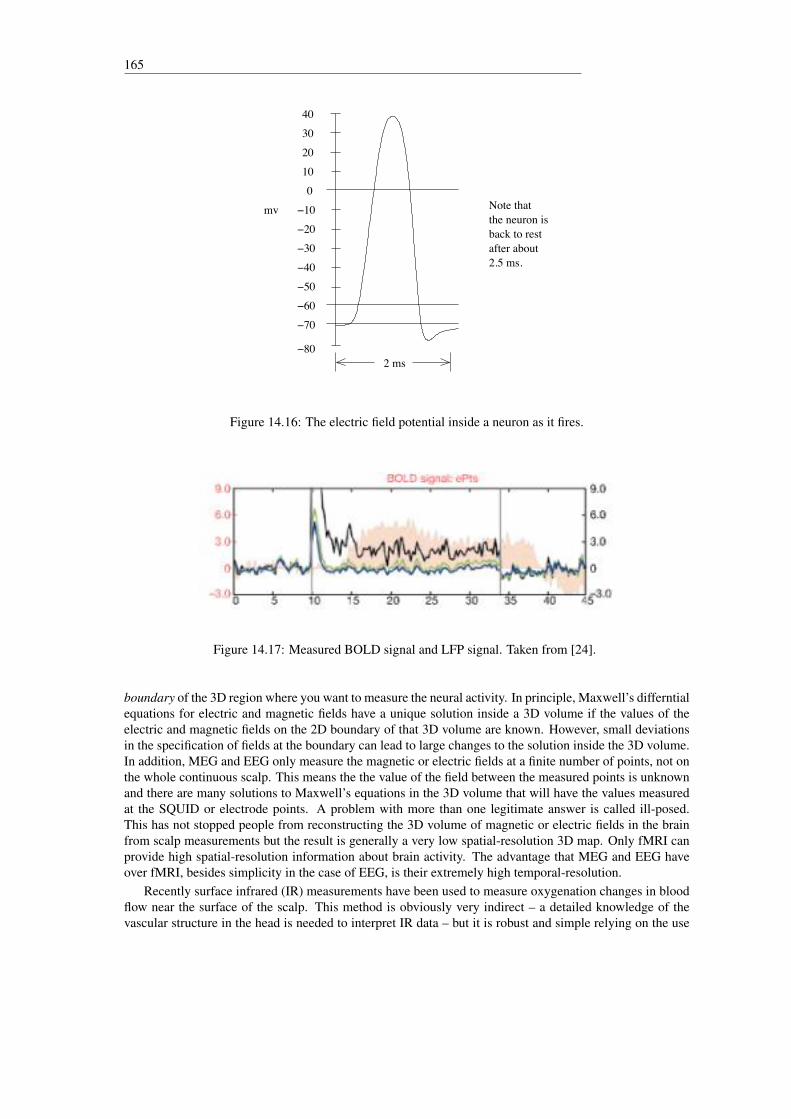
165
40
30
20
10
ï10
ï30
ï40
ï60
ï80
ï20
ï50
ï70
0
mv
2 ms
Note that the neuron isback to restafter about2.5 ms.
Figure 14.16: The electric field potential inside a neuron as it fires.
Figure 14.17: Measured BOLD signal and LFP signal. Taken from [24].
boundary of the 3D region where you want to measure the neural activity. In principle, Maxwell’s differntialequations for electric and magnetic fields have a unique solution inside a 3D volume if the values of theelectric and magnetic fields on the 2D boundary of that 3D volume are known. However, small deviationsin the specification of fields at the boundary can lead to large changes to the solution inside the 3D volume.In addition, MEG and EEG only measure the magnetic or electric fields at a finite number of points, not onthe whole continuous scalp. This means the the value of the field between the measured points is unknownand there are many solutions to Maxwell’s equations in the 3D volume that will have the values measuredat the SQUID or electrode points. A problem with more than one legitimate answer is called ill-posed.This has not stopped people from reconstructing the 3D volume of magnetic or electric fields in the brainfrom scalp measurements but the result is generally a very low spatial-resolution 3D map. Only fMRI canprovide high spatial-resolution information about brain activity. The advantage that MEG and EEG haveover fMRI, besides simplicity in the case of EEG, is their extremely high temporal-resolution.
Recently surface infrared (IR) measurements have been used to measure oxygenation changes in bloodflow near the surface of the scalp. This method is obviously very indirect – a detailed knowledge of thevascular structure in the head is needed to interpret IR data – but it is robust and simple relying on the use

A Course in MRI 166
Magnetic Field
Figure 14.18: The magnetic field around an axon follows the right hand rule.
dewar full of
liquid H2
SQUIDS
Figure 14.19: MEG setup.
of cheap diodes for measurement.It was hoped that MRI might be used to measure the magnetic activity of neurons directly since the
neural magnetic field should lead to spin dephasing, see Figure 14.20. So the signal from a voxel containingactive neurons should decrease — opposite to what happens in BOLD where spins are less out of phase inthe presence of oxyhemoglobin. Xiong et al. [27] claimed, in a method they called msMRI for magneticsource MRI, to measure a 1%-5% change in the MRI signal caused by neural magnetoc fields. In spiteof the success reported by Xiong et al. we, here at the University of Saskatchewan, have not been able toreproduce their results. Others have also not been able to replicate the msMRI approach and evidence hasaccumulated that msMRI may not be possible in general, although other positive reports have appeared. Foran example of negative results see the paper by Parkes et al. [15] in which a failure to reproduce Xiong etal.’s results, as well as another approach to msMRI that we have not discussed here, is reported.
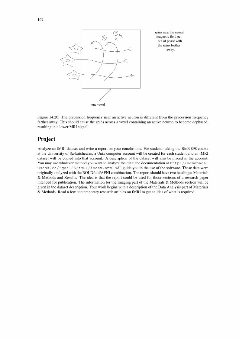
167
spins near the neural
magnetic field get
the spins further
out of phase with
away.
one voxel
Figure 14.20: The precession frequency near an active neuron is different from the precession frequencyfarther away. This should cause the spins across a voxel containing an active neuron to become dephased,resulting in a lower MRI signal.
ProjectAnalyze an fMRI dataset and write a report on your conclusions. For students taking the BioE 898 courseat the University of Saskatchewan, a Unix computer account will be created for each student and an fMRIdataset will be copied into that account. A description of the dataset will also be placed in the account.You may use whatever method you want to analyze the data; the documentation at http://homepage.usask.ca/˜ges125/fMRI/index.html will guide you in the use of the software. These data wereoriginally analyzed with the BOLDfold/AFNI combination. The report should have two headings: Materials& Methods and Results. The idea is that the report could be used for those sections of a research paperintended for publication. The information for the Imaging part of the Materials & Methods section will begiven in the dataset description. Your work begins with a description of the Data Analysis part of Materials& Methods. Read a few contemporary research articles on fMRI to get an idea of what is required.

A Course in MRI 168
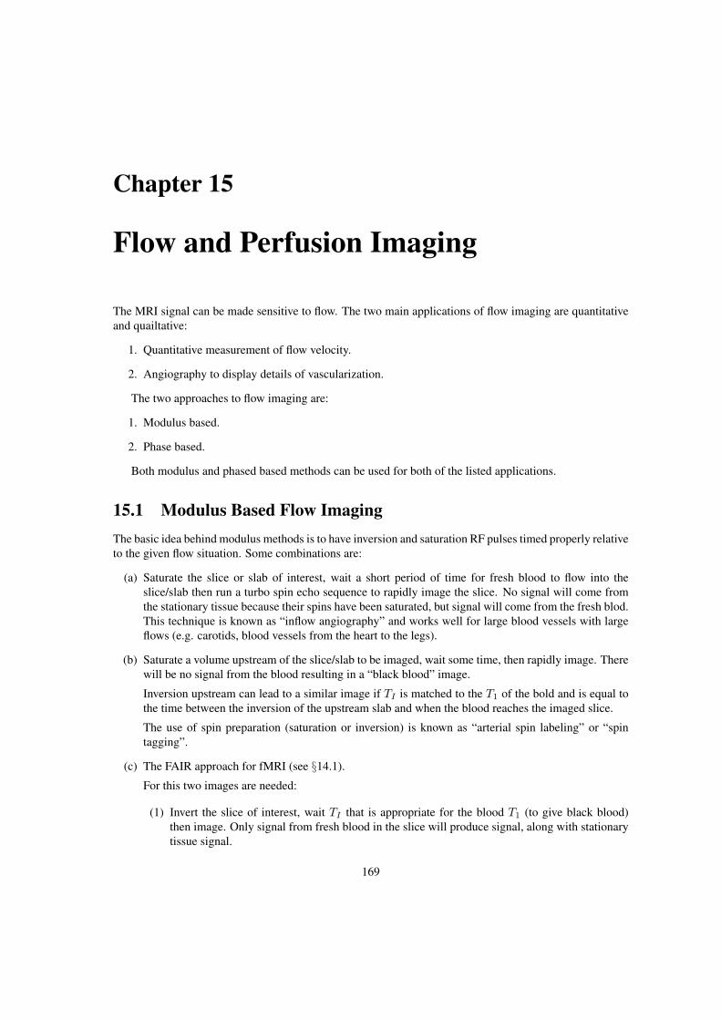
Chapter 15
Flow and Perfusion Imaging
The MRI signal can be made sensitive to flow. The two main applications of flow imaging are quantitativeand quailtative:
1. Quantitative measurement of flow velocity.
2. Angiography to display details of vascularization.
The two approaches to flow imaging are:
1. Modulus based.
2. Phase based.
Both modulus and phased based methods can be used for both of the listed applications.
15.1 Modulus Based Flow ImagingThe basic idea behind modulus methods is to have inversion and saturation RF pulses timed properly relativeto the given flow situation. Some combinations are:
(a) Saturate the slice or slab of interest, wait a short period of time for fresh blood to flow into theslice/slab then run a turbo spin echo sequence to rapidly image the slice. No signal will come fromthe stationary tissue because their spins have been saturated, but signal will come from the fresh blod.This technique is known as “inflow angiography” and works well for large blood vessels with largeflows (e.g. carotids, blood vessels from the heart to the legs).
(b) Saturate a volume upstream of the slice/slab to be imaged, wait some time, then rapidly image. Therewill be no signal from the blood resulting in a “black blood” image.
Inversion upstream can lead to a similar image if TI is matched to the T1 of the bold and is equal tothe time between the inversion of the upstream slab and when the blood reaches the imaged slice.
The use of spin preparation (saturation or inversion) is known as “arterial spin labeling” or “spintagging”.
(c) The FAIR approach for fMRI (see §14.1).
For this two images are needed:
(1) Invert the slice of interest, wait TI that is appropriate for the blood T1 (to give black blood)then image. Only signal from fresh blood in the slice will produce signal, along with stationarytissue signal.
169
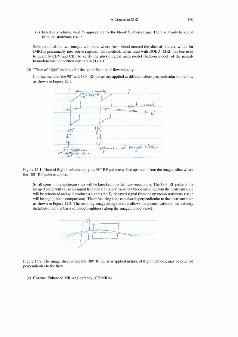
A Course in MRI 170
(2) Invert in a volume, wait TI appropriate for the blood T1, then image. There will only be signalfrom the stationary tissue.
Subtraction of the two images will show where fresh blood entered the slice of interest, which forfMRI is presumably into active regions. This method, when used with BOLD fMRI, has bee usedto quantify CBV and CBF to verify the physiological math model (balloon model) of the neural-hemodynamic connection covered in §14.4.1.
(d) “Time of flight” methods for the quantification of flow velocity.
In these methods the 90◦ and 180◦ RF pulses are applied at different slices perpendicular to the flowas shown in Figure 15.1.
Figure 15.1: Time of flight methods apply the 90◦ RF pulse to a slice upstream from the imaged slice wherethe 180◦ RF pulse is applied.
So all spins in the upstream slice will be knocked into the transverse plane. The 180◦ RF pulse at theimaged plane will cause no signal from the stationary tissue but blood arriving from the upstream slicewill be refocused and will produce a signal (the T ∗2 decayed signal from the upstream stationary tissuewill be negligible in comparison). The refocusing slice can also be perpendicular to the upstream sliceas shown in Figure 15.2. The resulting image along the flow allows the quantification of the velocitydistribution on the basis of blood brightness along the imaged blood vessel.
Figure 15.2: The image slice, where the 180◦ RF pulse is applied in time of flight methods, may be orientedperpendicular to the flow.
(e) Contrast Enhanced MR Angiography (CE-MRA).

171
In this method, a Gadolinium (Gd) based contrast agent is injected into the patient. The Gd-basedagent lowers the T1 of the blood by offering more realxation pathways. Therefore blood will appearbrighter in Gd enhanced images than in regular images. Subtraction of a regular image from a Gd-enhanced image will give an angiogram.
15.1.1 Display of angiogramsOne a volume dataset that shows only signal from blood in arteries is produced (e.g. by subtraction of Gd-enhanced and unenhanced images), then the angiogram may be viewed using the visualization technique ofMaximum Intensity Projection (MIP). With MIP an image is produced for a number of rotation angles (ofthe volume) by producing an image, for each angle, in which the pixel value is taken as the maximum voxelvalue on a line perpendicular to the image through the volume. MIP angiograms can be quite spectacularas shown in Figure 15.3.
Figure 15.3: An MRI MIP angiogram ripped-off from the interweb.
15.2 Phase-based Flow ImagingThe basic principles behind phase-based imaging may be summarized in the following points:
• Gradient waveforms having a zero zero-order moment,∫G(t) dt = 0, (15.1)
will not affect the signal from stationary tissue but will produce signals sensitive to velocity. Figure15.4) shows the classic bipolar waveform whose zero-order moment is zero.
Figure 15.4: The bipolar gradient waveform has∫G(t) dt = 0.

A Course in MRI 172
• Gradient waveforms having zero first-order moment,∫G(t) t dt = 0, (15.2)
will be velocity insensitive (see Figure 15.5).
Figure 15.5: An example gradient waveform with zero first order moment∫G(t) t dt = 0.
So gradient waveforms inserted in the imaging sequence may be used to produce velocity sensitiveimages and velocity insensitive images. Subtraction then leads to angiograms.
Phase-based flow imaging is also very ideal for velocity quantification. The phase of the transversemagnetization can be made proportional to the velocity as follows.
• Assume zero acceleration. (It is possible to quantify any motion; we assume constant velocity herefor pedagogical purposes.) Also assume motion in the x direction.
• Assume a gradient waveform of the type shown in Figure 15.6.
Figure 15.6: Parametrized gradient waveform.
We want to know what the phase of the spins at voxel ~p at time tm is. Denote that phase by ϕ(~p, tm) (inthe rotating frame). Phase is angular position in the rotating frame. If the spins precess at frequency ω(t)in the rotating frame then
ϕ(~p, tm) =
∫ω(~p, t) dt. (15.3)
The precession frequency of the spin that ends up at ~p at the time tm is given by
ω(~p, t) = γ x(~p, t) Gx(t) (15.4)
where x(~p, t) denotes the position of the spin that ends up at position ~p at the time tm.Let te be a time before T− τ
2 (when the gradients are first turned on, see Figure 15.6), and let xe = x(te).Then
x(~p, t) = xe + v(t− te) (15.5)
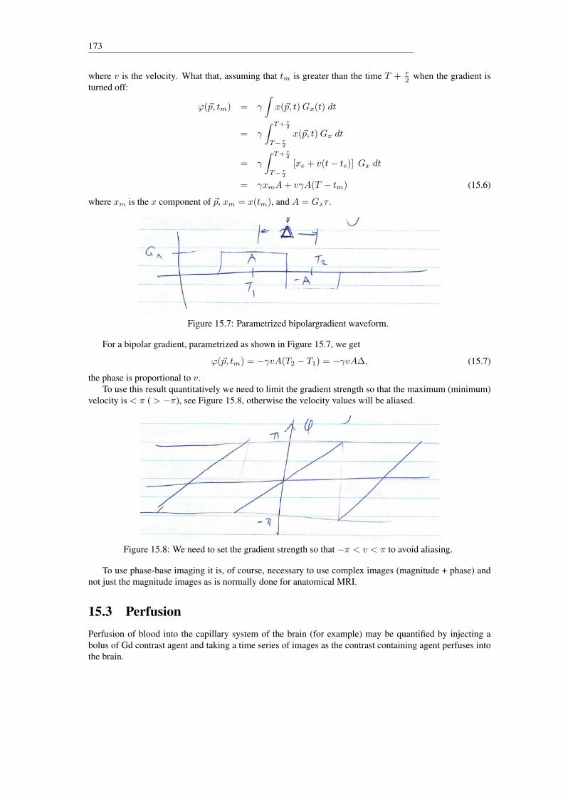
173
where v is the velocity. What that, assuming that tm is greater than the time T + τ2 when the gradient is
turned off:
ϕ(~p, tm) = γ
∫x(~p, t)Gx(t) dt
= γ
∫ T+ τ2
T− τ2x(~p, t)Gx dt
= γ
∫ T+ τ2
T− τ2[xe + v(t− te)] Gx dt
= γxmA+ vγA(T − tm) (15.6)
where xm is the x component of ~p, xm = x(tm), and A = Gxτ .
Figure 15.7: Parametrized bipolargradient waveform.
For a bipolar gradient, parametrized as shown in Figure 15.7, we get
ϕ(~p, tm) = −γvA(T2 − T1) = −γvA∆, (15.7)
the phase is proportional to v.To use this result quantitatively we need to limit the gradient strength so that the maximum (minimum)
velocity is < π ( > −π), see Figure 15.8, otherwise the velocity values will be aliased.
Figure 15.8: We need to set the gradient strength so that −π < v < π to avoid aliasing.
To use phase-base imaging it is, of course, necessary to use complex images (magnitude + phase) andnot just the magnitude images as is normally done for anatomical MRI.
15.3 PerfusionPerfusion of blood into the capillary system of the brain (for example) may be quantified by injecting abolus of Gd contrast agent and taking a time series of images as the contrast containing agent perfuses intothe brain.

A Course in MRI 174
Each time-series image is subtracted from a base (non-contrast enhanced) image taken prior to bolusinjection to produce time series images that show the concentration of contrast agent over time, see Figure15.9.
Figure 15.9: At one pixel in the subtracted time series images we might track bolus perfusion through theimage intensity of that pixel.
A math model of the perfusion into tissue can be fit to a curve like that shown in Figure 15.9 to quantifythe perfusion and to produce a perfusion map.
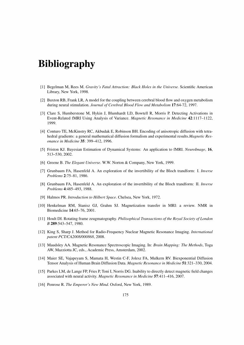
Bibliography
[1] Begelman M, Rees M. Gravity’s Fatal Attraction: Black Holes in the Universe. Scientific AmericanLibrary, New York, 1998.
[2] Buxton RB, Frank LR, A model for the coupling between cerebral blood flow and oxygen metabolismduring neural stimulation. Journal of Cerebral Blood Flow and Metabolism 17:64-72, 1997.
[3] Clare S, Humberstone M, Hykin J, Blumhardt LD, Bowtell R, Morris P. Detecting Activations inEvent-Related fMRI Using Analysis of Variance. Magnetic Resonance in Medicine 42:1117–1122,1999.
[4] Conturo TE, McKinstry RC, Akbudak E, Robinson BH. Encoding of anisotropic diffusion with tetra-hedral gradients: a general mathematical diffusion formalism and experimental results.Magnetic Res-onance in Medicine 35: 399–412, 1996.
[5] Friston KJ. Bayesian Estimation of Dynamical Systems: An application to fMRI. NeuroImage, 16,513–530, 2002.
[6] Greene B. The Elegant Universe. W.W. Norton & Company, New York, 1999.
[7] Grunbaum FA, Hasenfeld A. An exploration of the invertibility of the Bloch trandform: I. InverseProblems 2:75–81, 1986.
[8] Grunbaum FA, Hasenfeld A. An exploration of the invertibility of the Bloch trandform: II. InverseProblems 4:485–493, 1988.
[9] Halmos PR. Introduction to Hilbert Space. Chelsea, New York, 1972.
[10] Henkelman RM, Stanisz GJ, Grahm SJ. Magnetization transfer in MRI: a review. NMR inBiomedicine 14:65–76, 2001.
[11] Hoult DI. Rotating frame zeugmatography. Philisophical Transactions of the Royal Society of LondonB 289:543–547, 1980.
[12] King S, Sharp J. Method for Radio-Frequency Nuclear Magnetic Resonance Imaging. Internationalpatent PCT/CA2008/000868, 2008.
[13] Maudsley AA. Magnetic Resonance Spectroscopic Imaging. In: Brain Mapping: The Methods, TogaAW, Mazziotta JC, eds., Academic Press, Amsterdam, 2002.
[14] Maier SE, Vajapeyam S, Mamata H, Westin C-F, Jolesz FA, Mulkern RV. Biexponential DiffusionTensor Analysis of Human Brain Diffusion Data. Magnetic Resonance in Medicine 51:321–330, 2004.
[15] Parkes LM, de Lange FP, Fries P, Toni I, Norris DG. Inability to directly detect magnetic field changesassociated with neural activity. Magnetic Resonance in Medicine 57:411–416, 2007.
[16] Penrose R. The Emperor’s New Mind. Oxford, New York, 1989.
175
A Course in MRI 176
[17] Penrose R. Shadows of the Mind. Oxford, New York, 1994.
[18] Peppiatt C, Attwell D. Feeding the brain. Nature 431, 137-138, 2004.
[19] Sharp J, King S. RF Based Spatially Selective Excitation in MRI. International patentPCT/CA2008/000866, 2008.
[20] Sharp J, King S. MRI using radiofrequency magnetic field phase gradients. Magnetic Resonance inMedicine 63:151–161, 2010.
[21] Slichter CP. Principles of Magnetic Resonance. Springer, Heidelberg, 1996.
[22] Song AW, Guo H, Truong T-R. Single-shot ADC imaging for fMRI. Magnetic Resonance in Medicine57:417–422, 2007.
[23] Suggs JW. Organic Chemistry. Barron’s, New York, 2002.
[24] Logothetis NK, Pauls J, Augath M, Trinath T, Oeltermann A. Neurophysiologcal investigation of thebasis of the fMRI signal. Nature 412:150–157, 2001.
[25] Macomber RS. A Complete Introduction to Modern NMR Spectroscopy. John Wiley & Sons, NewYork, 1998.
[26] Wilczek F. Precision precession. Nature 410:28–29, 2001.
[27] Xiong J, Fox PT, Gao JH. Directly mapping field effect of neuronal activity by magnetic resonanceimaging. Human Brain Mapping 20:41–49, 2003

Appendix A
Math Needed for this Book
A.1 VectorsA vector is a quantity with magnitude and direction. So, it refers to quantities in spaces having dimension2 or higher. There are a number of ways of representing vectors:
1. As ordered n-tuples:~a = (a1, a2, a3, . . . , an)
(If the commas were removed, the n-tuple would be known as a row vector.) In 2D the corresponding2-tuple is written as
~a = (a1, a2)
2. As Column Vectors:
~a =
(a1
a2
)in 2D.
The column vector is longer in higher dimensions. The use of column vectors is convenient forcalculations with matrices.
3. As Combinations of Multiples of Orthogonal Unit Vectors:
In 2D:~a = a1~ı+ a2~
In 3D:~a = a1~ı+ a2~+ a3
~k
The unit vectors,~ı,~,~k whose length is 1, visually look like:In 2D:
~ı (x)
~ (y)
In 3D:~k (z)
~ı (x)
~ (y)
In every case the numbers a1, a2, a3, . . ., etc. represent the components of the vector~a. The componentsprovide a convenient way of decomposing the vector. The length of the vector is given by a generalized
177

A Course in MRI 178
Pythagoras formula. The length of a vector ~a is represented by ||~a|| and computed with, for example, theformula
||~a|| =√a2
1 + a22 + a2
3
in 3D. The square of the length of a vector is just the sum of squares of the vector’s components.Examples:In 2D:
~a = (1, 2) =
(12
)= 1~ı+ 2~
1
2
3
4
1 2 3 4
y
x~
~ı
2~
1~ı
In 3D:
~a = (2, 3, 2) =
232
= 2~ı+ 3~+ 2~k
so a1 = 2, a2 = 3, a3 = 2.
4
3
2
1
1 2 3 4
43
21
x
y
z
a3a1
a2
~ı ~
~k
Notational conventions: The vector itself (as opposed to its components) has been represented above by aletter with an arrow over it as in ~a. This notation has not been used consistently in this course; for example

179
in the chapter on quantum mechanics no arrow is used. The inconsistency is deliberate so that the notationis roughly consistent with the existing literature. Another common convention is to denote vectors withboldface as in a. However, boldface is difficult to produce on a blackboard.
Terminology: There are vectors and scalars. The student may be familiar with the case where the scalarsare real numbers, that is, when n-dimensional vectors are n-tuples of real numbers, R. But the scalars canalso be complex numbers, C. If the scalars are real, the set of all n-dimensional vectors is denoted as Rn.If the scalars are complex, the set of all n-dimensional vectors is denoted by Cn.
A.2 Inner ProductsAn inner product of 2 vectors, a and b is the sum of the product of their components. (Note that the arrowhas been dropped here.) The inner product is written a couple of ways:
1. a · b
2. 〈a, b〉 or 〈a|b〉
The inner product is also called the dot product when the vector space is finite dimensional. In generalthe inner product is defined by:
a · b = 〈a, b〉 = a1b1 + a2b2 + a3b3 + . . . anbn
In 2D:〈a, b〉 = a1b2 + a2b2
In 3D:〈a, b〉 = a1b1 + a2b2 + a3b3
Examples:In 2D:
Find the inner product of:
a =
(12
)b =
(34
)To find the inner product of a and b, remember that:
a =
(a1
a2
)b =
(b1b2
)Then
〈a, b〉 = (1× 3) + (2× 4) = 11

A Course in MRI 180
In 3D:Find the inner product of:
~a =
121
~b =
212
〈a, b〉 = (1× 2) + (2× 1) + (1× 2) = 6
Terminology: Inner products map pairs of vectors to a scalar.
Definition: The transpose of a column vector a is a row vector denoted by aT and is defined as follows:
If a =
a1
a2
...an
then aT = (a1, a2, . . . an). For example, in 2D if a =
(12
)then aT = (1 2), if
a =
(35
)then aT = (3 5). In 3D if a =
125
then aT = (1 2 5). Notice that no commas have been
used between components: this is the row vector notation mentioned in Section A.1 on vectors.The transpose makes it possible to represent inner product in a matrix multiplication way. Specifically:
〈a, b〉 = aT b
Examples:In 2D:
The inner product of
a =
(12
)b =
(35
)is given by
〈a, b〉 = aT b = (1 2)
(35
)= 13
The way to do the calculation in your head is to mentally flip the row vector into the column vector andmatch with the given column vector, multiply the matching components and add the results down the col-umn. This is the usual matrix multiplication procedure.
A.3 MatricesA matrix is an n ×m array of numbers or scalars. We only need to worry about n × n, n × 1 and 1 × nmatrices in the course. In general, an n×m matrix has n rows and m columns. So an n× 1 matrix (whichhas n rows and 1 column) is a column vector and a 1× n matrix is a row vector.

181
Examples:In 2D where n = 2, the following is an example of a n× n or 2× 2 matrix:
A =
[1 24 5
]In 3D:
A =
1 4 52 7 93 1 7
A.4 Matrix MultiplicationIn 2D, matrices are multiplied as follows: If
A =
[a11 a12
a21 a22
]and B =
[b11 b12
b21 b22
]then
AB =
[a11 a12
a21 a22
] [b11 b12
b21 b22
]=
[a11b11 + a12b21 a11b12 + a12b22
a21b11 + a22b21 a21b12 + a22b22
]Remember: flip rows onto columns, multiply and add.Example:
AB =
[1 24 3
] [3 52 1
]=
[7 718 23
]
BA =
[3 52 1
] [1 24 3
]=
[23 216 7
]Note that AB 6= BA!This definition of matrix multiplication can be extended to 3 and more dimensions in a similar way.Go back and see how matrix multiplication works with the inner product written as aT b. This is a 1×n
matrix multiplied with a n× 1 matrix. The result is a 1× 1 matrix. In general, a n×m matrix multipliedwith a m× k matrix gives a n× k matrix.
A.5 Finite Dimensional OperatorsMatrices represent linear maps from one vector space to another. In the case of square matrices, the linearmap is from one vector space to the same vector space. The maps are defined by letting the matrix act on a
column vector via matrix multiplication. For example in 2D, let a =
(12
)and B =
[3 52 1
]then
Ba =
[3 52 1
] [12
]=
[134
]

A Course in MRI 182
which is another 2D vector.Linear maps on vector spaces are also called operators. Since operators and matrices are essentially the
same for finite dimensional vector spaces, if A and B are operators, then, in general, AB 6= BA. We saythat A and B do no commute if AB 6= BA. It is also true for infinite dimensional vector spaces (functionspaces) that operators do not, in general, commute. Operators on infinite dimensional vector spaces cannotbe straightforwardly represented by matrices (e.g. differentiation is an operator there and so is integration).But no need to worry, all operators needed for calculation in the course are finite dimensional (in fact 2D).
A.6 Cross ProductsIn 3D vector spaces, in addition to the dot or inner product, there is a cross or outer product. The crossproduct between two vectors ~A and ~B is a third vector ~C = ~A × ~B that is perpendicular to ~A and ~B in adirection given by the right hand rule and having a magnitude given by the parallelogram defined by ~A and~B.
~A~B
area of this parallelogramis the magnitude of ~C
~C = ~A× ~B (into page)
||~C|| = || ~A× ~B||To see the right hand rule, make your thumb, index finger and third finger perpendicular to each other (theirnatural position if you hold out those first three fingers), then write ~A on your thumb, ~B on your indexfinger and ~C on your third finger. Your fingers will then match the above picture.
The formula for ~A× ~B is best given (and remembered) by expanding the determinant
~A× ~B =
∣∣∣∣∣∣~ı ~ ~kAx Ay AzBx By Bz
∣∣∣∣∣∣A.6.1 DeterminantsThe determinant of a 2× 2 matrix is given by∣∣∣∣ a11 a12
a13 a14
∣∣∣∣ = a11a14 − a12a13
(note: straight lines mean determinant; brackets mean matrix). The determinant of a 3 × 3 matrix is givenin terms of the determinants of sub 2× 2 matrices. The determinant of a 3× 3 matrix: a11 a12 a13
a21 a22 a23
a31 a32 a33
can be given by “expansion with respect to the 1st row”:
∣∣∣∣∣∣a11 a12 a13
a21 a22 a23
a31 a32 a33
∣∣∣∣∣∣ = a11
∣∣∣∣ a22 a23
a32 a33
∣∣∣∣− a12
∣∣∣∣ a21 a23
a31 a33
∣∣∣∣+ a13
∣∣∣∣ a21 a22
a31 a32
∣∣∣∣= a11(a22a33 − a23a32)− a12(a21a33 − a23a31) + a13(a21a32 − a22a31)
183
where the 2×2 determinants are from the matrix that is left over after the row and column of the leadindingcoefficient (a11, a12 or a13) are removed. Note that the sign of the coefficients from the first row alternates.
So back to the cross product.
~A× ~B =
∣∣∣∣∣∣~ı ~ ~kAx Ay AzBx By Bz
∣∣∣∣∣∣= ~ı
∣∣∣∣ Ay AzBy Bz
∣∣∣∣− ~ ∣∣∣∣ Ax AzBx Bz
∣∣∣∣+ ~k
∣∣∣∣ Ax AyBx By
∣∣∣∣= ~ı(AyBz −AzBy)− ~(AxBz −AzBx) + ~k(AxBy −AyBx)
A.7 Multiplication of Scalars and Vectors
To multiply a scalar a with a vector ϕ ∈ R3 is straightforward:
aϕ = a
ϕxϕyϕz
=
aϕxaϕyaϕz
The multiplication of scalars and matrices is similar. Let a ∈ R and I =
(I11 I12
I21 I22
)be a 2 × 2
matrix (or operator). Then
aI = Ia = a
(I11 I12
I21 I22
)=
(aI11 aI12
aI21 aI22
)
A.8 Complex Numbers
The set of complex numbers, represented by C, is a set of “2-dimensional” numbers that may be added andmultiplied just as ordinary real numbers can be added and multiplied.
A complex number a is represented by a combination of two real numbers, aR and aI , as
a = aR + iaI
aR is known as the real part of the complex number a and aI is known as the imaginary part of the complexnumber a. The symbol i =
√−1. So i2 = −1. A complex number can be visualized as a point on the
Argand Plane:

A Course in MRI 184
3i
2i
i
−i
−2i
−3i
−7 −6 −5 −4 −3 −2 −1 1 2 3 4 5 6 7
−4− 3i 3− 3i
3 + 2i
A.8.1 Addition of Complex NumbersTo add complex numbers a and b just add the real imaginary parts:
a+ b = (aR + iaI) + (bR + ibI)
= (aR + bR) + (iaI + ibI)
= (aR + bR) + i(aI + bI)
A.8.2 Multiplication of Complex NumbersThe product of two complex numbers a and b is obtained basically by brute force remembering the rule thati× i = −1:
ab = (aR + iaI)(bR + ibI)
= aRbR + iaRbI + iaIbR + iiaIbI
= aRbR + iaRbI + iaIbR − aIbI= (aRbR − aIbI) + i(aRbI + aIbR)
Example: Add and multiply the complex numbers a = 3− i5 and b = 2 + i2:
a+ b = 5− i3
ab = (3− i5)(2 + i2)
= 6 + i6− i10 + (−ii10)
= 6 + i6− i10 + 10
ab = 16− i4
A.9 Complex Vectors and MatricesEverything covered above about real vectors and real matrices applies exactly to complex vectors andcomplex matrices. Just remember to use the rules of complex addition and multiplication instead of ordinaryaddition and multiplication.

Appendix B
Statistics Needed for this Book
185