m.sc., environmental sciences …...17.2 principle 17.2.1 turbidimetry 17.3 instrumentation. 17.4...

1

M.Sc., ENVIRONMENTAL SCIENCES

INSTRUMENTAL METHODS OF ANALYSIS

CONTENTS

UNIT – I Basic Principles, Instrumentation and application of solvent extraction, ion exchange, electrophoresis, Paper Chromatography, TLC, GC, HPLC. UNIT – II

Limitations of analytical methods- Accuracy and precision-classification and minimization of errors. EMR- Spectrophotometry- interaction of radiation with different types of molecular energy- Basic principles, Instrumentation and Applications of UV and VIS spectrophotometers, IR and NMR. UNIT – III Introduction, principle, instrumentation and environmental applications of flame photometer – AAS. Atomization flame atomization graphite furnace atomizers, application of AAS. Atomic Emission Spectroscopy – Instrumentation – quantitative analysis – direct reading spectrometers. Plasma excitation – flame excitation – laser excitation – chemical interferences – concentration range – Mass spectrophotometer. UNIT – IV

Introduction, Principle, Instrumentation and Application of Nephelometry, Turbidimetry, Conductometry, Potentiometry, Ion Selective Electrodes. UNIT – V Rules for construction of diagram and graphs – types of diagrams and graphs – measure of centre value and dispersion – correlation – regression – test of significance – t, χ2 and ANOVA

This watermark does not appear in the registered version - http://www.clicktoconvert.com

http://www.clicktoconvert.com

2

Lesson 1 - BASIC PRINCIPLES OF INSTRUMENTATION Contents

1.0 Aims and Objectives

1.1 Introduction

1.2 Principles of Instrumentation

1.2.1 Terms Associated with Instrumentation

1.2.2 Classification of Instrumental Techniques

1.2.3 Selection of Instrument

1.3 Concept of Instrumental Analysis

1.3.1 Advantages of Instrumental Analysis

1.3.2 Limitation of Instrumental Analysis

1.4 Let us Sum Up

1.5 Lesson end activities

1.6 Points for discussion

1.7 Check your Progress

1.8 Sources

Lesson 2 - SOLVENT EXTRACTION AND ITS APPLICATION

Contents


2.1 Introduction

2.2 Principles of Solvent Extraction

2.2.1. Distribution Law

2.2.2. Efficiency of Extraction

2.3 Extraction Techniques

2.3.1. Batch Extraction

2.3.2. Continuous Extraction

2.3.3. Extraction of Solids

2.4 Applications of Solvent Extraction

2.4.1. Determination of Radio Active Element

2.4.2. Determination of Heavy Metals

2.5 Let Us Sum Up





3


2.9 Sources Lesson 3 – ION EXCHANGE PROCESS AND ELECTROPHORESIS

Contents:


3.1 Introduction

3.2 Ion Exchange Resins

3.2.1. Cation Exchange Resins

3.2.2. Anion Exchange Resins

3.2.3. Properties of Ion Exchange Resins

3.3 Applications of Ion Exchange Resins

3.3.1. Demineralization of Water

3.3.2. Softening of Hard Water

3.3.3. Separation of Isotopes

3.3.4 For the Removal of Carbonate From Sodium Hydroxide Solution

Electrophoresis

3.4 Other applications of Ion Exchange Resins


3.6 Introduction to Electrophoresis

3.7 Types of Electrophoresis

3.7.1 Free Solution Method

3.7.2 Zone Electrophoresis

3.7.3 Paper Electrophoresis

3.8. Types of Supporting Media

3.9. Application of Electrophoresis

3.9.1. Separation of Serum Proteins

3.9.2 Gel electrophoresis

3.9.3 Electrophoretic fingerprinting

3.9.4 Electrophoretic deposition

3.10. Let us Sum Up.

3.11. Lesson end activities

3.12. Points for discussion

3.13. Check your Progress



4

3.14 Sources Lesson 4 – PAPER AND GAS CHROMATOGRAPHY Contents


4.1 Introduction

4.2 Classification of Chromatography

4.2.1. Adsorption Chromatography

4.2.2. Partition Chromatography

4.2.3. Gas Chromatography

4.3 Paper Chromatography

4.3.1. Principle

4.3.2. Procedure

4.3.3. Migration Parameter

4.4 Types of Paper Chromatography

4.4.1. Descending Chromatography

4.4.2. Ascending Chromatography

4.4.3. Radial Paper Chromatography

1.5 Experimental Details for Qualitative Analysis

1.6 Calculation of Rf Values

Gas Chromatography


4.8 Introduction

4.9 Types of Gas Chromatography

4.9.1. Gas Solid Chromatography

4.9.2. Gas Liquid Chromatographic Separation

4.10 Principle of Gas Chromatographic Separation

4.11 Instrumentation of Gas Chromatography

4.12 Components of Gas Chromatography

4.13 Applications of Gas Chromatography

4.14 Let Us Sum Up



4.17 Check your progress



5

4.18 Sources

Lesson 5 – INSTRUMENTATION AND APPLICATIONS OF HPLC AND TLC Contents

5.0 Aim and Objectives

5.1 Introduction

5.2 Principle of HPLC

5.2.1. Instrumental Set Up

5.2.2. Working Methodology

5.2.3. Detector

5.3 Applications of HPLC

5.3.1. A Chromatogram of Water Pollutants


5.5 Introduction to TLC

5.6 Experimental Set Up

5.6.1 Preparation of Thin Layers on Plates

5.6.2 Application of the Sample

5.6.3 Choice of the Adsorbent

5.6.4 Detecting Reagent

5.6.5 Developing Reagent

5.6.6. Development and Detection

5.7 General Procedure of TLC

5.8 Types of TLC

5.9 Advantages of TLC

5.10 Let us Sum Up.




5.14 Sources

Lesson 6. INFORMATION ON ANALYTICAL METHODS. Contents


6.1 Introduction.



6

6.2 Advantages of analytical methods

6.3 Limitation of analytical methods

6.4 Precision and Accuracy of analytical methods

6.4.1 Sensitivity and detection limits

6.5 Errors

6.5.1 Classification and Minimization of errors

6.6 Let us sum up.


6.8 Points for discussion 6.9 Check your progress

6.10 Sources



7

Lesson 7 BASIC PRINCIPLES OF SPECTROSCOPY. Contents


7.1 Introduction

7.2 Electro magnetic radiation

7.3 Spectroscopy.

7.4 Wave properties and parameters

7.5 Interaction of EMR with matter

7.5.1 Optical methods.

7.6 Let us sum up.


7.8 Points for discussion 7.9 Check your progress 7.10 Sources Lesson 8. INSTRUMENTATION AND APPLICATION OF ULTRAVIOLET AND

VISIBLE SPECTROPHOTOMETERS Contents

8.0. Aim and Objectives

8.1. Introduction

8.2. Instrumentation

8.2.1. Light Source

8.2.2. Monochromator.

8.2.3 Detector

8.2.4. Working principle

8.3. Types of visible spectrophotometers

8.4. Applications of visible spectrophotometers


8.6 Introduction

8.7 Principle of UV spectrometry

8.8Instrumentation

8.8.1. Light source

8.8.2 Monochromator



8

8.8.3 Cuvette

8.8.4 Detector

8.9 Special methods in UV spectrophotometric analysis

8.10 Applications of UV spectrophotometer




8.14 Sources

Lesson 9 INSTRUMENTATION AND APPLICATIONS OF IR SPECTROSCOPY Contents


9.1 Introduction

9.2 Principle of Infrared spectroscopy

9.3 Types of Infrared spectroscopy

9.3.1 Single beam IR spectroscopy

9.3.2 Double beam IR spectroscopy

9.4 Instrumentation of Infrared spectroscopy

9.4.1 Source of radiation

9.4.2 Monochromator

9.4.3 Cuvette

9.4.4. Detector

9.5 Working principle of IR spectroscopy

9.6 Applications of IR spectroscopy

9.7 Let us sum up.




9.11 Sources Lesson 10 INSTRUMENTATION AND APPLICATION OF NUCLEAR MAGNETIC RESONANCE SPECTROSCOPY Contents

10.0. Aims and Objectives



9

10.1. Introduction

10.2. Quantam Description of NMR


10.3.1. Sample Holder

10.3.2. Magnet

10.3.3. Sweep Generator

10.3.4. Radio Frequency Receiver

10.3.5. Read out System

10.4. Application

10.4.1. Structural Diagnosis by NMR

10.4.2. Quantitative Analysis

10.5. Let Us Sum Up




10.9 Sources

Lesson 11.INSTRUMENTATION AND APPLICATIONS OF FLAME PHOTOMETER Contents

11.0Aims and Objectives

11.1 Introduction

11.2 Components of Flame Photometer

11.2.1 Pressure Regulator

11.2.2 Atomizer

11.2.3 Burner

11.2.4 Optical System

11.2.5 Detector

11.2.6 Recorder

11.3 Working of the Instrument

11.4 Applications

11.5 Let Us Sum Up






10

11.9 Sources

Lesson 12. INSTRUMENTATION AND APPLICATIONS OF ATOMIC

ABSORPTION SPECTROPHOTOMETER Contents


12.1. Introduction

12.2. Principle

12.3. Instrument

12.3.1. Radiation Source

12.3.2. Atomizer

12.3.3. Monochromator

12.3.4. Lenses and Slit

12.3.5. Detectors

12.3.6. Read out Device

12.4. Working of the Instrument

12.5. Applications

12.6. Let us Sum Up




12.10 Sources Lesson 13 INSTRUMENTATION AND APPLICATIONS OF ATOMIC EMISSION SPECTROPHOTOMETER

Contents 13.0. Aims and objectives

13.1. Introduction

13.2. Types of spectra



11

13.3 Types of emission spectra


13.4.1. Excitation source

13.4.2. Electrodes

13.4.3. Sample handling


13.4.5. Read out device

13.5. Working of simple prism spectrometer

13.6. Applications

13.7. Let us sum up




13.11 Sources

Lesson 14 DIRECT READING SPECTROMETER. Contents


14.1 Introduction

14.2 Superiority of Direct reading spectrometer.

14.3 Illustration

14.3.1 Condenser

14.3.2 Photo multiplier tube sensitivity

14.4 Advantage of Direct Reading Sensitivity

14.5 Let us sum up.




14.9 Sources



12

Lesson 15- INSTRUMENTATION AND APPLICATIONS OF MASS SPECTROMETER

Contents :

15.0 .Aims and Objectives

15.1 Introduction

15.2 Instrumentation

15.2.1 Ion source

15.2.2 Mass analyzer

15.2.3. Detector

15.3 Tandem MS (MS/MS)

15.4 Common Mass Spectrometer Configurations & Techniques

15.5 Other Separation Techniques Combined with Mass spectrometry

15.5.1 Gas chromatography/MS

15.5.2 Liquid chromatography/MS

15.6 Data and analysis

15.6.1 Data representations

15.6.2 Data analysis

15.7 Applications

15.8 Let us sum up




15.12 Sources

Lesson 16. INSTRUMENTATION AND APPLICATION OF NEPHELOMETRY AND



13

TURBIDIMETRY Contents


16.1 Introduction

16.2 Principle

16.2.1 Nephelometry

16.3 Instrumentation.

16.4 Applications of Nephelometry

16.5 Let us sum up.




16.9 Sources Lesson-17. INSTRUMENTATION AND APPLICATION OF TURBIDIMETRY Contents


17.1 Introduction

17.2 Principle

17.2.1 Turbidimetry


17.4 Applications of Turbidimetry.

17.5 Let us sum up.




17.9 Sources

Lesson 18. INSTRUMENTATION AND APPLICATIONS OF CONDUCTOMETRY.

Contents 18.0 Aims and Objectives

18.1. Introduction

18.2 Principle of Conductometric titrations



14

18.2.1 Specific resistance and resistance

18.2.2 Specific Conductance

18.2.3 Electrical conductivity

18.2.4 Measurement of Conductivity

18.3 Applications of Conductometry

18.4 Conductometric titrations

18.4.1 Replacement titrations

18.4.2 Precipitation titrations

18.4.3 Acid base titrations

18.4.4 Redox titrations

18.5. Other Applications of Conductometry

18.6 Let us sum up




18.10 Sources

Lesson 19. ION SELECTIVE ELECTRODES Contents 19.0. Aims and Objectives

19.1. Introduction

19.2. Types of electrode system.

19.3. Ion selective electrodes

19.3.1 The glass electrode

19.3.2 Polymer membrane electrode

19.3.3 Solid state electrode

19.3.4 Gas membrane electrode

19.4 Applications of Ion selective electrodes.

19.5 . Let us sum up




19.9 Sources



15

Lesson 20. INSTRUMENTATION AND APPLICATIONS OF POTENTIOMETRY Contents


20.1 Introduction

20.2. Potentiometric measurements


20.4. Applications of Potentiometric titrations

20.5. Types of Potentiometric titrations

20.5.1. Acid base titrations

20.5.2. Redox titrations

20.5.3. Precipitation titrations

20.6. Advantages of Potentiometric titrations

20.7. Let us sum up.




20.11 Sources

Lesson 21 COLLECTION AND PRESENTATION OF DATA Contents

21.0Aim and Objectives

21.1. Introduction

21.2. Data Collection

21.3. Sources of primary and secondary data

21.3.1. Methods of collecting primary data

21.3.2. Methods of collecting secondary data

21.3.3. Methods of data Collection

21.4. Classification of data

21.4.1. Types of classification

21.5. Tabulation of data

21.6. Diagrammatic representation of data

21.6.1. Bar diagram

21.6.2. Pie diagram



16

21.7. Graphical representation of data

21.7.1. Histogram

21.7.2. Frequency polygon

21.7.3. Frequency curve

21.7.4. O give Curve

21.8. Let us sum up

21.9. Lesson end activities 21.10. Points for discussion 21.11. Check your progress 21.12. Sources

Lesson 22. MEASURES OF CENTRAL TENDENCY Contents


22.1. Introduction

22.2. Arithmetic mean

22.3. Median

22.4. Quartiles

22.5. Mode

22.6. Characteristics of a good average

22.7. Let us sum up




22.11 Sources Lesson 23. MEASURES OF DISPERSION Contents


23.1. Introduction

23.2. Significance of measuring variation

23.3. Methods of studying variation

23.3.1. Range



17

23.3.2. Standard déviation

23.3.3. Variance

23.3.4. Quartile déviation

23.3.5. Mean deviation

23.3.6. Coefficient of variation

23.3.7. Measure of Skewness

23.4. Let us sum up



23.7. Check your progress

23.8. Sources

Lesson 24. CORRELATION AND REGRESSION ANALYSIS Contents


24.1. Introduction

24.2. Methods of predicting the correlation

24.2.1. Scatter diagram

24.2.2. Correlation table

24.2.3. Correlation graph

24.2.4. Correlation coefficient

24.3. Introduction to Linear regression analysis

24.4. Methods of Linear regression analysis

24.4.1. Least square method

24.5 Properties of regression equation





24.10 Sources



18

Lesson 25 TESTS OF HYPOTHESIS Contents


25.1. Introduction

25.2. Sampling distribution

25.3. Statistical inference

25.3.1. Estimation

25.3.2. Statistical hypothesis

25.3.3. Large Sample

25.3.4. Small Sample

25.4. Applications of the t-distribution

25.5. Chi-Square test

25.6. Analysis of Variance

25.6.1. One way classification

25.6.2. Two way classification

25.7. Let us sum up




25.11 Sources



19

UNIT - I Lesson 1 - BASIC PRINCIPLES OF INSTRUMENTATION Contents


1.8 Introduction

1.9 Principles of Instrumentation

1.9.1 Terms Associated with Instrumentation

1.9.2 Classification of Instrumental Techniques

1.9.3 Selection of Instrumentation

1.10Concept of Instrumental Analysis

1.10.1 Advantages of Instrumental Analysis

1.10.2 Limitation of Instrumental Analysis

1.11Let us Sum Up

1.12Lesson end activities

1.13Points for discussion

1.14Check your Progress

1.8 References


In this lesson we will discuss about the principles of Instrumentation followed by the various instrumental techniques. Further we will know about the advantages and limitations of instrumental analysis. 1.1 Introduction

Chemical analysis includes the use of instrumentation to solve an analytical problem. The use of instrumentation has now become a part of chemical analysis and is applied for all areas of pure and applied science. Any single instrument could not solve an analytical problem; instead, several instrumental techniques are required to solve the problem to a maximum extent. Hence instrumentation plays an important role in the production and evaluation of new products and in the protection of consumers and the environment. 1.2 Principles of Instrumentation

In Instrumental analysis, a physical property of a substance is measured to determine its chemical composition. Analysis may be biochemical, analytical, inorganic, organic and physical. Whatever may be the type of analysis, the goal of the analysis is to provide information about the composition of the sample. This is called the quantitative analysis. This analysis is being done using instruments. The choice of the instrument depends on the property measured.



20

The basic principle of an instrument used for chemical analysis is as follows. It

converts chemical information to a form that is observable. The instrument thus helps in (1) Generation of a signal (2) Transformation of a signal to one of a different nature (transducer) (3) Amplification of the signal. However all the steps are not incorporated in all the instruments.

1.2.1. Terms associated with Instrumentation

Analytical technique – It is a fundamental scientific phenomenon that has proved useful for providing information on the composition of substances. E.g. Ultra-violet Spectrophotometry is an analytical technique.

Analytical method – It is a specific application of a technique to solve an analytical

problem. It can be called as instrumental method. E.g., The UV spectrophotometric analysis of a dye mixture is an example of an analytical method.

Procedure – It is the set of instructions formulated for carrying out a method. It lists

out the steps to be followed for the analysis. E.g. the dye mixture is dissolved in water and the absorbance was read at different wavelengths to obtain the concentration of different dyes mixed together.

Protocol – The most specific description of a method is called the protocol. The

detailed directions must be followed without exception.

1.2.2. Classification of Instrumental Techniques

The Instrumental techniques could be classified under three principal areas: Spectroscopy, Electro-chemistry and chromatography (Tab.1.1)

Further the usage of various Instrumental techniques is tabulated. (Tab.1.2) Depending on the necessity the method could be selected. Tab. 1.1. Types of Instrumental Techniques.

Spectroscopic Techniques · Ultraviolet and visible

Spectrophotometry · Fluorescence and phosphorescence

Spectrophotometry · Atomic Spectrophotometry (Emission

and Absorption) · Infrared Spectrophotometry · Raman spectroscopy · X-ray spectroscopy

Electrochemical Techniques · Potentiometry · Conductometry · Coulometry



21

· Stripping techniques · Voltammetry

Volta metric techniques Chromatographic Techniques

· Gas chromatography (GC) · Thin Layer chromatography (TLC) · High Performance liquid

chromatography

Table 1.2. List of Properties which could be measured by Instrumental techniques.

S. No. Properties measured Method 1 Mass Gravimetry 2 Volume Volumetry

3 Electrical conductance Electrical potential

Conductometry Potentiometry

4 Absorption of radiation UV, Visible & IR Spectrophotometry AAS

(Atomic absorption Spectrophotometry) 5 Emission of radiation Emission spectroscopy, flame photometry 6 Scattering of radiation Nephelometry, Turbidimetry

Thus these tables make us understand about the various analytical methods and the

properties which could be measured.

1.2.3. Selection of Instrumentation

Depending on the property to be analyzed, the analytical method could be selected. During the selection of the method, the concentration of the sample and accuracy needed must be taken into consideration. Self-Check Exercise 1

1. Do you think Instrumental analysis helps to estimate various pollutants in an effluent sample?

………………………………………………………………………………………………….. ………………………………………………………………………………………………….. ………………………………………………………………………………………………….. ………………………………………………………………………………………………….. ………………………………………………………………………………………………….. 1.3. Concepts of Instrumental Analysis

The Concept of Instrumental analysis reviews the various advantages and limitations of the same. It is essential to understand about the advantages and the limitations of every Instrumental analysis. We will see some of them here.



22

1.3.1. Advantages of Instrumental Analysis.

· Even small quantity of samples will be sufficient for the analysis. · Results obtained are reliable. · Complex samples can also be analyzed. · The rate of determination is fast.

1.3.2. Limitations of Instrumental Analysis.

· The accuracy and sensitivity depend on the instrument. It will vary with the instrument.

· The cost of the equipment is quite higher. · The range of concentration that would be measured is limited. · For every instrument, handling is suggested only after training. · Suitable space is needed. · There must be no fluctuation in the power supply.

Self-Check Exercise 2

1. Do you think chemical methods are advantageous, than Instrumental analysis? ………………………………………………………………………………………………….. ………………………………………………………………………………………………….. ………………………………………………………………………………………………….. ………………………………………………………………………………………………….. ………………………………………………………………………………………………….. 1.4. Let us sum up In this lesson we have

· Explained the principles of Instrumentation · Defined important terms used in Instrumentation · Classified instrumental techniques into three categories · Selected the method based on the physical property of the sample · Discussed the advantages and limitation of the Instrumental analysis.


· You can visit a laboratory to find out the usage of various instruments for the analysis of different parameters.

· You can visit a bio chemical laboratory to find out the importance of ordinary

balance, centrifuges, colorimeters etc.,



23

1.6. Points for discussion ü Explain the terms associated with instrumental analysis. ü Give a list of instruments which is listed under spectroscopy. ü Is it possible to select an appropriate technique for the analysis based on the physical

property to be measured? 1.7. Check your Progress

· For the first question you would explained the important terms associated with the instrumental analysis such as the Analytical technique, Analytical method Procedure and Protocol.

Further you would have defined the terms as following. Analytical technique could be defined as a fundamental scientific phenomenon

that has proved useful for providing information on the composition of substances. E.g. Ultra-violet Spectrophotometry is an analytical technique. Analytical method is defined as a specific application of a technique to solve an analytical problem. It can be called as instrumental method. E.g., The UV spectrophotometric analysis of a dye mixture is an example of an analytical method. Procedure is defined as the set of instructions formulated for carrying out a method. It lists out the steps to be followed for the analysis. E.g. the dye mixture is dissolved in water and the absorbance was read at different wavelengths to obtain the concentration of different dyes mixed together and further the Protocol can be defined as the most specific description of a method.

· For the second question you would recall the methods categorized under the

spectrophotometric techniques. The techniques have been classified under Spectroscopic Techniques, Electrochemical Techniques and Chromatographic Techniques.

Then you have to list the methods included under the spectrophotometric techniques. It includes Ultraviolet and visible Spectrophotometry, Fluorescence and phosphorescence Spectrophotometry, Atomic Spectrophotometry (Emission and Absorption) ,Infrared Spectrophotometry , Raman spectroscopy and X-ray spectroscopy.

· Finally for the third question you would have strongly suggest that the

appropriate technique could be selected on the basis of the physical property too. On this basis the physical properties you can select the methodology as below. For the measurement of the mass the method you can suggest is the Gravimetry, for the measurement of volume we can suggest the Volumetry , for the measurement of conductance we can suggest Conductometry , for the measurement of electrical potential we can suggest the Potentiometry , for the absorption of radiation you will recall the usage of UV, Visible & IR Spectrophotometry AAS (Atomic absorption Spectrophotometry ) and for the measurement of emission of radiation you can use Emission spectroscopy, flame photometry.



24

1.8 References 1. Grasselli, J., The Analytical Approach, American Chemical Society, Washington, DC,

1983. 2. Sigga, s., Survey of Analytical Chemistry, McGraw-Hill, New York, 1968. 3. Laitinen, h., and w. Harris, Chemical Analysis, 2nd ed., McGraw-Hill, New York, 1975. 4. Mellon, M., Chemical Publications, Their Nature and Use, 5th ed., McGraw-Hill, New

York, 1982. 5. Dougles A Skoog and Donald M. West .Principles of Instrumental Analysis – 6. Eiassett. R.C.Denney, G.H. Jeffery, J. Mendham Voges .Text Book of Quantitative

Inorganic Analysis and Elementary Instrumental Analysis 7. Willard, Merril and Dean .Instrumental Methods of Analysis. 8. Chatwal and Anand .Instrumental Methods of Chemical analysis

9. B.K. Sharma .Instrumental Methods of Analysis.



25

Lesson 2 - SOLVENT EXTRACTION AND ITS APPLICATION


2.1 Introduction

2.2 Principles of Solvent Extraction

2.2.1. Distribution Law


2.3 Extraction Techniques


2.3.2. Continuous Extraction

2.3.3. Extraction of Solids

2.4 Applications of Solvent Extraction

2.4.1. Determination of Radio Active Element

2.4.2. Determination of Heavy Metals

2.5 Let Us Sum Up




2.9 References 2.0. Aims and Objectives

This lesson deals with the principles of solvent extraction technique and about its applications. 2.1. Introduction

Solvent extraction is a method of separation of elements from liquids. This method has some properties in common with fractional distillation. It involves the partition or distribution of a solute between two immiscible liquids in contact with each other. This process gains much importance in the analysis of metals because it furnishes clean separation. The time required is less, and also the technique is simple. 2.2. Principles of solvent Extraction

According to Berthelot and Jung Fleish (1872) when a liquid or solid distributes itself between two liquids and remains in the same form, i.e. no compound formation takes place in any of the phases, where no dissociation or even association takes place, then the ratio of its concentrations in the two liquid phases is constant at constant temperature.



26

2.2.1. Distribution law

Imagine that a solute is soluble in two immiscible liquids, when such a solute is dissolved in two liquids, the solute will distribute itself between the two liquids so that the ratio of the solute in both solvents remains a constant. When Ka is the distribution constant, Co is the solute concentration in the organic species and Cw is the solute concentration in the water layer.

Cw

CoΚα =

The distribution constant is also known as the partition coefficient. On this basis,

distribution law was formulated. It is stated as follows “When a solute distribute itself between two immiscible phases in contact and is in equilibrium with each other, ratio of the concentrations of the substances in the two phases is constant at constant temperature, provided the molecular state of the distributed solute is the same in both the phases.


It is very important that the efficiency of extraction under given set of conditions must be higher. This will prevent the loss of substance during the extraction process. The percent of extraction can be explained as,

W0

0

V DV

100DV%E

+=

D =Distribution ratio – It refers to the concentration of the metal ion each of the two

solvents V0 = Volume of organic solvent Vw = Volume of water. The efficiency of extraction has been proved to be higher when several extractions

using small volumes of extractants were made than one extraction with a large volume. Self-Check Exercise 1

1. Do you think that solvent extraction procedure results in clean separation of different solutes?

………………………………………………………………………………………………….. ………………………………………………………………………………………………….. ………………………………………………………………………………………………….. ………………………………………………………………………………………………….. ………………………………………………………………………………………………….. 2.3. Extraction Techniques

The extraction process involves the three basic steps such as formation of distributable species, distribution of distributable species and interactions in the organic phase. Based on these steps, the extraction occurs. The following section explains the techniques available for the extraction.



27


This method has been reported to be the most common type of extraction technique. Here the organic liquid such as acetone, alcohol is added to the solution to be extracted in a separating funnel. Following the addition, the funnel is agitated for enough time and the layers are allowed to settle. The lower heavier layer is allowed to drain through the stopcock. Further the organic liquid with the solute is collected separately. The process is repeated until satisfactory separation is obtained. The organic liquid with the solute is agitated with an aqueous solution having a complexing agent which reacts with metals to form metal complexes, soluble in water than in the organic liquid used in the extraction. Figure.2.1. Separatory funnel used for extraction of solute 2.3.2. Continuous Extraction

This method is applicable when the distribution ratio is less. Here the solvent is made

to flow continuously through the solute containing solution. Solute gets removed with the solvent. 2.3.3. Extraction of solids The separation of a desired constituent from a solid sample can be achieved by extraction with an organic solvent in which the solubility of any other substance is too small or even negligible. They are of two types. (1) Discontinuous infusion type extractor (2) Continuous infusion type extractor. Its applications include (1 ) the separation of lithium chloride from sodium and potassium chloride may be done using n-butanol or higher alcohols, because of the solubility of Licl2 in these solvents. (2) The Potassium per chlorate could be separated from lithium sodium and magnesium per chlorates using n-butanol and ethyl acetate. It is possible because of the solubility of potassium per chlorate alone in the solvent mixture. The Discontinuous infusion type extractor which is commonly used is sox let apparatus. Soxhlet apparatus: A Soxhlet extractor is a piece of laboratory apparatus invented in 1879 by Franz von Soxhlet. It was originally designed for the extraction of a lipid from a solid material. However, a Soxhlet extractor is not limited to the extraction of lipids. Typically, a Soxhlet extraction is only required where the desired compound has only a limited solubility i n a solvent, and the impurity is insoluble in that solvent. Normally a solid material containing some of the desired compound is placed inside a " thimble" made from thick filter paper, which is loaded into the main chamber of the Soxhlet extractor. The Soxhlet extractor is placed onto a flask containing the extraction solvent. The Soxhlet is then equipped with a condenser. The solvent is heated to reflux. The solvent vapor travels up a distillation arm, and floods into the chamber housing the thimble of solid. The condenser ensures that any solvent vapor cools, and drips back down into the chamber housing the solid material.


http://en.wikipedia.org/wiki/Laboratory

http://en.wikipedia.org/wiki/1879

http://en.wikipedia.org/wiki/Franz_von_Soxhlet

http://en.wikipedia.org/wiki/Lipid

http://en.wikipedia.org/wiki/Solubility

http://en.wikipedia.org/wiki/Solvent

http://en.wikipedia.org/wiki/Insoluble

http://en.wikipedia.org/wiki/Thimble


http://en.wikipedia.org/wiki/Reflux

http://en.wikipedia.org/wiki/Distillation


28

The chamber containing the solid material slowly fills with warm solvent. Some of the desired compound will then dissolve in the warm solvent. When the Soxhlet chamber is almost full, the chamber is automatically emptied by a siphon side arm, with the solvent running back down to the distillation flask. This cycle may be allowed to repeat many times, over hours or days. During each cycle, a portion of the non- volatile compound dissolves in the solvent. After many cycles the desired compound is concentrated in the distillation flask. The advantage of this system is that instead of many portions of warm solvent being passed through the sample, just one batch of solvent is recycled. After extraction the solvent is removed, typically by means of a rotary evaporator, yielding the extracted compound. The non-soluble portion of the extracted solid remains in the thimble, and is usually discarded. Figure.2.2. A schematic representation of a Soxhlet extractor

1: Stirrer bar 2: Still pot 3: Distillation path 4: Thimble 5: Solid 6: Siphon top 7: Siphon exit 8: Expansion adapter 9: Condensor 10: Cooling water in 11: Cooling water out

2.4. Applications of solvent extraction

Solvent extraction is useful as an aid in many numbers of analytical procedures. It is used in many numbers of analytical procedures. It has made the determination of Iron, Lead, Copper, Beryllium, Molybdenum, Uranium, Nickel, and Cadmium possible. 2.4.1. Determination of radioactive elements

The radioactive element namely uranium could be estimated using solvent extraction. The extraction involves the presence of EDTA, which masks the interfering atoms like Fe, Al, etc.


http://en.wikipedia.org/wiki/Solvation

http://en.wikipedia.org/wiki/Siphon

http://en.wikipedia.org/wiki/Distillation

http://en.wikipedia.org/wiki/Volatility_%28chemistry%29

http://en.wikipedia.org/wiki/Rotary_evaporator


29

2.4.2. Determination of heavy metals

The heavy metals such as Ferric ion, nickel, lead, copper, cadmium, molybdenum can be determined. Ferric ion can be extracted with a 1% solution of 8-hydroxy quinoline in chloroform. Similarly Nickel could be extracted with dimethyl glyoxime solution, lead with dithizone, etc. Self-check Exercise

1. How will you extract the scent from the jasmine flowers? ………………………………………………………………………………………………….. ………………………………………………………………………………………………….. ………………………………………………………………………………………………….. ………………………………………………………………………………………………….. ………………………………………………………………………………………………….. ………………………………………………………………………………………………….. 2.5. Let us sum up

In this lesson, we have · Explained the principle of solvent extraction · Studied about the Law governing the extraction. · Calculated the efficiency of extraction. · Discussed the extraction techniques for liquid for solid. · It is a useful aid for many analytical procedures.


· You can check the efficiency of the solvents in dissolving various solutes.

· For example add water and alcohol. You can separate the solvents using a separating funnel. This will make you understand the concept of solvent extraction.

· You can dissolve sugar in water and castor oil. Here sugar is a solute and water along

with castor oil acts as solvents. Sugar is soluble in water and not soluble in castor oil.

2.7. Points for Discussion

ü Determine the efficiency of a solute extraction using a suitable solvent. ü Narrate the methodology to extract the fruits using Soxhlet apparatus.


· For the first question you have to define the term extraction as given in the above unit. Further it is important to mention about the efficiency of the extraction methodology as follows: It is very important that the efficiency of extraction under given set of conditions must be higher. This will prevent the loss of substance during the extraction process. The percent of extraction can be explained as,



30

W0

0

V DV

100DV%E

+=

D =Distribution ratio – It refers to the concentration of the metal ion each of the two solvents V0 = Volume of organic solvent Vw = Volume of water.

The efficiency of extraction has been proved to be higher when several extractions using small volumes of extractants were made than one extraction with a large volume.

· For the second question you have to explain the method used for the extraction of

solids. The separation of a desired constituent from a solid sample can be achieved by extraction with an organic solvent in which the solubility of any other substance is too small or even negligible. They are of two types. (1) Discontinuous infusion type extractor (2) Continuous infusion type extractor. Its applications include (1) the separation of lithium chloride from sodium and potassium chloride may be done using n-butanol or higher alcohols, because of the solubility of Licl2 in these solvents. The Discontinuous infusion type extractor which is commonly used is soxh let apparatus. The sox let apparatus works as given in the lesson. 2.9 References 1. Dougles A Skoog and Donald M. West .Principles of Instrumental Analysis. 2. Eiassett. R.C.Denney, G.H. Jeffery, J. Mendham Voges .Text Book of Quantitative

Inorganic Analysis and Elementary Instrumental Analysis 3. Willard, Merril and Dean .Instrumental Methods of Analysis. 4. Chatwal and Anand .Instrumental Methods of Chemical analysis 5. B.K. Sharma .Instrumental Methods of Analysis.



31

Lesson 3 – ION EXCHANGE PROCESS AND ELECTROPHORESIS

Contents: 8.0 Aims and Objectives

3.1 Introduction

3.2 Ion Exchange Resins

3.2.1. Cation Exchange Resins

3.2.2. Anion Exchange Resins

3.2.3. Properties of Ion Exchange Resins

3.3 Applications of Ion Exchange Resins

3.3.1. Demineralization of Water

3.3.2. Softening of Hard Water

3.3.3. Separation of Isotopes

3.3.4 For the Removal of Carbonate From Sodium Hydroxide Solution

3.4 Other applications of Ion Exchange Resins


3.6 Introduction to Electrophoresis


3.7.1 Free Solution Method

3.7.2 Zone Electrophoresis

3.7.3 Paper Electrophoresis

3.8. Types of Supporting or stabilizing medium

3.9. Application of Electrophoresis

3.9.1. Separation of Serum Proteins by paper electrophoresis


3.9.3 Electrophoretic fingerprinting

3.9.4 Electrophoretic deposition

3.10. Let us Sum Up.




3.14 References



32

3.0. Aims and objectives

We will new see about the Ion exchange methods which has great resemblance to chromatographic technique. But the principle of separation is different from that of chromatography.

3.1. Introduction

Ion exchange is a reversible process in which ions of the same sign are exchanged between a liquid and a solid. The solid is called as an Ion exchanger. This method helps for quantitative separations. It has some properties common to that of chromatography. But the principle of separation is that it deals with the separation of ionized substances in particular.

3.2. Ion exchange resins

Normally polymers of higher molecular weight are used to make an ion exchange resin. Many monomers combine to form a polymer. Some of the polymeric substance present in nature includes the cellulose, starch, rubber, proteins and resins. Resin refers to naturally occurring amorphous solids such as amber, dammar, shellac, sandarac opal, rosin. 3.2.1. Cation exchange resins

A cation exchange resin may be defined as a high molecular weight, cross linked polymeric anions and active cations. Resins having sulphanoic groups as the exchange sites are known as strongly acidic cation exchange resins.For a strongly acidic cation exchange resin, the exchange affinity for cations depends on the charge of the cation. Thus tripositive cations are held firmly than dipositive cations. These dipositive cations are held well when compared with unipositive ones. It is denoted as R. 3.2.2. Anion exchange resins

An anion exchange resins is a polymer containing amine or quartenary ammonium groups as integral parts of the resin and also equivalent amount of anions such as Cl-, So4

-, OH-, ions. It is denoted as R – NH2. 3.2.3. Properties of Ion exchange resins.

The important properties of ion exchange resins are colour, density, mechanical

strength, particle size, selectivity, amount of cross linking, swelling, porosity, surface area and chemical resistance. And a useful resin must be chemically stable, must have cross linkage so as to have only a negligible solubility, swollen resin must be denser than water, and must contain sufficient number of accessible ionic exchange groups. Self-Check Exercise 1

1. What are strongly acidic cation exchange resins? ………………………………………………………………………………………………….. ………………………………………………………………………………………………….. ………………………………………………………………………………………………….. …………………………………………………………………………………………………..



33

3.3. Applications of Ion exchange resins

The important applications of ion exchange resins are as follows:

3.3.1. Demineralization of water The Ion-exchange resins have been used for the demineralization of water. When the

water is allowed to pass through a anion exchanger, the anions get replaced by OH- ions and when it passes through cation exchanger, the cations get replaced by H+ ions. This process results in water which is pure in nature. 3.3.2. Softening of hard water

Normally the hard water consists higher amount of Ca2+ & Mg2+ tons. When such

water is passed through the resin, the Ca2+ will be replaced by Na+ ions. The Na+ ions pass into the solution. Thereby the water becomes harmless for washing. After a long time usage, the column needs to be regenerated. 3.3.3. Separation of Isotopes

Isotopes of various elements such as Boron, Beryllium, Calcium, Cobalt and Uranium are separated on Ion exchange columns. 3.3.4. For the removal of carbonate from sodium hydroxide solution

The solution of sodium hydroxide containing carbonate is allowed to pass through an OH- form of an anion exchange resin. The carbonate will be replaced by hydroxide. Self-Check Exercise 2

1. Do you think that ion exchange resins could change the hard water soft? ………………………………………………………………………………………………… ………………………………………………………………………………………………… ………………………………………………………………………………………………… ………………………………………………………………………………………………… ………………………………………………………………………………………………… ………………………………………………………………………………………………… 3.4 Other applications of Ion Exchange Resins Juice Purification

Ion exchange resins are used in the manufacture of fruit juices such as orange juice where they are used to remove bitter tasting components and so improve the flavor. This allows poorer tasting fruit sources to be used for juice production.



34

Sugar Manufacturing

Ion exchange resins are used in the manufacturing of sugar from various sources. They are used to help convert one type of sugar into another type of sugar, and to decolorize and purify sugar syrups. Pharmaceuticals Ion exchange resins are used in the manufacturing of pharmaceuticals, not only for catalyzing certain reactions but also for isolating and purifying pharmaceutical ingredients. Ion exchange resins are also used as excipients in pharmaceutical formulations such as tablets, capsules, and suspensions. In these uses the ion exchange resin can have several different functions, including taste-masking, extended release, tablet disintegration, and improving the chemical stability of the active ingredients. 3.5 Aims and Objectives In this lesson we are going to see about the methodology of Electrophoresis in detail. 3.6 Introduction to Electrophoresis

When a potential difference is applied between the 2 electrodes in a colloidal solution, it has been observed that the colloidal particles are carried to either the positive or negative electrode. Electrophoresis may be defined as the migration of colloidal particles through a solution under the influence of an electrical field.

The rate of travel of the particle depends upon the following factors: 2. Characteristics of the particle 3. Properties of the electric field 4. Temperature 5. Nature of the suspending medium

Electrophoresis is the motion of dispersed particles relative to a fluid under the influence of an electric field. Electrophoresis is the most known electrokinetic phenomena. It was discovered by Reuss in 1809. He observed that clay particles dispersed in water migrate under influence of an applied electric field. Electrophoresis occurs because particles dispersed in a fluid almost always carry an electric surface charge. An electric field exerts electrostatic Coulomb force on the particles through these charges. Figure.3.1.Diagrammatic representation of electrophoresis


http://en.wikipedia.org/wiki/Sugar




http://en.wikipedia.org/wiki/Catalysis

http://en.wikipedia.org/wiki/Excipient

http://en.wikipedia.org/wiki/Active_ingredient

http://en.wikipedia.org/wiki/Dispersed_particles

http://en.wikipedia.org/wiki/Dispersed_particles

http://en.wikipedia.org/wiki/Electric_field

http://en.wikipedia.org/wiki/Electrokinetic_phenomena

http://en.wikipedia.org/wiki/Clay

http://en.wikipedia.org/wiki/Water



http://en.wikipedia.org/wiki/Electric_surface_charge

http://en.wikipedia.org/wiki/Electrostatic

http://en.wikipedia.org/wiki/Coulomb_force


35


There are two main types of electrophoretic methods, depending upon whether the separation is carried out in the absence or presence of a supporting or stabilizing medium. When the separation is carried out in the absence of the stabilizing medium, the method is called free solution method, and when it is carried out in the presence of a stabilizing medium, such as paper the technique is known as electro chromatography or zone electrophoresis. 3.7.1. Free solution method

This method was first proposed by Picton and Lindex (1892), but was not fully developed until 1937. Tiselins described the apparatus and methodology for which he was awarded Nobel Prize. In free solution electrophoresis, the sample solution is introduced at the bottom of a U tube that has been filled with unstabilized buffer solution. The samples are usually injected into the bottom of the U tube through a capillary tube side arm.

An electrical field is applied by means of electrodes located at the ends of the tube. The differential movement of the charged particles towards one or the other electrode is then observed. Separation takes place as a result of differences in mobilities.

The mobility of a particle is approximately proportional to its charge to mass ratios. The free solution method was perfected by Tiselins. He applied this method for the separation of proteins. 3.7.2. Zone electrophoresis or Electro chromatography

Many of the experimental difficulties in free solution electrophoresis are avoided, if the separations are carried out in a stabilizing medium, such as paper. Such separations are made possible by using a supporting medium to keep convection currents from distorting the electrophoretic pattern.

The separations depend mainly upon the properties of medium and may result primarily from the electrophoretic effect or from a combination of electrophoresis, and adsorption, ion exchange or other distribution equilibria. 3.7.3. Paper Electrophoresis

1. The apparatus should be set up on level surface and the electrode chambers must be filled with buffer.

2. Provision is made for adjusting the electrolyte (buffer) in the electrode chambers to equal levels so that siphoning action does not occur through the bed, because siphoning action across the bed will displace and distort the electrophoretic pattern. (Fig.1).

3.8 Types of Supporting or stabilizing or stabilizing medium

The solid supporting media in electro chromatography are as numerous and varied as found in the other chromatographic methods.

Examples of solid supporting medium are as follows. Filter paper, cellulose acetate strips, starch powder, cellulose powder, starch gel, agar

gel, synthetic gel ion exchange resins and membranes, asbestos paper, rayon acetate cloth, glass fibre paper, silica powder, Kieselguhr, glass powder, silica gel, agarose gel etc.



36

Fig.3.2. Apparatus for Paper Electrophoresis


1. What are the various solid supporting mediums used in electro chromatography? ………………………………………………………………………………………………….. ………………………………………………………………………………………………….. ………………………………………………………………………………………………….. ………………………………………………………………………………………………….. ………………………………………………………………………………………………….. 3.9. Applications of Electrophoresis 3.9.1. Separation of serum proteins by paper electrophoresis

The method of paper electrophoresis has been used extensively in almost every

laboratory where proteins and other similar macro – molecular electrolytes are investigated.



37

The apparatus used for the separation of serum proteins consists of 2 electrodes chambers placed 15 cm apart. It is also equipped with a device to support up to six lunch strips of filter paper between them. The apparatus is also equipped with a DC supply source which provides current variable between zero and 250 volts.

The two electrode chambers are filled with the buffer solution to equal heights with

one litre each in both the containers. The common buffer used for this purpose is diethyl barbiturate buffer.

The Tris buffer is a mixture of Tris (hydroxymethyl), amino methane (60.50 gms)

EDTA (6 g) and ortho boric acid (4.6 gms).The pH of this buffer mixture is 8.9.The paper used is first made free from greases spots, torn edges etc ., Approximately about 30 cm long strips are cut and then they are prepared by dipping them in a container of buffer until they are completely wet. The excess of buffer is then removed by laying them out on a large sheet of filter paper. The strips are then immersed into the vessels filled with buffer solutions with their ends dipping in the electrode chambers. The evaporation of the buffer is prevented by housing the apparatus in an air tight container. The sample is applied before making the apparatus air tight by means of a suitable device in the middle of the strip. The paper strips are allowed to stand for about an hour or more in order to equilibrate the bed with the liquid and to allow the distribution of liquid evenly throughout the paper. In alkaline buffer, serum proteins migrate towards the positive pole.

Albumin migrates in advance of the other fractions, with a1

-, a2-, b and g globulins

following in succession. This type of migration suggests that the sample must be applied at a point on the paper far apart from the anode, and not at the center of the paper. Now the power supply is adjusted to 75 volts which is sufficient to provide the requisite fractionation. A pattern approximately 12 cm long with 5 fractions appearing as spots may be obtained if the run is extended to 16 hours. When a run is complete, the fractions are located and measured by staining. It may be carried out by 2 methods.

(1) One Method: is to dry the strip and fix the protein to the paper before staining it. (2) In another method one may stain the moist strip directly by incorporating a protein

precipitant in the staining solution. It is more rapid and easier. Many dyes have been proposed for staining the proteins. These include Amido-black Brilliant green SF and Bromophenol Blue etc.,

Staining is accomplished by soaking the strips in a dye. Normally, the dye is a

mixture of 4.5 parts of water, 4.5 parts of methyl alcohol, and one part of acetic acid. The stain can be prepared by dissolving 2g of the dye in one litre of solvent.

The strips are dried by hanging them in open air or in a warm oven. Now the position

of the proteins can be revealed by developing with a dye, say Bromophenol blue, in suitable solvent. After washing and drying the paper strip, it is cut into several pieces with the blue spots eluted, and the intensity of colour is measured either or by a colorimeter o r spectrophotometer.



38


Gel electrophoresis is an application of electrophoresis in molecular biology. Biological macromolecules – usually proteins, DNA, or RNA – are loaded on a gel and separated on the basis of their electrophoretic mobility. (The gel greatly retards the mobility of all molecules present.) 3.9.3 Electrophoretic fingerprinting

Electrophoresis is also used in the process of DNA fingerprinting. Certain DNA segments that vary vastly among humans are cut at recognition sites by restriction enzymes ( restriction endonuclease). After the resulting DNA fragments are run through electrophoresis, the distance between bands are measured and recorded as the DNA “fingerprint.” 3.9.4 Electrophoretic deposition

Coatings, such as paint or ceramics, can be applied by electrophoretic deposition. The

technique can even be used for 3-D printing Self-Check Exercise 2

1. What are the factors that decide the migration of the colloidal particle in a solution? ………………………………………………………………………………………………… …………………………………………………………………………………………………………………………………………………………………………………………………… ………………………………………………………………………………………………… ………………………………………………………………………………………………… ………………………………………………………………………………………………… 3.10. Let us sum up We have seen about,

· The cation and anion exchange resins, · Their properties and · Their applications

We have also clearly discussed the

· Definition of electrophoresis · Types of electrophoresis · Applications of electrophoresis


· The hard water can be passed through the ion exchange resin to make the water soft. · Collect fish samples from polluted water of a lake, pond or river. Obtain the tissue

sample. Isolate the protein using paper electrophoresis.


http://en.wikipedia.org/wiki/Gel_electrophoresis

http://en.wikipedia.org/wiki/Protein

http://en.wikipedia.org/wiki/DNA

http://en.wikipedia.org/wiki/RNA

http://en.wikipedia.org/wiki/Gel

http://en.wikipedia.org/wiki/Restriction_endonuclease

http://en.wikipedia.org/wiki/Electrophoretic_deposition


39

3.12 Points for Discussion

ü List out the various applications of Ion Exchange resins. ü Explain the applications of Electrophoresis.


· For the first question it is essential that you mention the applications of Ion exchange resins which we have discussed in the lesson in detail.

You would further write the principle of the process along with the applications in particular. Ion exchange resins has the following applications such as Demineralization of water, Softening of hard water , Separation of Isotopes , for the removal of carbonate from sodium hydroxide solution, Gel electrophoresis, Electrophoretic fingerprinting and Electrophoretic deposition

It would be better if you can high light any one of the application in detail. For example the usage of Ion-exchange resins for the demineralization of water can be explained as follows. When the water is allowed to pass through a anion exchanger, the anions get replaced by OH- ions and when it passes through cation exchanger, the cations get replaced by H+ ions. This process results in water which is pure in nature.

· For the second question one has to briefly list the applications of Electrophoresis such as the separation of proteins . For the separation of proteins you may now recall the method which we studied in the lesson. You can clearly explain the method of paper electrophoresis by mentioning about the apparatus, electrode chambers, buffer, staining and also the principle of the methodology. 3.14 References

· Giddings, J.C., “Principles and Theory,” Dynamics of Chromatography, Part 1, Dekker, New York, 1965.

· Gilpin, R. K., “New Approaches for Investigating Chromatographic Mechanisms,” Anal. Chem., 57, 1465A (1985)

· Hawks, S. J., “Modernization of the van Deemter Equation for Chromatographic Zone Dispersion,” J. Chem. Ed., 60, 393 (1983).

· Dougles A Skoog and Donald M. West .Principles of Instrumental Analysis – · Eiassett. R.C.Denney, G.H. Jeffery, J. Mendham Voges .Text Book of Quantitative

Inorganic Analysis and Elementary Instrumental Analysis · Willard, Merril and Dean .Instrumental Methods of Analysis. · Chatwal and Anand .Instrumental Methods of Chemical analysis · B.K. Sharma .Instrumental Methods of Analysis.



40

Lesson 4 – PAPER AND GAS CHROMATOGRAPHY Contents


4.1 Introduction to paper chromatography


4.2.1. Adsorption Chromatography

4.2.2. Partition Chromatography

4.2.3. Gas Chromatography

4.3 Paper Chromatography

4.3.1. Principle

4.3.2. Procedure


4.4 Types of Paper Chromatography

4.4.1. Descending Chromatography

4.4.2. Ascending Chromatography


5.5 Experimental Details for Qualitative Analysis

5.5.1 Choke of the paper chromatographic

5.5.2 Choice of the fitter paper

5.5.3 Proper developing solvent

5.5.4 Preparation of samples

5.5.5 Drying the chromatograms

5.5.6 Visualization

i) Chemical detection

ii) Physical methods

5.6 Calculation of Rf Values

Gas Chromatography


4.8 Introduction

4.9 Types of Gas Chromatography

4.9.1. Gas Solid Chromatography

4.9.2. Gas Liquid Chromatographic Separation

4.10 Principle of Gas Chromatographic Separation



41

4.11 Instrumentation of Gas Chromatography

4.12 Components of Gas Chromatography

4.13 Applications of Gas Chromatography

4.14 Let Us Sum Up




4.18 References

4.0 Aim and Objectives This lesson deals with the chromatography technique, its classification, paper chromatography in particular and its experimental set up. 4.1 Introduction to paper Chromatography

Chromatography was invented by M.Tswett, a botanist in 1906 in Warsaw, for the separation of colored substances into individual components. Since then, the technique has undergone tremendous modifications so that now a day various types of chromatograph are in use to separate almost any given mixture, whether colored or colorless, into its constituents and to test the purity of these constituents.

Essentially, the technique of chromatography is based on the difference in the rate at

which the components of a mixture move through a porous medium (called stationary phase) under the influence of some solvent or gas (called moving phase).


The moving phase may be a liquid or a gas. Based on the nature of the fixed and moving phases, different types of chromatography are as follows

4.2.1 Adsorption Chromatography

It is based on the differences in the adsorption coefficients. In this the fixed phased is

a solid, e.g., alumina, magnesium oxides, silica gel, etc. The solutes are absorbed in different parts of the adsorbent column. The adsorbed components are then eluted by passing suitable solvents through the column.

4.2.2 Partition Chromatography

It is operated by mechanism analogous to counter- current distribution. In this case, the solute gets distributed between the fixed liquid and the moving liquid (solvent). This technique is called partition chromatography. Paper chromatography is a special case of partition chromatography in which the adsorbent column is a paper strip.



42

4.2.3 Gas Chromatography

When the moving phase is a mixture of gases, it is called gas chromatography or vapor phase chromatography (VPC) Self-Check Exercise 1

1. What do you understand from the terms moving phase and stationary phase? ………………………………………………………………………………………………….. ………………………………………………………………………………………………….. ………………………………………………………………………………………………….. ………………………………………………………………………………………………….. 4.3 Paper Chromatography The credit for the present full-pledged status of paper chromatography in the realm of separation techniques goes to the Cambridge school of workers, A.T.P. Martin and his Coworkers R. Consden, A.H. Gordon and R.L.M. Syngle. 4.3.1 Principle This technique is a type of partition chromatography in which the substances gets distributed between two liquids, i.e., one is the stationary liquid (usually water) which is held is the fibers of the paper and called the stationary phase; the other is the moving liquid or developing solvent and called the moving phase. The components of the mixture to be separated migrate at different rates and appear as spots at different points on the paper. It was used to separate mixture of organic substances such as dyes and amino-acids. But now this method has been perfected to separate cations and anions of inorganic substances. 4.3.2 Procedure

A drop of the test solution is applied as a small spot on a filter paper and the spot is

dried. The paper is kept in a closed chamber and the edge of the filter paper is dipped into a solvent called developing solvent. As soon as the filter paper comes in contact with the liquid, the liquid moves through the paper by the capillary action and when it reaches the spot of the test solution (a mixture of 2 or more substances), the various substances are moved by solvent system at various speeds.

When the solvent has moved these cations at various speeds and suitable height (15-

18 cm) the paper is dried and various spots are visualized by suitable reagents called visualizing reagents. The movement of substances relative to the solvent is expressed in term of RF value, i.e., migration parameter.


The position of migrated spots on the chromatograms is indicated by the term RF. The RF is related to the migration of the solvent front as:

lineorigin thefromsolvent by the travelledDistance

lineorigin thefrom solute by the travelledDistanceRF =



43

The RF Value of the substance depends upon a number of factors. They are

1. The solvent employed 2. The medium used for separation i.e., the quality of paper in case of paper

chromatography 3. The nature of the mixture 4. The temperature 5. The size of the vessel in which the operation is carried out.

Keeping the above factors constant, it is possible to compare the RF value of different substances. 4.4. Types of Paper Chromatography 4.4.1. Descending chromatography

When the development of the paper is done by allowing the solvent to travel down the paper, it is known as descending technique.

Fig.4.1. Assembly for descending chromatography Glass Rod Sample Developer Paper

4.4.2. Ascending chromatography

When the development of the paper is done by allowing the solvent of travel up the paper, it is known as ascending technique.

In ascending chromatography, the mobile phase is placed in a suitable container at the

bottom of chamber. The samples are applied a few centimeters from the bottom edge of the paper suspended from a hook.

Fig.4.2. Assembly for ascending chromatography Sample Developer Both ascending and descending techniques have been employed for separation of

organic and inorganic substances. But the descending technique is preferred if the RF values of various constituent are almost same.



44


This is also known as circular paper chromatography. This is also known as circular paper chromatography. This makes use of radial development. In this technique a circular filter paper is employed. 4.5. Experimental details for qualitative analysis. 4.5.1. Choice of the Paper chromatographic technique.

The first job is to select the mode of paper chromatographic technique. i.e. ascending, descending, ascending-descending, radial or 2 dimensional technique. The choice of technique depends upon the nature of the substance to be separated.

4.5.2. Choice of the filter paper

The filter paper plays an important role in the success of paper chromatography. There are various types of Whatman chromatography papers are available. The choice of the paper depends upon the type of separation.

4.5.3. Proper developing solvent

The best possible developing solvent is generally selected for the separation of substances under examination. Commonly used solvents are, n-hexane, cyclohexane, carbon tetrachloride, benzene, toluene, diethyl either, chloroform, ethyl acetate, n-butanol, n-propanol, acetone, ethanol, water etc., 4.5.4. Preparation of Samples Spotting

For ascending technique, a strip of whatman filter paper of suitable size (25cm x 7cm)

is generally used. A horizontal line is drawn on the filter paper by a lead pencil. This line is known as origin line. On the origin line, cross marks (x) are made with a pencil in such a way that each cross (x) is at least 2 cm away from each other.

With the help of a graduated micropipette, the test solutions are applied on cross (x)

marks .The spots are dried continuously by a stream of the hot or cold air.

4.5.5. Drying the Chromatograms The wet chromatograms after development are dried in special drying cabinets which

are being heated electrically with temperature controls. 4.5.6. Visualization

Visualization of the spots can be used in 2 ways. (i) Chemical methods (Or) (ii) Physical methods



45

(i) Chemical Detection

Chemical treatment can develop the colour of colorless solvents on the paper. The reagents used for visualizing the spots are known as chromogenic reagents or visualizing reagents. (ii) Physical Methods

Some colorless spots when held under a uv lamp, fluoresce and reveal their existence. 4.6 Calculation of RF Values

The distance of chromotographed species is noted from its centre of the origin line. This distance of solvent front from the origin lines gives the RF Values. Self-check Exercise-2.

2. Is it possible to detect the amino acids present in the tissue sample of the fish using paper chromatography?

………………………………………………………………………………………………… ………………………………………………………………………………………………… ………………………………………………………………………………………………… ………………………………………………………………………………………………… Gas chromatography (GC) 4.7. Aims and Objectives

This lesson deals with the gas chromatography technique, its types, instrumentation and application. 4.8. Introduction to Gas Chromatography

Gas Chromatography was suggested by Marfine and Synge (1941). The

chromatographic technique requires that a solute undergoes distribution between 2 phases, one of them fixed (stationary phase) and the other one moving (mobile phase). In this, the mobile phase is a gas, thus, it is named as gas chromatography.

Gas chromatography is basically a separation technique in which the compounds of a

vaporized sample are separated and fractionated as a consequence of partition between a mobile gaseous phase and a stationary phase held in column.

4.9. Types of GC

According to the nature of stationary phase, Gas chromatography may be divided into

2 classes. 1. Gas solid chromatography. (GSC) 2. Gas liquid chromatography (GLC)



46

4.9.1. Gas Solid chromatography

When the fixed or stationary phase is solid, it is named as gas solid chromatography. The solid materials like silica, alumina or carbon are used. 4.9.2. Gas-Liquid chromatography

Here, the fixed phase is a non-volatile liquid held as a thin layer on a solid support.

The most common support is diatomaceous earth or Kieselguhr. 4.10 Principle of gas chromatographic separation

When a gas or vapor comes in contact with an adsorbent, certain amount of it gets adsorbed on the solid surface. The phenomenon takes place according to the well known laws of Freundlich i.e.,

X/m = Kc1/n (or) Langmuir x/m = K1c + K2C

Where X – Mass of gas or vapor sorbed M – Mass of the sorbent C – The vapor concentration of gas phase. K1, K1, K2 – Constants. If the vapors of gas come in contact with a liquid, fixed amount of it gets dissolved in

the liquid. It obeys Henry’s law, X/m = Kc.

4.11 Instrumentation The instrumentation of GC is described as follows:

Fig.4.3. Typical components of Gas chromatography



47

1. The gas chromatographic separation is carried out in a tubular column made of glass, metal or Teflon.

2. In this column a sorbent is filled as the stationary phase. 3. The adsorbents are packed in the form of fine size graded powder, where as the

liquids are coated as fine film on the column wall. 4. A gas serving as mobile phase flows continuously through the column. It is known as

the carrier gas and serves to transport sample components in the column. 5. The sample is introduced in the vapor form at the carrier gas entrance end of the

column. 6. Different components of the sample are sorbed on the stationary phase to different

extent depends upon their distribution coefficients. 7. The portion of each component in the gas phase is swept further immediately by the

carrier gas. 8. As a result a fraction of the sorbed amount also desorbs out to maintain the k-value.

At the same time, out of swept amount some amount will go into sorbent at the next point in the column again to maintain the k-value.

9. This goes on successively and continuously and as a whole the band for each component moves further in the column.

10. The separation of a binary mixture is shown in Fig.4

Fig.4.4 Separation of a binary mixture

(a) – Sample Introduction (b) – Partial Separation achieved (c) – Complete Separation achieved



48


3. What are the solid materials used in gas solid chromatography? ………………………………………………………………………………………………….. ………………………………………………………………………………………………….. ………………………………………………………………………………………………….. ………………………………………………………………………………………………….. 4.12. Components of GC Carrier gas

The most widely used carrier gases are hydrogen, helium, nitrogen and air. Carrier gas selection

i. It should be inert ii. It should be suitable for the detector employed. iii. It should be readily available in high purity. iv. It should be cheap v. It should not cause the risk of fire.

Sample introduction system

i. It is very simple because one of the features of GC is the use of very small amount of the sample.

ii. Liquid samples are generally introduced by hypodermic syringe. iii. Gas samples require special gas sampling valves for introduction into the carrier gas

stream. Column

i. The column can be constructed of glass or metal and it has 4.8 mm diameter. ii. About 3 types of analytical column are generally used. They are packed, open tubular

and support coated open tubular. Detectors

Various detectors are used in GC. They are, i. Differential thermal conductivity detector. ii. Flame ionization detector: It is based on the electrical conductivity of gases. At

normal temperature and pressure, gases act as insulators but will become conductive of ions if electrons are present. If the conditions are such that the gas molecules themselves do not ionize, the change in the conductivity due to the presence of a very small no. of ions can be detected.

Substrates: The solid support is generally coated with a high boiling liquid known as the substrate which acts as the immobile phase in GLC. Some Typical substrates are,



49

Table 4.1 List of substrates used in GLC S.No. Substrate Solute Type Temperature ( 0C) i Polyglycols Amines, ethers, alcohols, ketones, esters,

Aromatics. 100-200

ii Paraffin oil Paraffin’s, olefins and halides 150 iii Silicone oil Paraffin’s, olefins, esters is ethers 200 iv Didecyl Phthalate Polar compounds 170

Evaluation

(i) The efficiency of a column is expressed by the number (N) of theoretical plates in the column or by the height equivalent of the theoretical plate (HETP).

(ii) The larger or smaller no. of theoretical plates (HETP) is sufficient for separation. Theoretical plate is that distance of the column in which equilibrium is attained

between the solute in the gas phase and the solute in the liquid phase. It is equivalent to one equilibrium stage in a distillation. Resolution

i. The efficiencies of the separation of the components of a mixture are generally expressed as separation factor of the resolution between the peaks.

ii. It is also expressed in terms of the distance of separation of the peak maximum and width of the phase using the relation.

12

12

1

12

ww

)tR2(tR

ww

)VR2(VRR

2 +

-=

+

-= , Where VR represents the retention volume and tR

represents the retention time respectively.

The values of R equal to or greater than 1.5 indicate baseline or essentially complete resolution. 4.13 Applications of Gas Chromatography

1. Qualitative: If the conditions of flow rate setup are reproduced, the retention time or volume for a given compound on the given column will always be the same and thus, can be used for the identification of the compound.

2. Qualitative: The detector signal is proportional to the concentration / mass of a component received by the detector at this instant.

Main advantages

i. The technique has strong separation power and even complex mixture can be resolved into constituents.

ii. The sensitivity of the method is quite high. It is a micro method hence a few mg of the sample is sufficient for analysis.

iii. The precision and accuracy of the method is very high. iv. The analysis is completed in a short time.

The cost of instrument is relatively low and its life is generally long



50


4. What are the main advantages of the technique Gas chromatography? ………………………………………………………………………………………………… ………………………………………………………………………………………………… ………………………………………………………………………………………………… ………………………………………………………………………………………………… ………………………………………………………………………………………………… ………………………………………………………………………………………………… 4.14. Let us sum up In this lesson

· We have explained about the classification of chromatography · Types of chromatography · Paper chromatography in detail · Applications of paper chromatography

In this lesson we have also clearly seen

· About the technique gas chromatography · Its principles · The instrument involved · The components · Applications and its advantages


· You can check the quality of different types of filter papers. A difference could be seen by you between ordinary filter paper and the whatman filter paper.

· You can visit a laboratory to see the Gas chromatography and to check its usage. 4.16. Points for discussion ü Briefly explain the concept of separation of compound using gas chromatography. ü Give your opinion regarding the classification of chromatographic techniques.


· For the first question you may start thinking right from the principle of the chromatographic separation. You are on the right path. You start your answer with the introduction on the GC, principle of GC. Much explanation must be given regarding the components of the instrument followed by its diagrammatic representation.

Later the working mechanism could be given point wise to make the examiner who value your answer script may understand your presentation clearly. The resolution factor explanation and advantages of this technique will get you higher marks.



51

· For the second question you can remember the classification of the chromatographic techniques made on the basis of the moving phase. You will have to write the following: The moving phase may be a liquid or a gas. Based on the nature of the fixed and moving phases, different types of chromatography are as follows: Adsorption chromatography - It is based on the differences in the adsorption coefficients. In this the fixed phased is a solid, e.g., alumina, magnesium oxides, silica gel, etc. The solutes are absorbed in different parts of the adsorbent column. The adsorbed components are then eluted by passing suitable solvents through the column. Partition chromatography - I t is operated by mechanism analogous to counter- current distribution. In this case, the solute gets distributed between the fixed liquid and the moving liquid (solvent). This technique is called partition chromatography. Paper chromatography is a special case of partition chromatography in which the adsorbent column is a paper strip. Gas chromatography - When the moving phase is a mixture of gases, it is called gas chromatography or vapor phase chromatography (VPC). 4.18 References 1. Dougles A Skoog and Donald M. West .Principles of Instrumental Analysis – 2. Eiassett. R.C.Denney, G.H. Jeffery, J. Mendham Voges .Text Book of Quantitative




52

Lesson 5 – INSTRUMENTATION AND APPLICATIONS OF HPLC AND TLC

Contents


5.1 Introduction

5.2 Principle of HPLC

5.2.1. Instrumental Set Up

5.2.2. Working Methodology

5.2.3. Detector

5.3 Applications of HPLC

5.3.1. A Chromatogram of Water Pollutants


5.5 Introduction to TLC

5.6 Experimental Set Up

5.6.1 Preparation of Thin Layers on Plates

5.6.2 Application of the Sample

5.6.3 Choice of the Adsorbent

5.6.4 Choice of Solvents

5.6.5 Developing chamber

5.6.6. Detecting reagents

5.6.7 Development and Detection

5.7 General Procedure of TLC

5.8 Types of TLC

5.9 Advantages of TLC

5.10 Let us Sum Up.




5.14 References



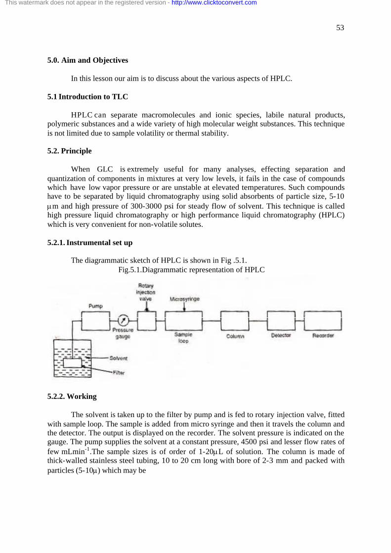
53

5.0. Aim and Objectives In this lesson our aim is to discuss about the various aspects of HPLC. 5.1 Introduction to TLC HPLC can separate macromolecules and ionic species, labile natural products, polymeric substances and a wide variety of high molecular weight substances. This technique is not limited due to sample volatility or thermal stability. 5.2. Principle

When GLC is extremely useful for many analyses, effecting separation and quantization of components in mixtures at very low levels, it fails in the case of compounds which have low vapor pressure or are unstable at elevated temperatures. Such compounds have to be separated by liquid chromatography using solid absorbents of particle size, 5-10 mm and high pressure of 300-3000 psi for steady flow of solvent. This technique is called high pressure liquid chromatography or high performance liquid chromatography (HPLC) which is very convenient for non-volatile solutes. 5.2.1. Instrumental set up

The diagrammatic sketch of HPLC is shown in Fig .5.1. Fig.5.1.Diagrammatic representation of HPLC

5.2.2. Working

The solvent is taken up to the filter by pump and is fed to rotary injection valve, fitted with sample loop. The sample is added from micro syringe and then it travels the column and the detector. The output is displayed on the recorder. The solvent pressure is indicated on the gauge. The pump supplies the solvent at a constant pressure, 4500 psi and lesser flow rates of few mLmin-1.The sample sizes is of order of 1-20mL of solution. The column is made of thick-walled stainless steel tubing, 10 to 20 cm long with bore of 2-3 mm and packed with particles (5-10m) which may be



54

a. Polar solids (Al2O3 Silica gel) for use with low-polarity solvents b. Bonded Phase packing (silica gel to which long-chain alkyl groups are bonded

(C8 or C18 ) by reaction of an alkyl chlorosilane with SiO2) which are suitable for use with polar solvents such as aqueous ethanol.

c. Ion exchange resins, useful for the separation of amino acids o r inorganic anions.

In G.L.C, it is the stationary phase and the temperature is key factors affecting the

separation of mixtures. But in HPLC, it is the choice of solvent or solvent mixture which determines the efficiency of separations.

5.2.3. Detector

The detectors used in HPLC measure the property of the solution or solutes. The solution property may be either refractive index or conductance where the solute properties may be measured by spectrophotometer or spectrofluorimeter. 5.3. Application of HPLC 5.3.1. A chromatogram of water pollutants

A pre concentration step where the sample is subjected to solvent extraction to reduce the volume is often required before the analysis with HPLC . This is particularly necessary for the analysis of Poly aromatic hydrocarbons in water or pesticide residue in food.

Alternatively, water samples may be absorbed on a solid absorbent (C8 or C18 bonded

silica gel) followed by absorption in a solvent which could be directly fed into an HPLC column. Table: 5.1. Some of the HPLC separations are listed below

Compounds Column Solvent Detector Chlorinated hydro carbon, Pesticides

Silica gel n-heptane Refractometer

Caffeine Silica gel CH3OH/NH4OH Spectrophotometer (UV)

Steroids Silica gel CH3Cl / CH4OH Refractometer Polyaromatic hydrocarbons Silica gel n-heptane Fluorimeter


1. Could you compare the efficiency of HPLC with GLC?

………………………………………………………………………………………………… ………………………………………………………………………………………………… ………………………………………………………………………………………………… ………………………………………………………………………………………………… …………………………………………………………………………………………………



55

Aim and Objectives

This lesson deals with the instrumentation and application of Thin layer

chromatography.

5.5. Introduction Thin layer chromatography was first discovered by Izmailov and Shraiber in 1938.

Further Stahl (1958) perfected the method and developed equipment and standardized adsorbents for the preparation of uniform layers on glass plates. And this technique, chromatography using thin layers of an adsorbent held on a glass plate or other supporting medium is called as thin layer chromatography.

5.6. Experimental Setup 5.6.1. Preparation of thin layers on plates

Coating of glass plates with adsorbent layer is made by spreading, pouring, spraying or dipping. The adsorbent layer may be solid or loose. For solid layers, a uniform layer of adsorbent material could be applied to a lean glass plate with an applicator. The applicator used for the preparation of 0.25 mm layer thickness film is the Stahl’s original applicator. Sometimes a binder such as calcium sulphate is added to the adsorbent in small quantities before coating. Loose layers may be prepared by dipping the plates in the suspension, spraying a thin suspension or pouring of suspension on to the plate.

5.6.2 Application of sample on the chromo plates The application of sample on the chromo plates are similar to those used in paper

chromatography. In T.L.C. 0.1 – 1 % solution of the sample are applied to the plates with the help of capillaries, micropipettes and micro syringes. The sample solution could be applied as single sports in a row along one side of the plate, about 2 cms from the edge.

5.6.3 Choice of adsorbent The commonly used adsorbents in TLC are silica gel, alumina, Kieselguhr and

powdered cellulose. Silica gel is the most widely used adsorbent. It is slightly acidic in nature. Alumina is basic, and Kieselguhr is a natural adsorbent.

Layers of about 0.25 mm thick can be prepared by spreading aqueous slurry of the adsorbent with a commercial applicator on glass plates. Thick layers are air dried for about ten minutes and then activated by heating in an oven at 1100 C for 2 hours.

5.6.4 Choice of solvents The choice of solvent depends on the nature of substances to be separated and the

material on which the separation is to be carried out. Polar solvents are preferred, because it results in better separation. And a combination of two solvents too gives better results. Hence the solvent mixture which is highly preferred for its efficiency is n-hexane-diethyl ether acetic acid in the ratio 90:10:1.

5.6.5 Developing chamber The thin layer chromatoplates are usually developed by placing them on edges in the

jar containing a 0.5 – 10 cm layer of the solvent. The jar is then covered with an air tight lid. After the developing solvent ascends for about 10-12 cm above the origin, the plate is taken out of the jar.



56

5.6.6 Detecting reagents. Detecting reagents used in paper chromatography may be used in T.L.C. also. Iodine

dissolved in an organic solvent could be sprayed to deduct many components. Sulphuric acid also forms complex which are colored and visible in day and all light.

5.6.7 Development and detection The various development techniques available include ascending development,

horizontal development, multiple development, stepwise development, gradient development, continuous development and two dimensional development. Normally ascending development is commonly used. During ascending development the sample is spotted at one end of the plate and then developed by ascending technique. The plates are usually placed vertically in a container saturated with developer vapor and solvent.

5.7. General Procedure A plate made of glass is coated with a loose powder or with slurry of an adsorbent.

This slurry adheres to the surface of the glass plate as a thin layer. The unknown substance and reference materials are dissolved in water or an organic solvent and the solution is applied in a row of spot 1-2 cm from the edge of the plate, with micropipette o r micro syringe. The chromatoplate is placed in a jar containing the solvent for development and the jar is lined inside with filter paper which acts as a wick and saturates the atmosphere of the jar with the vapors of the solvent. The jar is covered with an air tight lid. As the solvent ascends by capillary action, the sample gets resolved into fractions. When the solvent front has migrated about 75% of the plate, the plate is then dried and sprayed with to iodine vapor. The position of the fractions would be indicated as brown spots.

5.8. Types of TLC Adsorption TLC: Scientist Kucharezyk (1963) has used adsorption TLC for the

fractionation and analysis of petroleum products. Further it has been used for analysis of waxes and fats, for analysis of essential oils, analysis of carotenoids, steroids, fat soluble vitamins and certain alkaloids by different scientists.

Ion exchange TLC: This type of TLC has been used for the separation of ionic compounds from non ionic compounds. It has been used for the fractionation of short chain carboxylic acids, sugars, amino acids, nucleotides and detergents.

The other types of TLC include the Partition T.L.C. and Reverse phase partition T.L.C.

5.9 Advantages of TLC § The technique helps in the separation of even microgram of the substances. § The separation is very sharp.

It is used to study various biological changes, to study fractionation of large

number compounds, to analyze urine and blood samples.

Self-Check Exercise 2 2. Could you list out the various types of TLC? ………………………………………………………………………………………………… ………………………………………………………………………………………………… ………………………………………………………………………………………………… ………………………………………………………………………………………………… …………………………………………………………………………………………………



57

5.10. Let us sum up. In this lesson we have clearly discussed

· The principle of HPLC

· The working mechanism of HPLC

· The applications of HPLC.

We have also discussed

· The methodology of TLC,

· The steps to be followed

· The advantages

5.11. Lesson end activities · You can prepare a list of natural products, polymers and high molecular weight

substances.

· You can visualize the pipettes, micropipettes and capillary tubes to check the difference in their nature.

5.12. Points for discussion ü Could you narrate the important applications of Thin layer chromatography?

5.13. Check your progress · For the question given above you will surely list various information with respect

to TLC in detail. It is very important that you write the essential information such as : Application of sample on the chromo plates , Choice of adsorbent, Choice of solvents, Developing chamber ,Detecting reagents, Development and detection and also the General Procedure. 5.14 References

1. Scott, R. P. W., ed., Small Bore Liquid Chromatographic Columns: Their Properties and Uses, John Wiley, New York, 1984.

2. Simpson, C.F., ed., Techniques in Liquid Chromatographic Columns: Their Properties and Uses, John Wiley, New York, 1984.

3. Snyder, L.R., AND J.J. KIRKLAND, Introduction to Modern Liquid Chromatography, 2nd ed., Wiley-Interscience, New York, 1979.

4. Yeung, E.S., ed., Detectors for Liquid Chromatography, Wiley-Interscience, New York, 1986.

5. Katz, E., K. Ogan, AND R. P. W. Scott, “LC Column Design,” J. Chromatogr., 289, 65-83 (1984).

6. Willoughby, R.C., AND R.C. browner, “Monodisperse Aerosol Generation Interface for Combining Liquid Chromatography with Mass Spectroscopy,: Anal. Chem., 56, 2626 (1984).

7. Dougles A Skoog and Donald M. West .Principles of Instrumental Analysis – 8. Eiassett. R.C.Denney, G.H. Jeffery, J. Mendham Voges .Text Book of Quantitative

Inorganic Analysis and Elementary Instrumental Analysis 9. Willard, Merril and Dean .Instrumental Methods of Analysis . 10. Chatwal and Anand .Instrumental Methods of Chemical analysis

11. B.K. Sharma .Instrumental Methods of Analysis .



58

UNIT-II Lesson 6. INFORMATION ON ANALYTICAL METHODS. Contents


6.1 Introduction.

6.2 Advantages of analytical methods

6.3 Limitation of analytical methods

6.4 Precision and Accuracy of analytical methods

6.4.1 Sensitivity and detection limits

6.5 Errors

6.5.1 Classification and Minimization of errors

6.6 Let us sum up.


6.8 Points for discussion 6.9 Check your progress

6.10 References 6.0 Aims and Objectives

In the present lesson we will discuss about the accuracy, precision, sensitivity and detection limits. Further we will see about the types of errors and minimization of the same. 6.1 Introduction It is a well known fact that measurement whether it is weight, volume or pH etc., is of only limited accuracy. It is therefore true that the degree of uncertainty will be associated with all the measurements. So it is essential that all the analysis must be repeated to obtain accuracy and the error must be minimized. 6.2 Advantages of Analytical methods

Though the analytical methods could be selected on the basis of the physical property to be measured, they have various advantages. The advantages of analytical methods are as follows:

-High sensitivity could be obtained. -Reliable measurements could be made. -The determination would be very fast. -Even complex samples can be handled easily and accurately. -The quantity of sample needed is small.



59

6.3 Limitations of analytical methods

The limitations of analytical methods are as follows: For analytical techniques continuous calibration is required. The accuracy and the level of sensitivity that could be obtained using the instrument

depend on the nature of the instrument. The cost of the equipment is higher. For various instrumental analyses, specialized training is needed. And for certain instruments space required is higher.


1. What are the advantages of analytical methods? ………………………………………………………………………………………………… ………………………………………………………………………………………………… ………………………………………………………………………………………………… ………………………………………………………………………………………………… ………………………………………………………………………………………………… ………………………………………………………………………………………………… 6.4 Precision and Accuracy of analytical methods.

Precision is a term which could be defined as the degree of agreement between different values obtained under substantially the same experimental conditions. When the precision of the used method is greater, then the standard deviation, S of the values obtained will be smaller. The precision of a particular analytical method could be improved by repeated analysis and also by application of statistical treatment.

Accuracy may be defined as the agreement of a measurement with the known true

value for the quantity being measured. It is also true that the precision is related intimately to the accuracy.

6.4.1 Sensitivity and detection limits.

The sensitivity of the analytical method depends upon the experimental conditions. And the maximum sensitivity which a method could perform is called its detection limit.

The detection limit could be further defined as the maximum concentration of the

substance that could be measured using an instrument and after which the signal just disappears as it is above the limit.

The detection limit of certain instrumental methods has been formulated by F.W.

KARASEK (1972) as follows.



60

Tab.6.1. Detection limits of different analytical methods

Sl.no Methods Detection

limits. 1. UV

Spectrophotometry 10-7

2. IR Spectrophotometry

10-7

3. Gas Chromatography

10-6 to 10-12

4. N.M.R 10-7 5. Mass spectrometry 10-6 to 10-12

6.5 Errors.

Though there are various methods for the analysis of different samples, the potential

source of error exists for all the sampling methods, analysis technique and for the instrumental analysis. Hence it becomes essential to define the magnitude of the error with statistical techniques. In order to get reliable results from the selected analytical method, sources of errors must be identified, eliminated or otherwise minimized.

6.5.1. Classification and minimization of errors.

Errors may be classified as two different errors. They are systematic (determinate) and random (Indeterminate).

The systematic error is otherwise called as the procedural error. This error may be

formed due to improper instrument calibration procedures, impure reagents, and improper operation of the measurement instrument. This error cannot be minimized by just application of statistical methods. These errors could be identified and minimized by modifying the analytical procedure.

The random error is caused due to the measurement technique. This error occurs in

every analysis. The magnitude of the random error is usually small and can be minimized by upgrading the hardware or the software involved. Self-Check Exercise 2

2. Is it possible to minimize the error caused due to the usage of low grade chemicals for

the preparation of reagents? ………………………………………………………………………………………………… ………………………………………………………………………………………………… ………………………………………………………………………………………………… ………………………………………………………………………………………………… ………………………………………………………………………………………………… …………………………………………………………………………………………………



61

6.6. Let us sum up

In this we have studied about the · Accuracy, · Precision, · Errors · Types of errors, · Methods to minimize the errors.


· You can understand the accuracy by using a micropipette to measure 0.1 ml. · Pipette 0.1 ml using ordinary pipette too. · Compare the solution pipetted out.


ü “Any analytical methods would be accompanied by errors.” Substantiate the statement.

ü Explain the terms precision and accuracy.


· For the first question you would have said yes. As there are always chances for errors it has to be accepted that any analytical method will have errors.

Further you can substantiate the chance for getting error as follows: Though there are various methods for the analysis of different samples, the potential source of error exists for all the sampling methods, analysis technique and for the instrumental analysis.

You can then insist the importance of checking the magnitude of error as below: Hence it becomes essential to define the magnitude of the error with statistical techniques. In order to get reliable results from the selected analytical method, sources of errors must be identified, eliminated or otherwise minimized.

It becomes essential to mention about the types of errors also. Errors may be classified as two different errors. They are systematic (determinate) and random (Indeterminate).

The systematic error is otherwise called as the procedural error. This error may be formed due to improper instrument calibration procedures, impure reagents, and improper operation of the measurement instrument. This error cannot be minimized by just application of statistical methods. These errors could be identified and minimized by modifying the analytical procedure.

The random error is caused due to the measurement technique. This error occurs in every analysis. The magnitude of the random error is usually small and can be minimized by upgrading the hardware or the software involved. Thus you can make the concept clear.

· And with respect to the second question, accuracy is a term which is connected with

all analytical procedures. As we have discussed about accuracy in the lesson you can define the term along with the definition of the term Precision too.



62

6.10 References 1. Currie, L., “Sources of Error and the Approach to Accuracy in Analytical Chemistry,”

Chap. 4, Treatise on Analytical Chemistry, 2nd ed., I.K.olthoff and P. Elving, eds., Part I Vol. 1, John Wiley, New York, 1978.

2. Mandel, J . , “Accuracy and Precision: Evaluation and Interpretation of Analytical Results,” Chap. 5. Treatise on Analytical Chemistry, 2nd ed., I. Kolthoff and P. Elving, eds., Part I, Vol. 1, John Wiley, New York, 1978.

3. Meyers, S., Data Analysis for Scientists and Engineers, John Wiley, New York, 1975. 4. Miller, J., AND J. Miller, Statistics for Analytical Chemistry, Halsted, New York, 1984. 5. Dougles A Skoog and Donald M. West .Principles of Instrumental Analysis – 6. Eiassett. R.C.Denney, G.H. Jeffery, J. Mendham Voges .Text Book of Quantitative




63

Lesson 7 BASIC PRINCIPLES OF SPECTROSCOPY. Contents


7.1 Introduction

7.2 Electro magnetic radiation

7.3 Spectroscopy.

7.4 Wave properties and parameters

7.5 Interaction of EMR with matter

7.5.1 Laws of absorption

7.5.2 Optical methods

7.6 Let us sum up.


7.8 Points for discussion 7.9 Check your progress 7.10 References 7.0 Aim and Objectives In this lesson we will discuss about the electromagnetic radiation, its interaction with matter, wave properties, principle of optical methods, principles of spectroscopy. 7.1 Introduction Spectrophotometry is the quantitative study of electromagnetic spectra. Spectrophotometry deals with visible light, near- ultraviolet, and near- infrared. Spectrophotometry involves the use of a spectrophotometer. A spectrophotometer is a photometer (a device for measuring light intensity) that can measure intensity as a function of the color, or more specifically, the wavelength of light. There are many kinds of spectrophotometers. Among the most important distinctions used to classify them are the wavelengths they work with, the measurement techniques they use, how they acquire a spectrum, and the sources of intensity. Other important features of spectrophotometers include the spectral bandwidth and linear range. Perhaps the most common application of spectrophotometers is the measurement of light absorption. Strictly, even the emission half of a luminescence instrument is a kind of spectrophotometer.

There are two major classes of spectrophotometers; single beam and double beam. A double beam spectrophotometer measures the ratio of the light intensity on two different light paths, and a single beam spectrophotometer measures the absolute light intensity. Although ratio measurements are easier, and generally stable, single beam instruments have advantages; for instance, they can have a larger dynamic range.


http://en.wikipedia.org/wiki/Electromagnetic_spectrum

http://en.wikipedia.org/wiki/Visible_spectrum

http://en.wikipedia.org/wiki/Ultraviolet

http://en.wikipedia.org/wiki/Infrared

http://en.wikipedia.org/wiki/Photometer


64

7.2 Electromagnetic radiation

EMR may be considered as an electromagnetic wave traveling at the speed of light. The radiation consists of discrete particles (quanta) of energy, known as photons. The term radiation includes electromagnetic radiations ranging from the electric waves of low frequency through UV rays, visible spectrum, IR rays to the high frequency X-rays and γ-rays. It is also true that EMR requires no supporting medium for its transmission and can pass through vacuum.

7.3 Spectroscopy

It could be defined as the branch of science which deals with the study of interaction of EMR with matter. Spectroscopy is one of the most powerful tools available for the study of wide range of samples. The study of spectroscopy can be carried out under atomic spectroscopy and molecular spectroscopy.

7.4 Wave Properties and Parameters

EMR may be regarded as an alternating electrical field in space associated with the

electric field. At right angles to it, there exists magnetic field. It is possible to represent the wave properties for the radiation by electrical and magnetic vectors.

Fig.7.1. A portion of an electromagnetic wave traveling in the x direction, the

electrical component E & the magnetic component, M

Wave parameters: The EMR can be described in a number of properties. These are: Wavelength: it is the distance from crest units used for expression wave length includes nano-meter, millimicron, micrometer and Angstrom. 1µm = 10-6m 1mµ = 10-9m 1µm = 10-9m Frequency: it is defined as the number of waves per second.

Speed of light in cm/sec Frequency =

M

H



65

Wave length in cm γ = C / λ

The unit for frequency is cycles per second (H), Hertz.

Wave number (γ): The number of waves per unit length is known as wave number and is expressed as the reciprocal of wave length thus,

γ = 1 / λ The unit for wave number is cm-1 The wavelength frequency and wave number are related as follows:

(1 / λ) = γ = γ / C Power (P): Energy per unit time is called power .The power is also called as intensity. Energy constant (E): The energy constant of a photon is directly proportional to the frequency.

\E =h γ

h = Planck’s constant (6.627X10-27 erg/sec) as γ = C / λ

Hence as the Energy increases, the wavelength decrease, and the frequency is directly proportional to energy. 7.5 Interaction of EMR with matter

The interaction of radiation and matter takes place throughout the entire electromagnetic spectrum. The electromagnetic spectrum extends from cosmic rays to radio waves. Within these extremes are the rays such as gamma rays, x-rays, far, middle and near ultraviolet rays, the visible spectrum, IR rays and microwaves.

These radiations when they react with matter, the effects produced will vary in its

nature. In the IR region, the sorption of radiation causes changes in rotational and rotational-vibrational energy states. In the visible and UV region the absorption of radiation, can change the energy of the valence electrons. X rays cause the ejection of inner electrons from matter and the gamma rays on absorption of radiation cause changes in the nucleus.

When EMR passes from Vacuum to the surface of a portion of matter, the radiation

may be absorbed, transmitted, reflected or scattered. ABSORPTION: is a process in which certain frequencies may be selectively removed

when a beam of radiation is allowed to pass through a transparent layer of a solid, liquid or gas.

When an atom or molecule absorbs energy, they will move to higher energy state or

excited state. Excited atoms or molecules are short lived and tend to come back to their ground state after 10-8 sec, with emission of certain amount of energy.

When the emission of light is instantaneous, it is called fluorescence but when there is

some time lag it is called phosphorescence. When the absorbed energy is stored by the atom or molecule and used in producing some chemical reaction, it results in photo-chemical reaction.

In emission, the electron comes down from E* to Eo with the emission of photon and

energy.



66

Fig.7.2. A simple energy level diagram

Eo refers to the lower energy level

E* refers to the higher energy level Transition between electron levels is found in UV and visible regions. Thus

absorption spectra are readily measured in spectral region and are of importance in analytical studies. Self-Check Exercise 1

1. What is wave number? Explain. ………………………………………………………………………………………………….. ………………………………………………………………………………………………….. ………………………………………………………………………………………………….. ………………………………………………………………………………………………….. …………………………………………………………………………………………………..

Laws of Absorption There are two fundamental laws related to the absorption of monochromatic radiant energy by homogenous transparent systems. 1. Lambert law or Bouguer’s law When monochromatic light passes through a transparent medium, layers of equal thickness of that homogenous absorbing medium absorb equal proportions of incident radiation. 2. Beer’s law

The fraction of the monochromatic radiant energy absorbed on passing through a solution is directly proportional to the concentration of the absorbent. From I law dp= -k1 Po dbà1 where b = thickness; Po= radiant power of the beam From II law dp= k2 P1 dcà2 On combining 1 & 2

E*

Emission Absorption

Eo



67

Log P0 / P = abc = A (absorbance) Diffraction of Radiation When a beam of EMR pass through a sharp edge or a narrow opening t he bendening of radiation occurs called diffraction. Dispersion of Radiation The dispersion of radiation through out the electromagnetic spectrum is related to the degree to which radiation is absorbed. They may be normal or anomalous dispersion. Refraction of Radiation. When a beam of radiation is allowed to pass from one medium to another having a change in density, an abrupt change in the direction of the beam is seen, it is called refraction. It is due to the differences in the velocity of radiation in two medias. Reflection of Radiation This phenomenon occurs when a beam of radiation is allowed to pass through media of different refractive indices. Scattering of Radiation When a turbid solution is brought in the light path of a photometer, less radiant energy reaches the photo detector due to scattering of light. Self-Check Exercise 2

a. What are crests and troughs? Explain. ………………………………………………………………………………………………….. ………………………………………………………………………………………………….. ………………………………………………………………………………………………….. ………………………………………………………………………………………………….. ………………………………………………………………………………………………….. 7.5.1 Optical methods

Instruments that measure the transmittance or absorbance of solution contain five basic components.

1. A Stable light source 2. A monochromator 3. Sample containers for sample and solvent 4. A radiation detector 5. A signal indicator

Radiation Source



68

Sources of visible radiation: Tungsten filament lamp. Sources of Ultraviolet radiation: H2 and Deuterium lamps Sources of IR radiation: A coil of nichrome wire can be used as IR source. Wavelength Selection It can be done by

1) The use of filters 2) Dispersion by means of prism or diffraction grating.

Absorption filters consist of colored glass and a interference fitter consists of

transparent CaF2 that occupies the space between two semitransparent metallic films coated on the inside surface of two glass plates. Monochromator:

It is used to separate polychromatic radiation into a suitable monochromatic form. It is a device that resolves radiation into its component wavelength and permits the isolation of any desired portion of the spectrum from the remainder. Such devices may be prisms or gratings. Fig.7.3 Schematic diagram of a Spectrophotometer In a prism monochromator, light administered through an entrance slit is collimated by a lens and then strikes the surface of the prism at an angle. This deflects the beam through an angle depending on the wavelength. The dispersed radiation is then focused on a curved surface containing the slit. Radiation of the desired wavelength may be caused to pass through the exit slit by rotation of the prism and with grating it is by rotating he grating. Sample Containers Cells or cuvettes used are made up of different substances as follows. Quartz and / or fused silica in UV region and glass is used in visible region. For solid samples in IR region, they are either dissolved in liquid paraffin or mixed with alkali halide e.g. KBr.



69

Detectors

The common detection devices are photocells, photo multipliers, photographic plates, thermocouples and photo conductive cells.

Essential characteristics of a detector

1. It should be sensitive to low levels of radiant power. 2. It should respond rapidly to the radiation 3. It should produce an electrical signal that can be amplified.

Two types of Detector

DETECTOR

Heat detectors Photon detectors. E.g. Thermocouple Thermistor

1. Thermocouple: is the most widely used Infra red detector and operates on the basis of heat detection.

2. Bolometer: is a miniature resistance thermometer with a tiny platinum wire as sensing element.

3. Thermistor: is made by sintering together several metallic oxides. 4. Photomultipliers: operate on the principle of photon amplification. A photon striker a

photo cathode gets multiplied y striking a series of anodes resulting in electron multiplication.

5. Photovoltaic cells: in which the radiant energy generates a current at the interface of a semi-conductor and a metal are used for the detection and measurement of radiation in the visible region.

6. Photographic Plate: has an advantage that it integrates radiant energy over a period of time.

Table.7.1. Detectors for EMR

Region Detector Comments Uv region Near I. R I. R

P h o t o e m i s s i v e c e l l Photomultiplier cell Thermocouple Bolometer

Useful in 200nm – 1 mm Used in region 0.8 – 40 mm Used in region 0.8 – 40 mm


3. Define and differentiate reflection, refraction and dispersion of radiation. ………………………………………………………………………………………………… …………………………………………………………………………………………………….……………………………………………………………………………………………… ………………………………………………………………………………………………… ……………………………………………………………………………………………………………………………………………………………………………………………………



70

7.6 Let us sum up

In this lesson we have seen about · Properties of electromagnetic radiation · Its interaction with matter · Basic principles of spectroscopy · Laws of absorption


· Draw the entire sketch of EMR with wavelength. · Understand about UV, IR, far IR rays. · Check the information with a book on chemistry.


ü Describe the source of EMR and add a note on EMR. ü Discuss the laws governing the process of absorption of radiation


· As per the first question in the previous section it is essential to describe about the electromagnetic radiation as we have studied in this lesson. According to want we have learnt, the electromagnetic spectrum extends from cosmic rays to radio waves. Within these extremes are the rays such as gamma rays, x-rays, far, middle and near ultraviolet rays, the visible spectrum, IR rays and microwaves.

Followed by the information on EMR, we can elaborate on its interaction with matter if it is essay question. These radiations when they react with matter, the effects produced will vary in its nature. In the IR region, the sorption of radiation causes changes in rotational and rotational-vibrational energy states. In the visible and UV region the absorption of radiation, can change the energy of the valence electrons. X rays cause the ejection of inner electrons from matter and the gamma rays on absorption of radiation cause changes in the nucleus. When EMR passes from vacuum to the surface of a portion of matter, the radiation may be absorbed, transmitted, reflected or scattered.

· For the second question you will clearly start defining the term absorption followed

by the laws on absorption, that is Lambert’s law and Beer’s law. You will also mention about the equations obtained on the basis of these laws. You will also include the energy level diagram as it will give a clear idea regarding the concept.

7.10 References 1. Bauman, R.P. Absorption Spectroscopy, John Wiley, New York, 1965. 2. Peters, D.G. J.M. Hayes, AND G. M. Hieftje, Chemical Separations and Measurements,

Chap. 18, Saunders, Philadelphia, 1974. 3. Svelto, O., and D.C. Hanna, Principles of Lasers, 2nd ed., Plenum, New York 1982. 4. Thyagarajan, K., AND A. K. Ghatak, Lasers, Theory and Applications, Plenum, New

York, 1981. 5. Dougles A Skoog and Donald M. West .Principles of Instrumental Analysis –



71

6. Eiassett. R.C.Denney, G.H. Jeffery, J. Mendham Voges .Text Book of Quantitative Inorganic Analysis and Elementary Instrumental Analysis

7. Willard, Merril and Dean .Instrumental Methods of Analysis. 8. Chatwal and Anand .Instrumental Methods of Chemical analysis 9. B.K. Sharma .Instrumental Methods of Analysis.



72

Lesson 8. INSTRUMENTATION AND APPLICATION OF ULTRAVIOLET AND VISIBLE SPECTROPHOTOMETERS Contents 8.0. Aim and Objectives

8.1. Introduction


8.2.1. Light Source

8.2.2. Monochromator.

8.2.3 Detector

8.2.4. Working principle

8.3. Types of visible spectrophotometers

8.4. Applications of visible spectrophotometers


8.6 Introduction to UV spectroscopy

8.7 Principle of UV spectrometry

8.8Instrumentation

8.8.1. Light source

8.8.2 Monochromator

8.8.3 Cuvette

8.8.4 Detector

8.9 Special methods in UV spectrophotometric analysis

8.10 Applications of UV spectrophotometer

8.11 Let us sum up




8.15 References



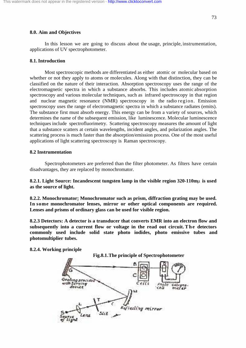
73

8.0. Aim and Objectives In this lesson we are going to discuss about the usage, principle, instrumentation,

applications of UV spectrophotometer. 8.1. Introduction

Most spectroscopic methods are differentiated as either atomic or molecular based on whether or not they apply to atoms or molecules. Along with that distinction, they can be classified on the nature of their interaction. Absorption spectroscopy uses the range of the electromagnetic spectra in which a substance absorbs. This includes atomic absorption spectroscopy and various molecular techniques, such as infrared spectroscopy in that region and nuclear magnetic resonance (NMR) spectroscopy in the radio region. Emission spectroscopy uses the range of electromagnetic spectra in which a substance radiates (emits). The substance first must absorb energy. This energy can be from a variety of sources, which determines the name of the subsequent emission, like luminescence. Molecular luminescence techniques include spectrofluorimetry. Scattering spectroscopy measures the amount of light that a substance scatters at certain wavelengths, incident angles, and polarization angles. The scattering process is much faster than the absorption/emission process. One of the most useful applications of light scattering spectroscopy is Raman spectroscopy. 8.2 Instrumentation Spectrophotometers are preferred than the filter photometer. As filters have certain disadvantages, they are replaced by monochromator. 8.2.1. Light Source: Incandescent tungsten lamp in the visible region 320-110mm is used as the source of light. 8.2.2. Monochromator: Monochromator such as prism, diffraction grating may be used. In some monochromator lenses, mirror or other optical components are required. Lenses and prisms of ordinary glass can be used for visible region. 8.2.3 Detectors: A detector is a transducer that converts EMR into an electron flow and subsequently into a current flow or voltage in the read out circuit. T h e detectors commonly used include solid state photo iodides, photo emissive tubes and photomultiplier tubes. 8.2.4. Working principle Fig.8.1.The principle of Spectrophotometer


http://en.wikipedia.org/wiki/Atomic

http://en.wikipedia.org/wiki/Molecular

http://en.wikipedia.org/wiki/Absorption_spectroscopy

http://en.wikipedia.org/wiki/Atomic_absorption_spectroscopy

http://en.wikipedia.org/wiki/Atomic_absorption_spectroscopy

http://en.wikipedia.org/wiki/Infrared_spectroscopy

http://en.wikipedia.org/wiki/Nuclear_magnetic_resonance_spectroscopy

http://en.wikipedia.org/wiki/Radio_frequency

http://en.wikipedia.org/wiki/Emission_spectroscopy

http://en.wikipedia.org/wiki/Emission_spectroscopy

http://en.wikipedia.org/wiki/Luminescence

http://en.wikipedia.org/wiki/Luminescence

http://en.wikipedia.org/wiki/Spectrofluorimetry

http://en.wikipedia.org/w/index.php?title=Scattering_spectroscopy&action=edit

http://en.wikipedia.org/wiki/Raman_spectroscopy


74

‘S’ is a source of radiation which is a tungsten lamp. Light from the radiation source S is allowed to pass, by means of a lens L, through a narrow slit T and then by means of a mirror m to an optical grating G which divides light into narrow spectral regions corresponding to different wavelengths. The light of a desired wavelength emerging from the grating is allowed to pass through the cuvette B containing the solution under examination. The light further passes to photo electric cell D which is in contact with galvanometer. The intensity of light can be measured with the help of cell D. The cuvette B is now replaced by another cuvette C containing pure solvent and the same light is allowed to pass through it and then to cell D. If I0 = Intensity of light which passes the solution It = Intensity of light which passes through the solvent. Then I0 / It = absorbance.

When log I0 / I t is plotted againstl, maximum absorption will be given by the

maximum in the curves fig. 1. Shows an absorption curve for benzene & it has a maximum absorption around 2550Ao wavelength. That wavelength at which the maximum absorption of light takes place is called as l max.

Fig.8.2. Absorption curve for benzene.

The absorbance obtained is also called as the optical density. The value increases with the increase in the concentration of the solution or the sample. Self-Check Exercise 1

1. What is λ max? Explain. ………………………………………………………………………………………………….. ………………………………………………………………………………………………….. ………………………………………………………………………………………………….. ………………………………………………………………………………………………….. ………………………………………………………………………………………………….. 8.3. Types of visible spectrophotometers.

For the sake of convenience they are divided into 3 groups. 1. Those with glass optics. sensitive from 300-800mm 2. Those with quartz optics sensitive from 200-100mm 3. Those covering the range from 100 mm. 4. They can be 1) Manual or non-recording. 2) Automatic or recording.

Non – Recording types include Cenco sheard backmann, Bausch and Lamb, unicam, etc.



75

Recording types include Perkin Elmer, Backmann co., etc., They employ 1) Single beam or 2) Double beam optical systems.

The simplest and least expensive spectrophotometers are direct reading

spectrophotometers. Applications of visible Spectrophotometers

1. It is used for the analysis of various elements such as a) Al g) Fe m) Salicylic acid b) NH3 h) Mg n) urea c) As i) Mn o) glycine d) Co j) Ni e) Cu k) Ti f) F- l) V

2. They are used for identifying compounds 3. To decide the constituents of compounds 4. To measure the concentration of solutions 5. To study H+ ion concentration. 6. To study the structure of inorganic complexes.


1. Is it possible to measure the concentration of any metal in solution using a spectrophotometer?

………………………………………………………………………………………………… ………………………………………………………………………………………………… ………………………………………………………………………………………………… ………………………………………………………………………………………………… ………………………………………………………………………………………………… 8.5 Aim and Objectives

Our aim is to understand about the principle, methodology and advantages of UV spectrophotometers 8.6. Introduction UV spectroscopy

All atoms absorb in the UV region because these photons are energetic enough to excite outer electrons. If the frequency is high enough, photoionisation takes place. UV spectroscopy is also used in quantifying protein and DNA concentration as well as the ratio of protein to DNA concentration in a solution. The utilization of near ultraviolet absorption spectra as an analytical tool has increased in recent years, due to their efficiency.

8.7 Principle of UV spctrometry

The instrument used in ultraviolet-visible spectroscopy is called a UV/Visible

spectrophotometer. It measures the intensity of light passing through a sample (I), and compares it to the intensity of light before it passes through the sample (Io). The ratio I / Io is called the transmittance, and is usually expressed as a percentage (%T). The absorbance, A, is based on the transmittance: A = - log (%T)


http://en.wikipedia.org/wiki/Photoionisation

http://en.wikipedia.org/wiki/Measuring_instrument

http://en.wikipedia.org/wiki/Absorbance


76

8.8 Instrumentation 8.8.1 Light Source

Both high and low voltage hydrogen lamps give rise to continuous spectrum in the region between 180-375m. A deuterium lamp produces very high radiation intensity than H2 lamp. The basic parts of a spectrophotometer are a light source (often an incandescent bulb for the visible wavelengths, or a deuterium arc lamp in the ultraviolet), a holder for the sample, a diffraction grating o r monochromator to separate the different wavelengths of light, and a detector

8.8.2 Monochromator

They must not have glass optics so prisms or quartz or fused silica must be used as

dispersive device. The performance of spectrophotometers related to the design of the monochromator is evaluated by taking

1. The amount of stray radiant energy and 2. Resolution into condition.

8.8.3 Cuvette

Quartz or fused silica may be used for UV – regions. Two cells may be identical but their absorption characteristics may be different in the UV region. Hence it is necessary to use one cell as reference cell and the other as sample cell always. Samples for UV/Vis Spectrophotometry are most often liquids, although the absorbance of gases and even of solids can also be measured. Samples are typically placed in a transparent cell, known as a cuvette. Cuvette is typically rectangular in shape, commonly with an internal width of 1 cm. (This width becomes the path length, L, in the Beer-Lambert law.) Test tubes can also be used as cuvette in some instruments. The best cuvettes are made of high quality quartz, although glass or plastic cuvettes are common. (Glass and most plastics absorb in the UV, which limits their usefulness to visible wavelengths.) 8.8.4 Detectors

UV spectrophotometers use photo multiplier cells or vacuum photo emissive photo

tubes as detectors. . The detector is typically a photodiode or a CCD. Photodiodes are used with monochromator, which filter the light so that only light of a single wavelength reaches the detector. Diffraction gratings are used with CCDs, which collects light of different wavelengths on different pixels.

8.9 Special methodology in UV spectrometric analysis.

A spectrophotometer can be either single beam o r double beam. In a single beam instrument (such as the Spectronic 20), all of the light passes through the sample cell. Io must be measured by removing the sample. This was the earliest design, but is still in common use in both teaching and industrial labs. In a double-beam instrument, the light is split into two beams before it reaches the sample. One beam is used as the reference; the other beam passes through the sample. Some double-beam instruments have two detectors (photodiodes), and the sample and reference beam are measured at the same time. In other instruments, the two


http://en.wikipedia.org/wiki/Incandescent_bulb

http://en.wikipedia.org/wiki/Deuterium_arc_lamp

http://en.wikipedia.org/wiki/Diffraction_grating

http://en.wikipedia.org/wiki/Monochromator

http://en.wikipedia.org/wiki/Transparency_%28optics%29

http://en.wikipedia.org/wiki/Test_tube

http://en.wikipedia.org/wiki/Quartz

http://en.wikipedia.org/wiki/Photodiode

http://en.wikipedia.org/wiki/Charge-coupled_device

http://en.wikipedia.org/wiki/Spectronic_20

http://en.wikipedia.org/wiki/Spectronic_20


77

beams pass through a beam chopper, which blocks one beam at a time. The detector alternates between measuring the sample beam and the reference beam.

8.10 Applications of Ultra violet Spectroscopy

· It is used for identification of vitamins, sterols, hydrocarbons, enzymes, pharmaceuticals.

· Vitamin A can be assayed by measuring its absorbance at 324mm · It is used to determine inorganic substances e.g. Lead measurement in bone ash. · They are used for identifying compounds · To decide the constituents of compounds · To measure the concentration of solutions · To study H+ ion concentration. · To study the structure of inorganic complexes.

Self-Check Exercise 2 2. What is a monochromator? Explain its function. …………………………………………………………………………………………………. ………………………………………………………………………………………………… …………………………………………………………………………………………………. ………………………………………………………………………………………………… …………………………………………………………………………………………………. ………………………………………………………………………………………………… 8.11 Let us sum up We have discussed about

· The principle of spectrophotometers · Types of the spectrophotometers · Applications of spectrophotometers

In this lesson we have seen about

· Basic principles of UVspectroscopy · Instrumentation of UVspectrophotometer · Applications of UVspectrophotometer


· Visualize the instrument · Understand about the lens, cuvette, slit, monochromator · Under about optical density (or) absorbance


ü Briefly discuss the types and applications of Spectrophotometers. ü Discuss the laws governing the process of absorption of radiation.


http://en.wikipedia.org/wiki/Optical_chopper


78


· As the first question is a direct question you will write about the types of spectrophotometers in detail as you have studied in the lesson. It is essential to give side headings while presenting the information. You will then write about the types and about applications of spectrophotometers.

· For the second question it is necessary to start with the principle of visible

Spectrophotometry. Once you have cited the principle, later narrate the schematic diagram. You will now be in a position to write by yourself about the components & the working principle of the visible spectrophotometer. Finally to end the answer you will have say the procedure for estimating the optical density of the given solution. Using a blank, zero absorbance must be set at the λ max of the solution. Then the absorbance of the solution must be measured. Using the standard graph, the concentration of the substance can be obtained. 8.15 References 1. Bauman, R. P., Absorption Spectroscopy, John Wiley, New York, 1962. 2. Burgess, C., and A. Knowles, eds., Techniques in Visible and Ultraviolet Spectrometry,

Vol. 1, Chapman and Hall, New York 1981. 3. Forbes, W. R., Chap. 1, Interpretive Spectroscopy, S.K. Freeman, ed., Reinhold, New

York 1965. 4. Jaffe, H. H., and M. Orchin, Theory and Applications of Ultraviolet Spectroscopy, John

Wiley, New York 1962. 5. West, W., ed., Chemical Applications of Spectroscopy, Vol. IX, Part 1, 2nd ed., John

Wiley, New York, 1968. 6. Dougles A Skoog and Donald M. West .Principles of Instrumental Analysis – 7. Eiassett. R.C.Denney, G.H. Jeffery, J. Mendham Voges .Text Book of Quantitative





79

Lesson 9 INSTRUMENTATION AND APPLICATIONS OF IR SPECTROSCOPY Contents


9.1 Introduction


9.3 Types of Infrared spectroscopy

9.4 Instrumentation of Infrared spectroscopy

9.4.1 Source of radiation

9.4.2 Monochromator

9.4.3 Cuvette

9.4.4. Detector

9.10 Working principle of IR spectroscopy

9.11 Applications of IR spectroscopy

9.12 Let us sum up.




9.11 References


In this lesson we will see about the principle, working mechanism , types, applications and uses of IR Spectroscopy. 9.1 Introduction

It was first discovered by William Herschel in 1800. Later it was developed by William coblentz. The spectrum of EMR seen in IR region is called IR spectra. They provide valuable information about the basic characteristics of the molecule, nature of atoms, spatial arrangement etc.


Consider a diatomic molecule AB. They have 2 nuclei and electrons. These atoms can exist in a number of energy levels. When excited, energy is absorbed and transition occurs. The absorbed energy may set the whole molecule to rotating or causes the vibration of atoms of A and B within the molecule. These changes can occur due to absorption of IR radiation. These vibration or rotation helps in identifying the functional groups.



80

9.3 Types of Infrared spectroscopy They may be of 2 types.

Single beam IR Absorption instrument 4.3.1 Double beam IR Absorption instrument

9.4 Instrumentation of Infrared spectroscopy 9.4.1 Source Source of IR radiation may be

1) Nernst glowers: are constructed from a fused mixture of oxides of zirconium, yttrium and thorium molded in the form of hollow rods 1 -3 mm in diameter and 2 – 5 cm long. These glowers are fragile.

2) Globar: bar of sintered silicon carbide 6 – 8 mm in diameter and 50 mm long has characteristics intermediate between heated wire coils and the Nernst glower. It is self starting and has an operating temperature near 1300oC

9.4.2 Monochromator

Prism monochromator are most effective in IR radiation. According to wavelength it

should be made up of CaF2, KBr, Nacl. The surface should be smooth. Grating monochromator: They are very popular. They are made of Al and are not

attacked by moisture.

9.4.3 Cuvette: The cuvette is made up of Nacl. 9.4.4. Detector: At the short wave length below 1.2 µm, the preferred detection methods are the same as those used for Visible and Ultraviolet radiation. The detectors used at longer wavelengths can be classified into two groups ie, thermal detectors and photon detectors. 9.5 Working principle of IR spectroscopy

The compounds can be examined in vapor phase, as liquids, in solution and in solid state. In solution: Here the compound is dissolved in chloroform and taken in special cell made of Nacl. In solid state: Accurately 1 mg of solid is ground well with 1 drop of hydrocarbon and used for the analysis. In vapor state: Vapor of the sample is introduced into a special cell made of Nacl. A beam of infrared light is produced and split into two separate beams. One is passed through the sample, the other passed through a reference which is often the substance the sample is dissolved in. The beams are both reflected back towards a detector, however first they pass through a splitter which quickly alternates which of the two beams enters the detector. The two signals are then compared and a printout is obtained. Single beam IR absorption Instrument

Here the radiation passes through the sample and then through the entrance slit to monochromator. The detector measures the amount of radiation absorbed by the sample. Double beam IR absorption Instrument



81

Radiation source

Sample Monochromator Detector

Recorder

Amplifying system

Here the source beam is separated into sample beam and reference beam. The two systems combine and pass along optical system to the detector. An oscillating signal is produced, and the degree of oscillation becomes a measure of I0/It, the absorbance of solution. . Fig.9.1.Schematic diagram of Infra red instrument

Interpretation of IR spectra

Each functional group has a characteristic absorption band at a particular wavelength. Hence the group can be found by comparing with standard reference spectrum.

Peak at l Group 1720 –1740 cm-1 aliphatic aldehyde 1705 -1725 cm-1 Ketones

9.6. Applications of IR Spectroscopy

Infrared spectroscopy is widely used in both research and industry as a simple and reliable technique for measurement, quality control and dynamic measurement.

The instruments are now small, and can be transported, even for use in field trials. With increasing technology in computer filtering and manipulation of the results, samples in solution can now be measured accurately (water produces a broad absorbance across the range of interest, and thus renders the spectra unreadable without this computer treatment).

Some machines will also automatically tell you what substance is being measured from a store of thousands of reference spectra held in storage.

By measuring at a specific frequency over time, changes in the character or quantity of a particular bond can be measured.

This is especially useful in measuring the degree of polymerization in polymer manufacture. Modern research machines can take infrared measurements across the whole range of interest as frequently as 32 times a second. This makes the observations of chemical reactions and processes quicker and more accurate.

Techniques have been developed to assess the quality of tea- leaves using infrared spectroscopy.

Infrared spectroscopy has been highly successful for applications in both organic and inorganic chemistry.

Infrared spectroscopy has also been successfully utilized in the field of semiconductor microelectronics http://en.wikipedia.org/wiki/Infrared_spectroscopy - _note-1#_note-1: for example, infrared spectroscopy can be applied to semiconductors like silicon, gallium arsenide, gallium nitride, zinc selenide, amorphous silicon, silicon nitride, etc.


http://en.wikipedia.org/wiki/Polymer








http://en.wikipedia.org/wiki/Silicon

http://en.wikipedia.org/wiki/Gallium_arsenide

http://en.wikipedia.org/wiki/Gallium_arsenide

http://en.wikipedia.org/wiki/Gallium_nitride

http://en.wikipedia.org/wiki/Zinc_selenide

http://en.wikipedia.org/wiki/Silicon_nitride


82

Self-Check Exercise 1 1. What is the wavelength of Infrared radiation? Is it useful in the spectrophotometric

analysis? …………………………………………………………………………………………………. ……………………………………………………………………………………………….……..…………………………………………………………………………………………….. ………………………………………………………………………………………………… ………………………………………………………………………………………………… ………………………………………………………………………………………………… ………………………………………………………………………………………………… 9.7 Let us sum up In this lesson we have seen about

· Basic principles of IR spectroscopy · Instrumentation of IR spectrophotometer · Working principle of IR spectroscopy · Applications of IR spectrophotometer


· Visit Ayurvedic hospital, Coimbatore or other lab to see IR spectrophotometer.

· Understand to manipulate the functional groups present using the graph obtained for the experiment


ü Describe the working mechanism of IR spectrophotometer ü In what way single beam IR spectrophotometer is different from double beam

IR spectrophotometer.


· When the question is so direct as the first question, you may find it easy to answer. But, it is important to always give an introduction to the technique, principle, types working mechanism, application and also the advantages.

· For the second question, briefly explain the concept of single beam IR spectroscopy and then compare with that of double beam IR spectroscopy. Though the initial information’s remains the same finally give the points clearly to differentiate the single beam, double beam IR spectroscopy.



83

9.11 References 1. Berezkin, V. G., Chemical Methods in Gas Chromatography, Elsevier, New York,

1983. 2. Cowper, C. J., and A. J. Derose, The Analysis of Gases by Gas Chromatography,

Pergamon, New York 1983. 3. Drozd, J., Chemical Derivation in Gas Chromatography, Elsevier, New York, 1981. 4. Grob, R. L., ed., Modern Practice of Gas Chromatography, 2nd ed., John Wiley, New

York, 1977. 5. Grob, R.L., and M. Kaiser, Environmental Problem Solving Using Gas and Liquid

Chromatography, Elsevier, New York 1982. 6. Message, G. M., Practical Aspects of Gas Chromatography/Mass Spectrometry, John

Wiley, New York, 1984. 7. Dougles A Skoog and Donald M. West .Principles of Instrumental Analysis – 8. Eiassett. R.C.Denney, G.H. Jeffery, J. Mendham Voges .Text Book of Quantitative

Inorganic Analysis and Elementary Instrumental Analysis 9. Willard, Merril and Dean .Instrumental Methods of Analysis.

10. Chatwal and Anand .Instrumental Methods of Chemical analysis 11. B.K. Sharma .Instrumental Methods of Analysis.



84

Lesson 10 INSTRUMENTATION AND APPLICATION OF NUCLEAR MAGNETIC RESONANCE SPECTROSCOPY Contents


10.1. Introduction

10.2. Quantam Description of NMR


10.3.1. Sample Holder

10.3.2. Magnet


10.3.4. Radio Frequency Receiver

10.3.5. Read out System

10.4. Application

10.4.1. Structural Diagnosis by NMR

10.4.2. Quantitative Analysis

10.5. Let Us Sum Up




10.9 References


This lesion deals with the different aspects of Nuclear magnetic resonance spectroscopy. The application of NMR has also been discussed. 10.1. Introduction

NMR is one of the branches of spectroscopy in which the radio frequency waves

induce transitions between magnetic energy levels of nuclei of a molecule. The magnetic energy levels are formed by placing the nuclei in a magnetic field. Without the application of magnetic field, the spin states of nuclei are not different & the energy level transitions do not occur on application of magnetic field, transition between energy levels takes place.



85

10.2 Quantum description of NMR The elementary particles, neutrons and protons of nucleus possess spin quantam

number, +½ & -½. The magnetic quantam number (m) takes the value of t l to –l. Quantam mechanics tells us that a nucleus of spin & will have 2l + 1 possible orientations. A nucleus with spin ½ will have 2 possible orientations. In the absence of external magnetic field these orientations are of equal energy. If magnetic field is applied then the energy levels split. Each level is given by magnetic quantam number m.

Fig .10.1. Energy levels for a nucleus with a spin quantam number, ½ system (NMR) M = - (1/2) No Field M = + (1/2) Field Ho Applied Such nuclei could be excited to higher level with EMR, when the nucleus gets a

positive charge and starts spinning, a small magnetic field is generated so the nucleus possess magnetic moment, m.

m = g x spin angular momentum g = gyro magnetic ratio. When a nucleus is placed in a system where it absorbs energy, it becomes excited.

When it loses energy it returns to normal state. This process gets repeated. This process of getting excited and unexcited is called a state of resonance. In order to determine the resonance frequency, the energy absorbed by nuclei is measured by varying the strength of magnetic field Ho. The energy absorbed in this process produces a signal at the detector. This signal is further amplified and recorded as a band in the NMR spectrum.


A high resolution NMR spectrometer contains a complex collection of electron equipments.

Fig.10. 2. Schematic diagram of NMR spectrometer. Magnet Sweep Coils

ENERGY

Detector & Amplifier

Recorder

Sweep Generator

Transmitter RF Receiver



86

10.3.1. Sample holder

The sample holders generally used are glass tubes, which are 7.5. Cms long and has 0.3 cms diameter. They must be chemically inert, durable and transparent to radio frequency radiation.

10.3.2. Magnet

A NMR necessarily possesses an electromagnet or permanent magnet. The strength and direction of the magnet should not change from point to point. The strength must be about 20,000 gauss. So the magnet selected for NMR must maintain constant magnetic field, strength and maximum strength must be got. Permanent and conventional electro magnets are used in NMR spectrometers operating up to 100 MHz. Super conducting magnets suits for instrument operating at 230 MHz.


For obtaining a signal the nucleus must undergo resonance. In order to make the nucleus resonate, the precession frequency of the nucleus should become equal to the frequency of the applied radio frequency field Ho, is kept constant, the precession frequency is fixed. In that case in order to bring resonance, the frequency of radio frequency field should be changed so that it becomes equal to the resonance frequency.

If the radio frequency radiation is kept constant, the resonance frequency of the nucleus must be changed by varying the strength of the magnetic field, Ho. This Sweep method is called field sweep method.

Generally this field sweep method is regarded as better because its practicality is good when compared with the other method.

The variation in the strength of the magnetic field is obtained by fixing a pair of Helm halt coil in the pole faces of the main magnet. 10.3.4. Radio frequency receiver

The sample gets magnetized in the presence of magnetic field. When the radio

frequency radiation is passed through such sample, absorption and dispersion occurs. Fig.10. 3. Absorption signal Fig.10. 4. Dispersion signals

Fig 10.3 and Fig 10.4 explain the line shapes associated with adsorption and dispersion. With the line diagrams the resonance frequency could be determined.

The detector separates absorption signal from dispersion signal. The methods of detection are as follows.



87

The first method is radio frequency bridge method and the second method is nuclear induction method. Normally the operator could select the phase of the signal in order to select either the absorption signal or desorption signal.

10.3.5. Readout System

The absorption signal received from radio frequency receiver is amplified and is fed to a chart recorder.


1. Describe the sample holder of a NMR spectrometer. ………………………………………………………………………………………………….. ………………………………………………………………………………………………….. ………………………………………………………………………………………………….. ………………………………………………………………………………………………….. …………………………………………………………………………………………………..

10.4. Application of NMR

The primary application of NMR is in the field of structural determination of various compounds.

10.4.1. Structural diagnosis and determination of NMR

The diagnosis of the structure of the compound is possible with the following information.

The number of main NMR signals would be equal to the protons in the unknown compound.

From the area of the peaks we could understand about the number of hydrogen nuclei present in each group.

NMR spectroscopy has helped to reveal the structure of SOF4, ClF4, H F 2,, polyethylene etc. it is used to study the hydrogen bonding in metal chelates and in organic compounds.

10.4.2. Quantitative analysis

NMR spectroscopy helps to reveal the molar ratio of the components in a mixture. With the resolved band obtained for one of the component in a mixture, the concentration of the component in the mixture could be understood.

For E.g. A mixture containing equal quantities of aldehyde, hydroxyl and aromatic methyl groups, if subjected to NMR spectroscopy analysis, the spectrum obtained will have three peals as shown in Fig. 10.5.

Figure10. 5 Analysis of NMR spectrum.



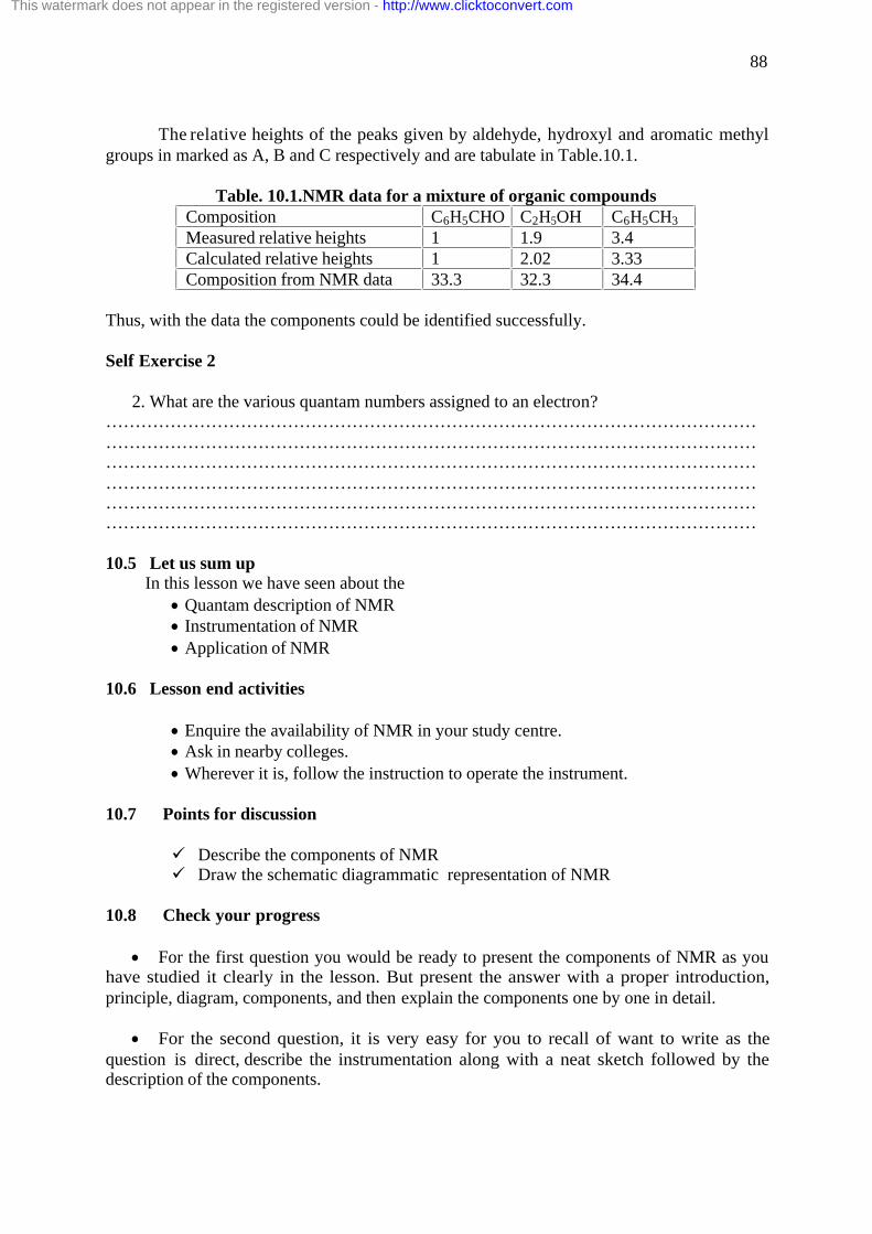
88

The relative heights of the peaks given by aldehyde, hydroxyl and aromatic methyl

groups in marked as A, B and C respectively and are tabulate in Table.10.1.

Table. 10.1.NMR data for a mixture of organic compounds Composition C6H5CHO C2H5OH C6H5CH3

Measured relative heights 1 1.9 3.4 Calculated relative heights 1 2.02 3.33 Composition from NMR data 33.3 32.3 34.4

Thus, with the data the components could be identified successfully. Self Exercise 2

2. What are the various quantam numbers assigned to an electron? ………………………………………………………………………………………………… ………………………………………………………………………………………………… ………………………………………………………………………………………………… ………………………………………………………………………………………………… ………………………………………………………………………………………………… ………………………………………………………………………………………………… 10.5 Let us sum up

In this lesson we have seen about the · Quantam description of NMR · Instrumentation of NMR · Application of NMR


· Enquire the availability of NMR in your study centre. · Ask in nearby colleges. · Wherever it is, follow the instruction to operate the instrument.


ü Describe the components of NMR ü Draw the schematic diagrammatic representation of NMR


· For the first question you would be ready to present the components of NMR as you have studied it clearly in the lesson. But present the answer with a proper introduction, principle, diagram, components, and then explain the components one by one in detail.

· For the second question, it is very easy for you to recall of want to write as the question is direct, describe the instrumentation along with a neat sketch followed by the description of the components.



89

10.9 References 1. Budinger, T. F. And P. C. Lauterbur, “Nuclear Magnetic Resonance Technology for

Medical Studies,” Science. 226, 228 (1984) 2. Cox, R. H. and D. E. Leyden, in Treatise on Analytical Chemistry, 2nd ed., P. J. Elving

M. M. Bursey, and I. M. Kolthoff, eds., Part I, Vol. 10, Chap. 1, John Wiley, New York, 1983.

3. Harris, R. K., Nuclear Magnetic Resonance Spectroscopy, John Wiley, New York, 1986.

4. Jackman, L . M . , and F . A . cottom, eds., Dynamic Nuclear Magnetic Resonance Spectroscopy, Academic, New York, 1975.

5. Kasler, F., Quantitative Analysis by NMR Spectroscopy, Academic, New York, 1973. 6. Willliams, D.A.R., AND D.J. MOWTHORPE, Nuclear Magnetic Resonance

Spectroscopy, John Wiley, New York, 1986. 7. Dougles A Skoog and Donald M. West .Principles of Instrumental Analysis – 8. Eiassett. R.C.Denney, G.H. Jeffery, J. Mendham Voges .Text Book of Quantitative

Inorganic Analysis and Elementary Instrumental Analysis 9. Willard, Merril and Dean .Instrumental Methods of Analysis.

10. Chatwal and Anand .Instrumental Methods of Chemical analysis 11. B.K. Sharma .Instrumental Methods of Analysis.



90

UNIT - III

Lesson 11. INSTRUMENTATION AND APPLICATIONS OF FLAME PHOTOMETER Contents

11.0Aims and Objectives

11.1 Introduction

11.2 Components of Flame Photometer

11.2.1 Pressure Regulator

11.2.2 Atomizer

11.2.3 Burner

11.2.4 Optical System

11.2.5 Detector

11.2.6 Recorder

11.3 Working of the Instrument

11.4 Applications

11.5 Let Us Sum Up




11.9 References


This lesson deals with the flame photometer, i t s components, working of the instrument and its application. 11.1 Introduction

Flame photometry is a technique whereby the concentration of a metal in solution may be determined by spraying the solution into the flame and comparing the emission intensity of the sample with a standard solution of metal.

The events which occur with flame photometer are as follows. On the introduction of

the solvent, it ge ts vaporized, leaving solute particles .Further these solute particles are converted into gaseous state . The gaseous molecules dissociate to give neutral atoms or radicals. These neutral atoms are excited by the thermal energy of the flame. The excited atoms emit photons and return to lower energy state. The emitted photons are measured. The emission intensity is correlated with the concentration of the element.



91

E1 and E2 = energy of lower and higher energy levels. E2 – E1 = hγ 1 h = Planck’s constant γ = Frequency of emitted radiation But γ = c / λ 2 c = velocity of light λ = wavelength of emitted radiation. Sub 2 in 1 E2 – E1 = hc/ λ λ= hc / E2 – E1 using which λ can be calculated.

Components of a flame photometer a) Pressure regulator b) Atomizer c) Burner d) Optical system e) Photo sensitive detector f) Instrument for recording the output of detector

11.2.1 Pressure regulator

A 10 lb/in2 pressure regulator for fuel and a 20 lb/in2 pressure regulator for the air supply must be installed in line from gas cylinders to burners. 11.2.2 Atomizers

It is the one which introduces the spray of the solvent into a condensing chamber. The dispersion of a liquid into particles by a rapidly moving gas, liquid stream or by mechanical means is called as the atomization.

11.2.3 Burner

Two common burner which have been used are 1) Total consumption burner: In this burner, the sample solution, fuel and the oxidizing

gas are passed through separate passages and meet at an opening at the base of the flame. Fig.11.1. Total consumption burner



92

2) Premix burner: Here the fuel, mist of sample, oxidant are mixed & then forced into opening.

The flame temperature lies between 1000 and 30000C. It must produce a steady flame. 11.2.4. Optical System

Glass gelatin and interference filters have been used frequently due to their narrow band widths.

11.2.5. Detectors.

Flame photometers employ vacuum photo tubes, photo tubes or photomultiplier cells as detectors.

11.2.6 Recorder

Generally galvanometer is used for measuring the output of the detector. Fig.11.2. Schematic diagram of a flame photometer.


1. What is the function of an atomizer? ………………………………………………………………………………………………….. ………………………………………………………………………………………………….. ………………………………………………………………………………………………….. ………………………………………………………………………………………………….. …………………………………………………………………………………………………..

11.3. Working of the instrument.

The sample solution is sucked by an atomizer and as a fine spray fed spray fed into the flame. The emitted light is collected by a parabolic mirror and a lens and then allowed to pass through a filter. The light of the selected wavelength strikes a detector and the magnitude of the electrical signal is read on a meter.

The flow rate and the ratio of fuel to oxidant are adjusted using pressure regulators

and flow meters.



93

11.4 Applications

1. Used for the determination of Na, K, Ca in water, cement glass, ash, biological and in clinical materials.

2. When flame photometer is coupled with GC it can be used to detect elements such as Na, K, Li, Mg, Ca, Ba.

3. The Na and K contents in glass melt have been determined. 4. The concentration of Na and K in cement samples can be found out.

Self Exercise 2.

2. What are the various uses of the flame photometer with respect to environmental analysis?

-------------------------------------------------------------------------------------------------------------------------------------------------------------------------------------------------------------------------------------------------------------------------------------------------------------------------------------------------------------------------------------------------------------------------------------------------------------------------------------------------------------------------------------------------------------------------------- Let us sum up We have seen about

· The principle of flame photometer · The components of flame photometer · The working principle of flame photometer · Applications of flame photometer

11.6 Lesson end activities · Check the flame colour obtained for sodium, calcium and Potassium · If dirty water is not free from Sodium and Potassium you can use air as standard

11.7 Points for discussion ü How do you detect the amount of Na in the given water sample? ü Discuss the assemblage of various components of flame photometer.

11.8 Check your progress · For the first question it is important to describe the flame photometer with diagram as

follows: Further you have to mention about the standard graph preparation for Na. Then when you inject the sample, the meter reading would be obtained with which, the amount of sodium can be obtained using the standard graph.

· The second question will make you think about the components of flame photometer. For which you can understand that you have to first state the principle of the instrument, followed by the description of the instrument as shown in the lesson. Further the components must be mentioned with their usage and importance in detail.



94

11.9 References 1. Alkemade, C., et al., Metal Vapors in Flames, Pergamon, New York, 1982. 2. Dean, J., Flame Photometry, McGraw-Hill, New York, 1960. 3. Ottaway, J., and A. Ure, Practical Atomic Absorption Spectroscopy, Pergamon, New

York, 1983. 4. Weltz, b., Atomic Absorption Spectroscopy, Verlag Chemie, New York, 1976. 5. Dougles A Skoog and Donald M. West .Principles of Instrumental Analysis – 6. Eiassett. R.C.Denney, G.H. Jeffery, J. Mendham Voges .Text Book of Quantitative




95

Lesson 12 INSTRUMENTATION AND APPLICATIONS OF ATOMIC ABSORPTION SPECTROPHOTOMETER Contents


12.1. Introduction

12.2. Principle

12.3. Instrument

12.3.1. Radiation Source

12.3.2. Atomizer


12.3.4. Lenses and Slit

12.3.5. Detectors

12.3.6. Read out Device

12.4. Working of the Instrument

12.5. Applications

12.6. Let us Sum Up




12.10 References

12.0. Aims and Objectives This lesson deals with the principle, instrumentation, working and applications of atomic absorption spectrophotometers. 12.1. Introduction.

This technique was introduced for analytical purpose by Walsh and Alleemade, Mihaz (1956) under the designation Atomic absorption spectroscopy. It is found to be superior to other technique as it can be used to determine 50-60 elements from trace to large quantities. These may include metals and non-metals. 12.2 Principle

The sample is first converted into an atomic vapor and then the absorption of atomic vapor is measured at a selected wavelength characteristic of atoms each element. The amount of light absorbed is determined because the absorption is proportional to the concentration of the element.



96


The apparatus consists of 1) Radiation source 2) Atomizer 3) Monochromator 4) Lenses and slits 5) Detectors

12.3.1. Radiation source

Hollow cathode lamp is widely used. It is a thick walled glass tube with a transparent window at one end. Tungsten wires are sealed into other end of the tube, which acts as anode. Other wire is attached to a hollow metal cylinder which acts as cathode. The tube is filled with helium or argon at 1-2 mm pressure.

Fig.12.1. Radiation source sharmap.187

Cathode Transparent Anode Window

12.3.2. Atomizers

It is the one which introduces the spray into the flame. Atomization refers to the dispersion of a liquid into particles by a rapidly moving gas, liquid stream or by mechanical means. Flame Atomization

The burner and a nebulizer help in the atomization of the element. The flame is produced in the burner where the combustion occurs and an atomic vapor of the element to be analyzed is produced. The selection of flame temperature is important for ionization. When it is low, atomization will be incomplete. When it is high, the atoms may be ionized. Graphite furnace atomization

A graphite furnace atomizer is used in graphite furnace atomic absorption spectroscopy. The atomizer may be elongated along its axis to increase the distance between the optical path and the sample deposition point. The elongation of atomizer increases the analytical sensitivity.

Oxidants and fuel

Fuels used are H2, propane, butane, acetylene and natural gas. Widely used is acetylene.

Oxidants used are air enriched with O2, O2 and nitrous oxide.



97

Table.12 .1.Flame and Flame temperature requirement

Flame Temperature Elements Air – Coal gas Air – Propane Air – Acetylene N2O – acetylene

1800 1900 2300 2955

Zn, Cu, Cd, Pb Volatile & noble elements Sn, Ba, Cr etc., Al, V, Tp. Bl, Se etc.


It is important that this instrument must be capable of providing a narrow band width to separate the line chosen for determination from other undesirable lines. Usually used devices are gratings or prisms. 12.3.4. Lenses and slits They are used for the isolation of required spectral line from the total spectrum. 12.3.5. Detectors

Photo multipliers are used as detectors. In some instruments two filters and two detectors are used to compensate the fluctuations in the output of source. The output of photomultiplier is taken to amplifier which helps in source modification. 12.3.6. Read out device

A chart recorder is used as a read out device. Figure.12.2.Schematic diagrammatic representation of Atomic absorption

Spectrophotometer Lens Self-Check Exercise 1

1.What are the fuels used for atomization? ………………………………………………………………………………………………….. ………………………………………………………………………………………………….. ………………………………………………………………………………………………….. ………………………………………………………………………………………………….. ………………………………………………………………………………………………….. 12.4. Working of the instrument

A blank solution is sprayed into the flame and the meter is adjusted for zero

absorbance or 100% transmittance. Now the solution under investigation is sprayed, the atoms in excited state absorbs certain part of light resulting in decrease in transmitted light or increase in absorbed light falling on photomultiplier. This gives a deflection in the meter needle, with the help of standard graph, the concentration of a particular element in the sample can be found out.

Hollow Cathode

Lamp

Flame Nebulizer

Unit

Monochro

mator

Detector and

Readout



98

Fig.12. 3. Standard Graph

0

0.2

0.4

0.6

0.8

1

1.2

1.4

2 4 6 8 10 12

Concentration of Copper (PPM)

Absorb

ance

Interferences

Though atomic absorption spectrophotometers are free from spectral interferences,

they are prone to chemical interferences as discussed below. Chemical interferences

Normally in AAS, chemical interferences could occur, due to the nature of the ions involved. For e.g., the phosphate ions interfere with the determination of calcium and magnesium. The reason is the formation of phosphates of calcium and magnesium, which prevents the easy breakage of Ca and Mg- ions into the flame. This interference could be reduced by the addition of salt of lanthanum or thorium. These salts will form a bond with phosphate ions. Therefore the calcium and magnesium ions can be determined easily. Ionization interference

Such interference can also occur in AAS along with chemical interferences. Such interference occurs when the free metal atom undergoes ionization as follows:

M M+ + e-

This occurs with alkali metals as they need very low energy for their ionization. If a

deionizer or a radiation buffer is added, then this type of interference may be overcome during in the estimation. 12.5. Applications

1. It can be used to determine about sixty metals 2. It can be used to determine Al, Mg, Cu, Zn, Pb, Ni for e.g. many other metals too. 3. Na & K in biological fluids have been determined. 4. Willis has determined Ca & Zn in urine samples of industrial workers. 5. Fe in blood samples can also be found out.



99

6. Council of British Archeology (1964) has used AAS to analyze polluted samples. Lead contamination by automobiles can be found out.

7. In agriculture, soil extracts, plant materials and fertilizers have been analyzed for the determination of Ca, Cu, Fe, K, Mg, Mn, Mo, Na, Sr, Zn.

8. Oils such as crude oil, lubricating oil and feed stocks can be analyzed f o r determination of metals.

9. Impurities in petrol and refined oils can be determined. 10. Electroplating effluents have been analyzed for Cd, Cu, Fe, NP & Zn.

Self Exercise 2.

2. What are the various uses of the atomic absorption spectrophotometer with respect to environmental analysis?

---------------------------------------------------------------------------------------------------------------------------------------------------------------------------------------------------------------------------------------------------------------------------------------------------------------------------------------------------------------------------------------------------------------------------------------------------------------------------------------------------------------------------------------------------------------------------------------------------------------------------------------------------------------------------------------------------------------------------------------------------------------------------------------------------------------- 12.6 Let us sum up We have seen about

· The principle of atomic absorption spectrophotometer · The components of atomic absorption spectrophotometer · The working principle of atomic absorption spectrophotometer · Applications of atomic absorption spectrophotometer


· Visit TNAU Lab to see the AAS · Check the quantity of sample injected for analysis

12.8 Points for discussion ü Describe the method to be adopted to analyze micro quantities of Mercury

accumulated in the greens sampled from contaminated lake. ü Is it possible to analyze the dyes accumulator in fish samples?

12.9 Check your progress · Now you will be in a position to understand and present that for all micro quantity

analysis, the instrument to be preferred is atomic absorption spectrophotometer. You first mention about the choice of instrument. Later you will mention about the principle, components and working mechanism of the instrument. For any biological samples, since triple acid digestion is a must, the greens must be digested and the filtrate must be subjected for the analysis of mercury. Each metal could be analyzed using different methodology.



100

· As you have discussed for the first question it is possible to measure the chromium accumulated in fish tissue samples. A mention must be made that the tissue must be subjected to acid digestion, following which the sample can be fed into the instrument to find out the amount of chromium accumulated in the sample. 12.10 References

1. Alkemade, C., et al., Metal Vapors in Flames, Pergamon, New York, 1982. 2. Dean, J., Flame Photometry, McGraw-Hill, New York, 1960. 3. Ottaway, J., and A. Ure, Practical Atomic Absorption Spectroscopy, Pergamon, New

York, 1983. 4. Weltz, b., Atomic Absorption Spectroscopy, Verlag Chemie, New York, 1976. 5. Dougles A Skoog and Donald M. West .Principles of Instrumental Analysis – 6. Eiassett. R.C.Denney, G.H. Jeffery, J. Mendham Voges .Text Book of Quantitative

Inorganic Analysis and Elementary Instrumental Analysis 7. Willard, Merril and Dean .Instrumental Methods of Analysis . 8. Chatwal and Anand .Instrumental Methods of Chemical analysis 9. B.K. Sharma .Instrumental Methods of Analysis .



101

Lesson 13 INSTRUMENTATION AND APPLICATIONS OF ATOMIC

EMISSION SPECTROPHOTOMETER

Contents 13.0. Aims and objectives

13.1. Introduction

13.2. Types of spectra

13.3 Types of emission spectra


13.4.1. Excitation source

13.4.2. Electrodes

13.4.3. Sample handling


13.4.5. Read out device

13.5. Working of simple prism spectrometer

13.6. Applications of Emission Spectroscopy

a) Comparison sample method

b) Internal standard method

13.7. Let us sum up




13.11 References

13.0. Aim and objectives This lesson deals with the atomic emission spectroscopy, types of emission spectra, Instrumentation, working and its applications . 13.1. Introduction

In atomic emission spectroscopy, a sample is excited by absorbing thermal or electric energy and the radiation emitted by the excited sample is studied for qualitative and quantitative analysis. Emission spectroscopy is regarded as the most reliable method for elemental quantitative.



102

13.2. Types of spectra Emission Spectra: Imagine a substance is heated to a high temperature by thermal or

electric method, and then light is emitted. The light is allowed to pass through a prism or a grating. Further the light is examined with a spectroscope; the spectrum obtained is called as emission spectra.

13.3. Types of Emission spectra

Emission spectra are of three types. Continuous spectra-such spectra depends on the temperature and not on the chemical composition. For eg. Ion and carbon emit continuous spectra when the solids are heated until they glow. Continuous spectra are characterized by uninterrupted emission of light. And sharp lines or discrete bands are absent. But such spectra can not be used for spectro chemical analysis.

Band Spectra: This type of spectra is given out by excited molecules. It is also called

molecular spectrum. In band spectrum the group of lines appears so close together so that they appear as continuous spectra.

Line spectra: A line spectrum consists of discrete irregularly spaced lines. This type of

spectrum is obtained when the light emitting substance is in atomic state. Therefore, it is called atomic spectrum. Line spectrum depends on the type of atom. So it is the predominant type in emission spectroscopy.

The line spectrum is explained on the basis of Bohr’s theory. When an atom is in

ground state, the electrons are present in lowest energy levels. On excitation of the atom by electric or thermal methods, the electrons move from inner orbital to outer orbital. The excited electrons emit energy in the form of discrete special lines. This concept forms the basis of emission spectroscopy.


1. What do you mean by monochromator? ………………………………………………………………………………………………….. ………………………………………………………………………………………………….. ………………………………………………………………………………………………….. ………………………………………………………………………………………………….. …………………………………………………………………………………………………..


The various individual components of the equipment are as follows:

13.4.1. Excitation sources: The excitation sources may be any one of the following.

Flame: Flame is used for those molecules which require low temperature for excitation and dissociation into atoms. It is an inexpensive, stable and reproducible source of excitation.



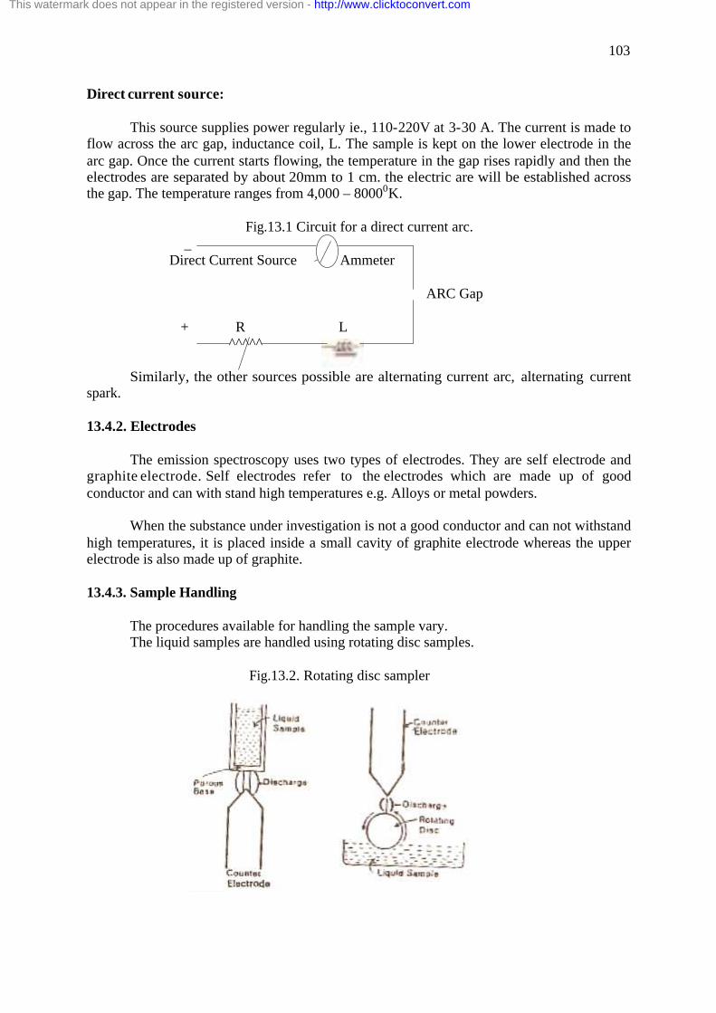
103

Direct current source: This source supplies power regularly ie., 110-220V at 3-30 A. The current is made to

flow across the arc gap, inductance coil, L. The sample is kept on the lower electrode in the arc gap. Once the current starts flowing, the temperature in the gap rises rapidly and then the electrodes are separated by about 20mm to 1 cm. the electric are will be established across the gap. The temperature ranges from 4,000 – 80000K.

Fig.13.1 Circuit for a direct current arc.

_ Direct Current Source Ammeter ARC Gap

+ R L ^^^^^ Similarly, the other sources possible are alternating current arc, alternating current

spark.

13.4.2. Electrodes

The emission spectroscopy uses two types of electrodes. They are self electrode and graphite electrode. Self electrodes refer to the electrodes which are made up of good conductor and can with stand high temperatures e.g. Alloys or metal powders.

When the substance under investigation is not a good conductor and can not withstand

high temperatures, it is placed inside a small cavity of graphite electrode whereas the upper electrode is also made up of graphite.

13.4.3. Sample Handling

The procedures available for handling the sample vary. The liquid samples are handled using rotating disc samples. Fig.13.2. Rotating disc sampler



104

The solid samples are handled in different ways depending on their nature. When the sample has good conductance and can withstand high temperatures, it can

be used as such. When the sample is not a good conductor then it is powdered and mixed with graphite and placed in the lower graphite electrode.

When the sample is loaded, it is placed in the circuit when the electrical discharge

occurs from the top surface of the electrode, the sample is vaporized and the spectrographic emission takes place.


In emission spectroscopy both prism and grating monochromator are used. The

function of the monochromator is to separate the various lines of a sample’s emission spectrum.

13.4.5 Detectors

The detectors widely used include photomultipliers and photographic plates. Photographic plates are used for the qualitative analysis and photomultipliers are used for the quantitative analysis. 13.5 Working of Simple prism spectrometer

The optical system of a simple prism spectrometer is show in Fig.3 Fig.13.3.Working of simple prism spectrometer It consists of an excitation source, which emits light, this light travels through the lens

and further through slit and collimator lens. The light thus emitted reaches dispersing prism, and finally reaches the eyepiece. In the absence of eyepiece a camera lens followed by photographic plate is used.

Generally the prism is made of quarts or fused silica. Other prisms available for use

includes cornu prism, Littrow prism. Self-Check Exercise 2

2. What type of detectors are used for the qualitative analysis of samples? ………………………………………………………………………………………………….. ………………………………………………………………………………………………….. ………………………………………………………………………………………………….. …………………………………………………………………………………………………..



105

…………………………………………………………………………………………………..

13.6. Applications of Emission Spectroscopy We will see about the methods used in quantitative spectrographic analysis.

a) Comparison sample method In this method, the spectra obtained the unknown sample is compared with the

standards; it is possible when the spectra are photographed on the same plate under the same set of conditions. Visual or photometric comparison of blackening may be used.

b) Internal standard method

An internal standard along with the sample is existed in the electrical discharge. The both sample and internal standard emit spectral lines. These are photographed on a photographic plate. Further the intensity of both the emission lines is measured.

Using a set of standard samples a calibration curve is prepared. Using the calibration

curve, the quantity of unknown element could be detected. The standard sample used must be pure in its composition.

Emission spectroscopy is used for the analysis of aluminum alloys, copper alloys,

magnesium alloys, zinc alloys, lead alloys and tin alloys. It is also used to control the composition of the molten metals before their processing. Further it is used to detect the presence of trace elements such as vanadium, copper, iron and nickel in the crude oil, emission spectroscopy has been used to detect presence of many elements such as sodium, potassium, zinc, copper, calcium, magnesium, nickel and iron in tissues of animals and men and in Plants and soils. Even the presence of calcium, copper and zinc could be detected in the blood samples, zinc in pancreas tissue.

Self Exercise 3.

3. What are the various applications of the atomic emission spectrophotometer with respect to environmental analysis?

------------------------------------------------------------------------------------------------------------------------------------------------------------------------------------------------------------------------------------------------------------------------------------------------------------------------------------------------------------------------------------------------------------------------------------------------------------------------------------------------------------------------------------------------------------------------------------------------------------------------------------------------------------------------------------------------ 13.7. Let us sum up We have seen about

· The principle of atomic emission spectrophotometer · The components of atomic emission spectrophotometer · The working principle of atomic emission spectrophotometer · Applications of atomic emission spectrophotometer



106

13.8. Lesson end activities · Try the concept of sample handling by yourself to understand about the concept. · See the functional of detector by altering the samples.

13.9. Points for discussion ü Why is it necessary to excite the sample for its detection? What is the

mechanism behind it. ü Draw the schematic diagram of Atomic emission spectrometer

13.10 Check your progress · To answer the first question you must have studied and understood the principle of the

instrument well. You have to explain the principle as follows. As it is clear that the sample must be excited in order to excite to the excited state, so that detection of the sample becomes possible.

· For the second question, you will be very clear that you need to draw a diagram of the instrument. Yes you are right. But for such question, you must explain the principle of AES, followed by components description and then the diagram of AES. Such presentation will give you high marks

13.11 References 1. Barnes, R., ed., Emission Spectroscopy, Halsted, New York, 1976. 2. Grove, E., ed., Applied Atomic Spectroscopy, Vols. 1 and 2, Plenum, New York, 1978. 3. Schrenk, W., Analytical Atomic Spectroscopy, Plenum, New York, 1975. 4. Walsh, M . , and M. Thompson, A Handbook of Inductively Coupled Plasma

Spectroscopy. Methuen, New York, 1983. 5. Dougles A Skoog and Donald M. West .Principles of Instrumental Analysis – 6. Eiassett. R.C.Denney, G.H. Jeffery, J. Mendham Voges .Text Book of Quantitative




107

Lesson 14 DIRECT READING SPECTROMETER. Contents


14.1 Introduction

14.2 Direct reading double beam spectrophotometer

14.3 Superiority of Direct reading spectrometer.

14.4 Illustration

14.4.1 Condenser

14.4.2 Photo multiplier tube sensitivity

14.5 Advantage of Direct Reading Sensitivity

14.6 Let us sum up.




14.10 References


In this lesson, we will see in detail about the direct reading spectrometers.

14.1. Introduction

Direct reading spectrometers were developed simultaneously and independently at several sites during the mid 1940s. Many leading companies have invented such spectrometers. These instruments do not necessitate the interpretation of photographs of spectral lines; instead the instrument directly displays the concentration of the element. 14.2. Direct reading double beam spectrophotometer. Recording and Non recording spectrophotometers

Almost all recording spectro photometers use the double beam principle. However

commercially available recording double-beam spectrophotometers are direct reading, optical null and Potentiometric null types.

A direct reading double beam spectrophotometer has been devised by Beckman

(model DB-G). In this instrument a vibrating mirror is present in the sample compartment. This mirror permits the monochromatic beam to first pass through the sample solution and then through the reference solution at the rate of 35Hz. Thus, the beam reaching the photomultiplier contains alternating pulses from sample and reference. The signals reaching the photomultiplier tube are differentiated by high-speed magnetic s witch. The magnetic switch directs the reference signal to a regulating circuit where it gets stabilized by constant voltage. It directs the signal from the sample solution to the output meter where its amplitude



108

is directly read on the meter as percent transmittance. This model has a wavelength range from 190-700 mm. Resolution is about 0.2 nm. The interpretation will be made in the instrument directly thereby depicting the composition of the sample. 14.3. Superiority of Direct Reading Spectrometers

A spectrograph consists of the following main parts. It starts with a) source of light, which could be sun, the discharge if an electric are, a flame etc. this light is passed through b) a narrow slit-Further the light is permitted through 3) a dispersing device – a prism or a grating which is used to separate spatially the different wavelengths of light. The dispersed right is then focused on recorder or detector.

With the wavelength of light emitted t he element present in the light source could be

analyzed. If metals are analyzed in a sample, it may take some days to analyze using wet chemical methods. But with direct reading spectrometer it takes just minutes. In Direct reading spectrometers the photo-multiplier tubes and associated electronics directly measure the line intensity. Therefore the operators need not interpret photographs of spectral lines; instead the instrument directly displays the concentration of the elements of interest.

Self-Check Exercise 1 1. Explain the advantages of DR spectrometer .………………………………………………………………………………………………….. ………………………………………………………………………………………………….. ………………………………………………………………………………………………….. ………………………………………………………………………………………………….. …………………………………………………………………………………………………..

14.4. Illustration

A company in 1943 was producing large quantities of magnesium alloy for the construction of air plane. Calcium was a critical element in magnesium alloy. The presence of calcium, would not permit the metal to roll properly, if the calcium content is higher the metal would burn when welded. For the analysis of the alloy, wet chemical methods and photo-spectrographic methods were much too slow. In order to work out the problem, in 1944, an instrument was devised. The instrument initially had problem with electrical and optical problem.

14.4.1. Condensers: condensers attached to photo multiplier tubes, stored the charge generated by the tubes thereby electrically encoding information about line intensity. The company replaced the old condenser with a polystyrene dielectric which was successful in direct reading spectro-photometer. 14.4.2. Photo multiplier tube sensitivity The Cathodes which initially received the light in the photo-multiplier tubes turned out to be finicky. When a ground quartz plate was used the cathode has stable sensitivity.

Thus the Direct reading spectrometer was upgraded and analyzed about 4000 samples of magnesium per months.



109

14.5. Advantages of direct reading sensitivity

The time spent for each determination is minimized. Interpretation is also incorporated reducing the time and energy needed for the same. Self Exercise 2.

2. In what way the direct reading spectrometer is superior than wet chemical methods? ------------------------------------------------------------------------------------------------------------------------------------------------------------------------------------------------------------------------------------------------------------------------------------------------------------------------------------------------------------------------------------------------------------------------------------------------------------------------------------------------------------------------------------------------------------------------------------------------------------------------------------------------------------------------------------------------ 14.6. Let us sum up

We have discussed about

· Direct reading spectrophotometer · Instrumentation · Illustration · Advantages of DRS.


· Check the companies of various available spectrophotometers. · Find out the model number of the spectrophotometer present in your lab

14.8 . Points for discussion ü Do you know about any company who have engineered a DR spectro meter ü What is you opinion regarding direct reading spectro meter, compare with normal old

model colorimeter.

14.9 Check your progress · If you have studied the study material you will be in a position to recall the company.

i.e Beckman (model DB-G) mentioned in the lesson, who have designed the Direct reading spectrometer. You would mention the company and further you have to explain the instrument as follows. A direct reading double beam spectrophotometer has been devised by Beckman (model DB-G). In this instrument a vibrating mirror is present in the sample compartment. This mirror permits the monochromatic beam to first pass through the sample solution and then through the reference solution at the rate of 35Hz. Thus, the beam reaching the photomultiplier contains alternating pulses from sample and reference. The signals reaching the photomultiplier tube are differentiated by high-speed magnetic switch. The magnetic switch directs the reference signal to a regulating circuit where it gets stabilized by constant voltage. It directs the signal from the sample solution to the output meter where its amplitude is directly read on the meter as percent transmittance. This model has a wavelength range from 190-700 mm. Resolution is about 0.2 nm. The interpretation will be made in the instrument directly thereby depicting the composition of the sample.

· For this question, who have to mention the advantages of DR spectrometer. Over other types of colorimeters. Give the advantages as given below to highlight the importance



110

of DR spectrometer. The time spent for each determination is minimized. Interpretation is also incorporated reducing the time and energy needed for the same. 14.10. References

1. Dougles A Skoog and Donald M. West .Principles of Instrumental Analysis – 2. Eiassett. R.C.Denney, G.H. Jeffery, J. Mendham Voges .Text Book of Quantitative




111

Lesson 15- INSTRUMENTATION AND APPLICATIONS OF MASS

SPECTROMETER

Contents :


15.1 Introduction

15.2 Instrumentation

15.2.1 Ion source

15.2.1.1 Plasma excitation

15.2.2.2 Laser excitation

15.2.2.3 Flame excitation

15.2.2 Mass analyzer

15.2.3. Detector

15.3 Tandem MS (MS/MS)

15.4 Common Mass Spectrometer Configurations and Techniques

15.5 Other Separation Techniques Combined with Mass spectrometry



15.6 Data and analysis

15.6.1 Data representations


15.7 Applications of man spectrometry

15.8 Let us sum up




15.12 References



112


This lesson deals with the mass spectrometer, its instrumentation, its combination with Gas chromatography, its usage in analysis of data and its applications.

15.1 Introduction

Mass spectrometry previously called mass spectroscopy is an analytical technique used to measure the mass-to-charge ratio of ions. It is generally used to find the composition of a physical sample by generating a mass spectrum representing the masses of sample components. The mass spectrum is measured by a mass spectrometer.

15.2 Instrumentation The instrument includes three main components. This includes the ion source, mass analyzer and the detector .It is represented as follows:

Fig.15.1.Schematic diagram of mass spectrometer

1 5.2.1 Ion source

The ion source is the part of the mass spectrometer that ionizes the material under

analysis (the analyte). The ions are then transported by magnetic or electric fields to the mass analyzer.

Techniques for ionization have been the important key to determine the types of

samples that can be analyzed by mass spectrometry. Electron ionization and chemical ionization are used for gases and vapors. In chemical ionization sources, the analyte is ionized by chemical ion-molecule reactions during collisions in the source. Two techniques often used with liquid and solid biological samples include electro spray ionization and matrix-assisted laser desorption/ionization . Inductively coupled plasma sources are used primarily for metal analysis on a wide array of sample types. Others include glow discharge, field desorption (FD), fast atom bombardment (FAB), thermo spray, desorption/ionization on silicon (DIOS), Direct Analysis in Real Time (DART), atmospheric pressure chemical


http://en.wikipedia.org/wiki/Mass-to-charge_ratio





http://en.wikipedia.org/wiki/Ion

http://en.wikipedia.org/wiki/Mass_spectrum

http://en.wikipedia.org/wiki/Mass_spectrometry



http://en.wikipedia.org/wiki/Magnetic_field



http://en.wikipedia.org/wiki/Electron_ionization

http://en.wikipedia.org/wiki/Chemical_ionization


http://en.wikipedia.org/wiki/Gas

http://en.wikipedia.org/wiki/Vapor


http://en.wikipedia.org/wiki/Liquid

http://en.wikipedia.org/wiki/Solid

http://en.wikipedia.org/wiki/Electrospray_ionization


http://en.wikipedia.org/wiki/Matrix-assisted_laser_desorption/ionization



http://en.wikipedia.org/wiki/ICP-MS

http://en.wikipedia.org/wiki/Glow_discharge

http://en.wikipedia.org/wiki/Field_desorption

http://en.wikipedia.org/wiki/Fast_atom_bombardment

http://en.wikipedia.org/wiki/Thermospray

http://en.wikipedia.org/w/index.php?title=Desorption/ionization_on_silicon&action=edit

http://en.wikipedia.org/w/index.php?title=Desorption/ionization_on_silicon&action=edit

http://en.wikipedia.org/wiki/DART_ion_source


113

ionization (APCI), secondary ion mass spectrometry (SIMS), spark ionization and thermal ionization. Liquid-sampling sources include:

· Flames and sparks (atom source) · Inductively-coupled plasma (atom and ion source) · Graphite furnace (atom source) · Microwave plasma (atom and ion source) · Direct-current plasma (atom and ion source)

Solid-sampling sources include

· Lasers (atom and vapor source) · Glow discharge (atom and ion source) · Arc (atom and ion source) · Spark (atom and ion source) · Graphite furnace (atom and vapor source)

Gas-sampling sources include · Flame (atom source) · Inductively-coupled plasma (atom and ion source) · Microwave plasma (atom and ion source) · Direct-current plasma (atom and ion source) · Glow discharge (atom and ion source)

Plasma Excitation

A plasma mass spectrometer has a plasma ion source. The source has associated with

it an electromagnetic excitation means, which may be one or more induction coils. The excitation means is powered by an RF generator. Ions are sampled from the plasma ion source through an interface into a vacuum chamber. The stream of ions is directed by an ion optics element through a mass analyzer to an ion detector. The excitation means may include means for altering the axial component of the electromagnetic field sustaining the plasma. Alternatively or additionally, the spectrometer may include signal detecting means to provide feedback enabling optimization of parameters.

Laser Excitation

A method and apparatus for in situ detection and concentration measurement of trace

elements in an analysis sample is disclosed. The invention uses laser induced breakdown spectroscopy (LIBS) wherein femto second pulsed laser energy is employed to produce the plasma. The femto second pulsed laser energy is focused on the analysis sample to produce the plasma and the resulting emission is delivered for spectral analysis. Because the method and apparatus of the present invention allow breakdown of the analysis sample without propagation of energy to the sample-air interface, plasma is produced that consists essentially of sample materials without being contaminated by air plasma formation. Thus, the background emission is reduced and there is no need to wait for the plasma to cool down over time before detecting the spectral lines of the sample. Because there is no need to wait for cooling before spectral measurement, lower detection limits are possible. Furthermore, concentration measurement accuracy is improved.


http://en.wikipedia.org/wiki/Secondary_ion_mass_spectrometry

http://en.wikipedia.org/wiki/Spark_ionization

http://en.wikipedia.org/wiki/Thermal_ionisation




114

Flame Excitation

The most common method to break chemical bonds to produce ground-state atoms is

the flame atomizer. The flame system components include a burner and a nebulizer. The flame is generated in the burner where combustion occurs and an atomic vapor of the element to be analyzed is produced. The nebulizer, which may be pneumatic or ultrasonic, converts sample solution into a fine mist or aerosol and it is fed to the flame. The nebulizer is a device operating on the principle of a scent or paint spray. Today, most of the burners used are those of long-slot designed burning premixed fuel and oxidant gases and fitted with a pneumatic nebulizer. The selection of the flame is important for complete atomization and to avoid ionization. When the flame temperature is too low, atomization will be incomplete since the flame cannot supply sufficient energy to dissociate the compounds in the sample. On the other hand, if the flame temperature is too high, the atoms formed may be ionized reducing the number of atoms present.

Self-Check Exercise 1 1. Explain the term LIBS. ………………………………………………………………………………………………….. ………………………………………………………………………………………………….. ………………………………………………………………………………………………….. ………………………………………………………………………………………………….. 15.2.2 Mass analyzer

Mass analyzers separate the ions according to their mass-to-charge ratio. All mass

spectrometers are based on dynamics of charged particles in electric and magnetic fields in vacuum where the following two laws apply:

( Lorentz force law) ( Newton's second law of motion)

Where F is the force applied to the ion, m is the mass of the ion, a is the acceleration, q is the ionic charge, E is the electric field, and v x B is the vector cross product of the ion velocity and the magnetic field

Equating the above expressions for the force applied to the ion yields:

This differential equation is the classical equation of motion of charged particles.

Together with the particle's initial conditions it completely determines the particle's motion in space and time and therefore is the basis of every mass spectrometer. It immediately reveals that two particles with the same physical quantity m/q behave exactly the same. Thus all mass spectrometers actually measure m/q . When presenting data, it is common to use the ratio. There a re many types of mass analyzers, using either static or dynamic fields, or magnetic or electric fields, but all operate according to this same law. Each analyzer type has its strengths and weaknesses. Many mass spectrometers use two or more mass analyzers for tandem mass spectrometry (MS/MS). 15.2.3. Detector







http://en.wikipedia.org/wiki/Lorentz_force_law

http://en.wikipedia.org/wiki/Newton%27s_second_law

http://en.wikipedia.org/wiki/Vector_cross_product

http://en.wikipedia.org/wiki/M/q


115

The final element of the mass spectrometer is the detector. The detector records the charge induced or current produced when an ion passes by or hits a surface. In a scanning instrument the signal produced in the detector during the course of the scan versus where the instrument is in the scan (at what m/q) will produce a mass spectrum, a record of ions as a function of m/q.

Typically, electron multiplier is used, though other detectors including Faraday cups and ion-to-photon detectors are also used. Because the number of ions leaving the mass analyzer at a particular instant is typically quite small, significant amplification is often necessary to get a signal. Micro channel Plate Detectors are commonly used in modern commercial instruments.

15.3. Tandem MS (MS/MS)

Tandem mass spectrometry involves multiple steps of mass selection or analysis, usually separated by fragmentation. A tandem mass spectrometer is one capable of multiple rounds of mass spectrometry. For example, one mass analyzer can isolate one peptide from many entering a mass spectrometer. A second mass analyzer then stabilizes the peptide ions while they collide with a gas, causing them to fragment by collision- induced dissociation (CID). A third mass analyzer then catalogs the fragments produced from the peptides. Tandem MS can also be done in a single mass analyzer. There are various methods for fragmenting molecules for tandem MS, including collision- induced dissociation (CID), electron capture dissociation ( E C D ) , electron transfer dissociation ( E T D ) , infrared multiphoton dissociation (IRMPD) and blackbody infrared radiative dissociation (BIRD). An important application using tandem mass spectrometry is protein identification.

15.4 Common Mass Spectrometer Configurations and Techniques

When all of the elements (source, analyzer and detector) of a mass spectrometer are combined to form a complete instrument and the specific configuration becomes common a new name, often an abbreviation of one or more of the internal components, becomes attached to the specific configuration and can become, within certain circles, more well known than the specific internal components. The most ubiquitous example of this is MALDI-TOF, which simply refers to combining a Matrix-assisted laser desorption/ionization source with a Time-of- flight mass analyzer. The MALDI-TOF moniker is, however, often more widely recognized by the non-mass spectrometrist scientist than MALDI or TOF individually as if inseparable. Other examples include inductively coupled plasma-mass spectrometry (ICP-MS), accelerator mass spectrometry (AMS), Thermal ionization-mass spectrometry (TIMS) a n d spark source mass spectrometry (SSMS). Sometimes the use of the generic "MS" actually implies a very specific mass analyzer and detection system as with AMS, which is always sector based. In other cases there are common configurations that may be implied but not necessarily.

1 5.5 Other Separation Techniques Combined with Mass spectrometry

An important enhancement to the mass resolving and determining capacity of mass spectrometry is the combination of mass spectrometry with analysis techniques that it resolve mixtures of compounds in a sample based on other characteristics before introduction into the mass spectrometer.


http://en.wikipedia.org/wiki/Mass_spectrum

http://en.wikipedia.org/wiki/Electron_multiplier

http://en.wikipedia.org/wiki/Faraday_cup

http://en.wikipedia.org/w/index.php?title=Ion-to-photon_detector&action=edit





http://en.wikipedia.org/wiki/Microchannel_Plate_Detector

http://en.wikipedia.org/wiki/Microchannel_Plate_Detector

http://en.wikipedia.org/wiki/Peptide

http://en.wikipedia.org/wiki/Collision-induced_dissociation






http://en.wikipedia.org/wiki/Electron_capture_dissociation

http://en.wikipedia.org/wiki/Electron_transfer_dissociation

http://en.wikipedia.org/wiki/Infrared_multiphoton_dissociation

http://en.wikipedia.org/wiki/Infrared_multiphoton_dissociation

http://en.wikipedia.org/wiki/Blackbody_infrared_radiative_dissociation


http://en.wikipedia.org/wiki/MALDI-TOF







http://en.wikipedia.org/wiki/Time-of-flight











http://en.wikipedia.org/wiki/Accelerator_mass_spectrometry





http://en.wikipedia.org/wiki/Spark_ionization





116


A common form of mass spectrometry is gas chromatography-mass spectrometry (GC/MS or GC-MS). In this technique, a gas chromatograph is used to separate different compounds. This stream of separated compounds is fed on- line into the ion source, a metallic filament to which voltage is applied. This filament emits electrons which ionize the compounds. The ions can then further fragment, yielding predictable patterns. Intact ions and fragments pass into the mass spectrometer's analyzer and are eventually detected. This instrument helps in the analysis of biological samples like leaf, tissue, nuts etc.,


Similar to gas chromatography MS (GC/MS), liquid chromatography mass spectrometry (LC/MS or LC-MS) separates compounds chromatographically before they are introduced to the ion source and mass spectrometer. It differs from GC/MS in that the mobile phase is liquid, usually a combination of water and organic solvents, instead of gas. Most commonly, an electro spray ionization source is used in LC/MS.

15.6 Data and analysis 15.6.1 Data representations

Mass spectrometry produces various types of data. The most ubiquitous data representation is the spectrum. Certain types of mass spectrometry data are best represented as a mass chromatogram. Types of chromatograms include selected ion monitoring (SIM), total ion current (TIC), and selected reaction monitoring chromatogram (SRM), among many others. Other types of mass spectrometry data are well represented as a contour map of mass-to-charge on one axis, intensity on another and an additional experimental parameter (often time) on the third axis, thus producing a three dimensional surface.


Mass spectrometry data analysis is a complicated subject matter that is very specific to the type of experiment producing the data. There are several general subdivisions of data that are fundamental to beginning to understand any data. Many mass spectrometers work in either negative ion mode o r positive ion mode. It is very important to know whether the observed ions are negatively or positively charged. This is often important in determining the neutral mass but it also indicates something about the nature of the molecules. By understanding the origin of a sample certain expectations can be assumed. For example, if the sample is coming from a synthesis/manufacturing process, impurities are likely to be present that are related to the major component. If the sample is a relatively crude preparation of a biological sample, the sample likely contains a certain amount of salt that may form adducts with the analyte molecules in certain analyses. Results can also depend heavily on how was the sample prepared and how was it run/introduced.


2. Do you think Instrumental analysis helps to estimate various pollutants in an effluent sample?



http://en.wikipedia.org/wiki/Gas_chromatograph


http://en.wikipedia.org/wiki/Metal

http://en.wikipedia.org/wiki/Filament

http://en.wikipedia.org/wiki/Voltage






http://en.wikipedia.org/wiki/Mass_chromatogram

http://en.wikipedia.org/wiki/Contour_map

http://en.wikipedia.org/wiki/Adduct


117

………………………………………………………………………………………………….. ………………………………………………………………………………………………….. ………………………………………………………………………………………………….. ………………………………………………………………………………………………….. ………………………………………………………………………………………………….. 15.7 Applications of Mass Spectrometry

Mass spectrometry is also used to determine the isotopic composition of elements

within a sample. Differences in mass among isotopes of an element are very small, and the less abundant isotopes of an element are typically very rare, so a very sensitive instrument is required. Characterization of proteins

Mass spectrometry is an important emerging method for the characterization of proteins. The two primary methods for ionization of whole proteins are electro spray ionization (ESI) and matrix-assisted laser desorption/ionization (MALDI). In keeping with the performance and mass range of available mass spectrometers, two approaches are used for characterizing proteins. In the first, intact proteins are ionized by either of the two techniques described above, and then introduced to a mass analyzer. This approach is referred to as "top-down" strategy of protein analysis. In the second, proteins are enzymatically digested into smaller peptides using an agent such as trypsin or pepsin. Other proteolytic agents are also used. The collection of peptide products are then introduced to the mass analyzer. This peptide mass fingerprinting (PMF) approach of protein analysis is also referred to as the "bottom-up" approach. Protein identification

There are two main ways MS is used to identify proteins. Peptide mass fingerprinting

uses the masses of proteolytic peptides as input to a search of a database of predicted masses that would arise from digestion of a list of known proteins. If a protein sequence in the reference list gives rise to a significant number of predicted masses that match the experimental values, there is some evidence that this protein was present in the original sample. Protein quantification

Several recent methods allow for the quantification of proteins by mass spectrometry. Typically, stable (e.g. non-radioactive) heavier isotopes of carbon (13C) or nitrogen (15N) are incorporated into one sample while the other one is labeled with corresponding light isotopes (e.g. 12C and 14N). The two samples are mixed before the analysis. Peptides derived from the different samples can be distinguished due to their mass difference. The ratio of their peak intensities corresponds to the relative abundance ratio of the peptides (and proteins). The most popular methods for isotope labeling are SILAC (stable isotope labeling with amino acids in cell culture), trypsin-catalyzed 18O labeling, ICAT (isotope coded affinity tagging), ITRAQ (isotope tags for relative and absolute quantization). “Semi-quantitative” mass spectrometry can be performed without labeling of samples. Typically, this is done with MALDI analysis (in linear mode). The peak intensity, or the peak area, from individual molecules (typically proteins) is here correlated to the amount of protein in the sample.


http://en.wikipedia.org/wiki/Isotope









http://en.wikipedia.org/wiki/Peptides

http://en.wikipedia.org/wiki/Trypsin

http://en.wikipedia.org/wiki/Pepsin

http://en.wikipedia.org/wiki/Peptide_mass_fingerprinting

http://en.wikipedia.org/wiki/Peptide_mass_fingerprinting

http://en.wikipedia.org/wiki/Isotope

http://en.wikipedia.org/wiki/Carbon

http://en.wikipedia.org/wiki/Nitrogen

http://en.wikipedia.org/wiki/SILAC


118

However, the individual signal depends on the primary structure of the protein, on the complexity of the sample, and on the settings of the instrument. Other types of "label- free" quantitative mass spectrometry, uses the spectral counts (or peptide counts) of digested proteins as a means for determining relative protein amounts present in the sample. Protein structure

Characteristics indicative of the 3 dimensional structures of proteins can be probed

with mass spectrometry in various ways. By using chemical cross linking to couple parts of the protein that are close in space, but far apart in sequence, information about the overall structure can be inferred. Self Exercise 3.

3. Mention the applications of Mass spectrometry -------------------------------------------------------------------------------------------------------------------------------------------------------------------------------------------------------------------------------------------------------------------------------------------------------------------------------------------------------------------------------------------------------------------------------------------------------------------------------------------------------------------------------------------------------------------------------- 15.8. Let us sum up

We have discussed about · Mass spectrometer · Its instrumentation · Its principle · Its applications


· Prepare a list of lab which has MS in it · Prepare a list of lab where MS is coupled with GC.

15.10. Points for discussion · Explain how GC coupled with MS could analyze bio samples?

15.11 Check your progress · As per the application of GC coupled with MS it is clear that biological samples can

be analyzed using this instrument. So you have to mention that it is possible to analyze biological samples such as leaves, nuts etc to identify the compounds present in it. Further mention the special features of the instrument as below.A common form of mass spectrometry is gas chromatography-mass spectrometry (GC/MS or GC-MS). In this technique, a gas chromatograph is used to separate different compounds. This stream of separated compounds is fed on- line into the ion source, a metallic filament to which voltage is applied. This filament emits electrons which ionize the compounds. The ions can then further fragment, yielding predictable patterns. Intact ions and fragments pass into the mass spectrometer's analyzer and are eventually detected. This instrument helps in the analysis of biological samples like leaf, tissue, nuts etc., 15.12 References


http://en.wikipedia.org/wiki/Protein_structure


http://en.wikipedia.org/wiki/Gas_chromatograph


http://en.wikipedia.org/wiki/Metal

http://en.wikipedia.org/wiki/Filament

http://en.wikipedia.org/wiki/Voltage


119

1. Beckey, H.D., Principles of Field lonization and Field Desorption Mass Spectrometry, Pergamon, London, 1977.

2. Mclafferty, F. W., ed., Tandem Mass Spectrometry, John Wiley, New York, 1982. 3. Silverstein, R. M., G.C. bassler, and T . C . morrill, Spectrometric Identification of

Organic Compounds, 4th ed., John Wiley, New York 1981. 4. Watson, J. T. Introduction to Mass Spectrometry, Raven, New York, 1985. 5. Dougles A Skoog and Donald M. West .Principles of Instrumental Analysis – 6. Eiassett. R.C.Denney, G.H. Jeffery, J. Mendham Voges .Text Book of Quantitative


10. www.wikipedia.org



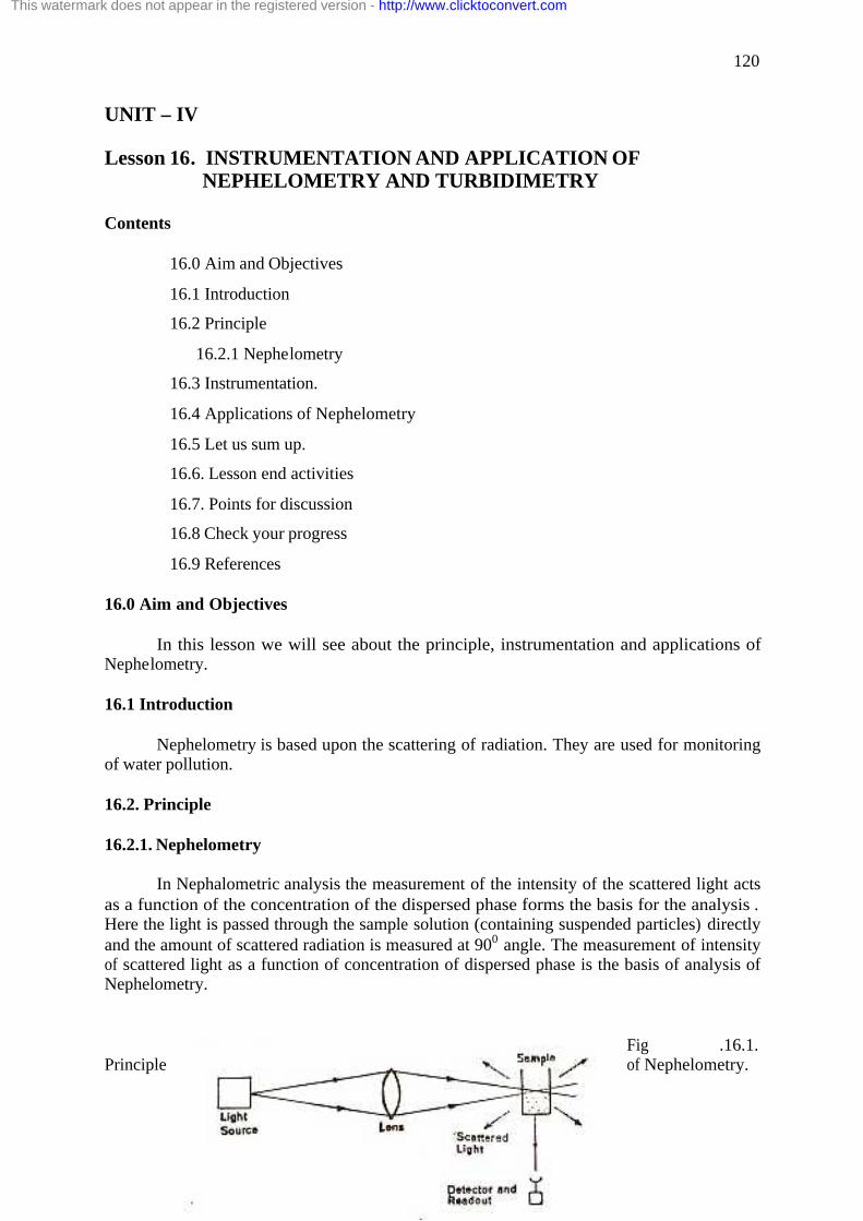
120

UNIT – IV

Lesson 16. INSTRUMENTATION AND APPLICATION OF NEPHELOMETRY AND TURBIDIMETRY Contents


16.1 Introduction

16.2 Principle

16.2.1 Nephelometry


16.4 Applications of Nephelometry

16.5 Let us sum up.




16.9 References 16.0 Aim and Objectives

In this lesson we will see about the principle, instrumentation and applications of Nephelometry. 16.1 Introduction

Nephelometry is based upon the scattering of radiation. They are used for monitoring of water pollution. 16.2. Principle 16.2.1. Nephelometry

In Nephalometric analysis the measurement of the intensity of the scattered light acts as a function of the concentration of the dispersed phase forms the basis for the analysis . Here the light is passed through the sample solution (containing suspended particles) directly and the amount of scattered radiation is measured at 900 angle. The measurement of intensity of scattered light as a function of concentration of dispersed phase is the basis of analysis of Nephelometry.

Fig .16.1.

Principle of Nephelometry.



121

Theory For these measurements, transmitted intensity I can be determined with the equation,

Log I0 / It = K’Ic. I0 – Intensity of Incident light It – Intensity of transmitted light C – Concentration of absorbing particles in the solution. I – thickness of the absorbing medium


1. Explain the principle behind the nephelometric measurements? ………………………………………………………………………………………………….. ………………………………………………………………………………………………….. ………………………………………………………………………………………………….. ………………………………………………………………………………………………….. ………………………………………………………………………………………………….. 16.3. Instrumentation

The instruments used in Nephelometry are similar to that used in Spectrophotometry.

Source : Generally a mercury arc with special filter combination is highly preferred. Cells : A cell with a rectangular cross section is usually selected for the study. The figure of such cell is shown in fig.16.2. Detectors: Phototubes are used in turbidimeters and photomultiplier tubes are used in Nephelometry. They are fixed on circular disc which allows measurement at 00C & from 350 to 1350.

Figure 16.2. Cell used in Nephelometric measurements 16.4. Applications of Nephelometry

1. They are of higher importance in water treatment plants, sewage work, power and steam generating plants, in beverage bottling industry, Paper & pulp industry, Petroleum refineries and in pharmaceutical industry.

2. In Water analysis, they are used to determine clarify and for understanding the efficiency of treatment process.



122

3. They are used to determine the Co2 concentration. (Ba salt + Co2 BaCo3 – analyzed by Nephelometry or turbidimetry.)

4. Turbidimetry is used to analyze turbidity in sugar products and citrus juices. 5. Nephelometry helps to determine the content of carbonate as BaCo3, Cl-, as AgCl, F

as CaF2, and Cyanide as AgCN. 6. These methods are more precise than colorimetric methods. For eg. ‘P’ can be

detected at a concentration of 1 ppm too.


2. Is it possible to measure the turbidity caused by the precipitate of BaSO4?

………………………………………………………………………………………………… ………………………………………………………………………………………………… ………………………………………………………………………………………………… ………………………………………………………………………………………………… ………………………………………………………………………………………………… ………………………………………………………………………………………………. 16.5 Let us sum up

Thus we have seen about

· Principle of Nephelometry · Instrumentation of Nephelometry · Its advantages · Its applications

16.6 . Lesson end activities

· Find out the abbreviation of NTU using relevant books. · Find the difference between scatterings is dispersion.


ü How Nephelometry does differ from turbidimetry? Explain

16.8 Check your progress For the question asked in the above section it is necessary to mention the principle of Nephelometry in detail. As we have discussed earlier you will not forget to mention about the principle of the instrument followed by the components applications as given below. You will give side headings as we have given in the lesson. 16.9 References 1. Surles, T., J. O. Erickson, and D. Priesner, Am. Lab., 7(3), 55 (March 1975). 2. Wendlandt, W.W., J. Chem. Educ., 45, A861, A947 (1968) 3. Dougles A Skoog and Donald M. West .Principles of Instrumental Analysis – 4. Eiassett. R.C.Denney, G.H. Jeffery, J. Mendham Voges .Text Book of Quantitative




123

Lesson 17. INSTRUMENTATION AND APPLICATION OF TURBIDIMETRY Contents


17.1 Introduction

17.2 Principle

17.2.1 Turbidimetry


17.4 Applications of Turbidimetry.

17.5 Let us sum up.




17.9 References


In this lesson we will see about the principle, instrumentation and applications of Turbidimetry. 17.1 Introduction

Turbidimetry is based upon the scattering of light by non-transparent suspended particles in the solution. However the method of measurement of the scattered radiation varies from that of Nephelometry. 17.2. Principle 17.2.1. Turbidimetry

When light is passed through the suspension, part of incident radiant energy is dissipated by absorption, refraction and reflection while remainder is transmitted. “The measurement of the intensity of transmitted light as a function of the concentration of dispersed phase is the basis of turbidimetric analysis.” Turbidimetry is more satisfactory for the determination of relatively high concentration of suspended particles.

Fig16.1 Principle of turbidimetry.



124

Theory

For these measurements, transmitted intensity I can be determined with the equation, Log I0 / It = K’Ic.

I0 – Intensity of Incident light It – Intensity of transmitted light c – Concentration of absorbing particles in the solution. I – thickness of the absorbing medium

K’- turbidity coefficient Self-Check Exercise 1

1. What is the basic difference between the functioning of Nephelometry and turbidimetry?

………………………………………………………………………………………………….. ………………………………………………………………………………………………….. ………………………………………………………………………………………………….. ………………………………………………………………………………………………….. ………………………………………………………………………………………………….. 17.3. Instrumentation

The instruments used in turbidimetry are similar to that used in Spectrophotometry.

Source : Generally a mercury arc with special filter combination is highly preferred. Cells : A cell with a rectangular cross section is usually selected for the study. Detectors: Phototubes are used in turbidimeters. They are fixed on circular disc which allows measurement at 00C & from 350 to 1350.

Fig.17.2 shows a simple turbidimeter, which consists of a cylinder to contain the turbid solution, a lamp filament of fixed intensity at the base and an adjustable plunger through which visual observation is made. The depth of turbid solution needed to extinguish the image of lamp is noted. A standard graph is prepared using standard suspension. The graph is drawn by plotting depth versus concentration. Fig.17.2.Simple turbidimeter



125

17.4. Applications of Turbidimetry

1. They are of higher importance in water treatment plants, sewage work, power and steam generating plants, in beverage bottling industry, Paper & pulp industry, Petroleum refineries and in pharmaceutical industry.

2. In Water analysis, they are used to determine clarify and for understanding the efficiency of treatment process.

3. They are used to determine the Co2 concentration. (Ba salt + Co2 BaCo3 – analyzed by Nephelometry or turbidimetry.)

4. Turbidimetry is used to analyze turbidity in sugar products and citrus juices. 5. Nephelometry helps to determine the content of carbonate as BaCo3, Cl-, as AgCl, F

as CaF2, and Cyanide as AgCN. 6. These methods are more precise than colorimetric methods. For eg. ‘P’ can be

detected at a concentration of 1 ppm too. 7. The turbidity caused by BaSO4 can be analysed using this instrument. The turbidity

could be set 100NTU using the standard solution(hydrazine sodium + hexamethylene tetra mine.).Then the BaSO4 solution can be fed to the instrument and the turbidity could be read directly.


2. Is it possible to measure the turbidity caused by the precipitate of BaSO4?

………………………………………………………………………………………………… ………………………………………………………………………………………………… ………………………………………………………………………………………………… ………………………………………………………………………………………………… ………………………………………………………………………………………………… 17.5 Let us sum up

Thus we have seen about

· Principle of Nephelometry and turbidimetry · Instrumentation of Nephelometry and turbidimetry · Their advantages · Their applications


· Draw a standard graph for the turbidity of standard solution prepared using hydrazine sodium + hexamethylene tetra mine.


ü How could you compare the values of turbidity obtained for clear drinking water and textile industry waste water?

ü Is it possible to analyze the turbidity caused by BaSo4? Explain.



126

17.8 Check your progress · For the first question you will first write the sentence that it is possible to compare the

values of turbidity obtained for clear drinking water and textile include waste water. Then high light the principle of the measurement of turbidity. Because this will make

you understand the reason for getting different values for different solutions so mention the principle as follows. When light is passed through the suspension, part of incident radiant energy is dissipated by absorption, refraction and reflection while remainder is transmitted. “The measurement of the intensity of transmitted light as a function of the concentration of dispersed phase is the basis of turbidimetric analysis.” Turbidimetry is more satisfactory for the determination of relatively high concentration of suspended particles. Later explain that the instrument used for the measurement of turbidity. Make a mention that as the light scattered will increase depending on the turbidity of the solution. The value of turbidity will be higher for industrial Waste waster and will be lesser for ordinary drinking water, which will be clear.

· For the second question high light the principle of the measurement of turbidity.

Because this will make you understand the reason for getting different values for different solutions so mention the principle as follows. When light is passed through the suspension, part of incident radiant energy is dissipated by absorption, refraction and reflection while remainder is transmitted. “The measurement of the intensity of transmitted light as a function of the concentration of dispersed phase is the basis of turbidimetric analysis.” Turbidimetry is more satisfactory for the determination of relatively high concentration of suspended particles.

Later explain that the instrument used for the measurement of turbidity. And then measurement procedure for BaSO4Could be mentioned as follows. The turbidity caused by BaSO4 can be analysed using this instrument. The turbidity could be set 100NTU using the standard solution(hydrazine sodium + hexamethylene tetra mine.).Then the BaSO4 solution can be fed to the instrument and the turbidity could be read directly. 17.9 References 1. Surles, T., J. O. Erickson, AND D. Priesner, Am. Lab., 7(3), 55 (March 1975). 2. Wendlandt, W.W., J. Chem. Educ., 45, A861, A947 (1968) 3. Dougles A Skoog and Donald M. West .Principles of Instrumental Analysis – 4. Eiassett. R.C.Denney, G.H. Jeffery, J. Mendham Voges .Text Book of Quantitative

Inorganic Analysis and Elementary Instrumental Analysis 5. Willard, Merril and Dean .Instrumental Methods of Analysis . 6. Chatwal and Anand .Instrumental Methods of Chemical analysis 7. B.K. Sharma .Instrumental Methods of Analysis



127

Lesson 18. INSTRUMENTATION AND APPLICATIONS OF CONDUCTOMETRY


18.1. Introduction



18.2.2 Specific Conductance

18.2.3 Electrical conductivity


18.3 Conductometric titrations

18.3.1 Replacement titrations

18.3.2 Precipitation titrations

18.3.3 Acid base titrations

18.3.4 Redox titrations

18.4. Other Applications of Conductometry

18.5 Let us sum up




18.9 References

18.0 Aims and Objectives In this lesson we will discuss about the principle, measurement and applications of Conductometry.

18.1. Introduction

Titration is process of chemical analysis in which the quantity, amount or concentration, of some constituent of a sample, known as an analyte, is determined by adding to the measured sample an exactly known quantity of another substance with which the desired constituent reacts in a definite, known proportion. The process is usually carried out by gradually adding a standard solution (i.e., a solution of known concentration) of titrating reagent, or titrant, from a burette, essentially a long, graduated measuring tube with a stopcock and a delivery tip at its lower end. Titrations may be carried out by hand from the burette or automatically.



128

At the equivalence point of a titration, an exactly equivalent amount of titrant has been added to the sample. The experimental point at which the completion of the reaction is marked by some signal is called the end point. This signal can be the colour change of an indicator or a change in some chosen, e.g., electrical property that is measured during the titration. The difference between the end point and the equivalence point is the titration error, which is kept as small as possible by the proper choice of an end-point signal and a method for detecting it.

For many titration reactions it is possible to find a suitable visual colour indicator that

will signal the end point at, or very close to, the equivalence point. Such titrations, classified according to the nature of the chemical reaction occurring between the sample and titrant, include: acid-base titrations, precipitation titrations, complex-formation titrations, and oxidation-reduction (Redox) titrations.


For many titrations the end point can be detected by electrical measurements. These

titrations may be classified according to the electrical quantity that is measured. Potentiometric titrations involve the measurement of the potential difference between two electrodes of a suitable cell; Conductometric titrations, the electrical conductance or resistance of the solution being titrated is being measured.


The specific resistance is defined as the resistance between opposite faces of one cm.

cube of the metal. The resistance of the conductor is directly proportional to its length and inversely proportional to the cross sectional area. Thus,

R a l/a R = ρ l/a

R=Resistance, ρ = Specific Resistance.. The unit of resistance is ohms and of specific resistance is ohm/cm. 18.2.2 Specific Conductance

The reciprocal of specific resistance is called specific conductance Specific conductance = 1/ ρ

18.2.3 Electrical Conductivity

It is defined as the conductivity in ohms of a solution containing one gm equivalent of

solute when placed between two sufficiently large electrodes, which are one cm apart. It is denoted by l. Self-Check Exercise 1

1. How will you calculate the resistance of a conductor? ………………………………………………………………………………………………….. ………………………………………………………………………………………………….. ………………………………………………………………………………………………….. ………………………………………………………………………………………………….. …………………………………………………………………………………………………..



129


The solution whose conductivity is to be determined is taken in a suitable cell, known as conductivity cell. These cells are made of quartz and are fitted with platinum electrodes. The electrodes usually consist of two sheets of platinum. In order to remove the polarization effects the electrodes are coated with finely divided platinum black, and these are called platinized platinum electrodes. The measurement of conductivity using a conductivity meter involves the measurement of cell constant of the conductivity cell. The cell is first calibrated with 0.1 N KCl solutions, following which the conductance of the unknown solution can be measured in mhos.

The determination of the end point of a titration with the help of conductivity

measurements is termed as Conductometric titrations.In a Conductometric titration, the titrant is added from the burette and the conductivities are plotted against the volume of the titrant in c.c. since the measured conductivity is a linear function of the concentration of ions present, two lines will be obtained which will intersect each other at a point, known as “end point” or “equivalence point”

At times, hydrolysis, dissociation of the product may result in curvature near the end point. And conductivity is defined as the ease with which the current flows through a conductor. Hence it is the reciprocal of resistance.

C = (1 / R) unit is mhos.

18.3 Types of Conductometric titrations The Conductometric titrations depends on the measurement of the conductivity of the

ions present in solution. The two factors involved are the concentration and speed of the ions. 18.3.1 Replacement titrations

When a strong acid reacts with sodium or potassium salts of weak acid, the ion of weak acid is replaced first consider the titration of sodium acetate with hydrochloric acid. CH3COO-Na+ + H+Cl- CH3COO-H+ + Na+Cl-. In this titration only a slight increase in conductance is obtained up to the end point. This is because of the fact that chloride ion has higher conductance than the acetate ion. After the end point, it increases more rapidly, due to the addition of excess of HCl (Fig.18. 1). This is used in the determination of alkaloids. Fig.18.1.Curve obtained for Replacement titrations conductivity Precipitant added



130

18.3.2. Precipitation titrations They cannot be carried out so effectively as acid-base titrations. Consider the reaction taking place between KCl & AgNo3.

[ K+ + Cl- ] + [ Ag+ + No3- ] [ K+ + No3

- ] + Agcl.] In the initial stages of the titration, with the addition of AgNo3, the conductance does not change much. This is because the cl- tons are replaced by No3

- ions and both have same ionic conductance. After the end point, the excess of AgNo3 added causes a sharp increase in the conductance (Fig.18. 2) Fig.18.2.Curve obtained for the precipitation titration conductivity Precipitant added 18.3.3. Acid – base titrations (i) Strong acid us strong base: Let us consider the titration of Hcl with NaoH. [H+Cl-] + [Na+OH-] [Na+Cl-] + H2O.

Initially, acid solution has high conductivity due to highly mobile hydrogen ions. The

share due to chloride ions will be smaller due to less mobility as compared to hydrogen. When NaoH is added to Hcl, the highly mobile hydrogen ions are replaced by less mobile Na+ ions. This will result in the decrease of conductivity.

At the end point the conductivity will be a minimum due to Na+ & cl- ions. Further

Addition of NaoH will increase the conductivity due to OH- ions. (Fig.18. 3) Fig.18.3.Curve obtained for the titration of strong acid vs strong base

conductivity Volume of NaoH added (ii) Strong acid with a weak base:



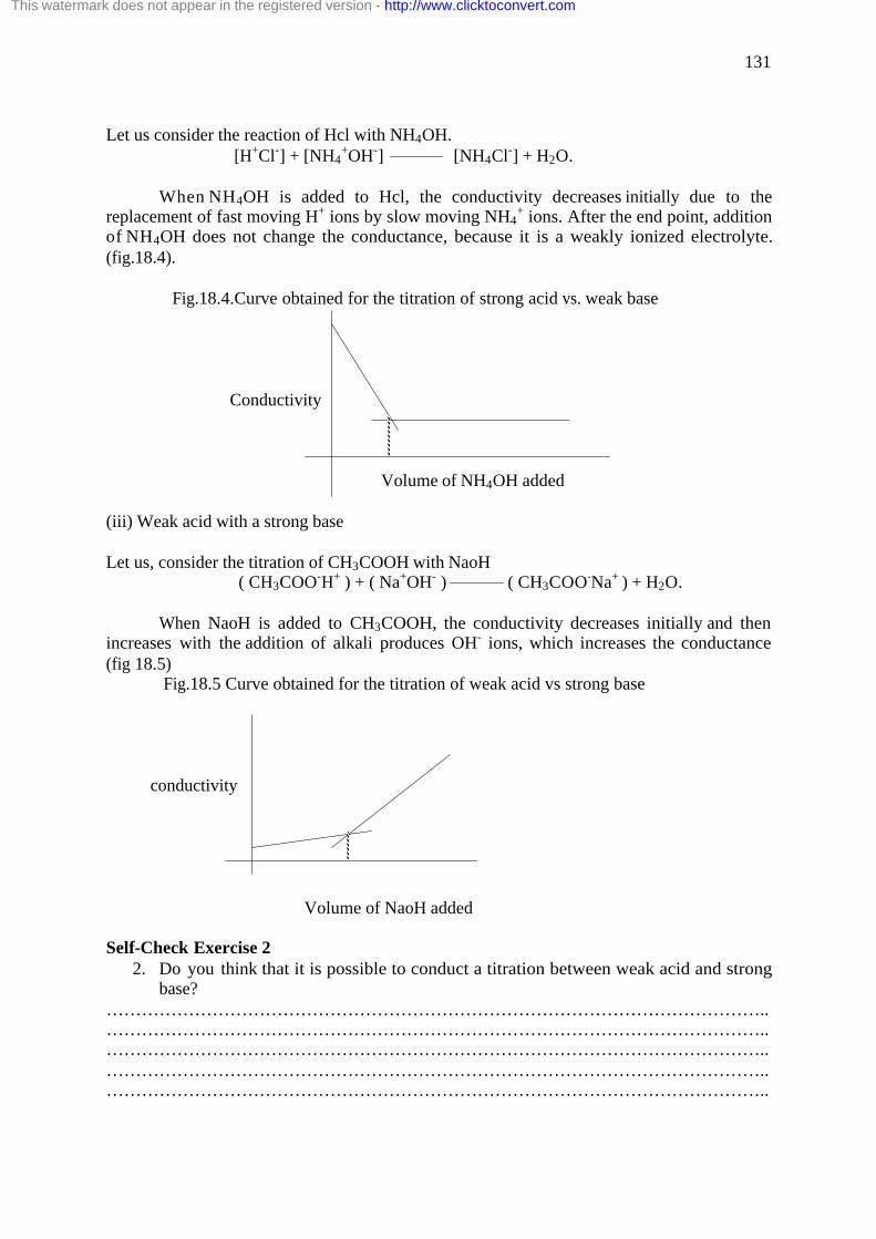
131

Let us consider the reaction of Hcl with NH4OH. [H+Cl-] + [NH4

+OH-] [NH4Cl-] + H2O.

When NH4OH is added to Hcl, the conductivity decreases initially due to the replacement of fast moving H+ ions by slow moving NH4

+ ions. After the end point, addition of NH4OH does not change the conductance, because it is a weakly ionized electrolyte. (fig.18.4).

Fig.18.4.Curve obtained for the titration of strong acid vs. weak base

Conductivity Volume of NH4OH added (iii) Weak acid with a strong base Let us, consider the titration of CH3COOH with NaoH ( CH3COO-H+ ) + ( Na+OH- ) ( CH3COO-Na+ ) + H2O.

When NaoH is added to CH3COOH, the conductivity decreases initially and then

increases with the addition of alkali produces OH- ions, which increases the conductance (fig 18.5) Fig.18.5 Curve obtained for the titration of weak acid vs strong base conductivity Volume of NaoH added Self-Check Exercise 2

2. Do you think that it is possible to conduct a titration between weak acid and strong base?

………………………………………………………………………………………………….. ………………………………………………………………………………………………….. ………………………………………………………………………………………………….. ………………………………………………………………………………………………….. …………………………………………………………………………………………………..



132

18.3.4. Redox Titrations

In the case of oxidation – reduction titrations, there is a decrease in the hydrogen ion concentration as follows:

6Fe2+ + Cr2O72- + 14H+ 6Fe3+ + 7Cr3+ + 7H2O.

Since the mobility of hydrogen ion is high, so a sharp decrease in the conductance is

expected during the initial part of the titration. After the end point the conductance remains the same.

Fig.18.6.Curve obtained for the redox titration conductivity Volume of NaOH added 18.4 Other Applications of Conductometry

Conductometric measurements are widely used for the analysis of salinity of sea water in oceanographic work. They are useful in providing information regarding association or dissociation equilibria in aqueous solutions, provided that one or more of the reacting species are ionic. Conductivity bridges with special electrodes for specific purposes, like estimation of ash content in sugar juices, moisture content of wood for pulping purposes have been devised.


3. Is it possible to measure the conductance of sugar solution? Will the conductance be the same as that of ordinary water?

………………………………………………………………………………………………… ………………………………………………………………………………………………… ………………………………………………………………………………………………… ………………………………………………………………………………………………… 18.5. Let us sum up

Thus we have seen about · Principle of Conductometry · Instrumentation of Conductometry · Their advantages · Their applications



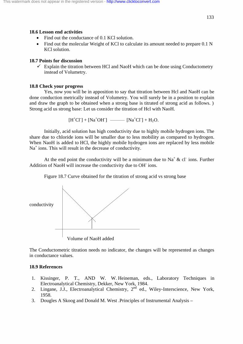
133

18.6 Lesson end activities · Find out the conductance of 0.1 KCl solution. · Find out the molecular Weight of KCl to calculate its amount needed to prepare 0.1 N

KCl solution. 18.7 Points for discussion ü Explain the titration between HCl and NaoH which can be done using Conductometry

instead of Volumetry.

18.8 Check your progress Yes, now you will be in apposition to say that titration between Hcl and NaoH can be

done conduction metrically instead of Volumetry. You will surely be in a position to explain and draw the graph to be obtained when a strong base is titrated of strong acid as follows. ) Strong acid us strong base: Let us consider the titration of Hcl with NaoH. [H+Cl-] + [Na+OH-] [Na+Cl-] + H2O.

Initially, acid solution has high conductivity due to highly mobile hydrogen ions. The share due to chloride ions will be smaller due to less mobility as compared to hydrogen. When NaoH is added to HCl, the highly mobile hydrogen ions are replaced by less mobile Na+ ions. This will result in the decrease of conductivity.

At the end point the conductivity will be a minimum due to Na+ & cl- ions. Further

Addition of NaoH will increase the conductivity due to OH- ions. Figure 18.7 Curve obtained for the titration of strong acid vs strong base

conductivity Volume of NaoH added

The Conductometric titration needs no indicator, the changes will be represented as changes in conductance values. 18.9 References 1. Kissinger, P. T., AND W. W. Heineman, eds., Laboratory Techniques in

Electroanalytical Chemistry, Dekker, New York, 1984. 2. Lingane, J.J., Electroanalytical Chemistry, 2nd ed., Wiley-Interscience, New York,

1958. 3. Dougles A Skoog and Donald M. West .Principles of Instrumental Analysis –



134

4. Eiassett. R.C.Denney, G.H. Jeffery, J. Mendham Voges .Text Book of Quantitative Inorganic Analysis and Elementary Instrumental Analysis

5. Willard, Merril and Dean .Instrumental Methods of Analysis. 6. Chatwal and Anand .Instrumental Methods of Chemical analysis 7. B.K. Sharma .Instrumental Methods of Analysis.



135

Lesson 19. ION SELECTIVE ELECTRODES Contents


19.1. Introduction

19.2. Types of electrode system.

19.3. Ion selective electrodes

19.3.1 The glass electrode

19.3.2 Polymer membrane electrode

19.3.3 Solid state electrode

19.3.4 Gas membrane electrode

19.4 Applications of Ion selective electrodes.

19.5 . Let us sum up




19.9 References


In this lesson we will see about the ion selective electrodes, their types along with their applications.

19.1 Introduction

Ion selective electrodes have become important in recent years as they are widely used for clinical, biological, water, air, oceanographic and pharmaceutical research. An Ion-selective electrode (ISE) is a transducer ( sensor) which converts the activity of a specific ion dissolved in a solution into an electrical potential which can be measured by a voltmeter

or pH meter. The voltage is theoretically dependent on the logarithm of the ionic activity, according to the Nernst equation. The sensing part of the electrode is usually made as an ion-specific membrane, along with a reference electrode. Ion-selective electrodes are used in biochemical and biophysical research, where measurements of ionic concentration in an aqueous solution are required, usually on a real time basis. 19.2. Types of electrode system

Electrode systems can be divided into different classes depending on the species that

determine the electrode potential. The indicator electrodes are either made of noble metals such as Pt or Au, insoluble metal salt/metal electrode (Agcl/Ag) or ion selective electrodes.


http://en.wikipedia.org/wiki/Sensor

http://en.wikipedia.org/wiki/Activity_%28chemistry%29


http://en.wikipedia.org/wiki/Solution

http://en.wikipedia.org/wiki/Potential

http://en.wikipedia.org/wiki/Voltmeter

http://en.wikipedia.org/wiki/PH_meter

http://en.wikipedia.org/wiki/Logarithm

http://en.wikipedia.org/wiki/Nernst_equation

http://en.wikipedia.org/wiki/Electrode

http://en.wikipedia.org/wiki/Artificial_membrane

http://en.wikipedia.org/wiki/Reference_electrode

http://en.wikipedia.org/wiki/Biochemistry

http://en.wikipedia.org/wiki/Biophysics


http://en.wikipedia.org/wiki/Concentration

http://en.wikipedia.org/wiki/Aqueous_solution


136

Nobel metal electrodes In these electrodes the noble metal used is the insert metal, Pt. It acts as the indicator

electrode. This in combination with a reference electrode constitutes a cell. The inert electrode acts as a site of electron transfer. The inert metal pt does not take part in the electrochemical half cell reaction but acts as a collector of electrodes.

For eg. Pt, H2/H+ represents the hydrogen electrode, with Pt acting as an inert

electrode. Insoluble metal salt/metal electrodes: In these electrodes the metal electrode is in

contact with a slightly soluble salt. The example of this type of electrode is Ag / Agcl, cl-. This electrode responds to changes in the anion (cl-) concentration. If the

concentration of the anion is constant, electrodes may be called as reference electrode eg., saturated calomel electrode, which is obtained by preparing saturated Kcl solution. 19.3. Ion Selective Electrodes

The ion selective electrodes possess the electrode which acts as a collector or donor of electrons. Several types of sensing electrodes are commercially available. They are classified by the nature of the membrane material used to construct the electrode. It is this difference in membrane construction that makes an electrode selective for a particular ion. But certain substances not only collect the electrons, but also take part in the half cell reaction. For example, a zinc rod responds to Zn2+, copper rod responds to cu2+ and mercury to Hg2+ ions. These metals can act as ion selective electrodes.

A pair of electrode (ion selective electrode and reference electrode) may be dipped into a solution of the substance to be determined and concentration of the sample can be obtained from the observed potential.


1. Which metal acts inert thereby it is used in electrode construction? ………………………………………………………………………………………………….. ………………………………………………………………………………………………….. ………………………………………………………………………………………………….. ………………………………………………………………………………………………….. …………………………………………………………………………………………………..

19.3.1. The Glass Electrode.

The glass electrode is meant for the measurement of pH. This electrode consists of a

small bulb of pH sensitive glass containing a buffered chloride solution and an internal reference electrode used is silver- silver chloride or calomel. The glass calomel electrode system is a remarkably versatile tool for the measurement of pH under many conditions



137

Fig.19. 1. Glass electrode.

Legend

1. a sensing part of electrode, a bulb made from specific glass

2. sometimes electrode contain small amount of AgCl precipitate inside the glass electrode

3. internal solution, usually 0.1M HCl for pH electrodes 4. internal electrode, usually silver chloride electrode or

calomel electrode 5. body of electrode, made from non-conductive glass or

plastics. 6. reference electrode 7. junction with studied solution, usually made from

ceramics or capillary with asbestos or quartz fiber.

19.3.2. Polymer Membrane Electrodes (Organic Ion Exchangers and Chelating Agents) –

Polymer membrane electrodes consist of various ion-exchange materials incorporated into an inert matrix such as PVC, polyethylene or silicone rubber. After the membrane is formed, it is sealed to the end of a PVC tube. The potential developed at the membrane surface is related to the concentration of the species of interest. Electrodes of this type include potassium, calcium, chloride, and fluoroborate, nitrate, per chlorate, potassium, and water hardness.

19.3.3. Solid State Electrodes Solid state electrodes utilize relatively insoluble inorganic salts in a membrane. Solid state electrodes exist in homogeneous or heterogeneous forms. In both types, potentials are developed at the membrane surface due to the ion-exchange process. Examples include silver/sulphide, lead, copper (II), cyanide, thiocyanate, chloride and fluoride. 19.3.4 Gas Membrane Electrodes

Gas sensing electrodes are available for the measurement of dissolved gas such as ammonia, carbon dioxide, nitrogen oxide, and sulfur dioxide. These electrodes have a gas permeable membrane and an internal buffer solution. Gas molecules diffuse across the membrane and react with a buffer solution, changing the pH of the buffer. The pH of the buffer solution changes as the gas reacts with it. The change is detected by a combination pH



138

sensor within the housing. Due to the construction, gas sensing electrodes do not require an external reference electrode.

19.4. Applications of Ion selective Electrodes

The use of Ion Selective Electrodes in environmental analysis offer several advantages over other methods of analysis. First, the cost of initial setup to make analysis is relatively low.

Calcium electrode has been used to determine Ca2+ ton in milk, sea water, beer, boiler

water, sugar, wine etc. As the ton is one of the most important in human physiology, its determination is important.

Ammonia electrode would help to determine the concentration of NH3 reducing the

complication of Kjeldahl N2 determination. Chloride electrode is used for the analysis of industrial and physiological samples. Lead can be measured in blood, urine samples with Pbs/Ag2S electrode. These electrodes are found to be easy to use, available in different shapes and sizes

and are of nominal cost.


2. What is the difference between ordinary electrode and ion selective electrodes? ………………………………………………………………………………………………… ………………………………………………………………………………………………… ………………………………………………………………………………………………… ………………………………………………………………………………………………… ………………………………………………………………………………………………… ………………………………………………………………………………………………… 19.5. Let us sum up

In this lesson we have discussed about the · Ion selective electrodes · Electrode systems · Glass electrodes · Liquid membrane electrodes · Double membrane electrodes · Solid state electrodes

19.6 Lesson end activities · Add KMno4 to KI slowly. Check the colour change visually. · Practice preparing a salt bridge. It must have a uniform edge.



139

19.7 Points for discussion ü How will perform an experiment to determine the pH of given dyeing industry

effluent.

19.8 Check your progress In the lesson on ion selective electrode you have studied that the pH of the solution

could be analyzed using glass electrode. You have to mention the principle of the instrument, working mechanism as below. The glass electrode is meant for the measurement of pH. This electrode consists of a small bulb of pH sensitive glass containing a buffered chloride solution and an internal reference electrode used is silver- silver chloride or calomel. The glass calomel electrode system is a remarkably versatile tool for the measurement of pH under many conditions

Fig. Measurement of pH with glass electrode.

19.9 References 1. Bates, R.G., Determination of pH: Theory and Practice, 2nd ed., John Wiley, New York,

1973. 2. Freiser, H., ed., Ion-Selective Electrodes in Analytical Chemistry, Vol. 2, Plenum Press,

New York, 1980. 3. Koryta, J., AND K. Stulik, Ion-Selective Electrodes, 2 nd ed., Cambridge University

Press. Cambridge, U.K., 1983. 4. Ma, T.S., and S.S.M. hassan, Irganic Analysis Using Ion-Selective Electrodes, Vols, 1

and 2, Academic, London, 1982. 5. Rechnitz, G. A., “Bio analysis with Potentiometric Membrane Electrodes,” Anal.

Chem., 54, 1194A (1982). 6. Dougles A Skoog and Donald M. West .Principles of Instrumental Analysis – 7. Eiassett. R.C.Denney, G.H. Jeffery, J. Mendham Voges .Text Book of Quantitative





140

Lesson 20. INSTRUMENTATION AND APPLICATIONS OF POTENTIOMETRY Contents


20.1 Introduction

20.2. Potentiometric measurements


20.4. Applications of Potentiometric titrations

20.5. Types of Potentiometric titrations

20.5.1. Acid base titrations

20.5.2. Redox titrations

20.5.3. Precipitation titrations

20.6. Advantages of Potentiometric titrations





20.11 References

20.0 Aims and Objectives In this we shall discuss about Potentiometric measurements, its instrumentation, applications of Potentiometric titrations, types of such titrations and advantages. 20.1. Introduction

If, during a chemical reaction, there is a change in the concentration of an ion which can be sensed through the change in potential of a suitable electrode, then the progress of the reaction can be followed through this potential change. It follows the electromotive force measurements, like conductivity measurements, can serve to determine the equivalence point or end point of titration. Both conventional electrodes and the types of ion-sensitive electrodes can be used to follow the process and the change of potential in the case of acid-base, precipitation, complexation and Redox titration. 20.2. Potentiometric measurements

In Potentiometric methods two methods of measurements exists. A) Measurement of electrode potential from which the concentration of an active ion

may be found.



141

B) Measurement of changes in E.M.F.(electro motive force) brought about by the addition of the titrant could be made.

Thus the E.M.F. of the cell can be calculated as follows. E cell = E reference + E indicator + E function E cell = E H2 / H + E J + E Agcl / Ag

When hydrogen electrode becomes reference electrode its potential becomes zero, thus E cell = E J + E Agcl / Ag E J, arises across the liquid- liquid boundary or salt bridge due to unequal migration of

ions. The potential is kept either low or constant during the titration. Thus the e.m.f. of the cell is equal to the numerical value of the potential of silver, silver chloride electrode (indicator electrode).

In Potentiometric titrations, the change in the electrode potential upon the addition of

the titrant are noted against the volume of the titrant & added. At the end point the rate of the change of the potential would be the maximum. The end point is found by plotting a curve of potential versus the volume of the titrant. Self-Check Exercise 1

1. What is an E.M.F? ………………………………………………………………………………………………….. ………………………………………………………………………………………………….. ………………………………………………………………………………………………….. ………………………………………………………………………………………………….. ………………………………………………………………………………………………….. 20.3. Instrumentation

There are three types of instruments which are generally used for the measurement of e.m.f. Non – Electronic instruments.

Electronic instruments and Automatic instruments

20.4. Applications of Potentiometric titrations.

During the titration, the potential of the cell is measured after each addition of the solution. Time is allowed for the attainment of equilibrium. This methodology is useful for many titrations. 20.5. Types of Potentiometric titrations

Potentiometric titrations are applied to a variety of systems including acid base titrations, Redox titrations and precipitation titrations. 20.5.1. Acid base titrations

It is clear that neutralization of acids & bases is always accompanied by the changes in the concentration of H+ & OH- ions. The electrodes used are hydrogen electrode & N-



142

calomel electrode (Reference electrode). The glass electrode is usually used in conjunction with a calomel electrode that makes contact with the test solution through a salt bridge.

Fig.20. 1.Apparatus used for acid-base titration. A known volume of the acid to be titrated is kept in a beaker fitted with a stirrer and a

standard hydrogen electrode. It is connected to normal calomel electrode through a salt bridge. Both the electrodes are connected to a potentiometer which records the E.M.F. of the solution. After each addition of base from the burette, the E.M.F is measured & a graph is plotted (fig.20.2)

Fig.20.2.Graph obtained by plotting volume vs E.M.F E.M.F V The potential of any hydrogen electrode is given by E = E0 + 0.0591 pH. It is clear that the change in electrode potential or E.M.F. of the cell is proportional to

the change in pH during titration. The point where the E.M.F. increases rapidly gives the end point.A more satisfactory method to find the end point is to plot ∆E/∆V against V. The maximum value gives the end point of the titration (fig.20.3)

Fig.20.3.Graph obtained by plotting volume vs E/ V E/ V V



143

20.5.2. Redox Titrations

Redox reactions can be followed by an inert indicator electrode. The electrode assumes a potential proportional to the concentration of the reactant or the titrant. They involve the transfer of electron from the substances being oxidized to the substance being reduced.

Ce4+ + Fe2+ Ce3+ + Fe3+ Such reaction consists essentially of two half reactions whose standard potential may

be used to calculate the standard potential of the reaction. Fe2+ Fe3+ + e- E0 = -0.76 V (1) Ce4++e- Ce3+ E0 = + 1.61V (2) Ce4++ Fe2+ Fe3+ + Ce3+ E0 = + 0.851V (3) Such titrations may be used for monitoring of cyanide wastes from metal plating

industries, in water pollution, sewage treatment, agricultural and in biochemical studies. 20.5.3. Precipitation titrations

Any such titration that involves insoluble salts of metals such as mercury, silver lead and copper may be followed potentiometrically. The indicator electrode may be made of the metal involved in the reaction. The magnitude of potential change at the end point depends on the solubility of the substance being precipitated. The titration of Cl- ions with a stand and solution of AgNo3 using a silver metal indicator electrode is an example of a precipitation titration. 20.6. Advantages of Potentiometric titrations

1. The method is suitable for the analysis of dilute solutions too. 2. It could be applied for colored solutions also. 3. The interpretation of titration curves is easier. 4. The apparatus used is inexpensive, reliable and readily available. 5. Different components of different characteristic colour could be titrated at a same

time.


2. Is it possible to find out the end point of an acid base titration using a potentiometer? ………………………………………………………………………………………………… ………………………………………………………………………………………………… ………………………………………………………………………………………………… ………………………………………………………………………………………………… …………………………………………………………………………………………………. …………………………………………………………………………………………………



144

20.7. Let us sum up In this lesson we have discussed about

· Potentiometry · Potentiometric measurements · Instrumentation · Applications · Types of titrations done using Potentiometry · Advantages

20.8 Lesson end activities · Check the various electrodes available to conduct Conductometric and

Potentiometric titrations.

20.9 Points for discussion ü Can you estimate the amount of Agcl present in the given solution?

20.10 Check your progress For the question it is very clear that you have to describe the usage of

Potentiometric titration clearly. It is also possible to analyze the amount of Agcl present in the given solution using precipitation titration. Any such titration that involves insoluble salts of metals such as mercury, silver lead and copper may be followed potentiometrically. The indicator electrode may be made of the metal involved in the reaction. The magnitude of potential change at the end point depends on the solubility of the substance being precipitated. The titration of Cl- ions with a stand and solution of AgNo3 using a silver metal indicator electrode is an example of a precipitation titration. 20.11 References 1. Bates, R.G., Determination of pH: Theory and Practice, 2nd ed., John Wiley, New York,

1973. 2. Freiser, H., ed., Ion-Selective Electrodes in Analytical Chemistry, Vol. 2, Plenum Press,

New York, 1980. 3. Koryta, J., and K. Stulik, Ion-Selective Electrodes, 2nd ed., Cambridge University Press.

Cambridge, U.K., 1983. 4. Ma, T.S., and S.S.M. hassan, Inorganic Analysis Using Ion-Selective Electrodes, Vols,

1 and 2, Academic, London, 1982. 5. Rechnitz, G. A., “Bio analysis with Potentiometric Membrane Electrodes,” Anal.

Chem., 54, 1194A (1982). 6. Dougles A Skoog and Donald M. West .Principles of Instrumental Analysis – 7. Eiassett. R.C.Denney, G.H. Jeffery, J. Mendham Voges .Text Book of Quantitative

Inorganic Analysis and Elementary Instrumental Analysis 8. Willard, Merril and Dean .Instrumental Methods of Analysis . 9. Chatwal and Anand .Instrumental Methods of Chemical analysis

10. B.K. Sharma .Instrumental Methods of Analysis



145

UNIT – V

Lesson 21 COLLECTION AND PRESENTATION OF DATA Contents


21.1. Introduction

21.2. Data Collection

21.2.1 Primary data

21.2.2 Secondary data

21.3. Sources of primary and secondary data

21.3.1. Methods of collecting primary data

21.3.1.1 Direct personal investigation

21.3.1.2 Indirect oral investigation

21.3.1.3 Information from correspondents

21.3.2. Methods of collecting secondary data

21.3.3. Methods of data Collection

21.4. Classification of data

21.4.1. Types of classification

21.4.1.1 Geographical classification

21.4.1.2 Chronological classification

21.4.1.3 Qualitative classification

21.4.1.4 Qualitative classification

21.5. Tabulation of data

21.6. Diagrammatic representation of data

21.6.1. Bar diagram

i) Simple bar diagram

ii) Subdivided bar diagram

iii) Multiple bar diagram

iv) Percentage bar diagram

21.6.2. Pie diagram

21.7. Graphical representation of data

21.7.1. Histogram

21.7.2. Frequency polygon



146


21.7.4. O give Curve

21.8. Let us sum up

21.9. Lesson end activities 21.10. Points for discussion 21.11. Check your progress 21.12. References

21.0 Aims and objectives

This lesson deals with the collection, tabulation of data along with the representation of data.(rules for construction and types of diagram and graphs). 21.1. Introduction

Statistical methodology has been used in all disciplines of social sciences, pure and applied sciences, as well as in several areas of humanities. It covers all fields of study where in quantitative data appear and need analysis. In statistical study, there is an operation of multiple causes and the investigator has only limited control over consequences of a situation. 21.2. Data Collection

Data constitutes the foundation for statistical analysis. Facts expressed in quantitative form can be termed as data. Success of any statistical investigation depends on the availability of accurate and reliable data. These depend on the appropriateness of the method chosen for data collection. The data to be used can be of two types viz.

i) Primary data and ii) Secondary data

21.2.1 Primary data

The primary data is the one which has already been collected by a source other than the present investigator; for example, data obtained in the department of environment under the control of Ministry of Environment is a primary data. 21.2.2 Secondary Data

The Secondary data is one that has already been collected by a source other than the present investigator; for example, for the water board the details regarding water consumption would be given by public health department. Such data is secondary.

The difference between primary and secondary data is only in terms of degree. For

example, data, which is primary in the hands of one, become secondary in the hands of another. This distinction can be determined on the basis of the different criteria, as shown in the table 21.1



147

Table.21.1. Distinction between Primary and Secondary Data

S.No Basis Primary Data Secondary Data 1 Originality As the investigator himself

collects the data, it is original,

It is usually not original, since the investigator makes use of the data collected by other agencies.

2 Expenses It involves investment of time, energy and money

It is a comparatively cheaper method.

3 Suitability Its suitability will be positive

Its suitability may be positive or negative.

21.3. Sources of Primary and Secondary Data 21.3.1. Methods of collecting Primary Data

The main methods of collecting the primary data are as follows. 1. Direct personal investigation 2. Indirect oral investigation 3. Information from correspondents 4. Mailed questionnaire method.

These methods are discussed below.

21.3.1.1 Direct Personal investigation

The investigator has to contact the sources of information directly and personally. This method of collecting data is suitable: (a) when the area of investigation is limited, where the area of investigations is complex and heterogeneous, where a greater degree of intellectual power, experience and labor are required and also when a higher degree of accuracy is needed.

21.3.1.2 Indirect oral investigation

There are certain situations when the investigators cannot be approached directly. In such situations we have to collect data from those persons who may possess some knowledge about the investigations. This method is suitable in: (a) when the area of investigation is very large, (b) when the degree of accuracy is only of secondary importance.

21.3.1.3 Information from correspondents

In this method the investigator does not collect the information directly from the respondent. The task is handed over to a few persons or a group of persons, who are known as correspondents. The method is suitable in: When the area of investigation is very large. This method is generally employed by newspaper, magazine and various governmental agencies requiring information on regular basis.

21.3.1.4 Mailed questionnaire method

A questionnaire consists of a number of questions. Often a blank space is provided for the answer. The questions may be either descriptive type or objective type. It may be used to collect the data.



148

21.3.2. Methods of Collecting Secondary Data

The chief sources of secondary data can be classified into two groups.

i. Published sources ii. Unpublished sources.

21.3.3. Methods of data collection.. The methods of data collection could be done by the diagrammatically represented as follows: Fig.21.1 Methods of Data Collection. Self-Check Exercise 1

1. Are diagrammatic representations of data more appreciable than the tabulation of data?

………………………………………………………………………………………………….. ………………………………………………………………………………………………….. ………………………………………………………………………………………………….. ………………………………………………………………………………………………….. ………………………………………………………………………………………………….. 21.4. Classification of Data Classification

The collected data need to be classified to make the data fit for analysis and interpretation. The first step in the analysis and interpretation of data is the classification and tabulation. After the data has been systematically collected and edited, the first step in presentation of data is classification. Classification is the process of arranging the data according to the points of similarities and dissimilarities. It is like the process of sorting the

Methods of Data Collection

Census Method Sampling Method

Random

Simple Random Sampling

Purposive Mixed Sampling

Stratified Random

Sampling Systematic Random Sampling



149

letters in a post office where the letters for different destinations is placed in different compartments after it has been carefully sorted out from the huge heap.

The objectives of classification are to condense the mass of data to present the facts in simple form. to facilitate comparison and to facilitate the statistical treatment of the data.

21.4.1. Types of Classification

Some of the common types of classification are:

1. Geographical i.e., according to area or region. 2. Chronological i.e., according to occurrence of an event in time. 3. Qualitative i.e., according to attributes. 4. Quantitative i.e., according to magnitude.

21.4.1.1 Geographical Classification

The classification is based on the geographical region like countries, states, districts, etc. for example, the area of agricultural produce affected by smog per hectare for different countries in a particular year is

Table.21.2. Amount of agricultural product affected by Smog

Country Amount(Kg) USA 600 Canada 300 India 250 China 150

21.4.1.2 Chronological classification

This is based on the time of its occurrence such as years, months, weeks, etc.

For e.g., The fish (Catla catla) production in a particular farm over 5 years is

Table.21.3 Fish Production

Year Fish production (in kg/hectare) 1987 1400 1988 1500 1989 1550 1890 1600 1991 1650

21.4.1.3 Qualitative Classification

This is based on the quality such as sex, literacy, marital status etc.



150

It is further divided into two types. i. Simple classification ii. Manifold classification

I. Simple classification

The data are classified into two classes. Eg.

Population Population

Male Female Married Unmarried

II Manifold classification

The data are classified into many classes. Eg.

Population

Male Female

married unmarried married unmarried

21.4.1.4 Quantitative classification

This is based on some quantitative phenomena such as age, height etc. for example the weight of 100 fishes reared in a pond are Table.21.4. Weight of 100 fishes

Weight(gms) No. of fishes 0-100 18

100-200 16 200-300 20 300-400 12 400-500 20 500-600 13 600-700 6 700-800 1 800-900 2 900-1000 2

100 Self-Check Exercise 2

2. What are the common types of classification of data ? ………………………………………………………………………………………………….. …………………………………………………………………………………………………..



151

………………………………………………………………………………………………….. ………………………………………………………………………………………………….. ………………………………………………………………………………………………….. 21.5. Tabulation of Data

Tabulation may be defined as the logical and systematic arrangement of statistical data in rows and columns. It is designed to simplify presentation and facilitate comparison and analysis of the data. Structure of a Table

A table has the following parts. 1) Table number 2) Title 3) Caption 4) Sub heading 5) Body.

Raw Data The statistical information collected form the investigation is known as raw data. Suppose we are interested in the weight measurements of students of final M.Sc., Environmental sciences girls in this class. Their weight measurements are recorded as follows in Table.

Table.21.5 Weight of Environmental Sciences students

176 156 153 146 166 153 140 166 150 140

146 135 142 138 142 148 138 146 135 150

In the above table we have 20 observations relating to the weight measurements of 20 students. This data is known as raw data.

Discrete series

In order to understand the nature of discrete series, we must understand frequency. By frequency we mean the number of times a particular observation occurs, if we find that there are two students whose weight is 135 lb. We need not write 135 four times, rather we can simply say that the frequency of the value 135 is two. In a discrete series the units and their related frequency are given.

Table.21.6. Discrete Series Weight in (lb) 135 13 8 140 142 146 148 150 153 156 166 176

Frequency 2 2 2 2 3 1 2 2 1 2 1

Continuous series The units are expressed in various classes and their respective frequencies are given.

Construction of continuous series

The following steps are involved while constructing the series.



152

i) Determining the range It is obtained by subtracting the size of the smallest item from the size of the largest

item of the observed values. For example, in the above table the smallest value is 135 and the highest value is 176. Thus the range will be

176-135=41.

ii) Determining the number of classes There is no general rule governing the number of classes in a series. It can be

obtained by dividing the range by the size of the class interval. Two things need to be kept in consideration while determining the number of classes.

(a) Number of classes should neither be very large nor very small. In practice, we can have 5 to 15 classes; (b) the size of the class-internal should be an easy figure like 5, 10, 15,…

iii) Determination of class limit

We can make use of two methods, namely a) exclusive method b) inclusive method (non-overlapping)

In the exclusive method, the class- intervals are formed in the following manner.

120-130, 130-140…

The class 120-130 will mean that it includes values 120 or more than 120 but less than 130. Thus, the value 129 will be recorded in this class; the value 130 will not be recorded here. It will be recorded in 130-140.

In the inclusive method, the class intervals are formed as follows.

120-129, 130-139…

iv) Mid-Value The middle value of the class limits of a class interval is called the mid value of

class interval. Mid-value can be found by dividing the sum of lower and upper limit of the class- interval by two. For example, the sum of lower and upper limit of the class- interval by two. For example, the mid value of 120-130 will be

(120 + 130) / 2 = 250/2 = 125

Example : Continuous series (exclusive method) and (inclusive method)

Table:21.7 Continuous series (Exclusive method) weight of 20 girls (Ibs) Weight / Class- interval Tally bars Number of students (frequency)

130 - 140 4

140 - 150 8

150 - 160 5

160 – 170 2



153

170 – 180 1

Total 20

Table .21.8.Continuous series (Inclusive method) weight of 20 students Weight / Class interval Tally bars Number of students (frequency)

130 - 139 4

140 - 149 8

150 - 159 5

160 – 169 2

170 – 179 1

Total 20

Having defined the classes, the class- interval and the class limits, we have to record the available data in the form of a series, for which we make use tally bars. Each tally bar indicates the presence of one value in the class.

Open-end Classes In certain, observations, an item or two may have values which may not be

consistent with the other values. For example, one student is abnormally fat and his weight is 500 lb and the weight of the other student, whose weight is 75 lb. In these cases, the frequency distribution is called open-class intervals, the first class is written as “below or less” and the last class as above than or and above values as stated in the table below.

Table.21.9. Table with Open-End Classes

Weight (in lb) Number of students

Below 130 1

130 - 140 4

140 – 150 8

150 – 160 5

160 – 170 2

170 – 180 1

180 and above 1

Total 22

Cumulative Frequency Series By cumulative frequency we mean the sum of frequencies corresponding to different

classes. It is expressed by the symbol “Cf”.

Table.21.10 Less than distribution

Weight (in lb) Cf

Below 130 0

Below 140 4



154

Below 150 12

Below 160 17

Below 170 19

Below 180 20

Table.21.11. More than distribution

Weight (in lb) Cf

Above 130 20

Above 140 16

Above 150 28

Above 160 3

Above 170 1

Above 180 0


3. What do you understand from the term cumulative frequency? ………………………………………………………………………………………………….. ………………………………………………………………………………………………….. ………………………………………………………………………………………………….. ………………………………………………………………………………………………….. …………………………………………………………………………………………………..

21.6. Diagrammatic Presentation of Data Diagram refers to the various types of presentations such as bars, circles, maps etc.

There are different types of diagrams by which statistical data can be presented. The common types are

1. Bar diagram and 2. Pie diagram.

21.6.1. Bar diagram In bar diagrams, the statistical data are represented in the form of bars. The length of

the bar is equal to the size of data. The width is no matter. The bar diagram is sub divided into i) simple bar diagram, ii) sub divided bar diagram iii) multiple bar diagram and iv) percentage bar diagram.

I. Simple bar diagram A simple bar diagram can be constructed simply by erecting bars either vertically or

horizontally. The length of the bars is equals to the sizes of data given. The distance between bars and the breadth of each bar is normally kept uniform.



155

Examples 1. The following table gives the number of asthma patients in different countries

due to air pollution. Table.21.12. Number of asthma patients

Country No. in lakhs

USA 6.2

INDIA 12.4

JAPAN 3.2

USSR 3.8

2. The following data show the seasonal fluctuations in the number of total edaphic

arthropods in the forest floor during 1996. Table.21.13.Data regarding the edaphic arthropods in the forest floor

Month September October November December Number of edaphic arthropods 150 300 500 400

0

2

4

6

8

10

12

14

16

18

20

USA INDIA JAPAN USSR

Country

Figure.21.2.Number of Asthma patients

No. in lakhs



156

II. Subdivided bar diagram

The bar is sub divided into various parts or components in proportion to the values given in the data. To distinguish different parts from one another, different colors or shades may be given.

Examples:

1. The population of males and females working in different industries in USA below (in millions)

Table.21.14.Male and female population working in USA

Industries Males Females Total

Tannery (A) 2.6 1.8 4.4

Distillery(B) 3.8 2.2 6.0

Paint(C) 3.0 1.5 4.5

Sugar(D) 2.2 1.3 3.5

0

100

200

300

400

500

Number

September October November December

Month

Figure.21.3.Seasional Fluctuations in the number of total edaphic arthopods

during September, October, November and December 1996

Number of edaphicarthropods



157

2. The marks obtained by four students of B.Sc., Environmental sciences are tabulated below. Draw a diagram to represent the same.

Table.21.15.Marks of four students of B.Sc., Environmental sciences

Marks Students

P C M Total

Balu 72 68 86 226

Raju 70 65 90 225

Kannan 68 62 81 211

Selvaraj 65 60 76 201

Figure.21.4.Population working in different Industries

0

1

2

3

4

5

6

7

8

Tannery Distillery Paint Sugar

Industry

Po

pu

lati

on

Males Females



158

Figure.21.5.Subdivided bar diagram showing the marks

of four students of Environmental sciences

40

80

120

160

200

240

Balu Raju Kannan Selvaraj

Students

Mark

s

P C M



159

III. Multiple bar diagram Here two or more bars are arranged side by side. In order to distinguish the bars,

different colors; shades etc, may be used.If two or more sets of interrelated phenomena or variables are to be presented graphically multiple bar diagrams are used.

Example.1.

1. The following table gives the birth rate and death rate per thousand of different countries over a certain period.

Table.21.16.Birth and Death rate of people.

Country Birth rate Death rate

India 30 20

Germany 15 10

UK 20 15

China 40 30

Fig.21.6. Multiple bardiagram showing birth rate and death rate of

various countries

0

5

10

15

20

25

30

35

40

45

India Germany UK China

Country

Bir

th r

ate

/ D

eath

rate

Birth rate

Death Rate



160

Example.2. The data given below represents the production of grains in million tones from 2000

to 2003 .Draw a multiple bar diagram. Table.21.17. Production of grains in million tonnes

Year Barley Maize Oats 2000 40 25 20 2001 50 30 25 2002 55 30 30 2003 60 35 30

Figure.21.7.Multiple bar diagram showing the production of

grains

0

10

20

30

40

50

60

70

2000 2001 2002 2003

Year

Pro

du

cti

on

of

Gra

ins in

millio

n t

on

nes

Barley

Maize

Oats



161

Percentage bar diagram

If the data are presented on the percentage basis, the bar diagram is said to be percentage bar diagram. It is used to compare on a relative basis. The bars are all of equal height ie) 100. The components parts are expressed are percentage of this 100.Percentage bars are particularly useful in statistical work which requires the portrayal of relative changes in data.

Example :1.Draw a percentage bar diagram for the following data. Table.21.18.Data on the expenditure

Stem Expenditure Seed 300 Fertilizer 200 Maintenance 500

Solution : Let us convert given figures into percentage of the total expenditure as detailed below.Table.21.19.Calculation of percentage of the total expenditure

Item Rs. Expenditure Cumulative (%) Seed 300 (300 x 100)/1000 = 30 30 Fertilizer 200 (200 x 100)/1000 = 20 20 Maintence 500 (500x 100)/1000 = 50 50 Total 1000 100

0

100

200

300

400

500

600

700

800

900

1000

Ex

pe

nd

itu

re

Paddy Cultivation

Figure.21.8.Diagram showing the expenditure incurred on different

items in the course of cultivation of paddy

Maintenance

Fertilizer

Seed



162

Table.21.20 Bio chemical composition of plant species Plant species Water

content(g) Carbohydrate(g) Protein(g) Fat(g) Total

weight(g) Castor 3 2 3 17 25 Pea 8 6 24 2 40 Wheat 4 14 5 2 25 Soyabean 4 6 24 6 40 Table.21.21 Percentage calculation Plant species Water

content(g) Carbohydrate

(g) Protein(g) Fat(g) Total

weight(g)

Castor 3/25 x 100 = 12% 2/25 x 100 = 8% 3/25 x 100 = 12% 17/25 x 100=68% 25-100%

Pea 8/40 x100 = 20% 6/40 x100 = 15% 24/40 x100 = 60% 2/40 x100 = 5% 40-100%

Wheat 4/25 x 100 = 16% 14/25 x 100=56% 5/25 x 100 = 20% 2/25 x 100 = 8% 25-100%

Soya bean 4/40 x 100 =10% 6/40 x 100 =15% 24/40 x 100 =60% 6/40 x 100 =15% 40-100%

0

20

40

60

80

100

Perc

en

tag

e

Ca

sto

r

Pe

a

Wh

ea

t

So

ya

be

an

Plant species

Figure.21.9.Percentage bar diagram showing the composition of plant species

Fat

Protein

Carbohydrate

Water



163

20.6.2. Pie diagram Pie diagram is also called, area diagram. In the pie diagram, the data are presented in a circle. It has a total area of 3600, which can be divided into component parts on the basis of given data. The circle is partitioned and shaded or colored distinctly. Example

Represent the following a pie diagram expenditure under the first plan. Table.21.22.List of the expenditures S.No. Head of the expenditure Crores 1 Agriculture 426 ( 426/2464 ) x 360 = 62 2 Irrigation 532 ( 532/2464 ) x 360 = 78 3 Mining 657 ( 657/2464 ) x 360 = 96 4 Transport and communication 255 ( 255/2464 ) x 360 = 37 5 Social service 525 ( 525/2464 ) x 360 = 77 6 Other expenditure 69 ( 69/2464 ) x 360 = 10 Total 2464 360

Figure.21.10.Expenditure under the first plan

Agriculture

17%

Irrigation

22%

Mining

27%

Transport and

Communication

10%

Social Service

21%

Other Expenses

3%

Agriculture

Irrigation

Mining

Transport and Communication

Social Service

Other Expenses



164

Example.2. Represent the following data using the pie diagram. The table explains the number of death due to various water borne diseases at a health centre at Coimbatore..

Table.21.23. Number of death due to water borne diseases

Water borne diseases Number of death

Malaria 20 Diarrhea 100

Brain fever 60

Table.21.24. Calculation of degree values

Water borne diseases Number of death Degrees Malaria 20 20/180x360=40о Diarrhea 100 100/180x360=200 о

Brain fever 60 60/180x360=120 о Total 180 360 о

Figure.21.11.Pie diagram showing the death due to water borne diseases

Malaria11%

Diarrhea56%

Brain fever33%

Malaria

Diarrhea

Brain fever



165

3. Significance of diagrams

Diagrams are more attractive. They create more effects on the minds of the reader and also provide us more information. The comparison also becomes easier.

4. Limitations of a diagram

A diagram shows only appropriate values. It is a supplement to the tabular presentation, but not an alternative and it cannot be analyzed further.


4. Do you think that it is possible to draw percentage bar diagram for the given values? ………………………………………………………………………………………………….. ………………………………………………………………………………………………….. ………………………………………………………………………………………………….. ………………………………………………………………………………………………….. …………………………………………………………………………………………………..

21.7. Graphical presentation of data A graph is the geometrical image of a data. The statistical data are converted into

visual models to facilitate easy understanding. It is easier, more convenient and quicker to draw inferences from graphs than from frequency distributions. Further comparison of data also becomes easier. A frequency distribution can be presented by different methods. The following are popular methods

i) Histogram ii) frequency polygon and iii) Ogive or cumulative frequency curve

21.7.1. Histogram One of the most commonly used and easily understood methods for graphical

presentation of frequency distribution is histogram. A histogram is a series of rectangles having areas that are in same proportion as the frequencies of a frequency distribution. The class intervals are marked on the X axis and the frequencies on the Y axis. The upper ends of the vertical lines are joined together. This gives rectangles.

Table.21.25.Values for the construction of histogram

Marks 0-10 10-20 20-30 30-40 40-50 50-60 60-70 70-80 80-90 90-100

No. of

Students 8 15 20 33 38 49 64 43 23 7



166

Figure.21.13.Frequency polygon

0

5

10

15

20

25

0-10 10-20 20-30 30-40 40-50 50-60 60-70 70-80 80-90 90-100

Marks

No

. o

f S

tud

en

ts

21.7.2. Frequency Polygon

Frequency polygon means a curve representing a frequency distribution. A frequency polygon is obtained when a straight line joins the mid point of each rectangle in the histogram.

Example : Table.21.26.Data for the construction of frequency polygon

Marks 0-10 10-20 20-30 30-40 40-50 50-60 60-70 70-80 80-90 90-100

No. of

Students 3 8 15 19 21 18 12 8 16 4

8

1520

3338

49

64

43

23

7

0

10

20

30

40

50

60

70

Nu

mb

er

of

Stu

den

ts

0-10 10-20 20-30 30-40 40-50 50-60 60-70 70-80 80-90 90-100

Marks

Figure.21.12.Histogram



167

Figure.21.14.Frequency Curve

0

5

10

15

20

25

0-10 10-20 20-30 30-40 40-50 50-60 60-70 70-80 80-90 90-100

Marks

No

. o

f S

tud

en

ts


Smoothing the frequency polygon draws a frequency curve. It is smoothened in such a way that the sharp turns are avoided. The curve should begin and end at the base line. Example 1

Draw a frequency curve for the above mentioned data in 21.26 21.7.4. Ogive curves

When cumulative frequencies are plotted on a graph, then the frequency curve obtained is called Ogive curves. The class limits are shown along the X-axis and cumulative frequencies along the Y-axis. In drawing an Ogive, the cumulative frequency is plotted at the upper limit of the class interval. The successive points are later joined together to get an Ogive curve. There are two types of Ogive, they are less than Ogive and more than Ogive curves. Less than Ogive

In this method, the upper limits of various classes are taken on the X-axis and the frequencies obtained by the process of cumulating the preceding frequencies in the Y-axis. By joining these points, we get less than Ogive.

More than Ogive

Similarly if we take the lower limits on X-axis, cumulative frequency on the Y-axis and joining the points we get the more than Ogive curve.



168

0

20

40

60

80

100

120

20 30 40 50 60 70 80 90 100

Profits

No

. o

f C

om

pan

ies

Example 1. Draw less than and more than curves from the data given below.

Table.21.27. Data for the construction of O-Give curves

Profits (Rs. Lakhs) No. of companies. 10-20 3 20-30 6 30-40 8 40-50 16 50-60 18 60-70 24 70-80 14 80-90 8 90-100 3

Solution Less than Ogive. In order to draw less than Ogive we start with the upper limit of the classes as

shows below. Table.21.28.Data for less than Ogive

Profit less than

20 30 40 50 60 70 80 90 100

No. of

Companies 3 9 17 33 51 75 83 97 100

Figure.21.15.Less than O give curve



169

Figure.21.16.Less than and more than O give Curves

0

10

20

30

40

50

60

70

10 20 30 40 50 60 70

Marks

No

. o

f S

tud

en

ts

2. Draw Ogive curves for the following data.

Table.21.29.Data for the construction of Ogive curves

Marks 0-10 10-20 20-30 30-40 40-50 50-60 60-70

No. of

Students

5 7 10 15 13 10 6

Table.21.30.Less than and more than O give curves calculation

Marks less than Less than Cf Marks more than More than Cf

10 5 0 66

20 12 10 61

30 22 20 54

40 37 30 44

50 50 40 29

60 60 50 16

70 66 60 0



170

Self Check Exercises

1. The following data gives the various contents realized from the study regarding the fish Catla catla.

Component Content in gms

Protein 40

Fat 20

Vitamins 20

Minerals 15

Others 25

Total Weight 120

Represent the data using bar diagram and pie diagram.

2. The following frequency distribution has been obtained on the basis observations representing the serum calcium level measured in 100 adults.

Serum calcium level Frequency

(No. of adults)

7.5 –80.0 12

8.0-8.5 18

8.5-9.0 26

9.0-9.5 20

9.5-10.0 14

10.0-10.5 10

21.8. Let us sum up In this lesson we have seen about

· Data collection · Its classification and tabulation · Its diagrammatic representation · Its graphical representation


· Practice drawing histogram pie diagram for given values. · What is the difference between frequency polygon and frequency curve check.



171

Pie diagram showing the number of people who visited primary health centers

A

B

C

21.10 Points for discussion ü How would you construct a pie-diagram for a given data?


· For the above said question you will be in apposition to mention about the various types of diagrammatic representations. Further you have to mention about the construction of pie diagram as follows:

The table explains the number of persons who visited various primary health centers at Coimbatore..

Table.. Number of people who visited primary health centers

Health centers Number of people A 20 B 100 C 60

Calculation of degree values

Primary health centers Number of people Degrees

A 20 20/180x360=40о B 100 100/180x360=200 о C 60 60/180x360=120 о

Total 180 360 о



172

21.12 References 1. Statistical Methods – S. P. Gupta 2. Elements of Biostatistics – S Prasand 3. Introduction to statistics - R. P. Hoda 4. Biostatistics – P. K. Jasra and Gurdeep Raj 5. Genetics and biostatistics – N. T. Krishnan and M.S.M.S. Hussain 6. Statistical methods for biologists – S. Palanichamy and M. Manoharan



173

Lesson 22. MEASURES OF CENTRAL TENDENCY Contents


22.1. Introduction


22.3. Median

22.4. Quartiles

22.5. Mode


22.7. Let us sum up




22.11 References

22.0. Aims and Objectives We will discuss about the measures of central tendency, which includes mean

(arithmetic, geometric, hormonic) median and mode.

22.1. Introduction Measurement of central tendency is a typical value of the entire data. It describes

the characteristics of the entire group of data. It reduces the complexity. This value always lies between the minimum and maximum values and generally it is located in the center or middle of the distribution. This value is generally called a measure of central tendency or averages.

Averages

Mathematical Average Positional Average

1. Arithmetic mean 4. Median, quartiles 2. Geometric mean 5. Mode 3. Hormonic mean

The measures such as mean, median and mode are commonly used in different fields

and hence their calculations are described below.



174


It is called mean. It is the most common type and widely used. Arithmetic mean is defined as the sum of all the observations in the distribution divided by the number of observations ie, If a variable X takes the values x1, x2, x3,…xn its mean is defined as Example : Calculate mean x from the following data. Table.22.1.Data for the calculation of arithmetic mean Roll No.

1 2 3 4 5 6 7 8 9 10

Marks 33 35 44 34 41 51 39 48 38 47 Solution Step1

Add up all the values of the variable x (marks) and find out x (i.e.) x. = 33 + 35 + 44 + 34 + 41 + 51 + 639 + 48 + 38 + 47 = 410. Step2 Divide x by the number observations (N) i.e. x = x/n = 410/10 = 41 The average mark is 41. For discrete series

In this method, the value of variable and their respective frequencies are multiplied. So obtained values are added. This total is divided by the total number of frequencies.

Step 1 : Multiply each variable by its frequency (fx) Step 2 : Add all the fx ( fx) Step 3 : Divide fx by the total frequency (N) or f. The formula is x = fx / f

Example : Calculate the mean for the following data Table.22.2.Data regarding chromosomal abnormalities after Hiroshima bomb blast Number of children born per family at Hiroshima with chromosomal abnormalities

0 1 2 3 4 5 6

Number of families 7 7 10 5 3 2 1 Solution Table.22.3.Mean calculation

x f fx 0 7 0 1 7 7 2 10 20 3 5 15 4 3 12 5 2 10 6 1 6

f = 35 fx = 70 x = fx/ f = 70/35 = 2



175

The mean number of children per family is 2. Continuous Series

In a continuous frequency distribution, the value of each individual frequency distribution is unknown. Therefore on the assumption that the frequency of the class intervals is concentrated at the center that the mid point of each class interval has to be found out.

To find mean. Step 1

Find out the mid value of each class. The mid value is obtained by adding the lower and upper limit of the class and on dividing the total by two. For example in a class interval say 10-20, the mid value is

10+20 / 2 = 30/2 = 15, call it as mid x. Step 2 Multiply the mid value of each class by the frequency of the class ie. find f(mid x) Step 3 Add all the products ( f mid x) Step 4 Divide ( f mid x) by f Step 5 Apply x = f mid x / f. Example

Find the mean of the frequency distribution of the heights in inches of 100 students of same age in a class.

Table.22.4.Height and number of students Heights in inches Number of students 60-64 12 65-68 17 68-72 39 72-76 20 76-80 12 Total 100

Solution Table.22.5.Mean calculation

Class internal Mid x Frequency f f (mid x) 60-64 62 12 744 65-68 66 17 1122 68-72 70 39 2930 72-76 74 20 1480 76-80 78 12 936 Total 100 7012

x = f mid x / f = 7012/100 = 70.12. Mean height in 70.12 cms.



176

Note : Even if the class intervals of the frequency distribute are unequal, the same formula and the same procedure in the calculation could be adopted to obtain the mean. Self-Check Exercise 1

1. What do you mean by assumed mean? ………………………………………………………………………………………………….. ………………………………………………………………………………………………….. ………………………………………………………………………………………………….. ………………………………………………………………………………………………….. ………………………………………………………………………………………………….. 21.3. Median

When extreme values occur, arithmetic mean is not always the most desirable of the averages. Median is a measure that does not have the sensitivity due to extreme values. Median is defined as the value of the middle observation when the observations are arranged in the order of their magnitude.

For example, if we have 11 students, they can be arranged according to their heights and the middle one will be the 6th student, the number 6 is denoted by m.

If N is even, say 10, there are two middle values. In this case the average of 5th and 6th values is taken as the median.

Therefore for calculating the median in the case of individual observation the method is

Step 1 : Arrange the data in ascending order Step 2 : Find N, the total number of items Step 3 : Apply the Formula. Median = ( N + 1 / 2 )th value

Example.1 The following are the marks scored by students in Environmental chemistry theory

test. Find the median. 15,18,10,14,20,9,21,30,6,10,13 Solution: Arrange the data in ascending order. 6,9,10,10,13,14,15,18,20,21,30 There are 11 items. On applying the formula, Median = ( N + 1 / 2 )th value = (11+1/2)th value = 6th value = 14

Median = 14 Example.2

Find out median 5, 11, 61 10, 14, 21 Solution Arrange in increasing order. 5, 6, 10, 11, 14, 21 N=6, the number of items



177

Find N+1 / 2 = (6 + 1)/2 = 7/2 =3.5 Here we have, 3.5th value is the mid value. i.e. 3rd and 4th values are the mid value. i.e. 10 and 11 are the mid values. Median = Arithmetic mean of 10 and 11. i.e. = 10 + 11 / 2 = 21/2 = 10.5

Discrete series

Step 1 : Arrange the data in ascending order Step 2 : Find the cumulative frequencies Step 3 : Apply the formula Median = ( N + 1 / 2)th Value.

Example

Find the median size of shoe

Table.22.6.Size of shoes and number . Size of shoes in inches 4 5 6 7 8 9 Frequency 10 15 22 16 12 5

Table.22.7.Median calculation

Size of shoes(inches) (x) Frequency (f) Less than Cf 4 10 10 5 15 25 6 22 47 7 16 63 8 12 75 9 5 80

N = 80 On Applying Median = ( N + 1 / 2 )th value. = 80+1/2 = 40.5th value. Hence 40.5 the value is in between 25 and 47 of cumulative frequency. So we take

higher cumulative frequency is 47. so we take the corresponding x of cf 47. ie., x=6. Median = 6 inches Continuous series Step 1: Find the cumulative frequencies Step 2: Find out the median class by using N / 2 Step 3: Apply the formula Median = L + [(N/2 – c.f) / f ] x C Where L =lower limit of the median class



178

N=total number of items Cf=Cumulative frequency prior to the median class F =actual frequency of the median class C=class interval of the median class.


2. What is the formula used for the calculation of median for a continuous series. ………………………………………………………………………………………………….. ………………………………………………………………………………………………….. ………………………………………………………………………………………………….. ………………………………………………………………………………………………….. …………………………………………………………………………………………………..

22.4. Quartiles

The median divides the given distribution into two equal points. Similarly we can divide the distribution into four equal parts. Each of these points of division is called a quartile, since these points divide the series in four points. There are three points of division and they are called first, second and third quartile.

The calculation of quartile is similar to that of the median. The formulas

Q1 = L + [ (N/4 –c.f) / f ] x c

Q2 = Median

Q3 = L + [3N/4 – c.f. /f ] x c

Example: Calculate the median from the following table

Table.22.8.Data for the median calculation

Marks 0-10 10-20 20-30 30-40 40-50

Frequency 22 38 46 34 20

Solution Table.22.9.Median calculation

Marks (X) Frequency (f) Less than cumulative frequency (c.f)

0-10 22 22

10-20 38 60

20-30 46 106

30-40 34 140

40-50 20 160



179

Here N = 160, then N/2 = 160/2 = 80.

The value 80 is in between 60 and 106, take 106 and identify the corresponding class

20-30 as the median class.

i.e. 20-30 is the median class

20 = L, the lower limit of the median class

46 = f, actual frequency of the class

60 = Cf, cumulative frequency prior to the median class

c= length of median class = 10

Apply

Median = L + [ (N/2 – Cf) / f] X c

Median = 20 + [(80-60)/46] x 10 = 20 + 200/46 = 20 + 4.34. = 24.34.

The median mark = 24.34


3. How will you calculate less than Cf? ………………………………………………………………………………………………….. ………………………………………………………………………………………………….. ………………………………………………………………………………………………….. ………………………………………………………………………………………………….. …………………………………………………………………………………………………..

22.5. Mode Mode is the most common item of a series. It is defined as the value of the variable

which occurs most frequently in a distribution. Mode cannot be calculated unless the data are converted in the form of a discrete or a continuous distribution.

Individual observations

Step 1 : Arrange the data into a discrete series

Step 2 : Find out the highest frequency, the corresponding value of x is the mode.

Example .1

Determine the mode for 50, 62, 48, 50, 63, 65, 50, 48, 43, 62, 50, 50.

Solution

Arrange the data in a discrete data

43, 48, 48, 50, 50, 50, 50, 50, 62, 62, 63, 65



180

Table.22.10 .Analysis Table Colum

n No. 59

60

61

62

63

64

65

67

68

69

1

2

3

4

5

6

1

1

1

1

1

1

1

1

1

1

1

1

1

1

1

1 4 5 4 1

Here the mode is 64.

Continuous Series

Step 1 : Highest frequency can be found out by inspection

Step 2: Apply

Mode = L + ( f1 – f0 / 2f1 – f0 – f2 ) x C

Where L = Lower limit of the modal class

f1 = Frequency of the modal class

f0 = frequency of the class immediately preceding the modal class

f2 = Frequency of the class immediately succeeding the modal class

c=interval length of the modal class.

Example : Calculate the mode

Table.22.11.Data for the mode calculation

Class interval

20-25 25-30 30-35 35-40 40-45 45-50

f 1 3 8 12 7 5

Solution

Table.22.12.Mode calculation Class interval(x) Frequency(f)

20-25 1

25-30 3

30-35 8 f0

L 35-40 12 f1

40-45 7 f2

45-50 5



181

The modal class 35-40

L = 35, f1 = 12 f0 = 8 f2 =7

c = 40-35 = 5

Mode = L + [(f1 – f0) / (f1 – f0 – f2)] x c

Mode = 35 + [(12-18)/(24-8-7) ] x 10 = 35 + (4/9) x 10 = 35 + 40/9 = 35 + 2.22 = 37.22

The mode = 37.22

Example: Calculate the mode

Table.22.13.Data for mode calculation

Value of x Frequency

43 1

48 2

50 5

62 2

63 1

65 1

50 is repeated 5 times, the maximum number of times

50 is the mode.

Discrete series.

Step 1: find the maximum frequency, the corresponding value of x is called the mode

Example :2. Determine the mode from the following data


X 20 25 30 35 40 45 50

f 1 2 1 5 1 2 1

Solution

Here 35 is repeated 5 times

35 is the mode

Note Sometimes we cannot depend on the method of inspection to find out the mode. In such situation, it is suggested to prepare a grouping table and an analysis table to find out mode. First prepare grouping table and then an analysis table.



182

Step 1: Prepare the grouping table

Step 2: Write the size of item in the margin

Step 3: In column 1, write the frequencies against the respective items.

Step 4: In column 2, the frequencies and grouped in two’s (1&2, 3&4, 5&6)

Step 5: In column 3, the frequencies are grouped in two’s leaving the first frequency (2 & c, 3 & 4…)

Step 6: In column 4, the frequencies are grouped in three’s (1, 2 & 3. 4, 5 & 6).

Step 7: In column 5, the frequencies are grouped in threes leaving the first (2, 3, 4 & 5, 6, 7 & 8,..) In all the processes mark down the maximum frequencies by a circle.

Step 2 : Preparing the analysis table

Identify the highest frequency the corresponding x is mode

Example : From the following data find the mode


x 59

60

61

62

63

64

65

67

68

69

F 4 6 5 10

20

23

24

5 2 1

Solution

By inspection the maximum frequencies is 24, but the next maximum frequencies is 23 and the difference is too small i.e, one, so it is not proper to say 65, is the mode. So we prepare the grouping and analysis table.

Table.22.16.Grouping table

Frequencies x

Col. 1 Col. 2 Col 3. Col. 4 Col. 5 Col. 6

59 4 0

60 6 11 15

61 5 15 21

62 10 35

63 20 43 53 67

64 23 47

65 24 27 52

67 5 10 31 8



183

68 2 3

69 1


a. It should be easy to understand b. It should be rigidly defined. c. It should be easy to calculate and simple to follow d. It should be capable of further algebraic treatment e. It should be based on all the observations of the series. f. It should not affect by fluctuations of sampling.

Self Exercise – I 1. Compute the mean, median and mode of the frequency distinction of chest

measurements of 100 students of the same age. Chest measurements in centimeters

25-28

28-31

31-34

34-37

37-40

Number of students 10 30 13 128 23

2. The following data relate to the height in inches of 100 employees working in an office.

Height (in inches) No. of persons

Below 60 8

* 60-62 18

62-64 25

64-66 30

66-68 10

68-70 5

Calculate the modal height

22.7. Let us sum up Thus we have seen about the

· Calculation of mean · Calculation of median · Calculation of mode · Calculation and also characteristics of good average.


· Think and write all the formulas used for the calculation of A.M. · List all the formulas used for the calculation of Median.



184

22.9 Points for discussion ü Is it possible to calculate the mean median and mode of the following data?


· You will be answering the above asked question as “yes”, because you will be sure about the formulas and calculation method by now. You write the formulas for calculating the mean, median and mode. Then step by step you can proceed with the calculation. Example : Calculate mean ,median and mode for the following data. Table .Data for the calculation of arithmetic mean Marks 33 35 44 34 41 51 39 48 38 47 Solution Calculation of mean Step1

Add up all the values of the variable x (marks) and find out x (i.e.) x. = 33 + 35 + 44 + 34 + 41 + 51 + 639 + 48 + 38 + 47 = 410. Step2 Divide x by the number observations (N) i.e. x = x/n = 410/10 = 41 The average mark is 41. Solution Calculation of median

Arrange the data in ascending order. 33,34,35,38,39,41,44,47,48,51 There are 10 items. On applying the formula, Median = ( N + 1 / 2 )th value = (10+1/2)th value = 5.5th value = mid value of 5th and 6th 39+41/2=40

Median = 40 Solution Calculation of mode

33,34,35,38,39,41,44,47,48,51 There are 10 items.

No item has been repeated, so mode=0



185

22.11 References 1. Statistical Methods – S. P. Gupta 2. Elements of Biostatistics – S Prasand 3. Introduction to statistics - R. P. Hoda 4. Biostatistics – P. K. Jasra and Gurdeep Raj 5. Genetics and biostatistics – N. T. Krishnan and M.S.M.S. Hussain 6. Statistical methods for biologists – S. Palanichamy and M. Manoharan



186

Lesson 23. MEASURES OF DISPERSION Contents


23.1. Introduction


23.3. Methods of studying variation

23.3.1. Range

23.3.2. Standard déviation

23.3.3. Variance

23.3.4. Quartile déviation


23.3.6. Coefficient of variation


23.4. Let us sum up



23.7. Check your progress

23.8. References

23.0 Aims and objectives

In this lesson, we will see about the dispersion, significance of measuring variation and the methods of studying variation in detail.

23.1. Introduction

As the average value just locates the center of the distribution and does not let us know about the other properties of distribution, we measure the variability of dispersion. The variability of dispersion is defined as the extent of scattered ness around a measure of central tendency.


The measure of variation is useful and important statistical analysis. The mean, median and mode give us single figure that represents the entire data. But the extent of variation in individual observation is not discussed. Hence the measure of dispersion helps us to understand the reliability of the average selected to understand about the cause of variation and the remedial action.



187

23.3. Methods of studying variation For measuring dispersion we have various measures such as Range, Variance,

Quartile deviation, Mean deviation and standard deviation.


1. What are the various measures which must be studied to understand about dispersion? ………………………………………………………………………………………………….. ………………………………………………………………………………………………….. ………………………………………………………………………………………………….. ………………………………………………………………………………………………….. …………………………………………………………………………………………………..

23.3.1. Range

Range is the simplest possible measure of dispersion. It is defined as the difference between the largest and the smallest value of the variables in a series.

Range = largest value – smallest value.

Range for individual series

Find the range of 60, 50, 85, 90, 70, 40, 110, 130, 120, 100.

The largest value = 130

Smallest value = 40

Range = 130 – 40 = 90

Range for discrete series

Find the range and coefficient of range

Table.23.1.Data for the calculation of range

X 5 6 7 9 12 13 14 15

F 10 13 22 30 20 18 15 11

Here maximum value is 15 and the minimum value is 5.

Range = 15 – 5 = 10

Range for Continuous Series

For example consider

Table.23.2.Data for the calculation of range

C.I. 0-10 10-20 20-30 30-40 40-50

f 3 7 10 6 4

Solution



188

Table.23.3.Range calculation C.I. Mid value f

0-10 5 3

10-20 15 3

20-30 25 10

30-40 38 6

40-50 45 4

Max. Value = 45 Min. Value = 5

Range = 45 – 5 = 40

23.3.2. Standard deviation It is the most important measure of dispersion and is widely used in many

statistical formulas. It was introduced by Karl person in 1823. It is the square root of the mean of the squared deviation from the arithmetic mean.

Individual observation

Step 1 : Find the mean x

Step 2 : Find ( x–x ) and (x – x)2

Step 3 : Find (x – x )2

Step 4 : Find (x – x)2 / N

Where N total number of observations

Step 5 : Apply the formula

Standard deviation = S.D. = (x – x)2 / N = s

Example 1

The following data are the magnesium content of H2O samples. Calculate the standard deviation.

60, 60, 61, 62, 63, 63, 64, 64, 70

Solution

Table.23.4.S.D.Calculation



189

x x – x ( x – x )2

60

60

61

62

63

64

64

70

-3

-3

-2

-1

0

1

1

7

9

9

4

1

0

1

1

49

630 74

Total N = 10 x = x / N = 630 / N = 63

S.D. = (x – x )2 / N = 74/9 = 8.22 = 2.86

For discrete series

Step 1 : Calculate mean x

Step 2 :Find x -x and (x – x )2

Step 3 : Calculate f(x-x )2 and find f(x-x )2

Step 4 : Apply the formula

S.D. = f (x – x )2 / N = s

Example 2 Calculate the standard deviation for the following data.

Table.23.5.Data for the calculation of S.D

X 6 7 8 9 10 11 12

f 3 6 9 13 8 5 4

Solution Table.23.6.S.D Calculation

x f fx x -x (x – x)2 f(x – x)2

6 3 18 -3 9 27

7 6 42 -2 4 24

8 9 72 -1 1 9

9 13 117 0 0 0

10 8 80 1 1 8

11 5 55 2 4 20

12 4 48 3 9 30

Total 48 432 124



190

Mean = 432/48 =9

S.D = f(x – x )2 / N = 124/48 = 1.6

Example 3

Calculate the standard deviation.

Table.23.7.The marks of 100 students

Marks No. of students

0-2 10

2-4 20

4-6 35

6-8 30

8-10 5

Table.23.8.Calculation of S.D

Marks F Mid-

value x fx x2 fx2

0-2 10 1 10 1 10

2-4 20 3 60 9 180

4-6 35 5 175 25 875

6-8 30 7 210 49 1470

8-10 5 9 45 81 405

Total 100 fx=500 fx2 = 2940

x = 500 / 100 = 5

S.D. = ( fx2 / f – x 2 ) = (2940/100 – 52) = 29.40 – 25 = 4.40 = 2.1 Self-Check Exercise 2

2.How to calculate the standard deviation for a raw data? ………………………………………………………………………………………………….. ………………………………………………………………………………………………….. ………………………………………………………………………………………………….. ………………………………………………………………………………………………….. …………………………………………………………………………………………………..

23.3.3 Variance

The square of standard deviation is known as variance.



191

23.3.4. Quartile deviation Normally, extreme items affect range, to avoid this we consider the range of the

middle 50 percent of the observations i.e. Q3 – Q1. This is called inter quartile range. Quartile deviation (Q.D) is the mid-point of the range between the two quartiles.

Q.D. = Q3 – Q1 / 2 where Q1, Q3 are the first – third quartiles respectively. Coefficient of Q.D. = Q3 – Q1 / Q3 + Q1


The range and Q.D. are rough measures, but in many situations, exact measurement of deviations from a central value is necessary. Range and Q.D. do not depend upon all the items. Mean deviation (M.D) takes into account all the observations and therefore is superior of these two measures.

Individual items M.D. = d/ N where d = x - x

Example : Calculate the mean deviation from mean 10, 20, 25, 30, 35. x = (10 + 20 + 25 + 30 + 35) / 5 = 120/5 = 24. Table.23.9.Calculation of mean deviation

x x – x x – x = d 10 -14 14 20 -4 4 25 1 1 30 6 6 35 11 11

d = 36 M.D. = d / N = 36/5 = 7.2 For Discrete Series M.D. = ( fi di ) / f where di = x – x Example Calculate the M.D. and mean Table.23.10.Data for the calculation of mean deviation

X 10 20 30 40 50 F 2 3 4 1 10

Table.23.11.MD calculation

x f x - x d = l x – x l fd 10 2 2.5 2.5 5 20 3 12.5 12.5 37.5



192

30 4 22.5 22.5 90.0 40 1 32.5 32.5 32.5 50 10 42.5 42.5 425 150 20 Total 590.0

x = x/ f = 150/20 = 75/10 = 7.5 M.D.= f d / f = 590/20 = 29.5

For continuous series

M.D. = ( fi di ) / 2fi where di = x - x Where xi are the mid values of the class interval.


3.What is the formula used for the calculation of mean deviation of a discrete series? ………………………………………………………………………………………………….. ………………………………………………………………………………………………….. ………………………………………………………………………………………………….. ………………………………………………………………………………………………….. ………………………………………………………………………………………………….. 23.3.6. Coefficient of Variance (C.V)

C.V. = 100s / x The C.V. is most useful in comparing the variability of several different samples each

with different arithmetic mean. When standard deviation is converted into relative measure of dispersion for comparison it is called C.V. Example

Mean and SD of prices of a particular commodity in two states are given below. Find the state, which had more stable prices.

Table.23.12.Data for the calculation of Coefficient of Variance

Tamilnadu Kerala 20 15 Mean 2.45 3.69 .SD

Tamil Nadu C.V. = 100s / x = 2.45/20 =12.25 Kerala

C.V. = 100s/x = 3.69 / 15 = 24.6 Tamilnadu had more stable prices than Kerala because the C.V. is lower in

Tamilnadu.



193


In certain distributions the variables tend to the dispersed more on one side of the central value than on the other. In such cases we say that the distribution is skewed or lacking in symmetry.

In a symmetrical distribution the mean, the median and the mode coincides. Skewness

has got the effect of pulling the mean and the median always from the mode, some times to the right and sometimes to the left.

For most practical purposes skewness is measured by Pearson’s formula Sk = ( Mean – Mode ) / S.D. In case of difficulty in determining the mode, We have the following formula. Sk = 3( Mean – Median ) / S.D.

Self Check Exercise

1. The following set of measurements shows in vitamin C concentration in mg per 100 gram of commercially canned citrus juice by analyzing a specimen from each of the 17 brands; 16, 22, 21, 20, 23, 21, 19, 15, 13, 23, 17, 20, 29, 18, 22, 16, 21. Find the S.D.

2. The following frequency distribution represents number of plants of Acacia species found in 500 quadrates.

Number of plants per quadrate 0 1 2 3 4 5 6 7 8 Observed frequency 181 118 97 93 32 3 5 3 1

Compute (i) Mean, median and mode (ii) Quartiles Q1 and Q3 (iii) Quartile deviation and S.D. 23.4. Let us sum up

Thus we have discussed in detail about o The measures of dispersion o Their significance of dispersion o Their significance and o Methods of studying dispersion.


· Understand the concept of standard deviation and coefficient of variation well. · Calculate aand practice the calculation of variance.

23.6 Points for discussion ü How would you calculate the mean deviation for a given set of values? ü Is it possible to compare the CV,standard deviation and mean of two different set of

values and come to a conclusion regarding the two data’s?



194


For the first question you would recall the formula used for the calculation of mean deviation and you would calculate the mean deviation for the data as follows 10, 20, 25, 30, 35. X = (10 + 20 + 25 + 30 + 35) / 5 = 120/5 = 24. Table. Calculation of mean deviation

x x – x x – x = d 10 -14 14 20 -4 4 25 1 1 30 6 6 35 11 11

d = 36

M.D. = d / N = 36/5 = 7.2 · For the second question you would say yes and give an example too.

Example : Mean and SD of prices of a rice in two states are given below. Find the state, which had more stable prices.

Table.23.12.Data for the calculation of Coefficient of Variance

Tamilnadu Kerala 20 15 Mean 2.45 3.69 .SD

Tamil Nadu C.V. = 100s / x = 2.45/20 =12.25 Kerala

C.V. = 100s/x = 3.69 / 15 = 24.6 Tamilnadu had more stable prices for rice than Kerala because the C.V. is lower in

Tamilnadu. 23.8 References 1. Statistical Methods – S. P. Gupta 2. Elements of Biostatistics – S Prasand 3. Introduction to statistics - R. P. Hoda 4. Biostatistics – P. K. Jasra and Gurdeep Raj 5. Genetics and biostatistics – N. T. Krishnan and M.S.M.S. Hussain 6. Statistical methods for biologists – S. Palanichamy and M. Manoharan



195

Lesson 24. CORRELATION AND REGRESSION ANALYSIS Contents


24.1. Introduction

24.2. Methods of predicting the correlation

24.2.1. Scatter diagram

24.2.2. Correlation table

24.2.3. Correlation graph

24.2.4. Correlation coefficient

24.3. Introduction to Linear regression analysis

24.4. Methods of Linear regression analysis

24.4.1. Least square method

24.5 Properties of regression equation





24.10 References

24.0. Aims and objectives

In this lesson use we will deal with the correlation, regression analysis and the methods available for the same in detail. 24.1. Introduction

It is necessary to know the relationship between two variables as we know about uni variables that with increase in height, weight also increases; if the demand of the commodity increases, the prices also increases; For such data we would like to find answer for the following questions.

1. Are the two variables related? 2. To what extend they are related?

Correlation analysis is needed to answer these questions. Correlation analysis is concerned with measuring the strength or degree of relationship between variables. The measure of correlation is called the correlation co-efficient.



196

If two variables vary together in the same direction or in opposite directions, they are said to be correlated. That is as x increases y increases consistently, we say that x and y are positively correlated. There are some variables, which are negatively correlated. As x increases y decreases and as x decreases y increases. Ex. Price increases as the supply decreases. If the change in one variable is proportional to the change in the other, the two variables are said to be perfectly correlated.


1. What is correlation coefficient? Is it essential to calculate it? ………………………………………………………………………………………………….. ………………………………………………………………………………………………….. ………………………………………………………………………………………………….. ………………………………………………………………………………………………….. …………………………………………………………………………………………………..

24.2. Methods of predicting the correlation There are 4 methods of finding whether two given variables are related or not.

1. Scatter diagram 2. Correlation table 3. Correlation graph 4. Coefficient of correlation.

24.2.1. Scatter Diagram This is the simplest method for finding out whether there is any relationship present

between two variables. It is studied by plotting the values on a graph paper. This graph is known as scatter diagram. X variables are plotted on the horizontal axis and y variable on the vertical axis.

Example : The data for 7 sales man as follows

Table.24.1.The aptitude test scores of salesman. Sales man 1 2 3 4 5 6 7

Aptitude test Score 47 49 60 55 59 70 83

Actual sales in 1000 Rs. 70 69 80 75 75 87 90

Here the test scores are plotted on the X-axis and the actual sales on the Y-axis i.e., for the first salesman (X1 = 47, Y1 = 70). We plot the point (47,70). Similarly we can plot the remaining 6 points. The resulting diagram (fig.24.1) is called a scatter diagram.



197

Fig 24.1. Scatter diagram

Here we see that as X increases, Y increases therefore the two variables are positively correlated. We also observe that the points tend to fall along a line running from the lower left hand corner to the upper right hand corner. The businessman knows by this that it is useful to select salesman on the basis of the aptitude test as conducted in this case. If the points tend to fall along a line running from upper left hand corner, to the lower right hand corner, the two variables are said to negatively correlated as shown in Fig. 24.2 Figure.24.2 Negative correlation

0

20

40

60

80

100

0 20 40 60 80 100

Sales

Some times the items are randomly distributed, then the two variables are said to be uncorrelated Fig. 24.3

0

20

40

60

80

100

0 20 40 60 80 100

Sales



198

Fig .24.3. No correlation

If the correlation is perfect positive, all the points will lie in a straight line as shown in Fig. 24.4

Figure.24.4. Perfect positive correlation when the correlation is perfect negative they will be in a line as shown in Fig.24.5 Figure.24.5. Perfect negative correlation Scatter diagram is an important step in

0

20

40

60

80

100

0 20 40 60 80 100

Sales

0

20

40

60

80

100

0 10 20 30 40 50 60 70 80 90 100

Sales

0

20

40

60

80

100

0 10 20 30 40 50 60 70 80 90 100

Sales



199

analyzing correlation. When amount of data is limited, a scatter diagram could be made manually. But it gives only the direction of correlation. It does not give us the numerical measure of the degree of correlation.

24.2.2. Correlation Table If the frequencies lie along a diagonal from lower left hand corner to the upper right hand corner, the two variables are positively correlated.

Example : Table.24.2. Heights and weights of 6 children.

Height in cms 120 125 127 130 134 144 Weight in kgs 42 47 48 46 50 49

Find the coefficient of correlation between height and weight. Solution B Table.24.3.Calculation of coefficient of correlation

Height x Weight y x - x y - y (x – x)2 (y –y)2 (x – x)(y-y ) 120 42 -10 -5 100 25 50 125 47 -50 0 25 0 0 127 48 -3 1 9 1 -3 130 46 0 -1 0 1 0 134 50 4 3 16 9 12 144 49 14 2 196 4 28

x =780 y= 282 0 0 346 40 87 It shows positive correlation.

74.049.117

87

)58.2)(59.7(6

87))((

58.267.66

402)(

59.767.576

3462)(

476

282

6,1306

780

===--

=

===-

=

===-

=

===

====

å

å

å

å

å

yxN

yyxxr

N

yyy

N

xxx

N

yy

NN

xx

ss

s

s



200

Self Check Exercise-2 2. Compute the correlation between x and y for the following data.

x -5 -3 0 3 5 y -25 9 0 9 25

………………………………………………………………………………………………….. ………………………………………………………………………………………………….. ………………………………………………………………………………………………….. ………………………………………………………………………………………………….. ………………………………………………………………………………………………….. 24.2.3. Correlation Graph

Here two curves are drawn to represent the movements of the two variables. If the two curves move in the same direction, the variables are positively related. If they move in opposite directions they are negatively related, and if there is no consistency in their joint movements, the two are uncorrelated.

24.2.4. Correlation of Coefficient The three methods discussed above give us the direction of correlation if it exists. But

we also require exact numerical measurement for the degree of extent or correlation. It is useful to have a numerical measure, which is independent of the units of the original data so that the two variables can be compared. For this we calculate coefficient of correlation. Its value always lies between –1 and +1. The sign of the correlation coefficient indicates whether the variables are related positively or negatively, and the value indicates the degree of relationship.

Definition

The coefficient of correlation denoted by r and name after Karl Pearson is defined as:

Where there are N pairs (x, y) This is also called product moment coefficient of correlation. Covariance of x and y is defined as

yxN

yyxxr

ss

å --=

))((

N

yyxxå --=

))((y)Cov(x,

yx

yxCov

ss

),(r =



201

Example Find the coefficient of correlation between the magnesium content of water (x) and the soil (y).

Table.24.4. Magnesium content of the water (x) and the soil (y).

X 23 27 28 28 29 30 31 33 35 36 Y 18 20 22 27 21 29 27 29 28 29 Solution Table.24.5.Calculation

It is positive correlation. The two variable viz., the magnesium content of soil and water have positive correlation.

x y x - x y - y (x – x)2 (y –y)2 (x – x)(y-y ) 23 18 -7 -7 49 49 49 27 20 -3 -5 9 25 15 28 22 -2 -3 4 9 6 28 27 -2 2 4 4 -4 29 21 -1 -4 1 16 4 30 29 0 4 0 16 0 31 27 1 2 1 4 2 33 29 3 4 9 16 12 35 28 5 3 28 9 15 36 29 6 4 36 16 24 300 250 0 0 138 164 123

yxN

yyxxr

ss

å --=

))((

82.01.150

123

)05.4)(72.3(10

123))((

05.44.1610

164)(

72.38.1310

138)(

164)y-(y)y-(y

123 )y-)(yx-(x138)x-(x)x-(x

y) of(mean 2510

250

x)of(mean 3010

300

2

2

2

2

===--

=

===-

=

===-

=

==

===

===

===

å

å

å

å ååå å

å

å

yx

y

x

N

yyxxr

N

yy

N

xx

N

yy

N

xx

ss

s

s



202

Self Check Exercise - 3

1. The following data refers to the standard length and Head length of 10 male fish treated for binary.

Standard length

172 179 122 198 186 144 180 164 222 219

Head length

55 56 38 64 59 48 56 53 69 68

Compute the correlation coefficient between standard length and Head length of this fish. 2. The following data relates to the BOD and COD population per square meter on 8.

Compute the correlation between the two. BOD mg (Lit) 16 59 22 56 02 20 29 32 COD (Mg (L) 120 38 118 26 212 68 56 64

24.3. Introduction to linear regression analysis

When we are sure that the two given variables are correlated we attempt to establish some relation between the two so that we can estimate the value of one of the variables given the value of the other. For example, if the relationship between the rainfall and yield of sugarcane are known, a given rainfall during a year, an estimate of the yield of the sugarcane can be obtained. Correlation coefficient only determines whether the variables are related and if so, how strong the relation is. The equations used for prediction of estimation are known as regression equations. ie, with the help of regression analysis we establish a model which expresses the functional relationship between the two variables. These are also known as estimating equation.

The simplest and most commonly used relationship between two variables is that of a

straight line. We can find two straight lines, which will be useful for estimating Y when X is given, and estimating X when Y is given. The first one is the regression of Y on X. The second line is called the regression of X on Y and here Y is taken as the independent variable. We fit a straight line for the set of points given in the bi variate data. 24.4. Methods of Linear regression analysis includes the following: 24.4.1. Least Square method

We know that a first degree equation represents a straight line and therefore, we take the equation of the regression line Y on X as Y = a + bX, where a and b are constants. The constant ‘a’ determines the point where the line cut the Y-axis ie.,the intercept. The constant ‘b’ determines the slope of the line. The method of ‘least squares’ is used to determine the constants and we get a and b by solving the following two equations.

Y = na + b x

XY = a X + b X2



203

The regression line can also be found by the following equations.

(i) Regression of Y an X is

Y – Y = r ( sy / sx ) ( X – X ) = byx( X – X )…..(1)

= byx is called the regression coefficient of Y on X.

(ii) Regression of x on y is

X – X = r ( sx / sy ) ( Y – Y )

=bxy (Y – Y)…(2)

Where bxy is called the regression coefficient of X on Y. The equations are the same as found by the method of least squares, they are only

expressed in a different form. 24.5. Properties of the Regression equations

The above mentioned (1) and (2) are linear equations and they represent two straight

lines. These two lines coincide when there is a perfect correlation (positive or negative) between the two variables. In this case r = ± 1. The two lines move away from each other as the value of correlation coefficient decreases and they will be perpendicular to each other when there is no correlation.

The point of intersection of (1) and (2) is (X, Y) since the point (X, Y) lies on both the

lines as this pair (X, Y) satisfies both the equations. We know that two straight lines can be intersected only at one point. Therefore there6 can be only one pair satisfying the two equations i.e. (X, Y), is the only pair which satisfies (1) and (2).

Thus, if we are given (1) and (2), we can find the values X(mean of X). Y (mean of

Y) by solving (1) and (2). The relation between bxy and byx byx. bxy = r2 r = ± byx. bxy

Example 1.

The following data are given about the heights (in cms) and weights ( in kgs) of 1000 Doctors.

Average height = 170 cm Average weight = 68.72 kg Standard deviation of heights = 15cms Standard deviation of weights = 9 kgs Coefficient of correlation between heights and weights = 0.6 Find the regression lines.



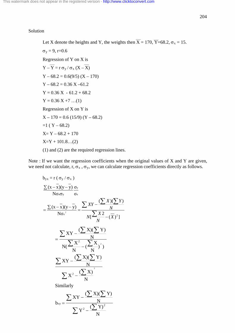
204

Solution

Let X denote the heights and Y, the weights then X = 170, Y=68.2, sx = 15.

sy = 9, r=0.6

Regression of Y on X is

Y – Y = r sy / sx (X – X)

Y – 68.2 = 0.6(9/5) (X – 170)

Y – 68.2 = 0.36 X –61.2

Y = 0.36 X - 61.2 + 68.2

Y = 0.36 X +7 …(1)

Regression of X on Y is

X – 170 = 0.6 (15/9) (Y – 68.2)

=1 ( Y – 68.2)

X= Y – 68.2 + 170

X=Y + 101.8…(2)

(1) and (2) are the required regression lines.

Note : If we want the regression coefficients when the original values of X and Y are given, we need not calculate, r, sx , sy, we can calculate regression coefficients directly as follows.

byx = r ( sy / sx )

])(2

[

))((

Nσ

)y)(yx(x

σ

σ

Nσ

)y)(yx(x

2x

x

y

yx

2

XN

XN

N

YXXY

-

-=

å --=

å --

å

å å ås

N

Y)(Y

N

Y)X)((XY

b

Similarly

N

)X(X

N

)YX)((XY

))N

X(

N

XN(

N

)YX)((XY

2

2

xy

2

2

2

2

åå

å å å

åå

å å å

åå

å å å

-

-=

-

-

-

-=



205

Examble 2. Find the regression equations from the following data The data relates the Number of air samples and So2 content of stack gas Table.24.6. Number of air samples and So2 content of stack gas

X 4 6 8 9 10 Y(µg/m3) 10 11 13 17 20

Solution Table.24.7.Calculation

X Y XY X2 Y2

4 10 40 16 100 6 11 66 36 121 8 13 104 64 169 9 17 153 81 289 10 20 200 100 400 37 71 563 297 1079

53.0

5

71 - 1079

5

(71)(37) - 563

bxy

N

)Y(Y

N

Y)X)((XY

bxy

N

)Y(Y

N

Y)X)((XY

.6.1

5

)37(297

5

)37)(71(563

N

)X(X

)N

Y)X)((XY

b

2

2

2

2

2

2

2

2

xy

==

-

-=

-

-=

=

-

-

-

-=

åå

å å å

åå

å å å

åå

å å å

2.145

71

4.75

37

==

==

y

x



206

The regression equation of Y on X is ( Y – Y ) = byx ( X – X) Y – 14.2 = 1.6 ( X – 7.4) Y = 1.6 X + 2.36

The regression equation of X on Y is (X – X) = bxy ( Y – Y) X – 7.4 = 0.53 ( Y – 14.2) X = 0.53 Y – 0.126

Self Check Exercise 4 1. In a study on the price of tiger skin and its demand in market the following results

were obtained. Average price (in Rs. Per kg) = 83 S.D. of prices (in Rs.) = 10 Average demands (in kg) = 1780 S.D. of prices (in kg.) = 37 Correlation coefficient between Price and demand = - 0.85 Estimate the average demand when price is 100 rupees and the average ruling price when demand is 2000 kg.

2. Given the regression equation to be 8 X + 15Y = 650 and 12 X + 10 Y = 600 estimate means of X and Y and also the correlation coefficient between them.

24.6. Let us sum up

In this lesson we have been about o The methods of predicting correlation between variables o The method of linear regression analysis o Properties of linear regression analysis.


· If the coefficient of correlation is +1. What is the significance of the study? · If there is a perfect negative correlation between two variables, what do you

understand? 24.8 Points for discussion ü Could you correlate the amount of Ca in water and the Ca in soil. Find the co-efficient

of correlation. ü Describe the method to formulate the lines of regression for the given set of values.


· For the first question you can very well calculate the co efficient of correlation. You have done similar sum in the lesson .You practice doing the sum. Otherwise do not proceed. If you have understood the concept you can give an example by yourself as follows:



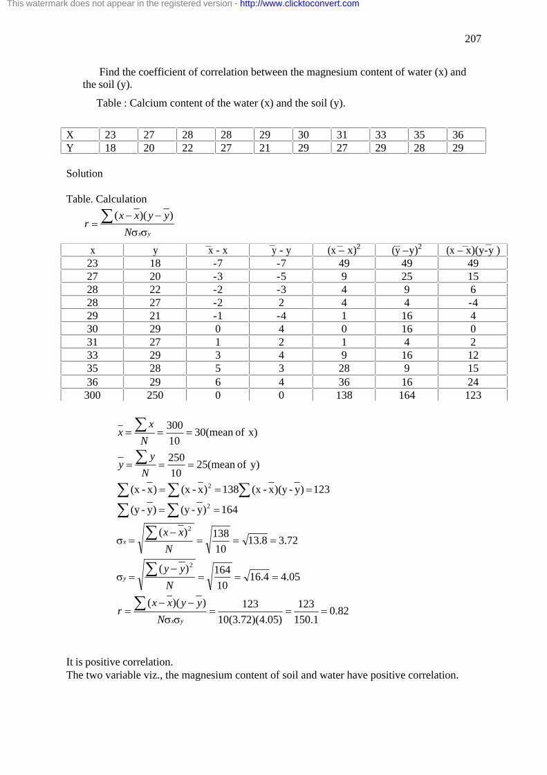
207

Find the coefficient of correlation between the magnesium content of water (x) and the soil (y).

Table : Calcium content of the water (x) and the soil (y).

X 23 27 28 28 29 30 31 33 35 36 Y 18 20 22 27 21 29 27 29 28 29 Solution Table. Calculation

It is positive correlation. The two variable viz., the magnesium content of soil and water have positive correlation.

x y x - x y - y (x – x)2 (y –y)2 (x – x)(y-y ) 23 18 -7 -7 49 49 49 27 20 -3 -5 9 25 15 28 22 -2 -3 4 9 6 28 27 -2 2 4 4 -4 29 21 -1 -4 1 16 4 30 29 0 4 0 16 0 31 27 1 2 1 4 2 33 29 3 4 9 16 12 35 28 5 3 28 9 15 36 29 6 4 36 16 24 300 250 0 0 138 164 123

yxN

yyxxr

ss

å --=

))((

82.01.150

123

)05.4)(72.3(10

123))((

05.44.1610

164)(

72.38.1310

138)(

164)y-(y)y-(y

123 )y-)(yx-(x138)x-(x)x-(x

y) of(mean 2510

250

x)of(mean 3010

300

2

2

2

2

===--

=

===-

=

===-

=

==

===

===

===

å

å

å

å ååå å

å

å

yx

y

x

N

yyxxr

N

yy

N

xx

N

yy

N

xx

ss

s

s



208

· For the second question explain the concept of regression lines and explain with an example. Be sure about the formulas. Example:The following data are given about the heights (in cms) and weights ( in

kgs) of 1000 wrestlers. Average height = 170 cm Average weight = 68.72 kg Standard deviation of heights = 15cms Standard deviation of weights = 9 kgs Coefficient of correlation between heights and weights = 0.6 Find the regression lines.

Solution

Let X denote the heights and Y, the weights then X = 170, Y=68.2, sx = 15.

sy = 9, r=0.6

Regression of Y on X is

Y – Y = r sy / sx (X – X)

Y – 68.2 = 0.6(9/5) (X – 170)

Y – 68.2 = 0.36 X –61.2

Y = 0.36 X - 61.2 + 68.2

Y = 0.36 X +7 …(1)

Regression of X on Y is

X – 170 = 0.6 (15/9) (Y – 68.2)

=1 ( Y – 68.2)

X= Y – 68.2 + 170

X=Y + 101.8…(2)

(1) and (2) are the required regression lines. 24.10 References 1. Statistical Methods – S. P. Gupta 2. Elements of Biostatistics – S Prasand 3. Introduction to statistics - R. P. Hoda 4. Biostatistics – P. K. Jasra and Gurdeep Raj 5. Genetics and biostatistics – N. T. Krishnan and M.S.M.S. Hussain 6. Statistical methods for biologists – S. Palanichamy and M. Manoharan 7. R. A. Fisher (1915). "Frequency distribution of the values of the correlation coefficient

in samples from an indefinitely large population". Biometrika 10: 507–521. 8. R. A. Fisher (1921). "On the probable error of a coefficient of correlation deduced from

a small sample". Metron.



209

9. K. Gayen (1951). "The frequency distribution of the product moment correlation coefficent in random samples of any size draw from non-normal universes". Biometrika 38: 219–247.

10. Cohen, J. (1988). Statistical power analysis for the behavioral sciences (2nd ed.) Hillsdale, NJ: Lawrence Erlbaum Associates. ISBN 0-8058-0283-5.

11. Anscombe, Francis J. (1973) Graphs in statistical analysis. American Statistician, 27, 17–21.

12. Cohen, J., Cohen P., West, S.G., & Aiken, L.S. (2003). Applied multiple regression/correlation analysis for the behavioral sciences. (2nd ed.) Hillsdale, NJ: Lawrence Erlbaum Associates

13. Draper, N.R. and Smith, H. Applied Regression Analysis Wiley Series in Probability and Statistics (1998)

14. Francis Galton. "Regression Towards Mediocrity in Hereditary Stature," Journal of the Anthropological Institute, 15:246-263 (1886). (Facsimile at: [1])

15. Robert S. Pindyck amd Daniel L. Rubinfeld (1998, 4h ed.). Econometric Models and Economic Forecasts,, ch. 1 (Intro, incl. appendices on Σ operators & derivation of parameter est.) & Appendix 4.3 (mult. regression in matrix form).

16. http://homepage.mac.com/nshoffner/nsh/CalcBookAll/Chapter%201/1functions.html



210

Lesson 25 TESTS OF HYPOTHESIS Contents


25.1. Introduction


25.3. Statistical inference

25.3.1. Estimation

25.3.2. Statistical hypothesis

25.3.3. Large Sample

25.3.4. Small Sample

25.4. Applications of the t-distribution

25.5. Chi-Square test (x2 test)

25.6. Analysis of Variance

25.6.1. One way classification

25.6.2. Two way classification

25.7. Let us sum up




25.11 References

25.0. Aims and objectives In this lesson we will learn about the testing of hypothesis. The t – test, Chi-square test and ANOVA will be discussed in detail. 25.1. Introduction

Statistics may be broadly divided into two categories called descriptive and inductive statistics. Descriptive statistics includes calculation and presentation of data. This inductive statistics or statistical inference is to make inference about a population based on information given. A portion selected from a population is called a sample and the process of selection is called sampling. The numbers of elements in a sample is called the sample size. The theory of sampling is a tool to get as much information as possible about the population from which the sample has been drawn. When sample descriptions are used to infer some information about the population, the subject is called inductive statistics or statistical interference.



211


If the nature of the population is known the sampling distribution can be obtained using the theory of probability. For example if the population is normal with mean µ and S.D. s, the sampling distribution of the sample mean x is also normal with mean m and S.D. s / n. 25.3. Statistical interference

The important branch of statistics, known as the statistical inference may be broadly classified into the following two headings.

i) Estimation ii) Testing hypothesis.


1. What is inductive statistics? ………………………………………………………………………………………………….. ………………………………………………………………………………………………….. ………………………………………………………………………………………………….. ………………………………………………………………………………………………….. ………………………………………………………………………………………………….. 25.3.1. Estimation

An estimation is a numerical value of the population parameter, whereas an estimator is a sample statistics used to estimate the population parameter, i.e. some features of the population in which an enquirer is interested may be completely unknown to him and he may wish to make a intelligent guess or scientific guess about this feature completely on the basis of a random sample from the population. Estimation is divided into two types: Point estimation and interval estimation.

Point estimation A particular value of a statistic, which is used to estimate a given parameter is known

as a point estimate of the parameter. For example a biologist takes a sample of 100 white mice and finds out their the average tail length If this figure is used to estimate as the average tail length for all the white mice in the region, it is referred to as a point estimate.

Interval Estimation An alternative procedure to point estimation is to give an interval within which the

parameter may be expected to lie with a specified degree of confidence. This is called interval estimation or confidence interval. Interval estimates indicate the precision or accuracy of an estimate and are therefore preferable to point estimates.



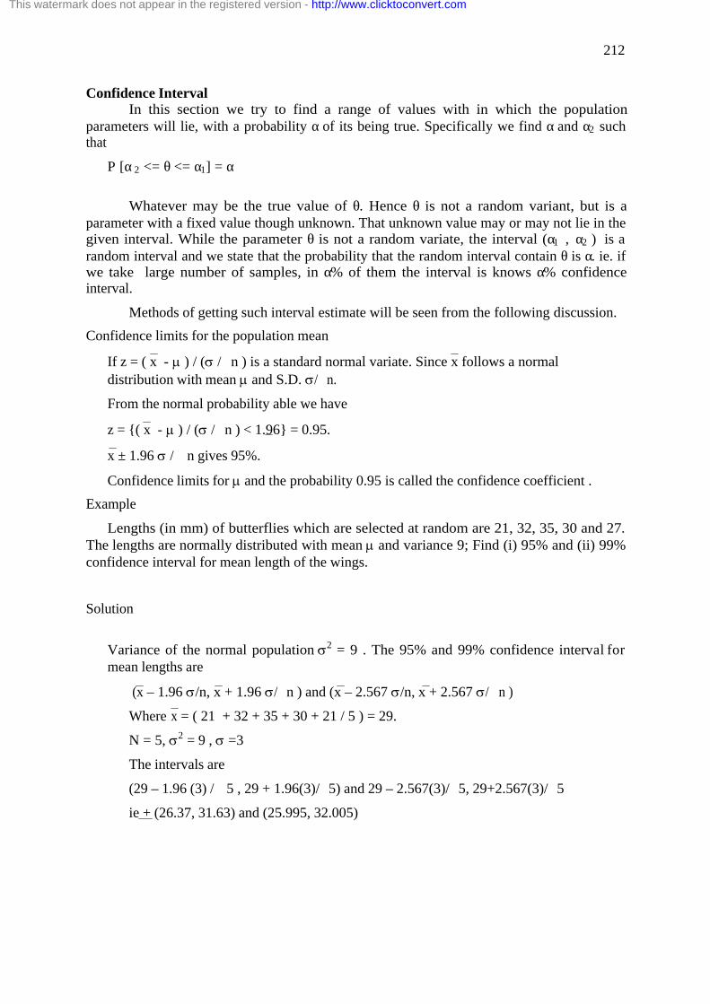
212

Confidence Interval In this section we try to find a range of values with in which the population

parameters will lie, with a probability α of its being true. Specifically we find α and α2 such that

P [α 2 <= θ <= α1] = α

Whatever may be the true value of θ. Hence θ is not a random variant, but is a parameter with a fixed value though unknown. That unknown value may or may not lie in the given interval. While the parameter θ is not a random variate, the interval (α1 , α2 ) is a random interval and we state that the probability that the random interval contain θ is α. ie. if we take large number of samples, in α% of them the interval is knows α% confidence interval.

Methods of getting such interval estimate will be seen from the following discussion.

Confidence limits for the population mean

If z = ( x - m ) / (s / n ) is a standard normal variate. Since x follows a normal distribution with mean m and S.D. s/ n.

From the normal probability able we have

z = {( x - m ) / (s / n ) < 1.96} = 0.95.

x ± 1.96 s / n gives 95%.

Confidence limits for m and the probability 0.95 is called the confidence coefficient .

Example

Lengths (in mm) of butterflies which are selected at random are 21, 32, 35, 30 and 27. The lengths are normally distributed with mean m and variance 9; Find (i) 95% and (ii) 99% confidence interval for mean length of the wings.

Solution

Variance of the normal population s2 = 9 . The 95% and 99% confidence interval for mean lengths are

(x – 1.96 s/n, x + 1.96 s/ n ) and (x – 2.567 s/n, x + 2.567 s/ n )

Where x = ( 21 + 32 + 35 + 30 + 21 / 5 ) = 29.

N = 5, s2 = 9 , s =3

The intervals are

(29 – 1.96 (3) / 5 , 29 + 1.96(3)/ 5) and 29 – 2.567(3)/ 5, 29+2.567(3)/ 5

ie + (26.37, 31.63) and (25.995, 32.005)



213

Tests of hypothesis In biology the results of experiments are usually not clear cut and therefore they need

statistical tests to support decisions between alternative hypothesis.

25.3.2. Statistical hypothesis.

A statistical hypothesis is a statement, which may or may not be true about the population. The hypothesis is denoted by H.

If the whole population could be examined, any hypothesis could be completely verified. But in the majority of cases only estimates of the parameter obtained from random samples are available and the hypothesis must be tested using these estimates. These tests are generally called tests of hypothesis or tests of significance. A statistical test is a decision taken after observing a random sample from the given population. The decision may be the acceptance or rejection of the hypothesis.It is thus based on the information contained in the sample, which may be consistent or inconsistent with the hypothesis.

Null and Alternative hypothesis A hypothesis is a statement about a population parameter. In testing of hypothesis

problem, we are faced with a pair of hypothesis such that one and only one of them are always true. One of this pair is called the null hypothesis and the other one the alternative hypothesis is represented as H1. For example, if the population mean is represented by m, we can set up our hypothesis as follows.

H0 : m < 20

H1 : m >20

The null hypothesis is called by this name because in many situations, acceptance of this null hypothesis would lead to null action. On the other hand rejecting the null hypothesis would lead to a change in existing status of the situations.

Type I and Type II errors.

As shown in table below. There can be two types of errors and for convenience each of these errors has been given a name.

Table.25.1. Types of errors in testing of hypothesis

Decision based on sample

Accept H0 (Reject H1) Reject H0 (accept H1)

H0 is true

H1 is false

Correct Wrong (Type I error)

States of Population

H0 is false

H1 is true

Wrong (Type II error)

Correct



214

If we wrongly reject H0 when in reality H0 is true the error is called a type I error. Similarly, when we wrongly accept H0 when H0 is false-the error is called a type II error.

The significance level In all tests of hypothesis, type I error is assumed to be more serious than type II error,

and so the probability of type I error needs to be explicitly controlled. This is done through specifying a significant level at which a test is conducted. The significance level therefore set a limit to the probability of type I error and test procedures are designed so as to get the lowest probability of type II error subject to the significance level.

The probability of type I error is usually represented by the symbol a and the probability of type I error is represented by b .

ie a = P (Type I error)

=P(Rejecting H0 when it is true)

The complement of this is

1-a= P (Accept H0 when it is true

This probability (1-a) corresponds to the concept of 100 (1-a) percent. Confidence interval similarly the probability of committing a type I error is denoted by b . Thus.

b=Pr(Type II error)

P (Accept H0 when it is false)

1- b = P (Reject H0 when it is false) This probability 1-b is known as the power of a statistical test.

The probabilities a and b are not independent of each other and also they are not independent of the sample size, n .When n is fixed and a decreases then b normally increases and vice versa. If n is increased it is possible for both a and b normally increases and vice versa. If n is increased it is possible for both a and b to decrease while testing hypothesis the aim is to reduce both type of errors. It is also more serious to accept a wrong hypothesis than to reject a correct one that is, consequently of type II error, are likely to be more serious than the consequences of type I error. Hence a compromise procedure to get a satisfactory test is to minimize more serious error after fixing up this less serious error. In practice the common levels of significance are 0.05 (5%) and 0.01 (1%) 5% level of significance implies that we are 95% confident

Degrees of freedom

Number of independent random observation is called the number of degrees of freedom. Each constraint in the random observations will reduce one degrees of freedom. That is, if n is the number of random Observations (sample size) and k is the number of independent constants then the number of degrees of freedom of a statistic (on sampling distribution) based on the information is (n-k).

Standard error (S.E) The standard deviation of the sampling distribution is called the standard error. For

example, X1, X 2, … are the means of all the samples drawn from the population. The standard deviation of all these means is the standard error of the mean. The formula for this is s/ n.



215

25.3.3. Large Samples If the sample size is greater than 30 , then those samples may be regarded as large

samples.

25.3.4. Small Samples (Sampling Variables) If the size of the sample is less than 30, it is regarded as small sample. For testing

such samples the method used is as below.

Student’s distribution Gosset and Sir William are the pioneers who contributed to the theory of small

samples. Gosset published his discovery in 1905 under the pen name “student” and it is popularly known as t-test or t-distribution or students distribution. It is used when the sample is in small size and the population standard deviation is unknown.

Under the assumption of a normally distributed population, the t-distribution has been derived mathematically i.e.

f(t) = c ( 1 + t2/v) – ( v + i ) / 2

Where

t= ( x -m / S ) n

C=constant required to make the area under the curve equal to unity

v= n-1 the number of degrees of freedom.


2 .Define degrees of freedom. ………………………………………………………………………………………………….. ………………………………………………………………………………………………….. ………………………………………………………………………………………………….. ………………………………………………………………………………………………….. …………………………………………………………………………………………………..

25.4. Application of the t-distribution

To Test the significance of the mean of a random sample

To find out whether mean of the sample drawn from a normal population deviates significantly from the hypothetical value, we use t-distribution. The formula is

t = (( x - m ) x n ) / S

Where x = mean of the sample

m = The actual or hypothetical value of the population

n = Number of observations

S = The standard deviation of the sample.



216

S = {X - X) 2 / n-1

If deviation are taken from actual mean

S = ( d2-(d)2x n ) / n-1

Where d = deviation from actual mean, the 95% fiducial limits of the population mean (m) are:

x ± s/ n x t 0.05

and 99% limits are

x ± s/ n x t 0.01

Example 1

The total hardness of 10 water samples of collected from bore wells of Gandhipuram, Coimbatore is as follows

148, 128, 147, 127, 150, 145, 124, 140, 142, 149

i) In the light of the data, discuss the suggestion that the average total hardness of the population is 150.

ii) Set 95% confidence interval for the total hardness of water of the area.

Solution

Let us the hypothesis that the total hardness of the area is 150.

Table.25.2. Calculation of t value

Total hardness

( x - x ) =(x-140)

(x – x)2

148

128

147

127

150

145

124

140

142

149

8

-12

7

-13

10

5

-16

0

2

9

64

144

49

169

100

25

256

0

4

81

x = 1400 (x-x)2 = 892



217

x= x / n = 1400/10 = 140

S = (x – x)2 / ( n-1) = 892/9 = 9.96.

t = ( x - m ) / S x n = [(140-150) / 9.96 ] x 10

= (10 x 3.16 ) / 9.96 = 3.17

Degree of freedom = 10-1=9 for 9 degree of freedom, the table value at 5% level of significance is 2.26.

As the calculated value of t is higher than table value, we can not accept the hypothesis. Thus, we can conclude that the Total hardness is not 150 mg/L

Example 2

A random sample of size 10 had a mean, x = 15.5 and a variance, S2 = 4. Test at the 5 percent level of significance that the mean of the population m = 15.

Solution Let us take the hypothesis that the mean of the population is 15.

t = [( x - m ) / S ] x n

= [(15.5 – 15) / 4 ] x 3.16

= 0.5/4 x 3.16 = 0.395.

g = 9 , t 0.05 = 2.26

Since the calculated value 0.395 is less than the table value, we can accept the hypothesis that the mean of the population is 15.

To test the significance of the difference between two sample means:

To test the significance of the difference between two sample means, the value of t. is calculated by applying the following formula.

t = ( x1 – x2 ) / S n1 x n2 / n1 + n2

Where x1 and x2 are the means of first and second samples respectively, n1, n2 is the number of items of the two samples, and S is the combined standard deviation.

The value of 2nn

)Ax(n-)Ax(n)A(x)A(xs

21

2222111

222

211

-+

----+-=

åå

Where A1 = Assumed mean of the first sample

A2 = Assumed mean of the second sample

Example



218

Two types of bacterial strains were used on 5 and 7 dyeing samples for reducing the dye content.

Table.25.3 Data on dye removal

Dye A - 10 12 13 11 14 -

Dye B 8 9 12 14 15 10 9

If the bias correction due to small is ignored, pooled estimate of the standard deviation can be obtained by

Is there a significant difference in the removal of the two dyes? If not, which dye is removed efficiently? (for γ = 10. t 0.05 = 2.228.)

Solution

Let us take the hypothesis that there is no significant difference in the removal of the two dyes. Applying t – test.

t = ( x1 - x2 ) / S (n1n2) / ( n1 + n2 )

Table.25.4. Calculation of t value

x1

(x1 – x1)

(x1 – x1)2 x2

(x2 – x2)

(x2 – x2)2

10

12

13

11

14

-2

0

+1

-1

+2

4

0

1

1

4

8

9

12

14

15

10

9

-3

-2

+1

+3

+4

-1

-2.

9

4

1

9

16

1

4

x1 = 60 ( x1 – x1)2 = 10 x2 = 77 (x2 – x2)2=44

However , it is advisable to take account If bias.

21

2211

nn

snsns

22

+

+=



219

X1 = X1 / n1 = 60/5 = 12.

X2 = X2 / n2 = 77/7 = 11

For , The calculated value of t is less than the table

value, the hypothesis is accepted. Hence, there is no significance in the removal of two dyes. To test the significance of an observed correlation co-efficient

When we want to test whether r is not significantly greater than zero, that is to say, if we are interested in testing the “null hypothesis” that the variables in the population are uncorrelated, the flowing formula is to be used

t = [ r / (1 – r2) ] x (n-2) here, t is based on (n-2) degree of freedom

Example

A random sample if 27 pairs of observations from a normal population gives a correlation coefficient c.f. 0.40 is it likely that the variables in the population are un correlated? Solution

Let us take the hypothesis that there is no significant difference in the sample correlation and correlation in the population. Applying t-test

t = [ r / (1 – r2) ] x (n-2) r = 0.40 n=27 t = [ 0.40 / (1 – (0.40)2) ] x (25)

2.22810,γ

102752nnγ

0.735

2.324

1.708

75

5x7

2.324

1112

nn

nn

s

xxt

.324.210

54

275

4410

2nn

)x(x)x(xs

05.0

21

21

2111

21

222

211

==

=-+=-+=

=

=+

-=

+=

-=

==

-+

+=

-+

-+-=

åå

t



220

= (0.40 / 0.84 ) x 5 = 2.38

For V = 25 t0.05 = 1.708. The calculated value of t is more than the table value. The hypothesis is rejected. Hence it is likely that the variables in the population are uncorrelated. Example 2

A random sample of 18 pairs of observation from a normal population gives a correlation co-efficient of 0.52 is it likely that the variables in the population are un-correlated. Solution

Let us take the hypothesis that the variables in the population are uncorrelated. Applying t-test T = r / (1 – r2) x (n-2) = (0.52 x 4) / (1-.27) = 2.08 / 03.85 = 2.4 Degree if freedom = 18 – 2 = 16 For V = 16 t0.05 = 2.12

Since the calculated value of t is greater than the table value, we cannot accept the hypothesis. Hence, we may conclude that variables in the population are correlated.

Self Check Exercise 3

1. 10 workers are selected at random from a large number of workers in a factory. The number of times they are affected by asthmatic complaint due to asbestos in a year are found to be 51 52 53 55 56 57 58 59 59 60 In the light of these data would it be appropriate to suggest that the mean of the number times they are affected is 58?

2. Sample of two different types of fishes were tested for length of life, due to water contamination with Hg and the following data were obtained.

Type I Type II Sample Size Sample Mean Sample S.D.

8 1234 hrs 36hrs

7 1136 hrs 40 hrs

In the difference in the means significance (Given that the significant value of t at 5% level of significance of 13 d.7 is 2.16.

25.5. χ2 Test



221

It is a general purpose test and as such, is highly useful in research. The test is based on events or frequencies. This test is applied to draw inferences regarding the hypothesis but not useful for estimation. The test can be used between the entire set of observed and expected frequencies. For every increase in the number of degree of freedom, a new χ2distribution is formed. It can be applied for large and independent observations..

If χ2 is zero, it means that the observed and expected frequencies completely

coincide. The greater the discrepancy between the observed and expected frequencies, the greater is the value of x2. The quantity of x2 is defined as

χ2 = E ((O – E)2 / E ) Where, O = Observed Frequencies E = Expected frequencies It the calculated value of χ2is greater than the table value of χ2 at certain level of

significance, usually 5% the difference between theory and observations is considered to be significant i.e., we reject the hypothesis. If the computed value of χ2 is less than the table value at a certain degree of level of significant this implies that the discrepancy between the observed and expected frequencies may be due to Fluctuations in simple sampling i.e. we shall accept the hypothesis. Example.1.

From the data given below about the treatment of 250 H2O samples containing chromium using low cost adsorbent and activated carbon. State whether low cost is adsorbent is superior to activated carbon.

Table.25.5.Water treatment data Treatment Favorable

Removal Unfavorable removal Total

Low Cost adsorbent 140 30 170 Activated Carbon 60 20 80 Total 200 50 250 Given for degree of freedom = 1 , Chi Square 5 percent = 3.84. Solution

Let us set the hypothesis that there is no significant difference between the low cost adsorbent and activated carbon treatment. On applying χ2 test.

Excepted frequency of (AB) = 200 x 170 / 250 = 136 The table of expected frequencies shall be as follows. Table.25.6.Expected frequencies

136 34 170 64 16 80 200 50 250



222

Table.25.7.Calculation

O E (O - E)2 (O - E)2 / E 140 60 30 20

136 64 34 16

16 16 16 16

0.118 0.250 0.471 1.000

[ (O-E)2 / E ] = 1.839

χ2 = [ ( O – E)2 / E ] = 1.839 γ = (r – 1) ( c – 1) = (2 – 1) (2 – 1) =1 γ = 1 , χ20.05 = 3.84

The calculated value of χ2 is less than the table value. The hypothesis is accepted. Hence there is no – significant difference between the low cost adsorbent and activated carbon treatment. Example 2 RBC’s count lac/mm3 and working in a factory was recorded as follows. Is there any significant relation between RBC’s count and Hb% ? Find it by Chi-square method. Table.25.8.RBC count and Hb % of workers.

H b % RBC’s Count

Above normal Below normal Total

Above normal Below normal

85 165

75 175

160 340

Total 250 250 500 Solution Make following two tables to obtain χ2 Table.25.9.Calculation

H b % RBC3 Count

Above normal Below normal Total

Above normal Below normal

O=85 E=(250x160)/500 = 80 O=165 E=(250x340)/500 = 170

O=75 E=(250x160)/500 = 80 O=175 E=(250x340)/500 = 170

160 340

Total 250 250 500 On the basis of above data following table is prepared.



223

Table.25.10.Calculation

O E (O - E) (O - E)2 (O - E)2 / E 85 165 75 175

80 170 80 170

85-80=5 165-170=-5 75-80=-5 175-170=5

25 25 25 25

25/80 = 0.31 25/170 = 0.15 25/80 = 0.31 25/170 = 0.15

[ (O-E)2 / E ] = 0.92 Here df = (2-1) x (2-1) = 1 Significance

At 5% significance level of table value of χ2at 1 df = 3.84, the calculated value comes to 0.92. It indicates that Hg% and RBC’s count are fully independent of each other. Self-Check Exercise 4

4. Do you think t test is important for testing the hypothesis? ………………………………………………………………………………………………….. ………………………………………………………………………………………………….. ………………………………………………………………………………………………….. ………………………………………………………………………………………………….. …………………………………………………………………………………………………..

25.6. Analysis of Variance In statistics, analysis of variance (ANOVA) is a collection of statistical models, and their associated procedures, in which the observed variance is partitioned into components due to different explanatory variables. The initial techniques of the analysis of variance were developed by the statistician and geneticist R. A. Fisher in the 1920s and 1930s, and is sometimes known as Fisher's ANOVA or Fisher's analysis of variance, due to the use of Fisher's F-distribution as part of the test of statistical significance.The systematic procedure for the analysis of variance has been devised by R.A.Fischer. Analysis of variance consists of classifying and cross-classifying statistical results and testing whether the means of specific classification differ significantly. It can provide us with meaningful comparisons of sample data which are classified according to two or more variables. 25.6.1. One way classification

In one way classification the data are classified according to only one criterion. That is, the arithmetic means of populations from which k samples were randomly drawn are equal to one another.

Steps involved in the analysis are:

1. The calculate x12, x2

2, x32, …etc.

2. Find out the sum of T = x1 + x2 + x3 +……etc. 3. Find out the correction Factor = T2 / N 4. Find out the total sum of square = x1

2 + x22 + x3

2 +……-T2/N.



224

5. Find out the sum of between sample called grand average (( x1)2/N) + (( x2)2/N) + (( x3)2/N) – T2/N

6. Find out the sum of within samples. Total sum if square – sum if square between sample

7. The specimen ANOVA table is given below. Table.25.11.Specimen ANOVA table

Source of Variation

Sum of Squares Degree of Freedom

Mean Square F

Between sample Within sample

…………. ………….

g1 = c –1 g2 = c –1

Sum if square / c-1 Sum if square /

n - c

M e a n s q u a r e between column M e a n s q u a r e within sample

Total …………. n-1 Example Certain vermicompost was used on four plots of land, A, B, C, & D. The output of crops in the beds of the plots A, B, C, & D. is given below. Table.25.12.Output of crops

A B C D 6 10 2 4 5

9 3 6 2 1

12 8 2 6 4

3 4 5 8 2

Find out whether the difference in the means of the production of crops of the

plots is significant or not. Table.25.12.Calculation

Sample I Sample II Sample III Sample IV x1 x1

2 x2 x22 x3 x3

3 x4 x44

6 10 2 4 5

36 100 4 16 25

9 3 6 2 1

81 9 36 4 1

12 8 2 6 4

144 64 4 36 16

3 4 5 8 2

9 16 25 64 4

x1=21 x12=181 x2=21 x2

2=131 x3=32 x32=264 x4=22 x4

2=118 Total sum of the items of various samples = x1 + x2 + x3 + x4

= 21 + 21 + 32+ 22 = 96.

Correction Factor = T2/N = (96)2/20 = 9216/20 = 460.8

Total sum of squares (TSS)= x12 + x2

2 + x32 +……-T2/N.



225

= 181 + 131 + 264 + 118 – 460.8

= 694 –460.8 = 233.2.

Sum of Square between sample(SSBS)

= (( x1)2/N) + (( x2)2/N) + (( x3)2/N) + (( x4)2/N) – T2/N

= ((212/5) + (212/5) + (322/5) – (222/5)) – 460.8

= ((441/4) + (441/4) + (1024/4) + (484)/4) – 460.8

= 2390–2304 = 86/5 = 17.2

5

Sum of Square within samples (SSWS)= Total sum of square (TSS)-(SSBS) Sum of squares between samples SSWS = 233.2 – 17.2 = 216 Now, we can prepare ANOVA Table. Table.25.13.ANOVA table

Source of Variance Sum of Square Degree of Freedom Mean Square Between Samples Within Samples

17.2 216

γ1= c-1=5 – 1 =4 γ2= n –c = 20 – 5 = 15

SSBS/ γ1=17.2/4=4.3 SSWS/ γ2=216/15=14.4

Total 233.2 19 F = Variance between sample / Variance within sample = 4.3/14.4 = 0.30

The table value of ‘F’ for γ1 = 4 and γ2 = 15 at 5% level of significance = 3.06 The calculated value of ‘F’ is 0.30 is less than the Table value, so, we can

conclude that the sample is “not significant”. 25.6.2. Two way Classification

In a two-way classification, the data are classified according to two different criteria. Here, the analysis of variance table takes the following form.

Table.25.13.Other ANOVA table

Source of Variation

Sum of squares

Degree of Freedom

Mean square F

Between columns Between rows Residual error

SSC SSR SSE

C-1 r-1 (C-1)(r-1)

MSC = SSC / C-1 MSR = SSR / R-1 MSE = SSE / (r-1)(c-1)

MSC/MSE MSR/MSE

Total SST n-1 SSC – Sum of Square between columns SSR – Sum if Square between rows SSE – Sum of Square due to error.



226

SST – Total sum of squares.

The sum of squares for the sources ‘Residual’ is obtained by subtracting from the

total sum of squares the sum of squares between columns and rows. i.e. SSE = SST – (SSC + SSR ) In two way classification ‘Residual’ is the measuring rod for testing significance.

It represents the magnitude of variance due to forces called “chance”. Self Check Exercise 5

1. The following table gives the Total suspended solids of 15 water samples in three different bore wells. Find out whether the average TSS in different bore wells shows significant difference.

A B C 21 20 26 20 19 27 32 16 23 15 15 30 19 25 34


In this lesson we have discussed about

i. The tests of significance ii. The t test

iii. The Chi square test iv. And the Analysis of Variance


· Test the significance of various hypotheses. · Its applicability would be well understood if you go through the study material.

25.9 Points for discussion ü Write in detail about the significance of χ2 test.


· You would rather start explaining about the test as follows: It is a general purpose test and as such, is highly useful in research. The test is based on events or frequencies. This test is applied to draw inferences regarding the hypothesis but not useful for estimation. The test can be used between the entire set of observed and expected frequencies. For every increase in the number of degree of freedom, a new χ2distribution is formed. It can be applied for large and independent observations..



227

If χ2 is zero, it means that the observed and expected frequencies completely coincide. The greater the discrepancy between the observed and expected frequencies, the greater is the value of χ2. The quantity of χ2 is defined as

χ2 = ((O – E)2 / E ) Where, O = Observed Frequencies E = Expected frequencies It the calculated value of χ2is greater than the table value of χ2 at certain level of

significance, usually 5% the difference between theory and observations is considered to be significant i.e., we reject the hypothesis. If the computed value of χ2 is less than the table value at a certain degree of level of significant this implies that the discrepancy between the observed and expected frequencies may be due to Fluctuations in simple sampling i.e. we shall accept the hypothesis.

25.11 References

1. Statistical Methods – S. P. Gupta 2. Elements of Biostatistics – S Prasand 3. Introduction to statistics - R. P. Hoda 4. Biostatistics – P. K. Jasra and Gurdeep Raj 5. Genetics and biostatistics – N. T. Krishnan and M.S.M.S. Hussain 6. Statistical methods for biologists – S. Palanichamy and M. Manoharan 7. Ferguson, George A., Takane, Yoshio. (2005). "Statistical Analysis in Psychology

and Education", Sixth Edition. Montréal, Quebec: McGraw-Hill Ryerson Limited. 8. King, Bruce M., Minium, Edward W. (2003). Statistical Reasoning in Psychology and

Education, Fourth Edition. Hoboken, New Jersey: John Wiley & Sons, Inc. ISBN 0-471-21187-7

9. Lindman, H. R. (1974). Analysis of variance in complex experimental designs. San Francisco: W. H. Freeman & Co.



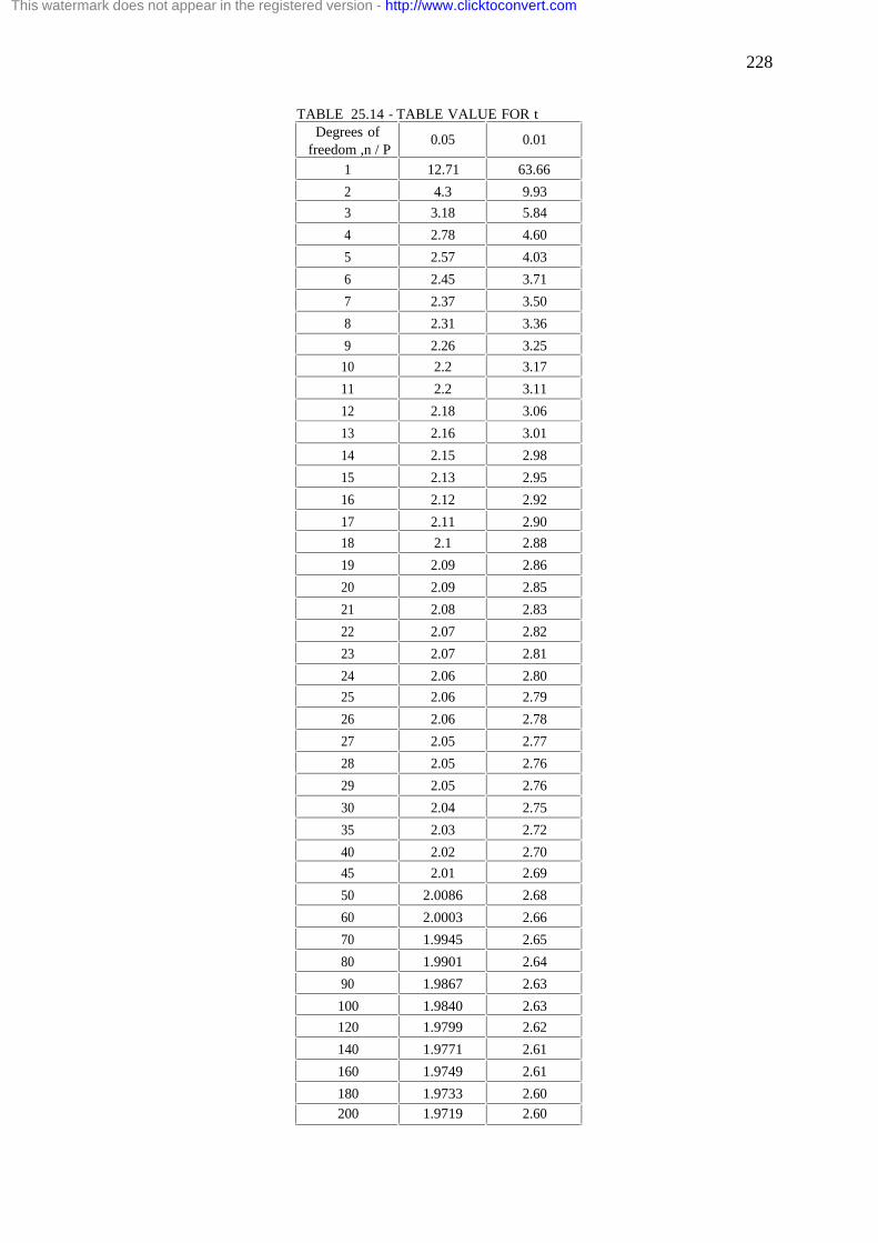
228

TABLE 25.14 - TABLE VALUE FOR t Degrees of

freedom ,n / P 0.05 0.01

1 12.71 63.66

2 4.3 9.93

3 3.18 5.84

4 2.78 4.60

5 2.57 4.03

6 2.45 3.71

7 2.37 3.50

8 2.31 3.36

9 2.26 3.25

10 2.2 3.17

11 2.2 3.11

12 2.18 3.06

13 2.16 3.01

14 2.15 2.98

15 2.13 2.95

16 2.12 2.92

17 2.11 2.90

18 2.1 2.88

19 2.09 2.86

20 2.09 2.85

21 2.08 2.83

22 2.07 2.82

23 2.07 2.81

24 2.06 2.80

25 2.06 2.79

26 2.06 2.78

27 2.05 2.77

28 2.05 2.76

29 2.05 2.76

30 2.04 2.75

35 2.03 2.72

40 2.02 2.70

45 2.01 2.69

50 2.0086 2.68

60 2.0003 2.66

70 1.9945 2.65

80 1.9901 2.64

90 1.9867 2.63

100 1.9840 2.63

120 1.9799 2.62

140 1.9771 2.61

160 1.9749 2.61

180 1.9733 2.60

200 1.9719 2.60



229

TABLE 25.15 - TABLE VALUE FOR χ2

Degrees of freedom ,γ / P 0.05 0.01

1 3.84 6.64

2 5.99 9.21

3 7.82 11.34

4 9.49 13.28

5 11.07 15.09

6 12.59 16.81

7 14.07 18.48

8 15.51 20.09

9 16.92 21.67

10 18.31 23.21

11 19.68 24.72

12 21.03 26.22

13 22.36 27.69

14 23.68 29.14

15 25.00 30.58

16 26.30 32.00

17 27.59 33.41

18 28.87 34.80

19 30.14 36.19

20 31.41 37.57

21 32.67 38.93

22 33.92 40.29

23 35.17 41.64

24 36.42 42.98

25 37.65 44.31

26 38.88 45.64

27 40.11 46.96

28 41.34 48.28

29 42.56 49.59

30 43.77 50.89

35 49.8 57.30

40 55.80 63.70

45 61.70 70.00

50 67.50 73.20

55 73.30 82.30

60 79.10 88.40

65 84.80 94.40

70 90.50 100.40

75 96.20 106.40

80 101.90 112.30

85 107.50 118.20

90 113.10 124.10

95 118.80 130.00

100 124.30 135.80



230

TABLE-III

Table value for F – 0.05%

γ1-numerator γ2

denominator 2 3 4 5 6 7 10 12 20 2 19.00 19.16 19.25 19.30 19.33 19.35 19.40 19.41 19.45 3 9.55 9.28 9.12 9.01 8.94 8.88 8.78 8.74 8.66 4 6.94 6.59 6.39 6.26 6.16 6.09 5.96 5.91 5.80 5 5.79 5.41 5.19 5.05 4.95 4.88 4.74 4.68 4.56 6 5.14 4.76 4.53 4.39 4.28 4.21 4.06 4.00 3.87 7 4.74 4.35 4.12 3.97 3.87 3.79 3.63 3.57 3.44 8 4.46 4.07 3.84 3.69 3.50 3.50 3.34 3.28 3.15 9 4.26 3.86 3.63 3.48 3.37 3.29 3.13 3.07 2.93 10 4.10 3.71 3.48 3.33 3.22 3.14 2.97 2.91 2.77 11 3.98 3.59 3.36 3.20 3.09 3.01 2.86 2.79 2.65 12 3.88 3.49 3.26 3.11 3.00 2.92 2.76 2.69 2.54 13 3.81 3.41 3.18 3.02 2.92 2.84 2.67 2.60 2.46 14 3.74 3.34 3.11 2.96 2.85 2.77 2.60 2.53 2.39 15 3.68 3.26 3.06 2.90 2.79 2.70 2.55 2.48 2.33 20 3.49 3.10 2.87 2.71 2.60 2.52 2.35 2.28 2.12 30 3.32 2.92 2.69 2.53 2.42 2.34 2.16 2.09 1.93



m.sc., environmental sciences …...17.2 principle 17.2.1 turbidimetry 17.3 instrumentation. 17.4...

Documents