msc thesis - computer engineering publications...
TRANSCRIPT

Computer EngineeringMekelweg 4,
2628 CD DelftThe Netherlands
http://ce.et.tudelft.nl/
2006
MSc THESIS
FPGA based accelerator for real-time skinsegmentation
Bart de Ruijsscher
Abstract
Faculty of Electrical Engineering, Mathematics and Computer Science
CE-MS-2006-08
Many real-time image processing applications are confronted withperformance limitations when implemented in software. The skinsegmentation algorithm utilized in the hand gesture recognition sys-tem as developed by the ICT department of Delft University ofTechnology presents an example of such an application. This the-sis project proposes the design of an FPGA based accelerator whichalleviates the host PC’s computational power required for real-timeskin segmentation. The communication between the host PC andthe accelerator is based on direct ethernet network connection, mak-ing the proposed accelerator highly portable with a wide range ofhost PC’s (both desktops and laptops). Moreover, the proposedframework is not limited only to the implemented skin segmentationalgorithm since the same architecture can be reused for accelerationof other image processing operations. We show that our design uti-lizes no more than 88% of the resources available within the targetedXC2VP30 device. In addition, our solution accelerates the skin seg-mentation algorithm by a factor of 1.43 compared to its softwareimplementation.


FPGA based accelerator for real-time skinsegmentation
a flexible gesture recognition system accelerator
THESIS
submitted in partial fulfillment of therequirements for the degree of
MASTER OF SCIENCE
in
COMPUTER ENGINEERING
by
Bart de Ruijsscherborn in Oostburg, the Netherlands
Computer EngineeringDepartment of Electrical EngineeringFaculty of Electrical Engineering, Mathematics and Computer ScienceDelft University of Technology


FPGA based accelerator for real-time skinsegmentation
by Bart de Ruijsscher
Abstract
Many real-time image processing applications are confronted with performance limitationswhen implemented in software. The skin segmentation algorithm utilized in the handgesture recognition system as developed by the ICT department of Delft University of
Technology presents an example of such an application. This thesis project proposes the designof an FPGA based accelerator which alleviates the host PC’s computational power required forreal-time skin segmentation. The communication between the host PC and the accelerator isbased on direct ethernet network connection, making the proposed accelerator highly portablewith a wide range of host PC’s (both desktops and laptops). Moreover, the proposed frameworkis not limited only to the implemented skin segmentation algorithm since the same architecturecan be reused for acceleration of other image processing operations. We show that our designutilizes no more than 88% of the resources available within the targeted XC2VP30 device. Inaddition, our solution accelerates the skin segmentation algorithm by a factor of 1.43 comparedto its software implementation.
Laboratory : Computer EngineeringCodenumber : CE-MS-2006-08
Committee Members :
Advisor: Georgi Gaydadjiev, CE, TU Delft
Advisor: Jeroen Lichtenauer, ICT, TU Delft
Chairperson: Stamatis Vassiliadis, CE, TU Delft
Member: Emile Hendriks, ICT, TU Delft
i

ii

iii

iv

Contents
List of Figures x
List of Tables xi
Acknowledgements xiii
1 Introduction 11.1 Hand gesture recognition . . . . . . . . . . . . . . . . . . . . . . . . . . . 11.2 Problem statement . . . . . . . . . . . . . . . . . . . . . . . . . . . . . . . 11.3 Objective and plan of approach . . . . . . . . . . . . . . . . . . . . . . . . 21.4 Chapter overview . . . . . . . . . . . . . . . . . . . . . . . . . . . . . . . . 2
2 Related work 52.1 Real-time skin segmentation . . . . . . . . . . . . . . . . . . . . . . . . . . 52.2 FPGA based acceleration of real-time image processing operations . . . . 62.3 Conclusion . . . . . . . . . . . . . . . . . . . . . . . . . . . . . . . . . . . 7
3 Image processing operations 93.1 Introduction . . . . . . . . . . . . . . . . . . . . . . . . . . . . . . . . . . . 93.2 Convolution . . . . . . . . . . . . . . . . . . . . . . . . . . . . . . . . . . . 9
3.2.1 Mean filter . . . . . . . . . . . . . . . . . . . . . . . . . . . . . . . 113.2.2 Gaussian smoothing filter . . . . . . . . . . . . . . . . . . . . . . . 113.2.3 Algorithmic representation of the convolution operation . . . . . . 12
3.3 Color space conversion . . . . . . . . . . . . . . . . . . . . . . . . . . . . . 133.4 Erosion and dilation . . . . . . . . . . . . . . . . . . . . . . . . . . . . . . 143.5 Local count and absolute difference . . . . . . . . . . . . . . . . . . . . . . 153.6 Summary . . . . . . . . . . . . . . . . . . . . . . . . . . . . . . . . . . . . 15
4 Implementation considerations 174.1 Exploiting Parallelism . . . . . . . . . . . . . . . . . . . . . . . . . . . . . 17
4.1.1 Instruction level parallelism . . . . . . . . . . . . . . . . . . . . . . 174.1.2 Task level parallelism . . . . . . . . . . . . . . . . . . . . . . . . . 18
4.2 Flexibility . . . . . . . . . . . . . . . . . . . . . . . . . . . . . . . . . . . . 194.3 Implementation platforms . . . . . . . . . . . . . . . . . . . . . . . . . . . 19
4.3.1 General purpose processor . . . . . . . . . . . . . . . . . . . . . . . 194.3.2 Digital signal processor . . . . . . . . . . . . . . . . . . . . . . . . 204.3.3 Application specific IC . . . . . . . . . . . . . . . . . . . . . . . . . 204.3.4 Programmable hardware . . . . . . . . . . . . . . . . . . . . . . . . 21
4.4 Conclusion . . . . . . . . . . . . . . . . . . . . . . . . . . . . . . . . . . . 21
v

5 Architecture design 235.1 Architecture . . . . . . . . . . . . . . . . . . . . . . . . . . . . . . . . . . . 23
5.1.1 Criteria for architecture design . . . . . . . . . . . . . . . . . . . . 235.1.2 System architecture . . . . . . . . . . . . . . . . . . . . . . . . . . 245.1.3 Accelerator architecture . . . . . . . . . . . . . . . . . . . . . . . . 255.1.4 Pixel Processing Pipeline subsystem architecture . . . . . . . . . . 27
5.2 Implementation constraints . . . . . . . . . . . . . . . . . . . . . . . . . . 285.2.1 Network bandwidth . . . . . . . . . . . . . . . . . . . . . . . . . . 285.2.2 Accelerator throughput . . . . . . . . . . . . . . . . . . . . . . . . 305.2.3 Pixel Processing Pipeline throughput . . . . . . . . . . . . . . . . . 31
5.3 Conclusion . . . . . . . . . . . . . . . . . . . . . . . . . . . . . . . . . . . 31
6 Implementation 336.1 Processor functionality . . . . . . . . . . . . . . . . . . . . . . . . . . . . . 33
6.1.1 Network protocol selection . . . . . . . . . . . . . . . . . . . . . . . 336.1.2 Interrupt handling . . . . . . . . . . . . . . . . . . . . . . . . . . . 34
6.2 Pixel Processing Pipeline . . . . . . . . . . . . . . . . . . . . . . . . . . . 356.2.1 Pipeline implementation . . . . . . . . . . . . . . . . . . . . . . . . 356.2.2 Pipeline protocol . . . . . . . . . . . . . . . . . . . . . . . . . . . . 366.2.3 Color space conversion . . . . . . . . . . . . . . . . . . . . . . . . . 386.2.4 Neighborhood implementation . . . . . . . . . . . . . . . . . . . . 386.2.5 Binary erosion, dilation and closing . . . . . . . . . . . . . . . . . . 416.2.6 Convolution filter . . . . . . . . . . . . . . . . . . . . . . . . . . . . 416.2.7 Local count . . . . . . . . . . . . . . . . . . . . . . . . . . . . . . . 426.2.8 Remaining operations . . . . . . . . . . . . . . . . . . . . . . . . . 436.2.9 Implementation results . . . . . . . . . . . . . . . . . . . . . . . . . 44
6.3 Summary . . . . . . . . . . . . . . . . . . . . . . . . . . . . . . . . . . . . 44
7 System verification and evaluation 457.1 Image processing components . . . . . . . . . . . . . . . . . . . . . . . . . 45
7.1.1 Color space conversion . . . . . . . . . . . . . . . . . . . . . . . . . 457.1.2 Binary dilation, erosion and closing . . . . . . . . . . . . . . . . . . 467.1.3 Uniform filter . . . . . . . . . . . . . . . . . . . . . . . . . . . . . . 477.1.4 Local count . . . . . . . . . . . . . . . . . . . . . . . . . . . . . . . 497.1.5 Remaining operations . . . . . . . . . . . . . . . . . . . . . . . . . 49
7.2 Pixel Processing Pipeline . . . . . . . . . . . . . . . . . . . . . . . . . . . 517.3 Integral system performance evaluation . . . . . . . . . . . . . . . . . . . 527.4 Conclusion . . . . . . . . . . . . . . . . . . . . . . . . . . . . . . . . . . . 53
8 Conclusions and Future Work 558.1 Conclusions . . . . . . . . . . . . . . . . . . . . . . . . . . . . . . . . . . . 558.2 Future work . . . . . . . . . . . . . . . . . . . . . . . . . . . . . . . . . . . 55
Bibliography 59
vi
A Skin segmentation algorithm 61A.1 Change detection . . . . . . . . . . . . . . . . . . . . . . . . . . . . . . . . 61A.2 Skin segmentation . . . . . . . . . . . . . . . . . . . . . . . . . . . . . . . 61
B PPP communication packets 63B.1 Ethernet packet header structure . . . . . . . . . . . . . . . . . . . . . . . 63B.2 Pixel packet structure . . . . . . . . . . . . . . . . . . . . . . . . . . . . . 64B.3 Configuration packet structure . . . . . . . . . . . . . . . . . . . . . . . . 65
C PPP slave registers 67
D Implementation data 69
E Design files overview 79E.1 Accelerator project . . . . . . . . . . . . . . . . . . . . . . . . . . . . . . . 79E.2 Pipeline components . . . . . . . . . . . . . . . . . . . . . . . . . . . . . . 79E.3 Verification software . . . . . . . . . . . . . . . . . . . . . . . . . . . . . . 79E.4 Demonstration software . . . . . . . . . . . . . . . . . . . . . . . . . . . . 79E.5 Miscellaneous . . . . . . . . . . . . . . . . . . . . . . . . . . . . . . . . . . 82
vii

viii

List of Figures
1.1 project overview . . . . . . . . . . . . . . . . . . . . . . . . . . . . . . . . 31.2 project black box representation . . . . . . . . . . . . . . . . . . . . . . . 3
3.1 image convolution process . . . . . . . . . . . . . . . . . . . . . . . . . . . 103.2 5x5 mean filter kernel centered around (0,0) . . . . . . . . . . . . . . . . . 113.3 5x5 gaussian filter kernel with σ = 2 centered around (0,0) . . . . . . . . . 123.4 application of mean filter (middle) and gaussian filter (right) . . . . . . . 123.5 application of a dilation (b), erosion (c), opening (d) and closing (e) op-
eration . . . . . . . . . . . . . . . . . . . . . . . . . . . . . . . . . . . . . . 16
5.1 system architecture . . . . . . . . . . . . . . . . . . . . . . . . . . . . . . . 265.2 example pixel packet flow . . . . . . . . . . . . . . . . . . . . . . . . . . . 275.3 pixel processing pipeline architecture . . . . . . . . . . . . . . . . . . . . . 29
6.1 PPP implementation diagram . . . . . . . . . . . . . . . . . . . . . . . . . 366.2 pipeline protocol state diagram . . . . . . . . . . . . . . . . . . . . . . . . 376.3 color space conversion block diagram . . . . . . . . . . . . . . . . . . . . . 396.4 kernel scanning process . . . . . . . . . . . . . . . . . . . . . . . . . . . . 396.5 general structure of a 5x5 neighborhood operation . . . . . . . . . . . . . 406.6 (uniform) filter kernel implementation . . . . . . . . . . . . . . . . . . . . 426.7 local count filter kernel implementation . . . . . . . . . . . . . . . . . . . 43
7.1 color space conversion results; original (a), software output (b), hardwaresimulation output (c) and difference between software and hardware (d) . 46
7.2 binary dilation results; original (a), software output (b), hardware simu-lation output (c) and difference between software and hardware (d) . . . . 47
7.3 binary erosion results; original (a), software output (b), hardware simula-tion output (c) and difference between software and hardware (d) . . . . . 48
7.4 binary closing results; original (a), software output (b), hardware simula-tion output (c) and difference between software and hardware (d) . . . . . 48
7.5 uniform filter results; original (a), software output (b), hardware simula-tion output (c) and difference between software and hardware (d) . . . . . 49
7.6 local count results; original (a), software output (b), hardware simulationoutput (c) and difference between software and hardware (d) . . . . . . . 50
7.7 threshold results; original (a), software output (b), hardware simulationoutput (c) and difference between software and hardware (d) . . . . . . . 50
7.8 pixel processing pipeline skin segmentation results; original (a), softwareoutput (b), hardware simulation output (c) and difference between soft-ware and hardware (d) . . . . . . . . . . . . . . . . . . . . . . . . . . . . . 51
7.9 Software algorithm performance . . . . . . . . . . . . . . . . . . . . . . . . 527.10 Hardware implementation performance . . . . . . . . . . . . . . . . . . . . 53
A.1 skin segmentation algorithm . . . . . . . . . . . . . . . . . . . . . . . . . 62
ix

B.1 common ethernet packet header structure . . . . . . . . . . . . . . . . . . 63B.2 pixel packet header structure . . . . . . . . . . . . . . . . . . . . . . . . . 64B.3 configuration packet header structure . . . . . . . . . . . . . . . . . . . . . 65
C.1 PPP slave register organization . . . . . . . . . . . . . . . . . . . . . . . . 67
x

List of Tables
6.1 XC2VP30 utilization summary . . . . . . . . . . . . . . . . . . . . . . . . 44
B.1 Input pixel format . . . . . . . . . . . . . . . . . . . . . . . . . . . . . . . 64B.2 Output pixel format . . . . . . . . . . . . . . . . . . . . . . . . . . . . . . 64
C.1 PPP Parameter Descriptions . . . . . . . . . . . . . . . . . . . . . . . . . 68
D.1 implementation metrics for accelerator system . . . . . . . . . . . . . . . . 69D.2 implementation metrics for pixel processing pipeline . . . . . . . . . . . . 70D.3 timing and implementation metrics for 7x7 local count component . . . . 71D.4 timing and implementation metrics for absolute difference component . . 72D.5 timing and implementation metrics for binary closing component . . . . . 72D.6 timing and implementation metrics for 5x5 uniform filter component . . . 73D.7 timing and implementation metrics for color space conversion component 73D.8 timing and implementation metrics for erosion/dilation component . . . . 74D.9 timing and implementation metrics for 24-bit signed adder component . . 74D.10 timing and implementation metrics for 19-bit unsigned divider component 75D.11 timing and implementation metrics for 16-bit signed multiplier component 75D.12 timing and implementation metrics for 32-bit pipeline register component 76D.13 timing and implementation metrics for 32-bit pipeline register component 76D.14 timing and implementation metrics for 1-bit delaying pipeline register
component . . . . . . . . . . . . . . . . . . . . . . . . . . . . . . . . . . . 77D.15 timing and implementation metrics for 16-bit delaying pipeline register
component . . . . . . . . . . . . . . . . . . . . . . . . . . . . . . . . . . . 77
E.1 overview of important accelerator project directories and files . . . . . . . 80E.2 overview of important accelerator project directories and files . . . . . . . 81
xi

xii

Acknowledgements
It was a great pleasure performing my thesis project at both the Computer Engineeringlaboratory and the ICT Group of Delft University of Technology. I am grateful thatEmile Hendriks initially provided me with this challenging assignment. I would liketo thank my advisors Georgi Gaydadjiev and Jeroen Lichtenauer for their professionalassistance and guidance throughout this project. Additionally, they spent long hoursduring their spare time critically reviewing my paper and report. I really appreciatethat.
Furthermore, the support of our Computer Engineering ”in-house” system adminis-trator Bert Meijs was much appreciated. All the software reinstalls, updates and addi-tions did not seem to tire him at all.
I would also like to extend my gratitude to my family for providing all the precondi-tions necessary to complete my studies. Without them, it would not have been possibleat all. In particular, I would like to thank Manon for providing unconditional supportand interest in my work.
Bart de RuijsscherDelft, The NetherlandsJune 19, 2006
xiii

xiv

Introduction 11.1 Hand gesture recognition
Human-computer interaction (HCI) is a discipline involved with the design, implementa-tion and evaluation of interactive computer systems which provide the user with naturaland efficient means for interaction. One of the known human communication modes isusing hand gestures. Systems capable of recognizing gestures are envisioned to providemore natural user interaction compared to systems relying only on keyboard and/ormouse user input. Application domains for hand gesture recognition include input andcontrol of user applications and games, interactive training of sign languages and behav-ior monitoring.
1.2 Problem statement
The Mediamatics department, part of the Electrical Engineering Mathematics and Com-puter Science faculty of Delft University of Technology, is currently developing a gesturerecognition system based on images captured by a digital video camera. The currentsystem is implemented in software and is unable to achieve the frame processing rateof 25 frames per second as is required for accurate hand gesture recognition. The pri-mary cause for this can be attributed to the skin segmentation algorithm computationaloverhead employed in the gesture recognition system. Currently, the system works withan image resolution of 160x120 pixels at a frame rate of 25 images per second. It isdesirable to improve the image resolution up to 640x480 pixels at the same frame rate.The higher resolution is desirable since it will make it possible to determine the shapeof a human hand, to perform better tracking of features and to have more freedom ofmovement for the user. This allows larger variations in distance between the user andthe camera. Furthermore, a higher resolution would allow the use of better methods ofgesture recognition since more details (such as seperate fingers) will be available.
Since the skin segmentation algorithm [22] is still under development, the definitiveversion has not yet been established. Consequently, in the future new operations might beincluded and some currently implemented operations might be excluded in the followingversions of the algorithm.
The main problem statement which presents the basic motivation for this thesisproject can therefore be formulated as follows:
How can the implementation of the existing skin segmentation algorithm be acceler-ated such that the gesture recognition system is able to operate at a video frame rate of25 frames per second and a resolution of 640x480 pixels? Furthermore, how can thisimplementation be achieved while providing the flexibility to support new versions of thealgorithm in the future?
1

2 CHAPTER 1. INTRODUCTION
1.3 Objective and plan of approach
The objective of this thesis project is to accelerate the skin segmentation algorithm inorder to meet the real-time requirements of the gesture recognition system at the desiredimage resolution and frame rate. A proof of concept has to be developed to demonstratethe operation of the proposed system. Figure 1.1 shows the conceptual representation ofthis thesis project. The PC captures images from a digital camera and sends these to theaccelerator. The accelerator processes the images as required by the skin segmentationalgorithm [22] and returns both a skin segmented image and an absolute differenceimage. High level applications can use the accelerator output for further processing. Forexample, a hand gesture recognition application may analyze the accelerator output tointerpret hand gestures. The interpretation may result in application specific feedbacksuch as character movement in a game or sign matching in a sign language trainingapplication.
A contextual black-box representation of the accelerator is depicted in figure 1.2. Thefigure shows that a stream of RGB images constitutes the input to the accelerator. Theoutput consists of both an absolute difference image stream and a skin segmented imagestream. The absolute difference image is used for change detection between subsequentframes, the skin segmented output is used for hand gesture recognition.
The plan of approach consists of the following phases:
• Literature study, both on hand gesture recognition and real-time image processingrelated systems;
• Selection of a suitable implementation platform;
• Architectural exploration and development of suitable processing architecture;
• Implementation, testing and performance evaluation of the architecture and itscomponents;
• Development of a demonstrator.
1.4 Chapter overview
The remainder of this document is organized as follows. Chapter 2 presents an overviewof previously reported work related to this project. Chapter 3 provides a descriptionof the image processing operations currently used in the skin segmentation algorithm.Chapter 4 discusses aspects important to the implementation of the accelerator andconcludes with a motivated choice for a suitable implementation platform. Chapter 5discusses the accelerator architecture and chapter 6 provides a detailed discussion on theimplementation of this architecture and its components. Chapter 7 provides the systemevaluation, chapter 8 then concludes with a summary of this project.

1.4. CHAPTER OVERVIEW 3
`
640x480, 25 fps
USB
uncompressed bitmap images
640x480, 25 fps
processed bitmap images
640x480, 25 fps
(+ additional information,
depending on the actual
implementation)
Accelerator
[to be developed]
user
skin
segmented
output
Programming and
communication interface
(API)
Application
application
specific
feedback
Figure 1.1: project overview
Skin segmentation
algorithm accelerator
RGB image sequence from webcam
skin
segmented
image
sequence
absolute
difference
image
sequence
Figure 1.2: project black box representation

4 CHAPTER 1. INTRODUCTION

Related work 2This chapter discusses previous related work. First, a short overview of real-time skinsegmentation methods is discussed. Then, an overview of known Field ProgrammableGate Array (FPGA) based solutions for accelerating real-time image processing opera-tions is presented.
2.1 Real-time skin segmentation
Many computer vision based methods for hand gesture recognition or skin color trackinghave previously been proposed in the literature. An interesting method for trackingmultiple skin colored objects proposed in [2], shows that it is possible to achieve real-timeperformance of the proposed algorithm. This skin segmentation algorithm is based ontransforming the 3D color representation (YUV) of input images to a 2D representation(UV) and calculating the probability of each pixel being a skin color. The reference forthis calculation is determined by a set of training images which has to be constructedmanually. The skin regions of the image are then grown into blobs1 which can be trackedthrough time. The disadvantage is the requirement of manual composition of the trainingset.
The discussion of a different approach proposed in [18] also claims to provide real-timeperformance of the skin segmentation algorithm. This work however lacks informationon the computational complexity of the algorithm, the video resolution and the framerate utilized. The method uses a look-up table of skin colors based on a predefinedtraining set. During run-time the skin segmentation is performed on a low resolutioninput image. One disadvantage of this method is the low resolution input image used forskin segmentation. Such reduced resolution prevents detection of details such as fingersand hand tilt.
To reduce the computational complexity of hand gesture recognition, several re-searchers have proposed alternative methods for hand tracking. For example, [19] pro-poses a method based on ”flocks of features” to track skin colored objects. The methodcalculates feature points within the hand area of an image and tracks these points overtime. The advantage of calculating a limited amount of feature points is the reductionof the computational complexity compared to calculations involving the complete inputimage. The disadvantage is the inability to precisely determine hand shape, tilt andfinger positions.
A different approach as mentioned in [1] is based on histogram segmentation. Themethod relies on dividing the image into small regions. For each region a histogramis calculated and matched with a training set. The advantage of this algorithm is a
1Blobs are solid circle or elliptical shaped object which represent a simplification of the object con-sidered.
5
6 CHAPTER 2. RELATED WORK
reduction of computational complexity but this particular algorithm lacks the ability totrack multiple objects in a single image.
The method utilized in this project is based on the algorithm as proposed in [22]which is currently under development at the ICT department of Delft University ofTechnology. It provides better results compared to other models [22] without requiringcolor calibration of the camera.
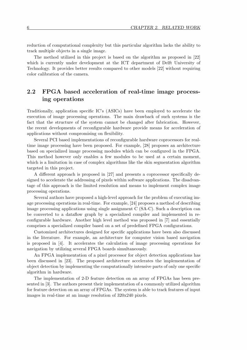
2.2 FPGA based acceleration of real-time image process-ing operations
Traditionally, application specific IC’s (ASICs) have been employed to accelerate theexecution of image processing operations. The main drawback of such systems is thefact that the structure of the system cannot be changed after fabrication. However,the recent developments of reconfigurable hardware provide means for acceleration ofapplications without compromising on flexibility.
Several PCI based implementations of reconfigurable hardware coprocessors for real-time image processing have been proposed. For example, [28] proposes an architecturebased on specialized image processing modules which can be configured in the FPGA.This method however only enables a few modules to be used at a certain moment,which is a limitation in case of complex algorithms like the skin segmentation algorithmtargeted in this project.
A different approach is proposed in [27] and presents a coprocessor specifically de-signed to accelerate the addressing of pixels within software applications. The disadvan-tage of this approach is the limited resolution and means to implement complex imageprocessing operations.
Several authors have proposed a high-level approach for the problem of executing im-age processing operations in real-time. For example, [24] proposes a method of describingimage processing applications using single assignment C (SA-C). Such a description canbe converted to a dataflow graph by a specialized compiler and implemented in re-configurable hardware. Another high level method was proposed in [7] and essentiallycomprises a specialized compiler based on a set of predefined FPGA configurations.
Customized architectures designed for specific applications have been also discussedin the literature. For example, an architecture for computer vision based navigationis proposed in [4]. It accelerates the calculation of image processing operations fornavigation by utilizing several FPGA boards simultaneously.
An FPGA implementation of a pixel processor for object detection applications hasbeen discussed in [23]. The proposed architecture accelerates the implementation ofobject detection by implementing the computationally intensive parts of only one specificalgorithm in hardware.
The implementation of 2-D feature detection on an array of FPGAs has been pre-sented in [3]. The authors present their implementation of a commonly utilized algorithmfor feature detection on an array of FPGAs. The system is able to track features of inputimages in real-time at an image resolution of 320x240 pixels.

2.3. CONCLUSION 7
2.3 Conclusion
The discussion in this chapter shows that previous work related to reconfigurable hard-ware acceleration of image processing operations has been proven successful. The maindisadvantage of the considered proposals is the PCI interface being employed. This limitsthe practical application of such accelerators to desktop systems only.
The high level approaches for describing image processing operations for reconfig-urable hardware may provide interesting alternatives to low level approaches. At thismoment however, the methods lack the possibility to implement complex algorithmsconsisting of multiple operations.
Taking into account the above mentioned aspects, we can summarize the requirementsfor our accelerator for real-time skin segmentation as follows:
1. Acceleration of the skin segmentation algorithm using a commonly available PCinterface, available on both desktop and laptop systems;
2. Flexible architecture of the accelerator which allows the implementation of futureversions of the skin segmentation algorithms;
3. Possibility to incorporate future developments in high level descriptions of imageprocessing algorithms in the architecture.

8 CHAPTER 2. RELATED WORK

Image processing operations 3In order to develop a suitable accelerator, it is important to understand the computationalaspects of the operations involved. This chapter therefore discusses the image processingoperations utilized in the selected version of the skin segmentation algorithm.
3.1 Introduction
Images can be described as two dimensional arrays of pixels, each pixel representinga measured sample of the ”real-word” brightness and color information at the corre-sponding coordinates. Image processing involves meaningful transformations of sourceimages. A wide variety of different image processing operations exist and have all beenthoroughly described in the literature.
Hand gesture recognition systems and - more specifically - tracking systems, involvetracking of features (blobs, active contours or articulated models). Determining thesefeatures requires spatial information. This implies utilization of image processing algo-rithms operating at spatial representations instead of frequency based representations.
An important method to classify the image processing operations for still images isby examining the spatial dependencies of the respective transformations:
• point operations: calculation of the new value depends only on the correspondingvalue in the source image (no neighborhood);
• local operations: calculation of the new value depends on the corresponding valuesin the (spatial) neighborhood of the source image;
• global operations: calculation of the new value depends on all the values in thesource image.
The following sections discuss the convolution, color space conversion, erosion anddilation, local count and absolute difference operations used in the skin segmentationalgorithm. Additionally, to provide a perspective on the implementation of these opera-tions, their algorithmic representations are presented.
These can be classified either as a point operation or a local operation. The colorspace conversion and absolute difference calculation can be classified as point operations.The convolution process used for smoothing filters and the morphological operations suchas erosion and dilation can be classified as local operations.
3.2 Convolution
This section discusses the convolution operation and two examples of smoothing filtersbased on the convolution operation. Furthermore, an algorithmic representation of the
9

10 CHAPTER 3. IMAGE PROCESSING OPERATIONS
source image resulting image
w
n
Figure 3.1: image convolution process
convolution is presented.Convolution is an operation commonly utilized in many image processing tasks. In
its mathematical definition, the convolution of two functions f and g produces a resultingfunction h and is denoted as follows:
h = f ∗ g (3.1)
In two dimensional continuous space, the convolution is formally defined as:
h(x, y) = f(x, y) ∗ g(x, y) =∫ +∞
−∞
∫ +∞
−∞f(q, r)g(x− q, y − r)dqdr (3.2)
In two dimensional discrete space, which is the case in digital image processing tasks,the convolution is defined as:
h[x, y] = f [x, y] ∗ g[x, y] =+∞∑
q=−∞
+∞∑r=−∞
f [q, r]b[x− q, y − r] (3.3)
From an algorithmic perspective, convolution is a local operation which scans a win-dow across the image to calculate the output pixel values. This window is often denotedthe convolution kernel or mask. Figure 3.1 depicts the scanning process, the kernel witha width of 3 is represented with thick black lines. If both, the width and height of asource image consist of n pixels, the time complexity of a convolution based algorithm isO(n2). The computational complexity per pixel is O(w2) with w representing the widthof the kernel. Whenever the convolution filter function is separable1, it is possible toperform two subsequent one dimensional scans instead of one two dimensional scan.
Convolution constitutes the basis for many digital image processing filter implemen-tations, smoothing filters are commonly implemented using the convolution method.Two examples of such smoothing filters, the mean filter and the gaussian smoothingfilter, are discussed in the following subsections.
1A function is denoted ”separable” if the two independent variables can be separated
3.2. CONVOLUTION 11
1/25 1/25 1/25 1/25 1/25
1/25 1/25 1/25 1/25 1/25
1/25 1/25 1/25 1/25
1/25 1/25 1/25 1/25 1/25
1/25 1/25 1/25 1/25 1/25
1/25
Figure 3.2: 5x5 mean filter kernel centered around (0,0)
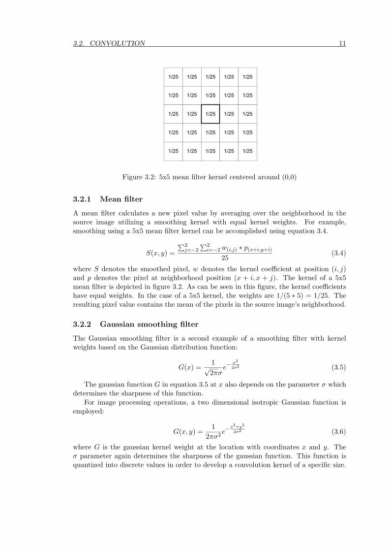
3.2.1 Mean filter
A mean filter calculates a new pixel value by averaging over the neighborhood in thesource image utilizing a smoothing kernel with equal kernel weights. For example,smoothing using a 5x5 mean filter kernel can be accomplished using equation 3.4.
S(x, y) =∑2
j=−2
∑2i=−2 w(i,j) ∗ p(x+i,y+i)
25(3.4)
where S denotes the smoothed pixel, w denotes the kernel coefficient at position (i, j)and p denotes the pixel at neighborhood position (x + i, x + j). The kernel of a 5x5mean filter is depicted in figure 3.2. As can be seen in this figure, the kernel coefficientshave equal weights. In the case of a 5x5 kernel, the weights are 1/(5 ∗ 5) = 1/25. Theresulting pixel value contains the mean of the pixels in the source image’s neighborhood.
3.2.2 Gaussian smoothing filter
The Gaussian smoothing filter is a second example of a smoothing filter with kernelweights based on the Gaussian distribution function:
G(x) =1√2πσ
e−x2
2σ2 (3.5)
The gaussian function G in equation 3.5 at x also depends on the parameter σ whichdetermines the sharpness of this function.
For image processing operations, a two dimensional isotropic Gaussian function isemployed:
G(x, y) =1
2πσ2e−
x2+y2
2σ2 (3.6)
where G is the gaussian kernel weight at the location with coordinates x and y. Theσ parameter again determines the sharpness of the gaussian function. This function isquantized into discrete values in order to develop a convolution kernel of a specific size.

12 CHAPTER 3. IMAGE PROCESSING OPERATIONS
0,002969 0,013306 0,021938 0,013306 0,002969
0,013306 0,059634 0,09832 0,059634 0,013306
0,013306 0,059634 0,09832 0,059634 0,013306
0,002969 0,013306 0,021938 0,013306 0,002969
0,021938 0,09832 0,1621 0,09832 0,021938
Figure 3.3: 5x5 gaussian filter kernel with σ = 2 centered around (0,0)
Figure 3.4: application of mean filter (middle) and gaussian filter (right)
For example, a 5x5 Gaussian kernel with σ = 2 can be represented as depicted in figure3.3. The kernel weights shown in the figure have been calculated using equation 3.6.
Application of both mean filter and gaussian filter to an example image yields theresult as shown in figure 3.4. The left image shows the original image, the middle imageshows the application of the mean filter and the right image shows the application ofthe gaussian filter. The right image shows a little more detail compared to the middleimage but requires more complex calculations.
3.2.3 Algorithmic representation of the convolution operation
Listing 3.1 provides the algorithmic representation of the convolution operation. Usingthis algorithm, the source image s is scanned on a row first basis. The output pixel valuein d is calculated by multiplying the corresponding neighborhood pixels in s with thekernel weights in w. An odd-sized square kernel centered around (0, 0) is assumed, henceit is indexed (both horizontally and vertically) from −(w.width− 1)/2 to +(w.width−1)/2).
3.3. COLOR SPACE CONVERSION 13
Listing 3.1: Pseudo code for convolution operation
%% s = source image%% d = de s t i n a t i on image%% w = kerne l window
for ( i , j ) := 1 to ( s . he ight , s . width ) dobegin
for (m, n) := (−(w. height −1)/2 , −(w. width−1)/2) to+(w. height −1)/2 , +(w. width−1)/2) do
begind [ i , j ] = s [ i+m, j+n ] ∗ w[m, n ] ;
end ;end ;
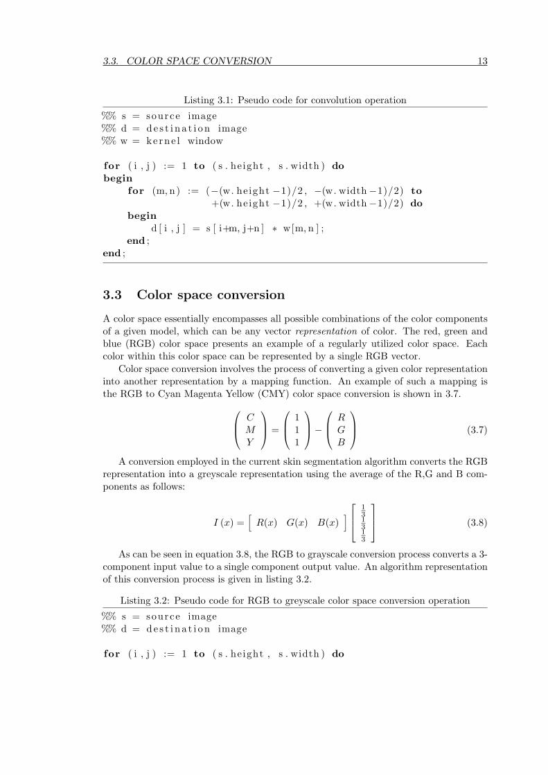
3.3 Color space conversion
A color space essentially encompasses all possible combinations of the color componentsof a given model, which can be any vector representation of color. The red, green andblue (RGB) color space presents an example of a regularly utilized color space. Eachcolor within this color space can be represented by a single RGB vector.
Color space conversion involves the process of converting a given color representationinto another representation by a mapping function. An example of such a mapping isthe RGB to Cyan Magenta Yellow (CMY) color space conversion is shown in 3.7. C
MY
=
111
−
RGB
(3.7)
A conversion employed in the current skin segmentation algorithm converts the RGBrepresentation into a greyscale representation using the average of the R,G and B com-ponents as follows:
I (x) =[
R(x) G(x) B(x)] 1
31313
(3.8)
As can be seen in equation 3.8, the RGB to grayscale conversion process converts a 3-component input value to a single component output value. An algorithm representationof this conversion process is given in listing 3.2.
Listing 3.2: Pseudo code for RGB to greyscale color space conversion operation
%% s = source image%% d = de s t i n a t i on image
for ( i , j ) := 1 to ( s . he ight , s . width ) do

14 CHAPTER 3. IMAGE PROCESSING OPERATIONS
begind( i , j ) := (1/3) ∗ s ( i , j ) .R + (1/3) ∗ s ( i , j ) .G + (1/3) ∗ s ( i , j ) .B
end ;
3.4 Erosion and dilation
Erosion and dilation are two examples of morphological operations. Applying these op-erations changes the structure or form of an image, the element used to transform animage is called a structuring element. Both greyscale and binary morphological opera-tions exist. However, only the binary versions are of interest to this project since theseversions are used in the skin segmentation algorithm2.
The set resulting from the dilation of an input image A with a structuring elementB can be denoted as follows:
A⊕B = {z|[(B̂
)z∩A] ⊆ A} (3.9)
The dilation of A by B is the set of all displacements z of B denoted B̂, such thatB̂ and A intersect by at least one element. Algorithmically, the process of performing adilation with a square shaped structuring element can be described as follows:
Listing 3.3: Pseudo code for a binary dilation operation
%% A = source image%% B = s t ru c tu r i n g element%% C = r e s u l t i n g image
for ( i , j ) := 1 to (A. height , A. width ) do beginsum := 0 ;for (m, n) := (−(B. height −1)/2 , −(B. width−1)/2) to
+(B. height −1)/2 , +(B. width−1)/2) dobegin
sum := sum + A[ i+m, j+n ] ;end ;
i f (sum > 0) thenC[ i , j ] := 1 ;
elseC[ i , j ] := 0 ;
end i f ;end ;
The binary erosion of an input image A with a structuring element B can be denotedas follows:
2The erosion and dilation operations used in the skin segmentation algorithm operate on the outputof threshold operations. Therefore, only binary erosion and dilation are of interest to this project.

3.5. LOCAL COUNT AND ABSOLUTE DIFFERENCE 15
AB = {z| (B)z ⊆ A} (3.10)
Thus, the erosion of A by B is the set of all displacements z of B such that B andA overlap by all elements. The algorithmic representation of an erosion is similar to thedilation with the exception that the if-condition should read:
Listing 3.4: Pseudo code excerpt for a binary erosion operation. . .
i f (sum = B. s i z e ) thenC[ i , j ] := 1 ;
elseC[ i , j ] := 0 ;
end i f ;. . .
The binary opening of an image can be achieved by first applying an erosion followedby a dilation. This operation effectively smoothes the the contour of objects in the image.When applying a dilation followed by an erosion, the result consists of the binary closingof that image. This operation also smoothes the contours of objects but fuses narrowbreaks in the contours.
Figure 3.5 shows the result of an input image (a) processed with a dilation (b), erosion(c), opening (d) and closing (e). For a detailed discussion on mathematical morphology,please refer to [11].
3.5 Local count and absolute difference
The binary local count filter scans a kernel across the binary input image and counts theamount of pixels with a value of 1 within the neighborhood. To a certain extend, theeffect of this operation is similar to that of a uniform filter with kernel weights of 1. Theuniform filter however calculates the average of the pixels in the neighborhood, whereasthe local count calculates the sum of these pixels.
To provide a basic method of motion estimation, the skin segmentation also employsthe computation of the absolute difference between two grey scale images based on 3.11.
D(x) = |It(x)− It−1(x)| (3.11)
where D(x) denotes the absolute difference at location x, It(x) and It−1(x) denote theintensity of a pixel at location x in a frame at time t and t− 1 respectively.
It provides information on the intensity change between two subsequent grey scaleimages. As opposed to the local count operation, this is a point operation and thus itdoes not require the neighborhood of each pixel to calculate the output pixel.
3.6 Summary
The image processing operations discussed in this chapter are used in the targeted skinsegmentation algorithm. These operations can be classified either as point operations or

16 CHAPTER 3. IMAGE PROCESSING OPERATIONS
a b
c d
e
Figure 3.5: application of a dilation (b), erosion (c), opening (d) and closing (e) operation
local operations. Thus the computation of the results require either only the input pixelor its neighborhood (defined by the kernel of the operation). It is worth noting that thelocal operations share a similar window scanning method.

Implementation considerations 4The mapping of image processing operations such as those mentioned in the previouschapter onto a suitable platform requires knowledge of the related implementation as-pects. This chapter introduces the aspects and concepts related to parallel processingsystems, flexibility and possible candidate implementation platforms. A choice for themost suitable platform is presented at the end of this chapter.
4.1 Exploiting Parallelism
Through the exploitation of inherent parallelism, operations can be executed consider-ably faster compared to sequential implementations. Many image processing operationsare suited for implementation utilizing a certain type of parallelism because of the lackof data dependencies. Before discussing appropriate implementation platforms, a briefoverview of relevant parallelism concepts is presented. First, instruction level parallelismis introduced. This is a type of parallelism supported by modern processors and thus isbeing used in the current software implementation of the skin segmentation algorithm.Second, task level parallelism is introduced. This is a type of parallelism as perceivedfrom an application perspective. The discussion is by no means intended to be a com-prehensive and complete overview. For a detailed discussion, the reader is referred toliterature on parallel processing such as [8] and [12].
4.1.1 Instruction level parallelism
Probably the most popular taxonomy on instruction level parallelism was proposed byFlynn [9] in 1966. It introduces the following categorization based on instruction anddata streams:
• single instruction stream, single data stream (SISD): this category is also denotedas ’uniprocessors’ and utilize a single instruction which operates on a single dataset;
• single instruction stream, multiple data stream (SIMD): a single instruction oper-ates on multiple data sets, multimedia extensions of modern processors are oftenSIMD style instruction;
• multiple instruction, single data (MISD): multiple instructions operate on a singledata set, this is a quite uncommon category;
• multiple instruction, multiple data (MIMD): multiple instructions operate on mul-tiple data sets, this category comprises multiprocessor systems which utilize mul-tiple processors.
17
18 CHAPTER 4. IMPLEMENTATION CONSIDERATIONS
The general purpose uniprocessor presents an example of the commonly utilizedSISD category. The traditional operation of such processors consists of the fetch-decode-execute-write back or a somehow similar execution cycle. First, an instruction is fetchedfrom memory, then it is decoded and the relevant functional unit1 is addressed, the ex-ecution takes place in the functional unit and after completion the results are writtenback into memory. This execution cycle allows for a technique denoted pipelining. Thistechnique allows the staged and concurrent operation inside the execution cycle. Forexample, at a certain moment instruction A can be decoded while simultaneously in-struction B is being fetched from memory. Pipelining is a common technique utilized inmany processors presently available.
It is possible to further parallelize execution through the provision of multiple parallelexecution pipelines. This technique, denoted as super scalar execution, allows for aninstruction to be dispatched to an available pipeline. Effectively, multiple instructionscan be present in the different pipelines concurrently.
Although these techniques allow the execution of multiple instructions per clock cycle,the data dependencies between subsequent instructions and the non-linear executionflow introduced through conditional branches2 pose a limit on the effectiveness of thesetechniques. Since a conditional branch can depend on the result of an instruction whichis executed at the moment the branch is evaluated, the processor is unable to decidewhich consequent instruction to fetch.
Several initiatives to alleviate this problem exist, either depending on hardware oron software support. A technique commonly found in modern digital signal processorsis based on an instruction format which encodes independent operations into a singleinstruction. This instruction format is denoted Very Long Instruction Word (VLIW).During execution, the operations present in the instruction are separately dispatchedto different execution pipelines. It is vital that these operations do not share datadependencies, it is the task of the compiler to select operations which can be executedindependently.
The concepts of parallelism present in modern processors have been discussed in theliterature. For a detailed discussion of architectural aspects of parallelism, the reader isreferred to [15].
4.1.2 Task level parallelism
Another level of parallelism can be found at the task level of an operation. By examin-ing the operation to be performed, different tasks may be identified which can operateindependently without introducing any data hazards.
Since this level of parallelism depends entirely on the type of operation, it is difficultto provide a general framework for the categorization of task level parallelism.
Task level parallelism can be implemented as thread level parallelism, where each taskis assigned to an execution thread. This thread can then be executed on an availableprocessing unit. An important aspect introduced by utilizing thread level parallelism is
1Examples of functional units are the Arithmetic and Logic Unit (ALU) and Floating Point Unit2A conditional branch determines if the current execution flow can continue by evaluating a certain
register or flag

4.2. FLEXIBILITY 19
the communication overhead involved. Different threads may need to communicate withan arbiter or other threads in order to successfully finish their respective operations.
Algorithmic representation often need to exhibit explicit constructs (for example thebalanced tree construct) and communication operations to utilize task level parallelism.A detailed discussion of parallelism concepts and the design of parallel algorithms canbe found in [12].
4.2 Flexibility
The term ”flexibility” is a rather broad and subjective term. Generally, the designproblem is often confronted with the compromise between flexibility and performanceimprovement. Flexible systems most likely offer less performance compared to less flex-ible but fully optimized systems. It is therefore necessary to examine the problem moreclosely to provide some concrete criteria for the system to be developed. In the contextof this project we therefore define the following relevant concepts:
• flexibility of function; from a functional perspective the system should performthe image processing operations as defined by the ”skin segmentation” algorithmemployed (as described in detail in appendix A). However, this algorithm will beimproved and therefore modified within the near future. It is therefore requiredthat a next version of this algorithm can be executed by the system with as littleeffort as possible;
• flexibility of operation; several parts of the algorithm contain parameters whichinfluence the operation they perform. These parameters should not be fixed inthe system but a possibility should be provided to modify these parameters duringsystem operation;
• flexibility of use; from the end-user perspective the system needs to be flexible in(daily) use. Therefore, an easy to operate or connect system is preferred over asystem which requires complex installation. Judging by the context of this projecthowever, this concept is of less importance although it should be considered iffeasible.
4.3 Implementation platforms
A variety of different implementation platforms exist, each exhibiting specific character-istics which may or may not aid in the acceleration of image processing operations. Thefollowing sections provide a short overview of the possible implementation platforms andtheir effectiveness on the implementation of real-time image processing operations.
4.3.1 General purpose processor
General purpose processors (GPP’s) provide an execution environment for general pur-pose processing tasks. The instruction set architecture is suited to different types ofcomputations. Some architectures are extended with instructions for specific processing

20 CHAPTER 4. IMPLEMENTATION CONSIDERATIONS
tasks. The Pentium processor is an example of a general purpose processor with SIMDtype extensions for multimedia processing. It exhibits instruction level parallelism tech-niques such as those mentioned in section 4.1.1.
General purpose processors provide little support for true task parallelism, althoughemulated parallelism can be achieved by utilizing several threads in an application. How-ever, threads will not be executed truly in parallel since the instructions will be executedsequentially.
High level software development for general purpose processors requires little knowl-edge of the processor architecture. It is therefore suitable for flexible implementationsof image processing operations.
4.3.2 Digital signal processor
Digital signal processors (DSPs) are especially suited for specific signal processing al-gorithms. Both processor and instruction set architecture utilize special constructs tooptimize execution times for these algorithms. Furthermore, DSPs might use SIMD styleinstructions to implement parallel processing.
Software development for digital signal processors often requires knowledge of theprocessor architecture to develop an efficient implementation. It is therefore less suit-able for flexible implementation of image processing operations compared to the generalpurpose processor.
The Philips Nexperia processor (also known as the Trimedia) is an example of a digitalsignal processor specifically designed for MPEG encoding and decoding. Its instructionset is based on the VLIW concept and thus it provides means for parallel execution ofinstructions.
The graphics processing unit (GPU) commonly found on PC add-on boards, is an-other example of a digital signal processor. These units most often find their implemen-tation as accelerator for specialized 3D graphics processing operations.
4.3.3 Application specific IC
Processors as mentioned in the previous sections employ a fixed hardware architecturewhich is programmable in the sense that it is able to execute user algorithm instructions.In contrast, application specific integrated circuits (ASICs) contain optimized circuitimplementations of the desired functionality in hardware.
Hardware description languages (HDLs) can be used to develop an ASIC. Theselanguages are syntactically similar to imperative languages but provide means to describeparallel hardware circuits rather than a sequence of processor instructions. Consequently,a compiler for a hardware description language produces a hardware circuit descriptioninstead of low-level processor instructions.
Another fundamental difference is that hardware circuits inherently operate concur-rently and thus provide the possibility to develop parallel structures. Moreover, becauseof this parallel nature, development of sequential operations requires special techniquessuch as finite state machines.

4.4. CONCLUSION 21
4.3.4 Programmable hardware
Several different types of programmable hardware exist, but the predominant type cur-rently is the Field Programmable Gate Array (FPGA). The term ”field programmable”can be attributed to the fact that once the FPGA is fabricated, its operation can beadapted ”in the field”. This is contrary to the ASIC which cannot be adapted oncefabricated.
An FPGA contains a large amount of programmable logic cells, each cell typicallycontaining several registers and logic and performs a variety of different functions ac-cording to its configuration. The cells are interconnected and thus provide the possibilityto develop logic circuits of a larger scale.
Whereas an ASIC consists of fixed but highly optimized circuitry, FPGA’s providea flexible configuration through the utilization of the programmable logic cells and in-terconnections. Consequently, ASIC implementations often achieve higher performancecompared to FPGA implementations.
Specification and validation of functionality may follow the same approach as forASIC development, the actual implementation however differs in the fact that an ASIChas to be manufactured while an FPGA design may be adapted at any time.
4.4 Conclusion
From the implementation platforms presented, each has advantages and limitations withrespect to efficient implementation of image processing operations. General purposeprocessors provide a considerable degree of flexibility but often do not allow a paral-lel implementation of image processing operations. Digital signal processors provide amore efficient and thus better performing implementation compared to general purposeprocessors, but still do not allow true parallel execution of the image processing opera-tions. An ASIC implementation would provide the most efficient and best performingimplementation but lacks the required flexibility to adapt the design when necessary.Furthermore, the cost and time associated with the manufacturing of an ASIC presentan important reason not to consider it as an interesting implementation platform for ourproject.
Consequently, the FPGA platform yields the best balance between flexibility andperformance. The design can be adapted relatively easily by modifying the source filesand re-synthesizing the design. A parallel implementation is possible by developingconcurrent hardware circuits (blocks) for each image processing operation.
Development boardTo design and implement the accelerator on an FPGA, a suitable development board
is required. This board should provide a communication interface capable of transferringthe images to and from the FPGA.
After a careful investigation, we chose to utilize the Digilent XUP V2P board [14]for our accelerator. It is a low-cost FPGA board containing a Virtex II Pro FPGAand various communication interfaces. The manufacturer provides a fully functionalcommunication stack for 10/100 Mbps ethernet interface, effectively reducing the effortrequired to obtain an operational communication link.

22 CHAPTER 4. IMPLEMENTATION CONSIDERATIONS
For the remainder of this thesis we will refer to the programmable hardware imple-mentation using an FPGA simply as ”hardware implementation”.
Architecture design 5This chapter describes the architectural design of the developed system. It also states theimplementation constraints derived from the system real-time requirements.
5.1 Architecture
The architecture of the system describes the components involved, their function andtheir respective interfaces. The next paragraphs present a description of the overallsystem architecture and the accelerator architecture. First, the flexibility criteria im-posed on the architecture are discussed, then the architectures of the overall system, theaccelerator and pixel processing pipeline are presented.
5.1.1 Criteria for architecture design
In the previous chapter we defined the three flexibility criteria for the accelerator to bedeveloped. From these general criteria we can derive requirements for the system andaccelerator architecture.
The flexibility of use criterion depends both on the accelerator and on the driversoftware on the host PC. The accelerator should provide sufficient means to aid in theflexible use by the user. Connecting and disconnecting should therefore be straightforward and should not require much user interaction.
To provide flexibility of function, it should be possible to adapt the architecture ofthe algorithm in hardware. There are several different methods to implement such afunctionality:
1. A very flexible method can be found by implementing an architecture similar tothose utilized by (digital signal) processors. This will provide the highest flexibilitybut the least performance improvement;
2. Using a micro programmable architecture, operations can be implemented by de-scribing each operation as a sequence of micro operations. The implementationwould involve implementing the micro operations and programming the algorithmby specifying the required micro operations. This will provide a lower degree offlexibility but a higher improvement in performance compared to the general pur-pose architecture approach.
3. A fixed implementation where each algorithm operation is implemented directlyin the reconfigurable hardware. This will provide the highest performance but theleast flexibility.
23

24 CHAPTER 5. ARCHITECTURE DESIGN
We decided to implement the operations in hardware (option 3 above) since thisprovides the highest performance improvement. Furthermore, since we utilize an FPGA,we can implement different algorithms by redesigning only the required parts. Thismethod is therefore not completely inflexible and still allows algorithm modifications.
Flexibility of operation presents an important criterion for the architecture. It isdesirable to control the parameters of several predefined algorithm operations when theaccelerator is in use. The architecture should therefore provide the possibility to accessand modify such parameters.
5.1.2 System architecture
The overall system architecture is depicted in figure 1.1. The system consists of a hostPC connected to the accelerator through an Ethernet network connection. The PCcaptures images from a webcam at a frame rate of 25 frames per second and transfersthese images to the accelerator. The accelerator processes the images and returns theresults back. This architecture allows flexibility of use since it can be connected usinga regular network cable. The FPGA allows flexibility of function since the hardwaredescription of the algorithm can be adapted. Flexibility of operation will be achieved byallowing algorithm parameters to be changed at run-time.
Considering the Ethernet network connection used and the fact that very high band-width utilization is essential for the overall system performance, we adopted UDP forour network communication protocol. There are two packet types: data (also referredto as pixel packets) that carry consecutive pixel- or accelerator output information andconfiguration packets used for system configuration at run-time.
The pixel packets are 1358 bytes long and contain 320 pixels using 4 bytes per pixel(320*4 = 1280 pixel bytes). The remaining 78 bytes are used for the following headers:accelerator (38), UDP (8), IP (18) and MAC (14 bytes). The accelerator header containsa frame number indicating which frame the pixels in this packet belong to and an x andy coordinate indicating the spatial location of the first pixel present in the packet. Tosupport a multiple camera setup1, a camera identification number indicates the sourceof the pixels. The accelerator output consists of 4 bytes per pixel which contain theabsolute difference, grey value and skin segmented output.
The configuration packets contain parameters values for the accelerator. These pa-rameters determine the operation of several image processing operations present in theaccelerator. The configuration packets have the same size as the pixel packets in or-der to simplify the protocol handling on the PowerPC processor present in the FPGA.The meaningful part of the payload is only 80 bytes. This is, however, not a big issueconsidering that configuration packets are usually not intermingled with pixel data atrun-time. Please refer to appendix B for a complete overview of the pixel packet andconfiguration packet structure.
1A multiple camera setup allows several cameras to be connected to the host PC and might be usedfor example to improve the accuracy of hand gesture recognition. The accelerator supports such a setupby providing a camera identification number in the accelerator header of the pixel packets.

5.1. ARCHITECTURE 25
5.1.3 Accelerator architecture
The architecture of the accelerator is depicted in figure 5.1 and consists of several distinctcomponents2 interconnected by busses. The following components are present:
• Ethernet media access layer component (EMAC): the EMAC is responsible forreceiving and sending of data packets. When an incoming packet is received, aprocessor interrupt will be raised in order to transfer the packet to the data mem-ory;
• Processor: the processor is responsible for the overall coordination of the com-ponents present. Furthermore, it must ensure a timely transfer of data betweenthe components. The processor transfers incoming and outgoing packets from andto the EMAC, and it transfers packets to and from the pixel processing pipeline(PPP) subsystem;
• Data memory: this memory is used as an intermediate buffer between the ethernetcomponent, the processor and the pixel processing pipeline subsystem;
• Instruction memory: this memory contains the program code (instructions) for thePowerPC processor;
• Interrupt controller; the processor contains a single interrupt port but the archi-tecture contains two interrupt sources: the EMAC and the PPP. The interruptcontroller is required to multiplex the two interrupt signals into a single signal;
• Pixel processing pipeline subsystem: the PPP is responsible for the image process-ing operations performed on the pixel data;
• PLB and OPB bus; the Processor Local Bus (PLB) and On-Chip Peripheral Bus(OPB) provide shared communication paths between the different components;
• Bus bridge; the system comprises two bus types: a high-speed (PLB) bus and alow-speed (OPB) bus. The bridge connects these two busses and takes care of thetiming;
• PPP Bus Interface (IPIF): provides an interface to the PLB bus in order to simplifythe design of the PPP subsystem. It also provides two additional FIFO’s fortemporal storage.
• Universal Asynchronous Receiver Transmitter (UART); the UART provides theprocessor with a standard input and standard output for status and debug infor-mation to an external computing system.
The interaction of the different components directly involved in processing pixel pack-ets will be illustrated by a simple example of a single receive packet event. The exampledemonstrates the pixel packet dataflow in the accelerator and is shown in figure 5.2.
The following sequence of actions will be executed upon receiving a pixel packet:2The EMAC, PLB, OPB, Bus Bridge, IPIF, UART and Interrupt controller are standard components
provided by Xilinx.

26 CHAPTER 5. ARCHITECTURE DESIGN
PowerPC
405
processor
Processor Local Bus (PLB) 64 bit
On-Chip Peripheral Bus (OPB)
UART
Ethernet MAC
Data Memory
Bus Interface
(IPIF)
BUS2IP
FIFO
IP2BUS
FIFO
Pixel Processing Pipeline
(PPP) Subsystem
RS232
status and debug
information
10/100 Ethernet
transfer of pixel
packets
Virtex 2 Pro FPGA
Instruction Memory
Interrupt controller
PLB2OPB Bridge
Figure 5.1: system architecture
1. an incoming pixel packet arrives at the EMAC;
2. the EMAC receives the packet in its internal buffer and generates a processorinterrupt;
3. the processor starts the interrupt handler which transfers the packet into the datamemory and analyzes the packet header;
4. the processor transfers the packet to the pixel processing pipeline input buffer(BUS2IP);
5. the PPP processes the packet on a pixel by pixel basis and stores the results in thePPP output buffer (IP2BUS), and generates an interrupt when a complete pixelpacket has been processed;
6. the processor executes the interrupt handler which transfers the packet back intoits data memory;

5.1. ARCHITECTURE 27
EMAC receives packet
Processor handles
interrupt: copy packet to
data memory
Incoming ethernet packet
EMAC generates processor interrupt
Processor copy packet to
PPP IPIF
PPP processes packet
Processor handles
interrupt: copy packet to
data memory
Processor transfers packet
to EMAC
EMAC sends packet
PPP generates processor interrupt
Figure 5.2: example pixel packet flow
7. the processor transfers the packet to the EMAC and orders the EMAC to transmitthe packet to the host PC;
8. the EMAC transmits the packet to the host PC using the direct Ethernet connec-tion.
Instead of transferring incoming packets directly to the PPP, the packets are firsttransferred to the processor data memory. The reason is that the processor should beable to examine the packet headers in order to determine whether the packet should betransferred to the PPP or not. Configuration packets for example must not be transferredto the PPP but interpreted by the processor instead. In addition, there may be networktraffic unrelated to the accelerator which need to be discarded.
To resolve temporary and irregular delays in the accelerator, for example caused bytwo interrupts to be serviced simultaneously, two IPIF FIFO buffers which can containmultiple packets are used.
5.1.4 Pixel Processing Pipeline subsystem architecture
The skin segmentation algorithm as presented in appendix A can be divided 10 dependentstages. Each stage contains a certain amount of different independent operations whichcan be performed simultaneously.
The PPP subsystem implements the building blocks of this algorithm. We decidedto implement the PPP by utilizing a pixel pipelined architecture in order to be able to

28 CHAPTER 5. ARCHITECTURE DESIGN
process several pixels simultaneously. The amount of pixels which can be processed at asingle moment depends on the amount of stages present in the pipeline.
Figure 5.3 shows the architecture of the pixel processing pipeline. The operationsindicated correspond to the operations of the skin segmentation algorithm. The dottedlines between the pipeline stages represent pipeline registers which contain the temporaryresults from the preceding stage. The pipeline controller is responsible for the coordina-tion of the entire processing pipeline. It determines when all pipeline stages have finishedprocessing in order to start the next pipeline cycle.
The image buffer present in the algorithm is used to determine the absolute differencebetween two consecutive images. It was decided not to implement this buffer in hardware.This would either require a large amount of block RAM or add additional complexityfor interfacing external Dual Data Rate RAM. Instead, the host PC is responsible forproviding the required pixel values. This can be accomplished if the host PC driverutilizes at least two image buffers. It includes the corresponding pixels of the previousimage when transmitting an image to the accelerator.
5.2 Implementation constraints
The accelerator is required to process video frames at 25 frames per second. Eachindividual video frame has a width of 640 pixels and a height of 480 pixels. Each pixelconsists of a red, green and blue color components, each represented using a single byte.Additionally, each pixel contains an 8 bit grey value of the corresponding pixel from theprevious frame. Thus each pixel is represented by 32 bits.
5.2.1 Network bandwidth
The decision was made to transfer the video frames to and from the accelerator withoutdata compression. The advantage of uncompressed data is that we do not require botha compression component on the host PC and a decompression component within theaccelerator. However, this approach requires a higher amount of bandwidth comparedto the case when data compression is used.
It is also important to consider the communication overhead introduced when uti-lizing the packet based networking communication. The TCP/IP communication stan-dard [26] states that a maximum of 1500 data bytes can be transferred per packet.Additional control and error detection information is appended to the data to allowcommunication control between the host PC and the accelerator.
At any given video resolutions and frame rate, the following bandwidth requirementapproximation holds:
BW = depthbits per pixel ∗ Iwidth ∗ Iheight ∗Rframe ∗ Foverhead (5.1)
where the depth indicates the amount of bits required to represent a pixel, Iwidth andIheight indicate the image dimensions, R indicates the frame rate and F represents theoverhead factor caused by the additional header data present in a pixel packet.

5.2. IMPLEMENTATION CONSTRAINTS 29
10
1
2
3
4
5
76
9
8
11
color
space
convert
color
space
convert
color
space
convert
dis-
similarity
division
squaring
thres-
holding
thres-
holding
local
count
thres-
holding
thres-
holding
closing
uniform
filter
absolute
difference
AND
dilation
1 2 3
4 5 14
9
10
12 13
16
18
Input pixel
[R,G,B, Grey T-1]
Pipeline Controller
6
Output
[Abs Diff, Grey T, Skin Segmentation]
mean
subtract
mean
subtract
squaring squaring
7 8
absolute
differ-
ence
15
17
19
20
Figure 5.3: pixel processing pipeline architecture
As previously explained, the pixel packets contain 1280 bytes pixel data and 78additional bytes required for protocol headers (as mentioned in section 5.1.2), resultingin communication overhead factor of approximately 6%.
Given a pixel depth of 32 bits, a frame rate of 25 frames per second and a networkpacket overhead factor of 6%, the resulting bandwidth requirements are 62,11 Mbpsfor image dimensions of 320x240, 248,44 Mbps for 640x480 and 636 Mbps for 1024x768pixels. Since our implementation utilizes a 10/100 Mbps Ethernet MAC, it is limitedto image dimensions of 320x240 pixels, however a gigabit Ethernet MAC would enable

30 CHAPTER 5. ARCHITECTURE DESIGN
image dimensions of either 640x480 or 1024x768.
5.2.2 Accelerator throughput
We decided to utilize communication packets containing 320 pixels per packet. Theamount of packets to be processed by the accelerator can thus be estimated as follows:
Rpacket =Iwidth ∗ Iheight
320∗Rframe (5.2)
where Iwidth and Iheight denote the image dimensions and Rframe indicates the framerate. With image dimensions of 640x480 pixels and a frame rate of 25 frames per second,the processing rate Rpacket is 24000 packets per second. Since Ethernet communicationallows full duplex operation3 this effective packet processing rate doubles to 48000 packetsper second.
To test the PowerPC software overhead of packet handling, we developed two packethandling approaches. The first approach was based on utilization of a micro kernel4 withsupport for processes. We developed processes for receiving packets from the EMACand the PPP. The second approach involved two interrupt handlers for the same tasks.Through empirical observation we concluded that the process based approach was limitedin performance due to the context switching overhead involved. We therefore decided toimplement the interrupt based approach.
The interrupt routines are required to finish processing within the time available fora single packet. Assuming the CPU clock frequency is 300 MHz, the following amountof clock cycles are available to each routine:
Tmax =Fclock
Rpacket=
300 ∗ 106
48000= 6250 clock cycles (5.3)
where Rpacket indicates the full duplex packet processing rate and Fclock indicates theclock frequency. The PowerPC reference manual [30] states that the typical amount ofclock cycles required per instruction is 1. Thus, each routine may consist at maximumof approximately 6250 instructions.
Since the accelerator utilizes a communication bus, it is important to consider theavailable bus bandwidth. The bus conforms to the Processor Local Bus standard [6]and provides a data transfer width of 64 bits. The PLB bus operates at a maximumfrequency of 100 MHz. When utilizing burst transfers 5 the accelerator is effectively ableto transfer 64 bits of data per bus clock cycle. Thus, the available bus bandwidth canbe approximated as follows:
3Full duplex operations allows for simultaneous sending and receiving of data. On the contrary, halfduplex only allows for either sending or receiving of data at a given moment.
4A micro kernel is a minimal implementation of an operating system. It supports minimal operatingsystem functionality such as thread management and inter-process communication. The micro kernelprovided with the FPGA and which was used for our evaluation is called Xilkernel.
5Burst transfers consist of a sequence of data transfers initiated by a single command. The effectivethroughput of burst transfers can be as high as one data transfer per clock cycle. On the contrary, singledata transfer require a command for each transfer requested.
5.3. CONCLUSION 31
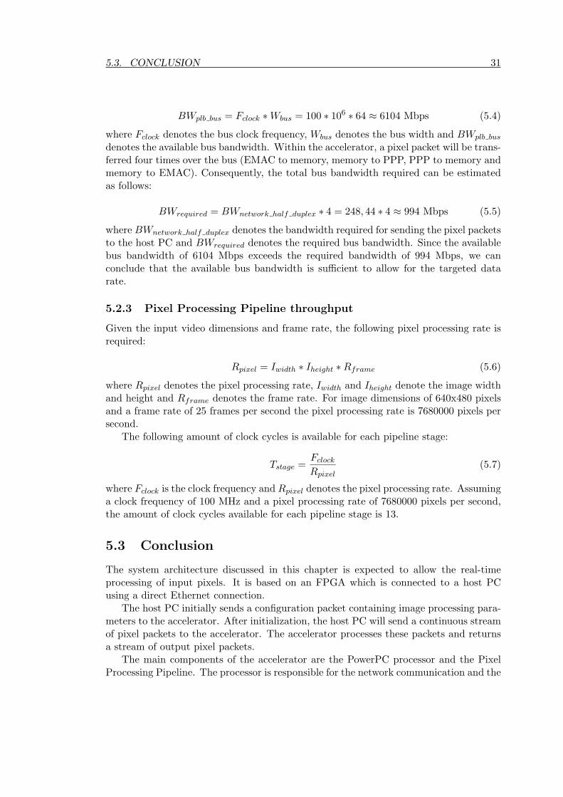
BWplb bus = Fclock ∗Wbus = 100 ∗ 106 ∗ 64 ≈ 6104 Mbps (5.4)
where Fclock denotes the bus clock frequency, Wbus denotes the bus width and BWplb bus
denotes the available bus bandwidth. Within the accelerator, a pixel packet will be trans-ferred four times over the bus (EMAC to memory, memory to PPP, PPP to memory andmemory to EMAC). Consequently, the total bus bandwidth required can be estimatedas follows:
BWrequired = BWnetwork half duplex ∗ 4 = 248, 44 ∗ 4 ≈ 994 Mbps (5.5)
where BWnetwork half duplex denotes the bandwidth required for sending the pixel packetsto the host PC and BWrequired denotes the required bus bandwidth. Since the availablebus bandwidth of 6104 Mbps exceeds the required bandwidth of 994 Mbps, we canconclude that the available bus bandwidth is sufficient to allow for the targeted datarate.
5.2.3 Pixel Processing Pipeline throughput
Given the input video dimensions and frame rate, the following pixel processing rate isrequired:
Rpixel = Iwidth ∗ Iheight ∗Rframe (5.6)
where Rpixel denotes the pixel processing rate, Iwidth and Iheight denote the image widthand height and Rframe denotes the frame rate. For image dimensions of 640x480 pixelsand a frame rate of 25 frames per second the pixel processing rate is 7680000 pixels persecond.
The following amount of clock cycles is available for each pipeline stage:
Tstage =Fclock
Rpixel(5.7)
where Fclock is the clock frequency and Rpixel denotes the pixel processing rate. Assuminga clock frequency of 100 MHz and a pixel processing rate of 7680000 pixels per second,the amount of clock cycles available for each pipeline stage is 13.
5.3 Conclusion
The system architecture discussed in this chapter is expected to allow the real-timeprocessing of input pixels. It is based on an FPGA which is connected to a host PCusing a direct Ethernet connection.
The host PC initially sends a configuration packet containing image processing para-meters to the accelerator. After initialization, the host PC will send a continuous streamof pixel packets to the accelerator. The accelerator processes these packets and returnsa stream of output pixel packets.
The main components of the accelerator are the PowerPC processor and the PixelProcessing Pipeline. The processor is responsible for the network communication and the

32 CHAPTER 5. ARCHITECTURE DESIGN
overall system control, the pixel processing pipeline is responsible for the implementationof the skin segmentation algorithm. The implementation of the pixel processing pipelineremains fixed during run-time. However, it can be modified by adapting the source codeof the algorithm and resynthesis of the design. The parameters of the skin segmen-tation algorithm can be updated when the system is operational by sending dedicatedconfiguration packets to the accelerator.
Since the selected development board contains a 100 Mbps Ethernet network con-nection, an image resolution of 320x240 pixels can be supported at a frame rate of 25frames per second. A gigabit Ethernet connection would allow image resolutions of640x480 pixels at the same frame rate.

Implementation 6The main components of the architecture of the accelerator are the PowerPC processorand the Pixel Processing Pipeline. Communication between host PC and the acceleratoroccurs via direct network connection. This chapter discusses the implementation of theaccelerator architecture and the pixel processing pipeline. The architecture provides ageneric framework for real-time image processing, whereas the pixel processing pipelineimplements the specific components for the skin segmentation algorithm. The first sectionprovides details on the implementation of the processor functionality, the second sectiondiscusses the pixel processing pipeline. Details on the timing and resource utilization ofthe PPP components are available in appendix D.
6.1 Processor functionality
The PowerPC processor is responsible for the overall coordination of the accelerator. Itimplements the functions required by the network protocol and controls the transfer ofpixel packets between the EMAC and the PPP. The following subsections provide detailson the network protocol and packet handling.
6.1.1 Network protocol selection
To establish a reliable communication link between the accelerator and the host PC,the processor should utilize the most suitable network protocol for the purpose. TheOpen System Interconnection (OSI) model for network communication [31] defines a setof layers that are involved in the communication between network connected systems.Generally, different software layers present within a system correspond to the differentOSI layers and implement the required functionality.
To minimize the network protocol overhead, we chose to use the User DatagramProtocol (UDP) [25] instead of the Transmission Control Protocol (TCP). The latterprotocol has significant control overhead in order to guarantee delivery and reception ofcorrect data packets. This might even result in packet retransmission when these havebeen damaged during transmission. The former protocol requires less overhead but doesnot guarantee delivery and reception of correct data packets. However, judging by thereal-time objective of our accelerator and the video application being used, we preferdamaged packets over packet retransmissions.
The performance issues encountered when developing high-speed communication ap-plications have been discussed in [5], [10] and [16]. The bottlenecks discussed in thesepapers are caused by the memory copy, checksum calculation and interrupt overheadintroduced by the network protocol handling. In [5] it is shown that several methodscan be used in order to increase the communication throughput. Several alternative
33

34 CHAPTER 6. IMPLEMENTATION
network protocols ( [21], [20]) have been proposed to reduce the processing overhead.However, these proposals have not yet been widely implemented and thus will result incompatibility problems if used in this project.
Our PowerPC software implementation uses the zero memory copy method, thiseffectively reduces the amount of packet transfers between software layers. Furthermore,our implementation omits the checksum calculation phase since this is allowed when usingthe UDP protocol. This prevents the host PC to detect errors in a packet but resultsin a significant communication performance improvement since checksum calculationsinvolves all data bytes in the packet.
6.1.2 Interrupt handling
The second task of the processor is coordination of the transfer of pixel packets betweenthe EMAC, data memory and the PPP. To minimize the transfer overhead, it was de-cided to implement this functionality using interrupt routines and direct memory access(DMA).
Currently two types of interrupts have been implemented: the EMAC receive packetinterrupt and the PPP packet processed interrupt. The former will be generated bythe EMAC whenever a network packet has been received, the latter when the PPP hasfinished processing a pixel packet.
The interrupt handling routine for the EMAC receive packet interrupt is responsiblefor transferring the packet from the EMAC component to the data memory. It also needsto identify the type of packet and process it accordingly. Currently the following typesof packets are recognized:
• Network protocol packets; both IP protocol and UDP protocol packets areprocessed. Furthermore, ICMP (”ping”) packets are recognized to provide thepossibility for testing the communication link between the accelerator and the hostPC. TCP and other network protocol packets will currently be discarded.
• ”Hello” packets; these packets will be send by the host PC in order to inform theaccelerator of the IP address and port number of the host PC. This information isrequired by the accelerator to return the processed pixel packets.
• Configuration packets; these packets contain parameter values for the PPP compo-nents. Upon receiving a configuration packet, the processor writes the appropriatevalues to the programmable registers of the PPP.
• Pixel packets; these packets contain pixels which will be transferred to the PPP inorder to be processed.
The interrupt handling routine for the PPP packet processed interrupt first transfersthe packets to the data memory. Then it appends the required protocol headers andfinally transfers the packets to the host PC.
To reduce the per-packet processing time, it was decided that the processor shouldnot be responsible for the administration of pixel packet header data. Consequently, theprocessor only transfers the packets to and from the PPP instead of also having to match

6.2. PIXEL PROCESSING PIPELINE 35
each processed pixel packet with the corresponding header. Thus, this responsibility isdelegated to the PPP by simply transferring the header data along with the pixel valuesinto the PPP.
As mentioned earlier, transfer of the pixel packets between the EMAC, system mem-ory and the PPP uses DMA. This method allows data transfer at a higher throughputcompared to programmed input/output1 (PIO) data transfer. A DMA operation trans-fers data from a specified source address to a destination address. Since the PLB bushas a width of 64 bits, a DMA operation effectively transfers 64 bits per clock cycle.It is required that both source and destination address are aligned on a 64 bit address,thus the processor needs to align the source and destination memory sections at such anaddress.
6.2 Pixel Processing Pipeline
This section discusses the implementation of our pixel processing pipeline. First, theimplementation of the pipeline architecture is presented. Next, the protocol used in thePPP is discussed. Then the color space conversion, erosion and dilation, uniform filterand local count components are discussed.
6.2.1 Pipeline implementation
The implementation diagram of the pixel processing pipeline is depicted in figure 6.1.In addition to the components mentioned in section 5.1.4, figure 6.1 shows the followingcomponents: input multiplexer, header bypass fifo, pipeline registers, delaying pipelineregisters and output demultiplexer.
The multiplexer and demultiplexer are required since a single PLB bus transfer con-tains 2 pixel values. The input multiplexer at the first pipeline stage therefore splits a 64bit value into two subsequent pixel values. The output demultiplexer in the last pipelinestage then concatenates two subsequent processed pixel values into a single 64 bit value.
Since the PPP is responsible for matching the processed pixel values to their corre-sponding header, a header bypass fifo is present. The fifo depth depends on the amountof pixel packets that can be present in the pipeline, and is determined by the amount ofpipeline stages and the initial latency of the local operations. These local operations re-quire several image lines to be present in their local buffers, and thus will contain severalpixel packets. A 5x5 local operation has an initial delay of approximately 2 image lines, a7x7 local operation approximately 3 image lines. Our implementation uses two pipelinestages with 5x5 local operations and one pipeline stage with a 7x7 local operation. Theheader fifo should therefore be able to accommodate at least 7 headers for 320x240 and14 for 640x480.
At the start of a new pixel packet, the input multiplexer transfers the header datato the header fifo. The output multiplexer then reads the header data from the headerfifo at the start of a new processed pixel packet. Both input multiplexer and outputdemultiplexer use a current pixel counter to identify the start of a new pixel packet.
1Programmed input/output denotes transfer of data involving processor instructions for each dataunit.

36 CHAPTER 6. IMPLEMENTATION
color space convertpreg
pregabs.
diff.
grey skin1bskin1a
mean
subtr.
mean
subtr.
pregpregsquar-
ing
squar-
ing
squar-
ing
pregpregpregdissimil
arity
divisionpregpreg
thres-
hold
thres-
holdpregpreg
pipeline
controller
input
muxheader fifo
output
demux
local
countpreg preg preg
thres-
holdpreg preg preg
dilationuniform
filterpreg preg
preg
pregpreg
closing preg preg
thres-
hold
1
3
5
7
9
11
4
2
6
8
10
Figure 6.1: PPP implementation diagram
The operation of several components within the PPP can be configured at run-time bymodifying their respective parameters. These parameters are accessible by the processorthrough the PLB slave registers of the PPP. For example, a certain register determinesthe threshold value of the absolute difference calculation. Please refer to appendix C fora detailed overview of these registers.
6.2.2 Pipeline protocol
Each component is required to provide a set of interfaces for correct operation of thepipeline. It was therefore decided to develop a simple pipeline protocol to which each

6.2. PIXEL PROCESSING PIPELINE 37
image
processing
operations
(amount of stages
depends on the
operation implemented)
WAIT
done=1
start=0
start=1
inp_valid=0
REGISTER
done=0
start=1
inp_valid=1
DONE
done=1
outp_valid=1
RESET
done=0
outp_valid=0
reset=1 reset=0
reset=1
Figure 6.2: pipeline protocol state diagram
component should adhere. The pipeline protocol can best be described by the statediagram as depicted in figure 6.2 and can be described as follows. The done signals ofall pipeline components are connected to the pipeline controller. This controller issuesa start signal when all components have finished processing to indicate the start of anew pipeline cycle. A component then starts processing if the valid input is set at itsinput. It is required that the component first copies its input operands before startingthe actual processing. When the component is ready, it sets its done output. If the validinput of the component was set at the start of the pipeline cycle, its output will also bevalid at the end of the pipeline cycle. In that case the component needs to set its validoutput. If the valid input of the component was reset at the start of the pipeline cycle,then the component is required to reset its valid output. This mechanism is required tokeep the pipeline operational in case of input buffer underrun.
This protocol has been implemented in the PPP components. The following sectionswill therefore omit the discussions of the protocol related functions and concentrate onthe implemented operations.

38 CHAPTER 6. IMPLEMENTATION
6.2.3 Color space conversion
The color space conversion block (present in pipeline stage 1) implements the vector bymatrix multiplication as depicted in equation 6.1.
[Grey Skin1a Skin1b
]=
[R G B
] WgreyR Wskin1aR Wskin1bR
WgreyG Wskin1aG Wskin1bG
WgreyB Wskin1aB Wskin1bB
(6.1)
where the output Grey contains the grey value representation of the input pixel, theSkin1a and Skin1b outputs represent the components of the skin model. Since theinput pixel is represented using a red R, green G and blue B color component, theweights matrix contains conversion weights for each component.
Equation 6.1 consists of 9 multiplications and 6 additions. This can be concludedwhen rewriting the individual conversion equations. For example, the grey value iscalculated as shown in equation 6.2
Grey = R ∗WgreyR + G ∗WgreyG + B ∗WgreyB (6.2)
where R, G, and B represent the input pixel color components and WgreyR, WgreyG andWgreyB represent the conversion weights for the grey scale conversion.
The input pixel components are multiplied with the corresponding weights and theresults are stored in three separate registers. The conversion weights matrix has beenimplemented using programmable registers which can be modified at run-time.
The architecture of the color space conversion block is depicted in figure 6.3. Ascan be seen in the figure, a single multiply-accumulate (MAC) unit is used. The MACmultiplies two input operands and accumulates the results of the subsequent operations.The implementation of the MAC uses the embedded hardware multipliers in the FPGAto implement the multiplication. The controller is responsible for selecting the color andweight components and storing the result in the appropriate output registers.
The three color components of the input pixels are represented as unsigned numbersusing 8 bits, ranging from 0 to 255. The conversion weights have been implementedusing 9 bits in 2’s complement format, ranging from -256 to 255. The color componentswidths are extended to 9 bits (by appending a zero) to match the conversion weightswidth. The color components and conversion weights are subsequently multiplexed intothe operand inputs of the MAC by the controller. The controller uses the First Data(FD) and Next Data (ND) MAC inputs and Ready (RDY) and Ready For Data (RFD)to control the operand loading and result storing process.
6.2.4 Neighborhood implementation
The uniform filter, local count, dilation and closing components present in the PPPimplement a 5x5 neighborhood operation. The output for these operations is determinedby examining the neighborhood of the corresponding input pixel. The neighborhoodoperation scans the input image pixels with a kernel window on a row basis, starting at
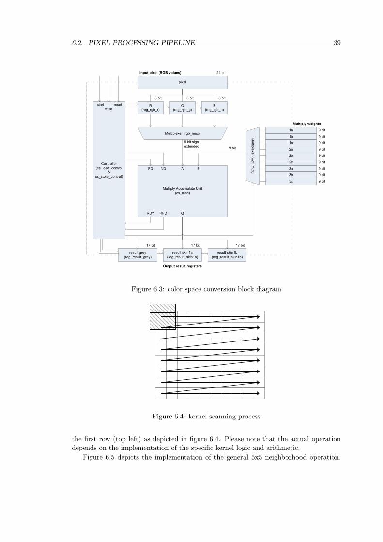
6.2. PIXEL PROCESSING PIPELINE 39
R
(reg_rgb_r)
G
(reg_rgb_g)
B
(reg_rgb_b)
pixel
24 bit
8 bit8 bit8 bit
Multiplexer (rgb_mux)
Multiply Accumulate Unit
(cs_mac)
1a
1b
1c
2a
2b
2c
3a
3b
3c
Multiplexer (w
gt_mux)
A B
Controller
(cs_load_control
&
cs_store_control)
FD ND
RDY RFD Q
result grey
(reg_result_grey)
result skin1a
(reg_result_skin1a)
result skin1b
(reg_result_skin1b)
Input pixel (RGB values)
Multiply weights
start reset
Output result registers
9 bit
9 bit
9 bit
9 bit
9 bit
9 bit
9 bit
9 bit
9 bit
17 bit17 bit17 bit
valid
9 bit sign
extended 9 bit
Figure 6.3: color space conversion block diagram
Figure 6.4: kernel scanning process
the first row (top left) as depicted in figure 6.4. Please note that the actual operationdepends on the implementation of the specific kernel logic and arithmetic.
Figure 6.5 depicts the implementation of the general 5x5 neighborhood operation.

40 CHAPTER 6. IMPLEMENTATION
FIFO
input pixel
output pixel
R
E
G
R
E
G
Controller
read write
input pixel
output pixel
start
input valid
done
output valid
Figure 6.5: general structure of a 5x5 neighborhood operation
To implement the scanning behavior of the kernel window, pixels enter the window atthe bottom right. At the start of each pipeline cycle, all pixels in the window are shiftedone position left. Pixels being shifted outside the kernel window enter the local 4 channelFIFO. After shifting one image row, these pixels are read from the fifo and reenter thekernel window at the right shifted one row upwards. This effectively implements thescanning process as depicted in figure 6.4. Note that since the kernel window logicdepends on the operation implemented, this logic is not shown in this figure.
The controller implements the pipeline protocol handling and additionally controlsthe read and write signals of the FIFO. Initially, the first pixel of an image enters atthe bottom right position of the kernel. However, the output starts whenever the firstpixel is located in the center position of the kernel window. This initial latency has beenimplemented by qualifying the output valid signal with a pixel counter.
The image boundary conditions represent an additional complexity and occur whenthe kernel window should include non-existing ”pixels” outside the actual input image.The implementation should account for these conditions by either replicating the near-est existing pixels or setting the appropriate values to zero. In order to simplify theimplementation it was decided to set these pixel values to zero. This also prevents thealgorithm to detect false results at the border areas.
The binary erosion, dilation and closing operations and the uniform filter and localcount operations are all based on the above window scanning process. The followingsections therefore concentrate on the kernel logic implemented for these operations.

6.2. PIXEL PROCESSING PIPELINE 41
6.2.5 Binary erosion, dilation and closing
For binary erosion and dilation (present in pipeline stage 9), the kernel logic remains quitesimple. The implementation of the dilation operation utilizes the logical OR function ofthe entire neighborhood as shown in equation 6.3.
Output = W11 + W12 + W13 + W14 + W15 + ... + W55 (6.3)
where the pixels in the neighborhood of the input pixel are denoted as W11 for the topleft and W55 for the bottom right. The input pixel is represented with W33.
Similarly, the implementation of the erosion operation uses the logical AND of theentire neighborhood as shown in equation 6.4.
Output = W11 •W12 •W13 •W14 •W15 • ... •W55 (6.4)
where the pixels in the neighborhood of the input pixel are denoted as W11 for the topleft and W55 for the bottom right. The input pixel is represented with W33.
Since the binary closing operation is defined as a binary dilation followed by a binaryerosion, the closing operation (present in pipeline stage 11) is implemented by cascadinginstances of a dilation operation and an erosion operation. Similarly, the implementationof a binary opening operation can be similarly achieved by cascading an erosion operationand a dilation operation.
6.2.6 Convolution filter
The implementation of the convolution filter consists of a 5x5 neighborhood operationwith parameterizable kernel weights. The current implementation is restricted to positivekernel weights of powers2 of 2. The motivation is that in this case the kernel operation canbe simplified to shifting instead of multiplying the pixel values. However, an advancedimplementation using multipliers allows use of arbitrary kernel weights but increases theoperation time and resource utilization.
The structure of the convolution filter kernel implementation is depicted in figure6.6. It was decided to split the operation into three subsequent stages:
1. First stage: neighborhood pixel shifting (multiplication); shifts each neighboringpixel left by the amount of bits specified by the kernel weight. This is depicted inthe figure by kernel window blocks with a pixel value input and a shifting amountinput. The actual shifting process is not shown but is assumed to take place inthese blocks.
2. Second stage: row wise accumulation; accumulates the results of the previous stagein a row wise fashion. The outputs of the kernel window blocks in each row formthe inputs of the row accumulators.
2The current implementation allows for the following kernel weights: 0, 1, 2, 4, 8, 16, 32, 64, 128 and256.

42 CHAPTER 6. IMPLEMENTATION
ACC
ACC
ACC
ACC
ACC
ACC
20 bit
20 bit
20 bit
20 bit
20 bit
shift24 bit 24 bit
16 bit
16 bit
16 bit
16 bit
16 bit
Figure 6.6: (uniform) filter kernel implementation
3. Third stage: column wise accumulation and result shifting; accumulates the resultsof the previous stage and shifts the result right by the amount of bits specified bya configurable parameter. This allows a division of the result by a power of 2.
With this architecture the uniform filter (present in pipeline stage 9) can easily beimplemented by utilizing equal weights throughout the kernel. Furthermore, variousother filter types can be implemented by utilizing different filter weights and shifting theoutput if necessary. For example, an approximate implementation of a gaussian filtermight be achieved by applying the appropriate filter weights.
6.2.7 Local count
The local count operation (present in pipeline stage 7) consists of a 7x7 neighborhoodoperation, its structure is similar to the 5x5 neighborhood operation as discussed insection 6.2.4.
The kernel implementation structure is depicted in figure 6.7 and consists of 7 7-input lookup tables connected to a shared accumulator. The pixels of each window rowform the inputs to the corresponding one count lookup table. This lookup table containsprecalculated one count values for all possible input combinations. Since there are 7inputs, 27 = 128 possible input combinations are encoded in the lookup table. Theoutputs of the lookup tables are subsequently multiplexed into the operand input of theaccumulator. At the end of every processing cycle the accumulator contains the amountof ones present in the neighborhood.

6.2. PIXEL PROCESSING PIPELINE 43
one count
LUT
one count
LUT
one count
LUT
one count
LUT
one count
LUT
one count
LUT
one count
LUT
accumulatormux
3 bit
3 bit
3 bit
3 bit
3 bit
3 bit
3 bit
8 bit
Figure 6.7: local count filter kernel implementation
6.2.8 Remaining operations
The remaining processing blocks (addition/subtraction, multiplication, division andthreshold) will not be discussed in detail since these basically consist of standard math-ematical operations extended with logic required by the pipeline protocol.
The addition, substraction, multiplication and division components are based onfunctionality provided by the Xilinx Core Generator. This utility automatically generatesan efficient implementation of the respective operations in hardware. The thresholdcomponents were similarly realized using standard greater or equal comparators.
The absolute difference component implements equation 3.11. It consists of a sub-tractor with additional operand swapping logic. This logic swaps the input operands ofthe subtractor to guarantee that the first operand always contains the largest operand.Since the operands are positive (both represent grey scale values), the result will bepositive and thus represent the absolute difference between the two operands.
As mentioned in section 6.2.4, the uniform filter, local count and erosion and dila-tion components introduce an initial latency. The pipeline registers in the same stagetherefore also need to introduce the exact same latency to produce synchronized output.This is required to guarantee synchronized output of the different components in eachstage. For this purpose, the delaying pipeline ”register” was developed. This registerconsists of a FIFO to compensate for the initial delay introduced by the componentsmentioned. It only outputs a value if the other components residing in the same pipelinestage produce a valid output.

44 CHAPTER 6. IMPLEMENTATION
Table 6.1: XC2VP30 utilization summary
used total ratio
Slices 12,141 13,696 88%
Slice registers 11,045 27,392 40%
4-input LUTs 17,459 27,392 63%
Block RAM 124 136 91%
6.2.9 Implementation results
The accelerator architecture, the pixel processing pipeline and the image processing com-ponents have been implemented using Xilinx Platform Studio 7.1i and Xilinx IntegratedSoftware Environment 7.1i and synthesized using Xilinx Synthesis Tool. The accel-erator project files, including the PowerPC software source code and pixel processingpipeline VHDL files, can be found on the accompanying CDROM. Appendix E providesan overview of the files on this CDROM.
A summary of the FPGA resources used by the accelerator is shown in table 6.1. Thetotal utilization of the logic resources (slices) is 88% while only 37% are required for theimplementation of the pixel processing pipeline. The remaining resources are used bythe accelerator architecture. The high utilization of block RAM is due to the instructionand data memory space needed for the PowerPC processor. A detailed discussion of theresource utilization of the individual accelerator components is available in appendix D.
6.3 Summary
In the chapter we presented the implementation of both the processor functionality andthe pixel processing pipeline and its components. The implementation method allowsfor modification of the operations in next versions of the algorithm. The parameters ofthe operations can be modified at run-time by updating the parameter registers of thepixel processing pipeline.

System verification andevaluation 7The component implementations as discussed in chapter 6 have been evaluated and testedin order to verify their correctness. This chapter presents the verification and test resultsof these components. First, the test results of the individual components are discussed,then the pixel processing pipeline verification results and the overall system test resultsare presented.
7.1 Image processing components
The image processing components were individually verified before integrating them inthe complete pixel processing pipeline. The verification methodology involved compar-ison of the hardware generated output with software generated output. The simulatedhardware output has been achieved through behavioral simulation1 of the componentsand writing the output to a text file. The software output was generated by implementingthe operations in software using the OpenCV [17] image processing library and writingthe output to a text file. The resulting text files were read by a comparison program andthe differences were written to another text file. The simulation and software outputsand the differences were converted into images to allow visible inspection. The followingsubsections discuss the verification results of the components.
7.1.1 Color space conversion
Figure 7.1 depicts the results from the color space conversion. The source RGB image(a) has been converted to grey scale by software (b) and by simulation of the colorspace conversion component (c) based on equation 3.8. Differences between softwareand hardware simulation are shown in (d). It should be noted that the differences havebeen scaled by a factor of 50 to improve visibility, the grey areas therefore represent adifference in pixel values of 1 between the hardware and the software.
The figure shows that in certain areas differences are present. These differences canbe attributed to the error in the calculation method utilized by the color space conversioncomponent. For grey scale conversion the following calculation is performed:
Grey =R ∗ 85 + G ∗ 85 + B ∗ 85
256(7.1)
where Grey is the resulting grey scale output, R, G and B represent the input pixel colorcomponents. The grey scale conversion averages the color components by multiplying
1Using a hardware description language, components are developed by describing their behavior atthe level of clock cycles. Simulation at this level is denoted behavioral simulation. We used the ModelsimSE 6.0a software package for behavioral simulation.
45

46 CHAPTER 7. SYSTEM VERIFICATION AND EVALUATION
ba
dc
Figure 7.1: color space conversion results; original (a), software output (b), hardwaresimulation output (c) and difference between software and hardware (d)
each component with a factor of 1/3. In our implementation we approximated this factorby using a factor of 85/256 ≈ 1/3. First, the individual color components (R, G, andB) are multiplied by 85 and the results are accumulated. Then, an 8 bit right shiftoperation, which corresponds to a division by 256, is performed to yield the grey scaleconversion result Grey. It can therefore be seen that the result is an approximation withthe following error factor:
∆E = 1− 3 ∗ 85256
=1
256(7.2)
where ∆E is the error factor. This error factor becomes notable in the higher intensityareas of the image as can be seen in figure 7.1(d). The error in higher intensities is largerand thus results in differences because of truncation in hardware.
7.1.2 Binary dilation, erosion and closing
The dilation, erosion and closing components have been tested using a binary inputimage. Figures 7.2, 7.3 and 7.4 depict the respective simulation results. The inputimages are depicted in (a), the software generated outputs in (b), the hardware simulationoutputs in (c) and the differences between the software output and simulation outputare depicted in the (d) sections of these figures.
The dilation results in figure 7.2 do not show differences between the software outputand the hardware output. We can therefore conclude that the hardware produces the

7.1. IMAGE PROCESSING COMPONENTS 47
a b
c d
Figure 7.2: binary dilation results; original (a), software output (b), hardware simulationoutput (c) and difference between software and hardware (d)
correct results.The erosion results in figure 7.3 do not show differences between the software output
and the hardware output. However, as mentioned in section 6.2.4, the PPP componentsassume a value of 0 at the image borders whereas software algorithms often replicate thenearest border pixels. This might result in differences between the software output andthe hardware output. It occurs in the closing results depicted in figure 7.4. Since the im-plementation of the erosion consists of the logical AND of all pixels in the neighborhood,it will always generate output of zero at the border areas. The software output howeverreplicates the border pixels and thus generates a white output at the border areas. Forour application we consider this acceptable since the border areas of the input image areof less interest.
7.1.3 Uniform filter
The implementation of the uniform filter was generalized into a convolution operationfor 8 bit pixel values with a configurable 5x5 kernel. Our implementation of the uniformfilter uses weights of 1. The results of the simulation are shown in the figure 7.5.
Apart from the border areas, the hardware simulation produces correct output. Thedifferences shown in (d) between the hardware simulation output (c) and the softwaregenerated output (b) indicates differences in the border areas of the image. The reasoncan be attributed to the fact that the PPP component handles the border situationsdifferently. Whereas the software algorithm replicates the input pixel values outside the

48 CHAPTER 7. SYSTEM VERIFICATION AND EVALUATION
a b
c d
Figure 7.3: binary erosion results; original (a), software output (b), hardware simulationoutput (c) and difference between software and hardware (d)
a b
c d
Figure 7.4: binary closing results; original (a), software output (b), hardware simulationoutput (c) and difference between software and hardware (d)

7.1. IMAGE PROCESSING COMPONENTS 49
a b
c d
Figure 7.5: uniform filter results; original (a), software output (b), hardware simulationoutput (c) and difference between software and hardware (d)
borders, the PPP component sets these values to 0.
7.1.4 Local count
Simulation results for the local count operation are depicted in figure 7.6. The outputof both software (b) and hardware simulation (c) have been increased by a factor of 5 inorder to aid visibility.
Apart from the border areas, the hardware simulation produces correct output. Alsofor this component the border areas differ with the software implementation because ofthe fact that the component assumes values of 0 near these boundaries. In our imple-mentation this results in darker borders in the output image.
7.1.5 Remaining operations
The simulation results for the threshold operation can be found in figure 7.7. Thethreshold value was set to 200, the results show that the hardware simulation (c) producesoutput identical to the software implementation (b) since there are no differences visiblein (d).
The remaining operations present in the PPP have been verified through testing ofall possible input combinations. With the exception of the division component, all com-ponents generate flawless results. The division component results in minor truncationerrors because of the fixed size of the fractional remainder. Since the implementation

50 CHAPTER 7. SYSTEM VERIFICATION AND EVALUATION
a b
c d
Figure 7.6: local count results; original (a), software output (b), hardware simulationoutput (c) and difference between software and hardware (d)
a b
c d
Figure 7.7: threshold results; original (a), software output (b), hardware simulationoutput (c) and difference between software and hardware (d)

7.2. PIXEL PROCESSING PIPELINE 51
a b
c d
Figure 7.8: pixel processing pipeline skin segmentation results; original (a), softwareoutput (b), hardware simulation output (c) and difference between software and hardware(d)
uses 8 bits for the fractional remainder, the maximum error in the remainder is 2−8.Increasing the amount of bits for the remainder would decrease the maximum error.However, the throughput will be lower since the computation of the remainder thenrequires more clock cycles.
7.2 Pixel Processing Pipeline
The implementation of the pixel processing pipeline comprises the components as dis-cussed in section 6.2.1. After integrating these components, a manual stage by stageverification using behavioral simulation was performed. Then the simulation of process-ing a complete input image was performed. The verification results of this simulation aredepicted in figure 7.8. The source image is shown in (a), the software generated outputin (b) and the hardware simulation output in (c).
The difference comparison (d) shows that in certain cases the skin segmentationfrom the PPP differs in the output generated by the software. The differences can beattributed to the fact that the color space conversion and division components containa fixed precision which introduce minor truncation errors in the conversion weights.

52 CHAPTER 7. SYSTEM VERIFICATION AND EVALUATION
ppp_software_excel Grafiek 1
Page 1
0
20
40
60
80
100
120
1 3 5 7 9 11 13 15 17 19 21 23 25 27 29 31 33 35 37 39 41 43 45 47 49 51 53 55 57 59 61
t (s)
%
0
5
10
15
20
25
30
fps CPU utilization in %
Framerate (frames per second)
Figure 7.9: Software algorithm performance
7.3 Integral system performance evaluation
To perform integral system testing we used a stand alone workstation based on a 2,8 GHzPentium 4 processor with 1024MB memory running Windows XP Pro as our referenceand measurement system. The system setup additionally consists of a Philips ToUCamPro webcam.
First the performance of the algorithm software implementation was estimated. Fig-ure 7.9 shows both the CPU utilization and the achieved frame rate. As can be observedfrom the measurements, the software version is unable to achieve the real-time perfor-mance criterion of 25 frames per second. It achieves a frame rate close to 14 frames persecond at a CPU utilization rate of 100%.
Figure 7.10 shows the results of the application demonstrator utilizing the hardwareaccelerator. The CPU utilization rate varies between 60% to 70% while the frame rateremains steady around 20 fps. This is a considerable improvement compared to thesoftware version since the CPU utilization rate is significantly lower while yielding ahigher frame rate. However, the real-time performance criterion of 25 frames per secondis not met in the current implementation. Since the CPU utilization is not yet at 100%,the cause of the bottleneck remains in the network communication. However, the exactcause remains to be investigated.
The frame rate speedup gained with our hardware accelerated implementation is20/14 ≈ 1.43. Moreover, the CPU utilization is 30% to 40% lower compared to thesoftware implementation using the same computing system. Thus it allows for higherlevel applications such as hand gesture recognition to process the skin segmented output.
Future research needs to be performed to identify the exact network bottleneck of thecurrent implementation which limits the achieved frame rate to 20 frames per second.

7.4. CONCLUSION 53
ppp_hardware_excel Grafiek 1
Page 1
0
20
40
60
80
100
120
1 3 5 7 9 11 13 15 17 19 21 23 25 27 29 31 33 35 37 39 41 43 45 47 49 51 53 55 57 59 61
t(s)
%
0
5
10
15
20
25
30
fps
CPU utilization in %
Packet Loss in %
Framerate (frames per second)
Figure 7.10: Hardware implementation performance
7.4 Conclusion
The evaluation as presented in this chapter shows the correct operation of the differentcomponents involved in the proposed accelerator system. Through behavioral simula-tion and testing of the implemented components and the pixel processing pipeline weverified that the skin segmentation algorithm has been successfully implemented in hard-ware. A demonstration system setup shows that the accelerator achieves a speedup ofapproximately 1.43 compared to its software implementation. Moreover, the CPU uti-lization rate was reduced from 100% to approximately 60% to 70%. Future work shouldconcentrate on increasing the achieved frame rate and image sizes.

54 CHAPTER 7. SYSTEM VERIFICATION AND EVALUATION

Conclusions and Future Work 8This chapter concludes the discussion of this thesis project and provides suggestions forpossible future work.
8.1 Conclusions
This project focused on the design and implementation of an FPGA accelerator forreal-time skin segmentation. This report discussed the architectural exploration, design,verification and evaluation of both the accelerator architecture and its components.
We implemented the skin segmentation algorithm in hardware in order to meet thereal-time requirements of 25 frames per second at an image resolution of at least 320x240pixels. The demonstrator developed during this project achieves a frame rate of only20 frames per second and a resolution of 320x240 pixels. The speedup gained with ourhardware accelerated implementation is 1.43. Moreover, the CPU utilization is 30% to40% lower compared to the software implementation using the same computing system.Thus it allows other software layers such as hand gesture recognition to more exactlyinterpret the skin segmented output.
Our design utilizes approximately 88% of the resources available in the XC2VP30FPGA. Only 37% are required by the implementation of the pixel processing pipeline,the remaining resources are used by the accelerator architecture. The PowerPC processoroperates at a clock frequency of 300 MHz while the pixel processing pipeline operates ata clock frequency of 100 MHz.
Besides the speedup mentioned above, our accelerator provides a portable solutiondue to the used standard network interface. This allows our accelerator to be used witha wide range of host PC’s (both desktops and laptops).
8.2 Future work
Future work on this accelerator should concentrate on reducing the packet loss andthe communication overhead. Furthermore, the design could also be implemented on agigabit ethernet platform (such as presented in [13]) to achieve an input video resolutionof 640x480 pixels at a frame rate of 25 frames per second.
It should be noted that the hardware demonstration application has not yet beenoptimized for execution speed. Several optimizations related to network protocol han-dling (as mentioned in amongst others [5], [10] and [16] ) may be employed to reduce thecommunication overhead currently present within the demonstration application. Fur-thermore, research on possible network bottlenecks need be done to increase the framerate of 20 frames per second to at least 25 frames per second.
55

56 CHAPTER 8. CONCLUSIONS AND FUTURE WORK
A (simple) data compression algorithm can be employed to reduce the required net-work bandwidth. The overhead of such algorithm can be handled by the second PowerPCprocessor present in the FPGA. Furthermore, the following items specifically related tothe pixel processing pipeline may be addressed in the future:
• Utilization of a higher clock frequency for the pixel processing pipeline. Currently,a clock frequency of 100 MHz is employed since this frequency is also used for thePLB bus. Higher clock frequencies might be possible but require specific designconsiderations regarding the interface with the PLB bus.
• The color space conversion component has been implemented with a sharedmultiply-accumulator unit to save FPGA resources. It is desirable to remove thissharing by instantiating three multiply-accumulator units to improve the through-put of the color space conversion component.
• Implementation of a ”start of frame synchronization” for the local operations (uni-form filter, local count, dilation and closing) present in the pipeline. When a pixelpacket is lost during transmission, the entire image line will be lost and thus willnot be processed by the pixel processing pipeline. The local operations howeverassume that all pixel packets arrive consecutively in order to determine when theimage boundaries have been reached. When a packet is lost the internal counterswill incorrectly determine when the image boundaries have been reached. Thusthe local operations need to detect the start of a new frame to ’reset’ their internalimage boundary detection counters.

Bibliography
[1] S. Ahmad, A usable real-time 3d hand tracker, Proceedings of the Conference Recordof the Twenty-Eighth Asilomar Conference on Signals, Systems and Computers(1994), 1257–1261.
[2] A. Argyros and M. Lourakis, Real-time tracking of multiple skin-colored objects witha possibly moving camera, Lecture Notes in Computer Science 3023 (2004), 368–379.
[3] A. Benedetti and P. Perona, Real-time 2-d feature detection on a reconfigurablecomputer, Proceedings of the IEEE Computer Society Conference on ComputerVision and Pattern Recognition (1998).
[4] J.A. Boluda, F. Pardo, F. Blasco, and J. Pelechano, A pipelined reconfigurable ar-chitecture for visual-based navigation, Proceedings of the 25th EUROMICRO Con-ference (1999).
[5] J.S. Chase, A.J. Gallatin, and K.G Yocum, End system optimizations for high-speedtcp, IEEE Communications Magazine 39 (2001), 68–74.
[6] IBM Corporation, Processor local bus architecture specification, version 4.6 (2004).
[7] D. Crookes, K. Benkrid, A. Bouridane, K. Alotaibi, and A. Benkrid, Design and im-plementation of a high level programming environmentfor fpga-based image process-ing, IEE Proceedings Vision, Image and Signal Processing 147 (2000), 377–384.
[8] R. Duncan, A survey of parallel computer architectures, Computer 23 (1990), no. 2,5–16.
[9] M. Flynn, Some computer organizations and their effectiveness, IEEE Transactionson Computing C-21 (1972), 94.
[10] A. Foong, T. Huff, H. Hum, J. Patwardhan, and G. Regnier, Tcp performance re-visited, Proceedings of the International Symposium on Performance Analysis ofSystems and Software (2003).
[11] R. Gonzales and R. Woods, Digital image processing, second ed., Prentice Hall,2002.
[12] A. Grama, Introduction to parallel computing, second ed., Addison Wesley, 2003.
[13] Xilinx System Engineering Group, Gigabit system reference design, Xilinx Applica-tion Note XAPP536 (2004).
[14] , Xilinx university program virtex-ii pro development system, Hardware Ref-erence Manual (2005).
57
58 BIBLIOGRAPHY
[15] J.L. Hennessy and D.A. Patterson, Computer architecture - a quantitative approach,third ed., Morgan Kaufmann Publishers, 2003.
[16] J. Huang and C. Chen, On performance measurements of tcp/ip and its devicedriver, Proceedings of the 17th Conference on Local Computer Networks (1992),586–575.
[17] Intel, Open source computer vision library.
[18] R. Kjeldsen and J. Kender, Finding skin in color images, (1996), 312.
[19] M. Kolsch and M. Turk, Fast 2d hand tracking with flocks of features and multi-cueintegration, 10 (2004), 158.
[20] P. Lam and S. Liew, Udp-liter: An improved udp protocol for real-time multimediaapplications over wireless links, Proceedings of the 1st International Symposium onWireless Communication Systems (2004), 314–318.
[21] L. Larzon, M. Degermark, S. Pink, L. Jonsson, and G. Fairhurst, The lightweightuser datagram protocol (udp-lite), Internet proposed standard RFC 3828 (2004).
[22] J.F. Lichtenauer, E.A. Hendriks, and M.J.T. Reijnders, Robust skin color detectionby elliptic cylinder fitting, BMVC 2006 (submitted for publication).
[23] P. Mc Curry, F. Morgan, and L. Kilmartin, Xilinx fpga implementation of a pixelprocessor for object detection applications, Celoxica application note (2001).
[24] W. Najjar, B. Draper, A.P.W. Bhm, and R. Beveridge, The cameron project: High-level programming of image processing applications on reconfigurable computing ma-chines, Proceedings of the Workshop on Reconfigurable Computing (PACT), Paris(1998).
[25] J. Postel, User datagram protocol, Internet standard RFC 768 (1980).
[26] , Transmission control protocol, Internet standard RFC 793 (1981).
[27] W. Stechele, L. Alvado Crcel, S. Herrmann, and J. Lidn Simn, A coprocessor foraccelerating visual information processing, Proceedings of the Design, Automationand Test in Europe Conference and Exhibition (2005).
[28] Miguel A. Vega-Rodrguez, Juan M. Snchez-Prez, and Juan A. Gmez-Pulido, Realtime image processing with reconfigurable hardware, Proceedings of the 8th IEEEInternational Conference on Electronics, Circuits and Systems, 2001. ICECS 2001.(2001), 213–216.
[29] Xilinx, Virtex-ii pro and virtex-ii pro x platform fpgas: Complete data sheet, version4.5 (2005).
[30] Xilinx Corporation, 2100 Logic Drive,San Jose, CA, Powerpc processor referenceguide, embedded development kit (edk) 6.1 ed., september 2003, version 1.1.

BIBLIOGRAPHY 59
[31] H. Zimmermann, Osi reference model–the iso model of architecture for open systemsinterconnection, IEEE Transactions on Communications 28 (1980), 425–432.

60 BIBLIOGRAPHY

Skin segmentation algorithm AOne of the first stages involved in the current gesture recognition system consists ofidentifying the image regions containing skin colors. This process is denoted ”skin seg-mentation”. The algorithm employed in this project is proposed in [22] and can de-scribed as depicted in figure A.1. The algorithm in this figure is annotated with thebasic mathematical operations involved in each stage of the algorithm.
The algorithm produces an absolute difference output (for change detection) and askin segmented output (for hand gesture recognition). In figure A.1, the left ”branch”denotes the operations required to produce the absolute difference output, the middle andright ”branches” denote the operations required to produce to skin segmented output.The following paragraphs discuss the change detection and skin segmentation parts ofthe algorithm. The numbers indicated correspond to the components in figure A.1.
A.1 Change detection
The algorithm provides an indication of change between two consecutive video frames.This is accomplished by calculating the absolute difference between the frames on a pixelby pixel basis. First, the input RGB pixel is converted to a grey scale pixel (1). Then theabsolute difference between two corresponding pixels in consecutive frames is calculated(14). This can be accomplished by buffering the pixels in an image buffer (11). Theresulting absolute difference image is smoothed using a uniform filter (16). A threshold(18) is applied to the smoothed image with which the sensitivity of the change detectioncan be regulated.
A.2 Skin segmentation
The skin model consists of two components, these are calculated using two color spaceconversions (2, 3). From each component a corresponding mean value is subtracted (4,5). The results are then squared (7, 8) and added (9) to form a density compensateddissimilarity value. The grey value of the input pixel is also squared (6) before it divides(10) the density compensated dissimilarity. The result provides an indication of the skinlikelihood and is thresholded using two different threshold values (12, 13). The secondthreshold (13) output is processed with a local count filter (15) followed by a threshold(17). This effectively filters the output of (13) of small regions. It is processed usinga dilation (19) to thicken the contours of the resulting areas of (17). The logical ANDfunction of the dilation (19) result and the first threshold (12) is then processed with aclosing (20) operation to yield the skin segmented output.
61

62 APPENDIX A. SKIN SEGMENTATION ALGORITHM
color space
conversion
color space
conversion
mult + add + shift mult + add + shift
color space
conversion
mult + add + shift
mean subtract
add
mean subtract
add
square
mult
square
mult
square
mult
Grey level value
Size 8 bits
Range (0, 255)
First component skin model 1
Size 9 bits
Range (0, ±255)
Second component skin model 1
Size 9 bits
Range (0, ±255)
Corrected first component
Size 10 bits
Range (0, ±512)
Corrected second component
Size 10 bits
Range (0, ±512)
Mean 2
Size 9 bits
Range (0, ±255)
Mean 1
Size 9 bits
Range (0, ±255)
Squared first component
Size 19 bits, always positive
Range (0, 5122)
Squared second component
Size 19 bits, always positive
Range (0, 5122)
dissimilarity
add
Density compensated dissimilarity
Size 19 bits (discard input sign bits)
Range (0, 5122)
When 0 then set to 1
Squared grey value
Size 17 bits, always positive
Range (0, 2552)
When 0 set to 1
division
mult + add
RGB pixel, 24 bit
thresholding
comp
Threshold value
Size 26 bits
Range (0, ±2*2553)
Division result (quotient, fractional remainder)
Size 26 bits
Range (0, ±2*2553)
thresholding
comp
Threshold value
Size 26 bits
Range (0, ±2*2553)
Thresholded value
Size 1 bit
Thresholded value
Size 1 bit
image buffer
absolute
difference
comp + add
Grey value previous frame
Size 8 bits
Range (0, 255)
uniform filter(conv5)
mult + add + shift
Absolute difference
Size 8 bits
Range (0, 255)
Local change intensity
Size 8 bits
Range (0, 255)
thresholding
comp
Threshold value
Size 8 bits
Range (0, 255)
Local change intensity
Size 1 bit
Convolution weights
Size 8 bits
Range (0, 255)
local count(conv7)
count + shift
thresholding
comp
Threshold value
Size 6 bits
Range (0, 49)
Local count
Size 6 bits
Range (0, 7*7=49)
dilation
comp + shift
Size 1 bit
closing
comp + shift
and
Dilated
Size 1 bit
Dilated
Size 1 bit
Conversion weights (3)
Size 9 bits
Range (0, ±255)
Conversion weights (3)
Size 9 bits
Range (0, ±255)
Conversion weights (3)
Size 9 bits
Range (0, ±255)
1 2 3
4 5
6 7 8
9
10
11 12 13
14 15
16 17
18 19
20
Figure A.1: skin segmentation algorithm
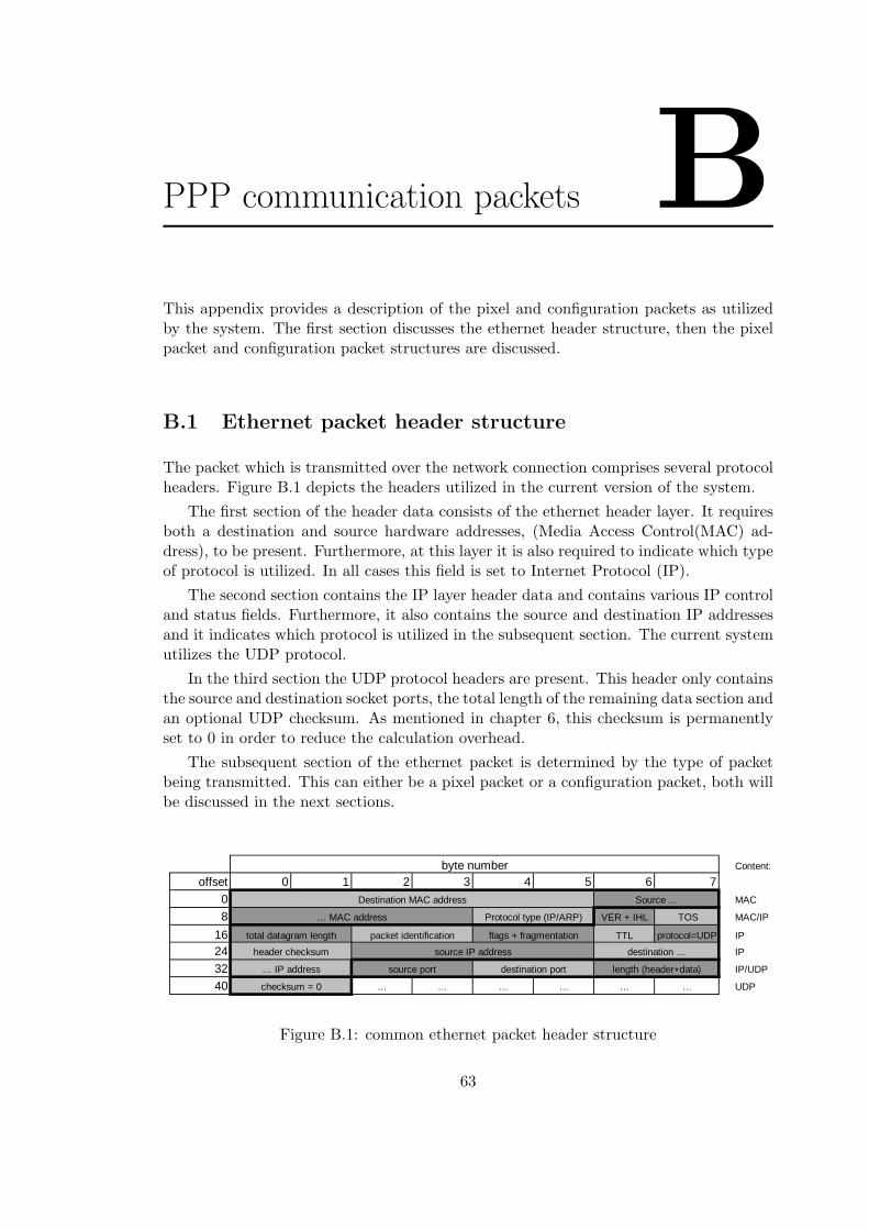
PPP communication packets BThis appendix provides a description of the pixel and configuration packets as utilizedby the system. The first section discusses the ethernet header structure, then the pixelpacket and configuration packet structures are discussed.
B.1 Ethernet packet header structure
The packet which is transmitted over the network connection comprises several protocolheaders. Figure B.1 depicts the headers utilized in the current version of the system.
The first section of the header data consists of the ethernet header layer. It requiresboth a destination and source hardware addresses, (Media Access Control(MAC) ad-dress), to be present. Furthermore, at this layer it is also required to indicate which typeof protocol is utilized. In all cases this field is set to Internet Protocol (IP).
The second section contains the IP layer header data and contains various IP controland status fields. Furthermore, it also contains the source and destination IP addressesand it indicates which protocol is utilized in the subsequent section. The current systemutilizes the UDP protocol.
In the third section the UDP protocol headers are present. This header only containsthe source and destination socket ports, the total length of the remaining data section andan optional UDP checksum. As mentioned in chapter 6, this checksum is permanentlyset to 0 in order to reduce the calculation overhead.
The subsequent section of the ethernet packet is determined by the type of packetbeing transmitted. This can either be a pixel packet or a configuration packet, both willbe discussed in the next sections.
Content:
offset 0 1 2 3 4 5 6 7
0 MAC
8 VER + IHL TOS MAC/IP
16 TTL protocol=UDP IP
24 IP
32 IP/UDP
40 … … … … … … UDP
byte number
Destination MAC address Source …
… MAC address Protocol type (IP/ARP)
total datagram length packet identification flags + fragmentation
header checksum source IP address
checksum = 0
destination …
… IP address source port destination port length (header+data)
Figure B.1: common ethernet packet header structure
63

64 APPENDIX B. PPP COMMUNICATION PACKETS
40 IP/-
48 -
56 -
64 0xFF type = 0x01 camera reserved 0XFF reserved accelerator
72 0xFF reserved 0xFF reserved accelerator
80 pixel data
|
240
checksum = 0
reserved
frame number
column number (x)line number (y)
reserved
reserved
pixel data
Figure B.2: pixel packet header structure
B.2 Pixel packet structure
Pixels are communicated using pixel packets as depicted in figure B.2. The indicatedchecksum field belongs to the UDP section of the packet.
The first 24 bytes are reserved in order to align the start of the pixel data at a 64 bitoffset address. This requirement is posed by the PLB bus DMA protocol [6].
Then the PPP packet type is indicated, a pixel packet is indicate using type 1. Thecamera ID indicates which camera this pixel packet belongs to. The frame numbercontains the sequence number of the frame to which the pixels belongs to. The linenumber and column number indicate the x and y coordinates of the first pixel presentwithin the pixel data section. Reserved bytes are also present within the packet to allowa modified implementation of the header in the future.
The pixel data can either contain input pixels (transferred from the host PC to theaccelerator) or output pixels (transferred from the accelerator to the host PC). The inputpixels are represented as depicted in the following table.
Grey T−1 Blue Green Red
Table B.1: Input pixel format
where Grey T−1 represents the grey value of the corresponding pixel in the previousframe, Blue, Green and Red represent the blue, green and red color components of theinput pixel.
The output pixels are represented as depicted in the following table.
0 Change Grey T Skin
Table B.2: Output pixel format
where Change represents the change estimation of the processed pixel, Grey T representsthe grey value of the processed pixel and Skin represent the skin segmented output ofthe processed pixel. The empty (zero) field was added to ensure that the output pixelpackets have the same size as the input pixel packets. This simplifies the software onboth the PowerPC processor and the host PC.

B.3. CONFIGURATION PACKET STRUCTURE 65
40 IP/-
48 -
56 -
64 0xFF type = 0x02 accelerator
72 parameters
80 parameters
88 parameters
96 uni w23 uni w22 uni w21 uni w15 uni w14 uni w13 uni w12 uni w11 parameters
104 uni w41 uni w35 uni w34 uni w33 uni w32 uni w31 uni w25 uni w24 parameters
112 uni w54 uni w53 uni w52 uni w51 uni w45 uni w44 uni w43 uni w42 parameters
120 uni shift uni w55 parameters
128 divt2 remd divt1 remd parameters
136 parameters
144 -
|240
reservedchecksum = 0
weight skin 1aR
reserved
reserved
reserved
weight grey Rweight grey Gweight grey Breserved
reserved
reserved weight skin1aB weight skin1aG
reserved
reserved
division threshold 1 quotientdivision threshold 2 quotient (lccnt)
local count thresholduniform filter threshold
weight skin1bRweight skin1bGweight skin1bB
Figure B.3: configuration packet header structure
B.3 Configuration packet structure
The structure of a configuration packet is depicted in figure B.3. To indicate that thepacket contains configuration data, the type field should be set to 2. The subsequentthree section then contain the color space conversion weights. Currently the implemen-tation allows for 9 bit signed conversion weights.
The uniform filter weights are presented using a single byte per weight. Each weightindicates either a multiplication factor of zero (0) or a shift left value (1-8) for the uniformfilter kernel operation. The uni shift value indicates the amount of bits the result of thekernel operation should be shifted right.
Two division threshold values are present: the threshold value required before thelocal count (threshold 2 lccnt) operation and the threshold value which is directly con-nected to the AND port before the closing operation. Both threshold values consist of aninteger quotient part and an 8-bit fractional remainder part. This remainder thereforeprovides an accuracy of 1/256th.
Both uniform threshold value and local count threshold value are present at the endof the configuration data packet.

66 APPENDIX B. PPP COMMUNICATION PACKETS

PPP slave registers CThe pixel processing pipeline contains 16 slave registers which are directly addressableby the processor. These registers are used as programmable parameters of the pipelinecomponents an can be changed during run-time by sending configuration packets from thehost PC to the system. Figure C.1 provides an overview of the currently employed slaveregisters and their respective function. The organization corresponds to the structure ofthe configuration packet structure as discussed in appendix B.
mean 2 mean 1
skin1a3skin1b3 skin1b2 skin1b1
conv5_w24conv5_w25conv5_w31conv5_w32
63
grey1agrey1bgrey1c
47485556 2324lower
323940upper
078151631
conv5_w11conv5_w12conv5_w13conv5_w14
skin1a1skin1a2
conv5_w22conv5_w23 conv5_w15conv5_w21conv5_w33conv5_w34conv5_w35conv5_w41
conv5_w54shamt conv5_w55
conv5_w51conv5_w52conv5_w53 conv5_w42conv5_w43conv5_w44conv5_w45
div tr1_remddivision threshold 1div tr2_remddivision threshold 2 (to local count)uniform filter threshold local count threshold
Figure C.1: PPP slave register organization
The following table provides an overview of the parameters, their function, range anddefault values.
67

68 APPENDIX C. PPP SLAVE REGISTERS
Parametername
Description Range Defaultvalue
grey1a Grey scale conversion weight for the redcolor component
0 - +255 85
grey1b Grey scale conversion weight for thegreen color component
0 - +255 85
grey1c Grey scale conversion weight for theblue color component
0 - +255 85
skin1a1 Skin model 1a conversion weight for thered color component
-256 -+255
-61
skin1a2 Skin model 1a conversion weight for thegreen color component
-256 -+255
245
skin1a3 Skin model 1a conversion weight for theblue color component
-256 -+255
-185
skin1b1 Skin model 1b conversion weight for thered color component
-256 -+255
50
skin1b2 Skin model 1b conversion weight for thegreen color component
-256 -+255
-120
skin1b3 Skin model 1b conversion weight for theblue color component
-256 -+255
-162
conv5 w11 Uniform filter shifting weight 1,1 (topleft)
0 - 256 1
conv5 w12 Uniform filter shifting weight 1,2 0 - 256 1conv5 w13 Uniform filter shifting weight 1,3 0 - 256 1conv5 w14 Uniform filter shifting weight 1,4 0 - 256 1conv5 w15 Uniform filter shifting weight 1,5 (top
right)0 - 256 1
conv5 w21 Uniform filter shifting weight 2,1 0 - 256 1...
conv5 w55 Uniform filter shifting weight 5,5 (bot-tom right)
1 - 256 1
shamt Uniform filter result shift right amount 0 - 8 0mean1 Mean subtract value for skin1a1 -256 -
+255-30
mean2 Mean subtract value for skin1a2 -256 -+255
-6
divisionthreshold1
Division quotient threshold to AND 0 - 65536 0
div tr1 remd Division fractional remainder thresholdto AND
0 - 255 4
divisionthreshold2
Division quotient threshold to localcount
0 - 65536 0
div tr2 remd Division fractional remainder thresholdto local count
0 - 255 1
local countthreshold
Threshold after local count 0 - 65536 15
uniform filterthreshold
Threshold after uniform filter 0 - 65536 1250(50*25)
Table C.1: PPP Parameter Descriptions

Implementation data DThis appendix describes the implementation results which provide insights into the re-source utilization and timing of the individual pixel processing pipeline components. Weimplemented the accelerator architecture and its components using the Xilinx PlatformStudio version 7.1i and the Xilinx Integrated Software Environment 7.1i. The synthesistool used was Xilinx Synthesis Tool (XST) version 7.1.02i H.42.
The Virtex 2 Pro FPGA contains an array of interconnected Configurable LogicBlocks (CLB’s). Each CLB contains 4 slices and 2 tri-state buffers. The slices areequivalent and contain amongst others 2 function generators and 2 storage elements.The function generators can be configured as either 4-input Lookup-Tables (LUTs), 16-bit shift registers or 16 bit Random Access Memory (RAM). The storage elements canbe configured as D-type flip flops or level sensitive latches. The FPGA also containsBlock RAM elements which can be used as dual port RAM.
The following tables present implementation details of the accelerator, pixel process-ing pipeline and the individual image processing components. The amount of finite statemachines (FMSs), adders/subtractors and look-up tables indicated in these tables areresults gained from HDL synthesis and do not necessarily present the low level synthesisresults. The presented results assume an implementation with input image parametersof 320 width and 240 height. The resource utilization details for a 640x480 implementa-tion are similar, the initial delay figures however differ. Resource utilization percentagesindicate the utilization of the Virtex 2 Pro-30 [29] FPGA used in our implementationplatform.
Accelerator systemResource utilizationSlices 12138 (88%)Flip Flops 11045 (40%)4-input LUTs 17462 (63%)Block RAM 124 (91%)Multipliers 4 (2%)
Table D.1: implementation metrics for accelerator system
Table D.1 shows that the accelerator system uses 88% of the available slices and40% of the available flip flops. Approximately 63% of the occupied slices are used as4-input LUTs. Furthermore, the accelerator uses 91% of the available Block RAM, themajority of which can be attributed to both instruction and data memory required by thePowerPC processor. The current implementation requires 64 KB of instruction memoryand 128 KB of data memory. Since a single Block RAM can contain a maximum of
69

70 APPENDIX D. IMPLEMENTATION DATA
2,25 KB [29], the amount of Block RAM resources used by the PowerPC memories is(128 + 64)/2, 25 ≈ 86.
Pixel Processing PipelineResource utilizationSlices 5201 (37%)Flip Flops 5751 (20%)4-input LUTs 9096 (33%)Block RAM 21 (15%)HDL SynthesisFSMs 32ROMs 111Adders/Subtractors 29Counters 15Accumulators 2Registers 2017Latches 1Comparators 16Multiplexers 178Logic shifters 2Xors 96
Table D.2: implementation metrics for pixel processing pipeline
Table D.2 summarizes the resource utilization of the pixel processing pipeline. Ap-proximately 37% of the available slices, 20% of the flip flops and 33% of the LUTs areused by the pixel processing pipeline. Furthermore, 15% of the available Block RAM isused.
The HDL synthesis results indicate the logic components involved in the pixel process-ing pipeline. It shows that 32 Finite State Machines (FSMs) have been inferred. TheseFSMs result from VHDL processes often performing a controlling function. The tableshows that 111 ROMs have been synthesized, these are inferred from fixed lookup struc-tures. Furthermore, 29 Adders/Subtractors, 15 Counters and 2 Accumulators have beeninferred. Along with the 16 Comparators, these are often involved in supporting theFSMs.
Table D.3 shows the implementation and timing details of the local count component.The timing details show that this component requires 11 clock cycles to complete itsoperation. Consequently, the local count will produce an output 11 clock cycles afterthe start of a new pipeline cycle. However, this will not be the case during the firstpipeline cycles. The initial delay indicates that initially 964 pipeline cycles with validinput to the component must occur before valid output is produced. This initial delay istypical for all components based on the neighborhood operation principle as explainedin section 6.2.4. The reason is that these components must shift several image lines intotheir internal buffers before being able to calculate an output value.
The table also indicates that several Logicores are used in the design. These Intel-lectual Property (IP) cores are library components developed by Xilinx which can be

71
7x7 local countTimingRequired clock cycles 11Initial latency 964Resource utilizationSlices 415 (3%)Flip Flops 215 (0%)4-input LUTs 792 (2%)BRAMs 1 (0%)HDL SynthesisFSMs 1ROMs 7Adders/Subtracters 1Counters 2Registers 71Multiplexers 1LogicoresAccumulatorEqual comparatorGreater Equal comparatorFIFO
Table D.3: timing and implementation metrics for 7x7 local count component
used as a black box component in the design. In this case, the component consists ofan Accumulator (accumulating subsequent input values), Equal Comparator (comparestwo inputs and sets its output when these are equal), Greater Equal Comparator andFirst In First Out (FIFO) buffer.
For the following tables, the resource utilization, HDL synthesis results and the timingand Logicore details will not be explained further since these can be explained similarlyto the discussions above.

72 APPENDIX D. IMPLEMENTATION DATA
Absolute differenceTimingRequired clock cycles 4Initial latency 0Resource utilizationSlices 46 (0%)Flip Flops 53 (0%)4-input LUTs 65 (0%)HDL SynthesisFSMs 1Registers 10LogicoresGreater Equal comparatorAdder/Subtractor
Table D.4: timing and implementation metrics for absolute difference component
Binary closingTimingRequired clock cycles 3Initial latency 1286Resource utilizationSlices 334 (2%)Flip Flops 260 (0%)4-input LUTs 627 (2%)HDL SynthesisFSMs 2Adders/Subtracters 2Counters 4Registers 70Multiplexers 2LogicoresnoneComponentsErosion/Dilation (2x)
Table D.5: timing and implementation metrics for binary closing component

73
5x5 uniform filterTimingRequired clock cycles 9Initial latency 645Resource utilizationSlices 1751 (12%)Flip Flops 1156 (4%)4-input LUTs 3253 (11%)BRAMs 2 (1%)HDL SynthesisFSMs 3Adders/Subtracters 1Counters 2Registers 110Multiplexers 2LogicoresAccumulator (2x)Equal comparatorGreater Equal comparatorFIFO
Table D.6: timing and implementation metrics for 5x5 uniform filter component
color space conversionTimingRequired clock cycles 21Initial latency 0Resource utilizationSlices 109 (0%)Flip Flops 117 (0%)4-input LUTs 175 (0%)HDL SynthesisFSMs 2Registers 20Multiplexers 2LogicoresMultiply accumulator
Table D.7: timing and implementation metrics for color space conversion component

74 APPENDIX D. IMPLEMENTATION DATA
erosion/dilationTimingRequired clock cycles 3Initial latency 643Resource utilizationSlices 237 (1%)Flip Flops 162 (0%)4-input LUTs 444 (1%)BRAMs 1 (0%)HDL SynthesisFSMs 1Adders/Subtracters 1Counters 2Registers 35Multiplexers 1LogicoresEqual comparatorGreater Equal comparatorFIFO
Table D.8: timing and implementation metrics for erosion/dilation component
24-bit signed adderTimingRequired clock cycles 3Initial latency 0Resource utilizationSlices 58 (0%)Flip Flops 103 (0%)4-input LUTs 32 (0%)HDL SynthesisFSMs 1Registers 8LogicoresSigned adder/subtracter
Table D.9: timing and implementation metrics for 24-bit signed adder component

75
19-bit unsigned dividerTimingRequired clock cycles 11Initial latency 5Resource utilizationSlices 571 (4%)Flip Flops 674 (2%)4-input LUTs 1009 (3%)HDL SynthesisFSMs 1Counters 1Registers 15LogicoresPipelined dividerGreater Equal comparator
Table D.10: timing and implementation metrics for 19-bit unsigned divider component
16-bit signed multiplierTimingRequired clock cycles 4Initial latency 0Resource utilizationSlices 78 (0%)Flip Flops 136 (0%)4-input LUTs 8 (0%)Mult18x18s 1 (0%)HDL SynthesisFSMs 1Registers 11LogicoresSigned multiplier
Table D.11: timing and implementation metrics for 16-bit signed multiplier component

76 APPENDIX D. IMPLEMENTATION DATA
32-bit pipeline registerTimingRequired clock cycles 2Initial latency 0Resource utilizationSlices 39 (0%)Flip Flops 68 (0%)4-input LUTs 12 (0%)HDL SynthesisFSMs 1Registers 6LogicoresNone
Table D.12: timing and implementation metrics for 32-bit pipeline register component
32-bit thresholdTimingRequired clock cycles 3Initial latency 0Resource utilizationSlices 56 (0%)Flip Flops 69 (0%)4-input LUTs 37 (0%)HDL SynthesisFSMs 1Registers 7LogicoresGreater Equal comparator
Table D.13: timing and implementation metrics for 32-bit pipeline register component

77
1-bit delaying pipeline registerTimingRequired clock cycles cycles reference component+1Initial latency latency reference componentResource utilizationSlices 40 (0%)Flip Flops 40 (0%)4-input LUTs 76 (0%)BRAMs 1 (0%)HDL SynthesisFSMs 1Registers 8LogicoresNone
Table D.14: timing and implementation metrics for 1-bit delaying pipeline register com-ponent
16-bit delaying pipeline registerTimingRequired clock cycles cycles reference component+1Initial latency latency reference componentResource utilizationSlices 48 (0%)Flip Flops 55 (0%)4-input LUTs 40 (0%)BRAMs 1 (0%)HDL SynthesisFSMs 1Registers 8LogicoresNone
Table D.15: timing and implementation metrics for 16-bit delaying pipeline registercomponent

78 APPENDIX D. IMPLEMENTATION DATA

Design files overview EThe project files are organized into the following categories: accelerator hardware andsoftware files, individual pipeline components files, verification software files and demon-stration software files. The organization of the files in these categories will be discussedin the following sections.
E.1 Accelerator project
The accelerator project files can be found in the \Accelerator directory on the CDROMand are contained within a Xilinx Platform Studio project. The main project file issystem.xmp and can be loaded into the software environment. Table E.1 lists the im-portant directories and files of the accelerator project directory.
E.2 Pipeline components
Although the design files of the pixel processing components are contained within theaccelerator project directory, these files are also available as individual projects. Thiswas used for the design and simulation of the individual components. Table E.2 lists thedirectories for these components.
E.3 Verification software
The individual pixel processing pipeline components have been simulated and verifiedusing comparison software. Different verification software has been developed for eachcomponent. The directory \Verification contains these projects, each project is devel-oped using Visual Studio C++ Express. The verification results can be found in thedirectory \Verification\verification results\*.
E.4 Demonstration software
The demonstration software consists of two projects. The first project comprises asoftware equivalent version of the pixel processing pipeline (PPP Software Demo). Itsperformance is used as a reference to measure the speedup gained when utilizing theaccelerator (demo1 ). The second project comprises a demonstration application usingthe accelerator. Both projects are implemented using Visual Studio C++ Express andare based on the Microsoft .NET platform. There was no specific reason to use this plat-form, other than that it is required by the Visual Studio Software to develop applicationswith a graphical user interface. The software equivalent project files can be found in the
79
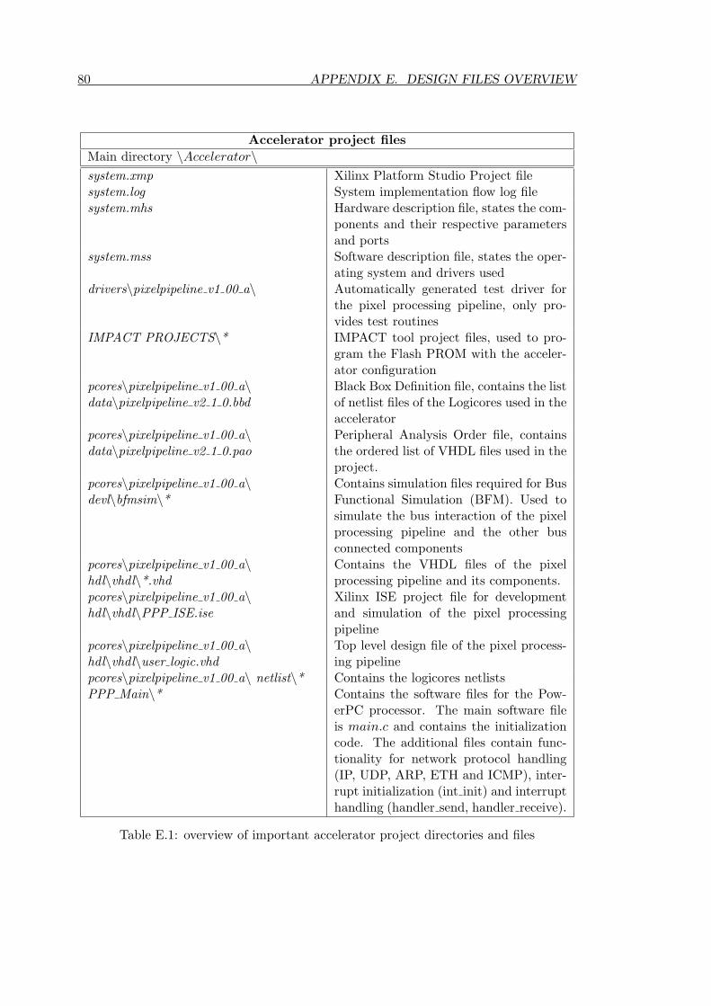
80 APPENDIX E. DESIGN FILES OVERVIEW
Accelerator project filesMain directory \Accelerator\system.xmp Xilinx Platform Studio Project filesystem.log System implementation flow log filesystem.mhs Hardware description file, states the com-
ponents and their respective parametersand ports
system.mss Software description file, states the oper-ating system and drivers used
drivers\pixelpipeline v1 00 a\ Automatically generated test driver forthe pixel processing pipeline, only pro-vides test routines
IMPACT PROJECTS\* IMPACT tool project files, used to pro-gram the Flash PROM with the acceler-ator configuration
pcores\pixelpipeline v1 00 a\data\pixelpipeline v2 1 0.bbd
Black Box Definition file, contains the listof netlist files of the Logicores used in theaccelerator
pcores\pixelpipeline v1 00 a\data\pixelpipeline v2 1 0.pao
Peripheral Analysis Order file, containsthe ordered list of VHDL files used in theproject.
pcores\pixelpipeline v1 00 a\devl\bfmsim\*
Contains simulation files required for BusFunctional Simulation (BFM). Used tosimulate the bus interaction of the pixelprocessing pipeline and the other busconnected components
pcores\pixelpipeline v1 00 a\hdl\vhdl\*.vhd
Contains the VHDL files of the pixelprocessing pipeline and its components.
pcores\pixelpipeline v1 00 a\hdl\vhdl\PPP ISE.ise
Xilinx ISE project file for developmentand simulation of the pixel processingpipeline
pcores\pixelpipeline v1 00 a\hdl\vhdl\user logic.vhd
Top level design file of the pixel process-ing pipeline
pcores\pixelpipeline v1 00 a\ netlist\* Contains the logicores netlistsPPP Main\* Contains the software files for the Pow-
erPC processor. The main software fileis main.c and contains the initializationcode. The additional files contain func-tionality for network protocol handling(IP, UDP, ARP, ETH and ICMP), inter-rupt initialization (int init) and interrupthandling (handler send, handler receive).
Table E.1: overview of important accelerator project directories and files

E.4. DEMONSTRATION SOFTWARE 81
Pipeline components filesMain directory \Components\absdiff\* Absolute difference component; project
file, design files and simulation filesclosing5\* Closing component; project file, design
files and simulation filesconv5\* General 5x5 Convolution component;
project file, design files and simulationfiles
csconv\* Color Space Conversion component;project file, design files and simulationfiles
erodil5\* Erosion/Dilation component; project file,design files and simulation files
localcount\* 7x7 Local Count component; project file,design files and simulation files
padds24\* 24-Bit Signed Adder component; projectfile, design files and simulation files
pdelay1\* 1-Bit Delaying Pipeline Register compo-nent; project file, design files and simula-tion files
pdelay1 16\* 1-Bit Delaying Pipeline Register compo-nent (FIFO depth of 16), design files andsimulation files
pdelay16\* 16-Bit Delaying Pipeline Register compo-nent; project file, design files and simula-tion files
divu19\* 19-Bit Unsigned Divider component;project file, design files and simulationfiles
pmults16\* 16-Bit Signed Multiplier component;project file, design files and simulationfiles
preg32\* 32-Bit Pipeline Register component;project file, design files and simulationfiles
pthreshold32\* 32-Bit Threshold component; project file,design files and simulation files
verification results\* Verification results of the individual com-ponents
Table E.2: overview of important accelerator project directories and files

82 APPENDIX E. DESIGN FILES OVERVIEW
directory \Software\PPPSoftwareDemo, the accelerator demonstration project files canbe found in the directory \Software\demo1.
E.5 Miscellaneous
The CDROM also contains miscellaneous files. The directory \Miscellaneous\TestImagescontains the original source images which have been used to verify the hardware compo-nents. The directory \Miscellaneous\makeECFmodel contains the Matlab program forinitializing the Accelerator parameters. It will generate an output file c : \pppparam.txtwhich contains the parameters for the pixel processing pipeline. These parameters willbe read by the demonstration application demo1 and send to the accelerator upon startof the application.

Curriculum Vitae
Bart de Ruijsscher was born in Oostburg, theNetherlands on April 20, 1981. After receivinghis HAVO diploma in 1999 he started the Electri-cal Engineering study at the Zeeland Universityof Professional Education. He gained industry ex-perience at both Philips Remote Control Systems,Leuven and Siemens VDO Automotive (formerlyknown as Philips Car Systems), Eindhoven be-fore receiving his B.Sc. in Electrical Engineeringin July 2003. Shortly afterwards, he started theMaster of Science in Computer Engineering studyat the Electrical Engineering Department of DelftUniversity of Technology. His research interestsinclude hardware/software co-design and embed-ded systems for multimedia applications.