msdo l21 robustdesign -...
TRANSCRIPT
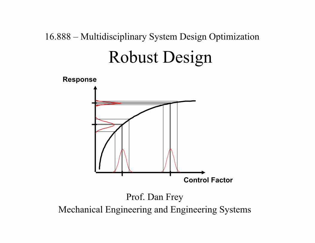
Robust Design
Prof. Dan Frey Mechanical Engineering and Engineering Systems
16.888 – Multidisciplinary System Design Optimization
Control Factor
Response
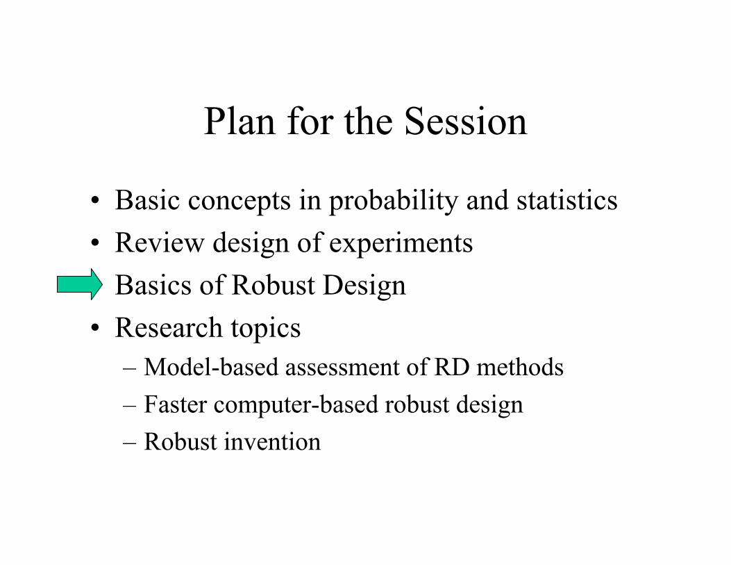
Plan for the Session
• Basic concepts in probability and statistics• Review design of experiments• Basics of Robust Design• Research topics
– Model-based assessment of RD methods – Faster computer-based robust design– Robust invention

Ball and Ramp
Ball
RampFunnel
Response =the time the ball remains in the funnel
Causes of experimental error = ?
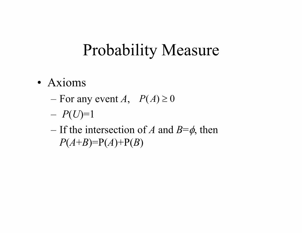
Probability Measure
• Axioms– For any event A,– P(U)=1– If the intersection of A and B= , then
P(A+B)=P(A)+P(B)
0)(AP

Continuous Random Variables
• Can take values anywhere within continuous ranges
• Probability density function
–
–
–
xxfx allfor)(0
1d)( xxfx
xxfbxaPb
ax d)(
x
fx(x)
a b

Histograms
• A graph of continuous data• Approximates a pdf in the limit of large n
0
5
Histogram of Crankpin Diameters
Diameter, Pin #1
Freq
uenc
y
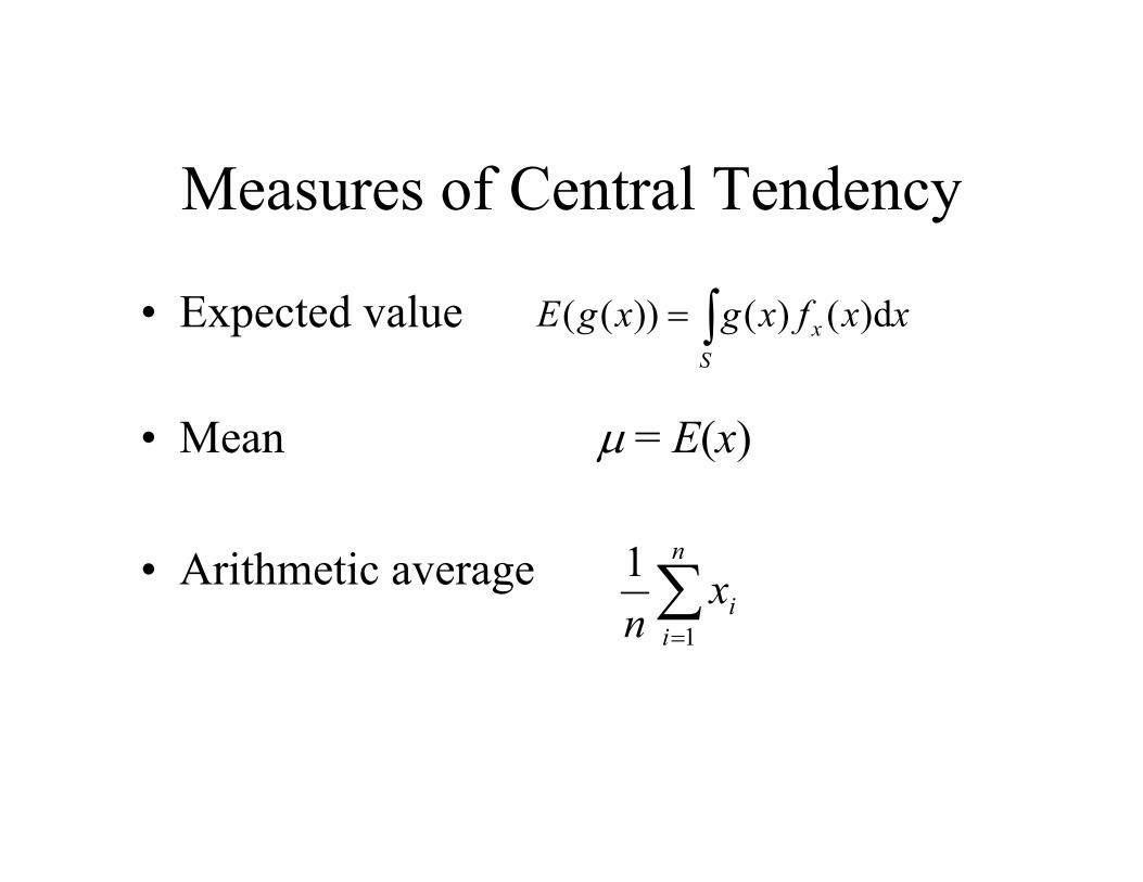
Measures of Central Tendency
• Expected value
• Mean = E(x)
• Arithmetic average
Sx xxfxgxgE d)()())((
n
iix
n 1
1

Measures of Dispersion• Variance
• Standard deviation
• Sample variance
• nth central moment
• nth moment about m
)))((( 2xExE
)))((()( 22 xExExVAR
n
ii xx
nS
1
22 )(1
1
)))((( nxExE
))(( nmxE
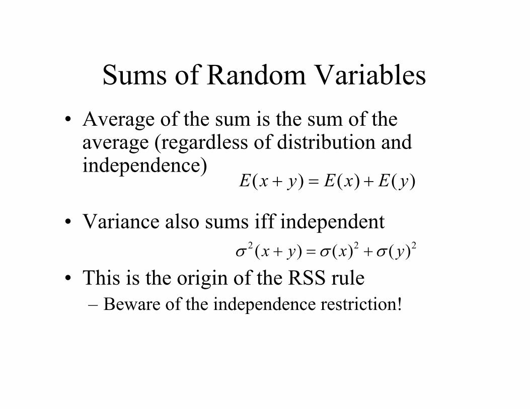
Sums of Random Variables• Average of the sum is the sum of the
average (regardless of distribution and independence)
• Variance also sums iff independent
• This is the origin of the RSS rule– Beware of the independence restriction!
)()()( yExEyxE
222 )()()( yxyx
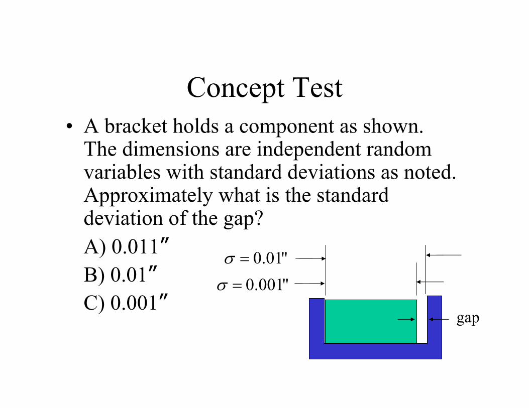
Concept Test• A bracket holds a component as shown.
The dimensions are independent random variables with standard deviations as noted.Approximately what is the standard deviation of the gap?A) 0.011”B) 0.01”C) 0.001”
"001.0"01.0
gap
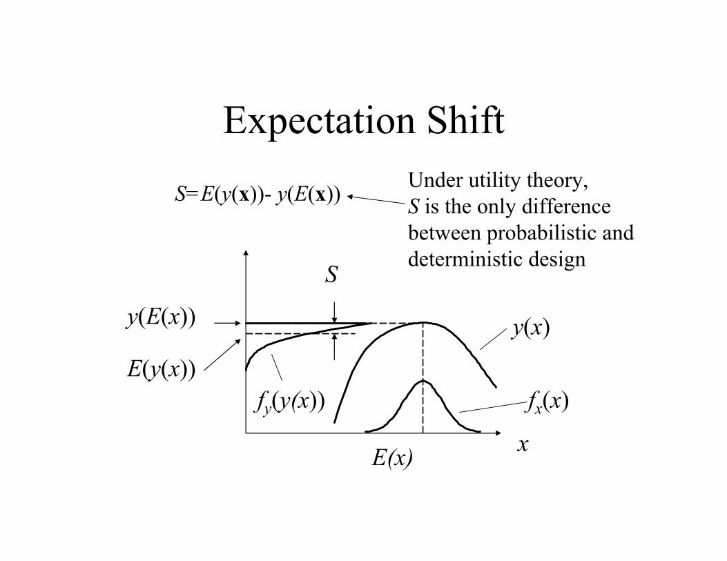
Expectation Shift
x
y(x)
E(x)
y(E(x))
E(y(x))
S
fx(x)fy(y(x))
S=E(y(x))- y(E(x)) Under utility theory,S is the only differencebetween probabilistic and deterministic design
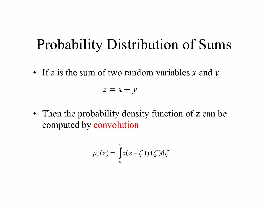
Probability Distribution of Sums
• If z is the sum of two random variables x and y
• Then the probability density function of z can be computed by convolution
yxz
z
z yzxzp d)()()(
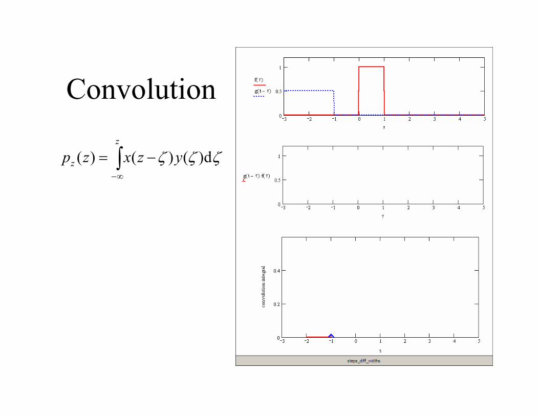
Convolutionz
z yzxzp d)()()(

Convolutionz
z yzxzp d)()()(
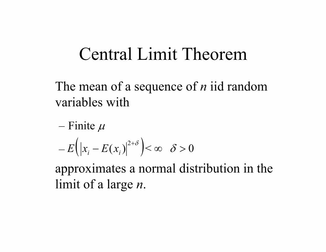
Central Limit Theorem
The mean of a sequence of n iid random variables with
– Finite
–
approximates a normal distribution in the limit of a large n.
0<)( 2ii xExE

Normal Distribution2
2
2)(
21)(
x
x exf
99.7%68.3%
1-2ppb
+6-6 +3+1-1-3
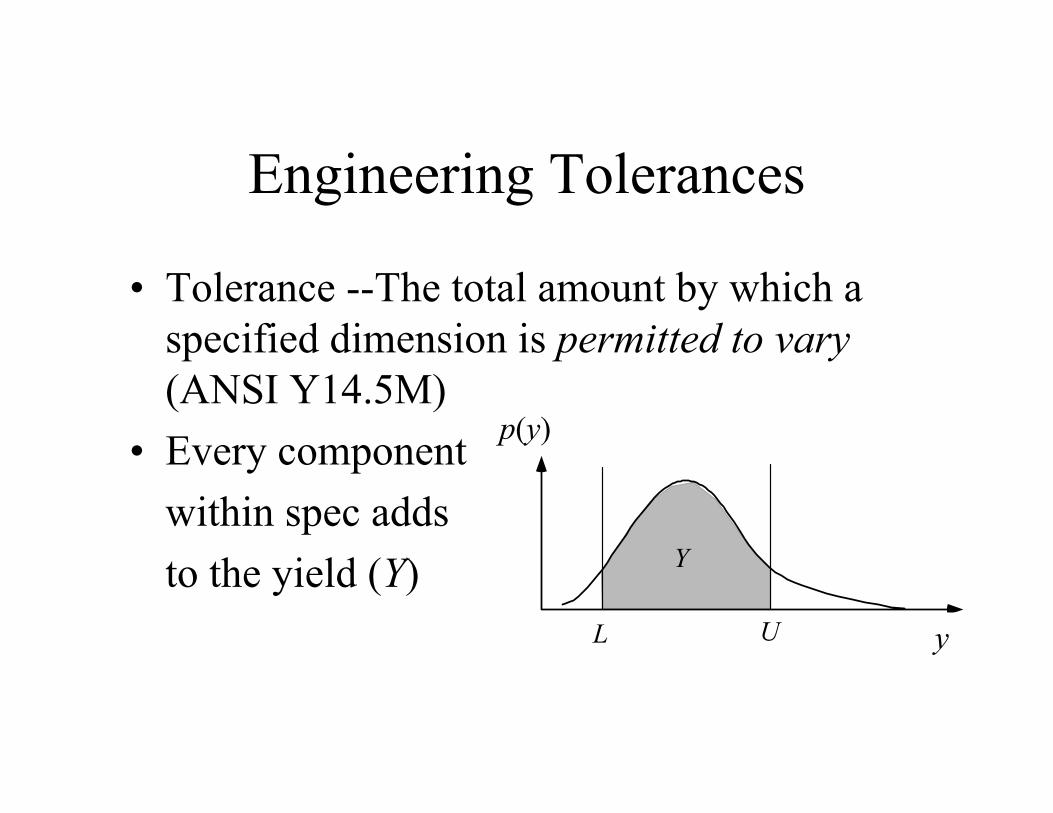
Engineering Tolerances
• Tolerance --The total amount by which a specified dimension is permitted to vary(ANSI Y14.5M)
• Every componentwithin spec addsto the yield (Y)
q
p(q)
L U
Y
y
p(y)

18
Process Capability Indices
• Process Capability Index
• Bias factor
• Performance Index
CU L
p/ 2
3
C C kpk p ( )1
k
U L
U L2
2( ) /
q
p(q)
L UU L2
U L2
Concept Test
• Motorola’s “6 sigma” programs suggest that we should strive for a Cp of 2.0. If this is achieved but the mean is off target so that k=0.5, estimate the process yield.
Plan for the Session
• Basic concepts in probability and statistics• Review design of experiments• Basics of Robust Design• Research topics
– Model-based assessment of RD methods – Faster computer-based robust design– Robust invention
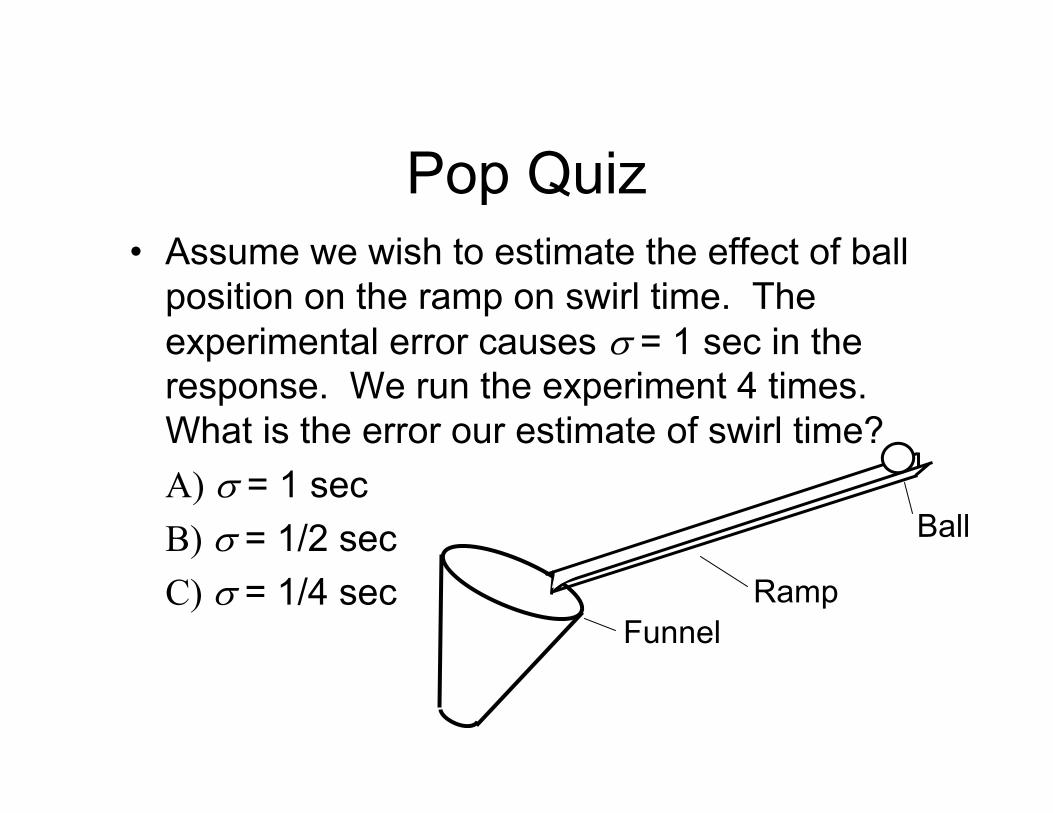
Pop Quiz• Assume we wish to estimate the effect of ball
position on the ramp on swirl time. The experimental error causes = 1 sec in the response. We run the experiment 4 times.What is the error our estimate of swirl time?A) = 1 secB) = 1/2 secC) = 1/4 sec
Ball
RampFunnel
History of DoE
• 1926 – R. A. Fisher introduced the idea of factorial design• 1950-70 – Response surface methods • 1987 – G. Taguchi, System of Experimental Design

Full Factorial Design• This is the 24
• All main effects and interactions can be resolved
• Scales very poorly with number of factors
-1-1-1-1+1-1-1-1-1+1-1-1+1+1-1-1-1-1+1-1+1-1+1-1-1+1+1-1+1+1+1-1-1-1-1+1+1-1-1+1-1+1-1+1+1+1-1+1-1-1+1+1+1-1+1+1-1+1+1+1+1+1+1+1
ResponseDCBA

-1-1-1-1+1-1-1-1-1+1-1-1+1+1-1-1-1-1+1-1+1-1+1-1-1+1+1-1+1+1+1-1-1-1-1+1+1-1-1+1-1+1-1+1+1+1-1+1-1-1+1+1+1-1+1+1-1+1+1+1+1+1+1+1
ResponseDCBA
Replication and Precision
“the same precision as if the whole …
had been devoted to one single component”
– Fisher
The average of trials 1 through 8 has a of 1/8 that of each trial
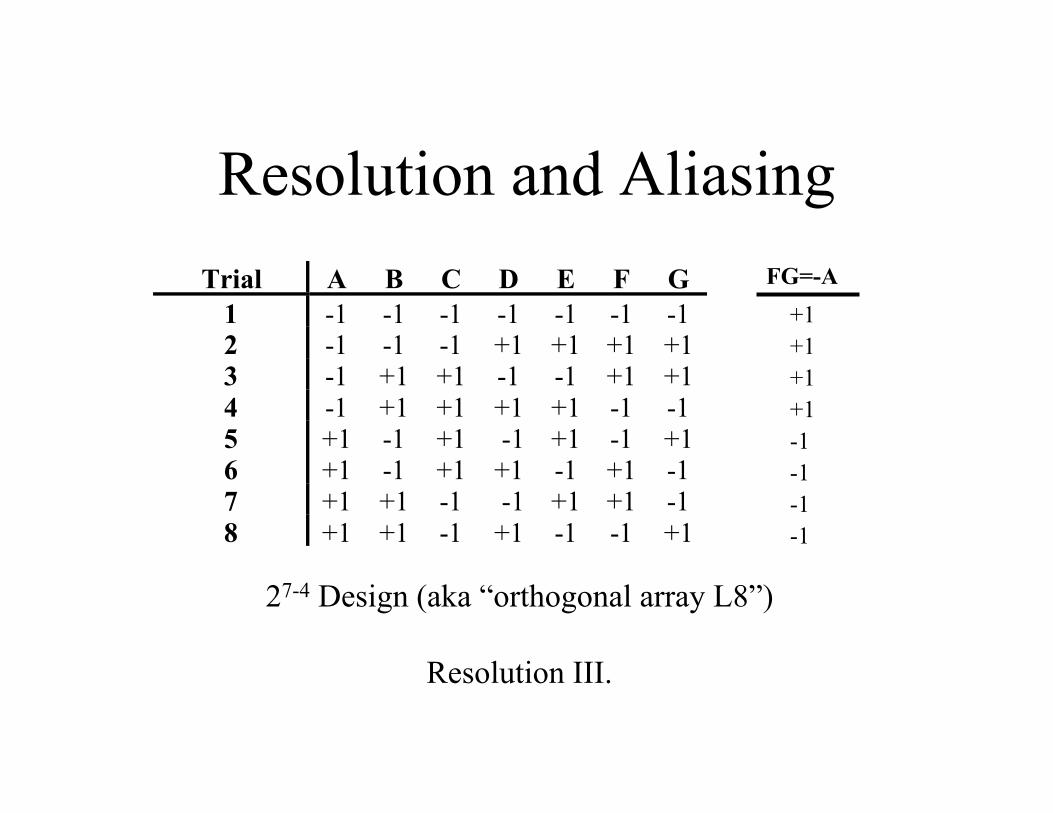
Resolution and AliasingTrial A B C D E F G
1 -1 -1 -1 -1 -1 -1 -12 -1 -1 -1 +1 +1 +1 +13 -1 +1 +1 -1 -1 +1 +14 -1 +1 +1 +1 +1 -1 -15 +1 -1 +1 -1 +1 -1 +16 +1 -1 +1 +1 -1 +1 -17 +1 +1 -1 -1 +1 +1 -18 +1 +1 -1 +1 -1 -1 +1
27-4 Design (aka “orthogonal array L8”)
Resolution III.
FG=-A+1+1+1+1-1-1-1-1
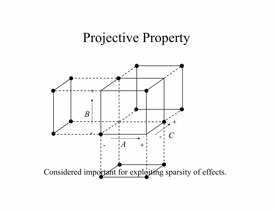
Projective Property
A
B
C
+
-
+
+
--
Considered important for exploiting sparsity of effects.
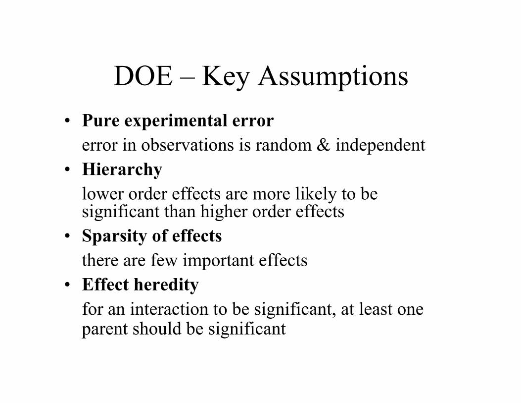
DOE – Key Assumptions• Pure experimental error
error in observations is random & independent • Hierarchy
lower order effects are more likely to be significant than higher order effects
• Sparsity of effectsthere are few important effects
• Effect heredityfor an interaction to be significant, at least one parent should be significant
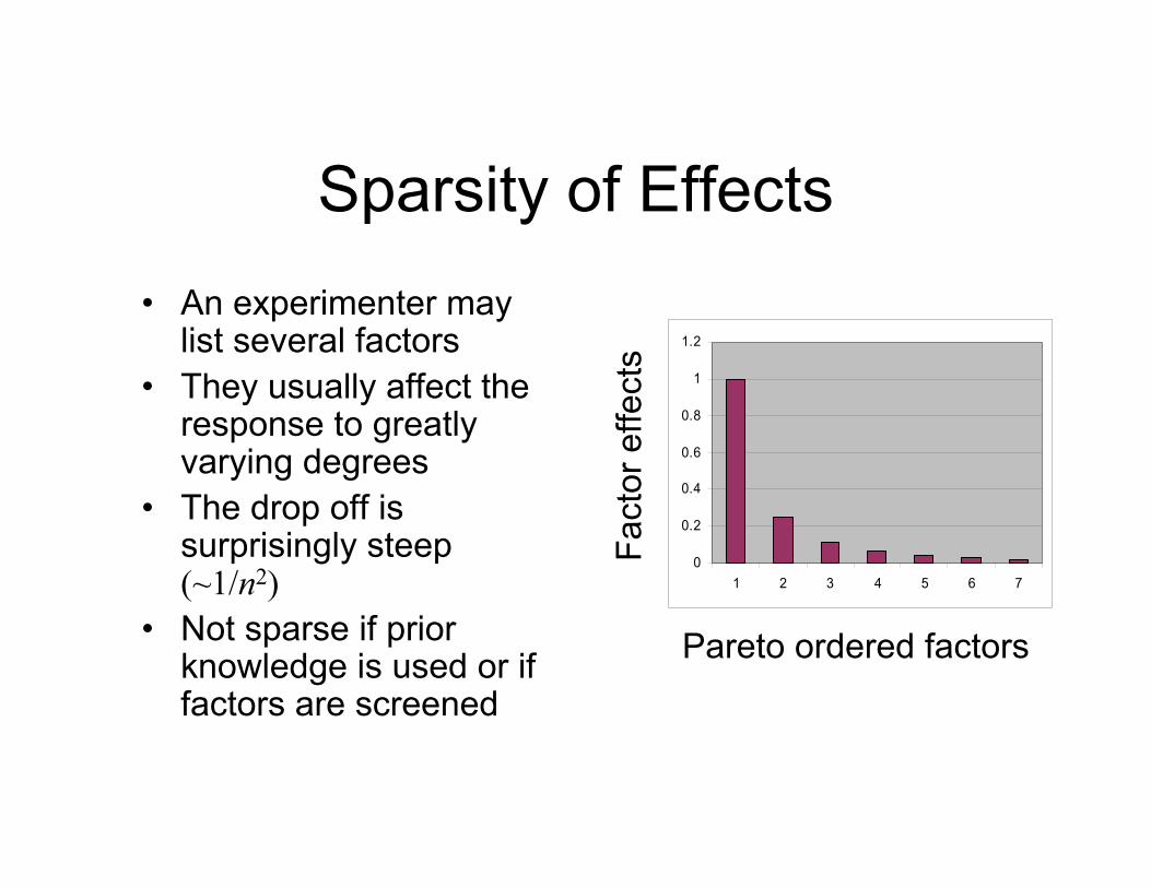
Sparsity of Effects• An experimenter may
list several factors• They usually affect the
response to greatly varying degrees
• The drop off is surprisingly steep (~1/n2)
• Not sparse if prior knowledge is used or if factors are screened
0
0.2
0.4
0.6
0.8
1
1.2
1 2 3 4 5 6 7
Pareto ordered factorsFa
ctor
effe
cts

Hierarchy• Main effects are usually
more important than two-factor interactions
• Two-way interactions are usually more important than three-factor interactions
• And so on• Taylor’s series seems to
support the idea
A B C
AB AC BC
D
AD BD CD
ABC ABD BCDACD
ABCD!
)()()(
0 nafax
n
n
n

Inheritance
• Two-factor interactions are most likely when both participating factors (parents?) are strong
• Two-way interactions are least likely when neither parent is strong
• And so on
A B C
AB AC BC
D
AD BD CD
ABC ABD BCDACD
ABCD
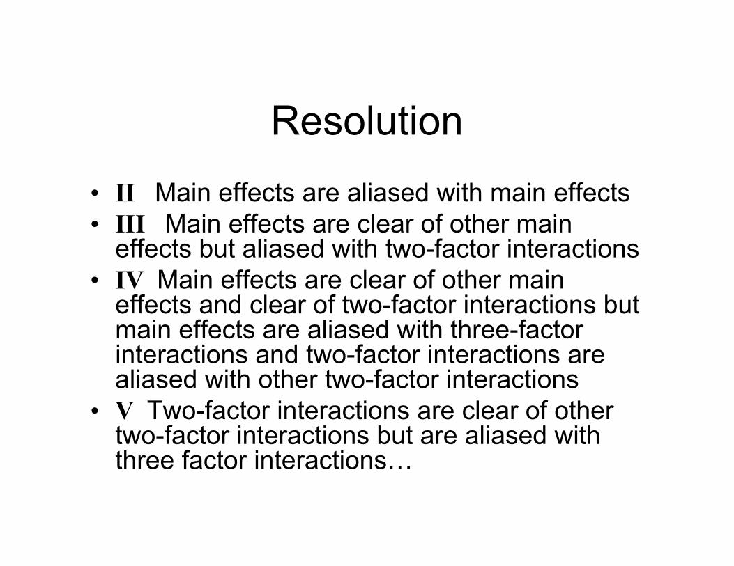
Resolution• II Main effects are aliased with main effects• III Main effects are clear of other main
effects but aliased with two-factor interactions• IV Main effects are clear of other main
effects and clear of two-factor interactions but main effects are aliased with three-factor interactions and two-factor interactions are aliased with other two-factor interactions
• V Two-factor interactions are clear of other two-factor interactions but are aliased with three factor interactions…
Discussion Point
• What are the four most important factors affecting swirl time?
• If you want to have sparsity of effects and hierarchy, how would you formulate the variables?

Important Concepts in DOE• Resolution – the ability of an experiment to
provide estimates of effects that are clear of other effects
• Sparsity of Effects – factor effects are few• Hierarchy – interactions are generally less
significant than main effects• Inheritance – if an interaction is significant, at
least one of its “parents” is usually significant• Efficiency – ability of an experiment to
estimate effects with small error variance
Plan for the Session
• Basic concepts in probability and statistics• Review design of experiments• Basics of Robust Design• Research topics
– Model-based assessment of RD methods – Faster computer-based robust design– Robust invention

Major Concepts of Taguchi Method
• Variation causes quality loss• Two-step optimization• Parameter design via orthogonal arrays• Inducing noise (outer arrays)• Interactions and confirmation
y
L(y)
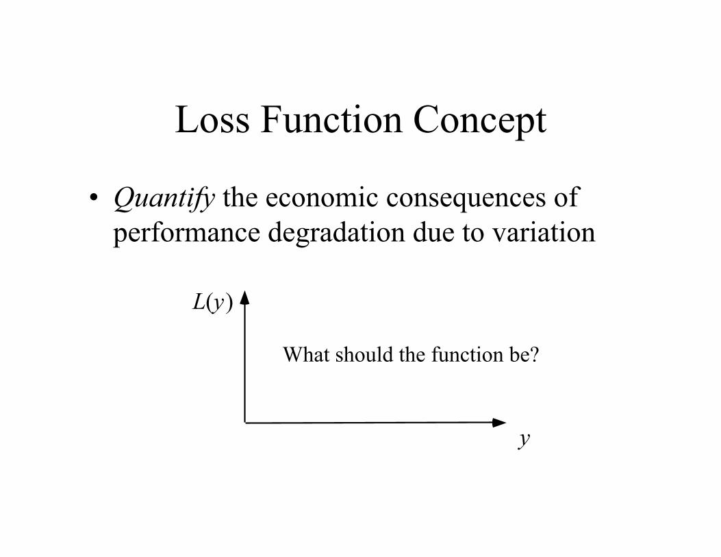
Loss Function Concept
• Quantify the economic consequences of performance degradation due to variation
What should the function be?
y
L(y)
Ao
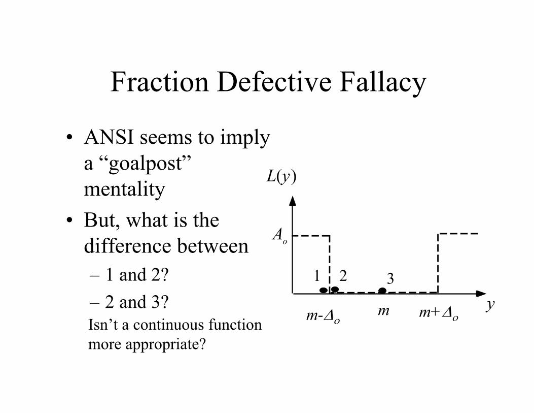
Fraction Defective Fallacy
• ANSI seems to imply a “goalpost” mentality
• But, what is the difference between – 1 and 2?– 2 and 3?
321
Isn’t a continuous function more appropriate?
m m+m-
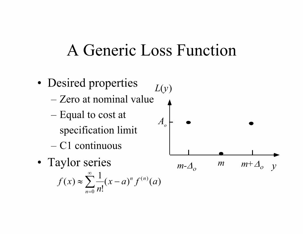
A Generic Loss Function
• Desired properties– Zero at nominal value– Equal to cost at
specification limit– C1 continuous
• Taylor series y
L(y)
Ao
)()(!
1)( )(
0
afaxn
xf nn
n
m m+m-
y
L(y)
quadratic quality loss function
"goal post" loss function
Ao
m m+m-
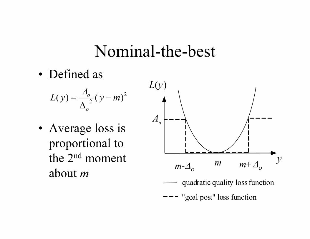
Nominal-the-best• Defined as
• Average loss is proportional to the 2nd momentabout m
22 )()( myAyL
o
o
y
L(y)
quadratic quality loss function
Ao
m m+m-
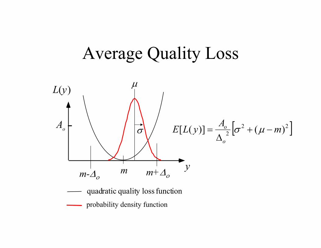
Average Quality Loss
222 )()]([ mAyLE
o
o
probability density function
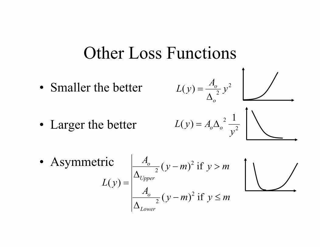
Other Loss Functions
• Smaller the better
• Larger the better
• Asymmetric
22)( yAyL
o
o
22 1)(
yAyL oo
mymyA
mymyA
yL
Lower
o
Upper
o
if)(
if)()(
22
22
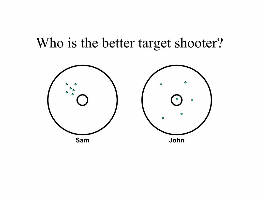
Who is the better target shooter?
Sam John
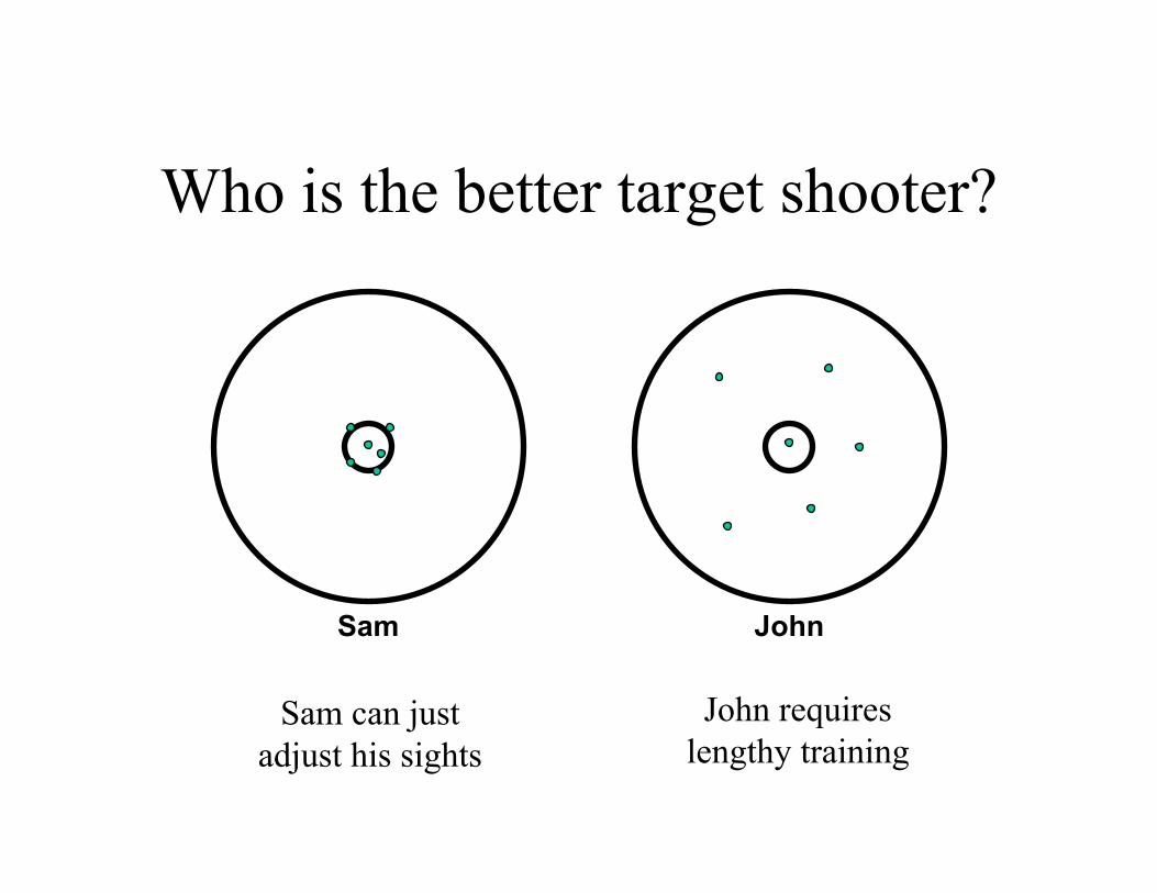
Who is the better target shooter?
Sam John
Sam can just adjust his sights
John requires lengthy training
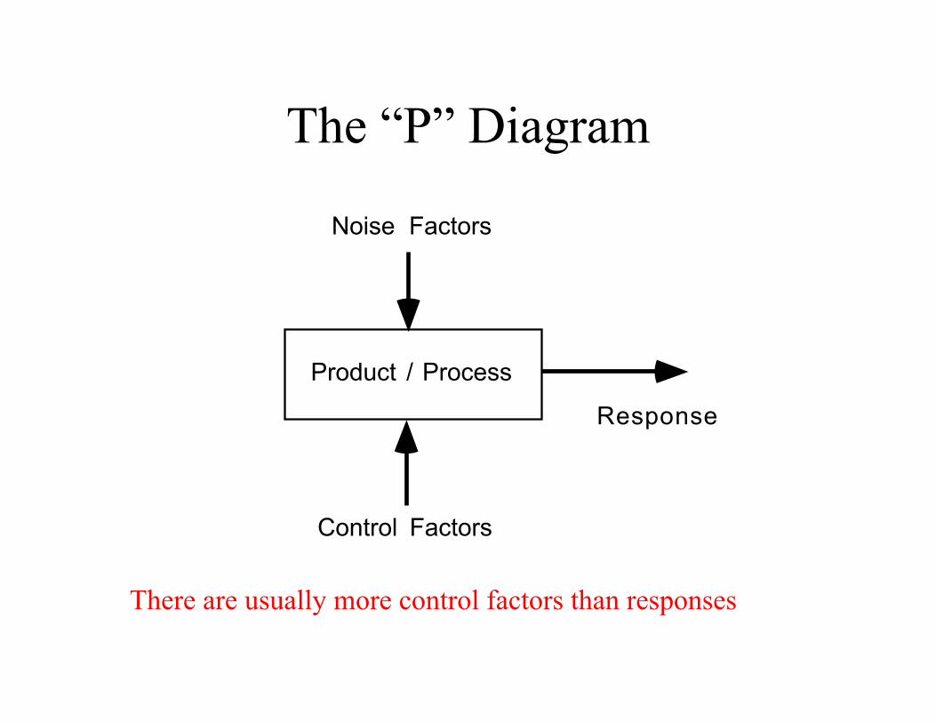
The “P” Diagram
Product / Process
Response
Noise Factors
Control Factors
There are usually more control factors than responses
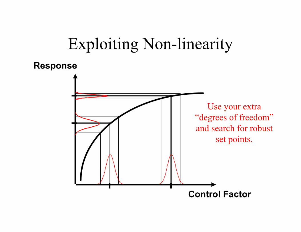
Exploiting Non-linearity
Control Factor
Response
Use your extra “degrees of freedom” and search for robust
set points.
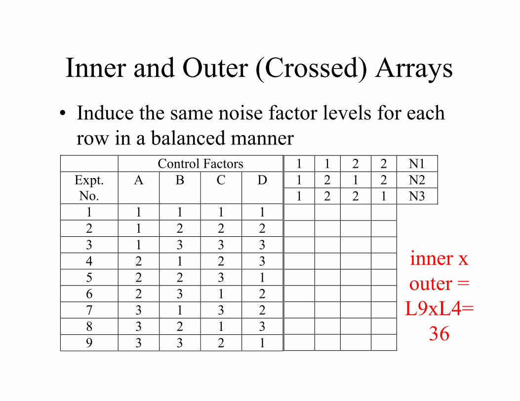
Inner and Outer (Crossed) Arrays • Induce the same noise factor levels for each
row in a balanced manner Control Factors
Expt.No.
A B C D
1 1 1 1 12 1 2 2 23 1 3 3 34 2 1 2 35 2 2 3 16 2 3 1 27 3 1 3 28 3 2 1 39 3 3 2 1
1 1 2 2 N11 2 1 2 N21 2 2 1 N3
inner xouter =L9xL4=
36
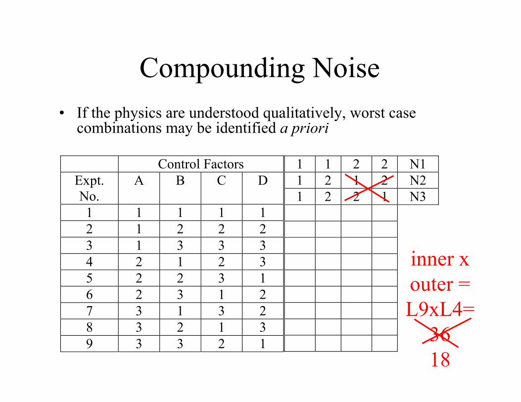
Compounding Noise • If the physics are understood qualitatively, worst case
combinations may be identified a priori
Control FactorsExpt.No.
A B C D
1 1 1 1 12 1 2 2 23 1 3 3 34 2 1 2 35 2 2 3 16 2 3 1 27 3 1 3 28 3 2 1 39 3 3 2 1
1 1 2 2 N11 2 1 2 N21 2 2 1 N3
inner xouter =L9xL4=
3618
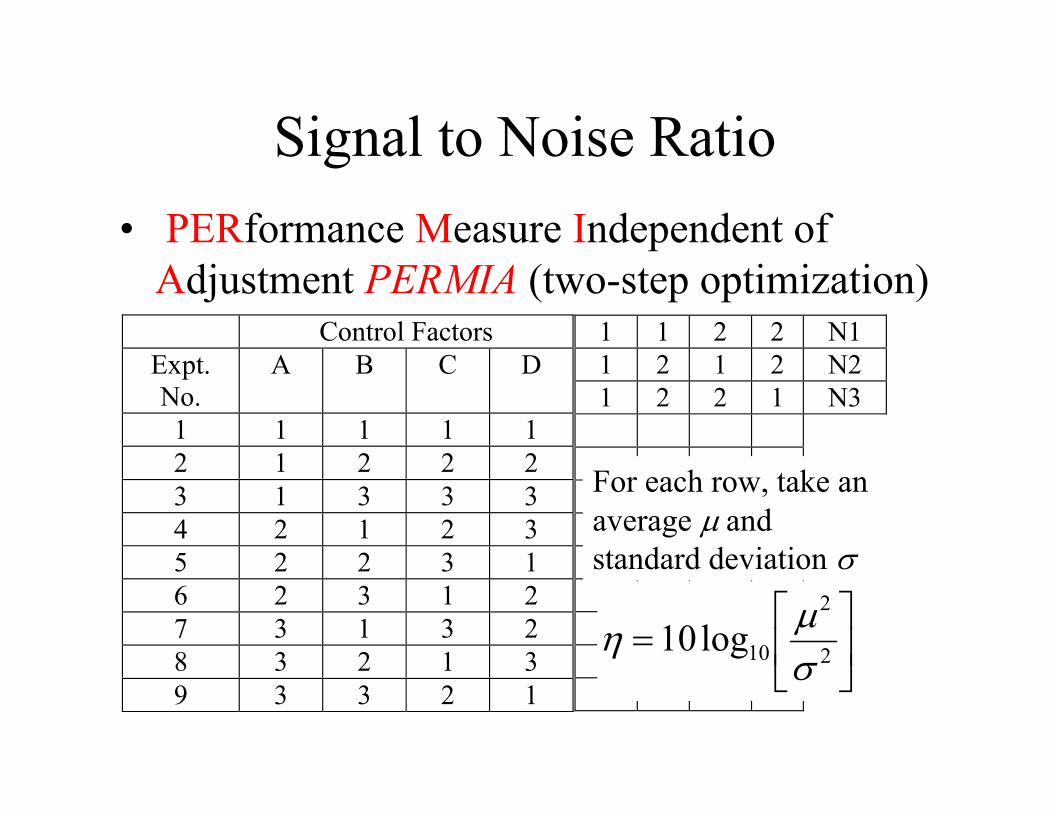
Signal to Noise Ratio• PERformance Measure Independent of
Adjustment PERMIA (two-step optimization) Control Factors
Expt.No.
A B C D
1 1 1 1 12 1 2 2 23 1 3 3 34 2 1 2 35 2 2 3 16 2 3 1 27 3 1 3 28 3 2 1 39 3 3 2 1
1 1 2 2 N11 2 1 2 N21 2 2 1 N3
2
2
10log10
For each row, take an average andstandard deviation
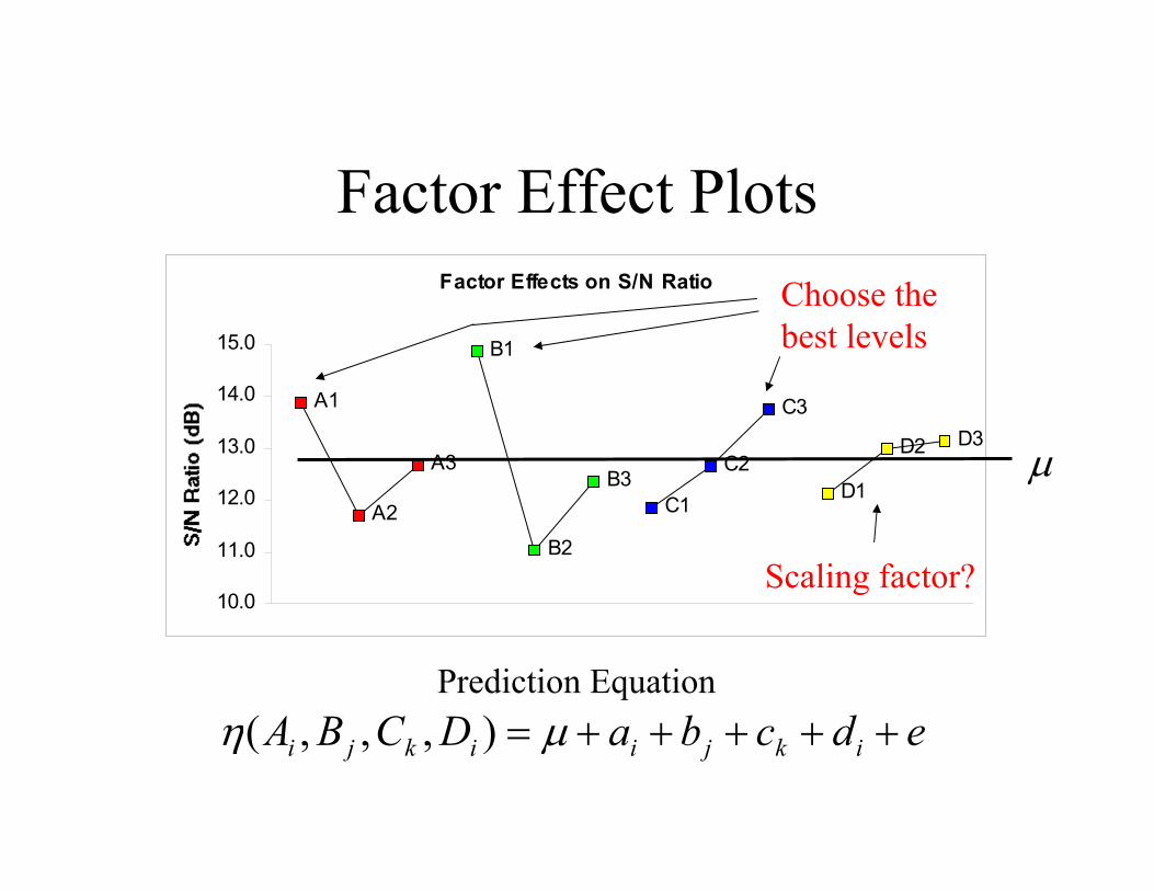
Factor Effects on S/N Ratio
A1
A2
A3
B1
B2
B3C1
C2
C3
D1
D2 D3
10.0
11.0
12.0
13.0
14.0
15.0
Factor Effect Plots
edcbaDCBA ikjiikji ),,,(Prediction Equation
Choose the best levels
Scaling factor?
Factor Effects on S/N Ratio
A1
A2
A3
B1
B2
B3C1
C2
C3
D1
D2 D3
10.0
11.0
12.0
13.0
14.0
15.0
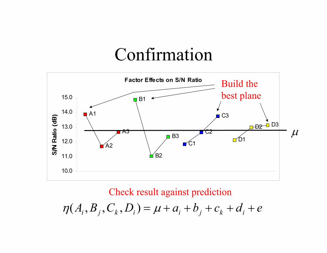
Confirmation
edcbaDCBA ikjiikji ),,,(
Build the best plane
Check result against prediction
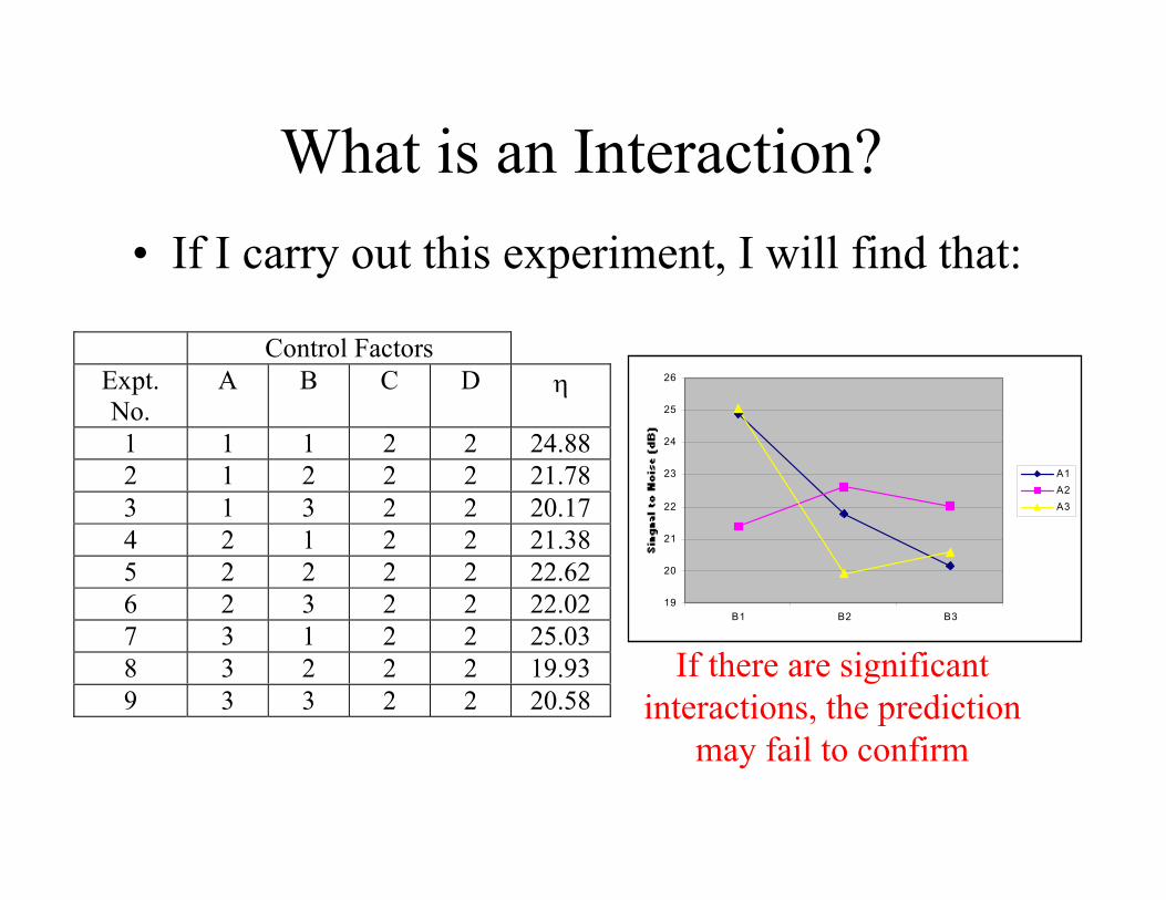
What is an Interaction?• If I carry out this experiment, I will find that:
19
20
21
22
23
24
25
26
B1 B2 B3
A1A2A3
If there are significant interactions, the prediction
may fail to confirm
Control FactorsExpt.No.
A B C D
1 1 1 2 2 24.882 1 2 2 2 21.783 1 3 2 2 20.174 2 1 2 2 21.385 2 2 2 2 22.626 2 3 2 2 22.027 3 1 2 2 25.038 3 2 2 2 19.939 3 3 2 2 20.58
Major Concepts of Taguchi Method
• Variation causes quality loss• Two-step optimization• Parameter design via orthogonal arrays• Inducing noise (outer arrays)• Interactions and confirmation
Some Concerns with Taguchi Methods
• Interactions can often cause failure to confirm
• Two step optimization not really needed• Use of S/N often not a useful as modeling
the response explicitly• Some experts consider crossed arrays are
less efficient than putting noise in the inner array

References• Byrne, Diane M. and Taguchi, Shin
“The Taguchi Approach to Parameter Design”Quality Progress, Dec 1987.
• Phadke, Madhav S., 1989, QualityEngineering Using Robust DesignPrentice Hall, Englewood Cliffs, 1989.
• Logothetis and Wynn, Quality Through Design, Oxford Series on Advanced Manufacturing, 1994.
• Wu and Hamada, 2000, Experiments:Planning, Analysis and Parameter Design Optimization, Wiley & Sons, Inc., NY.
Plan for the Session
• Basic concepts in probability and statistics• Review design of experiments• Basics of Robust Design• Research topics
– Model-based assessment of RD methods – Faster computer-based robust design– Robust invention
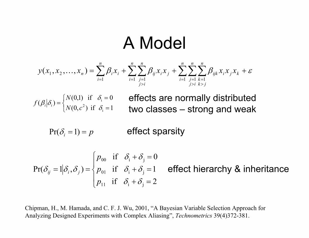
A Model
1if),0(0if)1,0(
)(i
2i
cNN
f ii
pi )1Pr(
effects are normally distributedtwo classes – strong and weak
effect sparsity
Chipman, H., M. Hamada, and C. F. J. Wu, 2001, “A Bayesian Variable Selection Approach for Analyzing Designed Experiments with Complex Aliasing”, Technometrics 39(4)372-381.
2if1if0if
),1Pr(
ji11
ji01
ji00
ppp
jiij effect hierarchy & inheritance
kji
n
i
n
ijj
n
jkk
ijkji
n
i
n
ijj
ij
n
iiin xxxxxxxxxy
1 1 11 1121 ),,,(
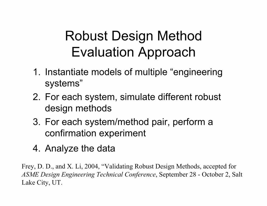
Robust Design MethodEvaluation Approach
1. Instantiate models of multiple “engineering systems”
2. For each system, simulate different robust design methods
3. For each system/method pair, perform a confirmation experiment
4. Analyze the data
Frey, D. D., and X. Li, 2004, “Validating Robust Design Methods, accepted for ASME Design Engineering Technical Conference, September 28 - October 2, Salt Lake City, UT.

Including Noise Factors in the Model
1),0(~ 1 miwNIDxi
11,1 nmixi
),0(~ 22wNID
kji
n
i
n
ijj
n
jkk
ijkji
n
i
n
ijj
ij
n
iiin xxxxxxxxxy
1 1 11 1121 ),,,(
The first m are noise factors
The rest are control factors with two levels
Observations of the response y are subject to
experimental error
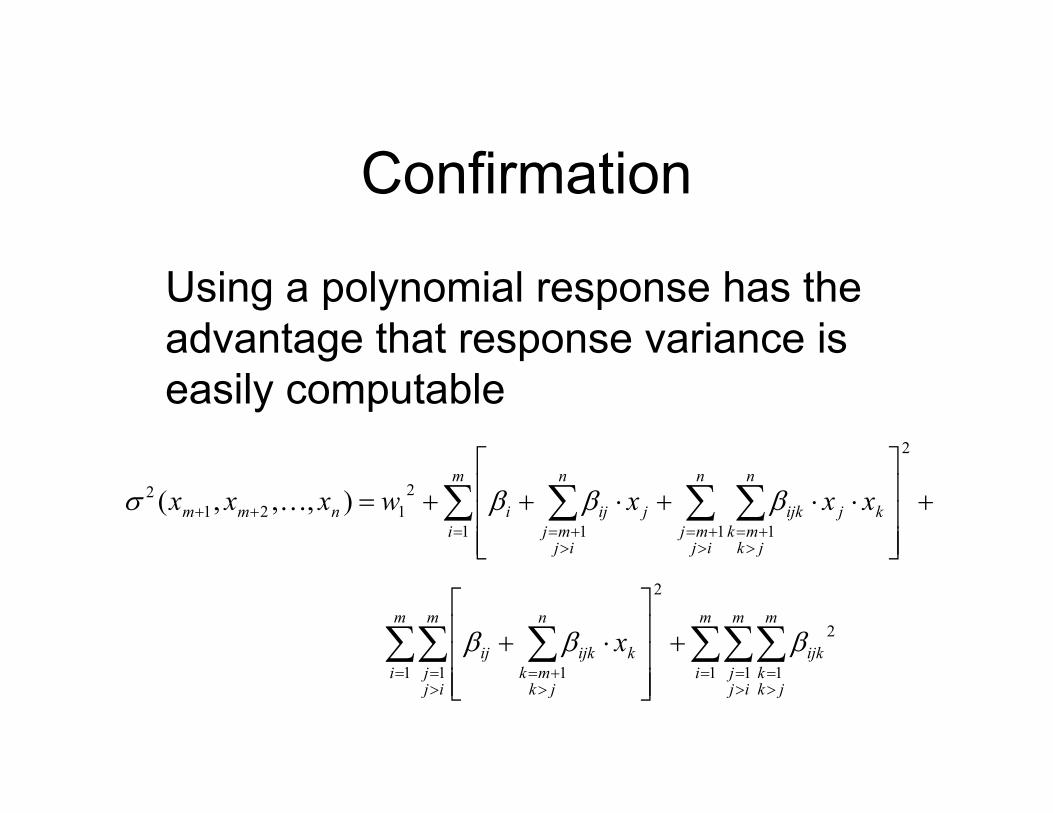
Confirmation
Using a polynomial response has the advantage that response variance is easily computable
m
i
m
ijj
m
jkk
ijk
m
i
m
ijj
n
jkmk
kijkij
m
i
n
ijmj
n
jkmk
kjijk
n
ijmj
jijinmm
x
xxxwxxx
1 1 1
2
1 1
2
1
2
1 1 11
2121
2 ),,,(
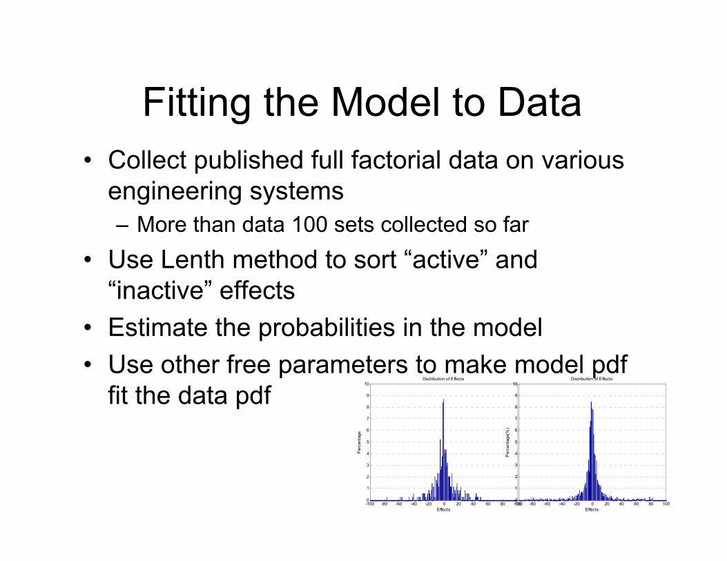
Fitting the Model to Data• Collect published full factorial data on various
engineering systems – More than data 100 sets collected so far
• Use Lenth method to sort “active” and “inactive” effects
• Estimate the probabilities in the model• Use other free parameters to make model pdf
fit the data pdf
-100 -80 -60 -40 -20 0 20 40 60 80 1000
1
2
3
4
5
6
7
8
9
10
Effects
Per
cent
age
Distribution of Effects
-100 -80 -60 -40 -20 0 20 40 60 80 1000
1
2
3
4
5
6
7
8
9
10
EffectsP
erce
ntag
e(%
)
Distribution of Effects

Different Variants of the Model
p p11 p01 p00 p111 p011 p001 p000
Basic WH 0.25 0.25 0.1 0 0.25 0.1 0 0 Basic low w 0.25 0.25 0.1 0 0.25 0.1 0 0
Basic 2nd order 0.25 0.25 0.1 0 N/A N/A N/A N/AFitted WH 0.43 0.31 0.04 0 0.17 0.08 0.02 0
Fitted low w 0.43 0.31 0.04 0 0.17 0.08 0.02 0 Fitted 2nd order 0.43 0.31 0.04 0 N/A N/A N/A N/A
c s1 s2 w1 w2
Basic WH 10 1 1 1 1 Basic low w 10 1 1 0.1 0.1
Basic 2nd order 10 1 0 1 1 Fitted WH 15 1/3 2/3 1 1
Fitted low w 15 1/3 2/3 0.1 0.1 Fitted 2nd order 15 1/3 0 1 1
The model that drives much of DOE
& Robust Design
The model I think is most realistic
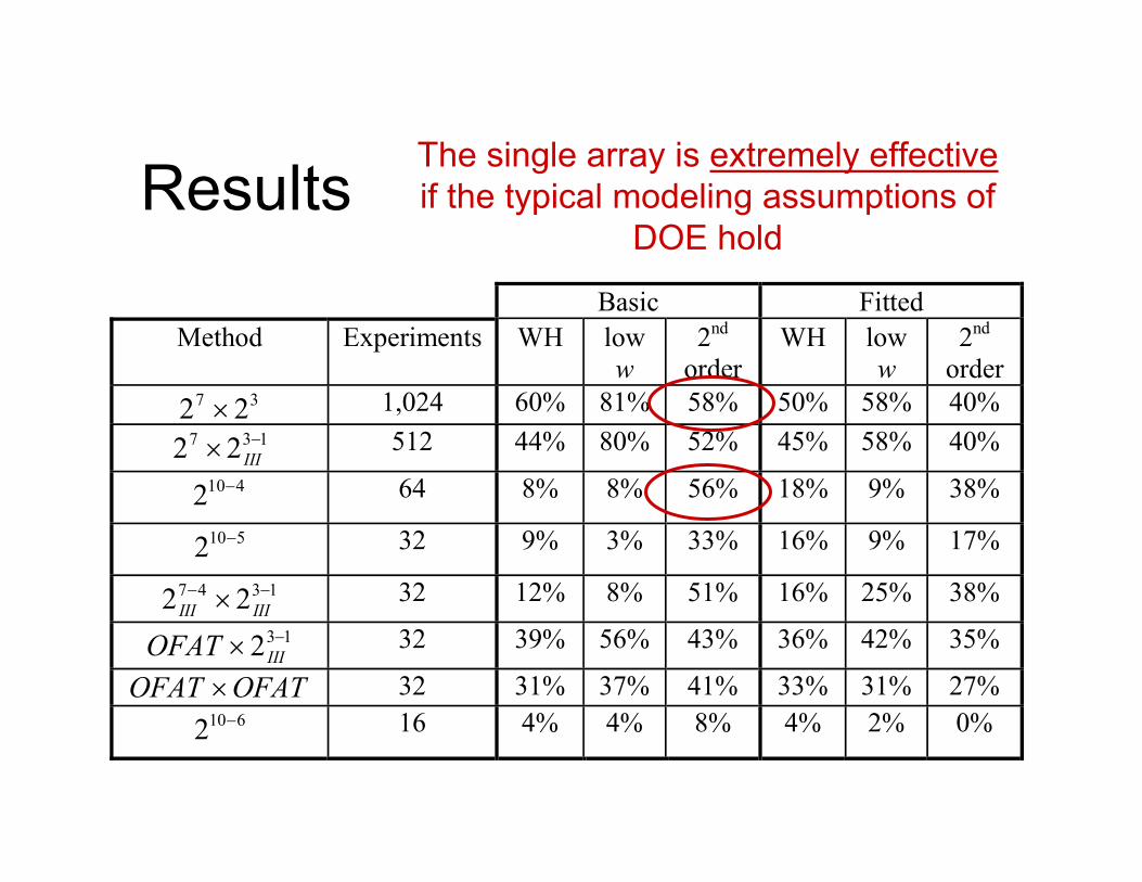
Results Basic Fitted
Method Experiments WH low w
2nd
order WH low
w2nd
order 37 22 1,024 60% 81% 58% 50% 58% 40%
137 22 III512 44% 80% 52% 45% 58% 40%
4102 64 8% 8% 56% 18% 9% 38%
5102 32 9% 3% 33% 16% 9% 17%
1347 22 IIIIII32 12% 8% 51% 16% 25% 38%
132 IIIOFAT 32 39% 56% 43% 36% 42% 35%
OFATOFAT 32 31% 37% 41% 33% 31% 27% 6102 16 4% 4% 8% 4% 2% 0%
The single array is extremely effectiveif the typical modeling assumptions of
DOE hold
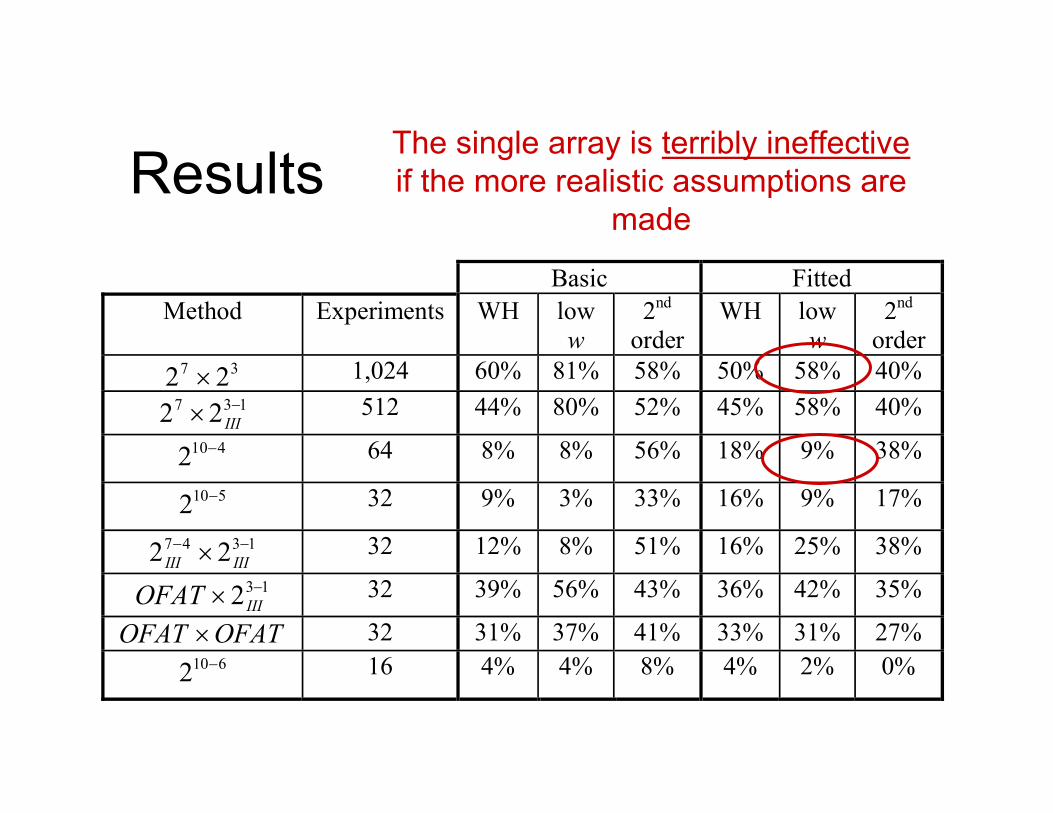
Results Basic Fitted
Method Experiments WH low w
2nd
order WH low
w2nd
order 37 22 1,024 60% 81% 58% 50% 58% 40%
137 22 III512 44% 80% 52% 45% 58% 40%
4102 64 8% 8% 56% 18% 9% 38%
5102 32 9% 3% 33% 16% 9% 17%
1347 22 IIIIII32 12% 8% 51% 16% 25% 38%
132 IIIOFAT 32 39% 56% 43% 36% 42% 35%
OFATOFAT 32 31% 37% 41% 33% 31% 27% 6102 16 4% 4% 8% 4% 2% 0%
The single array is terribly ineffective if the more realistic assumptions are
made

Results Basic Fitted
Method Experiments WH low w
2nd
order WH low
w2nd
order 37 22 1,024 60% 81% 58% 50% 58% 40%
137 22 III512 44% 80% 52% 45% 58% 40%
4102 64 8% 8% 56% 18% 9% 38%
5102 32 9% 3% 33% 16% 9% 17%
1347 22 IIIIII32 12% 8% 51% 16% 25% 38%
132 IIIOFAT 32 39% 56% 43% 36% 42% 35%
OFATOFAT 32 31% 37% 41% 33% 31% 27% 6102 16 4% 4% 8% 4% 2% 0%
Taguchi’s crossed arrays are more effective than single arrays
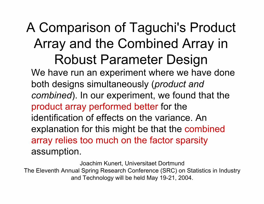
A Comparison of Taguchi's Product Array and the Combined Array in
Robust Parameter DesignWe have run an experiment where we have done both designs simultaneously (product and combined). In our experiment, we found that the product array performed better for the identification of effects on the variance. An explanation for this might be that the combinedarray relies too much on the factor sparsityassumption.
Joachim Kunert, Universitaet DortmundThe Eleventh Annual Spring Research Conference (SRC) on Statistics in Industry
and Technology will be held May 19-21, 2004.
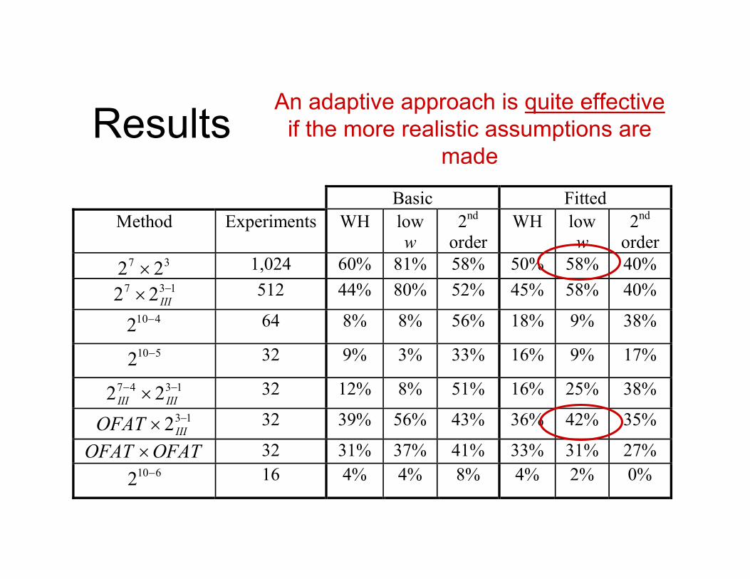
Results Basic Fitted
Method Experiments WH low w
2nd
order WH low
w2nd
order 37 22 1,024 60% 81% 58% 50% 58% 40%
137 22 III512 44% 80% 52% 45% 58% 40%
4102 64 8% 8% 56% 18% 9% 38%
5102 32 9% 3% 33% 16% 9% 17%
1347 22 IIIIII32 12% 8% 51% 16% 25% 38%
132 IIIOFAT 32 39% 56% 43% 36% 42% 35%
OFATOFAT 32 31% 37% 41% 33% 31% 27% 6102 16 4% 4% 8% 4% 2% 0%
An adaptive approach is quite effective if the more realistic assumptions are
made
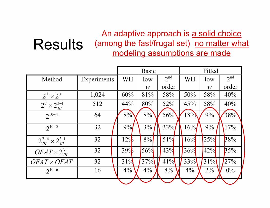
Results Basic Fitted
Method Experiments WH low w
2nd
order WH low
w2nd
order 37 22 1,024 60% 81% 58% 50% 58% 40%
137 22 III512 44% 80% 52% 45% 58% 40%
4102 64 8% 8% 56% 18% 9% 38%
5102 32 9% 3% 33% 16% 9% 17%
1347 22 IIIIII32 12% 8% 51% 16% 25% 38%
132 IIIOFAT 32 39% 56% 43% 36% 42% 35%
OFATOFAT 32 31% 37% 41% 33% 31% 27% 6102 16 4% 4% 8% 4% 2% 0%
An adaptive approach is a solid choice(among the fast/frugal set) no matter what
modeling assumptions are made
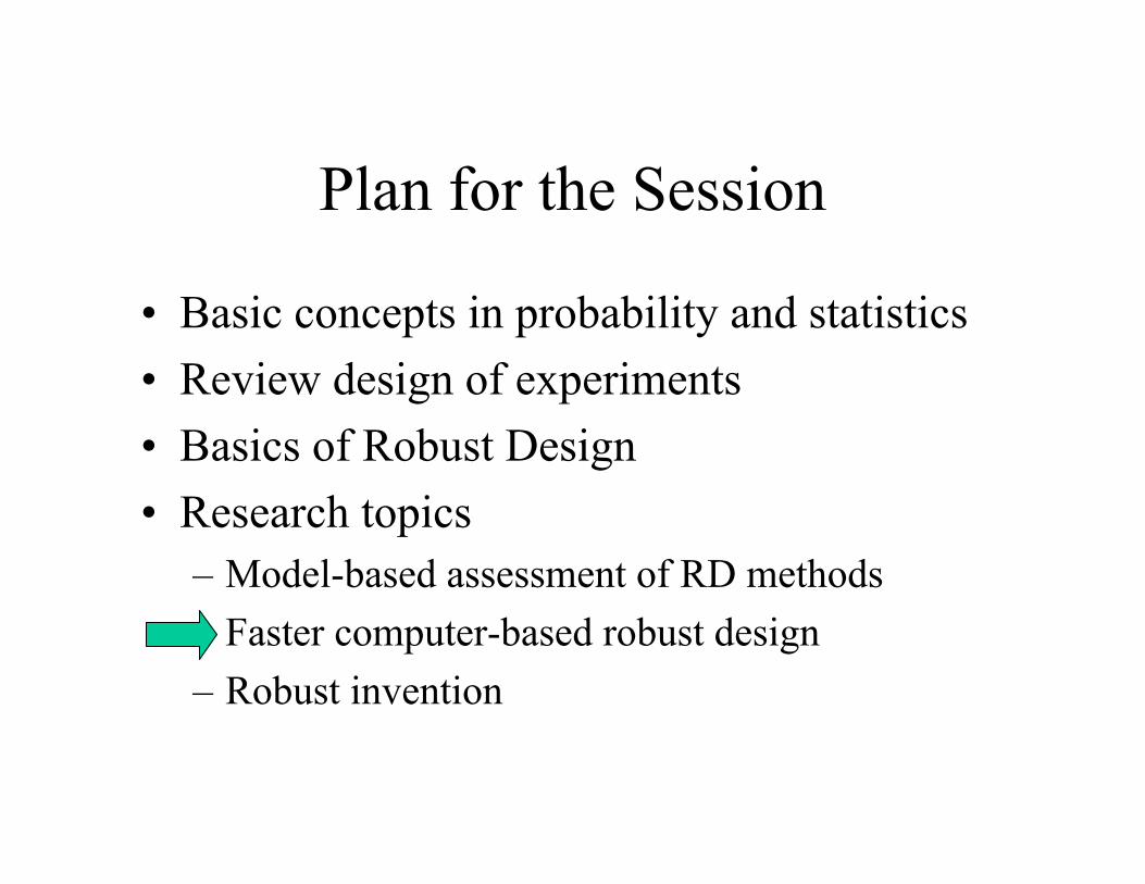
Plan for the Session
• Basic concepts in probability and statistics• Review design of experiments• Basics of Robust Design• Research topics
– Model-based assessment of RD methods – Faster computer-based robust design– Robust invention
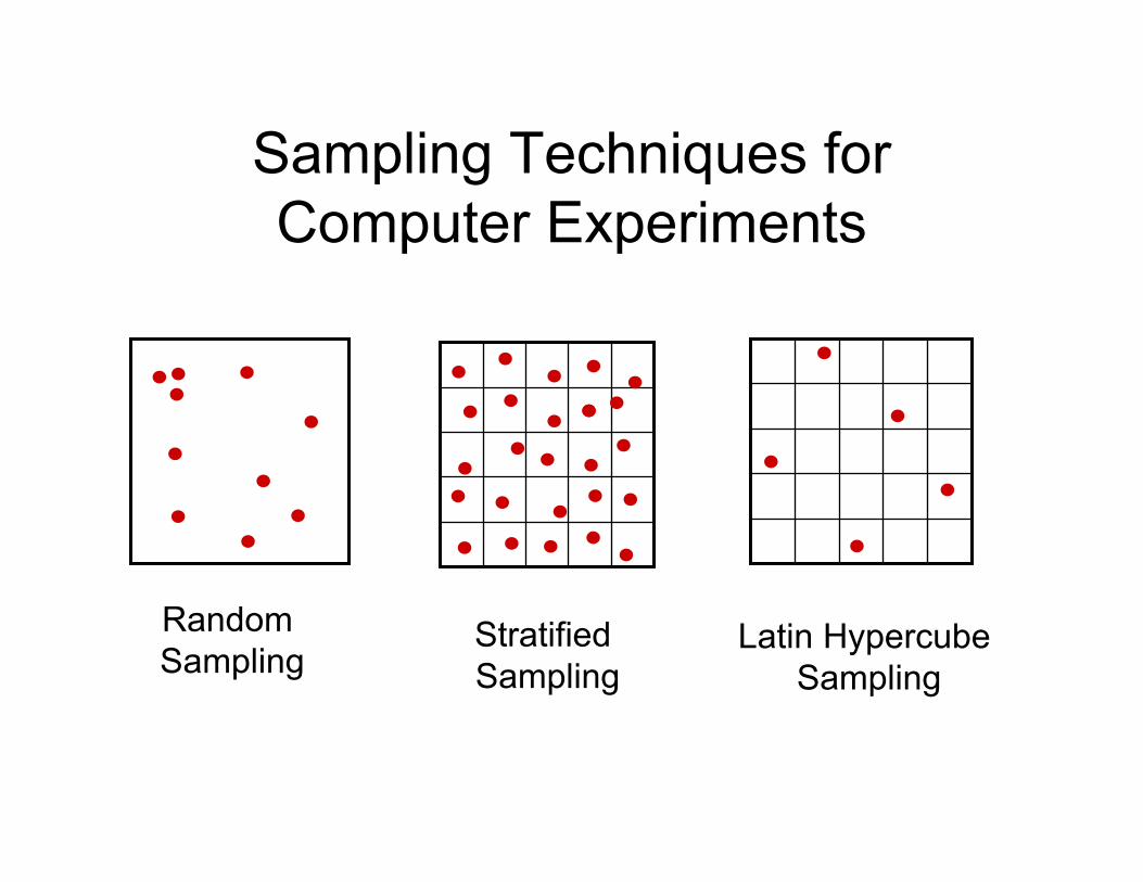
Sampling Techniques for Computer Experiments
RandomSampling
StratifiedSampling
Latin Hypercube Sampling
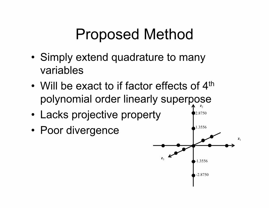
Proposed Method• Simply extend quadrature to many
variables• Will be exact to if factor effects of 4th
polynomial order linearly superpose• Lacks projective property• Poor divergence
z1
z2
z3
1.3556
2.8750
-1.3556
-2.8750

Why Neglect Interactions?
n
i
n
jij
n
kjk
n
lkl ijkkijllikklijjljkkliijlijllijkkikllijjk
jklliijkjjkkiilljjlliikkkklliijjijkl
n
i
n
jij
n
kjk
iijkjkkkiijkjjjkijkkijjjijjkiiik
ijkkiiijjjkkiikkiikkiijjjjkkiijjikkijj
jjkiikjkkiijijkkijjkiijkijk
n
i
n
jij
iijjjjjjiijjiiiiiijjjjijjiiiijjjij
iiijijiijjjjiijjiiiijjijji
iijjijjjiiijijjiijij
n
iiiiiiiiiiiiiiiiiiiii
1 1 1 1
2
1 1 1
2222
1 1
222222
1
22222
22222
2222
6666
64442
22333
2424666
64422
8151533
96241562))(( z
lk
n
j
n
jii
n
jkk
n
kll
jiijklk
n
j
n
jii
n
kkk
jiijkji
n
j
n
jii
ij
n
iii zzzzzzzzzzz
1 1 1 11 1 11 110)( If the response
is polynomial
Then the effects of single factors
have larger contributions to
than the mixed terms.
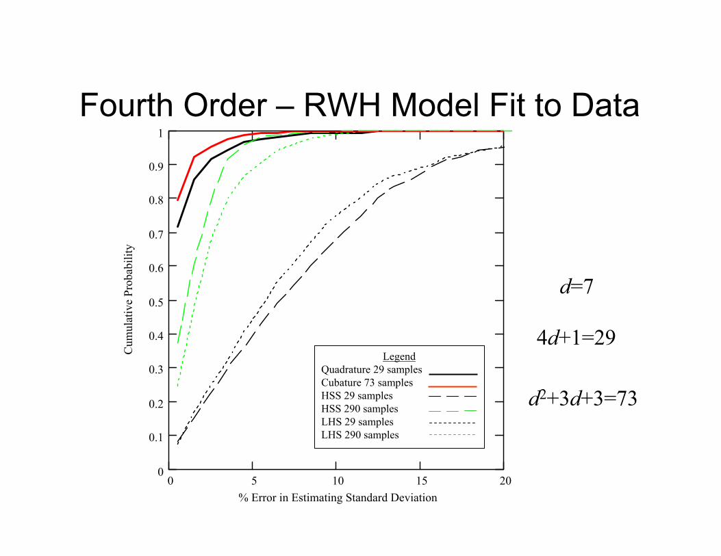
Fourth Order – RWH Model Fit to Data
LegendQuadrature 29 samplesCubature 73 samplesHSS 29 samplesHSS 290 samplesLHS 29 samplesLHS 290 samples
d=7
4d+1=29
d2+3d+3=73
0 5 10 15 200
0.1
0.2
0.3
0.4
0.5
0.6
0.7
0.8
0.9
1
% Error in Estimating Standard Deviation
Cum
ulat
ive
Prob
abili
ty
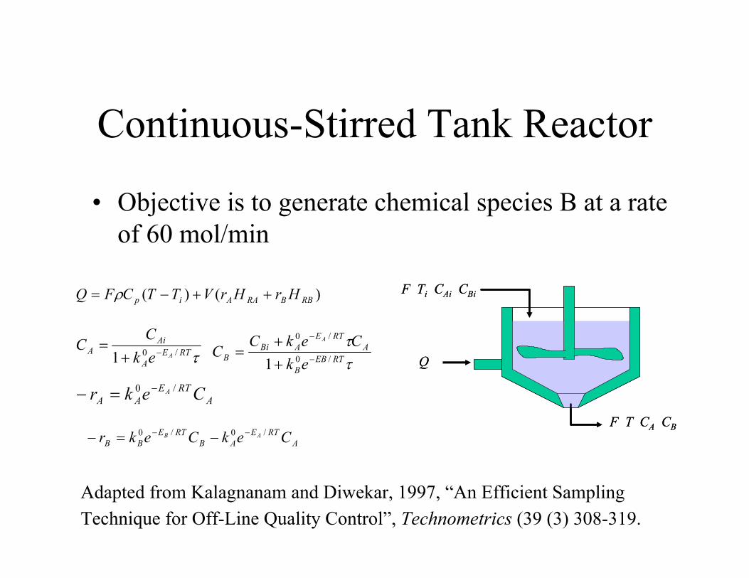
Continuous-Stirred Tank Reactor
• Objective is to generate chemical species B at a rate of 60 mol/min
)()( RBBRAAip HrHrVTTCFQ
RTEA
AiA Aek
CC /01 RTEB
B
ARTE
ABiB ek
CekCC
A
/0
/0
1
ARTE
AA Cekr A /0
ARTE
ABRTE
BB CekCekr AB /0/0
Q
F Ti CAi CBi
F T CA CB
Q
F Ti CAi CBi
F T CA CB
Adapted from Kalagnanam and Diwekar, 1997, “An Efficient Sampling Technique for Off-Line Quality Control”, Technometrics (39 (3) 308-319.
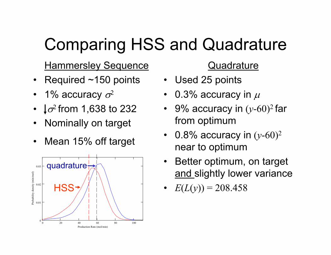
Comparing HSS and QuadratureHammersley Sequence
• Required ~150 points• 1% accuracy 2
• 2 from 1,638 to 232• Nominally on target
• Mean 15% off target
Quadrature• Used 25 points• 0.3% accuracy in• 9% accuracy in (y-60)2 far
from optimum• 0.8% accuracy in (y-60)2
near to optimum• Better optimum, on target
and slightly lower variance• E(L(y)) = 208.458
0 20 40 60 80 1000
0.01
0.02
0.03
Production Rate (mol/min)
Prob
abili
ty d
ensi
ty (m
in/m
ol)
HSS
quadrature
Plan for the Session
• Basic concepts in probability and statistics• Review design of experiments• Basics of Robust Design• Research topics
– Model-based assessment of RD methods – Faster computer-based robust design– Robust invention
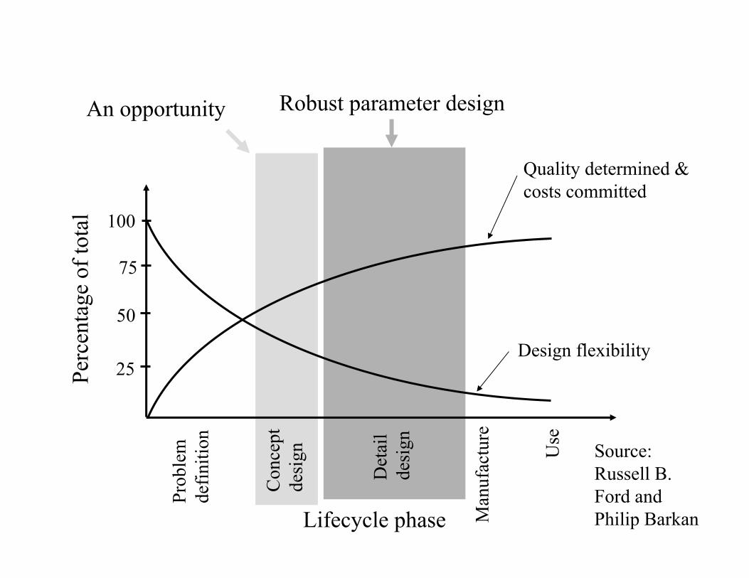
Prob
lem
defin
ition
Con
cept
desi
gn
Det
ail
desi
gn
Man
ufac
ture
Use
Perc
enta
ge o
f tot
al 100
50
75
25
Quality determined & costs committed
Design flexibility
Lifecycle phase
Source:Russell B. Ford and Philip Barkan
Robust parameter designAn opportunity

Defining “Robustness Invention”
• A “robustness invention” is a technical or design innovation whose primary purpose is to make performance more consistent despite the influence of noise factors
• The patent summary and prior art sections usually provide clues
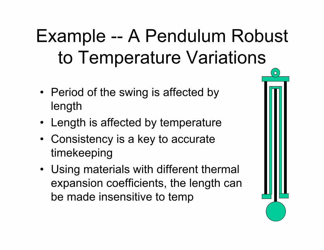
Example -- A Pendulum Robust to Temperature Variations
• Period of the swing is affected by length
• Length is affected by temperature• Consistency is a key to accurate
timekeeping• Using materials with different thermal
expansion coefficients, the length can be made insensitive to temp
Theory of Inventive Problem Solving (TRIZ)
• Genrich Altshuller sought to identify patterns in the patent literature
• Defined problems as contradictions• Provided a large database of solutions • Stimulate designer’s creativity by
presenting past designs appropriate to their current challenge
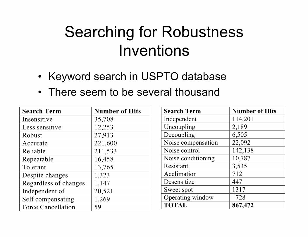
Searching for Robustness Inventions
• Keyword search in USPTO database• There seem to be several thousand
Search Term Number of Hits Independent 114,201 Uncoupling 2,189 Decoupling 6,505 Noise compensation 22,092 Noise control 142,138 Noise conditioning 10,787 Resistant 3,535 Acclimation 712 Desensitize 447 Sweet spot 1317 Operating window 728 TOTAL 867,472
Search Term Number of Hits Insensitive 35,708 Less sensitive 12,253 Robust 27,913 Accurate 221,600 Reliable 211,533 Repeatable 16,458 Tolerant 13,765 Despite changes 1,323 Regardless of changes 1,147 Independent of 20,521 Self compensating 1,269 Force Cancellation 59
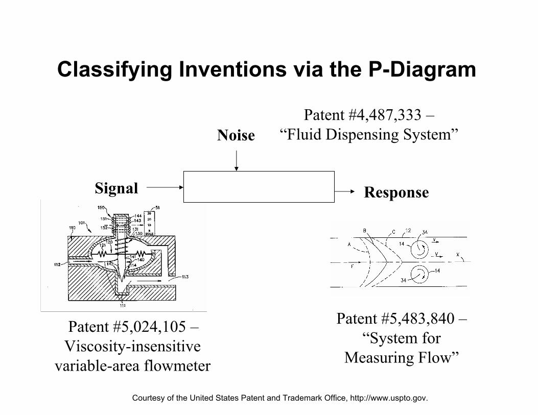
Signal Response
Noise
Classifying Inventions via the P-Diagram
Patent #5,024,105 –Viscosity-insensitive
variable-area flowmeter
Patent #5,483,840 –“System for
Measuring Flow”
Patent #4,487,333 –“Fluid Dispensing System”
Courtesy of the United States Patent and Trademark Office, http://www.uspto.gov.��

Discussion Point
Ball
RampFunnel
Response =the time the ball remains in the funnel
Noise Factor = 2 Types of Ball
Name some ways that you might modify the ball and ramp equipment or procedure to make the system robust to ball type.
Conclusions So Far• Effective strategies for experimentation
should be adaptive (not always, but under a broad range of scenarios)
• Resolution is not always required for reliable improvement
• Simulating the process of experimentation provides insights I can’t get from deduction alone

Questions?
Dan FreyAssistant Professor of Mechanical Engineering and Engineering Systems