MSE 490 Research Final Report

Effects of Pulling Velocity on Solidification of SCN-DC Eutectic System

Zhenjie Yao ycollin@umich.edu Robert Spurney rgspurn@umich.edu

Introduction

A study of directional-growth of succinonitrile–(D)camphor (SCN–DC) at eutectic concentration in thin and bulk samples using real-time observation methods had been done by S. Akamatsu et al [1]. The results show the growth of rod-like patterns in the bulk sample; and prove that 𝜆!! 𝑉=constant, where 𝜆! is the minimum-undercooling spacing and 𝑉 is the pulling velocity. Dynamical studies of solidification microstructures require real-time observations of the solid-liquid interface during lamellar or rod growth. This kind of observation is better performed with optical methods using transparent, nonfaceted organic alloys, such as SCN-DC and Succinonitrile-Nitropentyl glycol (SCN-NPG). In the SCN-DC system, the volume fraction of phases favors rod growth. However, this study is focused on thin-film growth, so the resulting growth will be more lamellar in structure.

This research focuses on the computational simulation of the solidification behavior of a eutectic system and compares it with experimental observation. A phase field model parameterized for a SCN-DC eutectic system is developed to simulate the difference in solidification dynamics between speed-up and slow-down of pulling velocity for a thin SCN-DC film on a moving temperature-gradient stage. The effect of the changes in undercooling on the lamellar spacing and solidification behavior is discussed and compared with experimental results for a similar SCN-NPG system.

Model

Literature Background

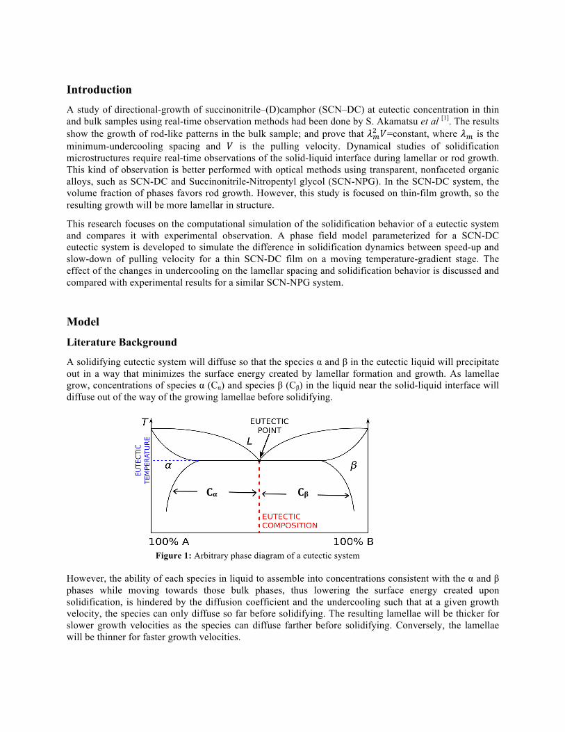
A solidifying eutectic system will diffuse so that the species α and β in the eutectic liquid will precipitate out in a way that minimizes the surface energy created by lamellar formation and growth. As lamellae grow, concentrations of species α (Cα) and species β (Cβ) in the liquid near the solid-liquid interface will diffuse out of the way of the growing lamellae before solidifying.

Figure 1: Arbitrary phase diagram of a eutectic system However, the ability of each species in liquid to assemble into concentrations consistent with the α and β phases while moving towards those bulk phases, thus lowering the surface energy created upon solidification, is hindered by the diffusion coefficient and the undercooling such that at a given growth velocity, the species can only diffuse so far before solidifying. The resulting lamellae will be thicker for slower growth velocities as the species can diffuse farther before solidifying. Conversely, the lamellae will be thinner for faster growth velocities.

Cβ Cα

Although the lamellar structure will not be formed when the rod minimum undercooling is lower than that for lamellae, it is evident that the rod minimum undercooling represents a stabilizing influence on the lamellar structure. Jackson et al proved that the steady-state solution for the diffusion equation is similar for the rod-type eutectic system [2]. The average curvature of the interface depends on the angles at the phase boundaries and on the rod spacing. For the 𝛼 phase in a 𝛽 matrix, the curvature for  𝛼 phase and 𝛽 phase, respectively, is:

!!!

= !!!sin 𝜃! (1a)

!!!

= !!!(!!!!!)!!!!!

sin 𝜃! (1b)

where 𝜌! and 𝜌! are the curvature, 𝑟! and 𝑟! are the radii, and the 𝜃! and 𝜃! are the interface angles for 𝛼 phase and 𝛽 phase respectively.

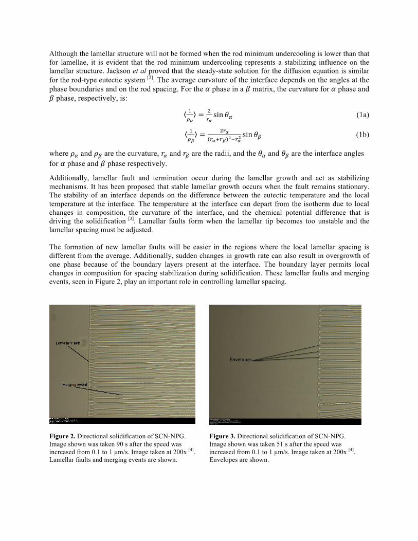
Additionally, lamellar fault and termination occur during the lamellar growth and act as stabilizing mechanisms. It has been proposed that stable lamellar growth occurs when the fault remains stationary. The stability of an interface depends on the difference between the eutectic temperature and the local temperature at the interface. The temperature at the interface can depart from the isotherm due to local changes in composition, the curvature of the interface, and the chemical potential difference that is driving the solidification [3]. Lamellar faults form when the lamellar tip becomes too unstable and the lamellar spacing must be adjusted. The formation of new lamellar faults will be easier in the regions where the local lamellar spacing is different from the average. Additionally, sudden changes in growth rate can also result in overgrowth of one phase because of the boundary layers present at the interface. The boundary layer permits local changes in composition for spacing stabilization during solidification. These lamellar faults and merging events, seen in Figure 2, play an important role in controlling lamellar spacing.

Figure 2. Directional solidification of SCN-NPG. Image shown was taken 90 s after the speed was increased from 0.1 to 1 µm/s. Image taken at 200x [4]. Lamellar faults and merging events are shown.

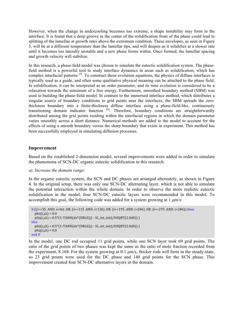
Figure 3. Directional solidification of SCN-NPG. Image shown was taken 51 s after the speed was increased from 0.1 to 1 µm/s. Image taken at 200x [4]. Envelopes are shown.

if  ((i>=35  .AND.  i<46)  .OR.  (i>=115  .AND.  i<126)  .OR.  (i>=195  .AND.  i<206)  .OR.  (i>=275  .AND.  i<286))  then        phii(i,j,k)  =  0.0        phij(i,j,k)  =  0.5*(1-­‐TANH(dx*(DBLE(j)  -­‐  SL_int_init)/DSQRT(2.0d0))  )     else        phii(i,j,k)  =  0.5*(1-­‐TANH(dx*(DBLE(j)  -­‐  SL_int_init)/DSQRT(2.0d0))  )        phij(i,j,k)  =  0.0 end  if

However, when the change in undercooling becomes too extreme, a shape instability may form in the interface. It is found that a deep groove in the center of the solidification front of the phase could lead to splitting of the lamellae at growth rates above the extremum condition. These envelopes, as seen in Figure 3, will be at a different temperature than the lamellar tips, and will deepen as it solidifies at a slower rate until it becomes too laterally unstable and a new phase forms within. Once formed, the lamellar spacing and growth velocity will stabilize.

In this research, a phase-field model was chosen to simulate the eutectic solidification system. The phase-field method is a powerful tool to study interface dynamics in areas such as solidification, which has complex interfacial patterns [5]. To construct these evolution equations, the physics of diffuse interfaces is typically used as a guide, and often some qualitative physical meaning can be attached to the phase field. In solidification, it can be interpreted as an order parameter, and its time evolution is considered to be a relaxation towards the minimum of a free energy. Furthermore, smoothed boundary method (SBM) was used in building the phase-field model. In contrast to the immersed interface method, which distributes a singular source of boundary conditions to grid points near the interfaces, the SBM spreads the zero-thickness boundary into a finite-thickness diffuse interface using a phase-field-like, continuously transitioning domain indicator function [6]. Therefore, boundary conditions are straightforwardly distributed among the grid points residing within the interfacial regions in which the domain parameter varies smoothly across a short distance. Numerical methods are added to the model to account for the effects of using a smooth boundary versus the sharp boundary that exists in experiment. This method has been successfully employed in simulating diffusion processes.

Improvement

Based on the established 2-dimension model, several improvements were added in order to simulate the phenomena of SCN-DC organic eutectic solidification in this research.

a). Increase the domain range:

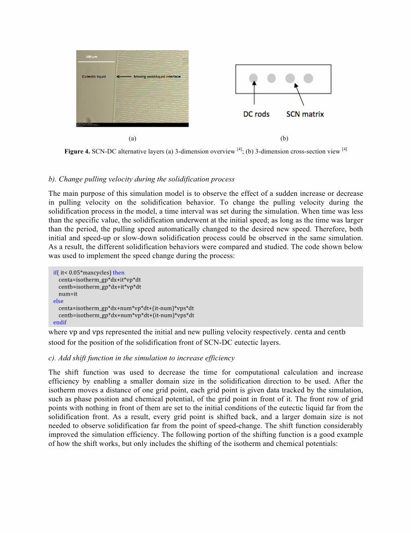
In the organic eutectic system, the SCN and DC phases are arranged alternately, as shown in Figure 4. In the original setup, there was only one SCN-DC alternating layer, which is not able to simulate the potential interaction within the whole domain. In order to observe the more realistic eutectic solidification in the model, four SCN-DC eutectic layers were recommended in this model. To accomplish this goal, the following code was added for a system growing at 1 µm/s:

In the model, one DC rod occupied 11 grid points, while one SCN layer took 69 grid points. The ratio of the grid points of two phases was kept the same as the ratio of mole fraction recorded from the experiment, 8.168. For the system growing at 0.1 µm/s, thicker rods will form in the steady-state, so 23 grid points were used for the DC phase and 140 grid points for the SCN phase. This improvement created four SCN-DC alternative layers in the domain.

if(  it<  0.05*maxcycles)  then        centa=isotherm_gp*dx+it*vp*dt          centb=isotherm_gp*dx+it*vp*dt        num=it else        centa=isotherm_gp*dx+num*vp*dt+(it-­‐num)*vps*dt          centb=isotherm_gp*dx+num*vp*dt+(it-­‐num)*vps*dt endif

(a) (b)

Figure 4. SCN-DC alternative layers (a) 3-dimension overview [4]; (b) 3-dimension cross-section view [4]

b). Change pulling velocity during the solidification process

The main purpose of this simulation model is to observe the effect of a sudden increase or decrease in pulling velocity on the solidification behavior. To change the pulling velocity during the solidification process in the model, a time interval was set during the simulation. When time was less than the specific value, the solidification underwent at the initial speed; as long as the time was larger than the period, the pulling speed automatically changed to the desired new speed. Therefore, both initial and speed-up or slow-down solidification process could be observed in the same simulation. As a result, the different solidification behaviors were compared and studied. The code shown below was used to implement the speed change during the process:

where vp  and vps represented the initial and new pulling velocity respectively. centa and centb stood for the position of the solidification front of SCN-DC eutectic layers.

c). Add shift function in the simulation to increase efficiency

The shift function was used to decrease the time for computational calculation and increase efficiency by enabling a smaller domain size in the solidification direction to be used. After the isotherm moves a distance of one grid point, each grid point is given data tracked by the simulation, such as phase position and chemical potential, of the grid point in front of it. The front row of grid points with nothing in front of them are set to the initial conditions of the eutectic liquid far from the solidification front. As a result, every grid point is shifted back, and a larger domain size is not needed to observe solidification far from the point of speed-change. The shift function considerably improved the simulation efficiency. The following portion of the shifting function is a good example of how the shift works, but only includes the shifting of the isotherm and chemical potentials:

Results

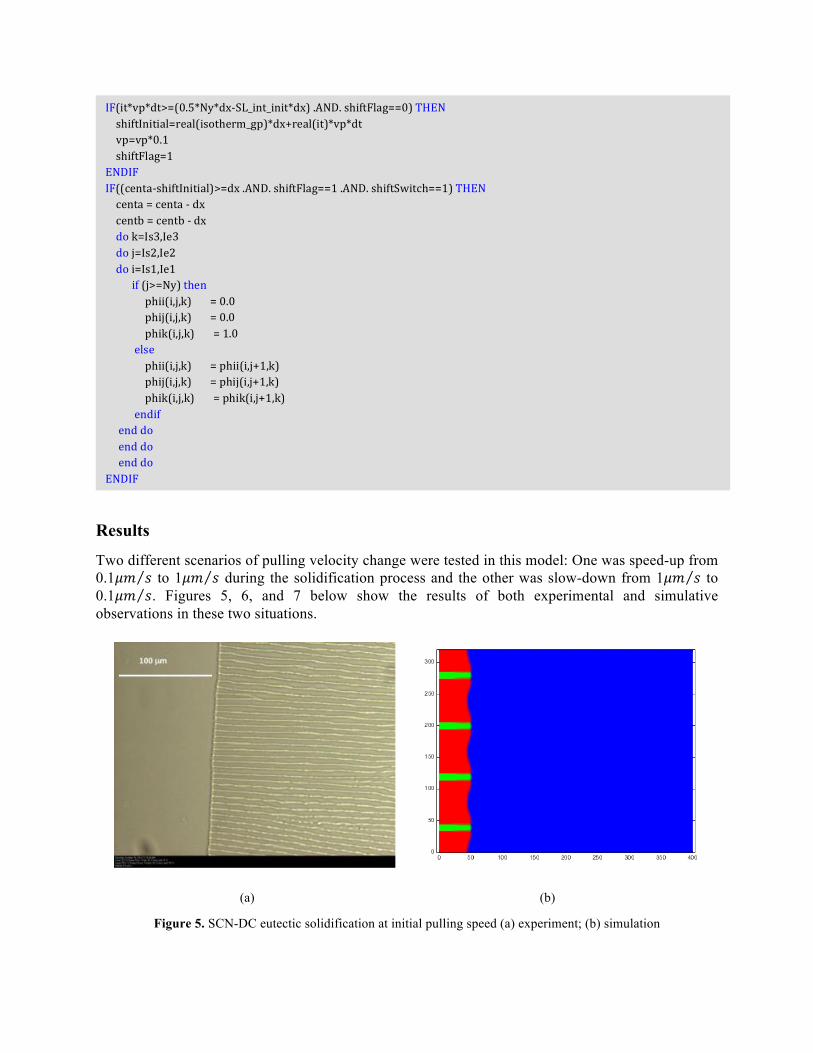
Two different scenarios of pulling velocity change were tested in this model: One was speed-up from 0.1𝜇𝑚 𝑠 to 1𝜇𝑚 𝑠 during the solidification process and the other was slow-down from 1𝜇𝑚 𝑠 to 0.1𝜇𝑚 𝑠. Figures 5, 6, and 7 below show the results of both experimental and simulative observations in these two situations.

(a) (b)

Figure 5. SCN-DC eutectic solidification at initial pulling speed (a) experiment; (b) simulation

IF(it*vp*dt>=(0.5*Ny*dx-­‐SL_int_init*dx)  .AND.  shiftFlag==0)  THEN          shiftInitial=real(isotherm_gp)*dx+real(it)*vp*dt          vp=vp*0.1          shiftFlag=1  ENDIF  IF((centa-­‐shiftInitial)>=dx  .AND.  shiftFlag==1  .AND.  shiftSwitch==1)  THEN                      centa  =  centa  -­‐  dx          centb  =  centb  -­‐  dx          do  k=Is3,Ie3          do  j=Is2,Ie2          do  i=Is1,Ie1                      if  (j>=Ny)  then                                phii(i,j,k)              =  0.0                                phij(i,j,k)              =  0.0                                phik(i,j,k)              =  1.0                        else                                phii(i,j,k)              =  phii(i,j+1,k)                                phij(i,j,k)              =  phij(i,j+1,k)                                phik(i,j,k)              =  phik(i,j+1,k)                        endif            end  do            end  do            end  do  ENDIF  

(a) (b) (c)

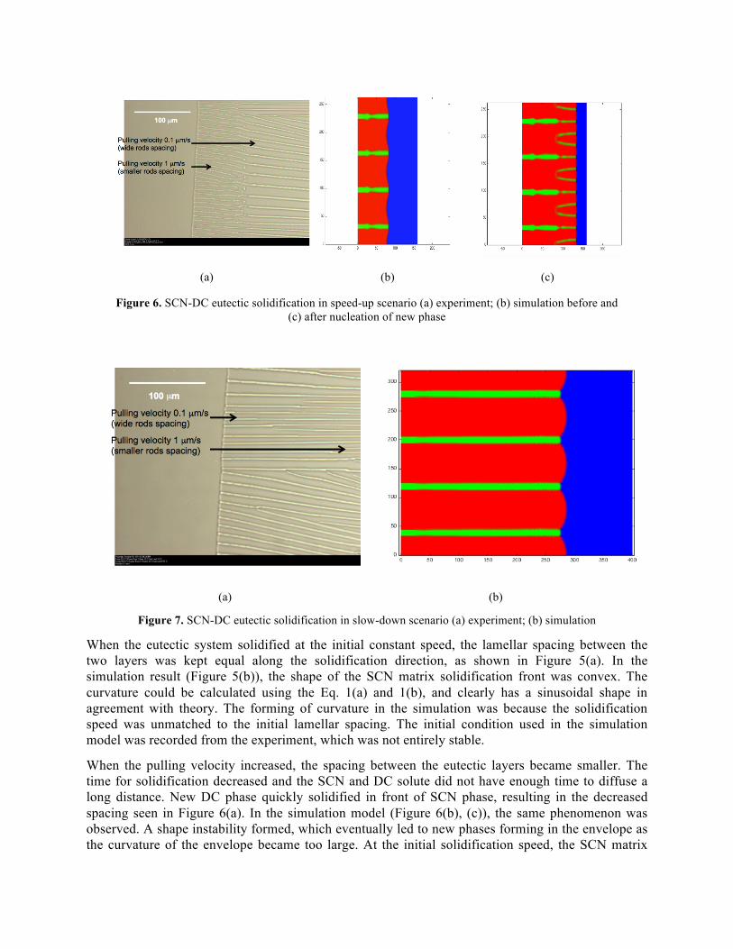
Figure 6. SCN-DC eutectic solidification in speed-up scenario (a) experiment; (b) simulation before and (c) after nucleation of new phase

(a) (b)

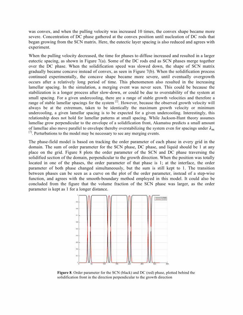
Figure 7. SCN-DC eutectic solidification in slow-down scenario (a) experiment; (b) simulation

When the eutectic system solidified at the initial constant speed, the lamellar spacing between the two layers was kept equal along the solidification direction, as shown in Figure 5(a). In the simulation result (Figure 5(b)), the shape of the SCN matrix solidification front was convex. The curvature could be calculated using the Eq. 1(a) and 1(b), and clearly has a sinusoidal shape in agreement with theory. The forming of curvature in the simulation was because the solidification speed was unmatched to the initial lamellar spacing. The initial condition used in the simulation model was recorded from the experiment, which was not entirely stable.

When the pulling velocity increased, the spacing between the eutectic layers became smaller. The time for solidification decreased and the SCN and DC solute did not have enough time to diffuse a long distance. New DC phase quickly solidified in front of SCN phase, resulting in the decreased spacing seen in Figure 6(a). In the simulation model (Figure 6(b), (c)), the same phenomenon was observed. A shape instability formed, which eventually led to new phases forming in the envelope as the curvature of the envelope became too large. At the initial solidification speed, the SCN matrix

was convex, and when the pulling velocity was increased 10 times, the convex shape became more severe. Concentration of DC phase gathered at the convex position until nucleation of DC rods that began growing from the SCN matrix. Here, the eutectic layer spacing is also reduced and agrees with experiment.

When the pulling velocity decreased, the time for phases to diffuse increased and resulted in a larger eutectic spacing, as shown in Figure 7(a). Some of the DC rods end as SCN phases merge together over the DC phase. When the solidification speed was slowed down, the shape of SCN matrix gradually became concave instead of convex, as seen in Figure 7(b). When the solidification process continued experimentally, the concave shape became more severe, until eventually overgrowth occurs after a relatively long period of time. This phenomenon also resulted in the increasing lamellar spacing. In the simulation, a merging event was never seen. This could be because the stabilization is a longer process after slow-down, or could be due to overstability of the system at small spacing. For a given undercooling, there are a range of stable growth velocities and therefore a range of stable lamellar spacings for the system [2]. However, because the observed growth velocity will always be at the extremum, taken to be identically the maximum growth velocity or minimum undercooling, a given lamellar spacing is to be expected for a given undercooling. Interestingly, this relationship does not hold for lamellar patterns at small spacing. While Jackson-Hunt theory assumes lamellae grow perpendicular to the envelope of a solidification front, Akamatsu predicts a small amount of lamellae also move parallel to envelope thereby overstabilizing the system even for spacings under 𝜆! [7]. Perturbations to the model may be necessary to see any merging events.

The phase-field model is based on tracking the order parameter of each phase in every grid in the domain. The sum of order parameter for the SCN phase, DC phase, and liquid should be 1 at any place on the grid. Figure 8 plots the order parameter of the SCN and DC phase traversing the solidified section of the domain, perpendicular to the growth direction. When the position was totally located in one of the phases, the order parameter of that phase is 1; at the interface, the order parameter of both phase changed simultaneously, but the sum is still kept to 1. The transition between phases can be seen as a curve on the plot of the order parameter, instead of a step-wise function, and agrees with the smooth-boundary method employed in this model. It could also be concluded from the figure that the volume fraction of the SCN phase was larger, as the order parameter is kept as 1 for a longer distance.

Figure 8. Order parameter for the SCN (black) and DC (red) phase, plotted behind the solidification front in the direction perpendicular to the growth direction

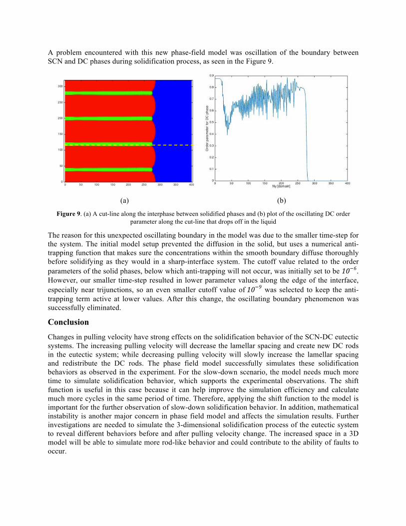
A problem encountered with this new phase-field model was oscillation of the boundary between SCN and DC phases during solidification process, as seen in the Figure 9.

(a) (b)

Figure 9. (a) A cut-line along the interphase between solidified phases and (b) plot of the oscillating DC order parameter along the cut-line that drops off in the liquid

The reason for this unexpected oscillating boundary in the model was due to the smaller time-step for the system. The initial model setup prevented the diffusion in the solid, but uses a numerical anti-trapping function that makes sure the concentrations within the smooth boundary diffuse thoroughly before solidifying as they would in a sharp-interface system. The cutoff value related to the order parameters of the solid phases, below which anti-trapping will not occur, was initially set to be 10!6. However, our smaller time-step resulted in lower parameter values along the edge of the interface, especially near trijunctions, so an even smaller cutoff value of  10!9 was selected to keep the anti-trapping term active at lower values. After this change, the oscillating boundary phenomenon was successfully eliminated.

Conclusion

Changes in pulling velocity have strong effects on the solidification behavior of the SCN-DC eutectic systems. The increasing pulling velocity will decrease the lamellar spacing and create new DC rods in the eutectic system; while decreasing pulling velocity will slowly increase the lamellar spacing and redistribute the DC rods. The phase field model successfully simulates these solidification behaviors as observed in the experiment. For the slow-down scenario, the model needs much more time to simulate solidification behavior, which supports the experimental observations. The shift function is useful in this case because it can help improve the simulation efficiency and calculate much more cycles in the same period of time. Therefore, applying the shift function to the model is important for the further observation of slow-down solidification behavior. In addition, mathematical instability is another major concern in phase field model and affects the simulation results. Further investigations are needed to simulate the 3-dimensional solidification process of the eutectic system to reveal different behaviors before and after pulling velocity change. The increased space in a 3D model will be able to simulate more rod-like behavior and could contribute to the ability of faults to occur.

References [1] S. Akamatsu, et al. Real-time study of thin and bulk eutectic growth in succinonitrile–(D)camphor alloys. Journal of Crystal Growth, 2007, 299, 418–428. [2] K.A.Jackson, and J.D.Hunt. Lamellar and Rod Eutectic Growth. Transactions of the Metallurgical Society of AIME,1996, 236, 1129-1142 [3] F. D. Lemkey, R. W. Hertzberg, and J. A. Ford: Trans. Met. Soc. AIME, 1965, vol. 233, p. 334. [4] Vladislava Tomeckova, Halloran Lab group, University of Michigan, 2015 [5] R. Folch, and M. Plapp. Quantitative phase-field modeling of two-phase solidification. 2007 [6] Hui-Chia Yu, Hsun-Yi Chen and K Thornton. Extended smoothed boundary method for solving partial differential equations with general boundary conditions on complex boundaries. Modelling Simul. Mater. Sci. Eng., 2012, 20, (41pp) [7] S. Akamatsu, M. Plapp, G. Faivre, A. Karma. Overstability of Lamellar Eutectic Growth Below the Minimum Undercooling Spacing. Metallurgical and Materials Transactions A, 2004, 35A, 1815-1828.