MSU Extension Publication Archive Archive copy of publication, do not use for current recommendations. Up-to-date information about many topics can be obtained from your local Extension office. Aids to Professional Forestry Practice Michigan State University Extension Service Robert Marty, Department of Forestry Issued May 1984 21 pages The PDF file was provided courtesy of the Michigan State University Library

Scroll down to view the publication.

Extension Bulletin E-1757, May "1984 " Cooperative Extension Service

Michigan State University $1.00

AIDS TO PROFESSIONAL FORESTRY PRACTICE

M l • • , | , , , ; , • | | • • | • | |

"- ± ± ± ± E T : ^ ^ k V""J *mt yd. *hr i » i r ^ 1 1 m \ m V lT ' T

A • - * m§ 1 m 1 * ml « 1 A p 1 • L # 1 \ m\ _L - 1 . ^ ^ # .m\ * * ]J .1L

O A m JT • » • W ^ ' T # ^ W J\ rLJnujFm 1 m i l w 1 f-% 1 w 1 1 1 1 %l H • V^ZJZ •Ljt-I t J t j t«zJL i: 1 ^t^p

•'L,,k-I iftiSSj1"

'wiSBSRi -%§l ESIiiifcu—' ^ X f S n V ^ f n V' '

—r -f- *2! E^taNlL Bff*l ^ W *talB ||^J8H<fJi*w

i t e l l BnW^Vi ! v,i*4<. i, jjf''S».*^ -̂" »

J x * f ' ' ' . ' , " • •• 01

H L ' ' -JMBto. " ̂ ••,-r3K5*M

(MJK^L 1 rlWaB -̂J MBrTfff ^aBSffit1 tHsisiLPrH S aP^SRSltei*

^ WM* Rm^' i?^^ ' T * n 1 rtMfnfc'rY^ UBL

1 £ ftt^mfw > " ' l^^Mfc ^>

Iw 1 1 I "• •» ROBERT MARTY

DEPARTMENT OF FORESTRY MICHIGAN STATE UNIVERSITY

MICHIGAN STATE UNIVERSITY

CE5 5M-4:84 (New), KMF-LB

EXT°E P N E S"ON I V E Price $1.00, For Sale Only SERVICE

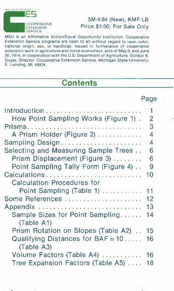
MSU is an Affirmative Action/Equal Opportunity Institution. Cooperative Extension Service programs are open to all without regard to race, color, national origin, sex, or handicap. Issued in furtherance of cooperative extension work in agriculture and home economics, acts of May 8, and June 30,1914, in cooperation with the U.S. Department of Agriculture. Gordon E. Guyer, Director, Cooperative Extension Service, Michigan State University, E. Lansing, Ml 48824.

Contents

Page

Introduction 1 How Point Sampling Works (Figure 1) . 2

Prisms 3 A Prism Holder (Figure 2) 4

Sampling Design 4 Selecting and Measuring Sample Trees . . 6

Prism Displacement (Figure 3) 6 Point Sampling Tally Form (Figure 4) . . 9

Calculations 10 Calculation Procedures for

Point Sampling (Table 1) 11 Some References 12 Appendix 13

Sample Sizes for Point Sampling 14 (Table A1)

Prism Rotation on Slopes (Table A2) . . 15 Qualifying Distances for BAF = 10 16

(Table A3) Volume Factors (Table A4) 16 Tree Expansion Factors (Table A5) . . . . 18

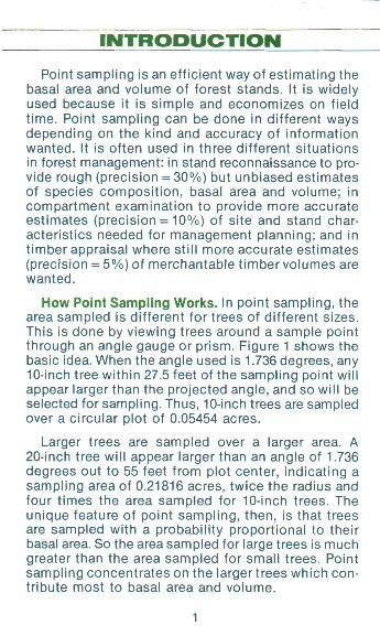
INTRODUCTION Point sampling is an efficient way of estimating the

basal area and volume of forest stands. It is widely used because it is simple and economizes on field time. Point sampling can be done in different ways depending on the kind and accuracy of information wanted. It is often used in three different situations in forest management: in stand reconnaissance to pro­vide rough (precision = 30%) but unbiased estimates of species composition, basal area and volume; in compartment examination to provide more accurate estimates (precision = 10%) of site and stand char­acteristics needed for management planning; and in timber appraisal where still more accurate estimates (precision = 5%) of merchantable timber volumes are wanted.

How Point Sampling Works. In point sampling, the area sampled is different for trees of different sizes. This is done by viewing trees around a sample point through an angle gauge or prism. Figure 1 shows the basic idea. When the angle used is 1.736 degrees, any 10-inch tree within 27.5 feet of the sampling point will appear larger than the projected angle, and so will be selected for sampling. Thus, 10-inch trees are sampled over a circular plot of 0.05454 acres.

Larger trees are sampled over a larger area. A 20-inch tree will appear larger than an angle of 1.736 degrees out to 55 feet from plot center, indicating a sampling area of 0.21816 acres, twice the radius and four times the area sampled for 10-inch trees. The unique feature of point sampling, then, is that trees are sampled with a probability proportional to their basal area. So the area sampled for large trees is much greater than the area sampled for small trees. Point sampling concentrates on the larger trees which con­tribute most to basal area and volume.

1

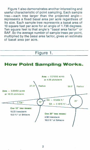
Figure 1 also demonstrates another interesting and useful characteristic of point sampling. Each sample tree—each tree larger than the projected a n g l e -represents a fixed basal area per acre regardless of its size. Each sample tree represents a basal area of 10 square feet per acre for an angle of 1.736 degrees. Ten square feet is that angle's "basal area factor" or BAF. So the average number of sample trees per point, multiplied by the basal area factor, gives an estimate of basal area per acre.

Figure 1

H o w Point Sampl ing Works .

Area = 0.21816 acres

or 4.58 plots/acre

2 7 . 5 ' \ Radius 55.0' \ Radius

Area = 0.05454 acres

or 18.33 plots/acre

10" ilc- BA = 0.5454 ft.2

BA = 2.1816 ft.

One 10" tree means:

18.33 trees/acre

10.0 ft.2 of BA/acre One 20" tree means:

4.58 trees/acre

10.0 ft.2 of BA/acre

2

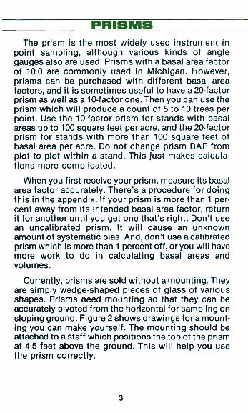
PRISMS The prism is the most widely used instrument in

point sampling, although various kinds of angle gauges also are used. Prisms with a basal area factor of 10.0 are commonly used in Michigan. However, prisms can be purchased with different basal area factors, and it is sometimes useful to have a 20-factor prism as well as a 10-factor one. Then you can use the prism which will produce a count of 5 to 10 trees per point. Use the 10-factor prism for stands with basal areas up to 100 square feet per acre, and the 20-factor prism for stands with more than 100 square feet of basal area per acre. Do not change prism BAF from plot to plot within a stand. This just makes calcula­tions more complicated.

When you first receive your prism, measure its basal area factor accurately. There's a procedure for doing this in the appendix. If your prism is more than 1 per­cent away from its intended basal area factor, return it for another until you get one that's right. Don't use an uncalibrated prism. It will cause an unknown amount of systematic bias. And, don't use a calibrated prism which is more than 1 percent off, or you will have more work to do in calculating basal areas and volumes.

Currently, prisms are sold without a mounting. They are simply wedge-shaped pieces of glass of various shapes. Prisms need mounting so that they can be accurately pivoted from the horizontal for sampling on sloping ground. Figure 2 shows drawings for a mount­ing you can make yourself. The mounting should be attached to a staff which positions the top of the prism at 4.5 feet above the ground. This will help you use the prism correctly.

3

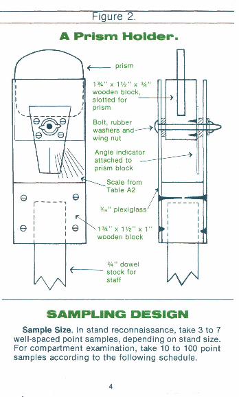
Figure 2.

A P r i s m H o l d e r .

prism

1 % " x V/z" x 3/4' wooden block, slotted for prism

Bolt, rubber washers and-—' wing nut

Angle indicator attached to prism block

Scale from Table A2

yie" plexiglass

13 /4" X 1 V 2 " X V

wooden block

3/4" dowel stock for staff

•C

•«l

iv4

>

SAMPLING DESIGN Sample Size. In stand reconnaissance, take 3 to 7

well-spaced point samples, depending on stand size. For compartment examination, take 10 to 100 point samples according to the following schedule.

4

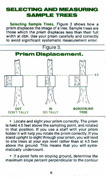
Size of Stand Number of Sampling Points

acres

0-10 11- 40 41- 80 81-240 240 +

10 1 point per acre

40 + (acres - 40)/2 60 + (acres - 80)/4

100

This schedule usually will provide a 10 percent preci­sion of estimate, at the 90 percent confidence inter­val, for stands of 40 acres or more. You must take approximately four times this number of samples if you wish to achieve a 95 percent confidence interval. See the appendix for more on sample size.

Locating Sample Points. Sample points can be located randomly or systematically within the stand. However, systematic sampling usually is used because it is easier and less time consuming. Sample points are evenly spaced along parallel cruise lines oriented to cross contour lines approximately at right angles. This provides a distribution of sample points which have a good chance of encountering varying stand conditions in proportion to their occurrence.

Sampling studies indicate that systematically located points usually provide estimates with equal or even greater precision than an equal number of random sample points. So, random sampling formulas for calculating sampling means and variances are commonly applied to systematic samples, even though the statistical assumptions of random sampl­ing are not met.

All plots should be located at least one chain from stand boundaries to avoid edge bias. Edge bias occurs when a point is located close enough to a stand bound­ary so that part of the area sampled falls outside the stand. c

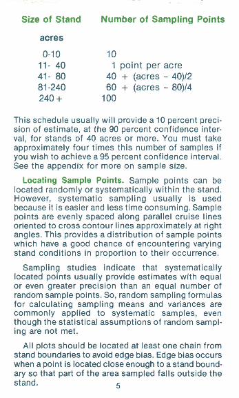
SELECTING AND MEASURING SAMPLE TREES

Selecting Sample Trees. Figure 3 shows how a prism displaces the image of a tree. Sample trees are those which the prism displaces less than their full width at dbh. Use your prism carefully and correctly to avoid significant systematic measurement error:

Figure 3.

Itii

P r i s m D i s i

< u

ii

1 ^

1

i

•:: 11

i ]

''A

a c e m e m

^

||i,ll

i

t .

1 ' 1

:, li

*

>

- , - - 4 5'

I OUT IN BORDERLINE

DON'T TALLY DO TALLY TREE

• Locate and sight your prism correctly. The prism is held 4.5 feet above the sampling point, and rotated in that position. If you use a staff with your prism holder it will help you rotate the prism correctly. If you stand upright to sight through your prism, you will tend to site trees at your eye level rather than at 4.5 feet above the ground. This means that you will syste­matically undercount.

• If a point falls on sloping ground, determine the maximum slope percent perpendicular to the contour

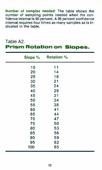
through the sampling point. Then pivot your prism from the horizontal by the percent indicated in appen­dix Table A2. If you make a prism holder like the one in Figure 2, you can set the necessary prism angle directly from the slope percent reading. Pivoting the prism reduces its basal area factor and gives an en­larged sampling circle on the slope. This projects to a horizontal elipse of the proper sampling area. Make this adjustment for points with slopes of 15 percent or more.

• Sometimes, it's hard to tell whether a tree should be counted or not. In stand reconnaissance, simply count every second borderline tree. However, in sampling where more accuracy is needed, measure the distance on the ground between the sampling point and the midpoint of the borderline tree. Then measure its dbh, and refer to appendix Table A3 to see whether it should be counted. This same procedure can be used for leaning or fallen trees by measuring to where the midpoint of the tree would be if it were upright. If you do not measure borderline trees, you will con­sistently undercount.

• Be sure to check for trees which are hidden or masked by other trees closer to the sampling point. Move away from the sampling point on an arc to check masked trees.

• Sometimes the same large tree will be a sample tree from two separate sampling points. That's ok. It should be counted at both points.

Measuring Sample Trees. Sample tree measure­ments depend on the information needed. Part of cruise planning is to determine exactly what site and stand characteristics are needed. Don't go out in the woods until you've decided. Here are the measure­ments you need to estimate various site and stand characteristics.

• Basal Area: count the number of sample trees at 7

each sampling point. • Species Composition: record the species or

species group of each sample tree. • Number of Trees per Acre and Diameter Distribu­

tion: measure the dbh class of each sample tree. If there are 40 points or more, dbh can be recorded at every second point.

• Total Cubic Foot Volume of Stemwood: measure the total height of the dominant or codominant tree closest to each sampling point.

• Site Index and Main Stand Age: record the age at dbh and the total height of ttie dominant or codomi­nant tree closest to every nth sampling point, so that 5-10 trees are measured.

• Merchantable Volume: estimate by eye the mer­chantable length of each sample tree, in 16-foot sawlogs and half logs, or in 8-foot pulpwood bolts. If the cruise is for timber appraisal, measure Girard form class and estimate cull percent for the merchantable tree closest to each sampling point.

• Stand Growth Rate: measure dbh and 5-year radial growth for each sample tree. If there are 40 points or more, these measurements can be made at every second point.

Measurements of diameter and radial growth are time consuming and should not be done routinely. These measurements must be taken if you wish to make a stand table projection. However, secondary sources of growth information (such as yield tables and functions that do not require individual tree data), usually are available and will provide a reasonably accurate estimate of stand growth rate. Also, if the stand has been measured before, a comparison of stand volume "then" with stand volume "now" pro­vides the best estimate of periodic stand growth. A convenient tally form for point sampling is shown in Figure 4.

8

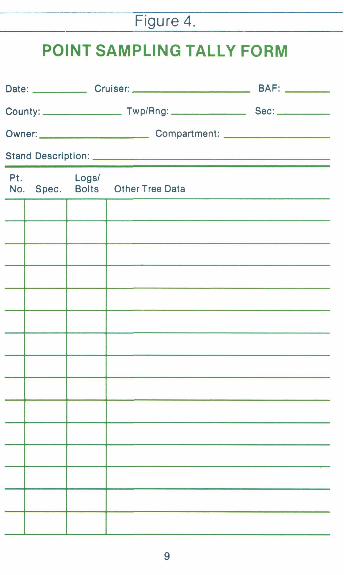
Figure 4.

POINT SAMPLING TALLY FORM

Date: Cruiser: BAF: _

County: Twp/Rng: Sec:

Owner: Compartment:

Stand Description:

Pt. Logs/ No. Spec. Bolts Other Tree Data

9

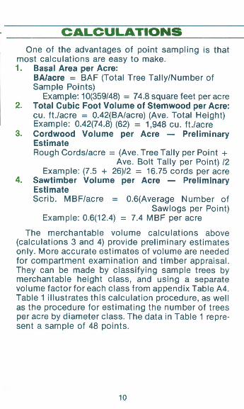
CALCULATIONS One of the advantages of point sampling is that

most calculations are easy to make. 1 . Basal Area per Acre:

BA/acre = BAF (Total Tree Tally/Number of Sample Points)

Example: 10(359/48) = 74.8 square feet per acre 2. Total Cubic Foot Volume of Stemwood per Acre:

cu. ft./acre = 0.42(BA/acre) (Ave. Total Height) Example: 0.42(74.8) (62) = 1,948 cu. ft./acre

3. Cordwood Volume per Acre — Preliminary Estimate Rough Cords/acre = (Ave. Tree Tally per Point +

Ave. Bolt Tally per Point) 12 Example: (7.5 + 26)/2 = 16.75 cords per acre

4. Sawtimber Volume per Acre — Preliminary Estimate Scrib. MBF/acre = 0.6(Average Number of

Sawlogs per Point) Example: 0.6(12.4) = 7.4 MBF per acre

The merchantable volume calculations above (calculations 3 and 4) provide preliminary estimates only. More accurate estimates of volume are needed for compartment examination and timber appraisal. They can be made by classifying sample trees by merchantable height class, and using a separate volume factor for each class from appendix Table A4. Table 1 illustrates this calculation procedure, as well as the procedure for estimating the number of trees per acre by diameter class. The data in Table 1 repre­sent a sample of 48 points.

10

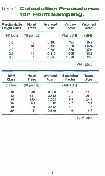
Table 1. Calculat ion P r o c e d u r e s fo r Point Sampl ing.

Merchantable Height Class

No. of Trees

Average/ Point

Volume Factor

Volumes/ Acre

>' logs)

1.0 1.5 2.0 2.5 3.0

(48 points)

43 184 110 15 7

0.896 3.833 2.292 0.312 0.146

(Table A4)

750 1,050 1,350 1,600 1,870

(Mbf)

672 4,024 3,094

502 273

Total 8,565

DBH Class

No. of Trees

Average/ Point

Expansion Factor

Trees/ Acre

(inches)

10 12 14 16 18 20

(48 points)

40 111 123 63 15 7

0.833 2.312 2.562 1.312 0.312 0.146

(Table A5)

18.3 12.7 9.4 7.2 5.7 4.6

Total

15.2 29.4 24.1 9.4 1.8 0.7

80.6

11

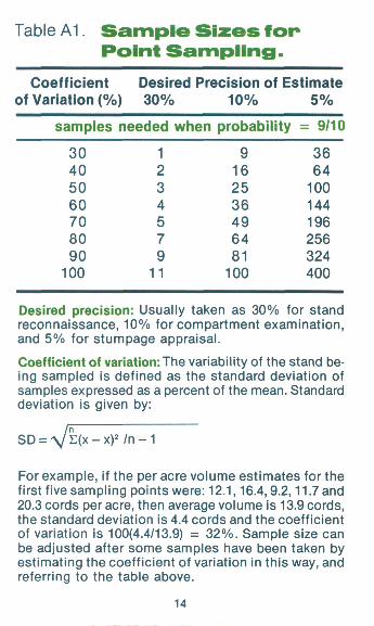
Table A1. S a m p l e S i z e s f o r P o i n t S a m p l i n g .

Coefficient Desired Precision of Estimate of Variation (%) 30% 10% 5%

samples needed when probability = 9/10

30 40 50 60 70 80 90 100

1 2 3 4 5 7 9 11

9 16 25 36 49 64 81 100

36 64 100 144 196 256 324 400

Desired precision: Usually taken as 30% for stand reconnaissance, 10% for compartment examination, and 5% for stumpage appraisal.

Coefficient of variation: The variability of the stand be­ing sampled is defined as the standard deviation of samples expressed as a percent of the mean. Standard deviation is given by:

SD = \Ji(x - x)2 /n - 1

For example, if the per acre volume estimates for the first five sampling points were: 12.1,16.4,9.2,11.7 and 20.3 cords per acre, then average volume is 13.9 cords, the standard deviation is 4.4 cords and the coefficient of variation is 100(4.4/13.9) = 32%. Sample size can be adjusted after some samples have been taken by estimating the coefficient of variation in this way, and referring to the table above.

14

Number of samples needed: The table shows the number of sampling points needed when the con­fidence interval is 90 percent. A 95 percent confidence interval requires four times as many samples as is in­dicated in the table.

Table A2. Prism Rotation on Slopes.

Slope % Rotation %

15 20 25 30 35 40 45 50 55 60 65 70 75 80 85 90 95 100

11 14 18 21 24 28 31 34 38 41 44 47 50 53 56 59 62 65

15

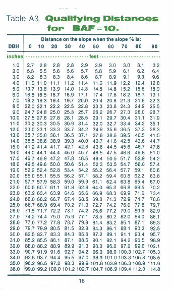
Table A3. Qualifying D is tances f o r BAF = 10.

Distance on the slope when the slope % is: 0 10 20 30 40 50 60 70 80 90

feet

2.7 5.5 8.2

11.0 13.7 16.5 19.2 22.0 24.7 27.5 30.2 33.0 35.7 38.5 41.2 44.0 46.7 49.5 52.2 55.0 57.7 60.5 63.2 66.0 68.7 71.5 74.2 77.0 79.7 82.5 85.2 88.0 90.7 93.5 96.2 99.0

2.8 5.5 8.3

11.0 13.8 16.5 19.3 22.1 24.8 27.6 30.3 33.1 35.8 38.6 41.4 44.1

2.8 5.6 8.3

11.1 13.9 16.7 19.4 22.2 25.0 27.8 30.5 33.3 36.1 38.9 41.7 44.4

46.9 47.2 49.6 50.0 52.4 55.1 57.9 60.7 63.4

52.8 55.5 58.3 61.1 63.9

66.2 66.7 68.9 69.4 71.7 74.4 77.2 79.9 82.7 85.5 88.2 91.9 93.7 96.5

72.2 75.0 77.8 80.5 83.3 86.1 88.9 91.6 94.4 97.2

99.2100.0

2.8 5.6 8.4

11.2 14.0 16.9 19.7 22.5 25.3 28.1 30.9 33.7 36.5 39.3 42.1 45.0 47.8 50.6 53.4 56.2 59.0 61.8 64.6 67.4 70.2 73.1 75.9 78.7 81.5 84.3 87.1 89.9 92.7 95.5 98.3

101.2

2.9 5.7 8.6

11.4 14.3 17.1 20.0 22.8 25.7 28.5 31.4 34.2 37.1 40.0 42.8 45.7 48.5 51.4 54.2 57.1 59.9 62.8 65.6 68.5 71.3 74.2 77.1 79.9 82.8 85.6 88.5 91.3 94.2 97.0 99.9

102.7

2.9 5.8 8.7

11.6 14.5 17.4 20.4 23.3 26.2 29.1 32.0 34.9 37.8 40.7 43.6 46.5 49.4 52.3 55.2 58.2 61.1 64.0 66.9 69.8 72.7 75.6 78.5 81.4 84.3 87.2 90.1 93.0 96.0 98.9

101.8 104,7

3.0 5.9 8.9

11.9 14.8 17.8 20.8 23.8 26.7 29.7 32.7 35.6 38.6 41.6 44.5 47.5 50.5 53.5 56.4 59.4 62.4 65.3 68.3 71.3 74.2 77.2 80.2 83.2 86.1 89.1 92.1 95.0 98.0

101.0 103.9 106.9

3.0 6.1 9.1

12.2 15.2 18.2 21.3 24.3 27.3 30.4 33.4 36.5 39.5 42.5 45.6 48.6 51.7 54.7 57.7 60.8 63.8 66.8 69.9 72.9 76.0 79.0 82.0 85.1 88.1 91.1 94.2 97.2

100.3 103.3 106.3 109.4

3.1 6.2 9.3

12.4 15.6 18.7 21.8 24.9 28.0 31.1 34.2 37.3 40.5 43.6 46.7 49.8 52.9 56.0 59.1 62.2 65.4 68.5 71.6 74.7 77.8 80.9 84.0 87.1 90.2 93.4 96.5 99.6

102.7 105.8 108.9 112.0

3.2 6.4 9.6

12.8 15.9 19.1 22.3 25.5 28.7 31.9 35.1 38.3 41.5 44.7 47.8 51.0 54.2 57.4 60.6 63.8 67.0 70.2 73.4 76.6 79.7 82.9 86.1 89.3 92.5 95.7 98.9

102.1 105.3 108.5 111.6 114.8

16

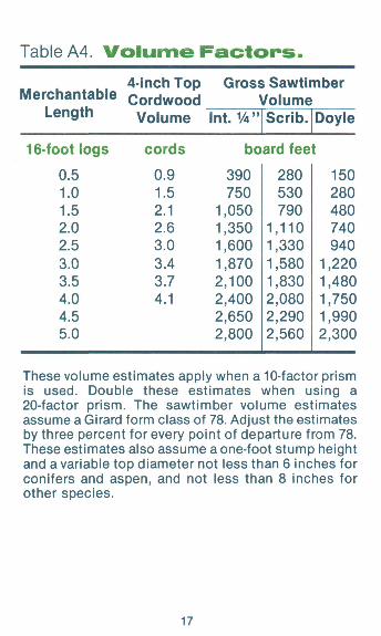
Table A4. Vo lume F a c t o r s . 4-inch Top Gross Sawtimber

Merchantable cordwood Volume Length Volume Int. VA" Scrib. Doyle

16-foot logs cords board feet

0.5 1.0 1.5 2.0 2.5 3.0 3.5 4.0 4.5 5.0

0.9 1.5 2.1 2.6 3.0 3.4 3.7 4.1

390 750

1,050 1,350 1,600 1,870 2,100 2,400 2,650 2,800

280 530 790

1,110 1,330 1,580 1,830 2,080 2,290 2,560

150 280 480 740 940

1,220 1,480 1,750 1,990 2,300

These volume estimates apply when a 10-factor prism is used. Double these estimates when using a 20-factor prism. The sawtimber volume estimates assume a Girard form class of 78. Adjust the estimates by three percent for every point of departure from 78. These estimates also assume a one-foot stump height and a variable top diameter not less than 6 inches for conifers and aspen, and not less than 8 inches for other species.

17

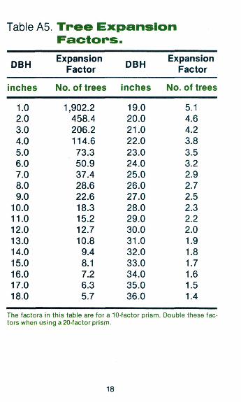
Table A5. T r e e Expansion F a c t o r s .

DBH

inches

1.0 2.0 3.0 4.0 5.0 6.0 7.0 8.0 9.0

10.0 11.0 12.0 13.0 14.0 15.0 16.0 17.0 18.0

Expansion Factor

No. of trees

1,902.2 458.4 206.2 114.6 73.3 50.9 37.4 28.6 22.6 18.3 15.2 12.7 10.8 9.4 8.1 7.2 6.3 5.7

DBH

inches

19.0 20.0 21.0 22.0 23.0 24.0 25.0 26.0 27.0 28.0 29.0 30.0 31.0 32.0 33.0 34.0 35.0 36.0

Expansion Factor

No. of trees

5.1 4.6 4.2 3.8 3.5 3.2 2.9 2.7 2.5 2.3 2.2 2.0 1.9 1.8 1.7 1.6 1.5 1.4

The factors in this table are for a 10-factor prism. Double these fac­tors when using a 20-factor prism.

18

NOTES

NOTES

NOTES