multi-axis tabular loads in ansys workbench - · pdf filemm/dd/yy 2 • users of ansys...
TRANSCRIPT

mm/dd/yy
1
Multi-Axis Tabular Loads
in ANSYS Workbench
2/24/2017

mm/dd/yy
2
• Users of ANSYS Workbench (18) may have noticed
that the they have a choice of independent variables
when defining a tabular load
• Typical choices are Time (the default), X, Y, and Z. If
the choice is time, the number of table entries is
equal to the number of load steps
mm/dd/yy
3
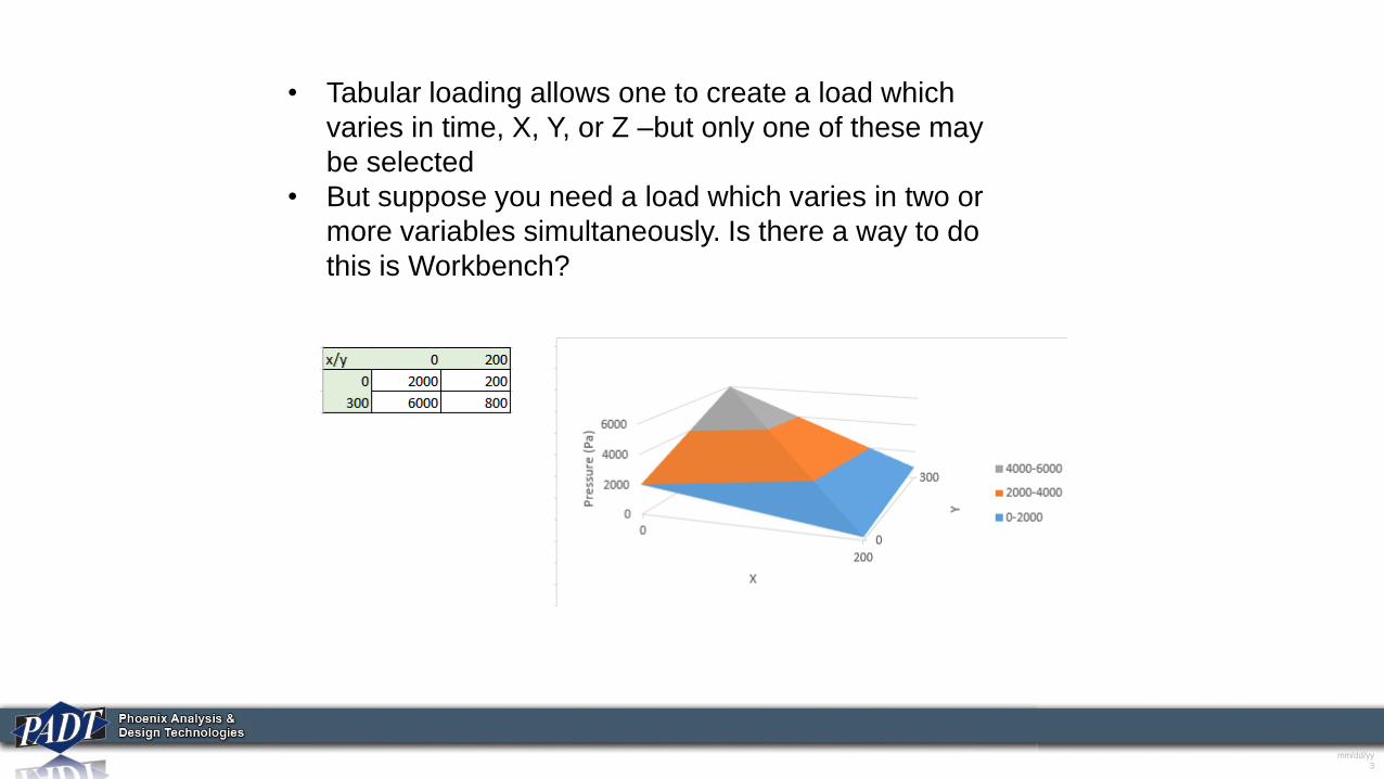
• Tabular loading allows one to create a load which
varies in time, X, Y, or Z –but only one of these may
be selected
• But suppose you need a load which varies in two or
more variables simultaneously. Is there a way to do
this is Workbench?

mm/dd/yy
4
• The standard approach in Workbench is to read the
tabular data from a text file. This is done in the
‘External Data’ tool. Simply drag and drop an External
Data object onto the ‘setup’ cell of your analysis.
mm/dd/yy
5
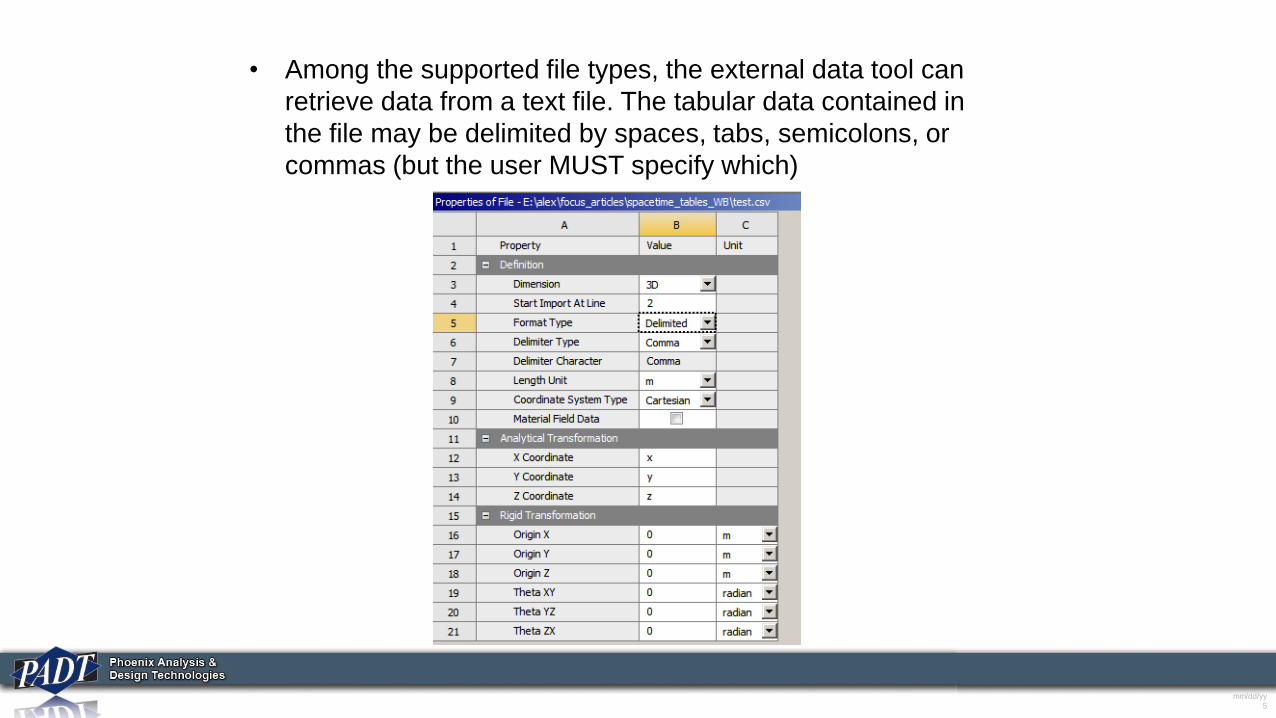
• Among the supported file types, the external data tool can
retrieve data from a text file. The tabular data contained in
the file may be delimited by spaces, tabs, semicolons, or
commas (but the user MUST specify which)

mm/dd/yy
6
• Next, each variable described by the table must reside in
it’s own column.
• The user specifies which type of data is contained in each
column. Notice that time is not one of the supported data
types! Although inconvenient, we can still define time-
dependent tables using this approach. We’ll return to this
later.

mm/dd/yy
7
• So, in order to read in the table defined on slide 3, we
could save it in the format shown below
Each variable gets its own column
Save spreadsheet as a
‘csv’ file (automatically
comma-delimited)
mm/dd/yy
8
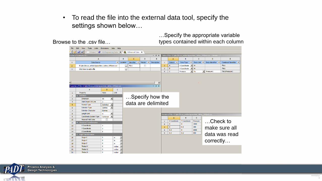
• To read the file into the external data tool, specify the
settings shown below…
Browse to the .csv file…
…Specify the appropriate variable
types contained within each column
…Specify how the
data are delimited
…Check to
make sure all
data was read
correctly…

mm/dd/yy
9
• Once you’re sure the file has been read correctly, go back
to the Project Page. Right-click on the ‘Setup’ cell of the
External Data object, and select ‘Update’.
• Once you see a green check mark indicating successful
file import, enter the Setup of the Static Structural
analysis.
…successful import!
Right-
click and
‘Update’
to import
file…

mm/dd/yy
10
• Although the file may have been successfully imported at
this stage, it still needs to get mapped (or imported) into the
Static Structural Analysis. We could have achieved this
from the Project Page by updating or refreshing the Setup
Cell of the analysis, but it can also be done from within
Mechanical by right-clicking on the ‘Imported Pressure’
object in the Tree Outline and selecting “Import Load”
…Verify the imported load by viewing
it’s contours in the graphics window
mm/dd/yy
11
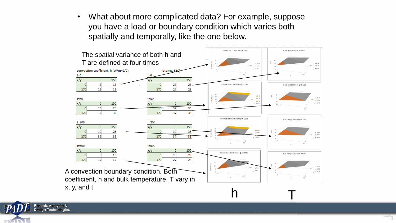
• What about more complicated data? For example, suppose
you have a load or boundary condition which varies both
spatially and temporally, like the one below.
A convection boundary condition. Both
coefficient, h and bulk temperature, T vary in
x, y, and t
h T
The spatial variance of both h and
T are defined at four times
mm/dd/yy
12
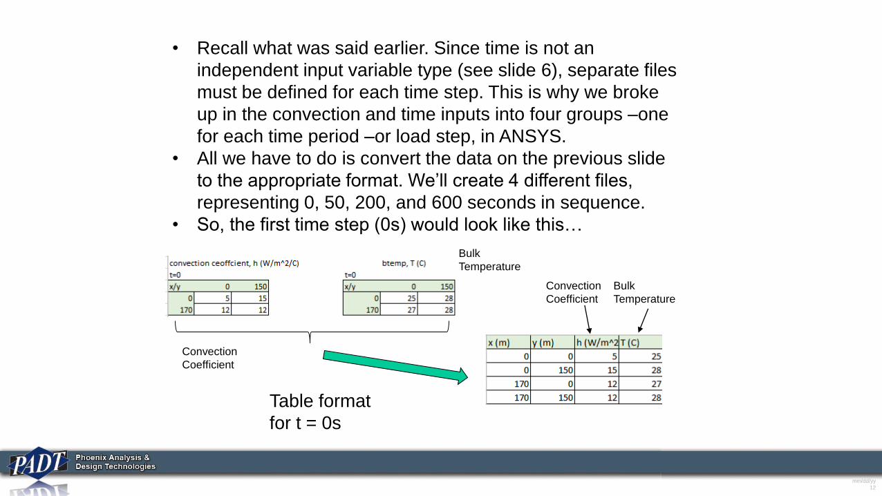
• Recall what was said earlier. Since time is not an
independent input variable type (see slide 6), separate files
must be defined for each time step. This is why we broke
up in the convection and time inputs into four groups –one
for each time period –or load step, in ANSYS.
• All we have to do is convert the data on the previous slide
to the appropriate format. We’ll create 4 different files,
representing 0, 50, 200, and 600 seconds in sequence.
• So, the first time step (0s) would look like this…
Convection
Coefficient
Bulk
Temperature
Bulk
Temperature
Convection
Coefficient
Table format
for t = 0s

mm/dd/yy
13
• Again, it is simple to save the resulting excel table in csv
(comma-delimited) format.
conv0.csv
• We simply repeat this three times, for a total of four
files –one for each of our time steps
conv50.csv
conv200.csv
conv600.csv

mm/dd/yy
14
• Next, in the Mechanical Editor, define time steps: 1s, 50s,
200s, and 600s
Define 4 times
steps under
Analysis Settings…then define the end
time for each. Note that
we chose 1s for the
first time step (because
you can’t have 0)

mm/dd/yy
15
• Then, back in the Project Page, read in the four comma-
delimited files into the external data object (which is connected
to the setup cell of a thermal transient analysis in this case)
Browse to
read in
each of
the four
files…

mm/dd/yy
16
• Specify the what’s in each column as before. Remember to
‘Start Import At’ whatever line the actual data begin (to avoid
any headers). In our case, we have to start at line 2
• Repeat this process for all files.
mm/dd/yy
17
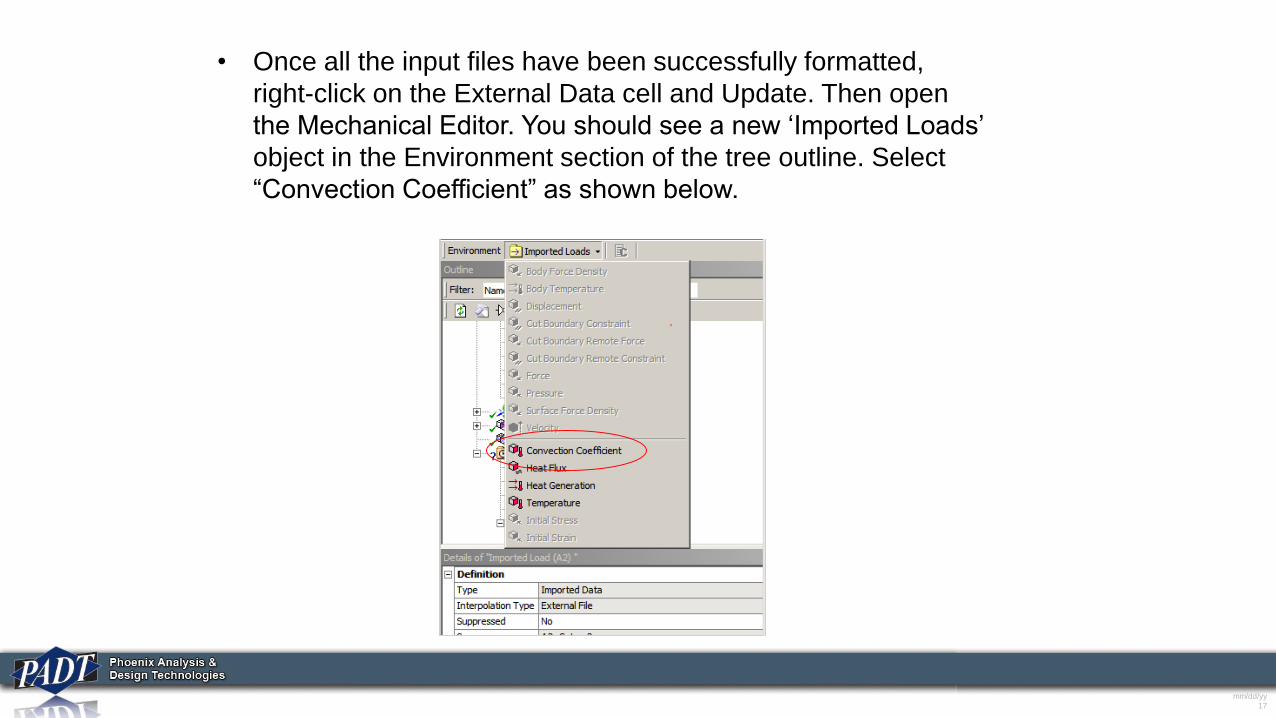
• Once all the input files have been successfully formatted,
right-click on the External Data cell and Update. Then open
the Mechanical Editor. You should see a new ‘Imported Loads’
object in the Environment section of the tree outline. Select
“Convection Coefficient” as shown below.

mm/dd/yy
18
• Select the surfaces on which to apply the load as usual
• Under ‘Imported Convection’ (in ‘Data View’), select the files that
go which each load step –specifying the end time for each.
Specify files which correspond to
each time
mm/dd/yy
19
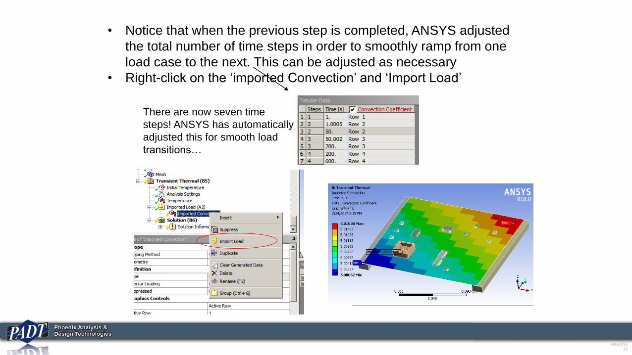
• Notice that when the previous step is completed, ANSYS adjusted
the total number of time steps in order to smoothly ramp from one
load case to the next. This can be adjusted as necessary
• Right-click on the ‘imported Convection’ and ‘Import Load’
There are now seven time
steps! ANSYS has automatically
adjusted this for smooth load
transitions…

mm/dd/yy
20
• You can view the mapped convections and bulk temperatures at
each of the import times by selecting the ‘Active Row’, and either
‘Convection Coefficient’, or ‘Temperature’ in the Details View of
the imported load.
mm/dd/yy
21
Conclusions
• The tabular loading functionality within ANSYS Mechanical offers
users the ability to vary loads spatially OR temporally. If a spatial
variation is load is required, users are restricted to only one
independent spatial variable with the options available in Mechanical
• By contrast, importing a table using the External Data tool in the
Project Schematic offers users a relatively easy and efficient means
of defining tabular loads for multiple simultaneous independent
variables.
• Another possibility (to be discussed at another time) is to modify an
existing tabular load using the Command Editor in Mechanical. In
particular, such an option could be used to overcome the
inconvenience of defining multiple files over multiple time steps.