Multi-column Deep Neural Networks for Image Classification

Dan Ciresan, Ueli Meier and Jurgen SchmidhuberIDSIA-USI-SUPSI

Galleria 2, 6928 Manno-Lugano, Switzerland{dan,ueli,juergen}@idsia.ch

Abstract

Traditional methods of computer vision and machinelearning cannot match human performance on tasks suchas the recognition of handwritten digits or traffic signs. Ourbiologically plausible, wide and deep artificial neural net-work architectures can. Small (often minimal) receptivefields of convolutional winner-take-all neurons yield largenetwork depth, resulting in roughly as many sparsely con-nected neural layers as found in mammals between retinaand visual cortex. Only winner neurons are trained. Sev-eral deep neural columns become experts on inputs pre-processed in different ways; their predictions are averaged.Graphics cards allow for fast training. On the very com-petitive MNIST handwriting benchmark, our method is thefirst to achieve near-human performance. On a traffic signrecognition benchmark it outperforms humans by a factorof two. We also improve the state-of-the-art on a plethoraof common image classification benchmarks.

1. IntroductionRecent publications suggest that unsupervised pre-

training of deep, hierarchical neural networks improves su-pervised pattern classification [2, 10]. Here we train suchnets by simple online back-propagation, setting new, greatlyimproved records on MNIST [19], Latin letters [13], Chi-nese characters [22], traffic signs [33], NORB (jittered, clut-tered) [20] and CIFAR10 [17] benchmarks.

We focus on deep convolutional neural networks (DNN),introduced by [11], improved by [19], refined and simpli-fied by [1, 32, 7]. Lately, DNN proved their mettle on datasets ranging from handwritten digits (MNIST) [5, 7], hand-written characters [6] to 3D toys (NORB) and faces [34].DNNs fully unfold their potential when they are wide (manymaps per layer) and deep (many layers) [7]. But trainingthem requires weeks, months, even years on CPUs. Highdata transfer latency prevents multi-threading and multi-CPU code from saving the situation. In recent years, how-ever, fast parallel neural net code for graphics cards (GPUs)

has overcome this problem. Carefully designed GPU codefor image classification can be up to two orders of magni-tude faster than its CPU counterpart [35, 34]. Hence, to trainhuge DNN in hours or days, we implement them on GPU,building upon the work of [5, 7]. The training algorithmis fully online, i.e. weight updates occur after each errorback-propagation step. We will show that properly trainedwide and deep DNNs can outperform all previous methods,and demonstrate that unsupervised initialization/pretrainingis not necessary (although we don’t deny that it might helpsometimes, especially for datasets with few samples perclass). We also show how combining several DNN columnsinto a Multi-column DNN (MCDNN) further decreases theerror rate by 30-40%.

2. Architecture

The initially random weights of the DNN are iterativelytrained to minimize the classification error on a set of la-beled training images; generalization performance is thentested on a separate set of test images. Our architecture doesthis by combining several techniques in a novel way:

(1) Unlike the small NN used in many applications,which were either shallow [32] or had few maps per layer(LeNet7, [20]), ours are deep and have hundreds of mapsper layer, inspired by the Neocognitron [11], with many(6-10) layers of non-linear neurons stacked on top of eachother, comparable to the number of layers found betweenretina and visual cortex of macaque monkeys [3].

(2) It was shown [14] that such multi-layered DNN arehard to train by standard gradient descent [36, 18, 28], themethod of choice from a mathematical/algorithmic pointof view. Today’s computers, however, are fast enough forthis, more than 60000 times faster than those of the early90s1. Carefully designed code for massively parallel graph-ics processing units (GPUs normally used for video games)allows for gaining an additional speedup factor of 50-100over serial code for standard computers. Given enough la-beled data, our networks do not need additional heuristics

11991 486DX-33 MHz, 2011 i7-990X 3.46 GHz

1

such as unsupervised pre-training [29, 24, 2, 10] or care-fully prewired synapses [27, 31].

(3) The DNN of this paper (Fig. 1a) have 2-dimensionallayers of winner-take-all neurons with overlapping recep-tive fields whose weights are shared [19, 1, 32, 7]. Givensome input pattern, a simple max pooling technique [27]determines winning neurons by partitioning layers intoquadratic regions of local inhibition, selecting the most ac-tive neuron of each region. The winners of some layer rep-resent a smaller, down-sampled layer with lower resolution,feeding the next layer in the hierarchy. The approach isinspired by Hubel and Wiesel’s seminal work on the cat’sprimary visual cortex [37], which identified orientation-selective simple cells with overlapping local receptive fieldsand complex cells performing down-sampling-like opera-tions [15].

(4) Note that at some point down-sampling automati-cally leads to the first 1-dimensional layer. From then on,only trivial 1-dimensional winner-take-all regions are pos-sible, that is, the top part of the hierarchy becomes a stan-dard multi-layer perceptron (MLP) [36, 18, 28]. Recep-tive fields and winner-take-all regions of our DNN oftenare (near-)minimal, e.g., only 2x2 or 3x3 neurons. This re-sults in (near-)maximal depth of layers with non-trivial (2-dimensional) winner-take-all regions. In fact, insisting onminimal 2x2 fields automatically defines the entire deep ar-chitecture, apart from the number of different convolutionalkernels per layer [19, 1, 32, 7] and the depth of the plainMLP on top.

(5) Only winner neurons are trained, that is, other neu-rons cannot forget what they learnt so far, although theymay be affected by weight changes in more peripheral lay-ers. The resulting decrease of synaptic changes per timeinterval corresponds to biologically plausible reduction ofenergy consumption. Our training algorithm is fully online,i.e. weight updates occur after each gradient computationstep.

(6) Inspired by microcolumns of neurons in the cere-bral cortex, we combine several DNN columns to form aMulti-column DNN (MCDNN). Given some input pattern,the predictions of all columns are averaged:

yiMCDNN =1

N

#columns∑j

yiDNNj(1)

where i corresponds to the ith class and j runs overall DNN. Before training, the weights (synapses) of allcolumns are randomly initialized. Various columns can betrained on the same inputs, or on inputs preprocessed indifferent ways. The latter helps to reduce both error rateand number of columns required to reach a given accuracy.The MCDNN architecture and its training and testing pro-cedures are illustrated in Figure 1.

Input

Convolution

Max Pooling

Max Pooling

Convolution

Fully connected

Fully connected

(a)

P0

DNN

DNN

P1

DNN

DNN

Pn-1

DNN

DNN

Image

AVERAGING

(b)

D

TRAINING

Image P DNN

(c)

Figure 1. (a) DNN architecture. (b) MCDNN architecture. Theinput image can be preprocessed by P0 − Pn−1 blocks. An ar-bitrary number of columns can be trained on inputs preprocessedin different ways. The final predictions are obtained by averag-ing individual predictions of each DNN. (c) Training a DNN. Thedataset is preprocessed before training, then, at the beginning ofevery epoch, the images are distorted (D block). See text for moreexplanations.

3. Experiments

We evaluate our architecture on various commonly usedobject recognition benchmarks and improve the state-of-the-art on all of them. The description of the DNN architec-ture used for the various experiments is given in the follow-ing way: 2x48x48-100C5-MP2-100C5-MP2-100C4-MP2-300N-100N-6N represents a net with 2 input images of size48x48, a convolutional layer with 100 maps and 5x5 filters,a max-pooling layer over non overlapping regions of size2x2, a convolutional layer with 100 maps and 4x4 filters,a max-pooling layer over non overlapping regions of size2x2, a fully connected layer with 300 hidden units, a fullyconnected layer with 100 hidden units and a fully connectedoutput layer with 6 neurons (one per class). We use a scaledhyperbolic tangent activation function for convolutional andfully connected layers, a linear activation function for max-pooling layers and a softmax activation function for theoutput layer. All DNN are trained using on-line gradientdescent with an annealed learning rate. During training,images are continually translated, scaled and rotated (evenelastically distorted in case of characters), whereas only theoriginal images are used for validation. Training ends oncethe validation error is zero or when the learning rate reachesits predetermined minimum. Initial weights are drawn froma uniform random distribution in the range [−0.05, 0.05].

3.1. MNIST

The original MNIST digits [19] are normalized such thatthe width or height of the bounding box equals 20 pix-els. Aspect ratios for various digits vary strongly and wetherefore create six additional datasets by normalizing digitwidth to 10, 12, 14, 16, 18, 20 pixels. This is like seeingthe data from different angles. We train five DNN columnsper normalization, resulting in a total of 35 columns forthe entire MCDNN. All 1x29x29-20C4-MP2-40C5-MP3-150N-10N DNN are trained for around 800 epochs with anannealed learning rate (i.e. initialized with 0.001 multipliedby a factor of 0.993/epoch until it reaches 0.00003). Train-ing a DNN takes almost 14 hours and after 500 trainingepochs little additional improvement is observed. Duringtraining the digits are randomly distorted before each epoch(see Fig. 2a for representative characters and their distortedversions [7]). The internal state of a single DNN is depictedin Figure 2b, where a particular digit is forward propagatedthrough a trained network and all activations together withthe network weights are plotted.

Results of all individual nets and various MCDNN aresummarized in Table 1. MCDNN of 5 nets trained withthe same preprocessor achieve better results than their con-stituent DNNs, except for original images (Tab. 1). TheMCDNN has a very low 0.23% error rate, improving stateof the art by at least 34% [5, 7, 25] (Tab. 2). This is thefirst time an artificial method comes close to the ≈0.2% er-ror rate of humans on this task [21]. Many of the wronglyclassified digits either contain broken or strange strokes, orhave wrong labels. The 23 errors (Fig. 2c) are associatedwith 20 correct second guesses.

We also trained a single DNN on all 7 datasets simul-taneously which yielded worse result (0.52%) than bothMCDNN and their individual DNN. This shows that theimprovements come from the MCDNN and not from usingmore preprocessed data.

Table 2. Results on MNIST dataset.Method Paper Error rate[%]

CNN [32] 0.40CNN [26] 0.39MLP [5] 0.35

CNN committee [6] 0.27MCDNN this 0.23

How are the MCDNN errors affected by the number ofpreprocessors? We train 5 DNNs on all 7 datasets. AMCDNN ’y out-of-7’ (y from 1 to 7) averages 5y netstrained on y datasets. Table 3 shows that more preprocess-ing results in lower MCDNN error.

We also train 5 DNN for each odd normalization, i.e.W11, W13, W15, W17 and W19. The 60-net MCDNNperforms (0.24%) similarly to the 35-net MCDNN, indicat-

(a)

L0-Input1 @ 29x29

20 @ 4x4 Filters

class "2"

L6-OutputLayer10

L5-Fully Connected

Layer150

Filters800 @ 5x5

20 @ 26x26L1-Convolutional

Layer

L2-MaxPoolingLayer

20 @ 13x13

40 @ 9x9L3-Convolutional

Layer

L4-MaxPoolingLayer

40 @ 3x3

(b)

(c)

Figure 2. (a) Handwritten digits from the training set (top row)and their distorted versions after each epoch (second to fifth row).(b) DNN architecture for MNIST. Output layer not drawn to scale;weights of fully connected layers not displayed. (c) The 23 errorsof the MCDNN, with correct label (up right) and first and secondbest predictions (down left and right).

ing that additional preprocessing does not further improverecognition.

Table 3. Average test error rate [%] of MCDNN trained on y pre-processed datasets.

y # MCDNN Average Error[%]1 7 0.33±0.072 21 0.27±0.023 35 0.27±0.024 35 0.26±0.025 21 0.25±0.016 7 0.24±0.017 1 0.23

We conclude that MCDNN outperform DNN trained onthe same data, and that different preprocessors further de-crease the error rate.

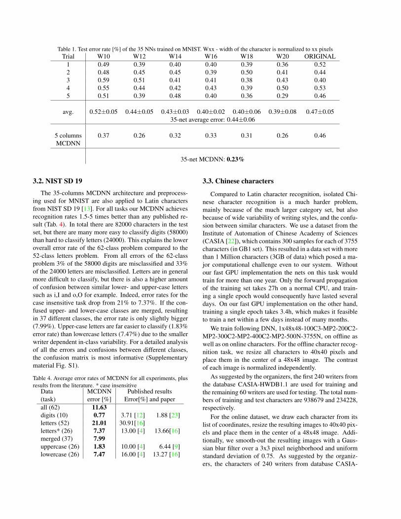
Table 1. Test error rate [%] of the 35 NNs trained on MNIST. Wxx - width of the character is normalized to xx pixelsTrial W10 W12 W14 W16 W18 W20 ORIGINAL

1 0.49 0.39 0.40 0.40 0.39 0.36 0.522 0.48 0.45 0.45 0.39 0.50 0.41 0.443 0.59 0.51 0.41 0.41 0.38 0.43 0.404 0.55 0.44 0.42 0.43 0.39 0.50 0.535 0.51 0.39 0.48 0.40 0.36 0.29 0.46

avg. 0.52±0.05 0.44±0.05 0.43±0.03 0.40±0.02 0.40±0.06 0.39±0.08 0.47±0.0535-net average error: 0.44±0.06

5 columns 0.37 0.26 0.32 0.33 0.31 0.26 0.46MCDNN

35-net MCDNN: 0.23%

3.2. NIST SD 19

The 35-columns MCDNN architecture and preprocess-ing used for MNIST are also applied to Latin charactersfrom NIST SD 19 [13]. For all tasks our MCDNN achievesrecognition rates 1.5-5 times better than any published re-sult (Tab. 4). In total there are 82000 characters in the testset, but there are many more easy to classify digits (58000)than hard to classify letters (24000). This explains the loweroverall error rate of the 62-class problem compared to the52-class letters problem. From all errors of the 62-classproblem 3% of the 58000 digits are misclassified and 33%of the 24000 letters are misclassified. Letters are in generalmore difficult to classify, but there is also a higher amountof confusion between similar lower- and upper-case letterssuch as i,I and o,O for example. Indeed, error rates for thecase insensitive task drop from 21% to 7.37%. If the con-fused upper- and lower-case classes are merged, resultingin 37 different classes, the error rate is only slightly bigger(7.99%). Upper-case letters are far easier to classify (1.83%error rate) than lowercase letters (7.47%) due to the smallerwriter dependent in-class variability. For a detailed analysisof all the errors and confusions between different classes,the confusion matrix is most informative (Supplementarymaterial Fig. S1).

Table 4. Average error rates of MCDNN for all experiments, plusresults from the literature. * case insensitive

Data MCDNN Published results(task) error [%] Error[%] and paperall (62) 11.63digits (10) 0.77 3.71 [12] 1.88 [23]letters (52) 21.01 30.91[16]letters* (26) 7.37 13.00 [4] 13.66[16]merged (37) 7.99uppercase (26) 1.83 10.00 [4] 6.44 [9]lowercase (26) 7.47 16.00 [4] 13.27 [16]

3.3. Chinese characters

Compared to Latin character recognition, isolated Chi-nese character recognition is a much harder problem,mainly because of the much larger category set, but alsobecause of wide variability of writing styles, and the confu-sion between similar characters. We use a dataset from theInstitute of Automation of Chinese Academy of Sciences(CASIA [22]), which contains 300 samples for each of 3755characters (in GB1 set). This resulted in a data set with morethan 1 Million characters (3GB of data) which posed a ma-jor computational challenge even to our system. Withoutour fast GPU implementation the nets on this task wouldtrain for more than one year. Only the forward propagationof the training set takes 27h on a normal CPU, and train-ing a single epoch would consequently have lasted severaldays. On our fast GPU implementation on the other hand,training a single epoch takes 3.4h, which makes it feasibleto train a net within a few days instead of many months.

We train following DNN, 1x48x48-100C3-MP2-200C2-MP2-300C2-MP2-400C2-MP2-500N-3755N, on offline aswell as on online characters. For the offline character recog-nition task, we resize all characters to 40x40 pixels andplace them in the center of a 48x48 image. The contrastof each image is normalized independently.

As suggested by the organizers, the first 240 writers fromthe database CASIA-HWDB1.1 are used for training andthe remaining 60 writers are used for testing. The total num-bers of training and test characters are 938679 and 234228,respectively.

For the online dataset, we draw each character from itslist of coordinates, resize the resulting images to 40x40 pix-els and place them in the center of a 48x48 image. Addi-tionally, we smooth-out the resulting images with a Gaus-sian blur filter over a 3x3 pixel neighborhood and uniformstandard deviation of 0.75. As suggested by the organiz-ers, the characters of 240 writers from database CASIA-

OLHWDB1.1 are used for training the classifier and thecharacters of the remaining 60 writers are used for testing.The resulting numbers of training and test characters are939564 and 234800, respectively.

All methods previously applied to this dataset performsome feature extraction followed by a dimensionality re-duction, whereas our method directly works on raw pixelintensities and learns the feature extraction and dimension-ality reduction in a supervised way. On the offline task weobtain an error rate of 6.5% compared to 10.01% of the bestmethod [22]. Even though much information is lost whendrawing a character from it’s coordinate sequence, we ob-tain a recognition rate of 5.61% on the online task com-pared to 7.61% of the best method [22].

We conclude that on this very hard classification prob-lem, with many classes (3755) and relatively few samplesper class (240), our fully supervised DNN beats the currentstate-of-the-art methods by a large margin.

3.4. NORB

We test a MCDNN with four columns on NORB(jittered-cluttered) [20], a collection of stereo images of3D models (Figure 3). The objects are centrally placed onrandomly chosen backgrounds, and there is also clutteringfrom a peripherally placed second object. This databaseis designed for experimenting with 3D object recognitionfrom shape. It contains images of 50 toys belonging to 5generic categories: four-legged animals, human figures, air-planes, trucks, and cars. The objects were imaged by twocameras under 6 lighting conditions, 9 elevations (30 to 70degrees every 5 degrees), and 18 azimuths (0 to 340 every20 degrees). The training set has 10 folds of 29160 imageseach for a total of 291600 images; the testing set consists oftwo folds totalizing 58320 images.

Figure 3. Twenty NORB stereo images (left image - up, right im-age - down).

No preprocessing is used for this dataset. We scale downimages from the original 108x108 to 48x48 pixels. This sizeis big enough to preserve the details present in images andsmall enough to allow fast training. We perform two roundsof experiments, using only the first two folds (to comparewith previous results that do not use the entire training data)

Table 5. Error rates, averages and standard deviations over 4 runsof a 9 layer DNN on the NORB test set.

training errors for 4 runs [%] mean[%]set size

first 4.49 4.71 4.82 4.85 4.72± 0.162 folds 4-net MCDNN error: 3.57%

all 3.32 3.18 3.73 3.36 3.40± 0.2310 folds 4-net MCDNN error: 2.70%previous state of the art: 5.00% - [8]; 5.60% - [30]

and using all training data.We tested several distortion parameters with small nets

and found that maximum rotation of 15◦, maximum transla-tion of 15% and maximum scaling of 15% are good choices,hence we use them for all NORB experiments.

To compare to previous results, we first train only on thefirst 2-folds of the data. The net architecture is deep, buthas few maps per layer: 2x48x48-50C5-MP2-50C5-MP2-50C4-MP2-300N-100N-6N. The learning rate setup is: etastart 0.001; eta factor 0.95; eta stop 0.000003. Due to smallnet size, training is fast at 156s/epoch for 114 epochs. Test-ing one sample requires 0.5ms. Even when we use less datato train, the MCDNN greatly improves the state of the artfrom 5% to 3.57% (Table 5).

Our method is fast enough to process the entire train-ing set though. We use the same architecture butdouble the number of maps when training with all10 folds: 2x48x48-100C5-MP2-100C5-MP2-100C4-MP2-300N-100N-6N. The learning rate setup remains the same.Training time increases to 34min/epoch because the net isbigger, and we use five times more data. Testing one sam-ple takes 1.3ms. All of this pays off, resulting in a very low2.70% error rate, further improving the state of the art.

Although NORB has only six classes, training and testinstances sometimes differ greatly, making classificationhard. More than 50% of the errors are due to confusionsbetween cars and trucks. Considering second predictions,too, the error rate drops from 2.70% to 0.42%, showing that84% of the errors are associated with a correct second pre-diction.

3.5. Traffic signs

Recognizing traffic signs is essential for the automotiveindustry’s efforts in the field of driver’s assistance, and formany other traffic-related applications. We use the GTSRBtraffic sign dataset [33].

The original color images contain one traffic sign each,with a border of 10% around the sign. They vary in sizefrom 15 × 15 to 250 × 250 pixels and are not necessarilysquare. The actual traffic sign is not always centered withinthe image; its bounding box is part of the annotations. Thetraining set consists of 26640 images; the test set of 12569images. We crop all images and process only within the

bounding box. Our DNN implementation requires all train-ing images to be of equal size. After visual inspection of theimage size distribution we resize all images to 48× 48 pix-els. As a consequence, scaling factors along both axes aredifferent for traffic signs with rectangular bounding boxes.Resizing forces them to have square bounding boxes.

Our MCDNN is the only artificial method to out-perform humans, who produced twice as many errors.Since traffic signs greatly vary in illumination and con-trast, standard image preprocessing methods are used toenhance/normalize them (Fig. 4a and supplementarymaterial). For each dataset five DNN are trained (ar-chitecture: 3x48x48-100C7-MP2-150C4-150MP2-250C4-250MP2-300N-43N), resulting in a MCDNN with 25columns, achieving an error rate of 0.54% on the test set.Figure 4b depicts all errors, plus ground truth and first andsecond predictions. Over 80% of the 68 errors are associ-ated with correct second predictions. Erroneously predictedclass probabilities tend to be very low—here the MCDNN isquite unsure about its classifications. In general, however,it is very confident—most of its predicted class probabili-ties are close to one or zero. Rejecting only 1% percent ofall images (confidence below 0.51) results in an even lowererror rate of 0.24%. To reach an error rate of 0.01% (a sin-gle misclassification), only 6.67% of the images have to berejected (confidence below 0.94). Our method outperformsthe second best algorithm by a factor of 3. It takes 37 hoursto train the MCDNN with 25 columns on four GPUs. Thetrained MCDNN can check 87 images per second on oneGPU (and 2175 images/s/DNN).

3.6. CIFAR 10

CIFAR10 is a set of natural color images of 32x32 pixels[17]. It contains 10 classes, each with 5000 training sam-ples and 1000 test samples. Images vary greatly within eachclass. They are not necessarily centered, may contain onlyparts of the object, and show different backgrounds. Sub-jects may vary in size by an order of magnitude (i.e., someimages show only the head of a bird, others an entire birdfrom a distance). Colors and textures of objects/animalsalso vary greatly.

Our DNN input layers have three maps, one for eachcolor channel (RGB). We use a 10-layer architecturewith very small kernels: 3x32x32-300C3-MP2-300C2-MP2-300C3-MP2-300C2-MP2-300N-100N-10N. Just likefor MNIST, the initial learning rate 0.001 decays by a fac-tor of 0.993 after every epoch. Transforming CIFAR colorimages to gray scale reduces input layer complexity but in-creases error rates. Hence we stick to the original color im-ages. As for MNIST, augmenting the training set with ran-domly (by at most 5%) translated images greatly decreasesthe error from 28% to 20% (the NN-inherent local trans-lation invariance by itself is not sufficient). By additional

(a)

(b)

Figure 4. (a) Preprocessed images, from top to bottom: original,Imadjust, Histeq, Adapthisteq, Conorm. (b) The 68 errors of theMCDNN, with correct label (left) and first and second best predic-tions (middle and right).

Table 6. Error rates, averages and standard deviations for 10 runsof a 10 layer DNN on the CIFAR10 test set. The nets in the firstrow are trained on preprocessed images (see traffic sign prepro-cessing), whereas those in the second row are trained on originalimages.

preprocessing errors for 8 runs [%] mean[%]yes 16.47 19.20 19.72 20.31 18.93± 1.69no 15.63 15.85 16.13 16.05 15.91± 0.22

8-net average error: 17.42±1.96%8-net MCDNN error: 11.21%

previous state of the art: 18.50% - [8]; 19.51% - [7]

scaling (up to ±15%), rotation (up to ±5◦), and up to ±15%translation, the individual net errors decrease by another 3%(Tab. 6). The above small maximal bounds prevent loss oftoo much information leaked beyond the 32×32 pixels rect-angle.

Figure 5. Confusion matrix for the CIFAR10 MCDNN: correctlabels on vertical axis; detected labels on horizontal axis. Squareareas are proportional to error numbers, shown both as relativepercentages of the total error number, and in absolute value. Left -images of all birds classified as planes. Right - images of all planesclassified as birds. Confusion sub-matrix for animal classes has agray background.

We repeat the experiment with different random initial-izations and compute mean and standard deviation of the er-ror, which is rather small for original images, showing thatour DNN are robust. Our MCDNN obtains a very low errorrate of 11.21%, greatly rising the bar for this benchmark.

The confusion matrix (Figure 5) shows that the MCDNNalmost perfectly separates animals from artifacts, except forplanes and birds, which seems natural, although humanseasily distinguish almost all the incorrectly classified im-ages, even if many are cluttered or contain only parts of theobjects/animals (see false positive and false negative imagesin Figure 5). There are many confusions between differentanimals; the frog class collects most false positives fromother animal classes, with very few false negatives. As ex-pected, cats are hard to tell from dogs, collectively causing15.25% of the errors. The MCDNN with 8 columns (fourtrained on original data and one trained for each preprocess-ing used also for traffic signs) reaches a low 11.21% errorrate, far better than any other algorithm.

4. ConclusionThis is the first time human-competitive results are re-

ported on widely used computer vision benchmarks. Onmany other image classification datasets our MCDNN im-proves the state-of-the-art by 30-80% (Tab. 7). We drasti-cally improve recognition rates on MNIST, NIST SD 19,Chinese characters, traffic signs, CIFAR10 and NORB. Ourmethod is fully supervised and does not use any additional

unlabeled data source. Single DNN already are sufficientto obtain new state-of-the-art results; combining them intoMCDNNs yields further dramatic performance boosts.

Table 7. Results and relative improvements on different datasets.

Dataset Best result MCDNN Relativeof others [%] [%] improv. [%]

MNIST 0.39 0.23 41NIST SD 19 see Table 4 see Table 4 30-80

HWDB1.0 on. 7.61 5.61 26HWDB1.0 off. 10.01 6.5 35

CIFAR10 18.50 11.21 39traffic signs 1.69 0.54 72

NORB 5.00 2.70 46

AcknowledgmentThis work was partially supported by a FP7-ICT-2009-6

EU Grant under Project Code 270247: A Neuro-dynamicFramework for Cognitive Robotics: Scene Representations,Behavioral Sequences, and Learning.

References[1] S. Behnke. Hierarchical Neural Networks for Image Inter-

pretation, volume 2766 of Lecture Notes in Computer Sci-ence. Springer, 2003. 1, 2

[2] Y. Bengio, P. Lamblin, D. Popovici, and H. Larochelle.Greedy layer-wise training of deep networks. In Neural In-formation Processing Systems, 2007. 1, 2

[3] N. P. Bichot, A. F. Rossi, and R. Desimone. Parallel andserial neural mechanisms for visual search in macaque areaV4. Science, 308:529–534, 2005. 1

[4] P. R. Cavalin, A. de Souza Britto Jr., F. Bortolozzi,R. Sabourin, and L. E. S. de Oliveira. An implicitsegmentation-based method for recognition of handwrittenstrings of characters. In SAC, pages 836–840, 2006. 4

[5] D. C. Ciresan, U. Meier, L. M. Gambardella, and J. Schmid-huber. Deep, big, simple neural nets for handwritten digitrecognition. Neural Computation, 22(12):3207–3220, 2010.1, 3

[6] D. C. Ciresan, U. Meier, L. M. Gambardella, and J. Schmid-huber. Convolutional neural network committees for hand-written character classification. In International Conferenceon Document Analysis and Recognition, pages 1250–1254,2011. 1, 3

[7] D. C. Ciresan, U. Meier, J. Masci, L. M. Gambardella,and J. Schmidhuber. Flexible, high performance convolu-tional neural networks for image classification. In Inter-national Joint Conference on Artificial Intelligence, pages1237–1242, 2011. 1, 2, 3, 6

[8] A. Coates and A. Y. Ng. The importance of encoding ver-sus training with sparse coding and vector quantization. InInternational Conference on Machine Learning, 2011. 5, 6

[9] E. M. Dos Santos, L. S. Oliveira, R. Sabourin, and P. Maupin.Overfitting in the selection of classifier ensembles: a compar-ative study between pso and ga. In Conference on Geneticand Evolutionary Computation, pages 1423–1424. ACM,2008. 4

[10] A. C. P.-A. M. P. V. Dumitru Erhan, Yoshua Bengio andS. Bengio. Why does unsupervised pre-training help deeplearning? Journal of Machine Learning Research, 11:625–660, 2010. 1, 2

[11] K. Fukushima. Neocognitron: A self-organizing neural net-work for a mechanism of pattern recognition unaffected byshift in position. Biological Cybernetics, 36(4):193–202,1980. 1

[12] E. Granger, P. Henniges, and R. Sabourin. Supervised Learn-ing of Fuzzy ARTMAP Neural Networks Through ParticleSwarm Optimization. Pattern Recognition, 1:27–60, 2007. 4

[13] P. J. Grother. NIST special database 19 - Handprinted formsand characters database. Technical report, National Instituteof Standards and Thechnology (NIST), 1995. 1, 4

[14] S. Hochreiter, Y. Bengio, P. Frasconi, and J. Schmidhuber.Gradient flow in recurrent nets: the difficulty of learninglong-term dependencies. In S. C. Kremer and J. F. Kolen,editors, A Field Guide to Dynamical Recurrent Neural Net-works. IEEE Press, 2001. 1

[15] D. H. Hubel and T. Wiesel. Receptive fields, binocular inter-action, and functional architecture in the cat’s visual cortex.Journal of Physiology (London), 160:106–154, 1962. 2

[16] A. L. Koerich and P. R. Kalva. Unconstrained handwrittencharacter recognition using metaclasses of characters. In Intl.Conf. on Image Processing, pages 542–545, 2005. 4

[17] A. Krizhevsky. Learning multiple layers of features fromtiny images. Master’s thesis, Computer Science Department,University of Toronto, 2009. 1, 6

[18] Y. LeCun. Une procedure d’apprentissage pour reseau a seuilasymmetrique (a learning scheme for asymmetric thresholdnetworks). In Proceedings of Cognitiva 85, pages 599–604,Paris, France, 1985. 1, 2

[19] Y. LeCun, L. Bottou, Y. Bengio, and P. Haffner. Gradient-based learning applied to document recognition. Proceed-ings of the IEEE, 86(11):2278–2324, November 1998. 1, 2,3

[20] Y. LeCun, F.-J. Huang, and L. Bottou. Learning methodsfor generic object recognition with invariance to pose andlighting. In Computer Vision and Pattern Recognition, 2004.1, 5

[21] Y. LeCun, L. D. Jackel, L. Bottou, C. Cortes, J. S. Denker,H. Drucker, I. Guyon, U. A. Muller, E. Sackinger, P. Simard,and V. Vapnik. Learning algorithms for classification: Acomparison on handwritten digit recognition. In J. H. Oh,C. Kwon, and S. Cho, editors, Neural Networks: The Statisti-cal Mechanics Perspective, pages 261–276. World Scientific,1995. 3

[22] C.-L. Liu, F. Yin, D.-H. Wang, and Q.-F. Wang. ChineseHandwriting Recognition Contest. In Chinese Conferenceon Pattern Recognition, 2010. 1, 4, 5

[23] J. Milgram, M. Cheriet, and R. Sabourin. Estimating accu-rate multi-class probabilities with support vector machines.

In Int. Joint Conf. on Neural Networks, pages 1906–1911,2005. 4

[24] M. Ranzato, Y.-L. B. Fu Jie Huang, and Y. LeCun. Unsuper-vised learning of invariant feature hierarchies with applica-tions to object recognition. In Proc. of Computer Vision andPattern Recognition Conference, 2007. 2

[25] M. Ranzato, F. Huang, Y. Boureau, and Y. LeCun. Unsu-pervised learning of invariant feature hierarchies with ap-plications to object recognition. In Proc. Computer Vi-sion and Pattern Recognition Conference (CVPR’07). IEEEPress, 2007. 3

[26] M. A. Ranzato, C. Poultney, S. Chopra, and Y. Lecun. Effi-cient learning of sparse representations with an energy-basedmodel. In Advances in Neural Information Processing Sys-tems (NIPS 2006), 2006. 3

[27] M. Riesenhuber and T. Poggio. Hierarchical models of ob-ject recognition in cortex. Nat. Neurosci., 2(11):1019–1025,1999. 2

[28] D. E. Rumelhart, G. E. Hinton, and R. J. Williams. Learn-ing internal representations by error propagation. In Paralleldistributed processing: explorations in the microstructure ofcognition, vol. 1: foundations, pages 318–362. MIT Press,Cambridge, MA, USA, 1986. 1, 2

[29] R. Salakhutdinov and G. Hinton. Learning a nonlinear em-bedding by preserving class neighborhood structure. In Proc.of the International Conference on Artificial Intelligence andStatistics, volume 11, 2007. 2

[30] D. Scherer, A. Muller, and S. Behnke. Evaluation of poolingoperations in convolutional architectures for object recogni-tion. In International Conference on Artificial Neural Net-works, 2010. 5

[31] T. Serre, L. Wolf, S. M. Bileschi, M. Riesenhuber, andT. Poggio. Robust object recognition with cortex-like mech-anisms. IEEE Trans. Pattern Anal. Mach. Intell., 29(3):411–426, 2007. 2

[32] P. Y. Simard, D. Steinkraus, and J. C. Platt. Best practices forconvolutional neural networks applied to visual documentanalysis. In Seventh International Conference on DocumentAnalysis and Recognition, pages 958–963, 2003. 1, 2, 3

[33] J. Stallkamp, M. Schlipsing, J. Salmen, and C. Igel. TheGerman Traffic Sign Recognition Benchmark: A multi-classclassification competition. In International Joint Conferenceon Neural Networks, 2011. 1, 5

[34] D. Strigl, K. Kofler, and S. Podlipnig. Performance and scal-ability of gpu-based convolutional neural networks. Paral-lel, Distributed, and Network-Based Processing, EuromicroConference on, 0:317–324, 2010. 1

[35] R. Uetz and S. Behnke. Large-scale object recognition withCUDA-accelerated hierarchical neural networks. In IEEEInternational Conference on Intelligent Computing and In-telligent Systems (ICIS), 2009. 1

[36] P. J. Werbos. Beyond Regression: New Tools for Predictionand Analysis in the Behavioral Sciences. PhD thesis, Har-vard University, 1974. 1, 2

[37] D. H. Wiesel and T. N. Hubel. Receptive fields of singleneurones in the cat’s striate cortex. J. Physiol., 148:574–591,1959. 2