multi-criteria supply chain inventory models with
TRANSCRIPT

The Pennsylvania State University
The Graduate School
The Harold and Inge Marcus Department of Industrial and Manufacturing Engineering
MULTI-CRITERIA SUPPLY CHAIN INVENTORY MODELS WITH
TRANSPORTATION COSTS
A Thesis in
Industrial Engineering
by
Ajay Natarajan
2007 Ajay Natarajan
Submitted in Partial Fulfillment of the Requirements
for the Degree of
Doctor of Philosophy
May 2007
ii
The thesis of Ajay Natarajan was reviewed and approved* by the following:
A. Ravindran Professor of Industrial Engineering Thesis Advisor Chair of Committee
Soundar R.T. Kumara Allen E. Pearce and Allen M. Pearce Professor of Industrial Engineering
Timothy W.Simpson Professor of Mechanical and Industrial Engineering
John E. Tyworth Professor of Supply Chain Management
Richard J. Koubek Professor of Industrial Engineering Head of the Department of Industrial and Manufacturing Engineering
*Signatures are on file in the Graduate School
iii
ABSTRACT
This thesis deals with developing and solving tactical inventory planning models
for a supply chain that will enable the individual companies to determine their ordering
policies efficiently under different conditions. The supply chain is modeled as a single
warehouse supplying a product to several retailers which in turn satisfies the end
consumer demand. The supply chain operates under a decentralized control, i.e., each
location is managed by an independent decision maker (DM).
In the first model, using the conventional single cost objective framework we
propose a new coordination scheme that enables the warehouse to better manage its
inventory and at the same time meet the retailers� demands without deviating too much
from their requirements. To avoid the problem of estimating marginal cost information
and to incorporate the DM�s preference information, a more realistic multiple criteria
model is then developed. To account for discounts in shipping, actual freight rate
functions are used to model transportation costs between the stages. The conflicting
criteria considered are: 1) capital invested in Inventory 2) annual number of orders 3)
annual transportation costs. While the first two models deal with deterministic demand
and constant lead time, the third model deals with stochastic demand and random lead
time. In addition to the above three criteria, fill rate is used as a fourth criterion to
measure customer satisfaction. The multiple criteria models are solved to generate several
efficient solutions. The value path method, a visual tool, is used to display tradeoffs
associated with the efficient solutions to the DM of each location in the supply chain.
The models are tested with real world data obtained from a Fortune 500 consumer
products company. Additional problems faced while extending the theoretical models to
the real world data are addressed and solved. The decision making process is simulated
by using an executive from the company to be the DM for the warehouse. The preference
information is obtained using standard multi-criteria techniques to generate the set of
efficient solutions. The DM adjudged the multi-criteria methodology to be a more
effective decision making tool since he had to evaluate tradeoffs and use his judgment to
choose the most preferred solution.
iv
TABLE OF CONTENTS
LIST OF TABLES viii
LIST OF FIGURES x
1. INTRODUCTION, MOTIVATION AND PROBLEM STATEMENT................................................................. 1
1.1. Motivation ................................................................................................................................... 2 1.2. Problem Statement ...................................................................................................................... 5
2. LITERATURE REVIEW .......................................................................................................................... 9
2.1 Overview of Supply Chain ........................................................................................................... 9 2.1.1 Supply Chain Structure.......................................................................................................... 9 2.1.2 Centralized Vs. Decentralized Supply Chains....................................................................... 10 2.1.3 Modeling Demand, Lead Time and Lead Time Demand ...................................................... 11 2.1.4 Ordering Policies ................................................................................................................. 13 2.1.5 Modeling Service Levels....................................................................................................... 14 2.1.6. Backorders Vs Lost Sales .................................................................................................... 14 2.1.7 Importance of Transportation .............................................................................................. 16
2.2. Review of Multi Criteria Optimization ..................................................................................... 18 2.2.1 General Multi-Criteria Mathematical Program.................................................................... 19 2.2.2 Terminology Associated with MCDM................................................................................... 19 2.2.3 Approaches to Solve MCMP................................................................................................. 20 2.2.4 Pλ method............................................................................................................................. 22
2.3 Literature review........................................................................................................................ 23 2.3.1 Single Location Inventory Control Models........................................................................... 24 2.3.2 Supply Chain Inventory Models ........................................................................................... 27
2.4 Contribution of the Research ..................................................................................................... 35
3. A MODIFIED BASE PERIOD POLICY FOR A SINGLE WAREHOUSE MULTI RETAILER SYSTEM.............. 39
3.1. Introduction............................................................................................................................... 39 3.1.1. Notation .............................................................................................................................. 40 3.1.2. EOQ Problem...................................................................................................................... 41 3.1.3. Economic Reorder Interval Problem ................................................................................... 41
3.2. Problem Description.................................................................................................................. 41 3.2.1. Assumptions........................................................................................................................ 42 3.2.2. Base Period Policy .............................................................................................................. 42
3.3. Modified Base Period Policy...................................................................................................... 42 3.3.1. Model Formulation ............................................................................................................. 42
v
3.3.2. Setting TB: A Different Perspective ..................................................................................... 43 3.3.3. Another Interpretation of TB ............................................................................................... 43 3.3.4. Solution to Problem (MRi) .................................................................................................. 44
3.4. Analysis of the Modified Base Period Policy............................................................................. 46 3.4.1. Grouping Retailers.............................................................................................................. 46 3.4.2. Effectiveness of the Policy................................................................................................... 47
3.5. Warehouse�s Ordering Policy ................................................................................................... 53 3.5.1. Average Inventory at the Warehouse................................................................................... 53 3.5.2. Warehouse�s Optimization Problem .................................................................................... 59 3.5.3. Solution to Problem (W)...................................................................................................... 59
3.6. Algorithm for the Modified Base Period Policy ........................................................................ 61 3.7. Final Comments on the Modified Base Period Policy............................................................... 62 3.8. Example Problem ...................................................................................................................... 63 3.9. Summary ................................................................................................................................... 66
4. DETERMINISTIC MULTI-CRITERIA MODEL FOR A SUPPLY CHAIN WITH TRANSPORTATION COSTS... 67
4.1. Introduction............................................................................................................................... 67 4.2. Problem Description.................................................................................................................. 67
4.2.1. Assumptions........................................................................................................................ 68 4.2.2. Notation .............................................................................................................................. 68
4.3. Retailer�s Model Formulation ................................................................................................... 69 4.3.1 Retailer�s Multi-Criteria Problem ........................................................................................ 74 4.3.2 Solution Procedure to Solve Problem (Ri) ............................................................................ 74 4.3.3 Modified Retailer�s Problem ................................................................................................ 77 4.3.4 Solution Procedure to Solve Problem (MRi)......................................................................... 78
4.4. Warehouse�s Model Formulation.............................................................................................. 80 4.4.1 Warehouse�s Multi-Criteria Problem ................................................................................... 82 4.4.2 Solution Procedure to Solve Problem (W) ............................................................................ 83
4.5. Algorithm .................................................................................................................................. 86 4.6. General MCMP for Retailer and Warehouse ........................................................................... 88 4.7. Example Problem ...................................................................................................................... 90 4.8. Summary ................................................................................................................................. 102
5. STOCHASTIC MULTI CRITERIA MODEL FOR A SUPPLY CHAIN WITH TRANSPORTATION COSTS ...... 103
5.1. Introduction............................................................................................................................. 103 5.2. Problem Description................................................................................................................ 103
5.2.1. Assumptions...................................................................................................................... 103 5.2.2. Notation ............................................................................................................................ 105
vi
5.3. Retailer�s Model Formulation ................................................................................................. 106 5.3.1. Retailer�s Multi-Criteria Problem...................................................................................... 110 5.3.2. Solution Procedure to Solve Problem (Ri) ......................................................................... 111
5.4. Evaluation of Lead Time Demand (LTD) Distributions ......................................................... 114 5.4.1. Case 1: Demand-Poisson Distribution, Lead Time-General Discrete Distribution ............ 115 5.4.2. Case 2: Demand-Compound Poisson Distribution, Lead Time-General Discrete Distribution
................................................................................................................................................... 117 5.4.3. Case 3: Demand-Normal Distribution, Lead Time-General Discrete Distribution............. 124
5.5. Warehouse�s Problem ............................................................................................................. 126 5.5.1. Warehouse�s Multi-Criteria Problem ................................................................................ 131 5.5.2. Solution Procedure to Solve Problem (W) ......................................................................... 131
5.6. Backorder Assumption............................................................................................................ 134 5.6.1. Retailer ............................................................................................................................. 134 5.6.2. Warehouse ........................................................................................................................ 134
5.7. Example Problem .................................................................................................................... 136 5.8 Summary .................................................................................................................................. 148
6 CASE STUDY ..................................................................................................................................... 149
6.1 Introduction.............................................................................................................................. 149 6.2 Case Study Description ............................................................................................................ 149 6.3 Case Study 1: Chapter 3........................................................................................................... 149
6.3.1 Overview ............................................................................................................................ 149 6.3.2 Results ............................................................................................................................... 150 6.3.3 Difficulties Encountered .................................................................................................... 152
6.4 Case Study 2: Chapter 4........................................................................................................... 153 6.4.1 Overview ............................................................................................................................ 153 6.4.2 Results ............................................................................................................................... 154 6.4.3 Difficulties Encountered .................................................................................................... 159
6.5 Case Study 3: Chapter 5........................................................................................................... 162 6.5.1 Overview ............................................................................................................................ 162 6.5.2 Results ............................................................................................................................... 164
6.6 Summary .................................................................................................................................. 167
7 CONCLUSIONS AND FUTURE WORK .................................................................................................. 168
7.1 Overview................................................................................................................................... 168 7.2 Conclusions............................................................................................................................... 169
7.3 Managerial Implications .......................................................................................................... 171
vii
7.4 Limitations................................................................................................................................ 172 7.5 Future Work............................................................................................................................. 172
BIBLIOGRAPHY .................................................................................................................................... 174
viii
LIST OF TABLES
Table 2.1 Joint Distribution of LTD�����������������...���������12
Table 2.2 Contribution of Chapter 3��������������������������...35
Table 2.3 Contribution of Chapter 4��������������������������...36
Table 2.4 Contribution of Chapter 5��������������������������...37
Table 3.1 Worst Case Deviation Bounds for n≥2 Case �������������������.49
Table 3.2 Data for Example Problem.������������..�������������..63
Table 3.3 Output of Problem (Ri)����������������������������64
Table 3.4 Output of Problem (MRi)���������������������������65
Table 4.1 Data for Example Problem..�������.������������������..91
Table 4.2 Freight Rate Data������������������������������.91
Table 4.3 Freight Rate Data with Indifference Points�������������������...91
Table 4.4 Summary of Curve Fitting��������������������������..92
Table 4.5 Bounds on Order Quantity��������������������������.93
Table 4.6 Criteria Values for the Retailers�...����..�����������������...95
Table 4.7 Normalized Criteria Values for the Retailers �������������...����...95
Table 4.8 Most Preferred Solution for the Retailers..�������������������...98
Table 4.9 Summary of Results for the Retailers ���������������������...98
Table 4.10 Efficient Solutions for the Warehouse ��������...�����������...100
Table 4.11 Criteria and Normalized Criteria Values for the Warehouse�����������.101
Table 5.1 Demand Distribution for Retailer ����������������������...136
Table 5.2 Lead Time Distribution for Retailer ������.��������������......137
Table 5.3 Bounds on Decision Variables����������������������...........137
Table 5.4 Weight Combinations����������������������........................138
Table 5.5 Sample Calculations����������������������...........................139
Table 5.6 Criteria Values for the Retailers�...����.. ��������...��������.140
Table 5.7 Normalized Criteria Values for the Retailers �������������...����.140
Table 5.8 Ordering Policy of the Retailers������.. ������������.����...144
Table 5.9 Most Preferred Criteria Values for the Retailers..����������...�����..144
Table 5.10 Distribution of Lead Time at the Warehouse..����.����..��������...145
Table 5.11 Efficient Solutions for the Warehouse ��������...�����������...146
Table 5.12 Criteria and Normalized Criteria Values for the Warehouse����.�������146
Table 6.1 Output of EOQ Problem for Retailers���������������������.150
Table 6.2 Output of Modified Problem for Retailers�������������������..151
Table 6.3 Output of Modified Problem for Retailers in Tier II������������...��..153
Table 6.4 Comparison of Results with and without Tier Approach �������������.153
ix
Table 6.5 Output of Problem (Ri)���������������������������..155
Table 6.6 Output of Modified Problem for Retailers�������������������..156
Table 6.7 Weights Using Method 1���.����..�������������������157
Table 6.8 Weights Using Method 2���.����..�������������������157
Table 6.9 Strength of Preferences���������������������������.158
Table 6.10 Weights Using Method 3���.�����..�����������������..158
Table 6.11 Efficient Solutions for the Warehouse ��������...�����������...159
Table 6.12 Output of Modified Problem for Retailers in Tier II������������...��160
Table 6.13 Output of the Warehouse�s Problem Including Tier I Retailers����������.160
Table 6.14 Output of the Warehouse�s Problem Including Tier II Retailers���������...161
Table 6.15 Normality Test for Demand ���������...����������....................163
Table 6.16 Distribution of Lead Time...�������������������........................164
Table 6.17 Ordering Policy of the Retailers ��������������������............164
Table 6.18 Criteria Values for the Retailers�...����.. ��������...�������...165
Table 6.19 Weights Using Method 1��������...�����������������..166
Table 6.20 Weights Using Method 2��������...�����������������..166
Table 6.21 Strength of Preferences�....������������������������...166
Table 6.22 Weights Using Method 3��������..������������.�����..166
Table 6.23 Efficient Solutions for the Warehouse ��������..��.���������...167

x
LIST OF FIGURES
Figure 1.1 Logistics Cost as a Percent of GDP�����������������������.2
Figure 1.2 Components of the Logistics Cost�����������������������...3
Figure 1.3 Supply Chain System under Consideration...�������������������5
Figure 2.1 Supply Chain Network����������������������������.9
Figure 2.2 Arborescence Structure���������������������������.10
Figure 2.3 Serial Supply Chain�.. ���������������������������.10
Figure 2.4 Supported and Unsupported Efficient Points�������.�����������.23
Figure 2.5 Classification of Literature Review����������������������..23
Figure 3.1 Worst Case Deviation Variation�����������������������...50
Figure 3.2 Worst Case Deviation within a Cluster��������������������....51
Figure 3.3 *B TT Vs. Deviation for n=1 Case������...�.��������������...53
Figure 3.4 Inventory Pattern of the Retailers��������������������............54
Figure 3.5 Inventory Pattern of the Warehouse��������������������........56
Figure 3.6 Flow Chart of the Modified Base Period Policy�����������������..62
Figure 4.1 Retailers Inventory Pattern ��������������������......................69
Figure 4.2 Freight Rate Function ����������..���������.................................72
Figure 4.3 Value Path Graphs for Retailers ���������...����������...............97
Figure 4.4 Value Path Graph for Warehouse ���������...����������..........101
Figure 5.1 Retailers Inventory Pattern ��������������������....................107
Figure 5.2 Value Path Graphs for Retailers ���������...����������.............142
Figure 5.3 a and b Behavior of Fill Rate/Cycle Service Level��������������.�...143
Figure 5.4 Value Path Graph for Warehouse ���������...����������..........147

1
Chapter 1
INTRODUCTION, MOTIVATION AND PROBLEM STATEMENT
Over the past decade and a half there has been an increasing number of articles in
the field of multi-echelon systems, popularly called supply chain management. The
reason for the continuing fascination in this area among researchers is not only due to the
complexity that arises from the interactions among the various stages/echelons but also
due to the enormous practical applications in the real world.
A comprehensive definition of a supply chain given by Min and Zhou (2002) is as
follows: the supply chain can be defined as an integrated system or network which
synchronizes a series of inter-related business processes in order to:
• Acquire raw materials.
• Add value to raw materials by transforming them into finished/semi-finished
goods.
• Distribute these products to distribution centers or sell to retailers or directly to
the customers.
• Facilitate the flow of raw materials/finished goods, cash and information among
the various partners which include suppliers, manufacturers, retailers, distributors
and third-party logistic providers (3PL).
Thus the main objective of the supply chain is to maximize the profitability of not
just a single firm but also all of the partners involved. This can only be done if all the
partners in the supply chain think �Win-Win� and are not concerned about optimizing
their individual performance. The major drivers of the supply chain are (Chopra and
Meindl, 2001):
• Inventory.
• Transportation.
• Facilities.
• Information.
From an optimization perspective, the main focus in the area of multi-echelon
systems has been the problem of inventory management. The inventory problem consists
of answering the two fundamental questions: 1. When to order? and 2. How much to

2
order? These two questions are conflicting in the sense that, if we decide to order
frequently, then we order in lesser quantities, and similarly, if we decide to order less
frequently, then we order larger quantities. Thus, within each company there are
conflicting objectives. Hence, appropriate tradeoffs have to be made within each
company for the inventory function alone.
Within each company, there exist inter-functional tradeoffs. For example, the
tradeoff between the inventory function and the transportation function has been well
studied for problems involving single stocking points (Baumol and Vinod, 1970, Das,
1974, Buffa and Reynolds, 1977, Constable and Whybark, 1978). A faster and more
reliable transportation mode can be used to ship smaller batches more frequently leading
to a reduction in the amount of inventory stored at the stocking point while maintaining
the same service level, but the decision maker (DM) has to make sure that the increase in
transportation costs is offset by reduction in inventory costs. Capturing such tradeoffs
within each company for all the companies in a multi-echelon system is a challenging
problem.
1.1 Motivation
To give an idea about how significant the inventory and transportation costs are,
Fig. 1.1 (Cook, 2006) tracks the total logistics cost as a percent of the Gross Domestic
Product (GDP) of U.S. over the past decade. The logistics cost includes cost of inventory,
transportation and logistics administration.
Fig. 1.1: Logistics Cost as a Percent of GDP

3
The total logistics decreased from the mid nineties to 2003 mainly due to the
reduction in inventory holding costs due to the Just in time (JIT) initiatives undertaken by
the U.S. companies. Since 2003, the logistics costs have been increasing. This is due to
the increase in inventory holding and transportation costs. Inventory holding costs
increased due to higher interest rates, and the companies stocking up their warehouses to
prevent disruptions in their supply after the 9/11 terrorist attacks, while transportation
costs increased due to inflating gas prices and high labor turnover (Cook, 2006).
In 2005 the logistics cost as a percent of the GDP was 9.5% and was valued at
$1.183 trillion. The amount spent on each component of the logistics cost is shown in
Fig. 1.2 (Cook, 2006).
0
100
200
300
400
500
600
700
800
Cos
t (B
illio
n)
Inventory Carrying CostsTransportation CostsAdministration Costs
Fig. 1.2: Components of the Logistics Cost
The inventory carrying cost was estimated to be $393 billion, considerably less
than the transportation cost, which was estimated to be $744 billion. The transportation
cost accounted for nearly 6% of the GDP. Out of the $744 billion, $583 billion was spent
on transportation using trucks reiterating the fact that road mode is still the preferred
method for transportation in the U.S.

4
There has been an increase of about $61 billion dollar in the inventory costs from
the year 2004. According to Cook (2006) a bigger concern is the increase in the road
transportation costs of about $74 billion dollars from 2004. The road transportation costs
are expected to go up over the coming years due to increasing freight rates, aging
infrastructure and improving security measures.
From the preceding paragraphs, it is clear that inventory and transportation
management are crucial to reducing costs in the supply chain. The decision maker (DM)
of a company has to pay careful attention while determining the ordering policy (when to
order and how much to order) so as to take advantage of the freight rate discount and at
the same time not stock too much while providing the necessary service to its customers.
Thus, the DM has to balance several conflicting criteria before choosing the most
preferred solution.
Inventory decisions made without taking into account transportation costs would
fail to take advantage of the economies of scale in shipping. The first paper to address
this issue was due to Baumol and Vinod (1970). Since then a lot of work has been done
in determining inventory policies when transportation costs are included (Das, 1974,
Buffa and Reynolds, 1977, Constable and Whybark, 1978, Lee, 1986, Tyworth and Zeng,
1998, etc.). Researchers who have incorporated transportation costs in supply chain
inventory models include Ganeshan (1999), Qu et al. (1999), Chan et al. (2002), Toptal et
al. (2003), etc.
With the imminent rise in transportation costs, each company in the supply chain
should pay close attention to its logistics function. Cartin and Ferrin (1996) list some of
the advantages to companies that manage their inbound logistics. This is discussed in
more detail in Chapter 2.
The conventional way of determining ordering policies for a single location have
been by optimizing a single cost objective (Hadley and Whitin, 1963). Other researchers
like Brown (1961), Starr and Miller (1962), Gardner and Dannenbring (1979) and Agrell
(1995) argue that marginal costs information such as ordering costs, inventory holding
costs, cost of lost sales/backorders, etc. are difficult to estimate. A multi-criteria
approach obviates this problem as the marginal cost information is not needed. Most
multi-echelon inventory models also use a single cost objective (Sherbrooke, 1968,

5
Schwarz, 1973, Deuermeyer and Schwarz, 1981, Roundy, 1985, Axsater, 1990a, etc.).
Bookbinder and Chen (1992), Thirumalai (2001) and DiFillipo (2003) have modeled the
supply chain as a multi-criteria problem.
Since the DM is an integral part of any system, his/her preference information
must be incorporated during the decision making process. This aspect is completely
ignored by the single objective methods. Single objective optimization gives the DM an
optimal solution (if it exists) or a �good� solution based on some heuristic procedure, but
in a multi-criteria approach the DM is provided with several efficient solutions. An
efficient solution is defined as one in which any further improvement of a criterion would
result in the worsening of at least one other criterion. The DM after evaluating tradeoffs
among the conflicting criteria will then be able to choose the most preferred solution.
1.2 Problem Statement
The problem setting consists of a manufacturer supplying a single product to a
warehouse (owned by the manufacturer) which in turn distributes the product to multiple
retailers in order to meet the end customer demand as shown in Fig. 1.3. The
manufacturer is assumed to have infinite capacity. The goal is to determine the ordering
policies for each retailer and the warehouse efficiently under different scenarios.
Fig. 1.3: Supply Chain System under Consideration
This system operates in a decentralized framework, i.e., there are decision makers
at each location trying to optimize their own objectives. The individual retailer problems

6
are solved, and the output of the retailer problem is used as input to solve the warehouse
problem.
The transportation cost has two components, namely, the inbound transportation
cost at the warehouse and the inbound transportation cost at each of the retailers. The
inbound transportation cost at the warehouse is modeled using full truck load (TL) freight
rates since a single supplier is supplying to the warehouse. The inbound transportation
cost at each retailer is modeled using less than full truck load (LTL) freight rates, since
the order quantity will be smaller. Continuous functions are used to model the
transportation cost based on how well they fit the freight rate data.
Each location in the supply chain is assumed to follow a continuous review policy.
A continuous review policy is one in which the decision maker places an order when on
hand inventory depletes to a reorder point. Giant retailers (e.g., Walmart) use Electronic
Data Interchange (EDI) to place an order to their suppliers as soon as the reorder point is
reached. The inventory level is tracked using bar codes.
The external demand can be either deterministic or stochastic. We consider both
cases in this thesis. The time taken by the preceding stage to replenish an order called the
lead time can be instantaneous, deterministic or stochastic. If the demand and lead time
are deterministic, then the new order arrives exactly when the on hand inventory reaches
zero. But this is not the case when either demand or lead time or both are random
variables. In such a scenario, there is a possibility that when the new order arrives the
location has some inventory or is already out of stock. The latter leads to a stockout
condition. In a stockout situation, excess demand can either be backordered or lost. The
DM of a company has to carefully balance the amount of inventory maintained at its shelf
so as to not have excess inventory and at the same time reduce stockout situations as it
would lead to customer dissatisfaction
Chapter 2 starts of with a brief review of some of the important aspects that must
be considered in modeling inventory and transportation components in a supply chain.
Then, the important concepts in multi-criteria optimization and a review of some of the
methods that are used to solve these problems are discussed. This is followed by a
detailed literature review pertaining to single location and supply chain inventory models.
Chapter 2 concludes with the contributions of the research.
7
In Chapter 3, a new control policy is proposed that enables the warehouse to
better manage its inventory and at the same time meet the retailers� demands without
deviating too much from their requirements. The retailers face deterministic demand.
Instantaneous replenishment is assumed at the retailers and the warehouse. Assuming the
availability of marginal cost information such as inventory holding and ordering costs, a
single objective cost model is developed for each location. Closed-form expressions are
derived which facilitates determining the ordering policies efficiently. Using the structure
of the solution, a theoretical method is developed to group retailers into clusters based on
their importance to the warehouse. The effectiveness of the policy is tested by developing
theoretical bounds on the deviation from the optimal solution of the retailers.
In Chapter 4, the single cost objective model of Chapter 3 is extended to the case
where marginal cost information is not known. We model the supply chain problem as a
multi-criteria problem with three criteria: 1) capital invested in inventory 2) annual
number of orders placed and 3) annual transportation costs. Lead times are assumed to be
deterministic. Transportation costs are considered between each stage and are modeled
using appropriate continuous functions. Efficient solutions are generated by changing the
weight assigned to each criterion. A graphical tool is used to visualize the tradeoff
information which would enable the DM of each location to choose the most preferred
solution.
Chapter 5 extends the deterministic multi-criteria model with transportation costs
to the case where both demands and lead times are random variables. The demands faced
by the retailers are independent, non-identical Poisson random variables. The case of
compound Poisson demand and normal demands are also considered. The lead times are
assumed to follow any discrete distribution. The demand at the warehouse is
approximated by a normal distribution using renewal theory concepts. Excess demand at
the retailers and the warehouse is assumed to be lost. We also discuss how the backorders
case can be handled. Fill rate is the fourth criterion and is used to measure customer
satisfaction. Fill rate is defined as the proportion of demand met from on-hand inventory.
The solution procedure used to solve the multi-criteria model is similar to the one in
Chapter 4.
8
In Chapter 6, we apply the methodologies developed in Chapters 3, 4 and 5 using
real world data obtained from a Fortune 500 consumer products company. Some of the
problems faced while extending the theoretical models to the real world data are
addressed. A tool is created using Excel and Visual Basic (VB) macros to automate
certain aspects of the solution methodologies. We used an executive from the Fortune
500 Company to be the DM at the warehouse to analyze the various tradeoffs and hence,
choose the most preferred solution.
Chapter 7 discusses the conclusions and future work.

9
Chapter 2
LITERATURE REVIEW
2.1 Overview of Supply Chain
This section provides a brief introduction to some basic terminologies and
concepts of supply chains. Also, an overview of modeling the parameters that are needed
in the latter chapters is given.
2.1.1 Supply Chain Structure
The most general supply chain structure is called the supply chain network where
there are many companies in each stage, and each company in a particular stage is
supplied by one or more companies in the preceding stage, and similarly each company
can supply to one or more companies in the succeeding stage. Such a structure is very
hard to analyze as the number of possible interactions within each stage is very large. A
possible scenario of a supply chain network is depicted in Fig. 2.1.
Fig. 2.1: Supply Chain Network
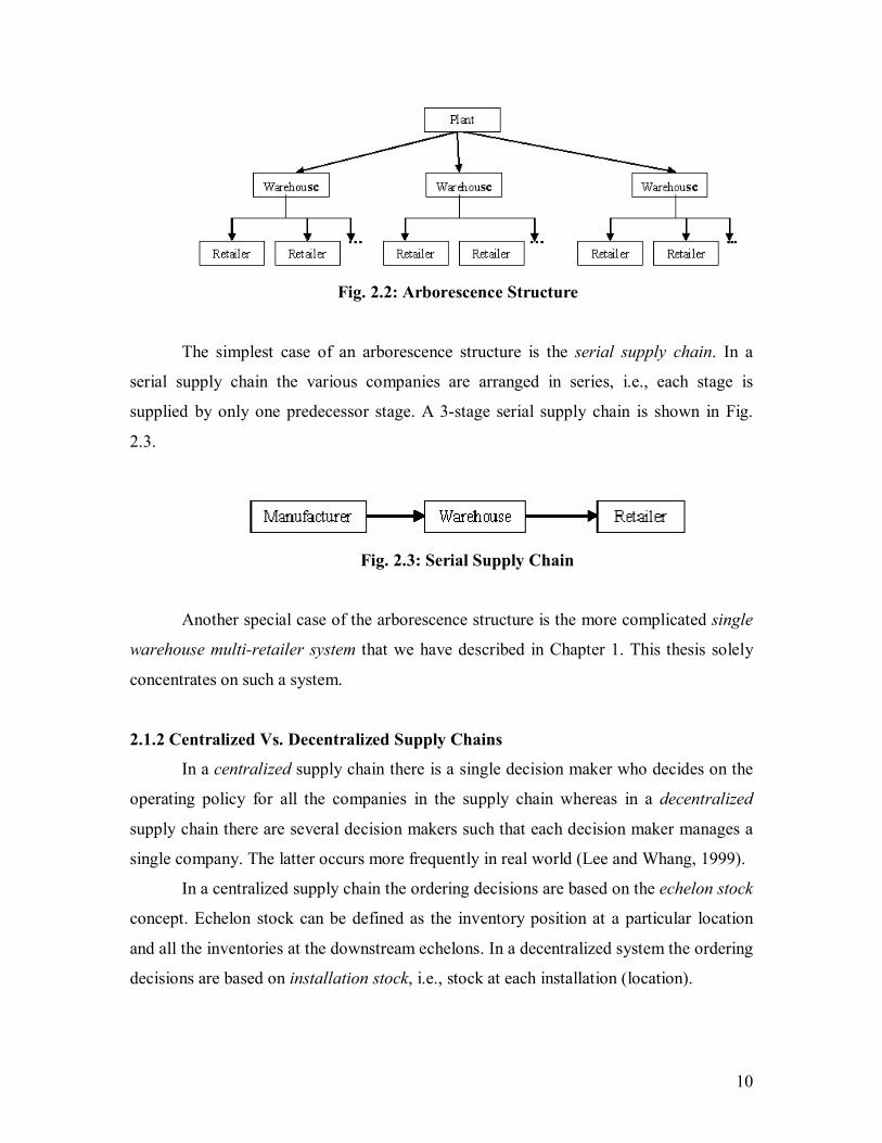
Hence, most of the research done in this area has been restricted to arborescence
structures (see Fig. 2.2). In such structures, a company in a particular stage can be
supplied by at most one predecessor but it can supply to at least one company in the
succeeding stage.
10
Fig. 2.2: Arborescence Structure
The simplest case of an arborescence structure is the serial supply chain. In a
serial supply chain the various companies are arranged in series, i.e., each stage is
supplied by only one predecessor stage. A 3-stage serial supply chain is shown in Fig.
2.3.
Fig. 2.3: Serial Supply Chain
Another special case of the arborescence structure is the more complicated single
warehouse multi-retailer system that we have described in Chapter 1. This thesis solely
concentrates on such a system.
2.1.2 Centralized Vs. Decentralized Supply Chains
In a centralized supply chain there is a single decision maker who decides on the
operating policy for all the companies in the supply chain whereas in a decentralized
supply chain there are several decision makers such that each decision maker manages a
single company. The latter occurs more frequently in real world (Lee and Whang, 1999).
In a centralized supply chain the ordering decisions are based on the echelon stock
concept. Echelon stock can be defined as the inventory position at a particular location
and all the inventories at the downstream echelons. In a decentralized system the ordering
decisions are based on installation stock, i.e., stock at each installation (location).
11
An immediate research question is the comparison of centralized and
decentralized systems. Intuitively a centralized control should dominate the decentralized
control as in the centralized case decisions are made by optimizing all the objectives of
the entire supply chain, while in a decentralized system each location is going to make its
own independent decisions, which might be best for them, but might not be good for the
supply chain.
Axsater and Rosling (1993) showed that a centralized control dominates a
decentralized control for N-stage serial supply chain where each location in the system
follow a (Q,r) policy. The results were extended to a general assembly system.
Axsater and Juntti (1996) determined the worst-case performance of installation
stock policy when compared to echelon stock policy results for the case of a 2-stage
serial supply chain under a deterministic scenario. For stochastic demand, a simulation
was performed and the results indicated that a centralized control dominated a
decentralized control when the warehouse lead times are long and vice-versa when the
warehouse lead times are short.
DiFillipo (2003) showed through examples that the above intuitive result does not
hold when transportation costs are included in the model.
2.1.3 Modeling Demand, Lead Time and Lead Time Demand
2.1.3.1 Demand
Demand of a particular product can be deterministic or probabilistic. In the
deterministic case it is possible to determine the state of the system at any given point in
time. However, the same cannot be said in the probabilistic case since the demand is a
random variable. The demand in such cases is assumed to have a known probability mass
function (pmf) in the discrete case or a probability density function (pdf) in the
continuous case. Since most companies keep track of historical data, forecasting
techniques can be used to determine the distribution of future demand (Starr and Miller,
1962).
12
2.1.3.2 Lead Time
The lead time is the time between when an order is placed and when it is received
at the customer end. It comprises mainly the ordering time and transit time. The ordering
time includes preparing and processing the order. Transit time is the time spent by the
goods in a particular transportation mode. We assume that the lead time equals transit
time. Some researchers have emphasized including ordering time by treating it as a
constant in addition to the transit time, e.g., Tyworth and Zeng (1998) and Ganeshan
(1999). Including the constant ordering time poses no problem and is addressed as an
extension to the basic model in Chapter 5.
Based on the lead time between two locations, inventory models can be classified
as instantaneous replenishment (zero lead time), constant lead time and stochastic lead
time (Ravindran, 2002). The first case simplifies the analysis a great deal. The second
case is very similar to the first except that it is a more realistic approach. The third case
represents real life situations where deliveries at a particular stocking point arrive late due
to randomness in the lead time.
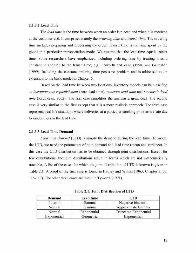
2.1.3.3 Lead Time Demand
Lead time demand (LTD) is simply the demand during the lead time. To model
the LTD, we need the parameters of both demand and lead time (mean and variance). In
this case the LTD distribution has to be obtained through joint distributions. Except for
few distributions, the joint distributions result in forms which are not mathematically
tractable. A list of the cases for which the joint distribution of LTD is known is given in
Table 2.1. A proof of the first case is found in Hadley and Whitin (1963, Chapter 3, pp.
116-117). The other three cases are listed in Tyworth (1991).
Table 2.1: Joint Distribution of LTD
Demand Lead time LTD Poisson Gamma Negative binomial Normal Gamma Approximate Gamma Normal Exponential Truncated Exponential
Exponential Geometric Exponential
13
The standard way of avoiding this issue (determining joint distributions) was to
assume that the LTD is normally distributed with mean and variance given by:
LDLD µµ=µ (2.1)
2L
2D
2DL
2LD σµ+σµ=σ (2.2)
where:
Dµ - Mean period demand
Dσ - Standard deviation of period demand
Lµ - Mean lead time
Lσ - Standard deviation of lead time
Eppen and Martin (1988) and Tyworth (1991) state that this approach for characterizing
the LTD as a normal distribution can lead to inaccurate estimates of safety stock.
Eppen and Martin (1988) and Tyworth (1992) suggest the use of a convex
combination approach for modeling the LTD. Provided that the demands are independent
between time periods, the LTD distribution can be modeled as a weighted sum of the
conditional demand distributions over the range of the lead time values. Tyworth and
Zeng (1998) state that this approach can be used for period demands that follow Normal,
Poisson, Gamma and Exponential distributions and lead times having general discrete
distribution or discrete approximations of continuous probability distributions. For
example, if demand is normally distributed, ( )2DD ,N σµ and the lead time takes on
discrete values j = 1,..,n with probability pj, then the conditional LTD ~ ( )2DD j,jN σµ .
We use this result in Chapter 5, which deals with determining ordering policies under
both stochastic demand and lead time. We also prove that the convex combination
approach can be used for a special case of a compound Poisson distribution called the
geometric Poisson distribution.
2.1.4 Ordering Policies
Inventory models, depending on the ordering policy followed by a location can be
classified as continuous review or period review. In a continuous review policy a location
places an order of Q units when a reorder point of r units is reached. For this reason it is
also called a (Q,r) policy. The time between orders in this case is a random variable. In a

14
periodic review policy a location places an order every T periods to raise the inventory
level up to S units. For this reason a periodic review policy is also called a (T,S) policy.
Here, the order quantity is a random variable.
A more general policy is the (S,s) policy wherein the location orders up to S units
when the reorder point is less than or equal to s units. An (S,s) policy can be either
continuously reviewed or periodically reviewed.
2.1.5 Modeling Service Levels
When the demand or lead time or both are random variables, LTD is also a
random variable. As a result, the on-hand inventory when an order arrives is not known
with certainty. When the LTD exceeds the reorder point, stock-outs occur. One obvious
way of preventing stock-outs is to increase the product availability, but increasing the
product availability increases the safety stock and thus the inventory holding cost. Hence,
there should be a tradeoff between availability and cost.
In case of a stockout, one of the two things can happen: 1) excess demand is
backordered or 2) excess demand is lost. In either case, we have to determine a stockout
cost. In practice, stock-out cost is very hard to quantify as it consists of loss of goodwill
with customers, downstream echelon retard, etc. An implicit way to avoid estimating
stockout costs is for the DM to specify a target service level and make sure it is met by
adding it as a constraint to the optimization problem.
There are two types of service level objectives:
1. Cycle service level (CSL): This is the fraction of order cycles in which all the
customer demand is met.
2. Fill rate (FR): This is the proportion of demand that is filled from existing
inventory.
2.1.6. Backorders Vs Lost Sales
Before we distinguish between the backorders and lost sales case, the following
terms are defined:
• On-hand Inventory: The inventory that is available on the shelf.
• Net Inventory: On-hand Inventory � backorders.
15
• Inventory Position: On-hand Inventory � backorders + amount on order. The
inventory level is thought in terms of inventory position for the case when more
than one order is outstanding.
For the lost sales case, the number of backorders is zero. Hence, net inventory = on-
hand inventory and inventory position = on-hand inventory + amount on order.
Let us assume that a location following a (Q,r) policy places an order of Q units
when the on-hand inventory reaches the reorder point, r. The inventory position is Q+r
units. Let demands continue to occur till a stockout condition is reached at the location.
At this point the inventory position is Q units. If the location is assumed to backorder
excess demand, the inventory position continues to decrease. There is a possibility that
the outstanding order does not arrive after Q-r demands have occurred after the stockout.
If this is the case, then another order is placed. Now, there are two outstanding orders.
Thus, in the backorders case there can be more than one outstanding order.
In the lost sales case, the inventory position when a stockout situation is reached
is still Q units. However, if more demands occur, the inventory position does not
decrease, i.e., it remains at Q units. Hence, there can be at most one outstanding order for
the lost sales case. The only way a location having lost sales can have more than one
outstanding order is when r>Q. However, in the real world, the probability of having
more than one order outstanding is very rare.
Hadley and Whitin (1963, Chapter 4, pp. 181-188) provide an exact analysis of
the backorder case when there can be more than one outstanding order for a single
location following a (Q,r) policy, facing Poisson demand and having deterministic lead
times. It was based on determining the steady state distribution of the inventory position
as uniform in [r+1,r+Q]. Once this was established, the steady state distributions for on-
hand inventory and backorders were determined.
For the lost sales case, the inventory position will still be in [r+1,r+Q]. However,
it may not be uniformly distributed. This is because when a stockout is followed by a
demand, the inventory position in the lost sales will not decrease like in the backorders
case. Instead of computing the steady state probabilities, they derive the expression for
expected cost/cycle and multiply it by the total number of cycles. This analysis was based
on the assumption that at most one order is outstanding.

16
Recently, Johansen and Thorstenson (2004) have solved the lost sales problem
with more than one order outstanding for Poisson demands and Erlang distributed lead
times.
2.1.7 Importance of Transportation
Most of the inventory models that have been developed in multi-echelon systems
completely ignore transportation costs in their formulations. This is because most models
implicitly assume Freight on Board (F.O.B) destination. Here, the supplier is responsible
for shipping the products to the customer. The customer takes ownership of the products
when the order is delivered at the destination. The price of the product includes the
transportation cost associated with shipping the order to the destination. Alternatively, if
F.O.B origin is assumed, the customer takes ownership of the order at the supplier.
Transportation arrangements are made by the customer to ship the order to the
destination.
As explained in Chapter 1, transportation costs account for nearly 6% of the GDP,
and it is expected to increase in the future (Cook, 2006). Hence, it is vital for each
company to be cognizant of its logistics function. Carter and Ferrin (1996) give reasons
as to why a company should manage its inbound logistics. According to them a supplier
can take advantage of customers by negotiating a better deal with the freight provider.
Further, due to deregulation in the transportation industry, the primary way to obtain the
desired transportation rates and services is through negotiation. These are some benefits
to the company for managing its own inbound logistics network. However, capital will be
tied up in the form of in-transit inventory. The expression for in-transit inventory is
obtained by multiplying the fraction of year the annual demand spends in transit
multiplied by the cost of the product and is given as:
C365 D
L µµ (2.3)
where, C � Cost of the product.
Baumol and Vinod (1970) list the transportation factors that play an important
role in determining the order quantity as:
• Freight rate.
17
• Speed (average transit time)
• Reliability (variance of transit time).
2.1.7.1 Impact of Freight Rate
The freight rate is a function of mode of transportation, weight shipped, distance
and product. The different modes of transportation include rail, road, air and water. This
thesis deals with only the road mode of transportation. Trucks are used for shipping
goods between locations. Shipments can be full truck load (TL) or less than truck load
(LTL). TL rates are usually stated based on distance travelled or a fixed charge/truck
while LTL rates are stated per hundredweight (cwt). Note: 1 cwt = 100 lbs.
Products are classified according to several classes. There are 18 classes ranging
from class 50 to class 500 (Ballou, 2003). Lower class items are charged a lower rate
compared to higher class items. The rates for different classes are expressed as
percentages of a base rate for a particular route. For example, a class 50 item would be
charged 50% of the base rate. Rate tables are constructed that show how freight rates vary
with distance and weight shipped. An excellent discussion about this topic is found in
Ballou (2003).
Trucking companies offer discounts on the freight rate to encourage shippers to
buy in large quantities. The details about the nature of the freight rate function and how it
can be approximated by continuous functions are described in Chapter 4.
2.1.7.2 Speed
As mentioned before, transit time is the time spent by the goods in a particular
transportation mode and represents a major portion of the lead time. Speed of shipping is
determined by the mean transit time. If a company follows FOB origin, it will have
capital tied up in the form of in-transit inventory. From Eq. 2.3, speed has an indirect
relationship with the capital tied up in in-transit inventory, i.e., for low speeds more
capital would be tied up and vice versa. Speed also affects the LTD variance given by Eq.
2.2. A low speed carrier would increase the variance of LTD and hence, increase safety
stock.

18
2.1.7.3 Reliability
Reliability of a carrier is measured by the variance of transit time. From Eq. 2.3,
it is clear that reliability does not affect the capital invested in in-transit inventory.
However, from Eq. 2.2 it affects the LTD variance and hence, the safety stock.
2.2. Review of Multi-Criteria Optimization
Multi-criteria optimization deals with optimizing more than one objective
function simultaneously. These functions are conflicting in nature, in the sense that
increasing the value of one objective leads to a decrease in the value of the other. The
decision maker has to use his/her experience to make the appropriate tradeoff and choose
an efficient solution from a set of efficient solutions. Since we are dealing with a multi-
functional (inventory and transportation) multi-echelon problem, each decision maker has
to make tradeoffs that are not only efficient for their own company but also efficient for
the entire system. A multi-criteria approach will enable the decision maker to make such
decisions.
The marginal cost information needed to solve inventory models include ordering
cost, inventory holding cost and cost of backorders/lost sales. Ordering costs is the cost
associated with filling an order and is dependent on the labor rate and the number of
labors employed. In general an order may consist of several different products. In such
cases it is difficult to estimate the ordering cost for a particular product. Inventory
holding costs mainly consists of opportunity cost, i.e., capital tied in inventory and
insurance costs to prevent losses due to breakage or pilferage. The former is dependent
on the company�s internal rate of return or market rate of return. These factors fluctuate
on a regular basis and hence, affect the marginal cost information. Cost of lost
sales/backorders is primarily dependent on loss of goodwill with customers which is
again very hard to estimate. Modeling the inventory problem as a multi-criteria problem
will circumvent this problem.
The aim of this discussion is to provide a brief overview of Multi-Criteria
Decision Making (MCDM) techniques. We define the general Multi-Criteria
Mathematical Program (MCMP), some terminology and a summary of the types of
methods available for solving these problems.

19
Multi-criteria decision making (MCDM) models are broadly classified into two
categories (Shin and Ravindran, 1991):
• Multi-attribute decision analysis: This area is applicable to problems having finite
number of alternatives in a stochastic setting.
• Multi-criteria optimization: This is applicable to problems having infinite number
of alternatives, mostly in a deterministic setting.
2.2.1 General Multi-Criteria Mathematical Program
The general multi-criteria mathematical problem (MCMP), also called the vector
maximization problem is as follows:
Max f1(x)
Max f2(x)
.
.
Max fP(x)
Subject to: x ∈ S
where:
x � Vector of decision variables.
S � Feasible region in decision space.
S = }0,0)(|{ ≥≤∈ xxgx inR
Y � Objective space/Payoff set
Y = ]}Sx)x(),...,x(),x([Y|Y{ 21 ∈∀= Pfff
2.2.2 Terminology Associated with MCDM
Ideal Solution
Ideal solution is defined as a vector of the individual optima (Shin and Ravindran,
1991). It is obtained by optmizing each objective function independent of the other. If the
ideal solution is attainable, then the objectives are not conflicting.
20
Efficient Solution (Pareto optimal / Non-dominated solution)
A solution xe∈ S is said to be an efficient solution if and only if for any point x∈
S and objective k for which fk(x)> fk(xe), there exists at least one objective j for which
fj(x)<fj(xe), i.e., the only way of improving one objective is by doing worse on the other
objective (Shin and Ravindran, 1991). The set of efficient solutions is called the efficient
frontier.
Properly Efficient Solution
A point xe is said to be properly efficient if and only if (Shin and Ravindran,
1991)
• xe is efficient.
• Gain to loss rate or the tradeoff between two objectives is finite, i.e.,
Mxfxf
xfxf
ke
j
ekk ≤
−−
)()()()(
where M is a positive number.
Best Compromise Solution
The best comprise solution is one that maximizes the DM�s preferences (Shin and
Ravindran, 1991). The DM�s preferences are modeled using a continuous preference
function, also called the utility function which is not explicitly known. Thus, the MCMP
reduces to a single objective problem that maximizes the DM�s utility function:
Max U {f1(x), f2(x),�, fP(x)}
Subject to: x ∈ S
2.2.3 Approaches to Solve MCMP
In many cases it is not possible to obtain a mathemetical representaion of the
utility function (Steuer, 1986). The solution procedures that have been developed for
MCMP are classified based on preference information from the DM (Shin and
Ravindran, 1991).
• Methods requiring pre-specified preferences of the DM- In this category the
DM�s preference information is known before the MCMP is actually solved. One

21
of the popular methods under this category is Goal Programming (GP). The DM
assigns goals/target that have to be achieved for each objective. Then the DM is
asked his/her preference on achieving the goals. GP tries to come up with a
solution that comes as close as possible to all the stated goals in the specified
preference order. Based on the preference information from the DM, GP can be
classified as preemptive and non-preemptive. In preemptive GP relative priorities
are assigned to each goal. The key idea here is that the highest priority goals are
satisfied first, then the next higher order priority goals and so on. If the goals are
set too low then GP might come up with a non efficient solution. Solutions for
linear preemptive GP are given by Lee (1972) and by Arthur and Ravindran
(1978). Arthur and Ravindran (1979) also developed a solution procedure for
solving linear integer preemptive GP. Non-preemptive GP is one in which
weights can be specified for each goal. In this case the GP problem simplifies to a
linear programming problem. More information about GP can be found in Lee
(1972) and Ignizio (1976).
• Methods that do not require any preference information from the DM- This
approach tries to generate all the points in the efficient set and then the DM has to
choose his/her most preferred solution from the entire efficient set. Methods under
this category are the Pλ problem (Geoffrion, 1968) and Compromise
Programming (Zeleny, 1982). Once the efficient set is generated it can be plotted
as an efficient policy curve if there are two criteria or efficient policy surface if
there are three criteria.
• Progressive articulation of preferences by the DM (Interactive method) - The first
step in this method is to generate a set of efficient solutions. Then, the
tradeoff/preference information is obtained from the DM. Based on the DM�s
response more efficient solutions are generated in the region of interest expressed
by the DM. This process is repeated till the best compromise solution is found.
The DM�s utility function is not known explicitly. An exhaustive survey of
various techniques under the interactive method is given in Shin and Ravindran
(1991).

22
We use the Pλ method in conjunction with a graphical tool called the value path
method to illustrate the tradeoffs to the DM. If the DM is not satisfied with the current set
of efficient solution, another set of solutions is generated using the DM�s preference
information. In the next section we summarize the Pλ method. A description of the value
path method is given in Chapter 4.
2.2.4 Pλ Method
Consider the MCMP problem defined in Section 2.2.1. Then, the Pλ problem
assuming that the individual objectives are of the minimizing type is given as:
)x(fZMin k
P
1kk∑
=λ=
Subject to: x ∈ S
∑=
=λP
1kk 1
k0k ∀>λ
Sufficient Condition: If x* is an optimal solution to the Pλ problem, then x* is an efficient
solution to the MCMP problem.
Necessary and Sufficient Condition: If S is a convex set, fk(x)�s are convex (if it is of a
minimizing type), then all the efficient points can be generated by the Pλ problem.
If the set S is not convex, then all the efficient points cannot be generated by the Pλ
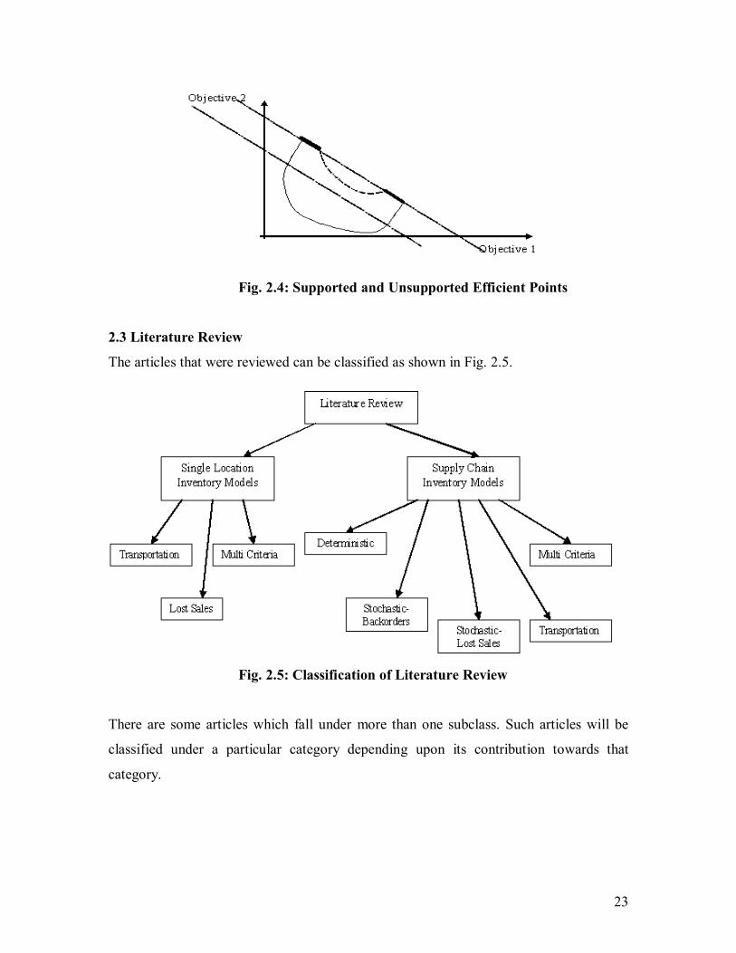
method. Such points are called unsupported efficient points. This is illustrated in Fig. 2.4.
The supported efficient points are the points that can be generated by the Pλ problem, and
they are represented by the darkened lines. The unsupported efficient points are
represented by the dashed lines.
23
Fig. 2.4: Supported and Unsupported Efficient Points
2.3 Literature Review
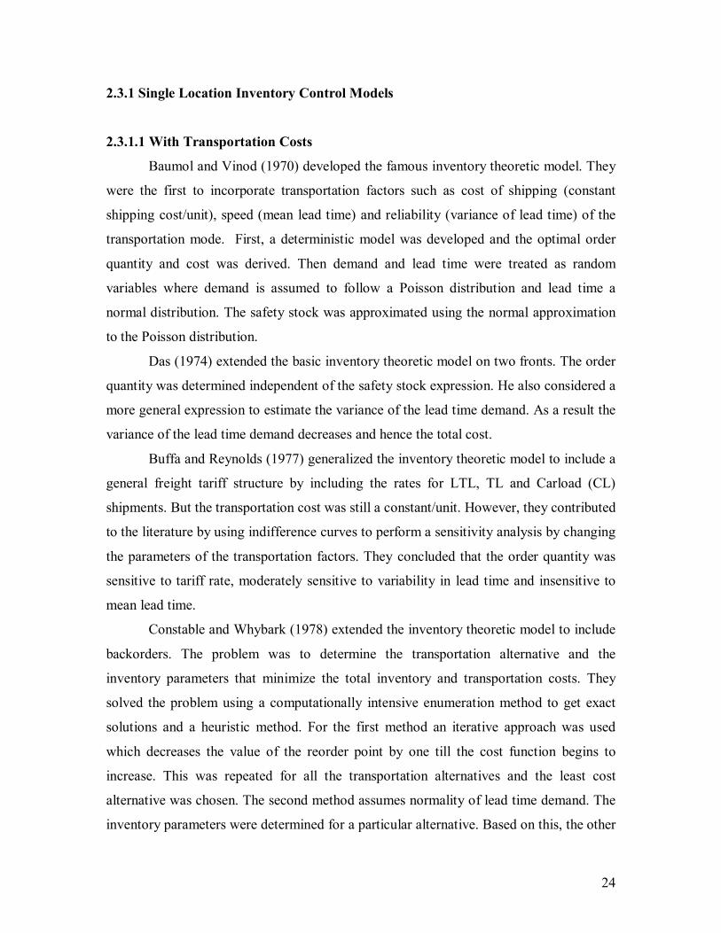
The articles that were reviewed can be classified as shown in Fig. 2.5.
Fig. 2.5: Classification of Literature Review
There are some articles which fall under more than one subclass. Such articles will be
classified under a particular category depending upon its contribution towards that
category.
24
2.3.1 Single Location Inventory Control Models
2.3.1.1 With Transportation Costs
Baumol and Vinod (1970) developed the famous inventory theoretic model. They
were the first to incorporate transportation factors such as cost of shipping (constant
shipping cost/unit), speed (mean lead time) and reliability (variance of lead time) of the
transportation mode. First, a deterministic model was developed and the optimal order
quantity and cost was derived. Then demand and lead time were treated as random
variables where demand is assumed to follow a Poisson distribution and lead time a
normal distribution. The safety stock was approximated using the normal approximation
to the Poisson distribution.
Das (1974) extended the basic inventory theoretic model on two fronts. The order
quantity was determined independent of the safety stock expression. He also considered a
more general expression to estimate the variance of the lead time demand. As a result the
variance of the lead time demand decreases and hence the total cost.
Buffa and Reynolds (1977) generalized the inventory theoretic model to include a
general freight tariff structure by including the rates for LTL, TL and Carload (CL)
shipments. But the transportation cost was still a constant/unit. However, they contributed
to the literature by using indifference curves to perform a sensitivity analysis by changing
the parameters of the transportation factors. They concluded that the order quantity was
sensitive to tariff rate, moderately sensitive to variability in lead time and insensitive to
mean lead time.
Constable and Whybark (1978) extended the inventory theoretic model to include
backorders. The problem was to determine the transportation alternative and the
inventory parameters that minimize the total inventory and transportation costs. They
solved the problem using a computationally intensive enumeration method to get exact
solutions and a heuristic method. For the first method an iterative approach was used
which decreases the value of the reorder point by one till the cost function begins to
increase. This was repeated for all the transportation alternatives and the least cost
alternative was chosen. The second method assumes normality of lead time demand. The
inventory parameters were determined for a particular alternative. Based on this, the other
25
transportation alternatives were evaluated. The least cost alternative was chosen and the
inventory parameters were recalculated. The heuristic results were very close to the
actual solution.
Lee (1986) extended the basic EOQ model to incorporate discounts in the freight
rates. He considered all units discount, incremental discount and the case of a stepwise
freight cost which is proportional to the number of trucks used. He developed an efficient
algorithm to solve the first case and modified it to solve the other two special cases.
Tyworth and Zeng (1998) used a sensitivity analysis approach to estimate the
effects of carrier in-transit time on total logistics cost and service. A single stocking point
following a continuous review policy faces stochastic demand. The lead time is assumed
to have two components: transit time which is a discrete random variable and a fixed
order processing time. Demand was assumed to be a gamma distributed random variable.
Fill rate was used as a service measure and is arbitrarily set to a value. To incorporate
transportation costs in the model, a curve was fit to the freight rates given the origin,
destination and class of freight. They concluded that a power function would work well
for the available data. This was implemented in a spreadsheet where the user can study
the effects of the various parameters on the total cost.
Swenseth and Godfrey (2002) used the inverse and adjusted inverse freight rate
function to determine the optimal order quantity. Based on these two functions the
authors developed a heuristic to determine when to over-declare a shipment as a TL or to
continue as a LTL shipment. This implies that in the former case the inverse function is
used and in the latter the adjusted inverse function is used.
2.3.1.2 Lost Sales
Smith (1977) determines inventory policies for a location following a (S,S-1)
policy, facing Poisson demand and any arbitrary distribution for lead times. A (S,S-1)
policy is a special case of a (S,s) policy wherein an order of one unit is placed when the
reorder point equals S-1 units. It is also called one-for-one ordering policy. He models the
system as a queue with multiple servers and uses Erlang�s loss formula to compute the
steady state distribution of the lead time demand. Using this, the steady state distribution
for inventory and shortages were derived.
26
Nahmias (1979) developed approximate solutions for a location following a
periodic review policy. He first extends the deterministic lead time lost sales case to
incorporate fixed cost for placing an order. The second extension was to accommodate
stochastic lead times. The third model accounts for partial backordering.
Archibald (1981) considered the inventory analysis of a single location for
demand following a compound Poisson process and constant lead times. An (S, s) policy
that is being continuously reviewed is assumed to be followed at the location. Excess
demand was treated as lost sales. Using a Markovian approach, an expression for the
average stationary cost was derived.
2.3.1.3 Multi-Criteria Inventory Control Theory
Brown (1961) was the first to suggest the treatment of the inventory control
problem as a multi-criteria problem. The two criteria used were the annual number of
orders and the quantity ordered per cycle.
Starr and Miller (1962) formulated the multi-item inventory control problem as a
bi-criteria problem for a single stocking point. They used the capital invested in inventory
and the annual number of orders as the two criteria. Using Lagrangian relaxation
technique they proved that the product of the two criteria is a constant. Based on this
result an optimal policy curve was developed which helps the decision maker in making
tradeoffs.
Gardner and Dannenbring (1979) extended the work of Starr and Miller (1962) to
a stochastic demand setting. In addition to the two criteria, they evaluated the customer
service objective as the third criteria. The optimal policy curve was replaced by an
optimal policy surface. A combination of Lagrangian relaxation and successive
approximation technique was used to locate the points on the optimal policy surface.
Agrell (1995) solved the stochastic inventory problem by using three criteria: 1)
expected annual cost. 2) annual number of stock-out occasions. 3) annual number of
items stocked-out. An interactive decision exploration method (IDEM) was used to solve
the problem. Local tradeoffs were determined by solving a generalized Lagrangian
problem. The decision maker had to decide whether he/she has to improve, maintain or

27
sacrifice a particular objective. An Excel-based tool was then developed to solve medium
range production planning problems.
2.3.2 Supply Chain Inventory Models
2.3.2.1 Deterministic Supply Chain Inventory Models
This section provides a review of some of the significant work done in single
warehouse multi-retailer type of systems.
Schwarz (1973) concluded that the optimal policy for a single warehouse multi-
retailer system was very complex since the order quantity varies with time even though
the demand is deterministic. He concentrated on a class of policies called the basic policy
and he showed that the optimal policy can be found in the set of basic policies. For the
single retailer case he proved that the single cycle policy is the optimal policy. This result
was not applicable for a more generalized system. A heuristic solution was proposed to
solve the general problem.
Roundy (1985) concluded the ineffectiveness of nested policies. He developed a
new class of policy called the power-of -two policies. The power-of-two restriction states
that the time between orders of a retailer is a power-of-two multiple of a base period. An
optimal solution to the relaxation of power-of-two formulation was derived. For a fixed
base period, the cost of the power-of-two policy was 6% above the cost of the optimal
policy whereas for a variable base period the cost was 2% above the cost of the optimal
policy.
Abdul-Jalbar et al. (2003) compared the single warehouse multi-retailer problem
operating under decentralized and centralized frameworks subjected to deterministic
demand. When the system is operating in a decentralized framework, the warehouse faces
time varying demand as the retailers order independently, and at different time periods.
Hence, the order quantity at the warehouse was found over a finite planning horizon. For
the centralized case the common replenishment time and different replenishment time
were evaluated. The parameters were sampled from two separate uniform distributions.
The number of instances where the decentralized case produced better results than the
centralized cases increased with increase in the number of retailers. Also, the
28
decentralized case was preferred when the costs at the retailers was significantly greater
than the cost at the warehouse.
Rangarajan and Ravindran (2005) introduced a base period policy for a
decentralized supply chain. This policy states that every retailer orders in integer
multiples of some base period, TB, which is arbitrarily set by the warehouse. The
warehouse problem is solved as a finite planning horizon model using Wagner-Whitin�s
model.
2.3.2.2 Stochastic Supply Chain Inventory Models with Backorder Assumption
Under this category the literature pertaining to (S,S-1) and (Q,r) policies are
covered. A (S,S-1) policy is a special case of a (S,s) policy wherein an order of one unit
is placed when the reorder point equals S-1 units. It is also called a one-for-one ordering
policy.
(S,S-1) Policies
Sherbrooke (1968) considered the case of a single warehouse supplying to several
downstream retailers, where the demand faced by the retailers follow a Poisson
distribution and stochastic lead times. The outstanding orders at the warehouse are
characterized as a Poisson distribution. This follows from the result of Palm�s theorem.
However, the same cannot be said about the outstanding orders at each retailer as they are
dependent on the inventory position at the warehouse. Sherbrooke approximates the
outstanding orders as a Poisson distribution which is characterized by the mean (single
parameter approximation).
Graves (1985) extended Sherbrooke�s (1968) work by characterizing the
outstanding orders at each retailer by using the mean and the variance (two-parameter
approximation). He then fits a negative binomial distribution to these parameters to
determine the ordering policy at each location.
Axsater (1990) demonstrated that the approximation of Sherbrooke (1968)
underestimates the number of backorders, while the two-parameter approximation of
Graves (1985) overestimates the number of backorders. Using the observation that an
item ordered by a location will be used to fill the Sth demand at that location and the
29
result that in a Poisson process the waiting time until the nth event follows an Erlang
distribution, he provides an exact solution by deriving expressions for expected costs at
the warehouse and the retailers. A recursive procedure is used to solve the problem
efficiently.
(Q,r) Policies
Deuermeyer and Schwarz (1981) developed an analytical model for predicting the
service level when the retailers face identical Poisson demand. The demand at the
warehouse is approximated as a stationary renewal process. They approximate the lead
time demand at the warehouse as a normal distribution. The actual lead time of a retailer
is the sum of the deterministic lead time plus the delay in meeting that retailer�s order as
a result of a stockout situation at the warehouse. They approximate the stochastic lead
time by determining only the expected delay. A simulation model was developed to
check the accuracy of the analytical model.
Svoronos and Zipkin (1988) consider the same problem as Deuremeyer and
Schwarz�s (1981). However, they use a different type of approximation to determine the
mean and variance of the lead time. Simulation results indicate that a shifted Poisson
distribution provided the best fit to the above parameters. In addition to quantifying the
mean delay at the warehouse due to a stockout, they also estimate the variance of the
delay.
Axsater (1993) provides an exact solution to the case of identical retailers in a
single warehouse multi-retailer system. The exact cost was derived as a weighted mean of
the costs for one-for-one ordering policies. This cost was evaluated by computing the
probability that a system demand will trigger a retailer�s order. Since the computational
effort involved in determining the probabilities is huge, he suggests the use of two
approximations. Based on a simulation study, it was concluded that the approximations
did give accurate results.
Forsberg (1996) provides an exact solution to the case of non-identical retailers.
He uses the same methodology of Axsater (1993) to derive the expression for the exact
cost. However, the probability computations were different as the previous method can
30
only be used for the case of two retailers. He computes the probability that the ith last
retailer order was triggered by the jth last customer demand.
Ganeshan (1999) presented near optimal solutions for a two stage decentralized
production-distribution system with multiple suppliers supplying a single warehouse,
which in turn supplied multiple retailers. The period demand at the retailer was assumed
to be a Poisson distribution. The period demand at the warehouse was then approximated
to a Poisson distribution provided that the number of the retailers is at least 20. The lead
time between each retailer and warehouse (fixed order processing time, fixed delay time
in case of shortages and random transit time) and the lead time between the warehouse
and each supplier (fixed order processing time and random transit time) are random
variables with known density functions. A linear logarithmic cost function was used to
estimate the transportation rates. These parameters were fed into a simulation model to
determine the backorder levels at the retailers, and it was found to be very close to the
actual fill rates set in the optimization model.
2.3.2.3 Stochastic Supply Chain Inventory Models with Lost Sales Assumption
Nahmias and Smith (1994) modeled the excess demand at the retailers in a two
echelon system as partial sales i.e. some customers are willing to wait with a known
probability, the others are treated as lost sales. Each location orders up to a base stock
every review period. External demand faced by the retailers followed a negative binomial
distribution. The demand at the warehouse is approximated as a Normal distribution.
Instantaneous replenishment was assumed throughout the paper.
Andersson and Melchirors (2001) extended the model developed by Sherbrooke
(1968) to the case where excess demand is considered as lost sales at the retailers. An
approximate cost function was derived for each retailer based on the assumption that the
lead times are i.i.d. The demand at the warehouse was approximated as a Poisson process
to derive the cost function at the warehouse. Using a heuristic, the solution on an average
was 0.4% above the optimal solution which was obtained using a simulation
31
2.3.2.4 Supply Chain Models with Transportation Costs
Perl and Sirisoponsilp (1988) analyzed the interdependence between facility
location, transportation and inventory decisions by developing an integrated model for a
distribution network. A good account of how strategic, tactical and operational decisions
in one function affected the various decisions in the other was outlined. The objective
function was to minimize the warehousing, trucking (between supplier and warehouse),
delivery (between warehouse and customer), in-transit inventory, cycle and safety stock
(at both the warehouse and customer) costs. Based on the service levels (probability of a
stockout), the inventory levels, the mode of transportation, assigning distribution centers
(DC) to suppliers and allocating customers to DCs were determined by the model. The
trucking cost comprised of a fixed cost and a variable cost which is inversely related to
the amount shipped. Nothing was mentioned about how the problem was solved.
Qu et al. (1999) developed a methodology where decisions regarding both
inventory and transportation could be made simultaneously. It was more of a shipment
consolidation problem where a central warehouse had to dispatch a truck to various
suppliers to collect different items. The total cost expression consisted of transportation
cost (stopover and routing costs) and inventory costs (ordering, holding and backorder
costs). The warehouse followed a modified periodic review policy where the fast moving
items (base items) were ordered every base period, and the remaining items were ordered
in integer multiples of the base period. The problem was solved by a decomposition
procedure. Two problems, the inventory master problem and the transportation sub-
problem were created. The solution was obtained by iterating between the master and the
sub-problem. The sub-problem reduces to a traveling salesman problem since the vehicle
was assumed to have infinite capacity. Transportation cost per unit distance was used.
Nozick and Turnquist (2001) developed an integrated framework that accounts for
facility, inventory and transportation costs with service levels at the customer zones. A
fixed charge model was developed in which an approximate inventory function was
embedded. This was based on an earlier work done by the authors, which approximates
the safety stock as a linear function of the number of facilities (distribution centers) for a
given stock-out rate under the condition that demand is a Poisson random variable. To
capture the fundamental tradeoff between service level and cost of opening new facilities,
32
they developed a multi-objective math program by introducing another objective which
minimized the uncovered demand. By assigning a weight to this objective, the
aforementioned tradeoff can be captured by increasing/decreasing the weights. They
suggested the use of any standard algorithm that solves the fixed charge problem to solve
this problem because of the same structure. However, neither actual freight rates nor
functions which emulate the actual freight rates were used.
Chan et al. (2002) considered a single warehouse-multiple retailer scenario where
the warehouse is supplied by a single supplier. They developed a finite horizon model for
time varying demand with a piecewise linear concave transportation cost structure for the
link between supplier and warehouse and a modified all unit discount structure (weight
breaks) between warehouse and retailers. They evaluated Zero Inventory Ordering (ZIO)
policies, i.e., the warehouse places an order only if the inventory level is zero (Wagner-
Whitin rule), which implies that the warehouse is a cross-docking facility. Upper bounds
were calculated on the cost of the ZIO policy in the case of time varying transportation
and stationary transportation costs. After the transformation, the problem was
reformulated as a shortest-path problem and solved using Dijkstra�s algorithm. However,
the problem becomes NP hard (non deterministic polynomial) when the number of
retailers increases. The problem was then formulated has an Integer Program (IP), which
could be solved only for small scale problems. Hence, a Linear Program (LP) based
heuristic was developed which gave quality solutions very quickly for large scale
problems.
Geunes and Zeng (2003) presented an approach to optimize inventory and
transportation costs when shortages occur at a warehouse which follows a periodic
review policy, while facing stochastic demand. Complete expediting, complete
backordering and a hybrid policy (partial backordering-partial expediting policy) were
evaluated. A maximum current demand needs to be shipped (MCDS) every period. The
warehouse used expedited shipping to ship the difference between MCDS and available
stock from the supplier. The rest of the demand is backlogged. Expressions for inventory
and transportation costs were developed. A heuristic approximation was used to solve the
problem since a mathematically tractable expression could not be developed for the
transportation cost. Results indicate that the hybrid policy outperforms the other policies
33
and, in some cases where the expediting cost was greater than the backlogging cost, the
solution recommended to follow a complete backordering policy. However, the authors
do not consider a systems approach i.e. they solved only the warehouse problem.
Toptal et al. (2003) extended the buyer-vendor (retailer-warehouse) problem
under deterministic demand by developing two models: 1) including inbound
transportation costs and 2) including inbound and outbound transportation costs at the
warehouse. The transportation cost structure included a fixed cost and a stepwise freight
cost that is proportional to the number of trucks used. Heuristics solutions were
developed for both the models, and worst case error bounds were 6% and 25% for model
1 and model 2, respectively. However, numerical analysis of a sample problem indicates
that the error in the heuristic solution was much less than 25% for model 2. The model,
however, would give accurate results for TL because of the transportation cost function.
Mason et al. (2004) built a mixed integer programming finite horizon model that
integrated inventory and transportation decision making considering time based service
levels into account for a service parts logistics industry under varying demand. The
problem setting consists of a single supplier supplying different parts to multiple
warehouses, which in turn supply to different customer zones. The problem was
formulated for three different inventory policies: 1) (s, S) policy, 2) Base stock policy,
and 3) (r, Q) policy. The model determined how much each warehouse ships to each
customer by which transportation mode in a time period. It also determined the reorder
points, order-up-to levels and the average inventory levels at each warehouse for all the
parts. A full factorial experiment was conducted by varying some of the parameters to
compare the dynamic model with a static one and the performances of the
aforementioned policies were evaluated. As expected, the dynamic model outperformed
the static model. In terms of the inventory policies, there was no significant difference
between (s, S) and (r, Q) policy. The base stock policy performed better than the other
two in the static case but not in the dynamic case.
Another stream of research in coordinating inventory-transportation decisions in
supply chain focuses on vehicle routing issues. A good overview of existing literature in
this area is given by Schwarz et al. (2004)

34
2.3.2.5 Multi-Criteria Supply Chain Inventory Models
Bookbinder and Chen (1992) considered a single warehouse single retailer
problem following a continuous review policy subjected to deterministic demand.
Assuming the availability of marginal cost information they developed two objectives: 1)
sum of ordering and holding costs and 2) fixed transportation cost for each shipment. The
analysis was then extended to probabilistic demand. Two cases were considered, one with
marginal cost information and the other without. In the first case the conflicting objective
functions were the sum of ordering and holding costs and the annual number of stock-out
occasions. The optimal order quantity and the reorder point were obtained by varying the
probability of stock-out. For case 2, in addition to the two objectives in case 1 fixed
transportation cost was the third objective. An interactive method based on Lagrangian
relaxation was used to solve the problem.
Thirumalai (2001) developed multi-criteria models for a serial supply chain where
each company is managed by an independent decision maker. In the deterministic
demand case the supply chain had two objectives, which were the annual number of
orders placed and the capital invested in inventory. A collaborative optimization
algorithm was suggested to bring the companies closer to supply chain efficiency. This
was then extended to the stochastic demand case. In addition to the two objectives, a third
objective that was considered was the probability of a stock-out.
DiFillipo (2003) extended the classic single warehouse multi-retailer problem by
using a multi-criteria approach that explicitly considered freight rate functions that
emulate actual freight rates for both centralized and decentralized cases. Under the
decentralized case, the fixed order and non-stationary order policies at the warehouse
were analyzed. Under the centralized case, common and different replenishment policies
were analyzed. To compare the different policies single objective problems were solved
using marginal cost information. Based on an example problem, both the policies under
the centralized case were dominated by the decentralized fixed order policy case. This
contradicts the well known result that centralized case outperforms the decentralized
case. However, the analysis was restricted to two retailers subjected to deterministic
demand.

35
2.4 Contributions of the Research
The contribution of this thesis is assessed chapter wise. Table 2.2 summarizes the
literature survey of deterministic base period inventory models.
Table 2.2: Contribution of Chapter 3
Author System Control Base Period
Effectiveness Grouping retailers
Roundy (1985) SWMR* Centralized Arbitrary ! x
Rangarajan & Ravindran (2005)
SWMR Decentralized Arbitrary ! x
This thesis SWMR Decentralized Specified ! !
Roundy (1985) and Rangarajan and Ravindran (2005) use an arbitrary value to set
the base period. Rangarajan and Ravindran (2005) addressed the issue that specifying the
base period incorrectly can lead to inferior solutions. In Chapter 3, the modified base
period policy is introduced wherein the base period is chosen based on sound intuitive
reasoning and validation from an executive of a Fortune 500 consumer products
company. This allows us to theoretically group retailers into clusters in terms of how
important they are to the warehouse. The effectiveness of the policy was tested by
developing theoretical bounds on the deviation from the optimal solution. The example
problem and case study (with real world data) indicates that the modified base period
policy performs really well for a wide range of data.
Table 2.3 summarizes the literature review associated with the deterministic
multi-criteria supply chain model with transportation costs in Chapter 4.
* Single Warehouse Multi Retailer

36
Table 2.3: Contribution of Chapter 4
Author Location System Criteria Transportation Costs
Brown(1961) Single - Multiple - Starr & Miller
(1962) Single - Multiple -
Thirumalai (2001)
Multiple Serial Multiple -
Chan et al. (2002)
Multiple SWMR Single Piecewise linear concave & modified
all unit discount Toptal et al.
(2003) Multiple Serial Single Stepwise cost
structure DiFillipo
(2003) Multiple SW2R� Multiple Continuous functions
This thesis Multiple SWMR Multiple Continuous functions
Brown (1961) and Starr and Miller (1962) treated the inventory problem from a
multi-criteria perspective for single locations facing deterministic demands. Thirumalai
(2001) and DiFillipo (2003) have treated the deterministic supply chain inventory
problem from a multi-criteria perspective. While Thirumalai�s work is restricted to serial
supply chains, DiFillipo�s work is restricted to a single warehouse two retailer system. In
Chapter 4, we extend the modified base period policy proposed in Chapter 3 to a multi-
criteria framework. The three criteria considered are capital invested in inventory, annual
number of orders placed and annual transportation costs.
Table 2.4 summarizes the relevant literature related to the stochastic multi-criteria
model with transportation costs developed in Chapter 5.
� Single Warehouse Two Retailers

37
Table 2.4: Contribution of Chapter 5
Author Location System Lead times BO/LS� Criteria Transportation Costs
Gardner & Dannenbring
(1979)
Single - - BO Multiple -
Deuermeyer & Schwarz
(1981)
Multiple SWMR Deterministic BO Single -
Svoronos & Zipkin (1988)
Multiple SWMR Deterministic BO Single -
Bookbinder &Chen(1992)
Multiple Serial Deterministic BO Single
Axsater (1993)
Multiple SWMR Deterministic BO Single -
Nahmias & Smith (1994)
Instantaneous LS Single -
Agrell (1995) Single - - BO Multiple - Forsberg (1996)
Multiple SWMR Deterministic BO Single -
Ganeshan (1999)
Multiple SWMR Stochastic BO Single Continuous functions
Thirumalai (2001)
Multiple Serial - BO Multiple -
Andersson & Melchirors
(2001)
Multiple SWMR Deterministic LS Single -
This thesis Multiple SWMR Stochastic LS & BO Multiple Continuous functions
Deuermeyer and Schwarz (1981), Svoronos and Zipkin (1988) and Ganeshan
(1999) provide an approximate approach to modeling and solving a single warehouse
multi-retailer system with identical stochastic demands. Ganeshan (1999) treats the lead
times as random variables. Axsater (1993) and Forsberg (1996) concentrate on
developing exact solutions for the identical and non-identical demands respectively. They
acknowledge that extending their work to the case of stochastic lead times is extremely
difficult. None of the above researchers consider the case of lost sales. Nahmias and
Smith (1994) consider the lost sales case for a periodic review system, while Andersson
and Melchirors (2001) consider the lost sales case for a one-for-one ordering policy.
� Backorders/Lost Sales
38
Bookbinder and Chen (1992) and Thirumalai (2001) have used a multi-criteria approach
to the backorders case while assuming that the lead time demand is normally distributed.
They treat cycle service level (CSL) as the criterion that measures customer satisfaction.
In Chapter 5, we develop a multi-criteria model that accounts for both stochastic non-
identical demands and random lead times. Fill rate (FR) is the fourth criterion and is used
to measure customer satisfaction. We cover both the lost sales and backorders case.
To summarize, there has been a lot of work done in joint inventory-transportation
decision making for single stocking points, both under the deterministic and stochastic
case. Researchers have used complex step functions as well as simple continuous
functions to model the freight rate costs. Multi-criteria techniques have also been used to
solve the inventory problem under both deterministic and stochastic setting for single
stocking points.
Multi-criteria optimization techniques have hardly been used in the field of supply
chain management. Given the nature of the problem (conflicting criteria) and the human
involvement in the decision making process, particularly in supply chains, there is a need
for paradigm shift from single objective methods to multiple criteria methods. Since the
DM analyzes the tradeoff information among the set of efficient solutions before the most
preferred solution is chosen, it is a more effective decision making tool. By choosing the
most preferred solution, the DM makes sure his/her preference information is
incorporated in the final solution.
In chapter 3, a single cost objective model is developed and solved that enables all
the companies in the supply chain to determine their invnentory ordering policies
efficiently. Using this model, a new inventory control policy is discussed, and its
effectiveness is tested. Also, a theoretical method is developed which enables the
warehouse to group retailers into clusters.
39
Chapter 3
A MODIFIED BASE PERIOD POLICY FOR A SINGLE WAREHOUSE MULTI-RETAILER
SYSTEM
3.1 Introduction
In a single warehouse multi-retailer system operating under decentralized control,
it is highly likely that each retailer is going to face different demands. Each retailer will
therefore order in different time periods, totally independent of one another. The
warehouse, in such a scenario faces an infinite horizon time varying demand. There has
to be some sort of an inventory control policy and coordination among the various
entities in the supply chain that will enable the warehouse to plan its inventory and at the
same time meet the demands of the retailers without deviating too much from their actual
requirements. Several such policies exist in literature, and they are listed next with
respect to the single warehouse multi-retailer system:
1. Integer policy (Crowston et al. (1973): The order quantity of the warehouse is an
integer multiple of the sum of the order quantity of the downstream retailers.
2. Basic Policy (Schwarz, 1973): A basic policy is one which satisfies the following
properties:
• A delivery is made to the warehouse only when the warehouse has zero
inventory and at least one retailer has zero inventory.
• A delivery is made to the retailer only when that retailer has zero
inventory.
• The deliveries made to a retailer during the ordering periods of the
warehouse are equal.
3. Myopic policy (Schwarz, 1973): Myopic policy is a special class of basic policy
where the original problem is split into N one warehouse one retailer problems.
4. Nested policy (Love, 1972): Nested policy is one in which each time the warehouse
orders all the retailers also place an order.
5. Stationary or fixed order policy (Schwarz, 1973): If the order quantity and the time
between orders for each retailer and the warehouse repeat itself then the policy is said
to be a stationary policy.

40
6. Single cycle policy (Schwarz, 1973): A single cycle policy is another class of basic
policy which is nested and stationary.
7. Power-of-two policy (Roundy, 1985): If the time period between orders of each
retailer is restricted to the power-of-two multiple of a base period, such a policy is
termed power-of-two policy.
8. Base period policy (Rangarajan and Ravindran, 2005): If the time period between
orders of each retailer is restricted to integer multiple of a base period, such a policy is
termed base period policy.
The power-of-two policy and the base period policy assume arbitrary value for the
base period, for example a week or a month. Incorrectly specifying the base period can
lead to inferior solutions at the retailer. To avoid this problem, we introduce a modified
base period policy wherein the base period is set by the warehouse, based on a suitable
performance measure. Following the notations we first discuss the economic order
quantity (EOQ) model and an equivalent formulation called the economic reorder interval
problem.
3.1.1 Notation
Data
Di � Annual demand faced by retailer i ∀ i=1,2,�, N
hi � Inventory holding cost at retailer ($/unit/year) i ∀ i=1,2,�, N
ai � Fixed order cost at retailer i ∀ i=1,2,�, N
Dw � Annual demand faced by the warehouse.
hw � Inventory holding cost at the warehouse ($/unit/year).
aw � Fixed order cost at the warehouse.
N- Number of retailers.
Variables
Qi � Order quantity of retailer i ∀ i=1,2,�, N.
Ti � Time between orders at retailer i ∀ i=1,2,�, N.
QW � Order quantity of the warehouse.
TW � Time between orders at the warehouse.

41
3.1.2 EOQ Problem
Consider the case of a single location. The notation defined previously can be
used without the subscript. Then, the EOQ problem is to determine Q that minimizes
annual inventory cost:
0QMin
≥ 2Qh
QDaZ += (3.1)
The optimal order quantity, haD2Q* = (3.2)
The optimal reorder interval, hD
a2DQT ** == (3.3)
The optimal cost, aDh2Z* = (3.4)
3.1.3 Economic Reorder Interval Problem
Eq. 3.1 can also be expressed in terms of the reorder intervals, T by using
DQT = as:
0TMin
≥gT
TaZ += (3.5)
where 2hDg =
Eq. 3.3 can be rewritten as gaT* = (3.6)
and Eq. 3.4 as ag2Z* = (3.7)
3.2 Problem Description
The supply chain system being modeled consists of a single warehouse supplying
a product to several retailers. A manufacturer owns the warehouse and replenishes it on a
regular basis. The system operated under a decentralized control. The goal is to
efficiently determine ordering policies for each retailer and the warehouse.

42
3.2.1 Assumptions
• Demand faced by the retailers is assumed to be deterministic and continuous. It is
further assumed that extraneous factors such as risk, seasonality, promotions, etc.
have been incorporated when the forecasts were determined.
• Marginal cost information such as ordering and inventory holding costs are
available.
• Instantaneous lead times between echelons.
3.2.2 Base Period Policy
This policy was introduced by Rangarajan and Ravindran (2005) for a
decentralized supply chain. This policy states that every retailer orders in integer
multiples, n of some base period, TB, which is arbitrarily set by the warehouse. This
condition is incorporated into the economic reorder interval problem (Section 3.1.3) as
follows:
0TMin
≥gT
TaZ +=
s.t. BnTT = (3.8)
1n ≥ and integer.
A line search method is used to determine the optimal integer values, n. It is also
shown that the policy guaranteed error bounds within 6% of the EOQ policy provided the
base period is chosen carefully. The warehouse problem is solved as a finite planning
horizon model using Wagner-Whitin model (Wagner and Whitin, 1958).
3.3 Modified Base Period Policy
This section introduces the modified base period policy. This policy differs in one
important aspect: the base period, TB is no longer set arbitrarily.
3.3.1 Model Formulation
Under the modified base period policy each retailer starts of by solving Eq. 3.1 or
Eq. 3.5. This is called Problem (Ri). The output (optimal reorder interval) is passed on to
the warehouse. The warehouse identifies a base retailer or a set of base retailers. A base

43
retailer(s) is one who orders most frequently or, equivalently, has the least reorder
interval among all the retailers. Instead of arbitrarily specifying the base period, the
warehouse sets the base period as the reorder interval of the base retailer(s).
*iiB TMinT = (3.9)
where *iT is the economic reorder interval for retailer �i� .
The other retailers or the set of non-base retailers order in integer multiples of the
base period given by Eq. 3.9, i.e., these retailers have to incorporate Eq. 3.8 to Problem
(Ri), where TB is determined by the warehouse using Eq. 3.9. This problem is called the
Modified Retailer�s problem denoted by Problem (MRi) and is given as:
Problem (MRi)
0Ti
Min≥ ii
i
ii Tg
TaZ +=
Bii TnT:.t.s =
1ni ≥ and integer
3.3.2 Setting TB: A Different Perspective
An intuitive reason to set the base period as in Eq. 3.9 is as follows: The
warehouse receives its first order at a time period given by *ii
TMin . This implies that none
of the other retailers are going to place an order before *ii
TMin . Hence, there is no need to
set the base period below the value given by Eq. 3.9. Now, consider the case where TB is
set such that *iiB TMinT > . This means that the orders placed by the set of base retailers
will not be met on time. Hence, there is no point in setting *iiB TMinT > .
3.3.3 Another Interpretation of TB
In addition to the interpretation of TB in Section 3.3.1, another interpretation is
warranted. TB can also be thought of as a throughput measure. Throughput is a
performance metric used in scheduling jobs in a machine shop to indicate the rate at
which a part(s) exits the machine shop after finishing all the machining requirements.
Increasing throughput increases the efficiency of the shop by decreasing WIP (Work In-
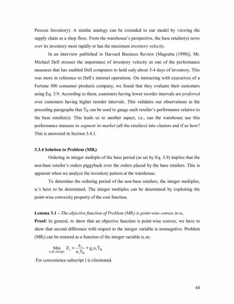
44
Process Inventory). A similar analogy can be extended to our model by viewing the
supply chain as a shop floor. From the warehouse�s perspective, the base retailer(s) turns
over its inventory most rapidly or has the maximum inventory velocity.
In an interview published in Harvard Business Review (Magretta (1998)), Mr.
Michael Dell stresses the importance of inventory velocity as one of the performance
measures that has enabled Dell computers to hold only about 3-4 days of inventory. This
was more in reference to Dell�s internal operations. On interacting with executives of a
Fortune 500 consumer products company, we found that they evaluate their customers
using Eq. 3.9. According to them, customers having lower reorder intervals are preferred
over customers having higher reorder intervals. This validates our observations in the
preceding paragraphs that TB can be used to gauge each retailer�s performance relative to
the base retailer(s). This leads us to another aspect, i.e., can the warehouse use this
performance measure to segment its market (all the retailers) into clusters and if so how?
This is answered in Section 3.4.1.
3.3.4 Solution to Problem (MRi)
Ordering in integer multiple of the base period (as set by Eq. 3.9) implies that the
non-base retailer�s orders piggyback over the orders placed by the base retailers. This is
apparent when we analyze the inventory pattern at the warehouse.
To determine the ordering period of the non-base retailers, the integer multiples,
ni�s have to be determined. The integer multiples can be determined by exploiting the
point-wise convexity property of the cost function.
Lemma 3.1 � The objective function of Problem (MRi) is point-wise convex in ni.
Proof: In general, to show that an objective function is point-wise convex, we have to
show that second difference with respect to the integer variable is nonnegative. Problem
(MRi) can be restated as a function of the integer variable ni as:
egerint,1ni
Min≥ Bii
Bi
ii Tng
TnaZ +=
For convenience subscript i is eliminated.

45
BB
gnTnT
a)n(Z +=
BB
T)1n(gT)1n(
a)1n(Z +++
=+
Computing the first difference:
)n(Z)1n(Z)n(Z −+=∆
BB
gT)1n(nT
a ++
−=
Similarly,
BB
gT)2n)(1n(T
a)1n(Z +++
−=+∆
Computing the second difference:
)n(Z)1n(Z)1n(Z2 ∆−+∆=+∆
++−
+=
)2n)(1n(1
)1n(n1
Ta
B
++=
)2n)(1n(n2
Ta
B
> 0
■
Theorem 3.1- The optimal integer value ni for each retailer is the smallest integer that
satisfies the following condition:
2
B
*i
ii TT
)1n(n
≥+ (3.10)
Proof: The optimal integer multiple is determined by finding the smallest integer such
that first difference is non-negative.
0)n(Z)1n(Z)1n(Z ≥−+=+∆
0gT)1n(nT
aB
B≥+
+−⇒
BB
gT)1n(nT
a ≤+
⇒

46
2
B
*
TT)1n(n
≥+⇒
■
The right hand side (RHS) of Eq. 3.10 is always greater than 1 due to Eq. 3.9. The
ratio B*i TT indicates how often each non-base retailer orders relative to the base
retailers. It can also be thought of as how each non-base retailer performs in comparison
to the base retailer in terms of inventory turns. We use *iB TT instead of B
*i TT in the
rest of the analysis.
3.4 Analysis of the Modified Base Period Policy
In this section we analyze the modified base period policy in more detail. The first
part of the analysis deals with developing a theoretical framework to classify retailers
into clusters. In the second part, bounds are developed on the deviation from the EOQ
solution as a result of following this policy for the retailers.
3.4.1 Grouping Retailers
Since the concepts of revenue management are becoming prominent in supply
chain management, it is important for the warehouse to differentiate among its customers
by providing different quality of service in order to maximize its revenues.
We can use an analogy from Pareto�s principle: 80% of the revenue is generated
from 20% of the customers. Hence, the warehouse has to provide better service to these
retailers, e.g., meeting demand requirements, on time delivery, etc. To do this, the
warehouse has to first segment its market into groups or clusters based on several
performance measures.
As mentioned in Section 3.3.3., TB as set by Eq. 3.9 is used by a Fortune 500
company to measure the performance of their retailers. We use this performance metric
along with the result of Problem (MRi) as given by Eq. 3.10 to theoretically derive results
that help the warehouse in grouping retailers into clusters.
It is of interest to find the breakpoints, i.e., at what values of *B TT does the
value of n change. This can be achieved by solving the equality form of Eq. 3.10:

47
2
B
*
TT
)1n(n
=+
)1n(n
1TT
*B
+=
The value of n remains unchanged between two consecutive breakpoints. We
refer to this as the breakpoint interval. For example, the breakpoint interval for n=2
is
21,
61 . At 61TT *
B = , n changes from 3 to 2 and at 21TT *B = , n becomes
1.
More specifically, we can use these breakpoint intervals to group retailers into a
cluster. For example, if *B TT for a set of retailers fall in the interval
1,2
1 , then they
can be grouped together into cluster 1§. If the ratios fall in the interval
21,
61 , then it
is grouped into cluster 2, and so on.
We believe that these results can be used in conjunction with other financial
metrics, e.g., gross margins, to more effectively group retailers. Based on this, the
warehouse can then decide how best to serve each group of retailers.
3.4.2 Effectiveness of the Policy
Being a decentralized system, each retailer would like to have their ordering
policy as close to the EOQ policy as possible. The base retailer�s ordering policy is going
to be the EOQ solution itself. It is important to know how much the solution for the set of
non-base retailers deviate from the optimal solution.
Since the objective function of Problem (MRi) is point-wise convex, we have to
find the smallest integer where the objective value starts to increase, i.e.,
}T)1n{(Z}nT{ZT)1n{(Z BBB +≤≥−
Consider }T)1n{(Z}nT{Z BB +≤
§ The base retailers are grouped in cluster 1 as well.

48
BB
BB
T)1n(gT)1n(
agnTnT
a +++
≤+⇒
BB
gT)1n(nT
a ≤+
⇒
T)1n(T
)T(
B
2*≤
+⇒ (Using Eq. 3.6 and Eq. 3.8) (3.11)
Similarly it can be shown that )1n(T
)T(TB
2*
−≤ (3.12)
Eq. 3.11 and Eq. 3.12 implies that )1n(T
)T(T)1n(T
)T(
B
2*
B
2*
−≤≤
+ (3.13)
Eq. 3.13 provides a lower and upper bound on the reorder interval of a retailer. The next
step is to compute the objective values at these two bounds
Let)1n(T
)T(LB
2*
+= and
)1n(T)T(U
B
2*
−=
)1n(T)T(g
)1n(T)T(aZ
B
2*
B2*L +
++
=
)1n(T
a)1n(gTB
B +++= (Using Eq. 3.6)
+++=
)1n(1
TT)1n(
TT
21
ZZ
B
*
*B
*L (Multiplying and dividing by ag2 ) (3.14)
Similarly,
−+−=
)1n(1
TT)1n(
TT
21
ZZ
B
*
*B
*U (3.15)
The maximum of Eq. 3.14 and Eq. 3.15 is the worst case deviation bound from
the EOQ solution when following the modified base period policy and is given as:
−+−
+++≤
)1n(1
TT)1n(
TT
21,
)1n(1
TT)1n(
TT
21Max
ZZ
B
*
*B
B
*
*B
* (3.16)
This bound could have been derived such that it is independent of TB as given by
Rangarajan and Ravindran (2005). Here, the bound has been deliberately derived with TB
so as to show the impact of *B TT on the deviation bounds. This bound is valid for n ≥ 2
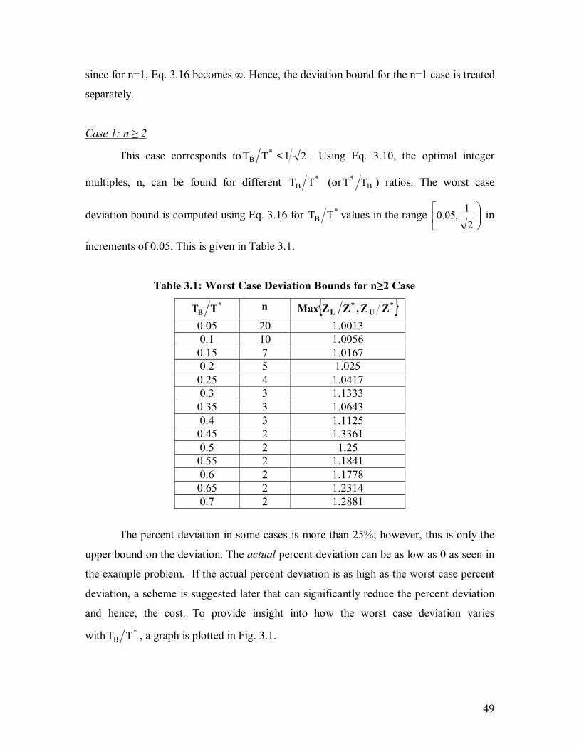
49
since for n=1, Eq. 3.16 becomes ∞. Hence, the deviation bound for the n=1 case is treated
separately.
Case 1: n ≥ 2
This case corresponds to 21TT *B < . Using Eq. 3.10, the optimal integer
multiples, n, can be found for different *B TT (or B
* TT ) ratios. The worst case
deviation bound is computed using Eq. 3.16 for *B TT values in the range
2
1,05.0 in
increments of 0.05. This is given in Table 3.1.
Table 3.1: Worst Case Deviation Bounds for n≥2 Case *
B TT n { }*U
*L ZZ,ZZMax
0.05 20 1.0013 0.1 10 1.0056 0.15 7 1.0167 0.2 5 1.025 0.25 4 1.0417 0.3 3 1.1333 0.35 3 1.0643 0.4 3 1.1125 0.45 2 1.3361 0.5 2 1.25 0.55 2 1.1841 0.6 2 1.1778 0.65 2 1.2314 0.7 2 1.2881
The percent deviation in some cases is more than 25%; however, this is only the
upper bound on the deviation. The actual percent deviation can be as low as 0 as seen in
the example problem. If the actual percent deviation is as high as the worst case percent
deviation, a scheme is suggested later that can significantly reduce the percent deviation
and hence, the cost. To provide insight into how the worst case deviation varies
with *B TT , a graph is plotted in Fig. 3.1.
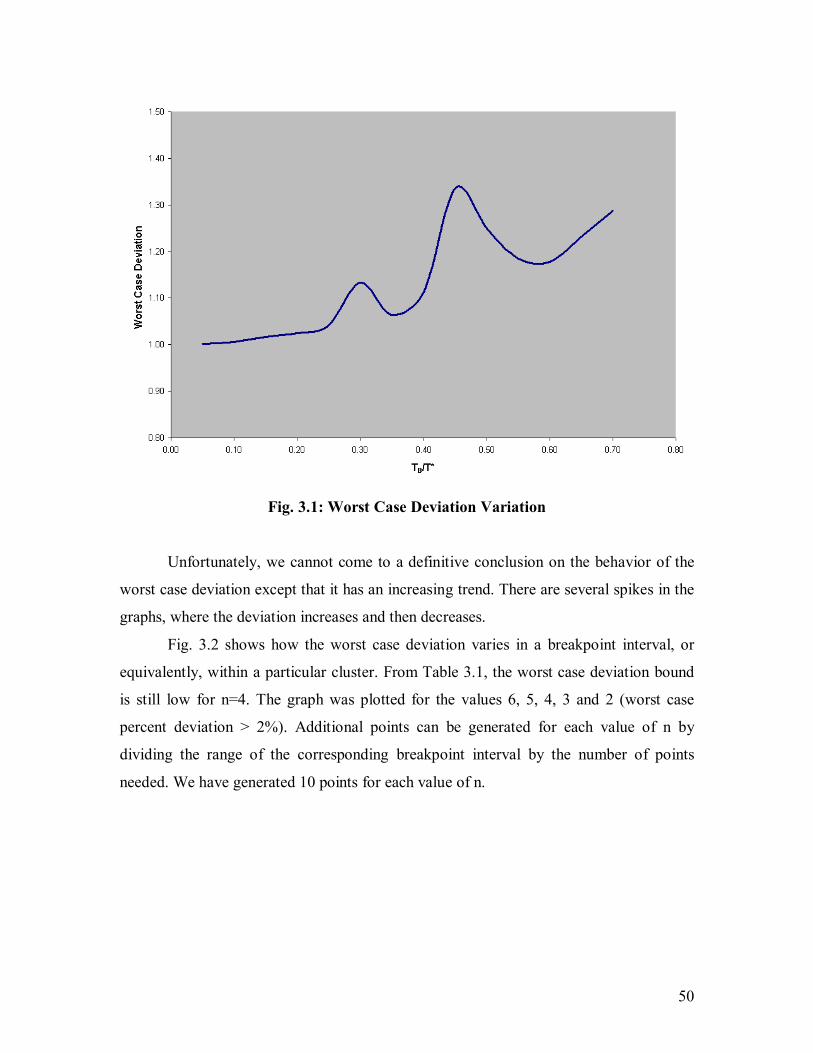
50
Fig. 3.1: Worst Case Deviation Variation
Unfortunately, we cannot come to a definitive conclusion on the behavior of the
worst case deviation except that it has an increasing trend. There are several spikes in the
graphs, where the deviation increases and then decreases.
Fig. 3.2 shows how the worst case deviation varies in a breakpoint interval, or
equivalently, within a particular cluster. From Table 3.1, the worst case deviation bound
is still low for n=4. The graph was plotted for the values 6, 5, 4, 3 and 2 (worst case
percent deviation > 2%). Additional points can be generated for each value of n by
dividing the range of the corresponding breakpoint interval by the number of points
needed. We have generated 10 points for each value of n.
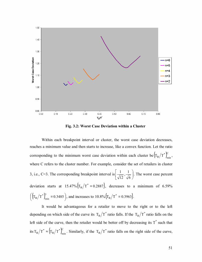
51
Fig. 3.2: Worst Case Deviation within a Cluster
Within each breakpoint interval or cluster, the worst case deviation decreases,
reaches a minimum value and then starts to increase, like a convex function. Let the ratio
corresponding to the minimum worst case deviation within each cluster be ( )Cmin
*B TT ,
where C refers to the cluster number. For example, consider the set of retailers in cluster
3, i.e., C=3. The corresponding breakpoint interval is
61,
121 . The worst case percent
deviation starts at 15.47% ( )2887.0TT *B = , decreases to a minimum of 6.59%
( )
= 3485.0TT
3
min*
B , and increases to 10.8% ( )3963.0TT *B = .
It would be advantageous for a retailer to move to the right or to the left
depending on which side of the curve its *B TT ratio falls. If the *
B TT ratio falls on the
left side of the curve, then the retailer would be better off by decreasing its T* such that
its ( )Cmin
*B
*B TTTT ≈ . Similarly, if the *
B TT ratio falls on the right side of the curve,

52
then the retailer would be better off by increasing its T*. For example, by moving from
2887.0TT *B = to 3485.0 a cost savings of approximately 10% can be achieved, which
is a significant reduction.
Case 2: n = 1
The integer multiple n becomes 1 for *B TT ratios that fall in the range
1,2
1 .
This implies that the ordering period for the retailers whose *B TT ratio falls in the
abovementioned range will be set as the base period. The deviation for this case is
derived by computing the ratio of the cost when the ordering period is TB to the cost
obtained by the EOQ solution:
ag2gTTa
ZZ BB
*+=
ag
2T
ga
T21 B
B+=
+= *
*
21
TT
TT B
B (3.17)
Using Eq. 3.17, the deviation is computed for ratios within the range
1,2
1 in
increments of 0.05 and is plotted in Fig. 3.3.
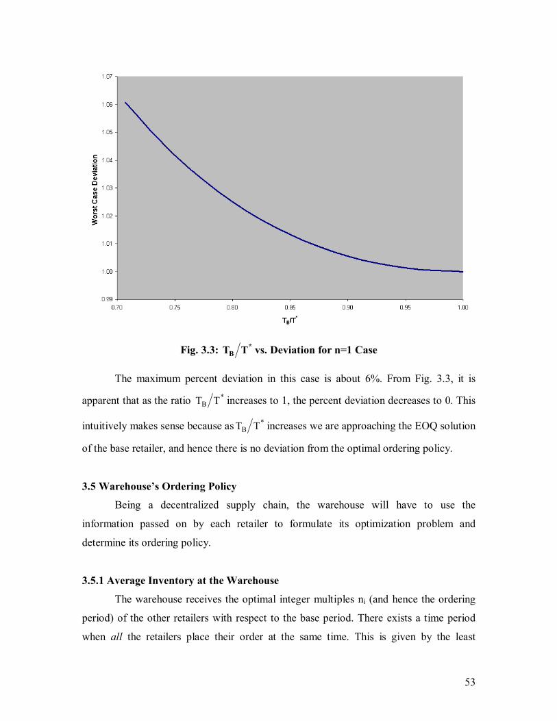
53
Fig. 3.3: *B TT vs. Deviation for n=1 Case
The maximum percent deviation in this case is about 6%. From Fig. 3.3, it is
apparent that as the ratio *B TT increases to 1, the percent deviation decreases to 0. This
intuitively makes sense because as *B TT increases we are approaching the EOQ solution
of the base retailer, and hence there is no deviation from the optimal ordering policy.
3.5 Warehouse�s Ordering Policy
Being a decentralized supply chain, the warehouse will have to use the
information passed on by each retailer to formulate its optimization problem and
determine its ordering policy.
3.5.1 Average Inventory at the Warehouse
The warehouse receives the optimal integer multiples ni (and hence the ordering
period) of the other retailers with respect to the base period. There exists a time period
when all the retailers place their order at the same time. This is given by the least

54
common multiple of the reorder intervals, BN21N21 T)n,...,n,n(M.C.L)T,...,T,T(M.C.L = .
This also corresponds to the smallest reorder period of the warehouse. Then, the number
of orders that each retailer places during the smallest reorder period of the warehouse,
denoted by mi can be computed as:
i
N21
i
N21i n
)n,...,n,n(M.C.LT
)T,...,T,T(M.C.Lm == i∀ (3.18)
These concepts are illustrated with the help of an example. Consider a warehouse
supplying the product to three different retailers. Each retailer�s inventory follows a saw
tooth pattern and has the Zero Inventory Ordering (ZIO) property. Retailer 1 places an
order every base period, Retailer 2 every two base periods, and Retailer 3 every three
base periods. Assume the base period TB is 1 time unit. The ratios ni are n1 = 1, n2 = 2,
and n3 =3. The time when all the retailers place their order
is 6)3,2,1(M.C.LT)n,n,n(M.C.L B321 == time units. The number of orders placed by
Retailer 1, Retailer 2 and Retailer 3 are m1=6, m2=3 and m3=2, respectively, during 6
time units. The inventory pattern for the 3 retailers is shown in Fig. 3.4.
Fig. 3.4: Inventory Pattern of the Retailers
55
Let )n,...,n,n(M.C.L N21=τ (3.19)
Hence, the general relationship:
BNN2211 TTm...TmTm τ=== (3.20)
The warehouse places an order once every τTB periods or in integer multiples of τTB
periods. Hence, the time between warehouse orders, denoted by TW, is given by:
)T(T BW τδ= where 1≥δ and integer (3.21)
Hence, the number of orders placed by each retailer between warehouse orders is δmi i∀ .
The annual demand faced by the warehouse is given by:
∑=
=N
1iiW DD (3.22)
Substituting Eq. 3.21 and Eq. 3.22 in QW=TWDW:
∑=
τδ=N
1iiBW D)T(Q
∑=
δ=N
1ii
i
ii D
DQm
∑=
δ=N
1iiiQm (3.23)
where Qi�s are the retailer order quantities.
The next step is to derive an expression for the average inventory in the
warehouse. Based on the one warehouse three retailer example given earlier (see Fig.
3.4.) an expression for the average inventory at the warehouse is derived. This expression
is then generalized for the N retailer case. For the example, δ=1 and TW=6 time units.

56
Fig. 3.5: Inventory Pattern of the Warehouse
Q1+Q2+Q3
Q1
Q1+Q2
Q1+Q3
Q1+Q2
Q1
QW -Q1+Q2+Q3

57
Fig. 3.5 illustrates the inventory pattern in the warehouse. Clearly, the inventory
at the warehouse does not follow a triangular saw tooth pattern. Let us assume that the
retailers and the warehouse have zero inventories at the beginning of the cycle. The
warehouse receives QW units at the beginning of the cycle. All three retailers place their
orders for Q1, Q2 and Q3. These orders are shipped out instantly. The inventory at the
warehouse drops to QW � Q1� Q2� Q3. After one time period (TB), only Retailer 1 places
an order. The inventory at the warehouse drops to QW � 2Q1� Q2� Q3. After two time
periods, Retailer 1 and Retailer 2 place orders. The inventory at the warehouse further
reduces to QW � 3Q1� 2Q2� Q3. This process continues till the inventory drops down to
zero at the end of period 6. At this moment the warehouse places another order and the
inventory level rises to QW and this process repeats itself. Note that the warehouse still
follows a fixed order policy.
Based on Fig. 3.5 the average inventory at the warehouse denoted by WQ is:
(QW � Q1� Q2� Q3)TB + (QW � 2Q1� Q2� Q3)TB + (QW � 3Q1� 2Q2� Q3)TB + (QW � 4Q1� 2Q2� 2Q3)TB + (QW � 5Q1� 3Q2� 2Q3)TB + (QW � 6Q1� 3Q2� 2Q3)TB
=WQ ____________________________________________________________________________________________________________ 6TB
( ) ( ) ( )
++++++++
−=6
636426...2 33222111 QQQQQQQQQW
( ) ( ) ( )
++++++++
−=6
233226...21 33222111 QQQQQQQQQW
++−=
23
22
7 32
1 QQ
QQW
The above expression is the average inventory at the warehouse for a specific
example. Observing the expression below, a pattern emerges:
( ) ( ) ( )
++++++++
−=6
233226...21 33222111 QQQQQQQQQQ WW (3.24)
In the numerator, the numbers 1, 2 and 3 outside the three summations correspond
to n1, n2 and n3. The coefficient of the last term in the first summation corresponds to m1.
Similarly, the coefficient of the last term in the second and the third summations
corresponds to m2 and m3. The denominator represents the smallest ordering cycle of the
warehouse.
58
Let δ=2. Then, the time between orders at the warehouse is 12. The warehouse
does not have to place an order at period 6 as shown in Fig. 3.5 since inventory has not
reached zero. Inventory continues to deplete, and it reaches zero at period 12. At this
instant the warehouse places an order, and the inventory level rises to QW. The number of
orders placed by Retailer 1, Retailer 2 and Retailer 3 are 12(2*6), 6(2*3) and 4(2*2),
respectively. Then Eq. 3.24 can be easily modified as:
++−=
(2)(6))4Q +�+2Q3(Q+)6Q+�+2Q 2(Q+)12Q+�+2Q +(Q 1 333222111
WW QQ (3.25)
Hence, Eq. 3.25 for the three retailer case can be generalized as:
δτ
δδδ−=
)Qm+�+2Q +(Qn+)Qm+�+2Q +(Qn+)Qm+�+2Q +(QnQQ 333332222211111
WW
δτ
δδδ−=
)m+�+2 +(1Qn+)m+�+2 +(1Qn+)m+�+2 +(1QnQ 333222111
W
δτ
+δδ+δδ+δδ−=
2)1m(mQn+)1m(mQn+1)m(mQn
Q 333322221111W
+δ−= ∑
=
3
1i 321
iiiiW )n,n,LCM(n
1)m(mQn21Q [Using Eq. 3.19]
+δ−= ∑
=
3
1i i
iiiW m
1)m(mQ21Q [Using Eq. 3.18]
+δ−= ∑
=
3
1iiiW 1)m(Q
21Q
This expression is the average inventory at the warehouse for the three retailer case. The
average inventory expression at the warehouse can be generalized for the N retailer case
as:
+δ− ∑
=
N
1iiiW 1)m(Q
21Q (3.26)
Consider the case of a serial supply chain, i.e., N=1, and δ =1. Then, Eq. 3.26
simplifies to )1(21
11 +− mQQW . This is the same result obtained by Thirumalai (2001) for
a serial supply chain when the warehouse orders in integer multiple of the retailer.
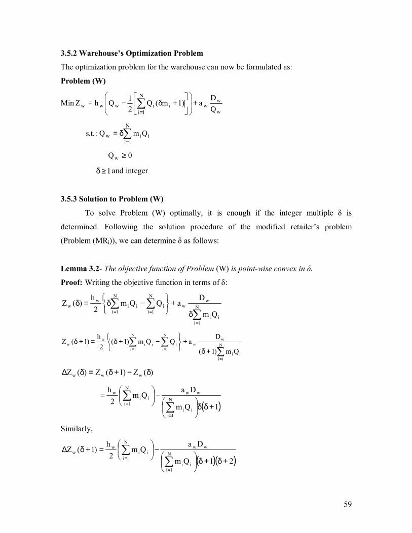
59
3.5.2 Warehouse�s Optimization Problem
The optimization problem for the warehouse can now be formulated as:
Problem (W)
Minw
ww
N
1iiiwww Q
Da1)m(Q
21QhZ +
+δ−= ∑
=
∑=
δ=N
1iiiw QmQ:.t.s
0Qw ≥
1≥δ and integer
3.5.3 Solution to Problem (W)
To solve Problem (W) optimally, it is enough if the integer multiple δ is
determined. Following the solution procedure of the modified retailer�s problem
(Problem (MRi)), we can determine δ as follows:
Lemma 3.2- The objective function of Problem (W) is point-wise convex in δ.
Proof: Writing the objective function in terms of δ:
∑∑∑
=
== δ+
−δ=δ N
1iii
ww
N
1ii
N
1iii
ww
Qm
DaQQm
2h
)(Z
∑∑∑
=
== +δ+
−+δ=+δ N
1iii
ww
N
1ii
N
1iii
ww
Qm)1(
DaQQm)1(
2h
)1(Z
)(Z)1(Z)(Z www δ−+δ=δ∆
( )1Qm
DaQm
2h
i
N
1ii
wwi
N
1ii
w
+δδ
−
=
∑∑
=
=
Similarly,
( )( )21Qm
DaQm
2h
)1(Z
i
N
1ii
wwi
N
1ii
ww
+δ+δ
−
=+δ∆
∑∑
=
=
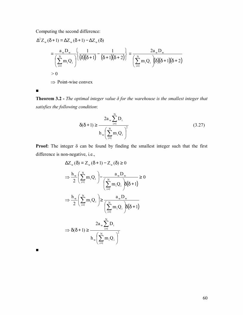
60
Computing the second difference:
)(Z)1(Z)1(Z www2 δ∆−+δ∆=+δ∆
( )( ) ( )( )
+δ+δ−
+δδ
=
∑=
211
11
Qm
Da
i
N
1ii
ww
( )( )( )21Qm
Da2N
1iii
ww
+δ+δδ
=
∑=
> 0
⇒ Point-wise convex
■
Theorem 3.2 - The optimal integer value δ for the warehouse is the smallest integer that
satisfies the following condition:
2
i
N
1iiw
N
1iiw
Qmh
Da2)1(
≥+δδ
∑
∑
=
= (3.27)
Proof: The integer δ can be found by finding the smallest integer such that the first
difference is non-negative, i.e.,
0)(Z)1(Z)(Z www ≥δ−+δ=δ∆
( )0
1Qm
DaQm
2h
i
N
1ii
wwi
N
1ii
w ≥+δδ
−
⇒
∑∑
=
=
( )1Qm
DaQm
2h
i
N
1ii
wwi
N
1ii
w
+δδ
≥
⇒
∑∑
=
=
2
i
N
1iiw
N
1iiw
Qmh
Da2)1(
≥+δδ⇒
∑
∑
=
=
■

61
3.6 Algorithm for the Modified Base Period Policy
Step 1: Each retailer solves its own Problem (Ri) (EOQ model). The optimal reorder
interval for each retailer is found using ii
i*i Dh
a2T = (see Eq. 3.3). Each retailer passes
this information to the warehouse.
Step 2: The warehouse identifies the base period (and hence the set of base retailers)
using *iiB TMinT = (see Eq. 3.9). The set of non-base retailers have to solve Problem
(MRi), which includes the constraint that their ordering period is an integer multiple of
the base period.
Step 3: The optimal integer values for the non-base retailers can be determined by finding
the smallest integer that satisfies 2
B
*i
ii TT
)1n(n
≥+ (see Eq. 3.10). Then, the reorder
intervals can be determined using Bii TnT = (see Eq. 3.8).
Step 4: Each retailer calculates the actual percent deviation from their EOQ solution
as ( ) *i
*iii ZZZ −=ε .
Step 5: Is mini d≤ε ? where, dmin is the minimum deviation that is acceptable to the
retailer. If yes, Go to Step 6, else go to Step 8.
Note: The dmin value is set by the retailer.
Step 6: Pass on the corresponding order information to the warehouse.
Step 7: Using 2
i
N
1iiw
N
1iiw
Qmh
Da2)1(
≥+δδ
∑
∑
=
= (see Eq. 3.27), the warehouse determines its
optimal integer δ and hence, its reorder interval.

62
Step 8: If mini d>ε , then the retailer informs the warehouse about the large deviation from
its EOQ solution. The warehouse can use Fig. 3.2 to indicate in which direction the
retailer should move so as to decrease the deviation.
Step 9: Repeat Step 8 until the condition mini d≤ε is satisfied. Go to Step 6.
This procedure is summarized as a flowchart in Fig. 3.4, where the dotted lines
indicate the flow of information.
Fig. 3.4: Flow Chart of the Modified Base Period Policy
3.7 Final Comments on the Modified Base Period Policy
Though it appears initially that the warehouse is the more dominant player in the
supply chain since the non-base retailers are made to order in integer multiples of a base
period also set by the warehouse, it is not the case. In fact the warehouse steers each
retailer according to the scheme suggested in Section 3.3.2., which results in significant
cost reductions for the retailer. The retailer is also allowed the option of setting a
minimum acceptable deviation from its optimal solution which the warehouse has to

63
necessarily meet. If the warehouse is unable to meet this requirement using the scheme
suggested, it can offer purchasing discounts to the concerned retailer(s).
This procedure is actually similar to the Vendor Managed Inventory (VMI). As
the name suggests, VMI deals with the vendor (warehouse) managing the ordering
decisions at the customers (retailers). This was first pioneered by the world�s biggest
retailer, Walmart. Thus, contrary to beliefs giant retailers like Walmart are not inflexible
in accepting changes to their ordering policies. Walton (2005) writes that Walmart is
open to changes in its ordering schedule as long as there are benefits for both parties
involved.
From the warehouse�s perspective, it has better visibility of all the retailers
ordering process. We already noted that the orders of the non-base retailers piggyback
over the base retailers. Also, all the retailers within a particular cluster place an order at
the same time. As a result, the warehouse receives an aggregated order of at least one
cluster of retailers every base period. Aggregating orders leads to achievement of
economies of scale at the warehouse. This would result in reducing significantly the order
processing and transportation costs.
Based on the preceding paragraphs, it is clear that this control policy is more of a
collaborative rather than a compromising approach due to the interactions between the
retailers and the warehouse. Moreover, there is no dominant player in the supply chain
and hence, should result in a �win-win� situation for all the companies in the system.
3.8 Example Problem
An example problem consisting of a single warehouse and three retailers is
considered to explain the methodology developed in the previous sections. The data is
provided in Table 3.2.
Table 3.2: Data for Example Problem
Demand (Di) Order cost (ai) Holding cost (hi) Retailer 1 800 units $42 $48 Retailer 2 525 units $100 $21 Retailer 3 415 units $52 $28
Warehouse $37 $8

64
Step 1: Each retailer solves Problem(R), i.e., the EOQ model to determine the optimal
order quantity, reorder interval and cost using Eq. 3.2, Eq. 3.3 and Eq. 3.4, respectively.
For example, for Retailer 1:
4166.3748
800*42*2h
Da2Q
1
11*1 === units
4321.252*800*4842*2
Dha2
T11
1*1 === weeks
1796$48*800*42*2aDh2Z*1 ===
This information for all the retailers is summarized in Table 3.3.
Table 3.3: Output of Problem (R)
Q* (units) T* (weeks) Z* ($) Retailer 1 37.4166 2.4321 1796 Retailer 2 70.7107 7.0037 1484.92 Retailer 3 39.261 4.9195 1099.31
Each retailer passes on Q* and T* information to the warehouse.
Step 2: The warehouse identifies the base period as 2.4321 weeks because Retailer 1 has
the lowest reorder interval. Retailers 2 and 3 have to solve Problem (MR), which includes
the constraint that their ordering period is an integral multiple of the base period.
Step 3: Using Eq. 3.10, Retailers 2 and 3 determine their optimal integer multiples. For
example, for Retailer 1: 2926.82*
1 =
BTT . The smallest integer such that the condition in
Eq. 3.10 is satisfied is 3. Then the reorder interval, order quantity, and the cost can be
calculated as:
2963.74321.2*3TnT B22 === weeks
6646.7352
525*2963.752DT
Q 222 === units

65
17.1486$26646.73*21
6646.73525*100
2Qh
QDaZ 2
22
222 =+=+=
Similarly, they can be calculated for Retailer 3. This is summarized in Table 3.4.
Table 3.4: Output of Problem (MR)
N T (weeks) Q (units) Z ($) Retailer 2 3 7.2963 73.6646 1486.17 Retailer 3 2 4.8642 38.8201 1099.37
Step 4: The actual percent deviations
are ( ) %0842.0ZZZ **2 =− and ( ) %0055.0ZZZ **
3 =− . Retailer 2 falls in cluster 3 and
Retailer 3 in cluster 2. The *B TT ratios for Retailers 2 and 3 are 0.3473 and 0.4944,
respectively. Using Eq. 3.16 the upper bound on percent deviation for Retailer 2 is 6.71%
and for Retailer 3 is 25.85%. Thus, the actual percent deviation for both the retailers is
not only within the error bound but is also very close to 0. Since the actual percent
deviation is very low for both retailers, there is no need to increase or decrease the T*
values.
Step 5: In this step the warehouse uses the ordering information of the retailers to solve
Problem (W). The annual demand faced by the warehouse is given by Eq. 3.22.
1740415525800DDN
1iiW =++==∑
=units
Using Eq. 3.18, the number of orders that each retailer places during the smallest
ordering period of the warehouse is:
61
)3,2,1(M.C.Ln
)n,...,n,n(M.C.Lm
1
N211 === orders
Similarly the number of orders placed by the other retailers are m2 = 2 and m3 = 3. To
determine the integer multiple δ, the RHS of Eq. 3.27 is computed as:
( )0675.0
8201.38*36646.73*24166.37*6*81740*37*2
Qmh
Da2
22
i
N
1iiw
N
1iiw
=++
=
∑
∑
=
=
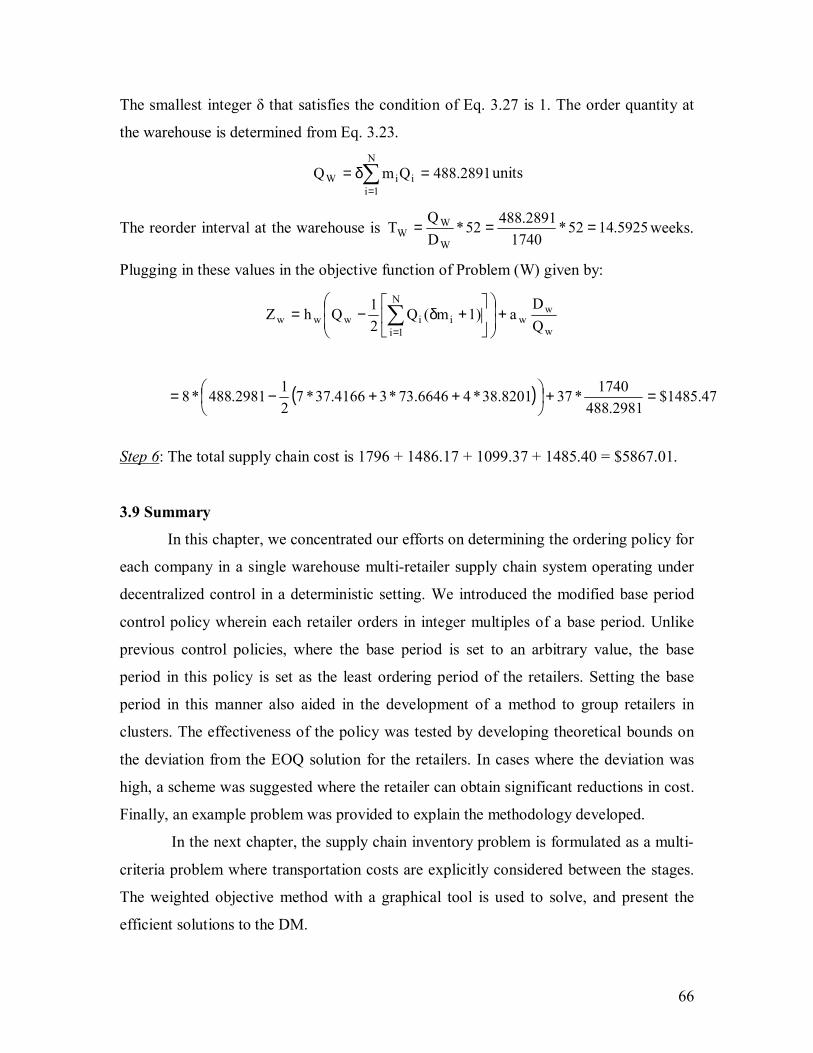
66
The smallest integer δ that satisfies the condition of Eq. 3.27 is 1. The order quantity at
the warehouse is determined from Eq. 3.23.
2891.488QmQN
1iiiW =δ= ∑
=units
The reorder interval at the warehouse is 5925.1452*1740
2891.48852*DQ
TW
WW === weeks.
Plugging in these values in the objective function of Problem (W) given by:
w
ww
N
1iiiwww Q
Da1)m(Q
21QhZ +
+δ−= ∑
=
( ) 47.1485$2981.488
1740*378201.38*46646.73*34166.37*7212981.488*8 =+
++−=
Step 6: The total supply chain cost is 1796 + 1486.17 + 1099.37 + 1485.40 = $5867.01.
3.9 Summary
In this chapter, we concentrated our efforts on determining the ordering policy for
each company in a single warehouse multi-retailer supply chain system operating under
decentralized control in a deterministic setting. We introduced the modified base period
control policy wherein each retailer orders in integer multiples of a base period. Unlike
previous control policies, where the base period is set to an arbitrary value, the base
period in this policy is set as the least ordering period of the retailers. Setting the base
period in this manner also aided in the development of a method to group retailers in
clusters. The effectiveness of the policy was tested by developing theoretical bounds on
the deviation from the EOQ solution for the retailers. In cases where the deviation was
high, a scheme was suggested where the retailer can obtain significant reductions in cost.
Finally, an example problem was provided to explain the methodology developed.
In the next chapter, the supply chain inventory problem is formulated as a multi-
criteria problem where transportation costs are explicitly considered between the stages.
The weighted objective method with a graphical tool is used to solve, and present the
efficient solutions to the DM.

67
Chapter 4
DETERMINISTIC MULTI-CRITERIA MODEL FOR A SUPPLY CHAIN WITH
TRANSPORTATION COSTS
4.1 Introduction
In the previous chapter we introduced the modified base period policy which
enabled us to determine the optimal ordering policies for each company in the supply
chain. The model assumed the availability of marginal cost information such as ordering
and holding costs. In reality, this information may not be available (as seen in Chapter 6)
or difficult to estimate, e.g., costs due to loss of goodwill when excess demand is
backordered or lost. Secondly, there are several criteria other than cost, which are often
conflicting in nature. This cannot be directly taken care of in the single objective
methodology of Chapter 3. Thirdly, for a DM to make better decisions, he/she must
choose from several solutions by evaluating tradeoff information. In a single objective
framework, the DM is provided with a single solution. Finally, the solutions generated
using a single objective methodology does not take into account the DM�s preference
information. Since the DM is an integral part of the company, it is important for the
solution to reflect his/her�s preference information.
These disadvantages can be overcome by formulating the problem as a multi-
criteria problem. In this chapter we extend the single objective cost model to a multi-
criteria model with conflicting criteria. Transportation costs are specifically included in
the model as one of the criteria.
4.2 Problem Description
The supply chain system under consideration is the same as in the previous
chapter wherein a warehouse supplies a single product to several retailers. A
manufacturer with infinite capacity replenishes the warehouse. The system operates
under a decentralized control. The inbound transportation cost at the retailer is modeled
using less than full truckload (LTL) rates while the inbound transportation cost at the
warehouse is modeled using truckload (TL) rates.
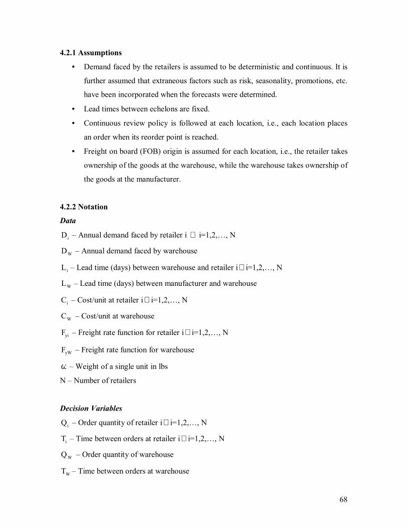
68
4.2.1 Assumptions
• Demand faced by the retailers is assumed to be deterministic and continuous. It is
further assumed that extraneous factors such as risk, seasonality, promotions, etc.
have been incorporated when the forecasts were determined.
• Lead times between echelons are fixed.
• Continuous review policy is followed at each location, i.e., each location places
an order when its reorder point is reached.
• Freight on board (FOB) origin is assumed for each location, i.e., the retailer takes
ownership of the goods at the warehouse, while the warehouse takes ownership of
the goods at the manufacturer.
4.2.2 Notation
Data
iD � Annual demand faced by retailer i ∀ i=1,2,�, N
WD � Annual demand faced by warehouse
iL � Lead time (days) between warehouse and retailer i ∀ i=1,2,�, N
WL � Lead time (days) between manufacturer and warehouse
iC � Cost/unit at retailer i ∀ i=1,2,�, N
WC � Cost/unit at warehouse
yiF � Freight rate function for retailer i ∀ i=1,2,�, N
yWF � Freight rate function for warehouse
ω � Weight of a single unit in lbs
N � Number of retailers
Decision Variables
iQ � Order quantity of retailer i ∀ i=1,2,�, N
iT � Time between orders at retailer i ∀ i=1,2,�, N
WQ � Order quantity of warehouse
WT � Time between orders at warehouse

69
ir � Reorder point for retailer i ∀ i=1,2,�, N
Wr � Reorder point for warehouse
4.3 Retailer�s Model Formulation
In a continuous review policy, the inventory at a particular location is monitored
continuously, and an order is placed when the on hand inventory reaches a reorder point
(r). The reorder point is determined as follows:
( )jTLDr −= (4.1)
where:
D- Annual demand
L � Lead time.
T � Time between orders.
j � Largest integer less than or equal to TL
When L < T (particularly when shipping using trucks), the reorder point is LD,
which is the demand during the lead time. In this case the order is placed when the on-
hand inventory reaches LD. This is shown in Fig. 4.1.
Fig. 4.1: Retailer�s Inventory Pattern
Retailer�s Criteria
The following criteria are used in the formulation of the multi-criteria problem for
all retailers:

70
• Capital invested in inventory (including in-transit inventory due to the FOB
origin).
• Number of orders placed annually.
• Annual transportation cost.
Criterion 1: Capital Invested in Inventory
The inventory at the retailer follows the saw tooth pattern shown in Fig. 4.1. The
capital invested in inventory consists of two components:
• Capital invested in inventory at retailer: It is the product of average inventory at
each retailer and the cost/unit at each retailer. The average inventory from Fig. 4.1
is Q/2. Hence, the capital invested in inventory at each retailer is simply:
ii C
2Q
i∀ (4.2)
• Annual capital invested in In-transit inventory: Since FOB origin is assumed,
each retailer is assumed to manage their inbound logistics, i.e., the retailer takes
possession of the product at the warehouse. Hence, each retailer has capital tied
up in the form of in-transit inventory. Annual capital invested in in-transit
inventory is the fraction of year the annual demand of each retailer is in transit
multiplied by the cost/unit at each retailer:
iii CD
365L
i∀ (4.3)
Thus, the capital invested in inventory is the sum of Eq. 4.2 and Eq. 4.3
iii
ii CD
365L
C2
Q+ i∀ (4.4)
Criterion 2: Number of Orders Placed Annually
The number of orders placed annually by a retailer is the ratio of annual demand
to the order quantity:
i
i
QD i∀ (4.5)

71
Criterion 3: Annual Transportation Costs
Transportation cost is an important criterion which is often overlooked in supply
chain inventory models when determining the order quantity. Shipments can be full truck
load (TL) or less than truck load (LTL). TL rates are usually stated based on distance
traveled or a fixed charge/truck while LTL rates are stated per hundredweight (CWT).
Trucking companies offer discounts on the freight rate to encourage shippers to
buy in large quantities. Since it is known that the inventory and transportation
components interact, it is essential to explicitly consider transportation costs in supply
chain models for determining the ordering policy followed by a company. There are two
problems in trying to incorporate actual freight rates:
1. Determining exact rates between every origin and destination is time consuming and
expensive.
2. The freight rate function is not differentiable.
Consider an all-units discount offered by the carrier. The cost function is:
F1Qω/100 if 0 ≤ Q < B1
F2Q ω/100 if B1 ≤ Q < B2
=)(QG .
.
FnQ ω/100 if Bn-1 ≤ Q < Bn
This function implies that if the order quantity weighs in the range [0, B1), then
the freight rate is $F1/cwt (1cwt =100lbs). Similarly, if the order quantity weighs in the
range [B1, B2), the freight rate is $F2/cwt, and so on. Also, F1>F2>�>Fn. This means that,
discounts are given by the carrier to the shipper. B1, B2,�, Bn are called the break points.
It is clear that G(Q) is not a continuous function.
An interesting feature of this function is that there would be a point in each
weight category called an indifference point beyond which the shipper pays the same rate
as that of the next weight range by over-declaring the shipment weight. This cost
function can then be converted to Fig. 4.2 by finding the indifference points in all the
weight break levels. Indifference point is the point at which the weight, when multiplied
by the actual freight rate, yields the same total cost that is charged at the next break point.

72
Fig. 4.2: Freight Rate Function
The indifference points are denoted by I1, I2,�, In in Fig. 4.2. Any shipping
weight in the interval [I1, B1) can be over-declared to B1 and charged a fixed lower rate. It
must be noted that the quantity shipped is not increased to B1, i.e., the shipper still ships
the required order quantity greater than or equal to I1, but it is declared as B1. If the
weight shipped is in the interval (B1, I2), then a variable cost ($/cwt) is charged. Fig. 4.2
is a stepwise linear function. Though the function is continuous, it is not differentiable
due to the indifference points and hence, difficult to work with analytically.
Because of these difficulties, researchers have explored the possibility of using
continuous functions to fit the actual freight rate structure. Langley (1980) was the first to
use continuous functions to model transportation costs.
Ballou (1991) suggested that freight rates should be estimated as determining
exact rates for combinations of origin-destination points for different weight breaks is
time consuming as well as expensive. He used a simple linear regression model to relate
the freight rate to the distance.
Swenseth and Godfrey (1996) used 5 different continuous functions on the actual
freight rate structure for 40 different routes. For each function the mean squared error
criterion was used to select the best function among the 40 routes. Once the best
functions were determined, they were compared with each other to find out which
function best emulates the actual freight rates. The functions that were considered were
constant, proportional, exponential, adjusted inverse and inverse functions. They

73
concluded that the inverse function exactly determines the freight rates when shipping
weights were high emulating TL rates, whereas the proportional and the adjusted inverse
functions emulated LTL rates particularly well.
Tyworth and Zeng (1998) recommend the use of a power function to model
transportation costs.
Since each retailer is going to send out trucks or use a 3PL (third party logistics
provider) to pick up the orders, the order quantity is most likely to be less than truck load
(LTL). We use the proportional function proposed by Swenseth and Godfrey (1996) as it
is easy to work with analytically. For the example problem, different continuous
functions are fit to the freight rate data to determine the function that best estimates the
transportation cost. The proportional function is very similar to a linear function proposed
by Langley (1980). Mathematically, the freight rate function by Swenseth and Godfrey
(1996) for shipping LTL for a retailer is given by:
( )yixiixiyi WWFF −α+= i∀ (4.6)
where:
Fyi- Freight rate for shipping a given load to the retailer ($/cwt)
Fxi- TL freight rate for each retailer ($/cwt)
Wxi-TL weight
Wyi- Weight shipped to each retailer i (lbs.)
αi- Rate at which freight rate increases per100lbs decrease in shipping weight for
retailer i.
Simplifying Eq. 4.6,
ωα−α+= iixiixiyi QWFF
Since Fxi and αiWxi are constants we can replace Fxi + αiWxi by another constant Ai:
ωα−= iiiyi QAF i∀ (4.7)
Eq. 4.7 is the proportional function proposed by Langley (1980), and it implies
that the freight rate decreases at a rate αi for every unit increase in Qi.
The value of αi can be determined from either Eq. 4.6 or Eq. 4.7. From Eq. 4.6, αi
is determined by minimizing the mean squared error between actual and estimated LTL
freight rates for each route. From Eq. 4.7, αi is determined by fitting a simple linear
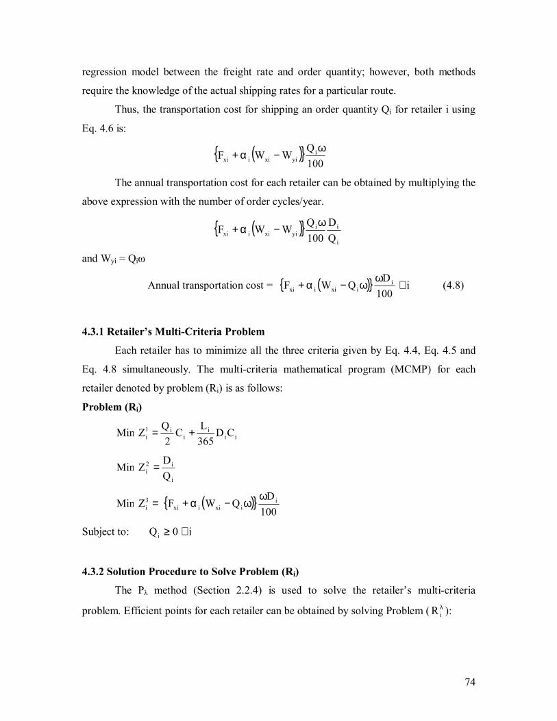
74
regression model between the freight rate and order quantity; however, both methods
require the knowledge of the actual shipping rates for a particular route.
Thus, the transportation cost for shipping an order quantity Qi for retailer i using
Eq. 4.6 is:
( ){ }100Q
WWF iyixiixi
ω−α+
The annual transportation cost for each retailer can be obtained by multiplying the
above expression with the number of order cycles/year.
( ){ }i
iiyixiixi Q
D100QWWF ω−α+
and Wyi = Qiω
Annual transportation cost = ( ){ }100
DQWF i
ixiixiω
ω−α+ i∀ (4.8)
4.3.1 Retailer�s Multi-Criteria Problem
Each retailer has to minimize all the three criteria given by Eq. 4.4, Eq. 4.5 and
Eq. 4.8 simultaneously. The multi-criteria mathematical program (MCMP) for each
retailer denoted by problem (Ri) is as follows:
Problem (Ri)
Min iii
ii1
i CD365LC
2QZ +=
Mini
i2i Q
DZ =
Min =3iZ ( ){ }
100D
QWF iixiixi
ωω−α+
Subject to: 0Qi ≥ i∀
4.3.2 Solution Procedure to Solve Problem (Ri)
The Pλ method (Section 2.2.4) is used to solve the retailer�s multi-criteria
problem. Efficient points for each retailer can be obtained by solving Problem ( λiR ):

75
Problem )( λiR
Min { }100D
QW(FQD
CD365L
C2
QZ i
ixiixi3i
i
i2iii
ii
i1ii
ωω−α+λ+λ+
+λ=λ
Subject to: 13
1k
ki =λ∑
=
0ki >λ k,i∀
0Qi ≥ i∀ kiλ - Convex combination parameter or weight assigned for criterion k for retailer i.
Every optimal solution to the λiR problem is an efficient solution to the retailer�s
multi-criteria problem. Also, all the criteria are convex, and the constraint set is a convex
set. Thus, the λiR problem is both necessary and sufficient. Hence, all the efficient points
can be generating by varying kiλ between 0 and 1.
Lemma 4.1- Objective function of Problem ( λiR ) is convex.
Proof: Taking the first and second differential of Z with respect to Q:
ωα−λ+λ−λ=λ
100D
QD
2C
dQdZ 2
ii3i2
i
i2ii
1i
i
i
3i
i2i
2i
i2
QD2
dQZd λ=
λ> 0 for positive Di, Qi and 2
iλ
■
Theorem 4.1- For each retailer, in addition to )1,0(ki ∈λ and 1
3
1k
ki =λ∑
= , the following
condition will also be satisfied by the efficient solution:
i
ii3i
1i
CD2 ωα>
λλ
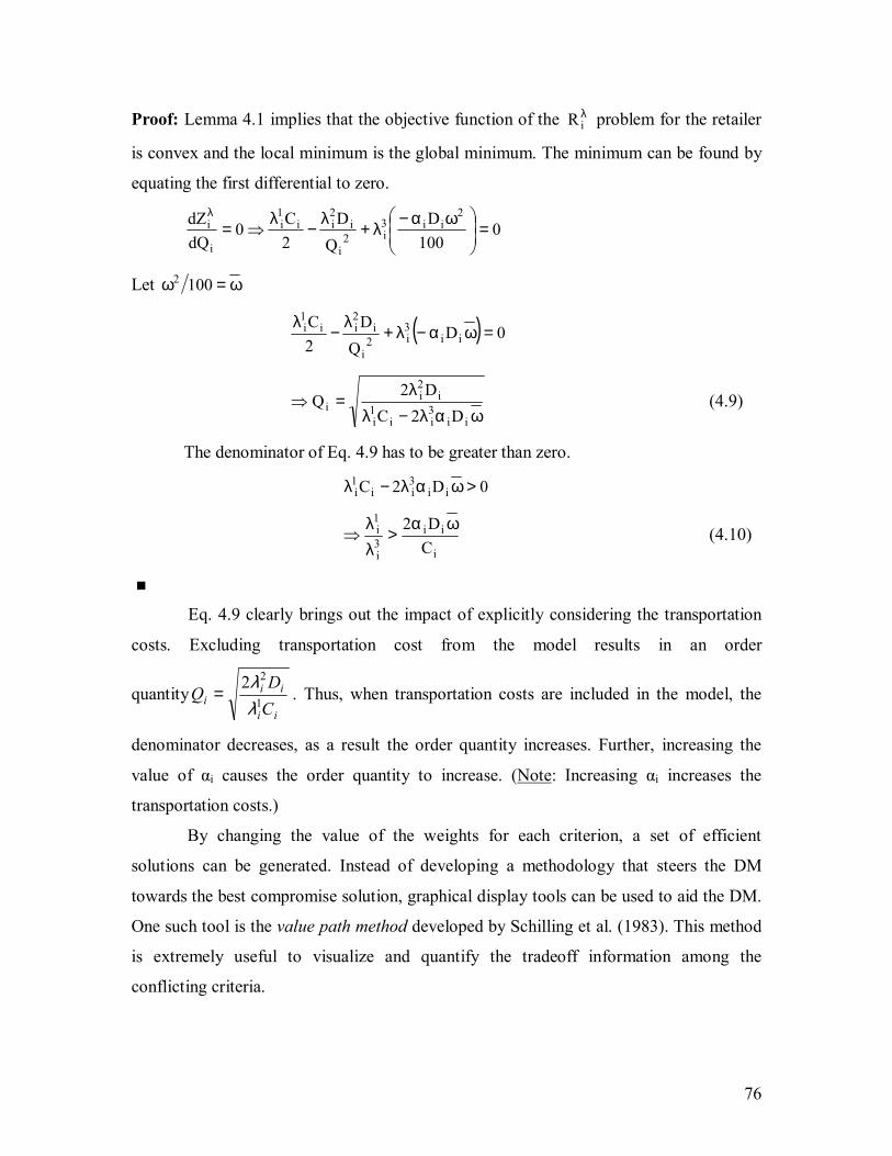
76
Proof: Lemma 4.1 implies that the objective function of the λiR problem for the retailer
is convex and the local minimum is the global minimum. The minimum can be found by
equating the first differential to zero.
0100
DQ
D2C0
dQdZ 2
ii3i2
i
i2ii
1i
i
i =
ωα−λ+λ−λ⇒=
λ
Let ω=ω 1002
( ) 0DQ
D2C
ii3i2
i
i2ii
1i =ωα−λ+λ−λ
ωαλ−λλ
=⇒ii
3ii
1i
i2i
i D2CD2
Q (4.9)
The denominator of Eq. 4.9 has to be greater than zero.
0D2C ii3ii
1i >ωαλ−λ
i
ii3i
1i
CD2 ωα>
λλ
⇒ (4.10)
■
Eq. 4.9 clearly brings out the impact of explicitly considering the transportation
costs. Excluding transportation cost from the model results in an order
quantityii
iii C
DQ 1
22λλ
= . Thus, when transportation costs are included in the model, the
denominator decreases, as a result the order quantity increases. Further, increasing the
value of αi causes the order quantity to increase. (Note: Increasing αi increases the
transportation costs.)
By changing the value of the weights for each criterion, a set of efficient
solutions can be generated. Instead of developing a methodology that steers the DM
towards the best compromise solution, graphical display tools can be used to aid the DM.
One such tool is the value path method developed by Schilling et al. (1983). This method
is extremely useful to visualize and quantify the tradeoff information among the
conflicting criteria.

77
For each alternative there is a value path. The basic premise here is that if two or
more value paths intersect each other, then all the alternatives are efficient. If the value
paths for two alternatives do not intersect, then the one lying above the other is non-
efficient. If the value path for two or more alternatives intersect then the value paths that
are above this intersection point are non-efficient.
The DM, after visually and quantitatively analyzing the tradeoff information, can
choose the best compromise solution and hence, the weight combination for each retailer.
After fixing the weight combination, each retailer can determine the time between the
orders as:
DiQ
T ii = i∀ (4.11)
4.3.3 Modified Retailer�s Problem
As in the previous chapter, the warehouse identifies the base retailer by
determining the least reorder interval among all the retailers:
iiB TMinT = (4.12)
The non-base retailers order in integer multiples of the base period:
Bii TnT = (4.13)
Substituting Eq. 4.11 into Eq. 4.13 and rewriting in terms of order quantity:
iBiB
iBii RQn
DDQnQ == (4.14)
Ri is referred to as the Demand Ratio and is defined as the ratio of demand of a
particular retailer to the demand of the retailer who orders most frequently. The
optimization problem for the base retailer, Problem λBR remains unchanged. The iR
problem for the non-base retailers is modified to incorporate Eq. 4.14 and is called
Problem (MRi).
Problem (MRi)
Min iii
ii1
i CD365LC
2QZ +=
Min i
i2i Q
DZ =

78
Min =3iZ { }
100D
QW(F iixiixi
ωω−α+
Subject to: iBii RQnQ =
0Qi ≥
1ni ≥ and integer
4.3.4 Solution Procedure to Solve Problem (MRi)
Problem (MRi) is converted to a single objective problem by using the Pλ method
as follows:
Problem )( λiMR
Min { }100D)QW(F
QDC
365LD
2QZ i
ixiixi3i
i
i2ii
iii1ii
ωω−α+λ+λ+
+λ=λ
Subject to: 13
1k
ki =λ∑
=
0ki >λ k,i∀
iBii RQnQ =
0Qi ≥
1ni ≥ and integer
Though the individual criteria are convex functions, the necessary condition of the
general Pλ problem is not satisfied since the constraint set of Problem ( )MR iλ is no
longer a convex set. Hence, all the efficient points cannot be generated. However, an
optimal solution to Problem ( )MR iλ will generate an efficient solution.
We proceed in the same way as in Lemma 3.1 and Theorem 3.1 in Chapter 3 to
determine the integer multiple, ni and hence, Qi.
Lemma 4.2- The objective function of Problem ( )λiMR is point-wise convex in ni.
Proof: For convenience, subscript �i� is eliminated.
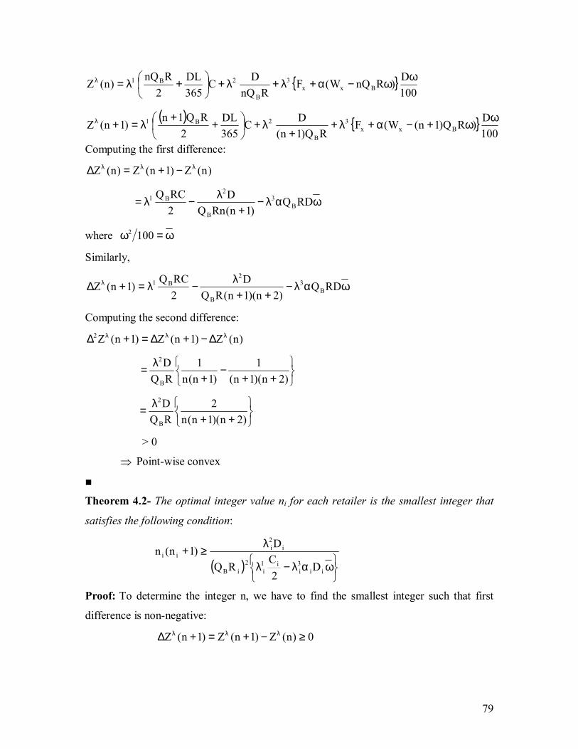
79
{ }100D)RnQW(F
RnQDC
365DL
2RnQ
)n(Z Bxx3
B
2B1 ωω−α+λ+λ+
+λ=λ
( ) { }100D)RQ)1n(W(F
RQ)1n(DC
365DL
2RQ1n
)1n(Z Bxx3
B
2B1 ωω+−α+λ++
λ+
+
+λ=+λ
Computing the first difference:
)n(Z)1n(Z)n(Z λλλ −+=∆
ωαλ−+
λ−λ= RDQ)1n(RnQ
D2RCQ
B3
B
2B1
where ω=ω 1002
Similarly,
ωαλ−++
λ−λ=+∆ λ RDQ)2n)(1n(RQ
D2RCQ
)1n(Z B3
B
2B1
Computing the second difference:
)n(Z)1n(Z)1n(Z2 λλλ ∆−+∆=+∆
++−
+λ=
)2n)(1n(1
)1n(n1
RQD
B
2
++λ=
)2n)(1n(n2
RQD
B
2
> 0
⇒ Point-wise convex
■
Theorem 4.2- The optimal integer value ni for each retailer is the smallest integer that
satisfies the following condition:
( )
ωαλ−λ
λ≥+
ii3i
i1i
2iB
i2i
ii
D2
CRQ
D)1n(n
Proof: To determine the integer n, we have to find the smallest integer such that first
difference is non-negative:
0)n(Z)1n(Z)1n(Z ≥−+=+∆ λλλ

80
0RDQ)1n(RnQ
D2RCQ
B3
B
2B1 ≥ωαλ−
+λ−λ⇒
ωαλ−λ≤+
λ⇒ RDQ
2RCQ
)1n(RnQD
B3B1
B
2
( )
ωαλ−λ
λ≥+⇒D
2CRQ
D)1n(n312
B
2
(4.15)
■
As in Eq. 4.9, we can bring the importance of including transportation costs in the
model formulation by observing Eq. 4.15. If transportation costs were not included, then
Eq. 4.15 simplifies to:
( )
λ
λ≥+
2CRQ
D)1n(n12
B
2
(4.16)
Clearly, the denominator of Eq. 4.15 is less than the denominator of Eq. 4.16. As a result,
the integer multiple �n� could be rounded off to a larger integer, which in turn will
increase the order quantity.
4.4 Warehouse�s Model Formulation
Being a decentralized system, the warehouse will use the ordering information of
the retailers to formulate its multi-criteria mathematical programming (MCMP) problem.
For the warehouse to formulate its MCMP, it has to first determine the average inventory.
This expression** is given by:
+δ− ∑=
N
1iiiW 1)m(Q
21Q
imδ is the total number of orders placed by retailer i during the reorder interval of the
warehouse. The mi�s refer to the number of orders placed by retailer i during the smallest
reorder interval of the warehouse given by BN21N21 T)n,...,n,n(M.C.L)T,...,T,T(M.C.L = .
** For a detailed explanation of how this expression was derived please refer to Section 3.5.1.
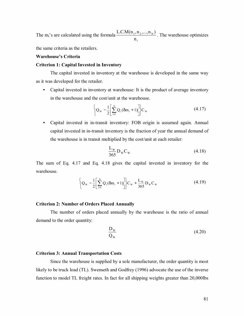
81
The mi�s are calculated using the formulai
N21
n)n,...,n,n(M.C.L
. The warehouse optimizes
the same criteria as the retailers.
Warehouse�s Criteria
Criterion 1: Capital Invested in Inventory
The capital invested in inventory at the warehouse is developed in the same way
as it was developed for the retailer.
• Capital invested in inventory at warehouse: It is the product of average inventory
in the warehouse and the cost/unit at the warehouse.
W
N
1iiiW C1)m(Q
21Q
+δ− ∑=
(4.17)
• Capital invested in in-transit inventory: FOB origin is assumed again. Annual
capital invested in in-transit inventory is the fraction of year the annual demand of
the warehouse is in transit multiplied by the cost/unit at each retailer:
WWW CD
365L
(4.18)
The sum of Eq. 4.17 and Eq. 4.18 gives the capital invested in inventory for the
warehouse.
WWW
W
N
1iiiW CD
365L
C1)m(Q21Q +
+δ− ∑=
(4.19)
Criterion 2: Number of Orders Placed Annually
The number of orders placed annually by the warehouse is the ratio of annual
demand to the order quantity:
W
W
QD (4.20)
Criterion 3: Annual Transportation Costs
Since the warehouse is supplied by a sole manufacturer, the order quantity is most
likely to be truck load (TL). Swenseth and Godfrey (1996) advocate the use of the inverse
function to model TL freight rates. In fact for all shipping weights greater than 20,000lbs
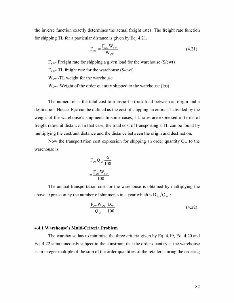
82
the inverse function exactly determines the actual freight rates. The freight rate function
for shipping TL for a particular distance is given by Eq. 4.21.
yW
xWxWyW W
WFF = (4.21)
FyW- Freight rate for shipping a given load for the warehouse ($/cwt)
FxW- TL freight rate for the warehouse ($/cwt)
WxW -TL weight for the warehouse
WyW- Weight of the order quantity shipped to the warehouse (lbs)
The numerator is the total cost to transport a truck load between an origin and a
destination. Hence, FyW can be defined as the cost of shipping an entire TL divided by the
weight of the warehouse�s shipment. In some cases, TL rates are expressed in terms of
freight rate/unit distance. In that case, the total cost of transporting a TL can be found by
multiplying the cost/unit distance and the distance between the origin and destination.
Now the transportation cost expression for shipping an order quantity QW to the
warehouse is:
100
QF WyWω
=100
WF xWxW
The annual transportation cost for the warehouse is obtained by multiplying the
above expression by the number of shipments in a year which is WW QD :
100D
QWF W
W
xWxW (4.22)
4.4.1 Warehouse�s Multi-Criteria Problem
The warehouse has to minimize the three criteria given by Eq. 4.19, Eq. 4.20 and
Eq. 4.22 simultaneously subject to the constraint that the order quantity at the warehouse
is an integer multiple of the sum of the order quantities of the retailers during the ordering

83
period of the warehouse��. The multi-criteria nonlinear integer program for the warehouse
denoted by Problem (W) is as follows:
Problem (W)
Min WWW
W
N
1iiiW
1W CD
365L
C1)m(Q21QZ +
+δ−= ∑=
Min W
W2W Q
DZ =
Min 100D
QWF
Z W
W
xWxW3W =
Subject to: ∑=
δ=N
1iiiW QmQ
0QW ≥
1≥δ and integer
4.4.2 Solution Procedure to Solve Problem (W)
The Pλ method is again used to convert Problem (W) to a single objective math
program:
Problem (Wλ)
100D
QWF
QD
CD365L
C1)m(Q21QZMin W
W
xWxW3W
W
W2WWW
WW
N
1iiiW
1WW λ+λ+
+
+δ−λ= ∑=
λ
Subject to: 13
1k
kW =λ∑
=
0kW >λ k∀
∑=
δ=N
1iiiW QmQ
0QW ≥
1≥δ and integer kWλ - Convex combination parameter or weight assigned for criterion k for the warehouse.
�� For details please see Section 3.5.1.

84
As in Problem ( )MR iλ , the feasible region is no longer a convex set; hence, the
necessary condition of the general Pλ problem is not satisfied, and all the efficient points
cannot be generated. However, an optimal solution to Problem (Wλ) will generate an
efficient solution.
The order quantity of the warehouse can be determined once the value of the
integer multiple δ is determined. To determine δ, we have to prove that the objective
function of Problem (Wλ) is point-wise convex.
Lemma 4.3- The objective function of Problem (Wλ) is point-wise convex in δ.
Proof: Writing the objective function in terms of δ:
100D
Qm
WF
Qm
DC
365DL
QQm2
)(Z WN
1iii
xWxW3WN
1iii
W2WW
N
1i
WWi
N
1iii
1W
W
∑∑∑∑
==
==
λ
δλ+
δλ+
+−δ
λ=δ
100D
Qm)1(
WF
Qm)1(
DC
365DL
QQm)1(2
)1(Z WN
1iii
xWxW3WN
1iii
W2WW
N
1i
WWi
N
1iii
1W
W
∑∑∑∑
==
==
λ
+δλ+
+δλ+
+−+δ
λ=+δ
)(Z)1(Z)(Z WWW δ−+δ=δ∆ λλλ
( ) ( ) 100
D
1Qm
WF
1Qm
DCQm
2W
N
1iii
xWxW3W
i
N
1ii
W2W
Wi
N
1ii
1W
+δδ
λ
−+δδ
λ
−
λ=
∑∑∑
==
=
Similarly,
( )( ) ( )( ) 100D
21Qm
WF
21Qm
DCQm
2)1(Z W
N
1iii
xWxW3W
i
N
1ii
W2W
Wi
N
1ii
1W
W
+δ+δ
λ
−+δ+δ
λ
−
λ=+δ∆
∑∑∑
==
=
λ
Computing the second difference:
)(Z)1(Z)1(Z WWW2 δ∆−+δ∆=+δ∆ λλλ
( )( ) ( )( ) ( )( ) ( )( ) 100D
211
11
Qm
WF21
11
1
Qm
D WN
1iii
xWxW3W
i
N
1ii
W2W
+δ+δ−
+δδ
λ
+
+δ+δ−
+δδ
λ
=
∑∑==
( )( )( )21Qm
2100D
WFDN
1iii
WxWxW
3WW
2W
+δ+δδ
λ+λ=
∑=

85
> 0
⇒ Point-wise convex
■
Theorem 4.3- The optimal integer value δ for the warehouse is the smallest integer that
satisfies the following condition:
λ
+λ
λ
≥+δδ
∑
∑
=
=
100WF
CQm
D2)1( xWxW
3W2
W
W1W
2
i
N
1ii
N
1ii
Proof: The integer δ can be found by finding the smallest integer such that the first
difference is non-negative i.e.
0)m(Z)1m(Z)1m(Z WWW ≥−+=+∆ λλλ
( ) ( )0
100D
1Qm
WF
1Qm
DCQm
2W
N
1iii
xWxW3W
i
N
1ii
W2W
Wi
N
1ii
1W ≥
+δδ
λ
−+δδ
λ
−
λ⇒
∑∑∑
==
=
( )
λ
+λ+δδ
≥
λ⇒
∑∑
=
= 100WF
1Qm
DCQm
2xWxW
3W2
W
i
N
1ii
WWi
N
1ii
1W
λ
+λ
λ
≥+δδ⇒
∑
∑
=
=
100WF
CQm
D2)1( xWxW
3W2
W
W1W
2
i
N
1ii
N
1ii
(4.23)
■
Again, observing Eq. 4.23 we can analyze the importance of including
transportation costs in the model formulation. If criterion 3 (transportation cost) was not
included in the model formulation, Eq. 4.23 becomes:
W1W
2
i
N
1ii
N
1ii
2W
CQm
D2)1(
λ
λ≥+δδ
∑
∑
=
= (4.24)
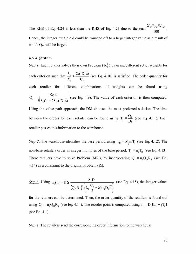
86
The RHS of Eq. 4.24 is less than the RHS of Eq. 4.23 due to the term100
WF xWxW3Wλ
.
Hence, the integer multiple δ could be rounded off to a larger integer value as a result of
which QW will be larger.
4.5 Algorithm
Step 1: Each retailer solves their own Problem ( λiR ) by using different set of weights for
each criterion such that i
ii3i
1i
CD2 ωα
>λλ (see Eq. 4.10) is satisfied. The order quantity for
each retailer for different combinations of weights can be found using
ωαλ−λλ
=ii
3ii
1i
i2i
i D2CD2
Q (see Eq. 4.9). The value of each criterion is then computed.
Using the value path approach, the DM chooses the most preferred solution. The time
between the orders for each retailer can be found using DiQ
T ii = (see Eq. 4.11). Each
retailer passes this information to the warehouse.
Step 2: The warehouse identifies the base period using iiB TMinT = (see Eq. 4.12). The
non-base retailers order in integer multiples of the base period, Bii TnT = (see Eq. 4.13).
These retailers have to solve Problem (MRi), by incorporating iBii RQnQ = (see Eq.
4.14) as a constraint to the original Problem (Ri).
Step 3: Using ( )
ωαλ−λ
λ≥+
ii3i
i1i
2iB
i2i
ii
D2
CRQ
D)1n(n (see Eq. 4.15), the integer values
for the retailers can be determined. Then, the order quantity of the retailers is found out
using iBii RQnQ = (see Eq. 4.14). The reorder point is computed using ( )iiii jTLDr −=
(see Eq. 4.1).
Step 4: The retailers send the corresponding order information to the warehouse.

87
Step 5: The warehouse uses this information to formulate its own MCMP (Problem (W))
and determines its integer multiple given by
λ
+λ
λ
≥+δδ
∑
∑
=
=
100WF
CQm
D2)1( xWxW
3W2
W
W1W
2
i
N
1ii
N
1ii
(see Eq. 4.23) and hence its order
quantity for different weight combinations. Using the value path approach, the DM can
choose the most preferred solution.
Note 1: A heuristic procedure to determine the number of trucks needed for each
location, particularly for the warehouse is as follows. If a location orders Qω lbs every
cycle and the maximum allowable weight is Wx lbs, then the number of trucks needed
is
xWQω . If the number of TL is
xWQω and the weight shipped in the
th
xWQ
ω truck is less
than the weight requirement for a TL, then the firm is charged a fixed TL rate/ full truck
and a LTL rate for the th
xWQ
ω truck.
Note 2: We made an important assumption regarding the type of shipments used by the
retailers and the warehouse, and hence the type of freight rate function used. For the
retailers, a proportional function was used to model the transportation costs since it was
assumed that shipments are LTL. For the warehouse, an inverse function was used since
it was assumed to use TL shipments. If, after solving the retailer�s problem the weight of
the order quantity is such that it can be declared as a TL, then the annual transportation
cost might be overestimated. Similarly, if the warehouse�s shipment weight is not large
enough to be declared as a TL, then the annual transportation cost is overestimated at the
warehouse. This difficulty can be overcome in three ways:
1) Recalculate the annual transportation costs by plugging in the weight shipped in
the appropriate freight rate function, i.e., for the retailers use the inverse function
and for the warehouse use the proportional function.

88
2) Resolve the MCMP with the appropriate freight rate function, i.e., use the inverse
function in Problem (Ri) and the proportional function in Problem (W).
3) Formulate the MCMP with an additional binary variable which will indicate when
to use the proportional function and when to use the inverse function. This
formulation is described in the next section.
4.6 General MCMP for Retailer and Warehouse
As noted in the previous section, the assumption that the retailers use LTL and the
warehouse uses TL can be relaxed by introducing a binary variable which is activated
when the weight shipped is less than the indifference point needed to declare the load as a
TL, i.e.,
1IQ =γ⇒<ω (4.25)
and 0IQ =γ⇒≥ω (4.26)
Qω � Weight shipped
I- Weight beyond which the shipment is declared as TL (Indifference point).
)1,0(∈γ and integer
Either Eq. 4.25 or Eq. 4.26 can occur but not both. This can be modeled as:
)1(M)I(Q γ−≤ε−−ω (4.27)
γ≤+ω− MIQ (4.28)
M- Very large number
ε - Infinitesimally small value
To see how constraints Eq. 4.25 and Eq. 4.26 represent Eq. 4.27 and Eq. 4.28, we
consider two cases:
Case 1: IQ ≥ω
0IQIQ ≥−ω⇒≥ω . The LHS of Eq. 4.28 is negative. Eq. 4.28 is satisfied when 0=γ or
1=γ , but Eq. 4.27 is infeasible when 1=γ . This means that γ is forced to 0. Hence, Eq.
4.26 ≡ Eq. 4.28. When 0=γ , Eq. 4.27 is redundant.
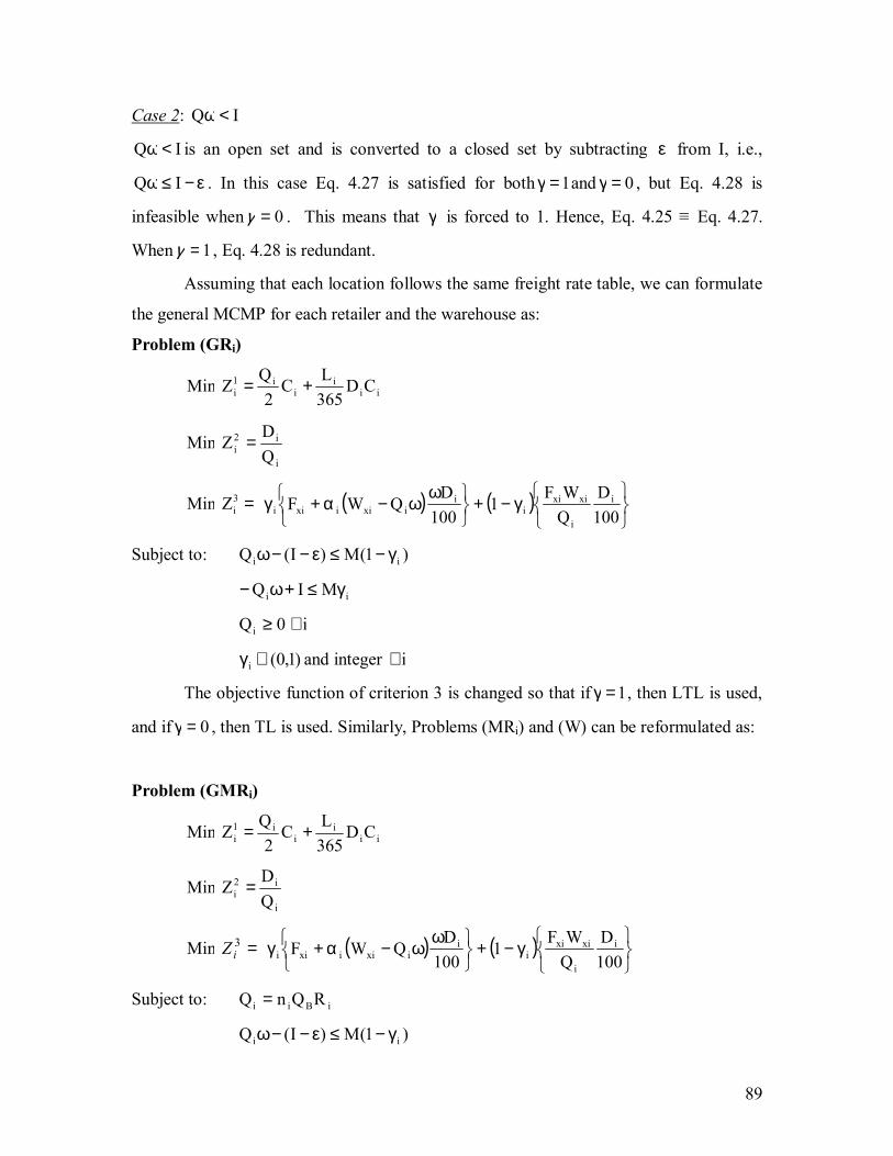
89
Case 2: IQ <ω
IQ <ω is an open set and is converted to a closed set by subtracting ε from I, i.e.,
ε−≤ω IQ . In this case Eq. 4.27 is satisfied for both 1=γ and 0=γ , but Eq. 4.28 is
infeasible when 0=γ . This means that γ is forced to 1. Hence, Eq. 4.25 ≡ Eq. 4.27.
When 1=γ , Eq. 4.28 is redundant.
Assuming that each location follows the same freight rate table, we can formulate
the general MCMP for each retailer and the warehouse as:
Problem (GRi)
Min iii
ii1
i CD365LC
2QZ +=
Mini
i2i Q
DZ =
Min =3iZ ( ) ( )
γ−+
ω
ω−α+γ100D
QWF
1100
DQWF i
i
xixii
iixiixii
Subject to: )1(M)I(Q ii γ−≤ε−−ω
ii MIQ γ≤+ω−
0Qi ≥ i∀ )1,0(i ∈γ and integer i∀
The objective function of criterion 3 is changed so that if 1=γ , then LTL is used,
and if 0=γ , then TL is used. Similarly, Problems (MRi) and (W) can be reformulated as:
Problem (GMRi)
Min iii
ii1
i CD365LC
2QZ +=
Mini
i2i Q
DZ =
Min =3iZ ( ) ( )
γ−+
ω
ω−α+γ100D
QWF
1100
DQWF i
i
xixii
iixiixii
Subject to: iBii RQnQ =
)1(M)I(Q ii γ−≤ε−−ω
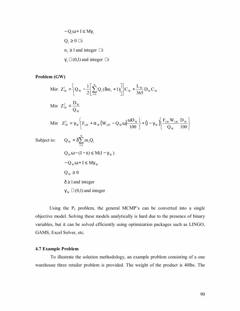
90
ii MIQ γ≤+ω−
0Qi ≥ i∀ 1ni ≥ and integer i∀
)1,0(i ∈γ and integer i∀
Problem (GW)
Min WWW
W
N
1iiiW
1W CD
365L
C1)m(Q21QZ +
+δ−= ∑=
Min W
W2W Q
DZ =
Min ( ) ( )
γ−+
ω
ω−α+γ=100D
QWF
1100D
QWFZ W
W
xWxWW
WWxWWxWW
3W
Subject to: ∑=
δ=N
1iiiW QmQ
)1(M)I(Q WW γ−≤ε−−ω
WW MIQ γ≤+ω−
0QW ≥
1≥δ and integer
)1,0(W ∈γ and integer
Using the Pλ problem, the general MCMP�s can be converted into a single
objective model. Solving these models analytically is hard due to the presence of binary
variables, but it can be solved efficiently using optimization packages such as LINGO,
GAMS, Excel Solver, etc.
4.7 Example Problem
To illustrate the solution methodology, an example problem consisting of a one
warehouse three retailer problem is provided. The weight of the product is 40lbs. The

91
cost, demand (same as in Chapter 3), and lead time data for each retailer and the
warehouse is given in Table 4.1.
Table 4.1: Data for Example Problem
Demand (Di) Cost (Ci) Lead Time (Li) Retailer 1 800 units $100 5 days Retailer 2 525 units $140 4 days Retailer 3 415 units $150 3 days
Warehouse 1740 units $65 10 days
The freight rate data is taken from Swenseth and Godfrey (2001) and is
reproduced as Table 4.2.
Table 4.2: Freight Rate Data
Weight Break (lbs) Rate Minimum Charge $40.00
1-499 $17.60/cwt 500-999 $14.80/cwt
1000-1999 $13.80/cwt 2000-4999 $12.80/cwt 5000-9999 $12.40/cwt
10000-19999 $6.08/cwt ≥ 20000 (Truckload) $1110.00
The freight rate data with indifference points is shown in Table 4.3.
Table 4.3: Freight Rate Data with Indifference Points
Weight Break (lbs) Rate ≤ 227 $40.00
228-420 $17.60/cwt 421-499 $74.00 500-932 $14.80/cwt 933-999 $138.00
1000-1855 $13.80/cwt 1856-1999 $256.00 2000-4749 $12.80/cwt 4750-9999 $608.00
10000-18256 $6.08/cwt ≥ 18257 $1110.00

92
If the weight shipped, e.g., is 5000 lbs, then the shipment is over-declared to
10000 lbs and the company is charged a fixed rate of $608. The effective rate (Warsing,
2006) for this shipment is 608/5000 is $0.1216/lb or $12.16/cwt. If the weight of the
shipment exceeds 18256 lbs, it is declared as a TL.
Instead of using the proportional function we decided to fit different functions to
the effective rates obtained from Table 4.3. The function which has the maximum R2
value is selected as the best function to estimate the freight rates. A summary of the
different functions used and their R2 value are given in Table 4.4.
Table 4.4: Summary of Curve Fitting
Function type Function R2 value Linear -0.0487x + 17.25 0.2164
Quadratic 0.0002x2 - 0.134x + 19.302 0.2929 Cubic -1E-06x3 + 0.0011x2 - 0.2457x + 20.783 0.3294 Power 32.686x-0.3484 0.8798
Exponential 16.137e-0.005x 0.74 Logarithmic -4.8782Ln(x) + 28.596 0.5399
From Table 4.4, we can see that the power function provides the best estimate of
the LTL rate. In fact, the linear function provides the worst fit. It is assumed that the
freight rates are same for all the retailers. The results of Problem (Ri) and Problem (MRi)
were derived based on the assumption that the transportation cost was of the linear type
and hence cannot be used. Re-deriving the expressions using the power function leads to
mathematically intractable expressions for the order quantity. However, the general
power function a(x)b is a convex function provided b is negative. Hence, the objective
function of Problem ( λiR ) (Problem ( λ
iMR )) is convex (point-wise convex). Standard
optimization packages like Excel Solver or Lingo can be used to solve for the ordering
policy.
Table 4.5 provides the upper and lower bounds for the order quantity set by the
DM of each retailer.

93
Table 4.5: Bounds on Order Quantity
Upper bound Lower bound Retailer 1 100 20 Retailer 2 80 15 Retailer 3 70 10
A sample MCMP for Retailer 1 is given as:
Problem (R1)
)100)(800(365
51002
QZMin 11
1 +=
1
21 Q
800ZMin =
( )100
)40)(800(100Q686.32ZMin 3484.01
31
−ω=
Subject to: 20Q1 ≥
100Q1 ≤
To prevent one criterion from dominating the other, normalization must be done.
Normalization is done by dividing the weight assigned to a particular criterion by the
ideal value of that criterion. Ideal value of each criterion is found by minimizing the
individual criterion independently subjected to the upper and lower bound constraints.
This is the same as assigning unit weight to a criterion and 0 to the others. The ideal
values for the criteria are $2095.89, 8, and $3436.67. The next step is to convert the
original MCMP to a single objective type by using the Pλ method as shown for Retailer 1:
Problem( λ1R )
( )( )
( )100
)40)(800(100Q686.3267.3436
Q800
8100800
3655100
2Q
89.2095ZMin
3484.01
31
1
211
11
1
−
λ
ωλ
+
λ+
+
λ=
Subject to: 20Q1 ≥
100Q1 ≤
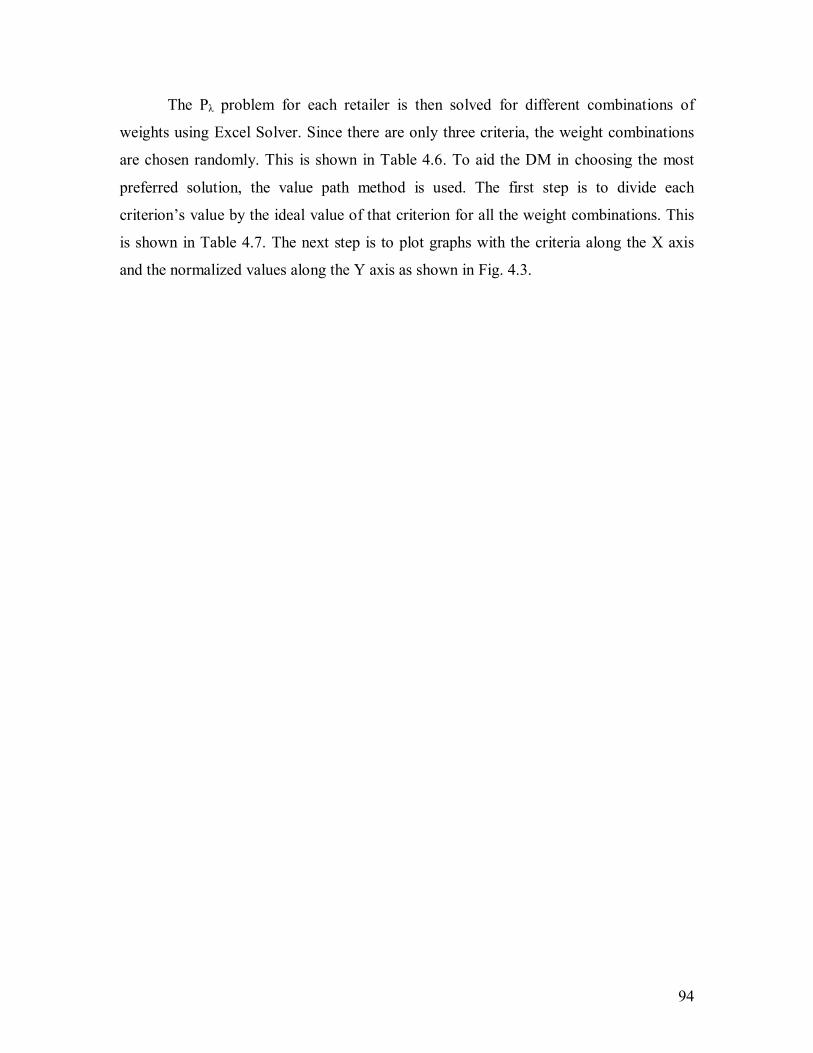
94
The Pλ problem for each retailer is then solved for different combinations of
weights using Excel Solver. Since there are only three criteria, the weight combinations
are chosen randomly. This is shown in Table 4.6. To aid the DM in choosing the most
preferred solution, the value path method is used. The first step is to divide each
criterion�s value by the ideal value of that criterion for all the weight combinations. This
is shown in Table 4.7. The next step is to plot graphs with the criteria along the X axis
and the normalized values along the Y axis as shown in Fig. 4.3.
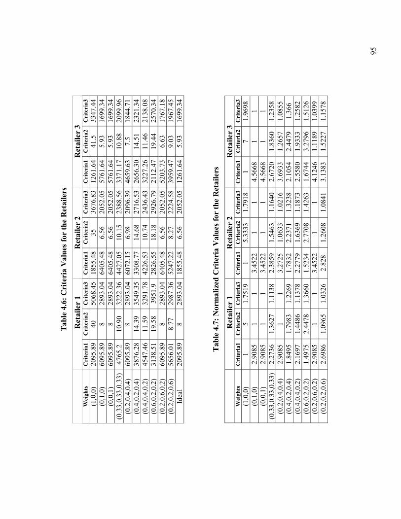
95
Tab
le 4
.6: C
rite
ria
Val
ues
for
the
Ret
aile
rs
R
etai
ler
1 R
etai
ler
2 R
etai
ler
3
Wei
ghts
C
rite
ria1
C
rite
ria2
C
rite
ria3
C
rite
ria1
C
rite
ria2
C
rite
ria3
C
rite
ria1
C
rite
ria2
C
rite
ria3
(1
,0,0
) 20
95.8
940
50
68.4
518
55.4
835
36
76.8
312
61.6
441
.5
3347
.44
(0,1
,0)
6095
.89
8 28
93.0
464
05.4
86.
56
2052
.05
5761
.64
5.93
16
99.3
4 (0
,0,1
) 60
95.8
98
2893
.04
6405
.48
6.56
20
52.0
557
61.6
45.
93
1699
.34
(0.3
3,0.
33,0
.33)
47
65.2
10
.90
3222
.36
4427
.05
10.1
5 23
88.5
633
71.1
710
.88
2099
.96
(0.2
,0.4
,0.4
) 60
95.8
98
2893
.04
6072
.15
6.98
20
96.3
946
59.6
37.
5 18
44.7
1 (0
.4,0
.2,0
.4)
3876
.28
14.3
9 35
49.3
533
08.7
714
.68
2716
.53
2656
.30
14.5
1 23
21.3
4 (0
.4,0
.4,0
.2)
4547
.46
11.5
9 32
91.7
842
26.5
310
.74
2436
.43
3227
.26
11.4
6 21
38.0
8 (0
.6,0
.2,0
.2)
3138
.51
19.5
8 39
51.9
28
26.5
518
.18
2926
.79
2112
.47
19.4
4 25
70.3
4 (0
.2,0
.6,0
.2)
6095
.89
8 28
93.0
464
05.4
86.
56
2052
.05
5203
.73
6.63
17
67.1
8 (0
.2,0
.2,0
.6)
5656
.01
8.77
29
87.3
652
47.2
28.
27
2224
.58
3959
.47
9.03
19
67.4
5 Id
eal
2095
.89
8 28
93.0
418
55.4
86.
56
2052
.05
1261
.64
5.93
16
99.3
4
Tab
le 4
.7: N
orm
aliz
ed C
rite
ria
Val
ues f
or th
e R
etai
lers
R
etai
ler
1 R
etai
ler
2 R
etai
ler
3 W
eigh
ts
Cri
teri
a1
Cri
teri
a2
Cri
teri
a3
Cri
teri
a1
Cri
teri
a2
Cri
teri
a3
Cri
teri
a1
Cri
teri
a2
Cri
teri
a3
(1,0
,0)
1 5
1.75
19
1 5.
3333
1.
7918
1
7 1.
9698
(0
,1,0
) 2.
9085
1
1 3.
4522
1
1 4.
5668
1
1 (0
,0,1
) 2.
9085
1
1 3.
4522
1
1 4.
5668
1
1 (0
.33,
0.33
,0.3
3)
2.27
36
1.36
27
1.11
38
2.38
59
1.54
63
1.16
40
2.67
20
1.83
60
1.23
58
(0.2
,0.4
,0.4
) 2.
9085
1
1 3.
2725
1.
0633
1.
0216
3.
6933
1.
2657
1.
0855
(0
.4,0
.2,0
.4)
1.84
95
1.79
83
1.22
69
1.78
32
2.23
71
1.32
38
2.10
54
2.44
79
1.36
6 (0
.4,0
.4,0
.2)
2.16
97
1.44
86
1.13
78
2.27
79
1.63
69
1.18
73
2.55
80
1.93
33
1.25
82
(0.6
,0.2
,0.2
) 1.
4975
2.
4478
1.
3660
1.
5234
2.
7708
1.
4263
1.
6744
3.
2796
1.
5126
(0
.2,0
.6,0
.2)
2.90
85
1 1
3.45
22
1 1
4.12
46
1.11
89
1.03
99
(0.2
,0.2
,0.6
) 2.
6986
1.
0965
1.
0326
2.
828
1.26
08
1.08
41
3.13
83
1.52
27
1.15
78

96

97
Fig. 4.3: Value Path Graphs for Retailers
In Fig. 4.3 all the value paths intersect, which implies that all the alternatives
belong to the efficient set. The DM by looking at Fig. 4.3 can visualize how each
criterion varies with different weight combinations. Further, by looking at Table 4.7, the
DM can quantify the tradeoff information among different weight combinations. For
example, if the DM for Retailer 1 wants to switch from weight combination (1, 0, 0) to
weight combination (0.4, 0.2, 0.4), he/she is willing to increase the capital invested in
inventory by 84.95% from the ideal value in order to decrease the annual number of
orders and annual transportation cost by 64.03% and 29.96%, respectively. This result
intuititively makes sense as the DM�s preference for the capital invested in inventory
criterion has reduced, while his/her�s preference towards number of orders, and annual
transportation costs has increased. Thus, a tradeoff analysis can be used to validate the
results by observing the critieria values, and verifying if their variations make sense.
This method is a simple way of incorporating the DM�s preference information.
The DM is involved entirely during the decision making process. Also, the cognitive
burden on the DM is less. If the DM is not satisfied with the efficient solutions, then
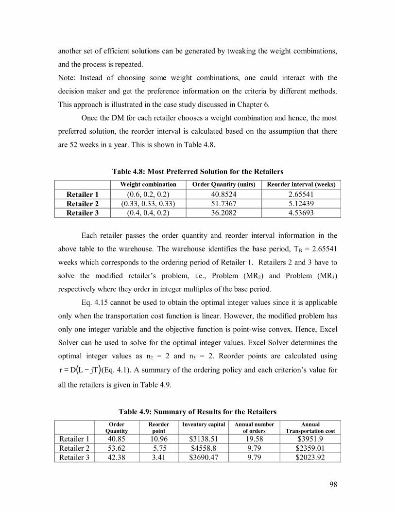
98
another set of efficient solutions can be generated by tweaking the weight combinations,
and the process is repeated.
Note: Instead of choosing some weight combinations, one could interact with the
decision maker and get the preference information on the criteria by different methods.
This approach is illustrated in the case study discussed in Chapter 6.
Once the DM for each retailer chooses a weight combination and hence, the most
preferred solution, the reorder interval is calculated based on the assumption that there
are 52 weeks in a year. This is shown in Table 4.8.
Table 4.8: Most Preferred Solution for the Retailers
Weight combination Order Quantity (units) Reorder interval (weeks) Retailer 1 (0.6, 0.2, 0.2) 40.8524 2.65541 Retailer 2 (0.33, 0.33, 0.33) 51.7367 5.12439 Retailer 3 (0.4, 0.4, 0.2) 36.2082 4.53693
Each retailer passes the order quantity and reorder interval information in the
above table to the warehouse. The warehouse identifies the base period, TB = 2.65541
weeks which corresponds to the ordering period of Retailer 1. Retailers 2 and 3 have to
solve the modified retailer�s problem, i.e., Problem (MR2) and Problem (MR3)
respectively where they order in integer multiples of the base period.
Eq. 4.15 cannot be used to obtain the optimal integer values since it is applicable
only when the transportation cost function is linear. However, the modified problem has
only one integer variable and the objective function is point-wise convex. Hence, Excel
Solver can be used to solve for the optimal integer values. Excel Solver determines the
optimal integer values as n2 = 2 and n3 = 2. Reorder points are calculated using
( )jTLDr −= (Eq. 4.1). A summary of the ordering policy and each criterion�s value for
all the retailers is given in Table 4.9.
Table 4.9: Summary of Results for the Retailers
Order Quantity
Reorder point
Inventory capital Annual number of orders
Annual Transportation cost
Retailer 1 40.85 10.96 $3138.51 19.58 $3951.9 Retailer 2 53.62 5.75 $4558.8 9.79 $2359.01 Retailer 3 42.38 3.41 $3690.47 9.79 $2023.92

99
The output of the retailers is used to formulate the warehouse�s problem. The
annual demand faced by the warehouse is the sum of the annual demands faced by all the
retailers and is 1740 units. The lead time and cost at the warehouse are 10 days and $65,
respectively. Assuming a truck can carry up to 46,000lbs (460 cwt), TL rate is 1110/460
= $2.413/cwt.
The number of orders that each retailer places during the smallest ordering period
of the warehouse is found by:
1)2,2,1(M.C.Lm1 = =2
Similarly, m2 = 1 and m3 = 1. The MCMP for the warehouse for the example is given as:
[ ] )65)(1740(3651065)1(38.42)1(62.53)12(85.40
21QZMin W
1W +
+δ++δ++δ−=
W
2W Q
1740ZMin =
W
3W Q100
)1740)(46000)(413.2(ZMin =
Subject to: δ= 71.177QW
0QW ≥
1≥δ and integer
As in the retailer problem normalization is done by dividing the weight of a
criterion by the ideal value of that criterion. The ideal value is determined by optimizing
the individual criterion subjected to upper bound and lower bound constraints on either
QW or δ, in addition to the original constraints of Problem (Wλ). The upper and lower
bound used for δ is [1,5]. The ideal values are $4426.33, 1.96 and $2173.68. This
formulation is converted to a single objective problem by using the Pλ method and is
given as:
[ ]
W
W3
W
W2
W
W1
W
Q100)1740)(46000)(413.2(
68.2173Q1740
96.1
)65)(1740(3651065)1(38.42)1(62.53)12(85.40
21Q
33.4426ZMin
λ+
λ+
+
+δ++δ++δ−
λ=λ

100
Subject to: δ= 71.177QW
0QW ≥
1≥δ
5≤δ
δ - integer
The ordering policy of the warehouse can be directly determined by computing
the RHS of Eq. 4.23,
λ
+λ
λ
≥+δδ
∑
∑
=
=
100WF
CQm
D2)1( xWxW
3W2
W
W1W
2
i
N
1ii
N
1ii
, for different
weight combinations. Note that Eq. 4.23 cannot be used to determine the ordering
policies for the weight combinations (1,0,0), (0,1,0) and (0,0,1). By changing the weight
parameters, different values of δ can be obtained. The DM can then use the value path
approach explained previously to choose the most preferred solution. The δ calculation
for the weight combination (0.6,0.2,0.2) using the RHS of Eq. 4.23 is given as:
25534.2100
)46000)(413.2()68.21732.0(96.12.065*)33.44266.0(*)71.177(
)1740(22 =δ⇒=
+
The values of the decision variables for the different weight combinations are given in
Table 4.10. The criteria and the normalized criteria values are given in Table 4.11. The
value path graph for the warehouse is shown in Fig. 4.4.
Table 4.10: Efficient Solutions for the Warehouse Weights δ QW (units) TW (weeks)
(0.33,0.33,0.33) 3 533.12 15.93 (0.2,0.4,0.4) 4 710.83 21.24 (0.4,0.2,0.4) 2 355.42 10.62 (0.4,0.4,0.2) 2 355.42 10.62 (0.6,0.2,0.2) 2 355.42 10.62 (0.2,0.6,0.2) 4 710.83 21.24 (0.2,0.2,0.6) 4 710.83 21.24 (0.7,0.1,0.2) 1 177.71 5.31
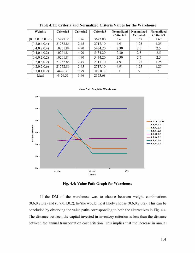
101
Table 4.11: Criteria and Normalized Criteria Values for the Warehouse Weights Criteria1 Criteria2 Criteria3 Normalized
Criteria1 Normalized
Criteria2 Normalized
Criteria3 (0.33,0.33,0.33) 15977.35 3.26 3622.80 3.61 1.67 1.67
(0.2,0.4,0.4) 21752.86 2.45 2717.10 4.91 1.25 1.25 (0.4,0.2,0.4) 10201.84 4.90 5434.20 2.30 2.5 2.5 (0.4,0.4,0.2) 10201.84 4.90 5434.20 2.30 2.5 2.5 (0.6,0.2,0.2) 10201.84 4.90 5434.20 2.30 2.5 2.5 (0.2,0.6,0.2) 21752.86 2.45 2717.10 4.91 1.25 1.25 (0.2,0.2,0.6) 21752.86 2.45 2717.10 4.91 1.25 1.25 (0.7,0.1,0.2) 4426.33 9.79 10868.39 1 5 5
Ideal 4426.33 1.96 2173.68
Fig. 4.4: Value Path Graph for Warehouse
If the DM of the warehouse was to choose between weight combinations
(0.6,0.2,0.2) and (0.7,0.1,0.2), he/she would most likely choose (0.6,0.2,0.2). This can be
concluded by observing the value paths corresponding to both the alternatives in Fig. 4.4.
The distance between the capital invested in inventory criterion is less than the distance
between the annual transportation cost criterion. This implies that the increase in annual
102
transportation cost is more than the decrease in capital invested in inventory. Assuming
that the DM chooses weight combination (0.6,0.2,0.2) as the most preferred solution, the
warehouse�s ordering policy is to order 355.42 units when the reorder point reaches 47.67
units. The time between orders is 10.62 weeks.
The weight shipped for the weight combination (0.7,0.1,0.2) is 7108.4 lbs which
is less than 18256 lbs, the weight requirement for using the inverse function. As a result
the annual transportation cost is overestimated. If a power function was used, the annual
transportation cost would be $5150.08. Hence, the DM of the warehouse might have to
consider using LTL shipments instead of TL shipments if they want to choose weight
combination (0.7,0.1,0.2).
4.8 Summary
In this chapter we extended the single objective cost model of the previous
chapter to a multi-criteria framework where marginal cost information is not known.
Transportation costs were considered between the echelons. Under the assumption that
the retailers� shipments were LTL and the warehouse�s shipment was TL a MCMP was
developed. The Pλ method in conjunction with a graphical tool called the Value Path
Method was used to assist the DM in choosing the most preferred solution. The impact
of transportation costs on the ordering policy of each location was studied. Relaxing the
previous assumption, another MCMP was developed which not only determines the
ordering policies of the companies but also indicates when to use TL and when to use
LTL. An example problem was used to explain the methodology.
In the next chapter we develop and solve the multi-criteria supply chain inventory
problem with transportation costs by relaxing the assumptions on demands and lead
times. The external demands faced by the retailers are non-identical random variables,
and the lead times follow a general discrete distribution.

103
Chapter 5
STOCHASTIC MULTI-CRITERIA MODEL FOR A SUPPLY CHAIN WITH TRANSPORTATION
COSTS
5.1 Introduction
In this chapter we extend the basic model of Chapter 4 to the case where there is
randomness in the system due to the external demand faced by the retailers and the
replenishment time required to fulfill the orders placed by each company in the supply
chain. We model the supply chain as a multi-criteria problem with four criteria. In
addition to the three criteria of the previous chapter, capital invested in inventory, annual
number of orders and annual transportation costs, a customer service criterion is included.
The objective in this chapter is to develop relatively simple, yet realistic, models and
solution procedures that can be implemented in practice.
5.2 Problem Description
The system under consideration is the same as in Chapters 3 and 4. We are
interested in determining ordering policies for each location in a single warehouse multi-
retailer system. The warehouse is supplied by a manufacturer that is assumed to have
infinite capacity. The retailers face independent but non-identical stochastic demands.
Further, the lead times between the stages are assumed to be discrete random variables.
Transportation costs are considered between the echelons. The inbound transportation
cost at the retailer and the warehouse is modeled using LTL and TL rates, respectively.
The optimization problem for each location is modeled as a multi-criteria problem. A
general model for determining the retailer inventory policy is presented. Depending upon
the distribution of the lead time demand three variants of this model are discussed. Then,
using the output of all the retailers, we formulate and solve the warehouse�s inventory
problem.
5.2.1 Assumptions
• Each location follows a continuous review policy, i.e., an order is placed when the
inventory level reaches the reorder point; however instead of continuous tracking,

104
it is enough if each transaction is recorded when it occurs, and the inventory
levels are adjusted after the transaction has been finalized. This is called a
transactions reporting system. For the system to place an order precisely when
the inventory level reaches the reorder point the system must be monitored
continuously or demand must occur one at a time. In cases where the number of
units ordered when a demand occurs exceeds one or when a transaction reporting
system is used, then the inventory level after the demand has been realized might
have overshot the reorder point. This is called demand overshoot, which leads us
to the next assumption.
• The probability of a large overshoot is very small which means that when it
occurs, it is very small compared to the lead time demand.
• Excess demand at each location is treated as lost sales. While most of the
literature in supply chain inventory models assume that excess demand is
backordered, this may not be true particularly at the retailer for functional
products since a customer who enters a retail shop is not going to wait for an item
if it is not in the shelf. He/she is going to purchase that item elsewhere. Excess
demand at the warehouse is treated as lost sales since the supply chain is
operating under a decentralized control.
• There is no order splitting at the warehouse, i.e., if the warehouse is not able to
completely meet an order, the entire order is lost. This is a realistic assumption
since the freight rate is a function of the retailer�s order quantity.
• The average time that any location is out of stock is negligible compared to its
reorder interval. Again, this is a realistic assumption due to the high level of
service requirements imposed on each company.
• There is no outstanding order at time of reorder. This implies that the reorder
point is less than the order quantity.
• The mean rate of demand does not vary with time (the demand distributions are
stationary).
• Orders do not crossover, i.e., orders arrive in the same order they are placed.
105
• FOB origin is assumed at each location. This means that the retailers take
ownership of the goods at the warehouse and the warehouse takes ownership of
the goods at the manufacturer and pay for in transit inventory.
5.2.2 Notation
Data
iD - Expected annual demand for retailer i
Diµ - Mean demand for retailer i during a time period t
Diσ - Standard deviation of demand for retailer i during a time period t
WD - Expected annual demand at the warehouse
DWµ - Mean demand at the warehouse during a time period t
DWσ - Standard deviation of demand at the warehouse during a time period t
iL - Lead time for retailer i with distribution { } jii pjLPr == (random variable)
Liµ - Mean lead time for retailer i
Liσ - Standard deviation of lead time for retailer i
WL - Lead time for the warehouse with distribution { } jWW pjLPr == (random variable)
LWµ - Mean lead time for warehouse
LWσ - Standard deviation of lead time for warehouse
iLD - Demand during the lead time for retailer i (random variable)
LDiµ - Mean lead time demand for retailer i
LDiσ - Standard deviation of lead time demand for retailer i
WLD - Demand during the lead time for warehouse (random variable)
LDWµ - Mean lead time demand for warehouse
LDWσ - Standard deviation of lead time demand for warehouse
iC - Cost/unit at retailer i ∀ i=1,2,�, N
WC - Cost/unit at warehouse
ω- Weight of a single unit in lbs
yiF - Proportional freight rate function for retailer i given by ( )yixiixiyi WWFF −α+=
106
Fxi- TL freight rate for each retailer ($/cwt)
Wxi-TL weight
Wyi- Weight shipped to each retailer i (lbs)
αi - Rate at which freight rate increases / 100lbs decrease in shipping weight for retailer i.
yWF - Inverse freight rate function for warehouse given by yW
xWxWyW W
WFF =
FxW- TL freight rate for the warehouse ($/cwt)
WxW -TL weight for the warehouse
WyW- Weight of the order quantity shipped to the warehouse (lbs)
N- Number of retailers
Decision Variables
iQ � Order quantity of retailer i
WQ � Order quantity of warehouse
ir � Reorder point for retailer i
Wr � Reorder point for warehouse
is - Safety stock for retailer i (expected on hand inventory at the time when new order
arrives)
Ws - Safety stock for warehouse
iESC - Expected shortages/order cycle (lost sales) for retailer i
WESC - Expected shortages/order cycle (lost sales) for warehouse
5.3 Retailer�s Model Formulation
When the demand faced by a retailer that is following a continuous review policy
is stochastic, the reorder interval, i.e., time between orders is a random variable but the
order quantity is fixed. There is a possibility that the lead time demand (LTD), which is
now a random variable, may exceed the reorder point and leading to a stockout. To
minimize stockouts, a safety stock is maintained. Safety stock is defined as the expected
on-hand inventory when an order arrives. Safety stock is usually determined based on
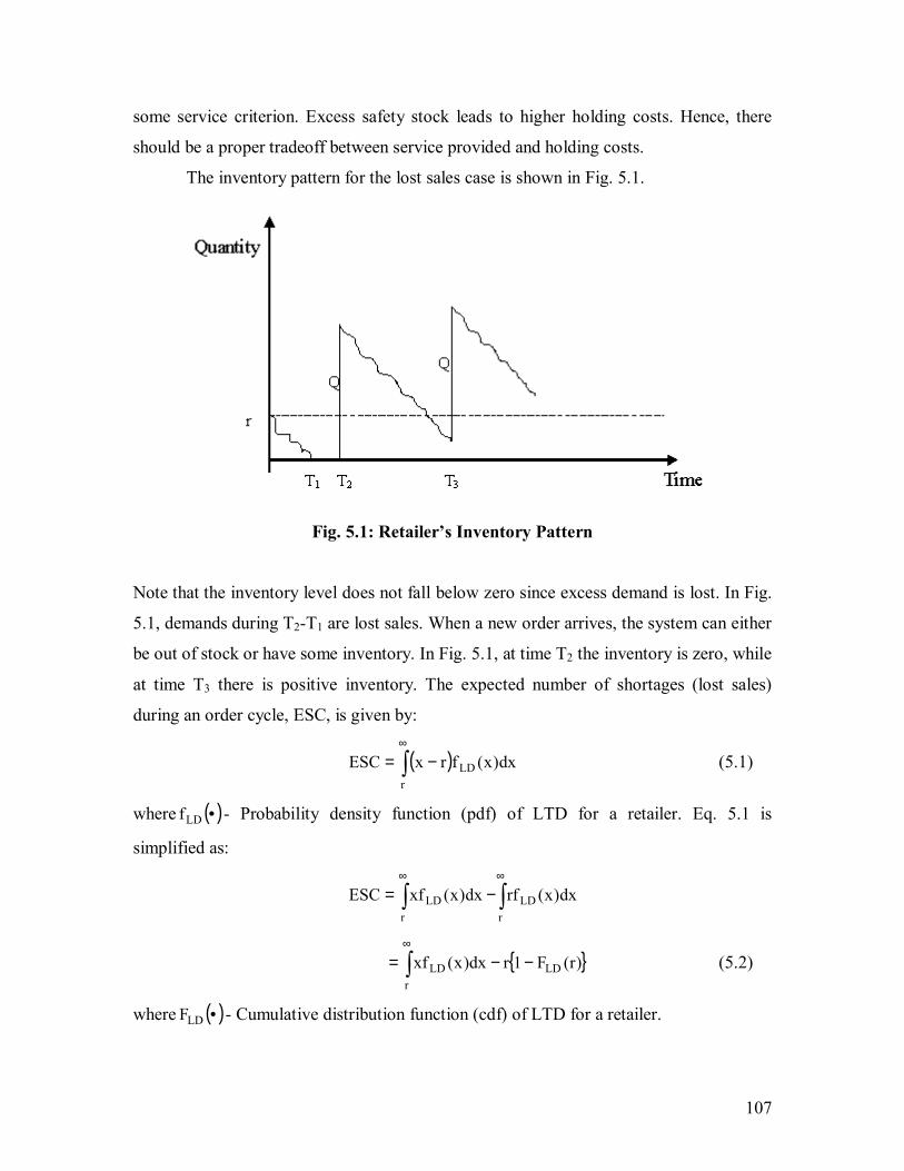
107
some service criterion. Excess safety stock leads to higher holding costs. Hence, there
should be a proper tradeoff between service provided and holding costs.
The inventory pattern for the lost sales case is shown in Fig. 5.1.
Fig. 5.1: Retailer�s Inventory Pattern
Note that the inventory level does not fall below zero since excess demand is lost. In Fig.
5.1, demands during T2-T1 are lost sales. When a new order arrives, the system can either
be out of stock or have some inventory. In Fig. 5.1, at time T2 the inventory is zero, while
at time T3 there is positive inventory. The expected number of shortages (lost sales)
during an order cycle, ESC, is given by:
( )∫∞
−=r
LD dx)x(frxESC (5.1)
where ( )•LDf - Probability density function (pdf) of LTD for a retailer. Eq. 5.1 is
simplified as:
∫∫∞∞
−=r
LDr
LD dx)x(rfdx)x(xfESC
{ })r(F1rdx)x(xf LDr
LD −−= ∫∞
(5.2)
where ( )•LDF - Cumulative distribution function (cdf) of LTD for a retailer.
108
Following Ravindran et al. (1987, Chapter 8, pp. 356-364), the expected on-hand
inventory when a new order arrives is the safety stock, s, and is determined as:
( )∫∞
−=0
LD dx)x(fxrs
Note that the inventory level at the time when new order arrives is:
r � x if x ≤ r
0 if x > r
Hence,
( ) ∫∫∞
+−=r
LD
r
0LD dx)x(f0dx)x(fxrs
The second integral vanishes as any demand in excess of r is lost in the lost sales case.
Hence, the expression for safety stock is:
( )∫ −=r
LD dxxfxrs0
)( (5.3)
Eq. 5.3 is simplified as:
( ) ( )∫∫∞∞
−−−=r
LD0
LD dx)x(fxrdx)x(fxrs
∫∫∫∫∞∞∞∞
+−−=r
LDr
LD0
LD0
LD dx)x(xfdx)x(rfdx)x(xfdx)x(rf
{ } ∫∞
+−−µ−=r
LDLDLD dx)x(xf)r(F1rr (5.4)
Substituting Eq. 5.2 into Eq. 5.4:
ESCrs LD +µ−= (5.5)
Retailer�s Criteria
The following criteria are used in the retailer�s multi-objective problem:
• Capital invested in inventory (including in-transit inventory due to FOB origin)
• Number of orders placed annually
• Annual transportation cost
• Fill rate (service criterion)
109
Criterion 1: Capital Invested in Inventory
As in the previous chapter the capital invested in inventory has two components:
• Capital invested in inventory at Retailer: The expression for average inventory is
based on the approximate lost sales model in Hadley and Whitin (1963, Chapter
4, pp. 162-172) and Ravindran et al. (1987, Chapter 8, pp. 356-364). Since the
expected ending inventory level at the retailer is its safety stock is , the expected
inventory level when an order is received is ii sQ + . The average inventory at the
retailer is ii s
2Q + . Hence, the capital invested in inventory at the retailer is:
+ i
ii s
2Q
C (5.6)
• Capital invested in In-transit inventory: Since the in-transit inventory is affected
only by the mean lead time and not the standard deviation, the expression for the
capital invested in In-transit inventory is the same as in Chapter 4.
365DC iLi
iµ (5.7)
The total capital invested in inventory is given by the sum of Eq. 5.6 and Eq. 5.7:
µ
++365
Ds
2Q
C iLii
ii (5.8)
where iLDiii ESCrs +µ−= .
Criterion 2: Number of Orders Placed Annually
The annual number of orders is still the ratio of the expected annual demand to
the order quantity as the average time spent by the system in a stockout situation is
negligible��due to the high level of service provided by the retailer:
i
i
QD (5.9)
�� If the assumption is relaxed, the number of orders placed is
sDTQ
Dµ+
, where sT (T2 � T1 in Fig. 5.1.)
is the average time spent by the system when there is no stock.

110
Criterion 3: Annual Transportation Costs
Since it is assumed that the retailer�s shipments are most likely going to be LTL,
the proportional function§§ is used to model the transportation cost. The annual
transportation cost is given by:
{ }100D
QW(F iixiixi
ωω−α+ (5.10)
Criterion 4: Fill Rate (FR)
As explained previously, the safety stock is set based on service commitments
promised by each location. A fill rate criterion is used to model the service criterion. Fill
rate is defined as the proportion of demand that is met from available stock.
Mathematically it is defined as:
i
ii Q
ESC1FR −=
We would like to maximize fill rate or minimize the fraction of demand lost.
Hence, the fourth criterion is:
i
ii Q
ESCFR1 =− (5.11)
5.3.1 Retailer�s Multi-Criteria Problem
Each retailer�s MCMP consists of minimizing capital invested in inventory (Eq.
5.8), annual number of order (Eq. 5.9), annual transportation cost (Eq. 5.10), and fraction
of demand not met (Eq. 5.11) simultaneously and is given as:
§§ In the example problem of Chapter 4, we concluded that a power function best estimates LTL rates, but using the proportional function enables us to develop closed form expressions. We revert to using the power function for the example problem.

111
Retailer�s Multi-criteria Problem (Ri)
Min
µ
++µ−+=365
DESCr
2Q
CZ iLiiLDii
ii
1i {Using Eq. 5.5}
Mini
i2i Q
DZ =
Min { }100D
QW(FZ iixiixi
3i
ωω−α+=
Mini
i4i Q
ESCZ =
:.t.s 0Qi ≥
0ri ≥
5.3.2 Solution Procedure to Solve Problem (Ri)
Using the same Pλ method discussed in Chapter 4, the MCMP is converted into a
single objective problem:
Problem )( λiR
{ }
i
i4i
iixiixi
3i
i
i2i
iLiiLDii
ii
1ii
QESC
100D
QW(FQD
365D
ESCr2
QCZMin
λ+
ωω−α+λ+λ+
µ
++µ−+λ=λ
:.t.s 13
1k
ki =λ∑
=
0ki >λ k,i∀
0Qi ≥ i∀
0ri ≥
kiλ - Convex combination parameter or weight assigned for criterion k for retailer i.
For the weighted objective method to perform well, the individual criteria must be
scaled. We utilize the following normalization scheme:
*ki*
ki
*ki
kikn
iZZ
ZZZ−
−=
112
where:
kniZ - Normalized value of criterion k for retailer i
*k
iZ - Lowest value or ideal solution of criterion k for retailer i
*kiZ - Largest value or anti-ideal solution of criterion k for retailer i
This normalization scheme guarantees kniZ to be between 0 and 1.
Then Problem ( λiR ) can be rewritten as:
{ }
−
−λ+
−
−ωω−α+λ
+
−
−λ+
−
−µ++µ−+λ=λ
*4i*
4i
*4i
i
i
4i*3
i*3i
*3i
iixiixi
3i
*2i*
2i
*2i
i
i
2i*1
i*1i
*1i
iLiiLDii
ii
1ii
ZZ
ZQ
ESC
ZZ
Z100DQW(F
ZZ
ZQD
ZZ
Z365
DESCr2
QCZMin
{ }
−λ+
−
ωω−α+λ
+
−λ+
−
µ++µ−+λ=λ
*4i
i
in4i
*3i
iixiixi
n3i
*2i
i
in2i
*1i
iiL
iiLTDi
ii
n1ii
ZQ
ESCZ
100D
QW(F
ZQDZ
365DESCr
2QCZMin
where *ki*
ki
kikn
iZZ −
λ=λ , the normalized/scaled weight for criterion k for retailer i.
Before we solve the Pλ problem, we have to make sure the objective functions are
convex. We know that the first three criteria are convex. Also, the annual number of
orders criterion is strictly convex. From Hadley and Whitin (Chapter 4, pp. 220-221),
QESC is also convex. Since the weighted sum of convex functions is a convex function,
λiZ is convex.
Computing the partial derivative of λiZ with respect to Qi and setting it to zero:
0Q
ESC100
DQD
2C
QZ
2i
in4i
2iin3
i2i
in2i
in1i
i
i =λ−
ωα−λ+λ−λ=∂∂ λ
113
Let ω=ω 1002
{ } ωαλ−λ=λ+λ iin3
iin1
iin4
iin2
i2i
D2
CESCD
Q1
{ }ωαλ−λ
λ+λ=⇒
iin3
iin1i
in4
iin2
ii D2C
ESCD2Q (5.12)
Computing the partial derivative of λiZ with respect to ri and setting it to zero:
0r
ESCQ1
rs
Cr
Z
i
i
i
n4i
i
ii
n1i
i
i =∂
∂λ+
∂∂
λ=∂
∂ λ
Using Eq. 5.1 and Eq. 5.5 for ESCi and si, respectively, and using the Leibnitz rule***:
( ){ } ( ){ } 0)r(F)r(fr1)r(frQ
)r(F)r(fr1)r(fr1C iLDiiLDiiLDiii
n4i
iLDiiLDiiLDiiin1i =−−−−
λ+−−−−λ
{ } 0)r(F1Q
CC LDii
n4i
in1ii
n1i =−
λ+λ−λ
{ }
λ+λ
λ=−
i
n4i
in1i
in1i
iLDi
QC
C)r(F1 (5.13)
In Eq. 5.13, )(rFLD is called the cycle service level (CSL) and is defined as the
probability of not having a stockout in a cycle. Mathematically CSL is ∫r
0LD dx)x(f . Since
n1iλ and n4
iλ are positive and the RHS of Eq. 5.13 is between 0 and 1, there will always be
a solution. The LHS of Eq. 5.13 is nothing but the probability that lead time demand
exceeds the reorder point. We can make the following observations from Eq. 5.13:
0r1
QC
Ci
i
n4i
in1i
in1i →⇒→
λ+λ
λ (5.14)
*** Leibnitz rule: ( ) ( )r),r(fdrdr),r(f
drddx
r)r,x(fdx)r,x(f
drd )r(
)r(
)r(
)r(
χχ−ψψ+∂
∂= ∫∫ψ
χ
ψ
χ
(Nahmias, 2001)
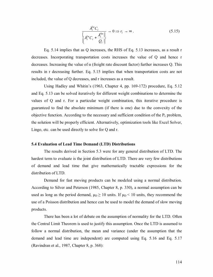
114
∞→⇒→
+i
i
ni
in
i
in
i r
QC
C0
41
1
λλ
λ. (5.15)
Eq. 5.14 implies that as Q increases, the RHS of Eq. 5.13 increases, as a result r
decreases. Incorporating transportation costs increases the value of Q and hence r
decreases. Increasing the value of α (freight rate discount factor) further increases Q. This
results in r decreasing further. Eq. 5.15 implies that when transportation costs are not
included, the value of Q decreases, and r increases as a result.
Using Hadley and Whitin�s (1963, Chapter 4, pp. 169-172) procedure, Eq. 5.12
and Eq. 5.13 can be solved iteratively for different weight combinations to determine the
values of Q and r. For a particular weight combination, this iterative procedure is
guaranteed to find the absolute minimum (if there is one) due to the convexity of the
objective function. According to the necessary and sufficient condition of the Pλ problem,
the solution will be properly efficient. Alternatively, optimization tools like Excel Solver,
Lingo, etc. can be used directly to solve for Q and r.
5.4 Evaluation of Lead Time Demand (LTD) Distributions
The results derived in Section 5.3 were for any general distribution of LTD. The
hardest term to evaluate is the joint distribution of LTD. There are very few distributions
of demand and lead time that give mathematically tractable expressions for the
distribution of LTD.
Demand for fast moving products can be modeled using a normal distribution.
According to Silver and Peterson (1985, Chapter 8, p. 330), a normal assumption can be
used as long as the period demand, µD ≥ 10 units. If µD < 10 units, they recommend the
use of a Poisson distribution and hence can be used to model the demand of slow moving
products.
There has been a lot of debate on the assumption of normality for the LTD. Often
the Central Limit Theorem is used to justify this assumption. Once the LTD is assumed to
follow a normal distribution, the mean and variance (under the assumption that the
demand and lead time are independent) are computed using Eq. 5.16 and Eq. 5.17
(Ravindran et al., 1987, Chapter 8, p. 368):

115
LDLD µµ=µ (5.16)
2L
2D
2DL
2LD σµ+σµ=σ (5.17)
Eppen and Martin (1988) and Tyworth (1991) state that specifying the LTD
incorrectly as a normal distribution can lead to inaccurate estimates of safety stock. It can
also be argued, however, that even though the deviations in safety stock costs may be
large, it may not be significant when compared to cycle stock costs, ordering costs, etc.
We consider three cases:
• Case 1 is for a slow moving product where the demand follows a Poisson
distribution and the lead time is a general discrete distribution. This implies that
when a demand occurs, only one unit is ordered by the customer.
• Case 2 is again for slow moving products where the demand follows a geometric
Poisson process (special case of Compound Poisson process) and the lead time is
a general discrete distribution. In this case when a demand occurs, a customer can
order more than one unit.
• Case 3 is for a fast moving product and is the normal approximation for Case 1
and Case 2. Here, the demand follows a normal distribution, while the lead time is
a general discrete distribution.
5.4.1 Case 1: Demand-Poisson Distribution, Lead Time-General Discrete
Distribution
The retailer demand is assumed to follow a Poisson distribution and is denoted
as ( )DiP µ . The mean and variance of a Poisson distribution are equal to Diµ . The lead time
follows a discrete distribution given by { } jii pjLPr == . Given that Li = j, the conditional
distribution of LTD still follows a Poisson distribution given by jiLD ~ ( )DijP µ . Thus, the
conditional probability mass function (pmf) of the LTD (omitting the subscript i) is:
( )!x
je)x(px
jjLD
µ= µ− (5.18)
Eq. 5.18 is used to determine the expected shortages/reorder cycle (ESC) and
hence, the safety stock. ESC is determined in two steps. First, we determine the expected
shortages by conditioning on the lead time:
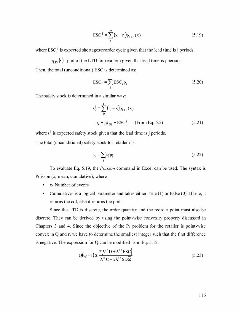
116
( )∑∞
−=ir
jLDii
ji )x(prxESC (5.19)
where jiESC is expected shortages/reorder cycle given that the lead time is j periods.
( )•jLDip - pmf of the LTD for retailer i given that lead time is j periods.
Then, the total (unconditional) ESC is determined as:
ji
j
jii pESCESC ∑= (5.20)
The safety stock is determined in a similar way:
( )∑ −=ir
0
jLDii
ji )x(pxrs
jiDii ESCjr +µ−= (From Eq. 5.5) (5.21)
where jis is expected safety stock given that the lead time is j periods.
The total (unconditional) safety stock for retailer i is:
ji
j
jii pss ∑= (5.22)
To evaluate Eq. 5.19, the Poisson command in Excel can be used. The syntax is
Poisson (x, mean, cumulative), where
• x- Number of events
• Cumulative- is a logical parameter and takes either True (1) or False (0). If true, it
returns the cdf, else it returns the pmf.
Since the LTD is discrete, the order quantity and the reorder point must also be
discrete. They can be derived by using the point-wise convexity property discussed in
Chapters 3 and 4. Since the objective of the Pλ problem for the retailer is point-wise
convex in Q and r, we have to determine the smallest integer such that the first difference
is negative. The expression for Q can be modified from Eq. 5.12.
( ) { }ωαλ−λ
λ+λ≥+
D2C
ESCD21QQ n3n1
n4n2
(5.23)

117
Q can be determined by finding the smallest integer that satisfies the condition given by
Eq. 5.23. However, the expression for r cannot be deduced from Eq. 5.13. To determine r,
we start of by computing the first difference of λZ with respect to r:
0)r,Q(Z)1r,Q(Z)1r,Q(Z ≥−+=+∆ λλλ
( ) ( ) 0ESCQ
ESCrCESCQ
ESC1rC r
n4
rLDn1
1r
n4
1rLDn1 ≥λ−+µ−λ−λ++µ−+λ ++
{ } 0ESCESCQ
CC r1r
n4n1n1 ≥−
λ+λ+λ + (5.24)
r can be determined by finding the smallest integer that satisfies Eq. 5.24. Since Eq. 5.24
is more cumbersome when compared to Eq. 5.13 for determining r, a continuous
approximation for the discrete case can be used. Hadley and Whitin (1963, Chapter 4, p.
190) recommend that Q can be approximated by using Eq. 5.12 when Q ≥ 10, and r can
be approximated using Eq. 5.13 when µLD ≥ 25.
5.4.2 Case 2: Demand-Compound Poisson Distribution, Lead Time-General Discrete
Distribution
As mentioned before a Poisson distribution can be used to model the demand of
slow moving products. When demand follows a Poisson distribution, demand occurs one
at a time, and the variance to mean ratio is one. However, a customer going to a retailer
may buy several quantities of the same product. Further, Nahmias and Smith (1994)
assert that the variance to mean ratio is often greater than 1. A compound Poisson
distribution can be used to model these two conditions.
A compound Poisson process is a stochastic process wherein demand occurs
according to a Poisson distribution and the number of units demanded per demand
occurrence is a positive discrete random variable. The total number of units demanded in
a time period t is given by:
( ) ∑=
=)t(N
1iiYtX
where,
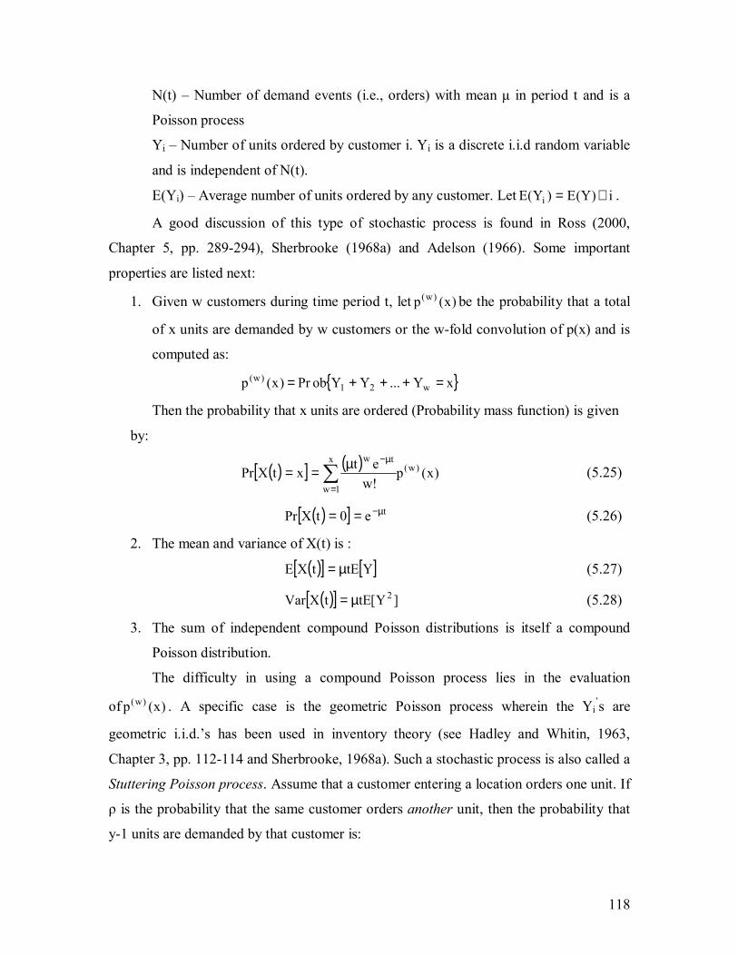
118
N(t) � Number of demand events (i.e., orders) with mean µ in period t and is a
Poisson process
Yi � Number of units ordered by customer i. Yi is a discrete i.i.d random variable
and is independent of N(t).
E(Yi) � Average number of units ordered by any customer. Let i)Y(E)Y(E i ∀= .
A good discussion of this type of stochastic process is found in Ross (2000,
Chapter 5, pp. 289-294), Sherbrooke (1968a) and Adelson (1966). Some important
properties are listed next:
1. Given w customers during time period t, let )x(p )w( be the probability that a total
of x units are demanded by w customers or the w-fold convolution of p(x) and is
computed as:
{ }xY...YYobPr)x(p w21)w( =+++=
Then the probability that x units are ordered (Probability mass function) is given
by:
( )[ ] ( ) )x(p!wetxtXPr )w(
x
1w
tw
∑=
µ−µ== (5.25)
( )[ ] te0tXPr µ−== (5.26)
2. The mean and variance of X(t) is :
( )[ ] [ ]YtEtXE µ= (5.27)
( )[ ] ]Y[tEtXVar 2µ= (5.28)
3. The sum of independent compound Poisson distributions is itself a compound
Poisson distribution.
The difficulty in using a compound Poisson process lies in the evaluation
of )x(p )w( . A specific case is the geometric Poisson process wherein the Yi�s are
geometric i.i.d.�s has been used in inventory theory (see Hadley and Whitin, 1963,
Chapter 3, pp. 112-114 and Sherbrooke, 1968a). Such a stochastic process is also called a
Stuttering Poisson process. Assume that a customer entering a location orders one unit. If
ρ is the probability that the same customer orders another unit, then the probability that
y-1 units are demanded by that customer is:
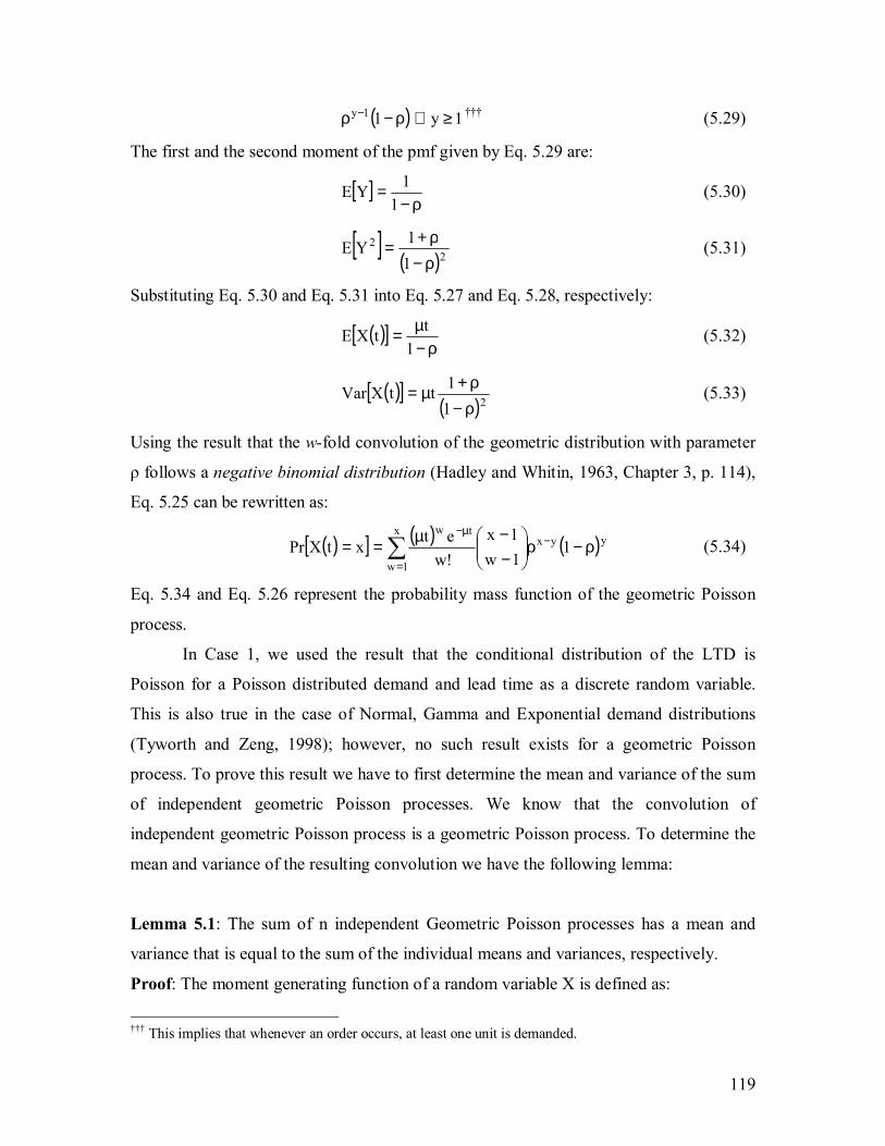
119
( ) 1y11y ≥∀ρ−ρ − ��� (5.29)
The first and the second moment of the pmf given by Eq. 5.29 are:
[ ]ρ−
=1
1YE (5.30)
[ ]( )2
2
11YE
ρ−ρ+= (5.31)
Substituting Eq. 5.30 and Eq. 5.31 into Eq. 5.27 and Eq. 5.28, respectively:
( )[ ]ρ−
µ=1
ttXE (5.32)
( )[ ]( )211ttXVar
ρ−ρ+µ= (5.33)
Using the result that the w-fold convolution of the geometric distribution with parameter
ρ follows a negative binomial distribution (Hadley and Whitin, 1963, Chapter 3, p. 114),
Eq. 5.25 can be rewritten as:
( )[ ] ( ) ( )yyxx
1w
tw1
1w1x
!wetxtXPr ρ−ρ
−−µ== −
=
µ−
∑ (5.34)
Eq. 5.34 and Eq. 5.26 represent the probability mass function of the geometric Poisson
process.
In Case 1, we used the result that the conditional distribution of the LTD is
Poisson for a Poisson distributed demand and lead time as a discrete random variable.
This is also true in the case of Normal, Gamma and Exponential demand distributions
(Tyworth and Zeng, 1998); however, no such result exists for a geometric Poisson
process. To prove this result we have to first determine the mean and variance of the sum
of independent geometric Poisson processes. We know that the convolution of
independent geometric Poisson process is a geometric Poisson process. To determine the
mean and variance of the resulting convolution we have the following lemma:
Lemma 5.1: The sum of n independent Geometric Poisson processes has a mean and
variance that is equal to the sum of the individual means and variances, respectively.
Proof: The moment generating function of a random variable X is defined as:
��� This implies that whenever an order occurs, at least one unit is demanded.

120
( ) ( )∑==φs
sxsx spe]e[Es
The first and second moments of X can then be determined by computing the first and
second differentials:
)0(]X[E 'φ=
)0(]X[E "2 φ=
The variance is computed as:
{ } 22 ]X[E]X[E]X[Var −=
The moment generating function of a compound Poisson process
( ) ( )( ){ }s1texps Yφ−µ−=φ (5.35)
( )sYφ is the moment generating function of number of units demanded defined by
random variable Y. Since Y is geometrically distributed, its moment generating function
is given by:
( ) ( )s
s
Y e1e1s
ρ−ρ−=φ (5.36)
Substituting Eq. 5.36 into Eq. 5.35, we get the moment generating function of the
geometric compound Poisson process as:
( )
ρ−−µ−=φ s
s
e1e1texps (5.37)
Let X1(t) and X2(t) be two independent geometric Poisson processes and X(t) be
the convolution of X1(t) and X2(t), i.e.,
( ) ( ) ( )tXtXtX 21 +=
The moment generating function of X(t) is the product of the moment generating
functions of X1(t) and X2(t):
( ) ( ) ( )sss 21 φφ=φ
ρ−−µ−
ρ−−µ−= s
2
s
2s1
s
1 e1e1texp
e1e1texp
ρ−−µ−
ρ−−µ−= s
2
s
2s1
s
1 e1e1t
e1e1texp
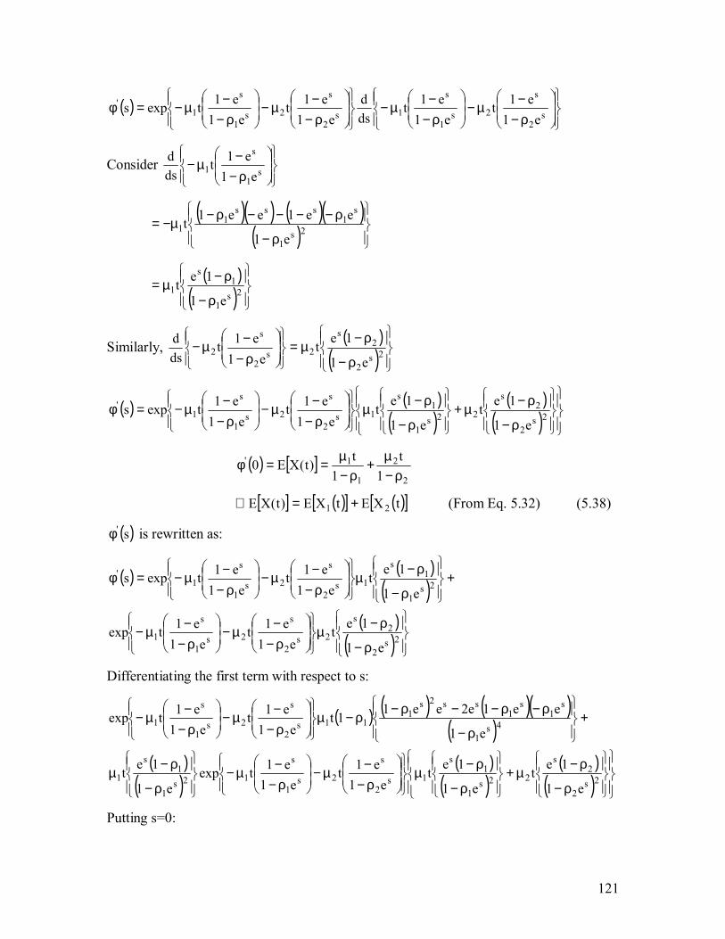
121
( )
ρ−−µ−
ρ−−µ−
ρ−−µ−
ρ−−µ−=φ s
2
s
2s1
s
1s2
s
2s1
s
1'
e1e1t
e1e1t
dsd
e1e1t
e1e1texps
Consider
ρ−−µ− s
1
s
1 e1e1t
dsd
( )( ) ( )( )( )
ρ−
ρ−−−−ρ−µ−= 2s1
s1
sss1
1e1
ee1ee1t
( )( )
ρ−
ρ−µ= 2s1
1s
1e1
1et
Similarly, ( )( )
ρ−
ρ−µ=
ρ−−µ− 2s
2
2s
2s2
s
2e1
1ete1
e1tdsd
( ) ( )( )
( )( )
ρ−
ρ−µ+
ρ−
ρ−µ
ρ−−µ−
ρ−−µ−=φ 2s
2
2s
22s1
1s
1s2
s
2s1
s
1'
e1
1ete1
1ete1
e1te1
e1texps
( ) [ ]2
2
1
1'
1t
1t)t(XE0
ρ−µ+
ρ−µ==φ
[ ] ( )[ ] ( )[ ]tXEtXE)t(XE 21 +=∴ (From Eq. 5.32) (5.38)
( )s'φ is rewritten as:
( ) ( )( )
( )( )
ρ−
ρ−µ
ρ−−µ−
ρ−−µ−
+
ρ−
ρ−µ
ρ−−µ−
ρ−−µ−=φ
2s2
2s
2s2
s
2s1
s
1
2s1
1s
1s2
s
2s1
s
1'
e1
1ete1
e1te1
e1texp
e1
1ete1
e1te1
e1texps
Differentiating the first term with respect to s:
( ) ( ) ( )( )( )
( )( )
( )( )
( )( )
ρ−
ρ−µ+
ρ−
ρ−µ
ρ−−µ−
ρ−−µ−
ρ−
ρ−µ
+
ρ−
ρ−ρ−−ρ−ρ−µ
ρ−−µ−
ρ−−µ−
2s2
2s
22s1
1s
1s2
s
2s1
s
12s1
1s
1
4s1
s1
s1
ss2s1
11s2
s
2s1
s
1
e1
1ete1
1ete1
e1te1
e1texpe1
1et
e1
ee1e2ee11te1
e1te1
e1texp
Putting s=0:

122
( ) ( ) ( )( )( )
ρ−µ+
ρ−µ
ρ−µ+
ρ−ρ−ρ−−ρ−ρ−µ
2
2
1
1
1
14
1
112
111 1
t1
t1
t1
1211t
( )( ) ( )( )21
212
1
12
1
11 11
tt1
t11t
ρ−ρ−µµ+
ρ−
µ+ρ−ρ+µ=
( )( ) ( )( )21
21112
1
1
11ttt1
1t
ρ−ρ−µµ+µ+ρ+
ρ−µ=
Similarly, differentiating the second term and setting s=0 leads to:
( )( ) ( )( )21
21222
2
2
11ttt1
1t
ρ−ρ−µµ+µ+ρ+
ρ−µ
[ ]( )
( ) ( )( ) ( )( ) ( )( )21
21222
2
2
21
21112
1
12
11ttt1
1t
11ttt1
1t)t(XE
ρ−ρ−µµ+µ+ρ+
ρ−µ+
ρ−ρ−µµ+µ+ρ+
ρ−µ=∴
(5.39)
Eq. 5.39 gives the second moment of X(t). The variance of X(t) is computed as:
( ) [ ]( )22 )t(XE])t(X[E]t[XVar −=
( )( )
( )( )
2
2
2222
2
22
1
1112
1
1
1tt1
1t
1tt1
1t
ρ−
µ−µ+ρ+ρ−
µ+
ρ−
µ−µ+ρ+ρ−
µ=
[ ]( ) ( )2
2
222
1
11
11t
11t)t(X(Var
ρ−ρ+µ+
ρ−ρ+µ=
[ ] ( )[ ] ( )[ ]tXVartXVar)t(XVar 21 +=∴ (From Eq. 5.33) (5.40)
■
Eq. 5.38 and Eq. 5.40 can be extended to any number of geometric Poisson
processes. Thus, the sum of n independent geometric Poisson processes is a geometric
Poisson process whose mean equals the sum of the individual means and variance equals
the sum of the individual variances.
Corollary 5.1: If the individual geometric Poisson processes are identical then the
resulting geometric compound process is the n-fold convolution, and hence Eq. 5.38 and
Eq. 5.40 simplify to:
[ ] ( )[ ]tXnE)t(XE 1= (5.41)
[ ] ( )[ ]tXnVar)t(XVar 1= (5.42)
123
Theorem 5.1: If the demand process follows a geometric Poisson process with
parameters ( )( )
ρ−ρ+µ
ρ−µ
211,
1 and the lead time follows a discrete distribution given
by { } jpjLPr == , then the conditional distribution of the lead time demand follows a
geometric Poisson distribution with mean and variance ( )( )
ρ−ρ+µ
ρ−µ
211j,
1j
.
Proof: If the lead time follows a discrete distribution given by { } jpjLPr == and demands
in different periods are independent from one another, the probability mass function of
lead time demand given that lead time is j time units from Feller (1957, Vol.1, Chapter
12, p. 268) is:
)x(p)x(p )j(LD
jLD =
( )•)j(LDp is the probability mass function of the j-fold convolution of demand during one
unit of lead time. Since the demand during unit of lead time follows a geometric Poisson
distribution, the j-fold convolution from corollary 5.1 has mean and variance given by
Eq. 5.41 and Eq. 5.42. Thus, we have proved that if the demand process follows a
geometric Poisson distribution and the lead time follows a discrete distribution, the
conditional distribution of LTD follows a geometric Poisson distribution with mean and
variance ( )( )
ρ−ρ+µ
ρ−µ
211j,
1j
.
■
Thus, the conditional pmf of LTD is:
( ) ( ) ( )yyxx
1w
jwjLD 1
1w1x
!wejxp ρ−ρ
−−µ= −
=
µ−
∑ (5.43)
Unfortunately, Excel does not have a built-in function to evaluate Eq. 5.43.
However, tables like the one in Sherbrooke (1968a) can be used to evaluate Eq. 5.43 and
hence, Eq. 5.19, Eq. 5.20, Eq. 5.21 and Eq. 5.22.

124
5.4.3 Case 3: Demand-Normal Distribution, Lead Time-General Discrete
Distribution
This case can be used when demand is normally distributed as ( )2DiDi ,N σµ or as
approximations to the previous two cases. For large values of Diµ , the Poisson and
compound Poisson distributions can be accurately approximated as a normal distribution.
The lead time follows a discrete distribution given by { } jii pjLPr == . Then the conditional
distribution of LTD still follows a normal distribution given by jiLD ~ ( )2
DiDi j,jN σµ
(Feller, 1957, Vol.1, Chapter 12, p. 268). The conditional pdf is: 2
D
D
jjx
21
D
jLD e
j21)x(f
σµ−
−
σΠ= (5.44)
The expression of the conditional ESC from Eq. 5.2 is { })r(F1rdx)x(xf jLD
r
jLD −−∫
∞
, where
( )•jLDF is the cdf of the lead time demand of a retailer given that lead time is j periods.
Substituting Eq. 5.44 into ∫∞
r
jLD dx)x(xf :
∫∞
=r
jLD dx)x(xf dxxe
j21
r
jjx
21
D
2
D
D
∫∞
σµ−
−
σΠ
Put DD
D jdzdxjjxz σ=⇒σµ−=
∫∞
=r
jLD dx)x(xf dze)jjz(
j21
D
D
2
jjr
2z
DDD∫∞
σµ−
−µ+σ
σΠ
µ+σΠ
=−∞
σµ−
∞
σµ−
−
∫∫ dzejdzejz21 2
z
jjr
D
jjr
2z
D
2
D
D
D
D
2
Consider the first part of the integral:
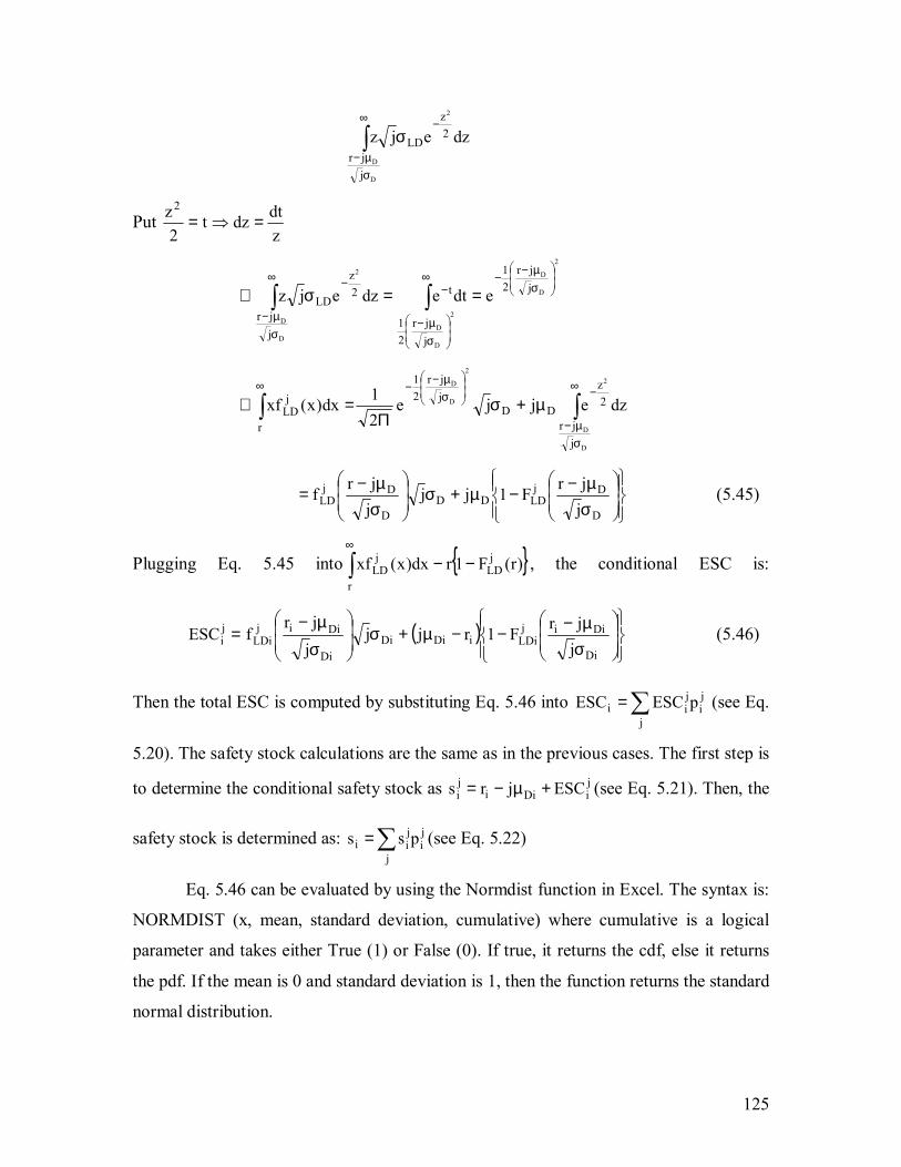
125
∫∞
σµ−
−σ
D
D
2
jjr
2z
LD dzejz
Put zdtdzt
2z2
=⇒=
2
D
D
2
D
DD
D
2
jjr
21
jjr
21
t
jjr
2z
LD edtedzejz
σµ−
−∞
σµ−
−∞
σµ−
−==σ∴ ∫∫
∫∫∞
σµ−
−
σµ−
−∞
µ+σΠ
=∴
D
D
22
D
D
jjr
2z
DDjjr
21
r
jLD dzejje
21dx)x(xf
σµ−−µ+σ
σµ−=
D
DjLDDD
D
DjLD j
jrF1jjjjrf (5.45)
Plugging Eq. 5.45 into { })r(F1rdx)x(xf jLD
r
jLD −−∫
∞
, the conditional ESC is:
=jiESC ( )
σµ−−−µ+σ
σ
µ−
Di
DiijLDiiDiDi
Di
DiijLDi j
jrF1rjjjjr
f (5.46)
Then the total ESC is computed by substituting Eq. 5.46 into ji
j
jii pESCESC ∑= (see Eq.
5.20). The safety stock calculations are the same as in the previous cases. The first step is
to determine the conditional safety stock as jiDii
ji ESCjrs +µ−= (see Eq. 5.21). Then, the
safety stock is determined as: ji
j
jii pss ∑= (see Eq. 5.22)
Eq. 5.46 can be evaluated by using the Normdist function in Excel. The syntax is:
NORMDIST (x, mean, standard deviation, cumulative) where cumulative is a logical
parameter and takes either True (1) or False (0). If true, it returns the cdf, else it returns
the pdf. If the mean is 0 and standard deviation is 1, then the function returns the standard
normal distribution.
126
Note: The model in the previous sections assumed that the lead time was equal to the
transit time. Researchers, e.g., Tyworth and Zeng (1998) and Ganeshan (1999), have
modeled the lead time as the sum of the transit time and a fixed ordering time. The fixed
ordering time can be incorporated as follows. Let P be the fixed order processing time.
Then, the mean of the conditional distribution of LTD is shifted to the right by P, while
the variance remains the same. For example, for Case 3, the distribution of LTD given the
transit time is j periods is jLD ~ ( )2DD j,)Pj(N σµ+ . The rest of the procedure is the same
as in Section 5.4.3.
5.5 Warehouse�s Problem
As in Chapter 4, the warehouse uses the information of the individual retailers to
formulate and hence, determine its ordering policy. The warehouse, like the retailers,
follows a continuous review policy. Excess demand at the warehouse is treated as lost
sales. This assumption was validated by a Fortune 500 company. According to the
company, it does not backorder since none of its customers are willing to wait. The
warehouse is assumed to fill the retailers� orders FIFO (First in First Out). If the
warehouse does not have enough to meet the demand of a particular retailer, the entire
order is lost. It is assumed that the concerned retailer will purchase the order from another
supplier. The lead time of the warehouse is a discrete random variable. The warehouse
has the same criteria as the retailers.
Before we formulate the warehouse�s problem, it is necessary to discuss the
demand process at the warehouse and hence, the LTD distribution. The demand process
at the warehouse is very complicated as it depends on the inventory level of the
individual retailers. Hence, the demand faced by the warehouse is non-stationary.
Deuermeyer and Schwarz (1981), under the assumption of external identical
Poisson demands and complete backorders, characterize the demand process at the
warehouse as an approximate renewal process since the demand process is non-
stationary. After running several simulations, they concluded that the non-stationarity is
not significant. Also, they claim that this approximation is accurate if the warehouse
serves a large number of retailers (N). For N≥20, the above approximation can be safely
used (Ganeshan, 1999).

127
Andersson and Melchiors (2001) explain that even for the one-for-one
replenishment (unit order quantity) policy at the retailers, the demand at the warehouse is
not Poisson under the lost sales assumption. They also approximate the demand process
at the warehouse as a stationary Poisson process.
Since a retailer follows a continuous review policy and the external demands is
Poisson random variables, the time between orders, Ti, is i.i.d. and follows an Erlang-Qi
distribution (Hadely and Whitin, 1963, Chapter 3, p. 112 and Ross, 2000, Chapter 5, pp.
262-263) whose mean and variance is given by:
iD
iTi
Qµ
=µ (5.47)
2Di
i2Ti
Qµ
=σ (5.48)
where Tiµ is mean time between orders for retailer i, and 2Tiσ is variance of time between
orders for retailer i.
Let Ni(t) be the number of orders placed by retailer �i� during period t. Then, Ni(t)
is a renewal process. Let NW(t) be the total number of orders received by the warehouse
during period t. NW(t) is not a renewal process as the order arrival process of the retailers
is dependent on the inventory level at the retailers. Hence, the time between the retailer
orders received by the warehouse is non-identical. In general, NW(t) is a renewal process
only when each retailer�s order quantity is one. Assuming that the non-stationarity is not
significant, NW(t) can be approximated as a renewal process and is given by:
( ) ( )∑=
=N
1iiW tNtN (5.49)
where N is the number of retailers
Determining the exact distribution of NW(t) is difficult and time consuming.
Approximations have been given by Deuermeyer and Schwarz (1981) and Svoronos and
Zipkin (1987) for the identical retailer case. We approximate this renewal process by
applying the central limit theorem for renewal processes (Ross, 2000, Chapter 7, p. 377).
Using this theorem, the renewal processes Ni(t) can be approximated as a normal
distribution for large values of t:

128
µσ
µ∞→ 3Ti
2Ti
Tiit
Lim t,tN~)t(N (5.50)
Substituting Eq. 5.47 and Eq. 5.48 into Eq. 5.50:
µµ2
i
Di
i
Dii
Qt,
QtN~)t(N (5.51)
Eq. 5.51 is the distribution of the number of orders placed by each retailer. The
distribution of the retailer�s orders (demands) is determined by scaling Eq. 5.51 by a
factor Qi and is given as:
( )DiDi t,tN µµ (5.52)
Then the distribution of the total number of orders received by the warehouse during time
period t (using central limit theorem) from Eq. 5.49 and Eq. 5.51 is:
µµ ∑∑==
N
1i2
i
DiN
1i i
DiW
Qt,
QtN~)t(N (5.53)
Similarly, using Eq. 5.52 the distribution of all the retailers� orders (demands) during
time period t is given by:
µµ ∑∑
==
N
1iDi
N
1iDi t,tN (5.54)
Thus, the distribution of period demand at the warehouse is characterized as a
normal distribution with mean and variance give by ∑=
µ=µN
1iDiDW and ∑
=µ=σ
N
1iDi
2DW .
The distribution of demand during the lead time of the warehouse can be characterized as
in Case 3. If the lead time at the warehouse is a discrete distribution given
by { } jWW pjLPr == , then the conditional distribution of LTD at the warehouse given the
lead time is j time units is distributed as ( )2DWDW
jW j,jN~LTD σµ . Now we can
formulate the warehouse�s MCMP.
Note: The demand distribution at the warehouse is characterized as a normal distribution
based on the assumption that the external demands are Poisson. We believe that the
above method can be used for external demands following a geometric Poisson process

129
provided that the probability of a customer ordering more than one unit is less. Since the
Poisson and geometric Poisson random variables can be approximated as a normal
distribution using the central limit theorem, the case of retailers facing normal demands
can also be used.
Warehouse�s Criteria
Criterion 1: Capital Invested in Inventory
The capital invested in inventory consists of 2 components:
• Capital invested in inventory at warehouse: As in the retailer�s problem, the
expected ending inventory level at the warehouse is its safety stock Ws . Then, the
expected inventory level when an order is received is WW sQ + . The average
inventory at the warehouse is approximated as the average of the beginning and
ending inventory levels, i.e., WW s2
Q+ . Hence, the capital invested in inventory
at the warehouse is:
+ W
WW s
2Q
C (5.55)
• Capital invested in in-transit inventory: The capital invested in in-transit
inventory is:
365D
C WLWW
µ (5.56)
The total capital invested in inventory at the warehouse is given by the sum of Eq. 5.55
and Eq. 5.56:
µ
++365
Ds
2Q
C WLWW
WW (5.57)
Criterion 2: Number of Orders Placed Annually
The annual number of orders at the warehouse under the assumption that the
average time spent by the warehouse in a stockout situation is negligible is:
W
W
QD
(5.58)
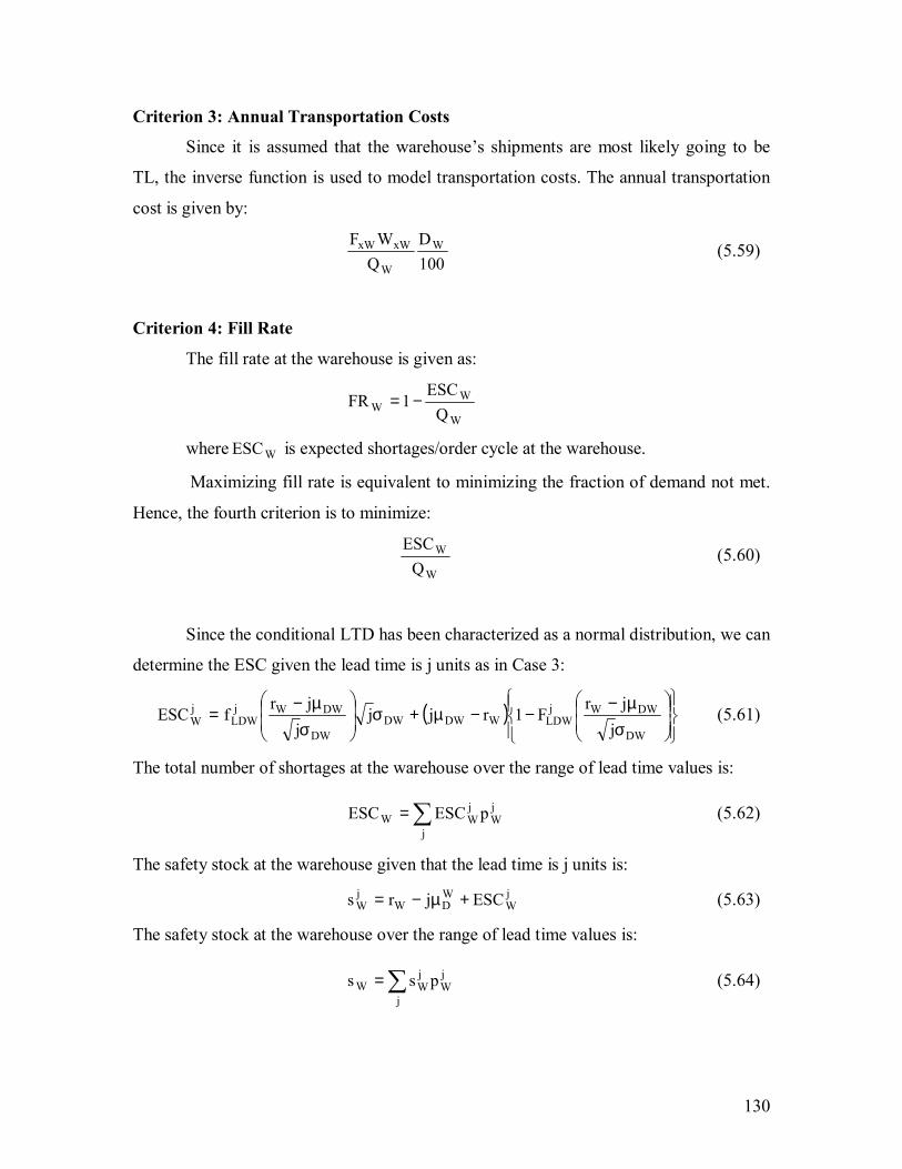
130
Criterion 3: Annual Transportation Costs
Since it is assumed that the warehouse�s shipments are most likely going to be
TL, the inverse function is used to model transportation costs. The annual transportation
cost is given by:
100D
QWF W
W
xWxW (5.59)
Criterion 4: Fill Rate
The fill rate at the warehouse is given as:
W
WW Q
ESC1FR −=
where WESC is expected shortages/order cycle at the warehouse.
Maximizing fill rate is equivalent to minimizing the fraction of demand not met.
Hence, the fourth criterion is to minimize:
W
W
QESC (5.60)
Since the conditional LTD has been characterized as a normal distribution, we can
determine the ESC given the lead time is j units as in Case 3:
=jWESC ( )
σµ−
−−µ+σ
σµ−
DW
DWWjLDWWDWDW
DW
DWWjLDW j
jrF1rjj
jjr
f (5.61)
The total number of shortages at the warehouse over the range of lead time values is:
jW
j
jWW pESCESC ∑= (5.62)
The safety stock at the warehouse given that the lead time is j units is: jW
WDW
jW ESCjrs +µ−= (5.63)
The safety stock at the warehouse over the range of lead time values is:
jW
j
jWW pss ∑= (5.64)
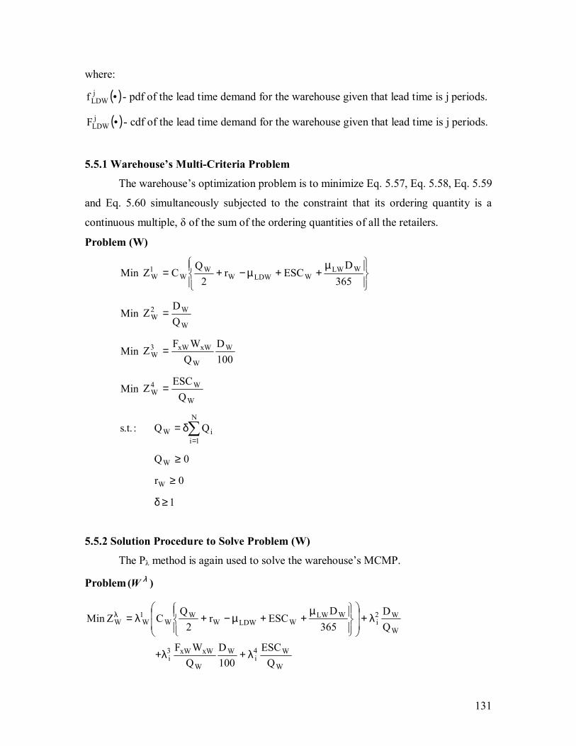
131
where:
( )•jLDWf - pdf of the lead time demand for the warehouse given that lead time is j periods.
( )•jLDWF - cdf of the lead time demand for the warehouse given that lead time is j periods.
5.5.1 Warehouse�s Multi-Criteria Problem
The warehouse�s optimization problem is to minimize Eq. 5.57, Eq. 5.58, Eq. 5.59
and Eq. 5.60 simultaneously subjected to the constraint that its ordering quantity is a
continuous multiple, δ of the sum of the ordering quantities of all the retailers.
Problem (W)
Min
µ
++µ−+=365
DESCr
2Q
CZ WLWWLDWW
WW
1W
MinW
W2W Q
DZ =
Min100D
QWF
Z W
W
xWxW3W =
MinW
W4W Q
ESCZ =
:.t.s ∑=
δ=N
1iiW QQ
0QW ≥
0rW ≥
1≥δ
5.5.2 Solution Procedure to Solve Problem (W)
The Pλ method is again used to solve the warehouse�s MCMP.
Problem )( λW
W
W4i
W
W
xWxW3i
W
W2i
WLWWLDWW
WW
1WW
QESC
100D
QWF
QD
365D
ESCr2
QCZMin
λ+λ+
λ+
µ
++µ−+λ=λ

132
:.t.s ∑=
δ=N
1iiW QQ
13
1k
kW =λ∑
=
0kW >λ k∀
0QW ≥
0rW ≥
1≥δ
where kWλ is the convex combination parameter or weight assigned for criterion k for
warehouse.
As in Problem )R( iλ , the individual criterion must be normalized. Using the same
scheme, Problem ( λW ) can be reformulated as:
−λ+
−λ+
−λ+
−
µ
++µ−+λ=λ
*4W
W
Wn4W
*3W
W
W
xWxWn3W
*2W
W
Wn2W
*1W
WLWWLDWW
WW
n1WW
ZQ
ESCZ
100D
QWF
ZQD
Z365
DESCr
2Q
CZMin
where:
*kW*
kW
kWkn
WZZ −
λ=λ , the normalized/scaled weight for criterion k for warehouse.
*kWZ is the lowest or ideal value of criterion k for warehouse
*kWZ is the largest or anti-ideal value of criterion k for warehouse
Rewriting the objective function of Problem ( λW ) in terms of δ:
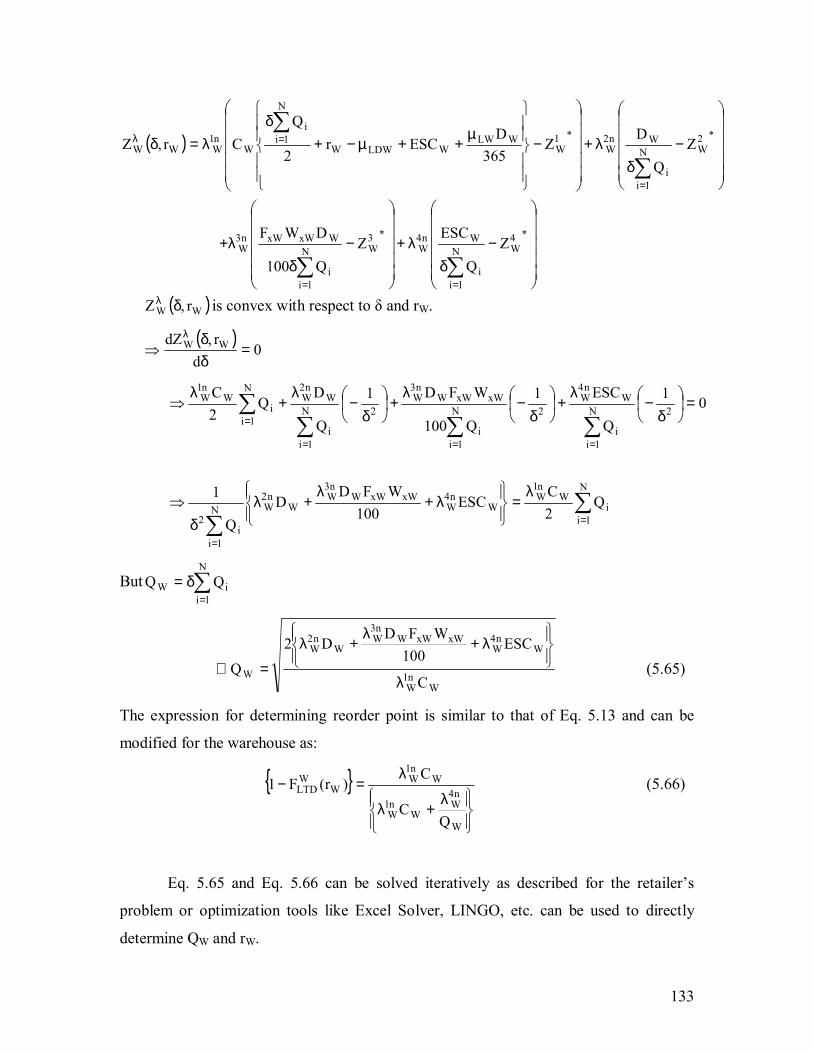
133
( )
−δ
λ+
−δ
λ+
−δ
λ+
−
µ++µ−+
δλ=δ
∑∑
∑
∑
==
=
=λ
*4WN
1ii
Wn4W
*3WN
1ii
WxWxWn3W
*2WN
1ii
Wn2W
*1W
WLWWLDWW
N
1ii
Wn1WWW
ZQ
ESCZ
Q100
DWF
ZQ
DZ
365D
ESCr2
QCr,Z
( )WW r,Z δλ is convex with respect to δ and rW.
( )0
dr,dZ WW =
δδ
⇒λ
01
Q
ESC1
Q100
WFD1
Q
DQ
2C
2N
1ii
Wn4
W2N
1ii
xWxWWn3
W2N
1ii
Wn2
WN
1ii
Wn1W =
δ−
λ+
δ−
λ+
δ−
λ+
λ⇒
∑∑∑∑
===
=
∑∑ =
=
λ=
λ+λ
+λδ
⇒N
1ii
Wn1W
Wn4
WxWxWW
n3W
Wn2
WN
1ii
2Q
2C
ESC100
WFDD
Q
1
But ∑=
δ=N
1iiW QQ
Wn1W
Wn4
WxWxWW
n3W
Wn2
W
W C
ESC100
WFDD2
Qλ
λ+λ
+λ
=∴ (5.65)
The expression for determining reorder point is similar to that of Eq. 5.13 and can be
modified for the warehouse as:
{ }
λ
+λ
λ=−
W
n4W
Wn1W
Wn1W
WWLTD
QC
C)r(F1 (5.66)
Eq. 5.65 and Eq. 5.66 can be solved iteratively as described for the retailer�s
problem or optimization tools like Excel Solver, LINGO, etc. can be used to directly
determine QW and rW.
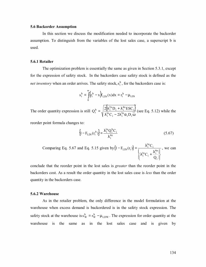
134
5.6 Backorder Assumption
In this section we discuss the modification needed to incorporate the backorder
assumption. To distinguish from the variables of the lost sales case, a superscript b is
used.
5.6.1 Retailer
The optimization problem is essentially the same as given in Section 5.3.1, except
for the expression of safety stock. In the backorders case safety stock is defined as the
net inventory when an order arrives. The safety stock, bis , for the backorders case is:
( )∫∞
−=0
LDibi
bi dx)x(fxrs LDi
bir µ−=
The order quantity expression is still { }ωαλ−λ
λ+λ=
iin3
iin1i
in4
iin2
ibi D2C
ESCD2Q (see Eq. 5.12) while the
reorder point formula changes to:
{ } n4i
ibi
n11b
iLDiCQ)r(F1
λλ=− (5.67)
Comparing Eq. 5.67 and Eq. 5.15 given by { }
λ+λ
λ=−
i
n4i
in1i
in1i
iLDi
QC
C)r(F1 , we can
conclude that the reorder point in the lost sales is greater than the reorder point in the
backorders cost. As a result the order quantity in the lost sales case is less than the order
quantity in the backorders case.
5.6.2 Warehouse
As in the retailer problem, the only difference in the model formulation at the
warehouse when excess demand is backordered is in the safety stock expression. The
safety stock at the warehouse is LDWbW
bW rs µ−= . The expression for order quantity at the
warehouse is the same as in the lost sales case and is given by

135
Wn1W
Wn4
WxWxWW
n3W
Wn2
WbW C
ESC100
WFDD2
Qλ
λ+λ
+λ
= (see Eq. 5.65). The formula to derive
the reorder point changes to { }n4
W
WbW
n1Wb
WLDiCQ
)r(F1λ
λ=− .
An important factor that must be considered with the backorder assumption is that
a stockout situation at the warehouse in the backorders case can cause a delay in fulfilling
the orders of the retailers, and hence, affects the FR or CSL at the retailers. This delay is
stochastic and depends on a lot of factors like the number of outstanding orders at the
warehouse, the number of backorders at the warehouse, etc. Thus, the effective lead time
at the retailer is the actual lead time plus the delay. This violates the assumption that the
lead times of the retailers are independent. Svoronos and Zipkin (1987) claim that this
violation does not pose any serious consequence, and that the retailers� lead times can be
treated as independent random variables.
Deuermeyer and Schwarz (1981) and Ganeshan (1999) approximate this delay by
its expected value. This is a reasonable approximation as the delay accounts for a very
small portion of the effective lead time because of the high fill rates maintained by the
warehouse. Svoronos and Zipkin (1987) provide a two parameter approximation of the
delay.
All the above papers deal with the case of all the retailers ordering in equal
batches. Ganeshan (1999) first calculates the average number of orders that the
warehouse is unable to meet as( )
R
W
R
WWavg Q
ESCQ
FR1QO =
−= , where QR is the batch
size of each retailer. Then, he computes the expected delay at the warehouse
as ( )[ ]tNEQESC
WR
W , where ( )[ ]tNE W is the mean number of orders received by the
warehouse in period t and is given by Eq. 5.53.
In our case the order quantity of all the retailers need not be equal. Hence, the
above method cannot be used. To account for unequal batch sizes, we provide three
estimates of the expected delay. First we compute the following:
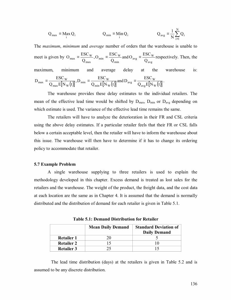
136
ii
max QMaxQ = ii
min QMinQ = ∑=
=N
1iiavg Q
N1Q
The maximum, minimum and average number of orders that the warehouse is unable to
meet is given by avg
Wavg
min
Wmin
max
Wmax Q
ESCOand
QESC
O,Q
ESCO === respectively. Then, the
maximum, minimum and average delay at the warehouse is:
( )[ ] ( )[ ] ( )[ ]tNEQESC
DandtNEQ
ESCD,
tNEQESC
DWavg
Wavg
Wmin
Wmin
Wmax
Wmax === .
The warehouse provides these delay estimates to the individual retailers. The
mean of the effective lead time would be shifted by Dmax, Dmin or Davg depending on
which estimate is used. The variance of the effective lead time remains the same.
The retailers will have to analyze the deterioration in their FR and CSL criteria
using the above delay estimates. If a particular retailer feels that their FR or CSL falls
below a certain acceptable level, then the retailer will have to inform the warehouse about
this issue. The warehouse will then have to determine if it has to change its ordering
policy to accommodate that retailer.
5.7 Example Problem
A single warehouse supplying to three retailers is used to explain the
methodology developed in this chapter. Excess demand is treated as lost sales for the
retailers and the warehouse. The weight of the product, the freight data, and the cost data
at each location are the same as in Chapter 4. It is assumed that the demand is normally
distributed and the distribution of demand for each retailer is given in Table 5.1.
Table 5.1: Demand Distribution for Retailer
Mean Daily Demand Standard Deviation of Daily Demand
Retailer 1 20 5 Retailer 2 15 10 Retailer 3 25 15
The lead time distribution (days) at the retailers is given in Table 5.2 and is
assumed to be any discrete distribution.
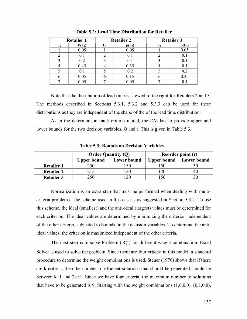
137
Table 5.2: Lead Time Distribution for Retailer
Retailer 1 Retailer 2 Retailer 3 L1 P(L1) L2 p(L2) L3 p(L3) 1 0.05 1 0.05 1 0.05 2 0.1 2 0.1 2 0.1 3 0.2 3 0.1 3 0.1 4 0.45 4 0.35 4 0.1 5 0.1 5 0.2 5 0.2 6 0.05 6 0.15 6 0.35 7 0.05 7 0.05 7 0.1
Note that the distribution of lead time is skewed to the right for Retailers 2 and 3.
The methods described in Sections 5.3.1, 5.3.2 and 5.3.3 can be used for these
distributions as they are independent of the shape of the of the lead time distribution.
As in the deterministic multi-criteria model, the DM has to provide upper and
lower bounds for the two decision variables, Q and r. This is given in Table 5.3.
Table 5.3: Bounds on Decision Variables
Order Quantity (Q) Reorder point (r) Upper bound Lower bound Upper bound Lower bound
Retailer 1 250 150 150 30 Retailer 2 215 120 120 40 Retailer 3 250 130 150 30
Normalization is an extra step that must be performed when dealing with multi-
criteria problems. The scheme used in this case is as suggested in Section 5.3.2. To use
this scheme, the ideal (smallest) and the anti-ideal (largest) values must be determined for
each criterion. The ideal values are determined by minimizing the criterion independent
of the other criteria, subjected to bounds on the decision variables. To determine the anti-
ideal values, the criterion is maximized independent of the other criteria.
The next step is to solve Problem ( λiR ) for different weight combination. Excel
Solver is used to solve the problem. Since there are four criteria in this model, a standard
procedure to determine the weight combinations is used. Steuer (1976) shows that if there
are k criteria, then the number of efficient solutions that should be generated should lie
between k+1 and 2k+1. Since we have four criteria, the maximum number of solutions
that have to be generated is 9. Starting with the weight combinations (1,0,0,0), (0,1,0,0),

138
(0,0,1,0) and (0,0,0,1), the fifth weight combination is determined by calculating the
centroid as (1/4,1/4,1/4,1/4). Using any three of the initial weight combinations and the
fifth weight combination, the other four weight combinations are determined. For
example, the sixth weight combination is the centroid of (1,0,0,0), (0,1,0,0), (0,0,1,0) and
(1/4,1/4,1/4,1/4) which is (5/16,5/16,5/16,1/16). The rest of the weight combinations are
given in Table 5.4. The Pλ problem can now be solved for each retailer for the weight
combinations given in Table 5.4.
Note: Instead of choosing some weight combinations, one could interact with the
decision maker and get the preference information on the criteria by different methods.
This approach is illustrated in the case study discussed in Chapter 6.
Table 5.4: Weight Combinations
Weight Combinations Weights 1 (1,0,0,0) 2 (0,1,0,0) 3 (0,0,1,0) 4 (0,0,0,1) 5 (1/4, 1/4, 1/4, 1/4) 6 (5/16, 5/16, 5/16, 1/16) 7 (5/16, 5/16, 1/16, 5/16) 8 (5/16, 1/16, 5/16, 5/16) 9 (1/16, 5/16, 5/16, 5/16)
We know from Section 5.3.3 that the conditional distribution of LTD for each
retailer is ( )2DiDi j,jN σµ . Hence, ESC and safety stock can be calculated. Sample
calculations for Retailer 1 for weight combination (5/16,1/16,5/16,5/16) is tabulated in
Table 5.5. The values of Q and r after optimization are 250 and 81.12 units.

139
Table 5.5: Sample Calculations
L1 p(L1) Dijµ Dijσ
Di
Di
j)jr(
σµ− ESC|j s|j
1 0.05 20 5 12.2331 0 61.1654 2 0.1 40 7.0711 5.8217 0 41.1654 3 0.2 60 8.6603 2.4440 0.0206 21.1860 4 0.45 80 10 0.1165 3.4338 4.5992 5 0.1 100 11.1803 -1.6846 19.0469 0.2123 6 0.05 120 12.2474 -3.1708 38.8372 0.0025 7 0.05 140 13.2288 -4.4475 58.8346 0
The first two columns of Table 5.5 represent the lead time distribution. The third and
fourth columns are the conditional mean and standard deviation of demand during period
j, respectively. The conditional ESC for lead time of 4 days is computed using:
( )
σµ−−−µ+σ
σµ−
=1D
1D1j1LD11D1D
1D
1D1j1LD
j1 j
jrF1rjjjjr
fESC (see Eq. 5.46)
The above formula is calculated in Excel as:
NORMDIST(0.1165,0,1,0)*10+(80-81.12)*(1-NORMDIST(0.1165,0,1,1))=3.4338 units.
The conditional ESC for all possible values of the lead time is computed. The
total ESC for Retailer 1 for the weight combination (5/16,1/16,5/16,5/16)
is 3376.805.0*8346.58...1.0*005.0*0pESCESC j1
j
j11 =+++==∑ units.
The conditional safety stock for Retailer 1 is calculated using j11D1
j1 ESCjrs +µ−= (see Eq. 5.21). These values are given in the last column of Table
5.5. The total safety stock for Retailer 1 is:
503.1305.0*0...1.0*1654.4105.0*1654.61pss j1
j
j11 =+++==∑ units.
The output of the Pλ problem is given in Table 5.6. The normalized criterion
values are given in Table 5.7. The value path approach described in Chapter 4 is used to
present the DM with the set of efficient solutions. This is shown in Fig. 5.2. If the DM is
not satisfied with the current set of solutions, another set of solutions can be generated by
tweaking the values of the weight parameters.

140
T
able
5.6
: Cri
teri
a V
alue
s fo
r th
e R
etai
lers
R
etai
ler
1 R
etai
ler
2 R
etai
ler
3 W
eigh
t C
ombi
natio
n C
rite
rion
1 C
rite
rion
2 C
rite
rion
3 C
rite
rion
4 C
rite
rion
1 C
rite
rion
2 C
rite
rion
3 C
rite
rion
4 C
rite
rion
1 C
rite
rion
2 C
rite
rion
3 C
rite
rion
4
1 65
73.5
59
56.1
5385
24
092.
90
0.35
7903
89
34.7
64
45.6
25
1858
0.67
0.
2220
59
9903
.496
70
.19
2398
0.3
0.68
8061
2
1257
3.56
29
.2
1918
4.24
0.
1861
09
1558
4.76
25
.465
12
1516
4.45
0.
1239
4 18
903.
5 36
.5
2398
0.3
0.35
7792
3
1257
3.56
29
.2
1918
4.24
0.
1861
09
1558
4.76
25
.465
12
1516
4.45
0.
1239
4 18
903.
5 36
.5
2398
0.3
0.35
7792
4
1992
9.55
29
.2
1918
4.24
0.
0003
49
2312
0.06
25
.465
12
1516
4.45
0.
0021
89
2486
8.65
36
.5
2398
0.3
0.03
6863
5
1387
1.12
29
.2
1918
4.24
0.
0333
5 17
908.
11
25.4
6512
15
164.
45
0.03
095
2109
3.11
36
.5
2398
0.3
0.12
3619
6
1292
7.82
29
.2
1918
4.24
0.
0910
62
1581
0.52
25
.465
12
1516
4.45
0.
1033
43
1910
1.68
36
.5
2398
0.3
0.29
7801
7
1387
1.12
29
.2
1918
4.24
0.
0333
5 17
908.
11
25.4
6512
15
164.
45
0.03
095
2109
3.11
36
.5
2398
0.3
0.12
3619
8
1387
1.12
29
.2
1918
4.24
0.
0333
5 17
908.
11
25.4
6512
15
164.
45
0.03
095
2109
3.11
36
.5
2398
0.3
0.12
3619
9
1592
5.63
29
.2
1918
4.24
0.
0098
49
2120
9.5
25.4
6512
15
164.
45
0.00
6076
24
868.
65
36.5
23
980.
3 0.
0368
63
Idea
l 65
73.5
6 29
.2
1918
4.24
0.
0003
49
8934
.764
25
.465
12
1516
4.45
0.
0021
89
9903
.496
36
.5
2398
0.3
0.03
6863
A
nti-I
deal
19
929.
55
56.1
5385
24
092.
90
0.35
7903
23
120.
0559
45
.625
18
580.
67
0.22
2059
24
868.
65
70.1
9 30
116.
12
0.68
8061
Tab
le 5
.7: N
orm
aliz
ed C
rite
ria
Val
ues f
or th
e R
etai
lers
R
etai
ler
1 R
etai
ler
2 R
etai
ler
3 W
eigh
t C
ombi
natio
n C
rite
rion
1 C
rite
rion
2 C
rite
rion
3 C
rite
rion
4 C
rite
rion
1 C
rite
rion
2 C
rite
rion
3 C
rite
rion
4 C
rite
rion
1 C
rite
rion
2 C
rite
rion
3 C
rite
rion
4
1 0
1 1
1 0
1 1
1 0
1 1
1 2
0.44
92
0 0
0.51
95
0.46
88
0 0
0.55
37
0.60
14
0 0
0.49
28
3 0.
4492
0
0 0.
5195
0.
4688
0
0 0.
5537
0.
6014
0
0 0.
4928
4
1.00
00
0 0
0.00
00
1.00
00
0 0
0.00
00
1.00
00
0 0
0.00
00
5 0.
5464
0
0 0.
0923
0.
6326
0
0 0.
1308
0.
7477
0
0 0.
1332
6
0.47
58
0 0
0.25
37
0.48
47
0 0
0.46
01
0.61
46
0 0
0.40
07
7 0.
5464
0
0 0.
0923
0.
6326
0
0 0.
1308
0.
7477
0
0 0.
1332
8
0.54
64
0 0
0.09
23
0.63
26
0 0
0.13
08
0.74
77
0 0
0.13
32
9 0.
7002
0
0 0.
0266
0.
8653
0
0 0.
0177
1.
0000
0
0 0.
0000
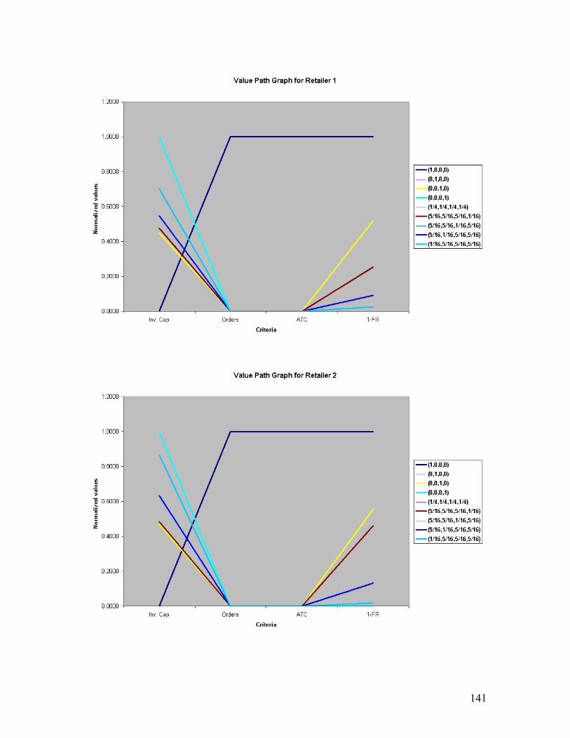
141

142
Fig. 5.2: Value Path Graphs for Retailers
A tradeoff analysis can be used to validate the results obtained from the
optimization models. For example, for Retailer 1, consider weight combinations 4
(1/4,1/4,1/4,1/4) and 5 (5/16,5/16,5/16,1/16). The capital invested in inventory decreases
by 30.4%, and fill rate increases by 94.56%, while the other two criteria remain
unchanged. This is because the DM�s preference for capital invested in inventory,
number of orders, and transportation costs has increased, while his/her�s preference
towards fill rate has reduced.
Recall that )r(F iLDi is the cycle service level for each retailer. It can be used as
another measure of customer satisfaction. To capture how CSL and FR behave, we first
vary the weight of the fill rate criterion, λ4, and annual transportation costs, λ3, while
keeping the weights of capital invested in inventory, λ1, and annual number of orders
placed, λ2, constant at 0.025. This is shown in Fig. 5.3a. The alternatives in the X axis
refer to a particular combination of (λ3,λ4), e.g., alternative 1 is (0.05,0.9), alternative 2 is
(0.1,0.85), etc. In Fig. 5.3b, λ2 and λ3 kept constant at 0.025 while (λ1,λ4) are varied.
143
Fig. 5.3a and b: Behavior of Fill Rate/Cycle Service Level

144
As we move across the right in Fig. 5.3a (λ3 increases, λ4 decreases), the CSL
starts to decreases while the FR is almost constant. This is because the FR is primarily
influenced by the value of Q, which increases as λ3 increases. CSL is only influenced by
the value of r and starts to decrease as λ4 decreases. In Fig. 5.3a, the FR is 97.82% for
(λ3,λ4) = (0.9, 0.05), while CSL is 74.93%.
As we move across the right in Fig. 5.3b (λ1 increases, λ4 decreases) both the FR
and CSL decreases; however, the decrease in CSL is significant. For example, for (λ1,λ4)
= (0.9,0.05), the FR is 75.04% while the CSL is 13.77%. Thus, in addition to looking at
the 4 criteria, the DM must also observe CSL, as in some cases even when the FR is
acceptable, the CSL may be unsatisfactory.
To determine the most preferred solution, the DM has to use Table 5.7 and Fig.
5.2 to analyze the tradeoff information. Observing the values in Table 5.7, the annual
number of orders placed and the annual transportation costs takes only two values, the
ideal and anti-ideal, for all the retailers. Capital invested in inventory is minimized when
Q and r are fixed at their lower bounds. The annual number of orders and annual
transportation costs are minimized when Q is fixed at the upper bound. FR is maximized
(1-FR is minimized) when Q and r at their upper bounds. Since 3 out of the 4 criteria are
minimized for larger values of Q, care should be taken while setting the value of λ1 so
that the capital invested in inventory criterion does not get dominated. Taking this and the
CSL into account the retailers� ordering policies are given in Table 5.8. The criteria
values are given in Table 5.9.
Table 5.8: Ordering Policy for the Retailers
Weights Order Quantity Reorder point
Retailer 1 (0.4,0.05,0.15,0.4) 213.16 83.16 Retailer 2 (0.45,0.05,0.2,0.3) 200.54 70.21 Retailer 3 (0.3,0.05,0.1,0.55) 189.8 135.12
Table 5.9: Most Preferred Criteria Values for the Retailers
Capital Invested in Inventory
Annual Number of Orders
Annual Transportation Cost
Fill Rate
Retailer 1 $12152.37 34.25 $20279.82 96.45% Retailer 2 $16321.3 27.30 $15536.78 95.55% Retailer 3 $18911.09 48.08 $26396.12 92.41%
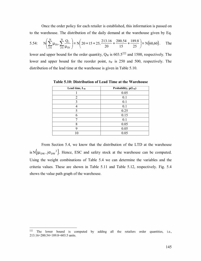
145
Once the order policy for each retailer is established, this information is passed on
to the warehouse. The distribution of the daily demand at the warehouse given by Eq.
5.54: ( )60,60N25
8.18915
54.20020
16.213,251520NQ
,NN
1i Di
iN
1iDi =
++++=
µµ ∑∑
==. The
lower and upper bound for the order quantity, QW is 603.5��� and 1500, respectively. The
lower and upper bound for the reorder point, rW is 250 and 500, respectively. The
distribution of the lead time at the warehouse is given in Table 5.10.
Table 5.10: Distribution of Lead Time at the Warehouse Lead time, LW Probability, p(LW)
1 0.05 2 0.1 3 0.1 4 0.1 5 0.25 6 0.15 7 0.1 8 0.05 9 0.05 10 0.05
From Section 5.4, we know that the distribution of the LTD at the warehouse
is ( )2DWDW j,jN σµ . Hence, ESC and safety stock at the warehouse can be computed.
Using the weight combinations of Table 5.4 we can determine the variables and the
criteria values. These are shown in Table 5.11 and Table 5.12, respectively. Fig. 5.4
shows the value path graph of the warehouse.
��� The lower bound is computed by adding all the retailers order quantities, i.e., 213.16+200.54+189.8=603.5 units.
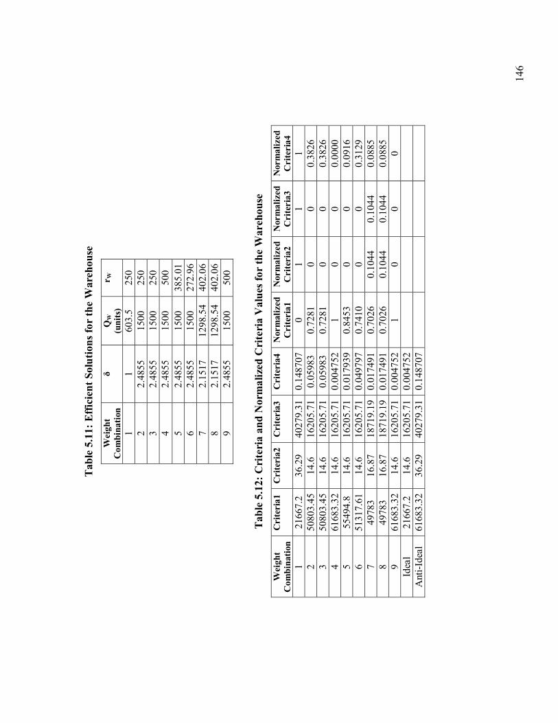
146
Tab
le 5
.11:
Effi
cien
t Sol
utio
ns fo
r th
e W
areh
ouse
W
eigh
t C
ombi
natio
n δ
QW
(u
nits
) r W
1 1
603.
5 25
0 2
2.48
55
1500
25
0 3
2.48
55
1500
25
0 4
2.48
55
1500
50
0 5
2.48
55
1500
38
5.01
6 2.
4855
15
00
272.
967
2.15
17
1298
.54
402.
068
2.15
17
1298
.54
402.
069
2.48
55
1500
50
0
Tab
le 5
.12:
Cri
teri
a an
d N
orm
aliz
ed C
rite
ria
Val
ues f
or th
e W
areh
ouse
W
eigh
t C
ombi
natio
n C
rite
ria1
C
rite
ria2
C
rite
ria3
C
rite
ria4
N
orm
aliz
ed
Cri
teri
a1
Nor
mal
ized
C
rite
ria2
N
orm
aliz
ed
Cri
teri
a3
Nor
mal
ized
C
rite
ria4
1
2166
7.2
36.2
9 40
279.
31
0.14
8707
0
1 1
1 2
5080
3.45
14
.6
1620
5.71
0.
0598
3 0.
7281
0
0 0.
3826
3
5080
3.45
14
.6
1620
5.71
0.
0598
3 0.
7281
0
0 0.
3826
4
6168
3.32
14
.6
1620
5.71
0.
0047
52
1 0
0 0.
0000
5
5549
4.8
14.6
16
205.
71
0.01
7939
0.
8453
0
0 0.
0916
6
5131
7.61
14
.6
1620
5.71
0.
0497
97
0.74
10
0 0
0.31
29
7 49
783
16.8
7 18
719.
19
0.01
7491
0.
7026
0.
1044
0.
1044
0.
0885
8
4978
3 16
.87
1871
9.19
0.
0174
91
0.70
26
0.10
44
0.10
44
0.08
85
9 61
683.
32
14.6
16
205.
71
0.00
4752
1
0 0
0 Id
eal
2166
7.2
14.6
16
205.
71
0.00
4752
A
nti-I
deal
61
683.
32
36.2
9 40
279.
31
0.14
8707
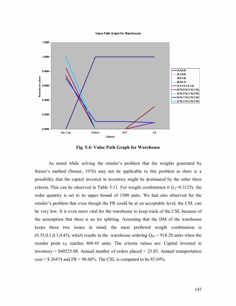
147
Fig. 5.4: Value Path Graph for Warehouse
As noted while solving the retailer�s problem that the weights generated by
Steuer�s method (Steuer, 1976) may not be applicable to this problem as there is a
possibility that the capital invested in inventory might be dominated by the other three
criteria. This can be observed in Table 5.11. For weight combination 6 (λ1=0.3125), the
order quantity is set to its upper bound of 1500 units. We had also observed for the
retailer�s problem that even though the FR could be at an acceptable level, the CSL can
be very low. It is even more vital for the warehouse to keep track of the CSL because of
the assumption that there is no lot splitting. Assuming that the DM of the warehouse
keeps these two issues in mind, the most preferred weight combination is
(0.35,0.1,0.1,0.45), which results in the warehouse ordering QW = 918.20 units when the
reorder point rW reaches 460.45 units. The criteria values are: Capital invested in
inventory = $40525.08, Annual number of orders placed = 23.85, Annual transportation
cost = $ 26474 and FR = 98.68%. The CSL is computed to be 85.69%.

148
5.8 Summary
In this chapter we modeled and solved the inventory problem for a decentralized
single warehouse multi-retailer system with transportation costs using a multi-criteria
approach when demand and lead time are treated as random variables. The retailers face
independent but non-identical demands. Three distributions of external demand were
considered: Poisson, geometric Poisson, and normal. The lead times were assumed to
follow any general discrete distribution. The demand at the warehouse was approximated
using a normal distribution based on renewal theory. Fill rate was used to measure the
customer service at each location. Both the lost sales and backorders case were
considered. The weighted objective method was used with the value path method to help
the DM choose the most preferred solution. An example problem was used to explain the
methodology developed.
In the next chapter, the results obtained by applying the models developed in
Chapters 3, 4 and 5 to real world data obtained from a Fortune 500 consumer products
company are discussed.
149
Chapter 6
CASE STUDIES
6.1 Introduction
The purpose in this chapter is to validate the theoretical models developed in the
previous chapters by applying them to inventory planning case studies for a product
manufactured by a Fortune 500 consumer products company. It is well known that there
is a gap between the theoretical models and real world problems. While some models
may not represent situations faced in practice, others may be too complicated for practical
implementation. This chapter bridges that gap. After explaining the details of the case,
the problems are solved under the model assumptions given in Chapters 3, 4 and 5, and
their results are discussed. Also, some of the practical problems faced while using these
models with the real world data and their resolutions are also discussed. Implementation
is done using Microsoft Excel, which is widely available.
6.2 Case Study Description
The case study deals with planning the inventory for a functional product
manufactured by a Fortune 500 company with a relatively stable demand. The company
wants to manage its inventory for a one year period (tactical planning) so that it can serve
up to 20 retailers. Daily sales data for the past three years are available. Since the
company operates at high service levels, the demand can be approximated by the sales
data. The cost of the product at the warehouse, CW=$19.10/box. The selling price of the
product (cost at the retailer), Ci is roughly§§§ $21/box assuming FOB origin. The weight
of a box of the product (ω) is 40 lbs. The lead times for the retailer and the warehouse are
in the interval [1,3] days.
6.3 Case Study 1: Chapter 3
6.3.1 Overview
The purpose of this study is to test the effectiveness of the modified base period
policy developed using a single objective cost (sum of inventory holding costs and
§§§ The differences in the selling prices among the retailers are not significant as the product is functional.

150
ordering costs) framework to this data. The closed-form expressions are coded using
Visual Basic (VB) macros in Excel. The demand estimate for the current year was
obtained by taking the average of the last three years data. The exact marginal cost
information, i.e., the ordering and opportunity costs at each retailer and warehouse
location were not available. The ordering cost was assumed to be ai = $50 and aW = $40.
The opportunity cost at each location was assumed to be Ii = IW =0.17/$/year. Thus, the
inventory holding costs are computed as hi = IiCi =$3.6992/unit/year and hW = IWCW
=$3.247/unit/year.
6.3.2 Results
The above information was input into Excel. The optimal results (order quantity,
time between orders and annual inventory cost) for each retailer after solving the EOQ
problem are as shown in Table 6.1.
Table 6.1: Output of EOQ Problem for Retailers
Retailers Demand Q*(units) T*(weeks) Z*($) 1 17102 679.94 2.0674 2515.23 2 15416 645.55 2.1775 2388.03 3 20736 748.70 1.8775 2769.60 4 47185 1129.40 1.2447 4177.88 5 5091 370.98 3.7892 1372.32 6 6648 423.93 3.3159 1568.19 7 8931 491.36 2.8609 1817.62 8 34027 959.09 1.4657 3547.85 9 64727 1322.78 1.0627 4893.24 10 38213 1016.37 1.3831 3759.75 11 6847 430.23 3.2674 1591.49 12 41243 1055.90 1.3313 3905.97 13 7210 441.48 3.1841 1633.13 14 29806 897.63 1.5660 3320.52 15 25036 822.68 1.7087 3043.24 16 8809 487.99 2.8806 1805.17 17 14274 621.18 2.2630 2297.88 18 51589 1180.93 1.1903 4368.50 19 9831 515.52 2.7268 1907.01 20 19002 716.71 1.9613 2651.27
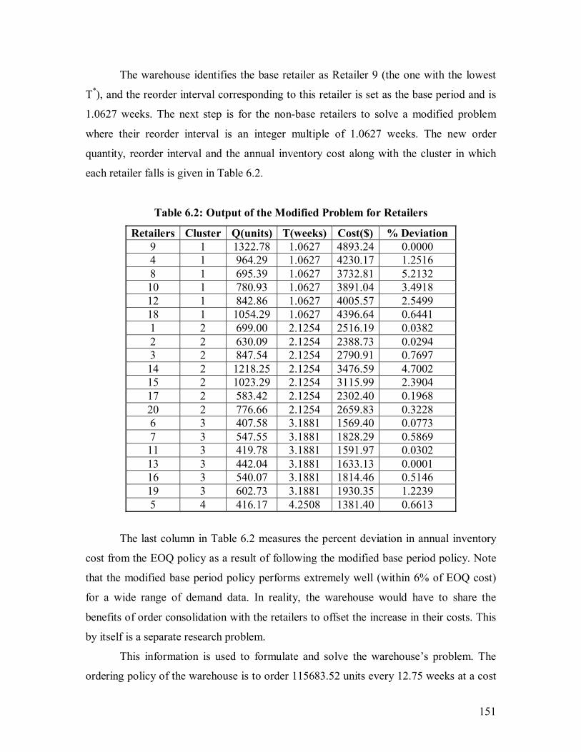
151
The warehouse identifies the base retailer as Retailer 9 (the one with the lowest
T*), and the reorder interval corresponding to this retailer is set as the base period and is
1.0627 weeks. The next step is for the non-base retailers to solve a modified problem
where their reorder interval is an integer multiple of 1.0627 weeks. The new order
quantity, reorder interval and the annual inventory cost along with the cluster in which
each retailer falls is given in Table 6.2.
Table 6.2: Output of the Modified Problem for Retailers
Retailers Cluster Q(units) T(weeks) Cost($) % Deviation 9 1 1322.78 1.0627 4893.24 0.0000 4 1 964.29 1.0627 4230.17 1.2516 8 1 695.39 1.0627 3732.81 5.2132 10 1 780.93 1.0627 3891.04 3.4918 12 1 842.86 1.0627 4005.57 2.5499 18 1 1054.29 1.0627 4396.64 0.6441 1 2 699.00 2.1254 2516.19 0.0382 2 2 630.09 2.1254 2388.73 0.0294 3 2 847.54 2.1254 2790.91 0.7697 14 2 1218.25 2.1254 3476.59 4.7002 15 2 1023.29 2.1254 3115.99 2.3904 17 2 583.42 2.1254 2302.40 0.1968 20 2 776.66 2.1254 2659.83 0.3228 6 3 407.58 3.1881 1569.40 0.0773 7 3 547.55 3.1881 1828.29 0.5869 11 3 419.78 3.1881 1591.97 0.0302 13 3 442.04 3.1881 1633.13 0.0001 16 3 540.07 3.1881 1814.46 0.5146 19 3 602.73 3.1881 1930.35 1.2239 5 4 416.17 4.2508 1381.40 0.6613
The last column in Table 6.2 measures the percent deviation in annual inventory
cost from the EOQ policy as a result of following the modified base period policy. Note
that the modified base period policy performs extremely well (within 6% of EOQ cost)
for a wide range of demand data. In reality, the warehouse would have to share the
benefits of order consolidation with the retailers to offset the increase in their costs. This
by itself is a separate research problem.
This information is used to formulate and solve the warehouse�s problem. The
ordering policy of the warehouse is to order 115683.52 units every 12.75 weeks at a cost
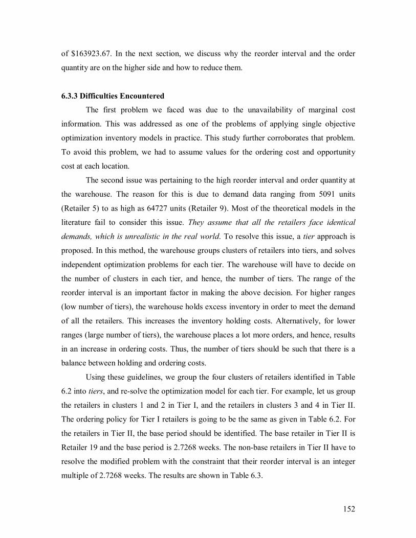
152
of $163923.67. In the next section, we discuss why the reorder interval and the order
quantity are on the higher side and how to reduce them.
6.3.3 Difficulties Encountered
The first problem we faced was due to the unavailability of marginal cost
information. This was addressed as one of the problems of applying single objective
optimization inventory models in practice. This study further corroborates that problem.
To avoid this problem, we had to assume values for the ordering cost and opportunity
cost at each location.
The second issue was pertaining to the high reorder interval and order quantity at
the warehouse. The reason for this is due to demand data ranging from 5091 units
(Retailer 5) to as high as 64727 units (Retailer 9). Most of the theoretical models in the
literature fail to consider this issue. They assume that all the retailers face identical
demands, which is unrealistic in the real world. To resolve this issue, a tier approach is
proposed. In this method, the warehouse groups clusters of retailers into tiers, and solves
independent optimization problems for each tier. The warehouse will have to decide on
the number of clusters in each tier, and hence, the number of tiers. The range of the
reorder interval is an important factor in making the above decision. For higher ranges
(low number of tiers), the warehouse holds excess inventory in order to meet the demand
of all the retailers. This increases the inventory holding costs. Alternatively, for lower
ranges (large number of tiers), the warehouse places a lot more orders, and hence, results
in an increase in ordering costs. Thus, the number of tiers should be such that there is a
balance between holding and ordering costs.
Using these guidelines, we group the four clusters of retailers identified in Table
6.2 into tiers, and re-solve the optimization model for each tier. For example, let us group
the retailers in clusters 1 and 2 in Tier I, and the retailers in clusters 3 and 4 in Tier II.
The ordering policy for Tier I retailers is going to be the same as given in Table 6.2. For
the retailers in Tier II, the base period should be identified. The base retailer in Tier II is
Retailer 19 and the base period is 2.7268 weeks. The non-base retailers in Tier II have to
resolve the modified problem with the constraint that their reorder interval is an integer
multiple of 2.7268 weeks. The results are shown in Table 6.3.

153
Table 6.3: Output of the Modified Problem for Retailers in Tier II
Retailers Cluster Q(units) T(weeks) Cost($) % Deviation 19 1 515.52 2. 7268 1907.01 0.00 5 1 266.96 2.7268 1447.28 5.4622 6 1 348.6087 2. 7268 1598.291 1.9193 7 1 468.325 2. 7268 1819.718 0.1153 11 1 359.0439 2. 7268 1617.592 1.6401 13 1 378.08 2. 7268 1652.80 1.2042 16 1 461.93 2. 7268 1807.89 0.1506
All the retailers in Tier II are classified in once cluster. Again, the percent
deviation in cost as a result of following the modified base period policy is less than 6%.
The warehouse has to solve its optimization problems for Tier I and Tier II
separately. The result after solving these two optimization problems along with the result
without using the tier approach is shown in Table 6.4.
Table 6.4: Comparison of Results with and without Tiered Approach
Tier approach Without Tier approach Tier I Tier II
Order Quantity (units) 115,683.52 17099.34 2798.47 Reorder Interval (weeks) 12.75 2.1254 2.7268
Annual Costs ($) 163,923.67 10,168.54 762.8
The total annual cost at the warehouse using the tier approach is $10931.14 way
below $163923.67, the cost when the warehouse�s problem was solved in a single step, a
decrease of 93.33 %. This enormous decrease is attributed to the reduction in the reorder
interval and hence, reduction in inventory holding costs.
6.4 Case Study 2: Chapter 4
6.4.1 Overview
In this study we would like to demonstrate the usefulness of a multi-criteria
approach to determine the ordering policies for the companies in the supply chain when
transportation costs are considered between the echelons. The three criteria used in the
model formulation are capital invested in inventory, annual number of orders, and annual
transportation costs. FOB origin is assumed. Since the problem is formulated as a multi-

154
criteria problem, we do not have to make any assumptions about opportunity and
ordering costs as in the previous case study. We use the same freight rate data as in
Chapter 4 and Chapter 5. Based on that data, the cost of a full TL is $1110. A truck can
carry up to 46,000 lbs (460 cwt). Hence, TL rate is 1110/460 = $2.413/cwt. The retailer
shipments are modeled using a power function while the warehouse�s shipments are
modeled using an inverse function. The lead times of the retailers are in the interval [1,3]
days. The lead time of the warehouse is 3 days. The demand estimates are the same as in
the previous study. To simulate the decision making process, we used an executive from
the same Fortune 500 company to specify the upper and lower bounds on the order
quantity and provide preference information pertaining to the three criteria using three
different methods (discussed in the next section). Using this preference information, three
sets of weights for the criteria were computed. These weights were used in the model to
obtain efficient solutions from which the DM could analyze the tradeoffs and choose the
most preferred solution. Excel Solver and VB macros were used to generate efficient
solutions.
6.4.2 Results
Each retailer starts off by solving Problem (Ri) by inputting different weight
combinations. Assuming that the DM has chosen the most preferred solution, the
ordering policy for the retailers is given in Table 6.5.
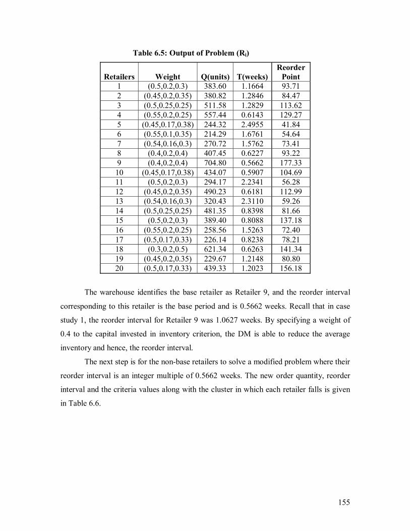
155
Table 6.5: Output of Problem (Ri)
Retailers Weight Q(units) T(weeks)Reorder
Point 1 (0.5,0.2,0.3) 383.60 1.1664 93.71 2 (0.45,0.2,0.35) 380.82 1.2846 84.47 3 (0.5,0.25,0.25) 511.58 1.2829 113.62 4 (0.55,0.2,0.25) 557.44 0.6143 129.27 5 (0.45,0.17,0.38) 244.32 2.4955 41.84 6 (0.55,0.1,0.35) 214.29 1.6761 54.64 7 (0.54,0.16,0.3) 270.72 1.5762 73.41 8 (0.4,0.2,0.4) 407.45 0.6227 93.22 9 (0.4,0.2,0.4) 704.80 0.5662 177.33 10 (0.45,0.17,0.38) 434.07 0.5907 104.69 11 (0.5,0.2,0.3) 294.17 2.2341 56.28 12 (0.45,0.2,0.35) 490.23 0.6181 112.99 13 (0.54,0.16,0.3) 320.43 2.3110 59.26 14 (0.5,0.25,0.25) 481.35 0.8398 81.66 15 (0.5,0.2,0.3) 389.40 0.8088 137.18 16 (0.55,0.2,0.25) 258.56 1.5263 72.40 17 (0.5,0.17,0.33) 226.14 0.8238 78.21 18 (0.3,0.2,0.5) 621.34 0.6263 141.34 19 (0.45,0.2,0.35) 229.67 1.2148 80.80 20 (0.5,0.17,0.33) 439.33 1.2023 156.18
The warehouse identifies the base retailer as Retailer 9, and the reorder interval
corresponding to this retailer is the base period and is 0.5662 weeks. Recall that in case
study 1, the reorder interval for Retailer 9 was 1.0627 weeks. By specifying a weight of
0.4 to the capital invested in inventory criterion, the DM is able to reduce the average
inventory and hence, the reorder interval.
The next step is for the non-base retailers to solve a modified problem where their
reorder interval is an integer multiple of 0.5662 weeks. The new order quantity, reorder
interval and the criteria values along with the cluster in which each retailer falls is given
in Table 6.6.
156
Table 6.6: Output of the Modified Problem for Retailers
Retailers Cluster Q(units) T(weeks)
Capital invested in
inventory($)
Annual number of
orders
Annual Transportation
costs($) 9 1 704.80 0.5662 11527.04 91.84 118544.90 10 1 416.10 0.5662 6805.24 91.84 84090.77 8 1 370.51 0.5662 6059.77 91.84 77967.91 18 1 561.74 0.5662 9187.34 91.84 102254.35 4 1 513.79 0.5662 8403.04 91.84 96478.43 12 1 449.09 0.5662 7344.85 91.84 88377.52 1 2 372.44 1.1324 6091.29 45.92 39115.97 2 2 335.72 1.1324 5490.78 45.92 36558.06 3 2 451.58 1.1324 7385.63 45.92 44348.48 14 2 649.11 1.1324 8839.20 45.92 56176.80 15 2 545.23 1.1324 8917.18 45.92 50142.46 17 2 310.85 1.1324 5084.03 45.92 34769.84 19 2 214.10 1.1324 4087.64 45.92 27269.51 20 2 413.82 1.1324 7900.85 45.92 41895.40 6 3 217.17 1.6987 3551.77 30.61 18349.15 7 3 291.74 1.6987 4771.49 30.61 22241.14 16 3 287.76 1.6987 4706.31 30.61 22042.70 5 4 221.74 2.2649 3323.06 22.96 13950.02 11 4 298.22 2.2649 4469.26 22.96 16921.31 13 4 314.03 2.2649 4706.20 22.96 17500.58
Using the information of Table 6.6, the warehouse formulates and solves its
multi-criteria optimization problem. For the retailers, we had assumed a weight
combination as the most preferred combination. However, for the warehouse we were
able to obtain the preference information of the DM (the company executive) using the
following methods.
Method 1 (Rating method):
In this method the DM is asked to rate the criteria on a 1-10 scale where 1
indicates a low score and 10 indicates a high score. Then the weights can be computed as
shown in Table 6.7.

157
Table 6.7: Weights Using Method 1
Criteria Score (1-10) Weights Capital invested in inventory 7 7/15=0.47
Annual number of orders 3 3/15=0.2 Annual transportation costs 5 5/15=0.33
Total 15
Method 2 (Pairwise Comparison method):
In this method the DM is asked questions about his preference with respect to a
pair of criteria. Let { }ijaA = be the pairwise comparison matrix (Ravindran, 2003). Then
we have the following:
iaii ∀= 1
If ji f then 0,1 == jiij aa If ij f then 0,1 == ijji aa
If ji ⇔ then 1== jiij aa
where: f - More preference
⇔ - Equal preference
Using these guidelines, the parirwise comparison matrix was obtained from the company
executive and the weights were computed as shown in Table 6.8.
Table 6.8: Weights Using Method 2
Capital invested in inventory
Annual number of orders
Annual transportation
costs Total Weights Capital invested in
inventory 1 1 1 3 3/6=0.5 Annual number of orders 0 1 0 1 1/6=0.17
Annual transportation costs 0 1 1 2 2/6=0.33 6
Method 3:
It is an extension of the pairwise comparison method and is used in the Analytical
Hierarchy Process (Saaty, 1980). In this method the DM has to indicate the strength of
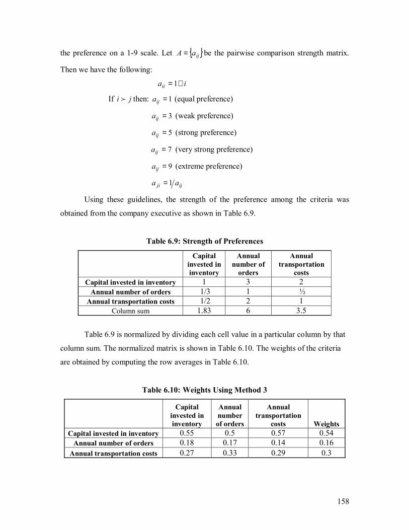
158
the preference on a 1-9 scale. Let { }ijaA = be the pairwise comparison strength matrix.
Then we have the following:
iaii ∀= 1
If ji f then: 1=ija (equal preference)
3=ija (weak preference)
5=ija (strong preference) 7=ija (very strong preference)
9=ija (extreme preference)
ijji aa 1=
Using these guidelines, the strength of the preference among the criteria was
obtained from the company executive as shown in Table 6.9.
Table 6.9: Strength of Preferences
Capital invested in inventory
Annual number of
orders
Annual transportation
costs Capital invested in inventory 1 3 2
Annual number of orders 1/3 1 ½ Annual transportation costs 1/2 2 1
Column sum 1.83 6 3.5
Table 6.9 is normalized by dividing each cell value in a particular column by that
column sum. The normalized matrix is shown in Table 6.10. The weights of the criteria
are obtained by computing the row averages in Table 6.10.
Table 6.10: Weights Using Method 3
Capital invested in inventory
Annual number of orders
Annual transportation
costs Weights Capital invested in inventory 0.55 0.5 0.57 0.54
Annual number of orders 0.18 0.17 0.14 0.16 Annual transportation costs 0.27 0.33 0.29 0.3

159
The weight combinations that best described the company executive�s preference
by the three methods were (0.47,0.2,0.33), (0.5,0.17,0.33) and (0.54,0.16,0.3). The
efficient solutions for the warehouse are given in Table 6.11. Since the ordering policy is
the same for the three weight combinations, we decided to generate two extreme efficient
solutions, i.e., one that minimizes capital invested in inventory, and the other that
minimizes annual transportation costs.
Table 6.11: Efficient Solutions for the Warehouse
Weight QW TW(weeks) Criterion1($) Criterion2 Criterion3($)(0.47,0.2,0.33) 123276.47 13.59 1175521.57 3.83 4247.39 (0.5,0.17,0.33) 123276.47 13.59 1175521.57 3.83 4247.39 (0.54,0.16,0.3) 123276.47 13.59 1175521.57 3.83 4247.39 (0.7,0.1,0.2) 61638.24 6.79 586876.41 7.65 8494.78
(0.35,0.2,0.45) 184914.71 20.38 1764166.72 2.55 2831.59
Observe from Table 6.11 that for weight combination (0.7,0.1,0.2), the reorder
interval is 6.79 weeks. Hence, the capital invested in inventory is reduced. This is due to
the importance given to the capital invested in inventory criterion. In the single objective
method, the DM would not have the opportunity to look at this alternative. Before we
discuss the selection of the most preferred solution, it is important to discuss some of the
problems that we faced and how they were resolved.
6.4.3 Difficulties Encountered
As in the previous study, including all the retailers while solving the warehouse�s
problem leads to an increase in the reorder interval and hence, the average inventory at
the warehouse. This is due to the range of the demand data. To resolve this issue, we
identify the retailers in clusters 1 and 2 from Table 6.6, and group them in Tier I.
Similarly, the retailers in clusters 3 and 4 are grouped in Tier II.
The ordering policy of the retailers in Tier I is going to be the same as in Table
6.6. For the retailers in Tier II, the base period should be identified. The base retailer in
Tier II is Retailer 16 and the base period is 1.5263 weeks. The non-base retailers in Tier
II have to resolve the modified problem with the constraint that their reorder interval is an
integer multiple of 1.5263 weeks. The results are shown in Table 6.12.
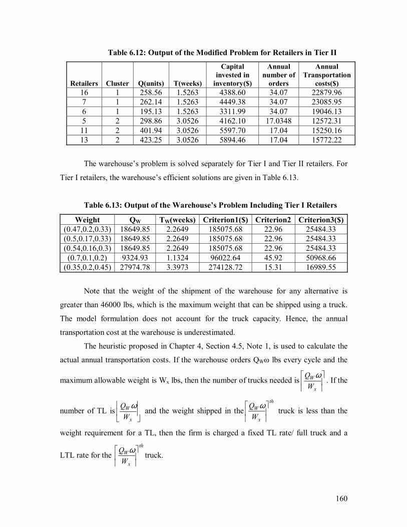
160
Table 6.12: Output of the Modified Problem for Retailers in Tier II
Retailers Cluster Q(units) T(weeks)
Capital invested in
inventory($)
Annual number of
orders
Annual Transportation
costs($) 16 1 258.56 1.5263 4388.60 34.07 22879.96 7 1 262.14 1.5263 4449.38 34.07 23085.95 6 1 195.13 1.5263 3311.99 34.07 19046.13 5 2 298.86 3.0526 4162.10 17.0348 12572.31 11 2 401.94 3.0526 5597.70 17.04 15250.16 13 2 423.25 3.0526 5894.46 17.04 15772.22
The warehouse�s problem is solved separately for Tier I and Tier II retailers. For
Tier I retailers, the warehouse�s efficient solutions are given in Table 6.13.
Table 6.13: Output of the Warehouse�s Problem Including Tier I Retailers
Weight QW TW(weeks) Criterion1($) Criterion2 Criterion3($)(0.47,0.2,0.33) 18649.85 2.2649 185075.68 22.96 25484.33 (0.5,0.17,0.33) 18649.85 2.2649 185075.68 22.96 25484.33 (0.54,0.16,0.3) 18649.85 2.2649 185075.68 22.96 25484.33 (0.7,0.1,0.2) 9324.93 1.1324 96022.64 45.92 50968.66
(0.35,0.2,0.45) 27974.78 3.3973 274128.72 15.31 16989.55
Note that the weight of the shipment of the warehouse for any alternative is
greater than 46000 lbs, which is the maximum weight that can be shipped using a truck.
The model formulation does not account for the truck capacity. Hence, the annual
transportation cost at the warehouse is underestimated.
The heuristic proposed in Chapter 4, Section 4.5, Note 1, is used to calculate the
actual annual transportation costs. If the warehouse orders QWω lbs every cycle and the
maximum allowable weight is Wx lbs, then the number of trucks needed is
x
W
WQ ω . If the
number of TL is
x
W
WQ ω and the weight shipped in the
th
x
W
WQ
ω truck is less than the
weight requirement for a TL, then the firm is charged a fixed TL rate/ full truck and a
LTL rate for the th
x
W
WQ
ω truck.
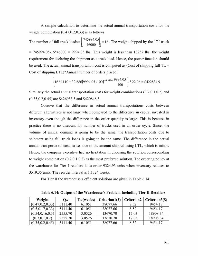
161
A sample calculation to determine the actual annual transportation costs for the
weight combination (0.47,0.2,0.33) is as follows:
The number of full truck loads 1646000
05.745994 =
= . The weight shipped by the 17th truck
= 745994.05-16*46000 = 9994.05 lbs. This weight is less than 18257 lbs, the weight
requirement for declaring the shipment as a truck load. Hence, the power function should
be used. The actual annual transportation cost is computed as (Cost of shipping full TL +
Cost of shipping LTL)*Annual number of orders placed:
( ) 9.422834$96.22*100
9994.05100 9994.05686.321110*16 3484.0 =
+ −
Similarly the actual annual transportation costs for weight combinations (0.7,0.1,0.2) and
(0.35,0.2,0.45) are $426953.5 and $420848.5.
Observe that the difference in actual annual transportations costs between
different alternatives is not large when compared to the difference in capital invested in
inventory even though the difference in the order quantity is large. This is because in
practice there is no discount for number of trucks used in an order cycle. Since, the
volume of annual demand is going to be the same, the transportation costs due to
shipment using full truck loads is going to be the same. The difference in the actual
annual transportation costs arises due to the amount shipped using LTL, which is minor.
Hence, the company executive had no hesitation in choosing the solution corresponding
to weight combination (0.7,0.1,0.2) as the most preferred solution. The ordering policy at
the warehouse for Tier I retailers is to order 9324.93 units when inventory reduces to
3519.35 units. The reorder interval is 1.1324 weeks.
For Tier II the warehouse�s efficient solutions are given in Table 6.14.
Table 6.14: Output of the Warehouse�s Problem Including Tier II Retailers
Weight QW TW(weeks) Criterion1($) Criterion2 Criterion3($)(0.47,0.2,0.33) 5111.40 6.1051 38077.66 8.52 9454.17 (0.5,0.17,0.33) 5111.40 6.1051 38077.66 8.52 9454.17 (0.54,0.16,0.3) 2555.70 3.0526 13670.70 17.03 18908.34 (0.7,0.1,0.2) 2555.70 3.0526 13670.70 17.03 18908.34
(0.35,0.2,0.45) 5111.40 6.1051 38077.66 8.52 9454.17
162
Again, the actual annual transportation costs must be computed. The actual annual
transportation costs for QW = 5111.40 units and QW = 2555.70 units are $47271.70 and
$49174.85. In the former, all the shipments are using TL while in the latter, two full TL
and one LTL is used. Since the difference in actual annual transportation is less when
compared to the difference in capital invested inventory, the company executive decided
to go with the alternative that has the least inventory capital which is either weight
combination (0.54,0.16,0.3) or (0.7,0.1,0.2). The ordering policy for the warehouse to
serve its Tier II retailers is to order 2555.70 units when inventory reduces to 357.83 units.
The reorder interval is 3.0526 weeks.
To use the value path method, the ideal value of the criteria must be determined.
The ideal value is obtained by optimizing the criterion independent of another. Since we
use a heuristic to determine the actual annual transportation costs, the value path method
cannot be used.
The executive of the Fortune 500 company who was the DM for the warehouse,
preferred the multi-criteria methodology over the single objective methodology for
determining ordering policies. He felt more involved in the decision making process as
he had to evaluate tradeoffs and use his judgment to choose the most preferred solution.
This further validated the advantages of using a multi-criteria approach. Also, the
cognitive burden during the decision making process was less as he had to analyze the
tradeoff information among three efficient solutions.
6.5 Case Study 3: Chapter 5
6.5.1 Overview
In this study, the models and methodology developed in Chapter 5 are applied to
solve the inventory planning problem when there is uncertainty in the system in the form
of stochastic demands and stochastic lead times. In addition to the three criteria in the
previous study, fill rate (FR) is the fourth criterion and is used to measure customer
satisfaction. Since the locations are assumed to follow a continuous review policy, the
reorder interval is a random variable. The decision variables are order quantity and
reorder point. Due to high FR maintained by the company, the average time spent by the
system in a stockout situation is small. In general, this is also true for the retailers. Excess

163
demand is treated as lost sales at all the locations. As in Case Study 2, retailers�
shipments are LTL and the warehouse�s shipment is TL. The DM for each location must
specify upper and lower bounds on the order quantity and the reorder point. Since we
were using monthly data, the demands were large enough to approximate either the
Poisson or geometric Poisson distribution by a normal distribution. Hence, it was
sufficient to check for the normality of the monthly demand data. The K-S test
(Ravindran et al., 1987, pp. 622-623) in Minitab was used to check for normality. The
results are given in Table 6.15.
Table 6.15: Normality Test for Demand
Retailers K-S test Mean Standard deviation 1 ! 1603 710.6 2 ! 1445 830 3 ! 1944 1170 4 ! 4424 1118 5 ! 477.3 166.8 6 ! 623.3 364.2 7 ? 1083 1463 8 ! 3190 1235 9 ! 6068 823.3
10 ! 3583 899.6 11 ! 641.9 425.2 12 ! 3867 1564 13 ! 675.9 272.7 14 X 2794 1375 15 ! 2347 586 16 ! 825.9 416.8 17 ! 1338 360 18 ! 4836 833.8 19 X 921.7 336 20 ! 1781 415.5
Assuming a significance level of 0.05, the demand for most of the retailers can be
approximately described by a normal distribution. For Retailers 14 and 19, the p values
are 0.043 and 0.046, respectively. For Retailer 7, the test is inconclusive as the p value is
less than 0.01. We believe that approximating the demand for these retailers as a normal
distribution would not cause any serious deviation in the ordering policy.
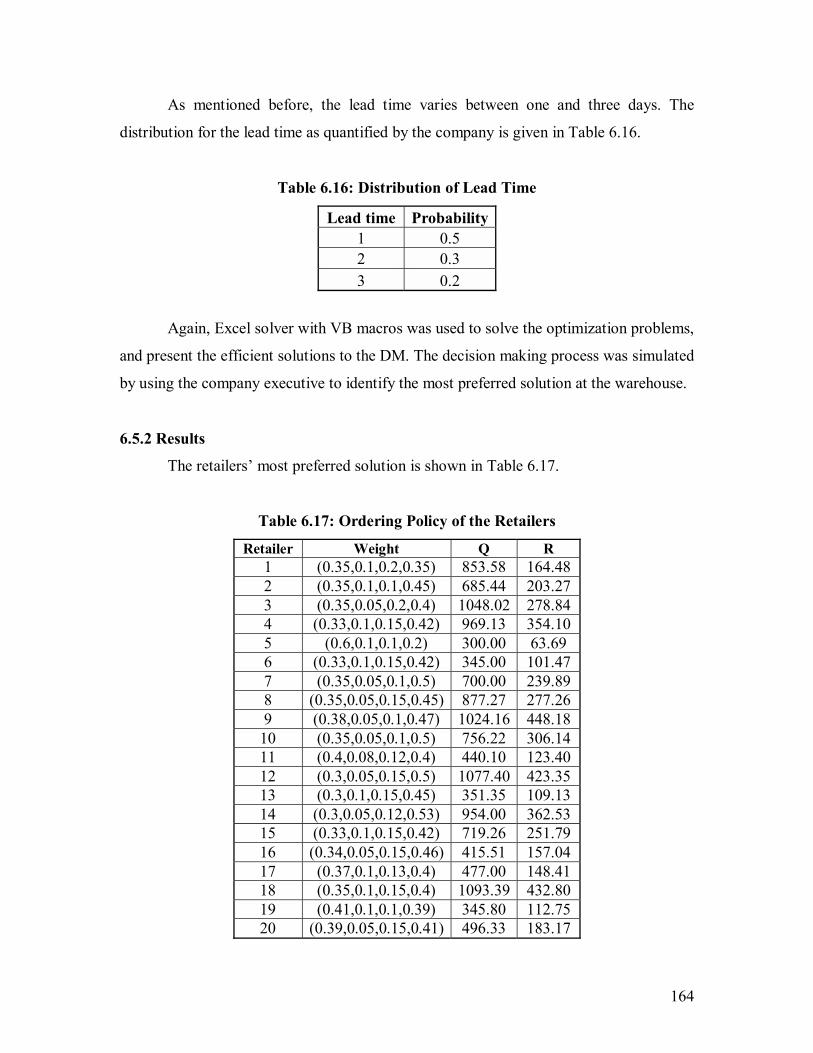
164
As mentioned before, the lead time varies between one and three days. The
distribution for the lead time as quantified by the company is given in Table 6.16.
Table 6.16: Distribution of Lead Time
Lead time Probability1 0.5 2 0.3 3 0.2
Again, Excel solver with VB macros was used to solve the optimization problems,
and present the efficient solutions to the DM. The decision making process was simulated
by using the company executive to identify the most preferred solution at the warehouse.
6.5.2 Results
The retailers� most preferred solution is shown in Table 6.17.
Table 6.17: Ordering Policy of the Retailers
Retailer Weight Q R 1 (0.35,0.1,0.2,0.35) 853.58 164.48 2 (0.35,0.1,0.1,0.45) 685.44 203.27 3 (0.35,0.05,0.2,0.4) 1048.02 278.84 4 (0.33,0.1,0.15,0.42) 969.13 354.10 5 (0.6,0.1,0.1,0.2) 300.00 63.69 6 (0.33,0.1,0.15,0.42) 345.00 101.47 7 (0.35,0.05,0.1,0.5) 700.00 239.89 8 (0.35,0.05,0.15,0.45) 877.27 277.26 9 (0.38,0.05,0.1,0.47) 1024.16 448.18
10 (0.35,0.05,0.1,0.5) 756.22 306.14 11 (0.4,0.08,0.12,0.4) 440.10 123.40 12 (0.3,0.05,0.15,0.5) 1077.40 423.35 13 (0.3,0.1,0.15,0.45) 351.35 109.13 14 (0.3,0.05,0.12,0.53) 954.00 362.53 15 (0.33,0.1,0.15,0.42) 719.26 251.79 16 (0.34,0.05,0.15,0.46) 415.51 157.04 17 (0.37,0.1,0.13,0.4) 477.00 148.41 18 (0.35,0.1,0.15,0.4) 1093.39 432.80 19 (0.41,0.1,0.1,0.39) 345.80 112.75 20 (0.39,0.05,0.15,0.41) 496.33 183.17
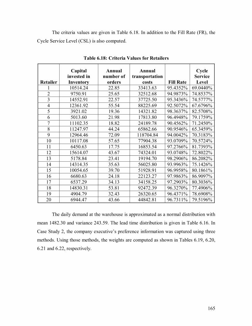
165
The criteria values are given in Table 6.18. In addition to the Fill Rate (FR), the
Cycle Service Level (CSL) is also computed.
Table 6.18: Criteria Values for Retailers
Retailer
Capital invested in Inventory
Annual number of
orders
Annual transportation
costs Fill Rate
Cycle Service Level
1 10514.24 22.85 33413.63 95.4352% 69.0440%2 9750.91 25.65 32512.68 94.9873% 74.8537%3 14552.91 22.57 37725.50 95.3436% 74.5777%4 12361.92 55.54 88225.69 92.5072% 67.6796%5 3921.02 19.36 14321.82 98.3637% 82.5708%6 5013.60 21.98 17813.80 96.4948% 79.1759%7 11102.35 18.82 24189.78 90.4562% 71.2450%8 11247.97 44.24 65862.66 90.9546% 65.3459%9 12964.46 72.09 118704.84 94.0042% 70.3183%10 10117.08 57.65 77904.38 93.0709% 70.5724%11 6450.63 17.75 16853.54 97.2766% 81.7393%12 15614.07 43.67 74324.01 93.0748% 72.8022%13 5178.84 23.41 19194.70 98.2906% 86.2082%14 14314.35 35.63 56025.80 93.9963% 75.1426%15 10054.65 39.70 51928.91 96.9958% 80.1861%16 6680.63 24.18 22123.27 97.9863% 86.9097%17 6537.29 34.13 34158.25 97.2903% 80.3036%18 14830.31 53.81 92472.39 96.3270% 77.4906%19 4904.79 32.43 26320.65 96.4371% 78.6908%20 6944.47 43.66 44842.81 96.7311% 79.5196%
The daily demand at the warehouse is approximated as a normal distribution with
mean 1482.30 and variance 243.59. The lead time distribution is given in Table 6.16. In
Case Study 2, the company executive�s preference information was captured using three
methods. Using those methods, the weights are computed as shown in Tables 6.19, 6.20,
6.21 and 6.22, respectively.

166
Table 6.19: Weights Using Method 1
Criteria Score (1-10) Weights Capital invested in inventory 7 7/25=0.28
Annual number of orders 3 3/25=0.12 Annual transportation costs 5 5/25=0.2
Fill rate 10 10/25=0.4 Total 25
Table 6.20: Weights Using Method 2
Criterion 1 Criterion 2 Criterion 3 Criterion 4 Total Weights Criterion 1 1 1 1 0 3 3/10=0.3Criterion 2 0 1 0 0 1 1/10=0.1Criterion 3 0 1 1 0 2 2/10=0.2Criterion 4 1 1 1 1 4 4/10=0.4 10
Table 6.21: Method 3-Strength of Preferences
Criterion 1 Criterion 2 Criterion 3 Criterion 4 Criterion 1 1 3 2 1/2 Criterion 2 1/3 1 ½ 1/4 Criterion 3 1/2 2 1 1/3 Criterion 4 2 4 3 1 Column sum 3.83 10 6.5 2.08
Table 6.22: Weights Using Method 3
Criterion 1 Criterion 2 Criterion 3 Criterion 4 Weights Criterion 1 0.26 0.33 0.31 0.24 0.285 Criterion 2 0.09 0.1 0.08 0.12 0.09 Criterion 3 0.13 0.2 0.15 0.16 0.16 Criterion 4 0.52 0.4 0.46 0.48 0.465
The weight combinations that best describe the company executive�s preference
are (0.28,0.12,0.2,0.4), (0.3,0.1,0.2,0.4), and (0.285,0.09,0.16,0.465). The efficient
solutions for the warehouse are given in Table 6.23.

167
Table 6.23: Efficient Solutions for Warehouse
Weights Q R Criterion1 Criterion2 Criterion3 Criterion4(0.28,0.12,0.2,0.4) 23810.12 4479.67 265000.92 22.72 25222.18 99.9888% (0.3,0.1,0.2,0.4) 22273.24 4479.54 250321.44 24.29 26962.54 99.9880%
(0.285,0.09,0.16,0.465) 20862.19 4493.45 237096.99 25.93 28786.19 99.9908%
The CSL values are 93.7683%, 93.7548% and 95.1488%, respectively. After
observing the criteria values in Table 6.23, the company executive felt that the capital
invested in inventory was on the higher side. By increasing the weight assigned to the
capital invested in inventory and decreasing the weight assigned to FR, a new efficient
solution was obtained. The new weight combination was (0.42,0.09,0.16,0.33). The
criteria values corresponding to this combination were: Capital invested in inventory =
$201573.31, Annual number of orders = 31.46, Annual transportation costs = $34918.55
and Fill rate = 99.9778 %. The CSL was computed to be 91.9735%. The ordering policy
of the warehouse was to order 17198.39 units when the reorder point reached 4463.57
units.
As in Case Study 2, the weight of the warehouse�s shipment was greater than
46000 lbs, the weight of a single truck. Hence, the annual transportation cost was
underestimated. By using the same heuristic method in Section 6.4.3, the actual annual
transportation cost was calculated as $573993.71. The warehouse would use 15 trucks to
transport this shipment.
6.6 Summary
In this chapter we showed that the theoretical models developed in this thesis can
be used for inventory planning for a product produced by a Fortune 500 consumer
products company under different scenarios. We had to make suitable modifications to
the existing methodologies to account for some problems faced while adapting them to
the real world data. This study further validated some of the advantages of using a multi-
criteria methodology for determining inventory policies in a decentralized supply chain.
Chapter 7 discusses the conclusions of this research and future work.

168
Chapter 7
CONCLUSIONS AND FUTURE WORK
7.1 Overview
The highly competitive nature of today�s market makes it extremely difficult for a
company to function as an independent entity. A company is better off being part of a
supply chain where they can contribute to the profitability of the supply chain by
concentrating on its core competencies. Thus, each company will have its own Decision
maker (DM) trying to optimize its own objectives. To be successful, the company has to
integrate and coordinate its activities with the activities of the rest of the supply chain.
This is one of the major challenges facing supply chains today, and what is termed as
�seamless� integration has still not been achieved. Achieving integration and
coordination is dependent on the ability of the companies within the supply chain to share
real time data. This is in turn dependent on the willingness of the companies to
collaborate with each other and the IT capabilities that are in place.
Inventory management is a vital function that companies within supply chains
must continually focus on as it leads to enormous cost savings not only for the individual
companies but also for the entire supply chain. Each company must plan its inventory
carefully so as to not stock too much and at the same time meet the demands of the
downstream companies. There is a cascading effect in the sense that the inability to meet
the demands of the downstream companies will translate into the end consumers not
getting what they want. In the current environment where consumers are not willing to
wait, they will turn to a competitor�s products. Hence, it is important to have the right
inventory, in the right quantities, at the right place, at the right time.
Other functions such as transportation, facilities location, routing, etc. influence
inventory ordering policies. Hence, it is important to consider one or more of these
functions while determining the inventory policy at each location. As explained in
Chapter 1, transportation costs contribute more to the GDP of the United States than
inventory costs. Also, transportation costs are expected to rise in the future. Hence, it is
of paramount importance to integrate the transportation function while determining
inventory policies.

169
There are often several criteria of interest other than cost that conflict with each
other. It is usually difficult to estimate a cost associated with these criteria in practice.
One of the main advantages of using multi-criteria optimization techniques is that it can
model conflicting criteria without using the cost information that is essential in solving
single objective optimization models.
Inter-functional decisions are made by evaluating the tradeoffs associated with
different alternatives. A multi-criteria approach offers the DM exactly this, wherein, by
assigning different weights to each criterion, several efficient solutions (alternatives) can
be generated from which the most preferred solution is chosen. In this way the DM
incorporates his/her preference information in the final ordering policy. A single
objective optimization model provides the DM with a single optimal or heuristic solution,
which is independent of the DM�s preference information.
7.2 Conclusions
Keeping the importance of coordination in supply chains we first proposed a
modified base period policy using a single objective framework when demands are
assumed to be deterministic. The objective of the policy was to enable the warehouse to
have a better visibility of all the retailer orders so that it can plan its inventory and at the
same time meet the demands of the retailers without deviating too much from their
requirements. Instead of specifying an arbitrary value for the base period (as is common
in the literature), a performance metric that measures how quickly a retailer turns over its
inventory is used. This was validated by a Fortune 500 consumer products company.
Using this metric and the structure of the optimal solution, the warehouse can evaluate its
retailers, and classify them into clusters based on how important they are to the
warehouse. This policy was tested with real world data obtained from a Fortune 500
company for one of its functional products which is non-seasonal and non-perishable.
Based on the results, it was concluded that the policy performed very well for the retailers
for a wide range of demand data, i.e., the warehouse was able to meet the requirements
without deviating too much from the optimal policy. However, the range of the demand
data had an impact on the ordering period of the warehouse in the sense that to
accommodate all the retailers, the warehouse had to order in larger quantities increasing

170
its inventory holding costs. One way of circumventing this problem was for the
warehouse to group the clusters of retailers into Tier I, Tier II, etc. and re-solve the
problem independently for each tier.
To avoid the problem of estimating marginal cost information and to incorporate
the DM�s preference information, we formulated the above problem as a multi-criteria
problem where transportation costs were considered between the echelons. The three
criteria that were considered were the capital invested in inventory, annual number of
orders placed and, annual transportation costs. Transportation costs were modeled using
continuous functions that best fit the freight rate data. Under the assumption that the
retailers� shipments were LTL and the warehouse�s shipment was TL, efficient solutions
were derived. The value path method was used to graphically display the tradeoff
information to the DM. A general model was formulated which will indicate to each
location whether to use TL or LTL depending on the weigh of the shipment. The former
model (where retailers� shipments are LTL and warehouse�s shipment is TL) was tested
with the same data set used in the previous chapter. To make the decision making process
more realistic, an executive from the Fortune 500 company was asked to be the DM. His
preference information was obtained using standard multi-criteria techniques such as
rating method, pairwise comparison method and AHP. The weights obtained from the
different methods were used to generate a set of efficient solutions. Based on the
feedback we received, the company executive was very comfortable with the multi-
criteria model since he had the option of choosing from several different efficient
solutions. He was able to analyze the tradeoffs in an easy manner. By assigning more
priority to a particular criterion he was able to obtain the solution of his preference. One
of the problems faced while using the theoretical model was due to the range of the
retailer demand data. The other problem was due to the assumption that the truck
employed by the warehouse did not have any capacity constraint. Hence, the
transportation cost at the warehouse was underestimated. We provided a simple heuristic
to resolve this issue.
In the last part of the thesis, we modeled and solved the multi-criteria inventory
problem with transportation costs when both demand and lead times were assumed to be
random variables. Fill rate (FR) was used as the fourth criterion to measure customer
171
service. From a modeling standpoint it is important to determine the distribution of the
lead time demand (LTD). For the case of Poisson and normal demands and lead times
following any discrete distribution, we used the convex combination approach to quantify
the LTD as Poisson and normal respectively. We proved that the convex combination
approach can also be used for the case of a geometric Poisson demand. Using renewal
theory concepts and the convex combination approach, the LTD at the warehouse was
characterized as a normal distribution. Efficient solutions were generated by changing the
weights assigned to the criteria. We recommend the use of a cycle service level (CSL) in
conjunction with the FR criterion, since there is a possibility that CSL could be very low
even when the FR is at an acceptable level. Value path graphs were used to present the
tradeoffs to the DM. The model was tested with same data set. Again, we used a real DM
to determine the ordering policy at the warehouse by evaluating the tradeoffs associated
with the four criteria.
Microsoft Excel was used to implement the models developed in this thesis. For
the single objective model, Excel was used with VB macros to automate the solution
methodology and generate optimal solutions. For the models developed in Chapter 4 and
Chapter 5, Excel Solver was used with VB macros to solve for different efficient
solutions according to the weight inputs provided by the DM.
7.3 Managerial Implications
A summary of some of the important managerial implications of the models
developed in this thesis are as follows:
• The cluster analysis developed using model 1 can be used by a company with
other performance metrics to identify their best customers. This is important due
to the concept of revenue management gaining momentum in supply chains.
Based on this cluster analysis, the company can provide better service to its most
preferred customers.
• The models developed in the thesis can be used by a company to serve its
customers that face non-identical demands. For example, for models 1 and 2, we
use a tier based approach to reduce costs at the company, and at the same time
maintain the quality of the solution at the customers. For the stochastic case in
172
model 3, we construct the demand process at the warehouse under the assumption
that the external demands are non-identical random variables.
• Models 2 and 3 (the multi-criteria models) were specifically developed to involve
the manager (DM) of a company in the solution process so that the ordering
policy reflects the manager�s preference information. The preference information
in the form of weights of the criteria is obtained by using standard methods
discussed in Chapter 6. These weights are used in the optimization problem to
generate the efficient solutions. To enable the manager choose the most preferred
solution, a graphical based tool called value path method is used to present the
tradeoff information. Tradeoff analysis can be performed by changing the weights
assigned to the criteria. Since the manager analyzes the tradeoff information, the
chosen solution reflects his/her�s preference.
• What-if analysis can be performed by changing the parameters such as the
number of retailers, demand and lead time distributions, cost of the product, etc.
7.4 Limitations
Some of the limitations of the models developed in this thesis are:
• The models are restricted to two echelons/stages.
• The manufacturer that supplies the warehouse is assumed to have infinite
capacity.
• The demands faced by the retailers are assumed to be stationary, or demand
distributions that do not vary with time.
7.5 Future Work
This section describes some possible extensions from this thesis and in general
other emerging areas in the field of supply chain management.
• This work can be extended by incorporating the facilities location function and
analyze how transportation costs and inventory policies are affected. Treating the
problem from a multi-criteria perspective will facilitate capturing all the necessary
tradeoff information before choosing the final solution.

173
• An interesting problem that is still in its nascent stage is quantifying risks in
supply chains. This is relevant due to global outsourcing. Outsourcing is done
primarily to take advantage of cheap labor and raw materials. However,
companies fail to take into account the risk factor, e.g., stability of suppliers,
disruptions in the flow of goods due to uncontrollable events, long lead times, etc.
Incorporating these factors in an integrated framework is essential for the supply
chain to first decide if the outsourcing venture is going to be beneficial. It then has
to decide how it can continue to provide the same level of service as there is an
increase in transit time. Again, it would be advantageous to treat it as a multi-
criteria problem due to the number of conflicting criteria and to quantify the
tradeoffs associated with these criteria.
• For coordination schemes such as the one proposed in Chapter 3 to work
successfully, the benefits (profits) obtained as a result of following the scheme
must be shared fairly among the various partners in the supply chain. This will
enable these companies to collaborate on a more frequent basis, which is a
cornerstone for resolving conflicts and improving existing partnerships.

174
BIBLIOGRAPHY
1. Abdul-Jalbar, B., Gutiererez, J., Puerto, J., Sicilia, J. (2003), �Policies for
inventory/distribution systems: The effect of centralization vs. decentralization�,
International Journal of Production Economics, 81-82, 281-293.
2. Adelson, R.M. (1966), �Compound Poisson distributions�, Operational Research
Quarterly, 17(1), 73-75.
3. Agrell, P.J. (1995), �A multi-criteria framework for inventory control�,
International Journal of Production Economics, 41, 59-70.
4. Andersson, J., Melchirors, P. (2001), �A two-echelon inventory model with lost
sales�, International Journal of Production Economics, 69, 307-315.
5. Archibald, B.C. (1981), �Continuous review (S, s) policies with lost sales�,
Management Science, 27(10), 1171-1177
6. Arthur, J.L, Ravindran, A. (1980), �An efficient goal programming algorithm for
linear goal programming problems�, ACM Transactions on Mathematical
Software, 6(3), 378-386.
7. Arthur, J.L, Ravindran, A.(1980), �A Branch and Bound algorithm with constraint
partitioning for solving integer goal programming problems �, European Journal
of Operational Research, 4(6), 421-425.
8. Axsater, S. (1990), �Simple solution procedures for a class of two-Echelon
inventory problems�, Operations Research, 38, 64-69.
9. Axsater, S. (1993), �Exact and approximate evaluation of batch ordering policies
for two level inventory systems�, Operations Research, 41(4), 777-785.
10. Axsäter, S., Rosling, K. (1993), �Notes: Installation vs. Echelon stock policies for
Multilevel Inventory Control�, Management Science, 39(10), 1274-1280.
11. Axsäter, S., Juntti, L. (1996), �Comparison of Echelon stock and Installation
stock policies for two-level inventory systems�, International Journal of
Production Economics, 45, 303-310.
12. Ballou, R.H. (1991), �The accuracy in estimating truck class rates for logistical
planning�, Transportation Research: Part A, 25A (6), 327-337.

175
13. Ballou, R.H., �Business Logistics/Supply Chain Management� 5th Edition
Prentice-Hall, New Jersey (2003).
14. Baumol, W.J, Vinod, H.D. (1970), �An inventory-theoretic model of freight
transport demand�, Management Science, 16(7), 413-421.
15. Bookbinder, J.H, Chen, V.Y.X (1992), �Multi-criteria tradeoffs in a
warehouse/retailer system�, Journal of the Operational Research Society, 43(7),
707-720.
16. Brown, R.G., �Decision Rules for Inventory Management� Holt, Rinehart and
Winston, New York (1961).
17. Buffa, F.P., Reynolds, J.I. (1977), �The inventory-transport model with sensitivity
analysis by indifference curves�, Transportation Journal, 2(16), 83-90
18. Carter, J.R., Ferrin, B.G, (1996), �Transportation costs and inventory
management: Why transportation costs matter�, Production and Inventory
Management Journal, 37(3), 58-61.
19. Chan, L.M.A, Muriel, A., Shen, Z.M., Simchi-Levi, D., Teo, C. (2002), �Effective
zero-inventory-ordering policies for the single warehouse multi-retailer problem
with piecewise linear cost structures�, Management Science, 48(11), 1446-1460.
20. Chopra, S., Meindl, P., �Supply Chain Management � Strategy Planning and
Operation� Prentice Hall, New Jersey (2001).
21. Constable, G.K., Whybark, D.C. (1978), �The interaction of transportation and
inventory decisions�, Decision Sciences, 9(4), 688-699.
22. Cook, A.J. (2006), �Logistics cost under pressure�, Logistics Management.
http:\\www.logisticsmgmt.com/article/CA6352889.html, access date: 09/15/2006.
23. Crowston, W.B., Wagner, M., Williams, J.F. (1973), �Economic lot size
determination in multi-stage assembly systems�, Management Science, 19(5),
517-527.
24. Das, C. (1974), � Choice of transport service: An inventory theoretic approach�,
The Logistics and Transportation Review, 10(2), 181-187.
25. DeBodt, M.A, Graves, S.C. (1985), �Continuous review policies for a multi-
echelon inventory problem with stochastic demand�, Management Science, 31,
1286-1295.

176
26. Deuermeyer, B., Schwarz, L.B, �A model for the analysis of system service level
in warehouse/retailer distribution systems: The identical retailer case�, Studies in
Management Science, 16, North-Holland publishing company, 163-193 (1981).
27. DiFillipo, T., �Multi-criteria supply chain inventory models with transportation
costs�, Masters Thesis, Department of Industrial Engineering, Pennsylvania State
University (2003).
28. Eppen, G.D., Martin, R.K. (1988), �Determining Safety Stock in the presence of
stochastic lead time and demand�, Management Science, 34(11), 1380-1390.
29. Feeney, G.J., Sherbrooke, C.C. (1966), �The (S-1, S) Inventory policy under
Compound Poisson demand�, Management Science, 12(5), 391-411.
30. Feller, W., �An Introduction to Probability theory and Applications�, Vol.1, John
Wiley and Sons, New York (1957).
31. Forsberg, R. (1996), �Exact evaluation of (R,Q) policies for two level inventory
systems with Poisson demand�, European Journal of Operational Research, 96,
130-138.
32. Ganeshan, R, �Analytical Essays in Supply chain management�, PhD Thesis,
Department of Management Science and Information Systems, Pennsylvania
State University (1997).
33. Ganeshan, R. (1999), �Managing supply chain inventories: A multiple retailer,
one warehouse, multiple supplier model�, International Journal of Production
Economics, 59, 341-354.
34. Gardner, E.S., Dannenbring, D.G (1979), �Using optimal policy surfaces to
analyze aggregate inventory tradeoffs�, Management Science, 25(8), 709-720.
35. Geoffrion, A.M. (1968), �Proper efficiency and theory of vector maximization�,
Journal of Mathematical Analysis and Applications, 22, 618-630.
36. Geunes, J., Zeng, A.Z. (2003), �Optimizing supply shortage decisions in base
stock distributions operations�, Journal of Global Optimization, 26, 25-42.
37. Graves, S.C. (1985), �A multi-Echelon inventory model for a repairable item with
one-for-one replenishment�, Management Science, 31, 1247-1256.
38. Hadley, G., Whitin, T.M,. �Analysis of Inventory systems� Prentice Hall,
Englewood Cliffs, New Jersey (1963).

177
39. Ignizio, J.P, �Goal Programming and Extensions�, D.C. Heath, Lexington, MA
(1976).
40. Johansen, S.G., Thorstenson, A. (2004), �The (r,q) policy for the lost-sales
inventory system when more than one order may be outstanding�, Working Paper
L-2004-03, Logistics/SCM Research Group, School of Business, University of
Aarhus.
41. Langley, C.J (1980), �The inclusion of transportation costs in inventory models:
Some considerations�, Journal of Business Logistics, 2(1), 106-125.
42. Lee, C. (1986), �The economic order quantity for freight discount costs�, IIE
Transactions, 8, 318-320.
43. Lee, S.M., �Goal Programming for Decision Analysis�, Auerbach, Philadelphia,
PA (1972).
44. Lee, H., Whang, S. (1999), �Decentralized multi-echelon supply chains:
incentives and information�, Management Science, 45(5), 633-640.
45. Love, S.F. (1972), �A facilities in Series Inventory model with nested schedules�,
Management Science, 18(5), 327-338.
46. Magretta, J. (1998), �The power of virtual integration: An interview with Dell
Computer�s Michael Dell�, Harvard Business Review, 76(2), 73-84.
47. Mason, S.J, Magableh, G.M, Ramasami, B., Kutanoglu, E. (2004), �Integrated
analysis of transportation and inventory in inter-modal distribution networks�,
Final report for MBTC project 2041,
http://www.mackblackwell.org/OLD/research/finals/arc2041/MBTC%202041%2
0Final%20Report.pdf, access date: 11/21/2004.
48. Min, H., Zhou, G. (2002), �Supply chain modeling- Past, present and future�,
Computers and Industrial Engineering, 43, 231-249.
49. Nahmias, S. (1979), �Simple approximations for a variety of dynamic lead time
lost sales inventory models�, Operations Research, 27(5)
50. Nahmias, S., Smith, S.A. (1994), �Optimizing Inventory levels in a two-echelon
retailer system with partial lost sales�, Management Science, 40(5), 582-596
51. Nahmias, S., �Production and Operations Analysis� McGraw-Hill, New York
(2001).
178
52. Nozick, L.K, Turnquist, M.A (2001), �Inventory, transportation, service quality
and the location of distribution centers: Case study�, European Journal of
Operational research, 129, 362-371.
53. Perl, J., Sirisoponsilp, S. (1988) �Distribution networks: Facility location,
transportation and inventory�, International Journal of Physical Distribution and
Materials Management, 13(1), 18-26.
54. Qu, W.W, Bookbinder, J.H, Iyogun, P. (1999), �An integrated inventory-
transportation systems with modified periodic policy for multiple products�,
European Journal of Operational Research, 115, 254-269.
55. Rangarajan, A., Ravindran, A. (2005), �A base period inventory policy for
decentralized supply chains�, Working Paper 05-04, Center for Supply Chain
Research, Smeal College of Business, Penn State University.
56. Ravindran, A., Phillips, D., Solberg, J., �Operations Research-Principles and
Practice� Wiley, New York (1987).
57. Ravindran, A. (2002), �Lecture notes from course IE-570, Supply Chain
Engineering�, Department of Industrial Engineering, Penn State University.
58. Ravindran, A. (2003), �Lecture notes from course IE-520, Multi-Criteria
Optimization�, Department of Industrial Engineering, Penn State University.
59. Ross, S.M., �Introduction to Probability Models, 7th Edition� Academic Press,
San Diego, CA (2000).
60. Roundy, R. (1985), �98%-effective integer ratio lot sizing for one-warehouse
multi-retailer systems�, Management Science, 31(11), 1416-1430.
61. Saaty, T.L., �The Analytical Hierarchy Process� McGraw-Hill, New York
(1980).
62. Schilling, D.A., Revelle, C., Cohon, J. (1983), �An approach to the display and
analysis of multi-objective problems�, Socio-Economic Planning Sciences, 17 (2),
57-63
63. Schwarz, L.B. (1973), �A simple continuous review deterministic one-warehouse
N-retailer inventory problem�, Management Science, 19(5), 555-566.
179
64. Schwarz, L.B, Ward, .J, Zhai, X. (2004), �Joint transportation and inventory
problems in supply chains: A review, Working paper, Krannert School of
Management, Purdue University.
65. Sherbrooke, C.C. (1968a), �Discrete compound Poisson processes and tables of
the Geometric Poisson distribution�, Naval Research Logistics Quarterly, 15,
189-203.
66. Sherbrooke, C.C. (1968b), �METRIC: A multi-Echelon technique for
recoverable item control�, Operations Research, 19, 761-777.
67. Shin, W.S, Ravindran, A (1991), �Interactive multiple objective optimization
survey I � Continuous case�, Computers and Operations Research, 18(1), 97-114.
68. Silver, E.A., Peterson, R., �Decision Systems for Inventory Management and
Production Planning�, John Wiley and Sons, New York (1985).
69. Smith, S.A. (1977), �Optimal inventories for an (S-1, S) system with no
backorders�, Management Science, 23(5), 522-531.
70. Starr, M.K., Miller, D.W, �Inventory control: Theory and Practice� Prentice Hall,
New Jersey, Englewood Cliffs (1963).
71. Steuer, R.E (1976), �Multiple objective linear programming with interval criterion
weights�, Management Science, 23(3), 305-317.
72. Steuer, R.E, �Multiple Criteria Optimization: Theory, Computation, and
Application� John Wiley and Sons, New York (1986).
73. Svoronos, A., Zipkin, P. (1988), �Estimating the performance of multi-level
inventory systems�, Operations Research, 36(1), 57-72.
74. Swenseth, S.R, Godfrey, M.R (1996), �Estimating freight rates for logistics
decisions�, Journal of Business Logistics, 17(1), 213-231.
75. Swenseth, S.R, Godfrey, M.R (2002), �Incorporating transportation costs into
inventory replenishment decisions�, International Journal of Production
Economics, 77, 113-130.
76. Toptal, A., Cetinkaya, A., Lee, C. (2003), �The buyer-vendor coordination
problem: Modeling inbound and outbound cargo capacity and costs�, IIE
Transactions, 35, 987-1002.

180
77. Thirumalai, R., �Multi-criteria-Multi decision maker inventory models for serial
supply chains�, PhD Thesis, Department of Industrial Engineeering, Pennsylvania
State University (2001).
78. Tyworth, J.E. (1991), �The inventory-theoretic approach in transportation
selection models: A critical review�, Logistics and Transportation Review, 27(4),
299-318.
79. Tyworth, J.E. (1992), �Modeling transportation-inventory tradeoffs in a stochastic
setting�, Journal of Business Logistics, 13(2), 97-124.
80. Tyworth, J.E., Zeng, A. (1998), �Estimating the effects of carrier transit-time
performance on logistics cost and service�, Transportation Research-A, 32(2), 89-
97.
81. Wagner, H.M., Whitin, T.M. (1958), �Dynamic version of the economic lot size
model�, Management Science, 5, 89-96.
82. Warsing, P.D., �Supply Chain Management�, To be published in Operations
Research and Management Science Handbook, CRC press, A.Ravindran (ed.),
(2007).
83. Walton, S.R. (2005), �Wal-Mart, Supplier-Partners, and the Buyer-Power Issue�,
Antitrust Law Journal, 72, 509-527.
84. Zeleny, M., �Multi-criteria Decision Making� McGraw-Hill, New York (1982).

VITA
Ajay Natarajan
EDUCATION PhD - Industrial Engineering and Operations Research, The Pennsylvania State University, University Park, PA, May 2007 M.S. - Industrial Engineering, The University of Texas at Arlington, Arlington, TX, May 2002, GPA - 3.67 B.E. � Mechanical Engineering, Madras University, India, May 2000, GPA � 3.45 INDUSTRIAL EXPERIENCE G.E., John. F. Welch Technology center, India, Intern, Information Decision Technology Lab, May2004-Aug 2004 �Worked on Collaborative Demand Management for Structured Products, a division of GE Advanced Materials. �Developed a Position Tracker prototype using Excel and VB macros. �Researched articles on managing uncertainty in Supply Chains. ADDITIONAL RELATED EXPERIENCE The Pennsylvania State University, Graduate Assistant, Jun 2005- Dec 2005 �Developed Case Studies for the course Engineering Economics. Teaching Assistant, Aug 2002-May 2005 �Courses include: Supply Chain Engineering, Linear Programming, Multiple Criteria Optimization, Engineering Statistics, Engineering Economics, Simulation and CAD/CAM. COMPUTING SKILLS Optimization packages: Excel Solver, Lindo, Lingo Simulation packages: Witness, Arena. Statistical Packages: Minitab, SAS Database: MS Access. Spreadsheet: MS Excel Design Package: Pro E ACHIEVEMENTS AND MEMBERSHIPS �Best outgoing intern award from GE, John.F.Welch Technology center in India (Summer 2004). �Tuition Grant-in-Aid award from the Graduate School, The Pennsylvania State University (Spring 2006). �Scholarship from the Department of Industrial and Manufacturing Systems Engineering, The University of Texas at Arlington (Spring and Summer 2001). �Vice-President, Industrial Engineering Graduate Association. �Member, Alpha Pi Mu. �Student Member of Institute for Operations Research and Management Sciences (INFORMS) affiliated to the Operations management society. �Student Member of Institute of Industrial Engineers (IIE).